NBER WORKING PAPER SERIES

THE GROWTH OF OBESITY AND TECHNOLOGICAL CHANGE:

A THEORETICAL AND EMPIRICAL EXAMINATION

Darius Lakdawalla

Tomas Philipson

Working Paper 8946

http://www.nber.org/papers/w8946

NATIONAL BUREAU OF ECONOMIC RESEARCH

1050 Massachusetts Avenue

Cambridge, MA 02138

May 2002

We wish to thank seminar participants at AEI, The University of Chicago, Columbia University, Harvard

University, MIT, The University of Toronto, UCLA, Yale University, the 2001 American Economic

Association Meetings, the 2001 Population Association of America Meetings, the 12 th Annual Health

Economics Conference, as well as Gary Becker, Shankha Chakraborty, Mark Duggan, Michael Grossman,

John Mullahy, Casey Mulligan, and Richard Posner. Neeraj Sood and Erin Krupka provided excellent

research assistance. The views expressed herein are those of the authors and not necessarily those of the

National Bureau of Economic Research.

© 2002 by Darius Lakdawalla and Tomas Philipson. All rights reserved. Short sections of text, not to

exceed two paragraphs, may be quoted without explicit permission provided that full credit, including ©

notice, is given to the source.

The Growth of Obesity and Technological Change:

A Theoretical and Empirical Examination

Darius Lakdawalla and Tomas Philipson

NBER Working Paper No. 8946

May 2002

JEL No. I1

ABSTRACT

This paper provides a theoretical and empirical examination of the long-run growth in weight over

time. We argue that technological change has induced weight growth by making home- and market-

production more sedentary and by lowering food prices through agricultural innovation. We analyze how

such technological change leads to unexpected relationships among income, food prices, and weight.

Using individual-level data from 1976 to 1994, we then find that such technology-based reductions in

food prices and job-related exercise have had significant impacts on weight across time and populations.

In particular, we find that about forty percent of the recent growth in weight seems to be due to

agricultural innovation that has lowered food prices, while sixty percent may be due to demand factors

such as declining physical activity from technological changes in home and market production.

Darius Lakdawalla Tomas Philipson

RAND Irving B. Harris Graduate

1700 Main Street School of Public Policy

Santa Monica, CA 90407 The University of Chicago

and NBER 1155 E. 60th St.

darius@rand.org Chicago, IL 60637

and NBER

t-philipson@uchicago.edu

1

1 Introduction Policymakers and the public have been concerned about the dramatic growth in obesity seen in many developed countries over the last several decades. Close to half the US population is estimated to be over-weight and more Americans are obese than smoke, use illegal drugs, or suffer from ailments unrelated to obesity. A substantial risk factor for most of the high-prevalence, high-mortality diseases, including heart disease, cancer, and diabetes (Wolf and Colditz 1998, Tuomilehto et al. 2001), obesity affects major public transfer programs such as Medicare, Medicaid, and Social Security. Obesity also affects wages and the overall demand for and supply of health care, a sector that itself accounts for a sixth of the US economy.

Obesity is typically treated as a problem of public health or personal attractiveness. While it is those things, it is even more an economic phenomenon. More than many other physical conditions, obesity can be avoided through behavioral changes, which economists expect to be undertaken if the benefits exceed the costs.1 Naturally, people may rationally prefer to be under- or over-weight in a medical sense, because weight results from personal tradeoffs and choices along such dimensions as occupation, leisure-time activity or inactivity, residence, and, of course, food intake. Given the variation in their choices about weight, being either heavy or light may be as desirable from the individual’s standpoint as adhering to the norms of weight set by doctors and the public health community.

In particular, this paper argues that the long-run growth in weight may be due to the technological progress that drives economic growth, but that has also strengthened incentives to be overweight. Although the recent rise in obesity has attracted attention, growth in weight is not a recent or short-lived phenomenon. Figure 1, from Costa and Steckel (1995), documents large secular gains in average height-adjusted weight for men in different birth cohorts over the last century.2 Indeed, the growth in weight is more pronounced in the early part of the century, although the extreme weights in the tails of the distribution may be a more recent phenomenon. Height-adjusted weight for people in their 40’s, the age group with the highest labor force

1 There exist a small previous literature related to the economic analyses of obesity. The addictive aspects of weight control was considered by Cawley (1999). Obesity’s economic costs to society are presented by Keeler et al (1989). Related analyses of the impact of physical appearance or weight on wages are presented by Hamermesh and Biddle (1994), Loh (1993) , Register and Williams (1990) and Behrman and Rosenzweig (2001). Chou, Grossman, and Saffer (2001) consider the relationship between regional growth in obesity and the growth in fast food-and other types of restaurants. Philipson (2001) provides a qualitative discussion of the forces contributing to world-wide growth in obesity population wide in rich countries and among rich sub-populations in poor countries.

2 The figure is based on various sources, documented in Costa and Steckel (1995). The data for 1864 are based on measurements of Union Army recruits aged 18-49. 1894 data are based on measurements of native white army recruits aged 20-39, taken from 1892 to 1897. 1900 data are for Union Army veterans aged 50-64. 1944 data are based on World War II Selective Service registrants. 1961 data are based on all men in the National Health Examination Survey, while 1991 data are based on men in the National Health Interview Survey.

2

attachment, has increased by nearly 4 units over this period. To put this into perspective, an increase of this magnitude in the height-adjusted weight of a 6-foot tall man would require a weight gain of approximately 30 pounds.

FIGURES 1, 2, AND 3 INSERTED HERE

As Figure 2 illustrates, this secular growth in weight has been accompanied by only modest gains in calorie consumption.3 Indeed, the immediate postwar period witnessed substantial growth in weight and declining consumption of calories. The lack of time-series correlation between calorie intake and weight suggests that an analysis of weight must account not only for food consumption, but also for changes in the strenuousness of work, both at home and in the market, caused by economic development. This idea is made even more compelling by apparent declines in the relative price of food. Figure 3 plots the relative price of food in the postwar United States.4 With the exception of one sharp upward movement at the time of the early 1970s oil shock, the relative price of food has been declining consistently, by an average of 0.2 percentage points annually. The negative price trend over time suggests that expansion in the supply of food through agricultural innovation has outpaced any increases in demand, if indeed demand increased at all.

This paper considers the quantitative implications of the hypothesis that technological change has simultaneously raised the cost of physical activity and lowered the cost of calories.5 It has raised the cost of physical activity by making household and market work more sedentary and has lowered the cost of calories by making agricultural production more efficient. In an agricultural or industrial society, work is strenuous and food is expensive; in effect, the worker is paid to exercise. He often must also forego a larger share of his income in order to replace the calories spent on the job. In addition, with the low levels of public welfare characteristic of these societies, the cost of not exercising could even include starvation. Technological change has freed up resources previously used for food production and has enabled a reallocation of time to the production of other goods and, in particular, more services. In a post-industrial and redistributive society, such as the United States, most work entails little exercise and not working may not cause a large reduction in weight, because food stamps and other welfare benefits are available to people who do not work. As a result, people must pay for undertaking, rather than be paid to undertake, physical activity. Payment is mostly in terms of forgone leisure, because leisure-based exercise, such as jogging or gym activities, must be substituted for exercise on the

3 The Figure is based on US Department of Agriculture estimates of “Calories Available for Human Consumption.” For each agricultural commodity, the USDA estimates total output and subtracts exports, industrial uses, and farm inputs (e.g., feed and seed), to arrive at calories available from the given commodity. Total calories are computed by aggregating across all commodities. See Putnam and Allshouse (1999) for further details.

4 The Figure takes the price index for food items calculated by the Bureau of Labor Statistics (BLS) and deflates it by the overall price index, also calculated by BLS. The data series were obtained from the BLS web site, www.bls.gov.

5 The paper is related to the qualitative and theoretical discussion in Philipson and Posner (1999).

3

job. In addition, a smaller share of one’s income is needed to replace the calories one spends. Historically, it was not feasible to be poor and overweight, and it is still not feasible in today’s poorest countries.

The paper may be outlined as follows. Section 2 considers a dynamic theory of weight-management. The theory predicts that technological change on both the supply side, through agricultural innovation, and the demand side, through more sedentary home- and market production, are needed to generate the joint aggregate time-series behavior of Figures 1-3. Long-run growth in weight, falling relative food prices, and ambiguous changes in food consumption cannot jointly be predicted by technological change on the demand- or supply-side alone.

Our theory has some additional predictions for income and price that we explore. Since labor imposes physical demands, the effects of unearned and earned income on weight may differ. We argue that the difference between unearned and earned income effects can help us understand why income varies positively with weight across countries, where levels of technology and job strenuousness often vary considerably, but negatively within countries, where technology levels are more uniform.

The theory also predicts a negative relationship between price and weight. Weight growth is generated by expanding food supply and reduced physical activity that lowers the demand for food. This negative relationship helps distinguish our theory from other potential explanations of weight growth. Alternative explanations, such as a change in the “culture” of food consumption, growth in the demand for fast food,6 or changing social norms, all stress the importance of a rise in the demand for food and thus growth in its price. On face, these explanations seem inconsistent with the steady price declines of Figure 3 that seem to indicate that demand growth is not as significant as supply growth.

Section 3 provides our empirical analysis using individual-level data from the National Health Interview Survey (NHIS), the National Health and Nutrition Examination Survey (NHANES), and the National Longitudinal Survey of Youth (NLSY). We are able to merge these data with measures of job strenuousness. We use these data to quantify the effects of income and physical activity at work on weight. We find that a worker who spends her career in a sedentary job may end up with as much as 3.3 units of BMI more than someone in a highly active job. To put this into perspective, this is about as large as the total weight gain that has occurred over the last century, according to Figure 1. Next, we identify the wegith growth that has resulted from technological change, and decompose it into its supply and demand components. Expansions in the supply of food, raised BMI by about 0.7 units over this period, while changes on the demand side raised BMI by about one full unit. Thus, about forty percent of the growth in weight seems due

6 Taking a somewhat different approach, a recent paper by Chou, Grossman, and Saffer (2001) argue that growth in the price of women’s time has made it more costly to monitor the intake of calories at home and has led to growth in the demand for unhealthy fast food. This does not necessarily imply rising food prices, but it does imply rising prices for food preparation, which we do not rule out. In fact, growth in the price of food preparation is also consistent with the kind of technological change we stress.

4

to the expansion in the supply of food, and sixty percent to demand forces. The paper concludes with a discussion of future avenues of research suggested by our analysis.

2 Theoretical Analysis

2.1 The Dynamics of Weight Management Suppose that an individual’s current period utility depends on food consumption, F , other consumption, C , and her current weight, W . We can write this as ),,( WCFU , where U rises in food consumption and other consumption, but is non-monotonic in weight. In particular, suppose that for a given level of food and other consumption, the individual has an “ideal weight”, 0W , in the sense that, all else equal, she prefers to gain weight when her weight is below

0W , but she prefers to lose weight when above it. In addition, suppose that food consumption and alternative consumption are not substitutes, in the sense that 0≥FCU . This rules out any perverse incentives for richer people at higher levels of material consumption to eat less than poorer people.

We consider an individual who manages weight according to a dynamic problem where her weight, W , is the state variable. Weight is a capital stock that depreciates over time,7 and can be accumulated by eating or decumulated by exercising. Denoting food consumption by F , and the strenuousness of home or market production activities as S , the transition equation for weight can be written as:

' (1 ) ( , )W W g F Sδ= − +

where 1δ < , and g is continuous, concave, increasing in food consumption, and decreasing in physical strenuousness. The associated value function v for an individual is given by:

, , '( ) max { ( , , ) ( ')}

. .' (1 ) ( , )

F C Wv W U F C W v Ws t pF C YW W g F S

β

δ

= ++ ≤

= − + (1)

where Y is the income of the individual and p is the price of food. We interpret agricultural innovation on the supply side as a reduction in p , and sedentary technological change on the demand side as a reduction in S .

Provided that the utility function U is continuous, strictly concave, differentiable, and bounded, and that the transition function g is continuous and concave, we can differentiate the value

7 Depreciation in this context can be thought of as basal metabolism: holding exercise and food intake constant, there is some metabolic cost of living to the next period.

5

function, which is continuous and strictly concave. This leads to the first order and envelope conditions:

( , , ) '( ')* ( , , )

'( ) ( , , ) '( ')(1 )F F C

W

U F Y pF W v W g pU F Y pF Wv W U F Y pF W v W

ββ δ

− + = −= − + −

(2)

The first order condition implies that the marginal utility of consumption must be equal to the overall marginal utility of food, which equals the marginal utility of eating plus the marginal value of the weight change induced by eating. The envelope condition implies that the long-run marginal value of additional weight is equal to the marginal utility of weight in the current period plus the discounted future marginal utility of weight.

This model of weight yields a unique and stable steady-state in food and weight, as long as the marginal utility of food ( F CU pU− ) is falling in weight.8 Rewriting the optimality condition for food,

'( ( , )) C F

F

pU Uv W g F Sg

−+ = (3)

This equation implicitly defines food as a function of W , Y , S , and p . The left-hand side is the marginal benefit of weight tomorrow, and the right-hand side is the marginal cost of spending resources on weight gain. The equation illustrates that the optimal food policy falls in current weight W . When W rises, 'v falls as a result of concavity, and C FpU U− rises, because increases in weight lower the marginal utility of food. As a result, the marginal utility of weight

tomorrow falls below its cost, or ' C F

F

pU Uvg

−< . To restore equilibrium, the individual will eat

less. This demonstrates that ( ; , , ) 0,W W S p YΦ < where Φ is the optimal food policy.

The fact that food consumption decreases in weight yields a unique and stable steady-state, as Figure 4 demonstrates. In the figure, steady-state food consumption, ( , )F S W , is defined implicitly according to: ( ( , ), )g F S W S Wδ= . F increases in W and S . A steady-state equilibrium * *( , )W F exists when the steady-state curve intersects the optimal food policy Φ . This steady-state is unique, because 0WF > , and 0WΦ < . It is also stable, because when weight lies below this steady-state, food intake exceeds the steady-state food intake. Conversely, when weight lies above it, food intake is less than the steady-state food intake.

8 One could incorporate addictive preferences, under which increases in weight raise the marginal utility of eating. This would result in multiple, unstable equilibria in food and weight. To focus attention on the core relationships among food, exercise, and weight, we do not consider the case of addiction here.

6

2.2 The Steady-State Determinants of Weight The steady-state choice of weight is a function of physical activity, food prices, and income, as in *( , , )W S p Y . The same is true for the steady-state choice of food, *( , , )F S p Y . Equation 3 illustrates that an increase in the price of food raises the marginal cost of gaining weight, while leaving the marginal benefit unaffected. This results in the relationship ( ; , , ) 0p W S p YΦ < . An increase in the price of food shifts inward the policy function of Figure 4 and lowers steady-state weight, so that *( , , ) 0pW S p Y < . Steady-state food consumption also falls, since we move down

the F curve. This suggests that *( , , ) 0pF S p Y < .

2.2.1 Physical Activity Reduction in physical activity shifts down the steady-state food curve, ( , )F S W . This induces a movement down the policy function Φ and causes growth in weight and reduction in food intake. The policy function itself also shifts. According to equation 3, the fall in S raises

( , )g F S and thus lowers the marginal benefit of weight, 'v . The individual will respond to the lower marginal benefit of eating by reducing food intake, so that ( ; , , ) 0S W S p YΦ > .9 The downward shift in the policy function reinforces the downward shift in F , so that steady-state food intake falls with physical activity ( * 0SF > ). However, the shift in the policy function also has an offsetting, negative impact on weight. Nonetheless, this cannot be entirely offsetting. Suppose that it is, and that the food policy shifts inward by so much that 'W is actually lower than it was before. But if this were true, then the marginal benefit of weight ( 'v ) is higher than it was before, and the individual should be eating more, not less. This contradiction illustrates that the reduction in physical activity will raise steady-state weight *W overall, in spite of the offsetting effect. As a result, *( , , ) 0SW S p Y < .

2.2.2 Unearned Income Effects Consider the partial effect of income on weight, *

YW . It is important to stress that this represents the effect of unearned income. Since labor may involve a level of physical activity that differs from leisure, working will tend to affect physical activity S , as well as income Y . The effect of earned income will thus be the combined effect of changes in Y and changes in S that accompany working.

*YW can have an inverted U-shape, so that increases in unearned income will initially raise

weight, but at high levels of income, further increases could actually lower weight. Suppose that consumption and “closeness to ideal weight” are complements in the utility function. This

9 This effect could be offset if 0<FSg and the reduction in strenuousness substantially raised the marginal weight product of food, but we will focus on the case where this complementarity does not dominate. Since increased exercise can build muscle, and increases in muscle mass raise metabolism, it could be true that 0<FSg (Van Etten et al. 1997).

7

implies that 0>WCU for the underweight, but that 0<WCU for the overweight. This has important implications for the food policy function. In equation 3, an increase in income lowers the marginal cost of gaining weight, C FpU U− , and it can also affect the marginal benefit of weight, '( ')v W . While it has no first-order effects on future weight, ' (1 ) ( , )W W g F Sδ= − + , it does affect the marginal value of weight, 'v , depending on whether an individual is underweight or overweight. For the underweight, an increase in income raises WU , because it raises the marginal utility of being close to ideal weight. Therefore, according to the envelope condition in equation 2, this raises the marginal utility of weight, 'v . Since an increase in income raises the marginal utility of gaining weight and lowers the marginal cost for the underweight, 0YΦ > . Conversely, for the overweight, an increase in income lowers WU , because it raises the marginal disutility of being overweight. This lowers the marginal benefit of gaining weight. As a result, it is possible that 0YΦ < for the overweight.

This could lead to an inverted U-shaped relationship between income and weight. For underweight individuals, growth in income shifts out the food policy function in Figure 4, resulting in an increase in steady-state weight. In contrast, for overweight individuals, growth in income shifts inward the food policy function and reduces steady-state weight. For the underweight, * 0YW > , while * 0YW < for the overweight.10 The effects on food intake are identical. For the underweight, income shifts out the optimal food policy, and * 0YF > . For the overweight, it shifts in the optimal policy, and * 0YF < .

Consider the example of a utility function of the form 20( , , ) { ( )[ ] }

2hU F C W fF Q W W C= + − − ,

where Q is some large and positive constant. This utility function embeds the assumption of complementarity between consumption and closeness to ideal weight. To keep things simple, suppose that 'W W F S= + − ; people gain weight when their food intake exceeds the strenuousness of their activity. Suppose we can differentiate the envelope condition in 2 with respect to income.11 This yields the following expression:

1

0

(1 ) ''[ ]( )

F vpY h W W

β δ −∂ −= +∂ −

(4)

Since the value function is concave, this expression demonstrates that income raises food consumption (and weight) when an individual is underweight, 0W W< , but lowers it when an individual is overweight, 0W W> .

10 As income rises, weight may fall, but this is bounded below by ideal weight. If weight drops so far as to touch the ideal level, the individual will no longer place any value on weight loss.

11 Conditions for the twice differentiability of the value function, and differentiability of the policy function, are given in Araujo (1991).

8

2.2.3 Earned Income Effects The total effect of earned income has to account for the fact that earning income can affect one’s physical activity. In other words, S is a function of income earned in the labor market. The total effect of earned income on steady-state weight is given by:

*

* * ( )Y S YdW W W S YdY

= + (5)

The total effect includes the unearned income effect, *YW , along with the effect of earned income

on physical activity.

The distinction between the earned and unearned income effects helps us understand how weight varies with income within and between countries. Within a country, income has different effects depending on whether it was earned in the labor market or not. Unearned income may come, for example, from asset markets or from the income of a spouse. If work is sedentary, an increase in earned income will have a larger effect on weight than an increase in unearned income, because earned income also reduces physical activity. If 0)(><YS , the effect of earned income is larger (smaller) than for unearned income. When work is sedentary, getting rich through the labor market will raise your weight more than getting rich through the asset market.

Second, within-country income effects may differ from between-country income effects. Empirically, within developed countries, there can be a non-monotonic relationship between income and weight, as we will show later on. However, across countries, income tends to be correlated with higher weight; less developed countries tend to be lighter than more developed countries. A natural way to interpret this is to argue that differences in technology are much larger between countries than within them.12 YS may thus be large and positive between countries, but fairly small within countries. Within countries, therefore, the unearned income effect dominates, and this can imply an inverted U-shaped relationship between income and weight. Between countries, however, the earned income effect dominates, which implies a monotone positive relationship between income and weight.

Finally, the difference between earned and unearned income effects provides insight into the effects of income redistribution on average weight. In assessing the effects of redistribution, one needs to identify the nature of the income that is being transferred. If redistribution is in terms of unearned income—through programs like food stamps or cash transfers, and through taxes on capital gains or estates—it may raise the weight of both the rich (who become poorer) and the poor (who become richer). In contrast, if it is in terms of earned income—through programs like job training, and through taxes on earnings—the rich may become thinner by working less, while

12 An alternative interpretation is that the average resident of all countries finds himself on the upward sloping portion of the income-weight curve. However, this is not consistent with the evidence. The subsequent empirical analysis suggests that the US income-weight curve begins to slope downward just past the second or third income decile.

9

the poor may become heavier by working more. In a post-industrial society, redistributing unearned income can have larger positive effects on weight than redistributing earned income.

2.3 The Time Series Behavior of Weight Changes in weight over time are due to simultaneous changes in all the factors discussed above. Denote by *( ) ( ( ( )), ( ), ( ))F t F S Y t p t Y t≡ the time path of steady-state food consumption, and denote by *( ) ( ( ( )), ( ), ( ))W t W S Y t p t Y t≡ the time path of steady-state weight. We have analyzed the partial derivatives of *F and *W . We can summarize our results as: * 0SF > , and

* * *, , 0p p SF W W < . For the underweight, * *, 0Y YF W > , while * *, 0Y YF W < for the overweight. While these are the partial effects, the total change over time in food and weight is influenced by simultaneous changes in income, physical activity, and prices. Technological change raises income and lowers physical activity; it also lowers the supply price of food. Both these forces tend to raise weight, and lower the equilibrium price of food. However, the time path of food consumption is ambiguous.

2.3.1 The Time Path of Food Prices Denote the supply of food by ( ; )Z p A , where A represents technological change in agriculture, in the sense that 0AZ > . The equilibrium steady-state price *( )p t is determined by:

*( ( ( )), ( ), ( )) ( ( ); ( ))F S Y t p t Y t Z p t A t= (6)

Using the implicit function theorem, we obtain that the change over time in the price is determined by:

* *

*'( ) ( ) '( )'( ) '( ) [ ] '( ) A S Y Y

A S Y Yp p

Z A t F S F Y tp t p A t p S p Y tZ F

+ += + + =−

(7)

Since the denominator of this expression is positive, the direction of the price change is governed by the numerator. The first term of the numerator is negative, because technological progress in agriculture will lower the price of food. The second term will also be negative, if the effect of sedentary technological change dominates the income effect, or * * 0S Y YF S F+ < . Over periods of significant technological change, therefore, we expect the price of food to fall, because sedentary technological change lowers the demand for food, while agricultural technology expands its supply.

This simple price implication differs from those of alternative explanations of the rise in weight. Many of these explanations may be interpreted in our framework as growth in the demand for food, growth in the demand for fast food, a change in attitude towards obesity, or reduced parental oversight of children. However, if demand were to grow in this fashion, weight would still grow, but price would increase rather than decrease, while food consumption would unambiguously rise. Figures 1, 2, and 3 exhibit certain periods of time marked by declining

10

calorie intake, declining prices, and growth in weight. These seem difficult to interpret as the result of demand growth alone.

2.3.2 The Time Path of Weight Movements in steady-state weight are governed by:

*

* * *'( ) [ ] '( )p Y S YW W p t W W S Y t

t∂ = + +

∂ (8)

The first term is the effect of expansions in the supply of food, which always raise weight and food consumption. The second reflects changes in the demand for food that accompany changes in earned income. The second term may also be positive if the effect of earned income on weight is positive. In this case, it would reinforce the price effect and raise weight. The continued growth in weight, however, depends on whether the earned income effect remains positive. Income growth can encourage weight control and lower weight, because * 0YW < . If this effect offsets the effect of sedentary technological change ( *

S YW S ), weight growth could slow. Weight could even begin to decline if the earned income effect becomes so negative that it offsets the effect of declining food prices. Historically, income and weight have grown together, indicating that the price effect has dominated or been reinforced by the income effect. While this has been true in the past, it need not remain true. The future course of obesity will depend on which of the two effects dominate the time-series behavior of weight. Our empirical analysis attempts to decompose the growth in weight into the two components of equation 8, the change in the supply of weight and the change in the demand for weight.

2.3.3 The Time Path of Food The change in steady-state food consumption is governed by:

'( ) '( ) [ ] '( )p Y S YF t F p t F F S Y t= + + (9)

The first term represents the effect of supply expansions, and it is always positive. The second represents the effect of earned income growth on the demand for food. If the effect of sedentary technological change, S YF S dominates the income effect, this can be negative. That is, if physical activity declines considerably, this can offset the effect of income growth and lower the demand for food. An important point to make is that a decline in food consumption, if it occurs, will coincide with an increase in weight. Food consumption falls when the reduction in physical activity lowers the demand for food. However, such a reduction will always raise weight, as discussed in Section 2.2.

3 Empirical Analysis The theory made predictions about the partial effects of strenuousness, price, and income on weight. It also predicted that the total change in weight over time is driven by growth in the supply of weight and growth in the demand for weight. Section 3.1 investigates the partial

11

effects on weight, while Section 3.2 estimates the effect of technological change on weight and decomposes this effect into supply and demand components.

3.1 The Empirical Determinants of Weight The theory admits several possible relationships between income and weight—positive, negative, or inverted U-shaped—but it made the specific predictions that * 0SW < , * 0pW < . Because our data do not contain an instrument for the demand price of weight, we are unable to estimate the partial effect of price. We focus instead on estimating the partial effect of income on weight and of job-related exercise.

To isolate the effect of job-related exercise on weight, there are four important problems to solve. First, we have to explore whether occupational choice is endogenous with respect to weight. That is, we have to investigate whether heavier, more sedentary people choose more sedentary types of work. Second, we have to account for the fact that weight accumulation is a dynamic process, and that the effects of occupation on weight accumulate over time. Third, we have to construct a reliable measure of job-related exercise. Finally, most survey data on weight are self-reported, and self-reported weight data seem to be consistently mismeasured.

3.1.1 Data To solve the first two problems, it is useful to have panel data on weight and occupation. As a result, we will use data from the National Longitudinal Survey of Youth (NLSY). The NLSY started in 1978 with a cohort of 12,686 people aged 14 to 22. It followed this cohort over time, with the most recent survey being in 1998. The NLSY asked respondents about their weight in 1982, 1985, 1986, 1988, 1989, 1990, 1992, 1993, 1994, and 1996. It also asked respondents about their height in 1982 and 1985. Since all respondents were over age 21 in 1985, we take the 1985 height to be the respondent’s height for the remaining survey years. In addition to questions about height and weight, the NLSY asked respondents about their race, sex, marital status, age, and the individual’s occupation in terms of the 1970 Census classification. It is advantageous that the NLSY maintains a consistent occupational coding scheme throughout the panel. The NLSY also asks detailed income questions. We use data on wages earned, the primary source of earned income.13

The NLSY data are summarized in Table 1, for working men and women over the age of 18.

INSERT TABLE 1 HERE

The table presents the change over time in the NLSY cohort’s characteristics, from 1982 (the first year during which every member of the cohort is over 18) to the end of the sample frame in 1998. As the cohort ages, its BMI rises by about 3 or 4 units, while its prevalence of obesity

13 In separate work, we have also used data for married people on wages earned by a spouse; this latter variable represents the primary source of unearned income for young people. This allows us to look separately at the effects of earned and unearned income.

12

increases at least fourfold. From these data alone, however, we cannot separate the effect of aging from the effect of population-wide changes in the determination of weight. Aging also seems to affect the distribution of occupations. People seem to be moving into the second level of strenuousness and strength, out of the most strenuous occupations and into the least strenuous occupations. Later analysis of nationally representative data reveals that these trends are not present in the overall population, and are probably aging effects rather than period effects.

To solve the third problem, measurement of job-related exercise, we rate 1970 US Census occupations using consistent measures of strenuousness with the help of two additional data sets. The Dictionary of Occupational Titles, Fourth Edition, by the Department of Labor’s Bureau of Labor Statistics, contains various ratings of the strenuousness of each 3-digit occupational code from the 1970 Census. In the past, this data set has been used primarily to study Workers’ Compensation issues rather than the occupational effects stressed here.14 We will use these publicly available data to rate the physical demands of each 3-digit occupational category in the 1970 US Census. We focus on two ratings in particular: a rating of strength, and a rating of other physical demands, including climbing, reaching, stooping, and kneeling. It is important to separate strength requirements from other physical requirements, because stronger workers with greater muscle mass may weigh more than other workers, even though they are not more “over-weight” in any medically relevant sense.

To address the last problem—measurement of weight—we use data from Wave III of the NHANES, which was collected from 1988 to 1994. The NHANES is an individual-level data set containing both self-reported weight and height, and measured weight and height, for each individual in the sample.15 Following the method of Cawley (2000), we use the NHANES to correct for reporting error in the NLSY, by estimating the relationship between self-reported weight and actual weight. We regress self-reported weight and its square on actual weight. This regression is run separately for white males, white females, non-white males, and non-white females, where all individuals are between ages 18 and 40, the same age range as the NLSY cohort. The R-Squared for all these regressions is over 90 percent, indicating that the quadratic function fits the data quite well. The results are presented in Figure 5, which plots the predicted reporting bias against self-reported weight for the four sex-race cells used. Nearly all women tend to under-report their weight; the under-reporting is somewhat greater for non-white women than for white women. The reporting patterns of men, on the other hand, differ more by weight. Lighter men, who report weight under 100 Kg, tend to say they are heavier than they really are, while heavier men tend to understate their weight. Using the estimated relationship from the NHANES data, we predict actual weight in the NLSY from the self-reported weight data.16 All

14 These data are published most conveniently as a supplement to the April 1971 CPS, which reports 1970 Census occupation and various occupational characteristics for each CPS individual.

15 Unfortunately, the NHANES cannot be used to test the predictions of our model directly, because it, like the 1995 and later NHIS, uses a very coarse system of occupational classification.

16 This general strategy for correcting reporting error is presented in Lee and Sepanski (1995), and Bound et al. (1999). Cawley (2000) applies this strategy to predicting young women’s weight.

13

our analysis is performed using this constructed series. Correcting for reporting error improves the fit of our regressions slightly, but it does not appreciably change the quantitative results.17

3.1.2 Results The Partial Effect of Exercise

A worker in a sedentary job may not gain weight immediately, but may do so over a number of years. Therefore, we would like to know how long it takes for a worker’s weight to respond to his occupational choice.18 Table 2 sheds some light on these questions, for working women in the NLSY.

INSERT TABLE 2 HERE

The first column of the table shows the results of a regression, pooled across years from 1981 through 1996, of BMI on various characteristics for working women over the age of 18. Since individuals enter this regression more than once, standard errors are clustered by individual.19

Since strenuousness (S) is measured on a scale of zero to three, a woman who spends one year in the least strenuous job has 0.9 units of BMI more than one who spends a year in the most strenuous job. This is the short-run effect of job-related exercise. The regression also reveals the importance of separating strenuousness from strength requirements. Since strength is rated on a scale of one to five, a woman in the least demanding job weighs about 1.3 BMI units less than a woman in the most demanding job. We interpret this as a difference in muscle mass, rather than fat. The table also reveals that an additional year of schooling lowers BMI by 0.16 units. Interestingly, the effect of education is rather small compared to the effect of job-related exercise. An individual with four more years of schooling weighs only 0.64 BMI units less. The effects of ethnicity are extraordinarily large: black women tend to be 2.63 BMI units heavier than whites, while Hispanic women tend to be 1.1 BMI units heavier. Finally, among working women, earned income has a consistently negative effect on weight, suggesting the importance of the relationship between income and the demand for weight control.

17 The improved fit seems expected but the unchanged coefficient estimates seem unexpected, especially for males. Classic measurement error (mean zero and independent of covariates) should affect only the standard errors. However, when the light over-report their weight and the heavy under-report it, these systematic errors in the dependent variable might also bias the coefficients toward zero. They do not, perhaps because the error is very small relative to the meaningful variation in weight.

18 Throughout this analysis, we correct the self-reported weight measures in the manner described earlier.

19 Values for 1998 are not available, because we measure earnings for the current calendar year, rather than the previous calendar year. For example, to construct 1986 earnings, we take the value from the 1987 survey, in which the respondent is asked to report his 1986 earnings. Moreover, since respondents are never explicitly asked about 1994 or 1996 earnings (only 1993, 1995, and 1997 earnings), we exponentially interpolate to obtain values for these two years. Therefore, values for these two years are defined only if the person reports nonzero earnings in both adjacent years.

14

Since our weight data span 14 years, from 1982 to 1996, we can estimate the effect on weight of spending 14 years in a particular type of occupation.20 For each woman in 1996, we construct the average level of strenuousness and strength required across every year for which she reports an occupation. The average is not weighted, although experimenting with different weighting schemes suggested that the weights are not crucial. We then use 1996 data for working women (i.e., working in 1996) to run a single year regression of current BMI on average strenuousness measures, along with current demographic and income characteristics. The results are given in the second column of the table. The long-run effects of occupation seem to be almost four times as large as the one-year effects. After 14 years of working, those in the least sedentary occupations have about 3.5 units of BMI less than those in the most sedentary ones.

These results, along with the panel structure of the NLSY data, also allow us to address the important issue of possible endogeneity in occupational choice. Suppose that occupation were entirely endogenous: at youth, heavier people sorted themselves into sedentary occupations, but occupation had no further effect on weight. If this were true, the contemporaneous correlation between work and weight would be equal to the long-run effect, because staying an additional year in a particular job would have no further effect on weight. This is not the case: the long-run effect is almost four times as large. Endogeneity of occupation seems even less likely when we consider the last column of Table 2, which depicts the results of a pooled regression with individual level fixed-effects. The coefficients on the job-related exercise variables reflect how a year-to-year change in average strenuousness affects an individual’s weight. A one-year, one unit increase in average strenuousness lowers women’s BMI by about 0.19 units, while a one-year increase in average strength requirements raises women’s BMI by about 0.16 units. Since the 14-year effects are only about six times as large as the one-year effects, it appears that job-related exercise has a concave effect on weight. This is consistent with the assumptions of our model.

There are four other reasons to believe that occupation is exogenous with respect to weight, and that occupational switching is driven by changes in human capital, rather than changes in weight. First, switches into less strenuous jobs are not preceded by increases in BMI. People switching into less strenuous jobs between years t and 1+t actually gained 0.02 to 0.04 fewer units of BMI between 1−t and t than the average NLSY respondent. Second, people switching into less strenuous occupations do not already weigh more than the average NLSY worker. Men switching into less strenuous occupations actually weigh 0.3 units of BMI less than other men, and this difference is statistically significant. The BMI of women switching into less strenuous occupations does not differ significantly from the BMI of other women. Third, people switching into less strenuous occupations have gained more education than the average worker. Switching females gain an average of 0.14 years of schooling; this is statistically distinguishable (using a t-test at the 5% level) from the average gain of 0.12 years of schooling for non-switching females. Switching males gain an average of 0.15 years of schooling, also statistically distinguishable from the overall average gain of 0.12 years. Finally, the average worker in the NLSY is likely to reduce her hours worked per week, from one year to the next, but those switching into less

20 Some women do not report a 14-year occupation history, so the average effect is actually slightly smaller than this.

15

strenuous jobs reduce their hours worked by significantly less. This is true for both men and women, and passes a formal t-test at the 5% level. The last two observations suggest that occupational switching is driven by changes in human capital.

It seems that the young NLSY sample is not subject to serious endogeneity of occupation. The estimates we have presented for young workers thus serve as useful benchmarks both because they are not subject to the problem of endogeneity, and because they are likely to serve as a lower bound on the true occupational effect. As we have seen, the longer one spends in an occupation, the larger is its effect on weight. Therefore, the effects for young people are smaller than the effects for older people. This is consistent with the reports of Costa and Steckel (1995), who argue that historical differences in BMI across occupations are greater at older ages. It is also consistent with analysis of the NHIS, which reveals that the cross-sectional relationship between occupational characteristics and BMI is about half the size for workers under 30 as it is for workers over 50.

We have restricted ourselves to presenting the results for female workers. This is because the results for young men are particularly noisy. The coefficients on job-related exercise flip sign in different subsamples of the data. In the much larger samples of the National Health Interview Survey analyzed below, however, they stabilize and come to resemble the results for women. It appears that job-related exercise is measured more accurately for young women than young men.

The Partial Effect of Income

As stressed in Section 2.2, income growth affects weight both directly and by changing the strenuousness of work:

* * * |Y S Y Y SW W S W= + (10)

The regressions give us values for *SW and * |Y SW . In principle, we could assess how weight

changes over time if we knew YS , the change in strenuousness that occurs with income growth. Unfortunately, however, we do not observe changes in strenuousness over time. Moreover, over the short period of time we observe, there is comparatively little variation in job-related exercise, especially from a historical perspective. For example, about forty percent of people hold a job with a strenuousness rating between zero and one, while another 45 to 50 percent of people hold one with a rating between one and two. It is nonetheless useful to present a simple illustration of how change in strenuousness over time might affect weight. Suppose that the income deciles in our analysis can be interpreted as income rankings across time, and suppose that average strenuousness changes linearly over time with these income rankings. Therefore, the bottom income decile has the maximum strenuousness rating of 3, the second has a rating of 2.67, the third has a rating of 2.33, and so on up to the top decile with a rating of zero. Given this sort of change over time, and given the estimated effect of strenuousness and the pure income effect, the time path of weight would look like the one in Figure 6. The reduction in strenuousness raises weight in a linear fashion, while the growth in income lowers weight. The combined effect is to raise weight over time. This demonstrates how a negative pure income effect on weight can still be consistent with weight growth over time.

16

3.2 Decomposing the Impact of Technological Change To quantify the total effect of technological change on weight growth, we calculate the weight growth that resulted from changes in the characteristics of the population. The residual secular trend in weight is treated as the effect of technological change. Next, we exploit variation in the relative taxation of food across states to identify supply and demand elasticities for weight. This allows us to decompose this total effect of technology into the demand and supply components identified in equation 8.

3.2.1 The Importance of Secular Trends To identify secular trends in weight, we employ nationally representative data from the National Health Interview Survey (NHIS). By estimating the empirical relationship between weight and various demographic characteristics, we can identify the growth in weight that resulted from demographic changes. The residual change is attributed to technological change, in the tradition of economic growth-accounting.

Observe that this residual change does not include changes over time in our strenuousness and strength requirements variables. This is because these variables are based on a single ranking of occupations, performed during the 1970s. They do not include changes in strenuousness over time. Changes in exercise within particular occupations will not be captured by these variables.

The NHIS contains individual-level data on height, weight, income, education, demographic variables, and occupation. It is a repeated cross-section done every year for several decades. Our analysis uses every survey year from 1976 through 1994. Prior to 1976, the NHIS did not ask respondents about their weight. After 1994, the survey switched to a much coarser occupational classification system that we found to be too coarse for our purposes.

Use of the NHIS requires us to solve two measurement issues. First, the data on height and weight suffer from self-reporting bias. We address this problem just as we did for the NLSY, by using the NHANES data to adjust the self-reported weight data. Second, before 1983, the NHIS uses an occupational classification scheme based on the 1970 Census, but from 1983 onwards its scheme is based on the 1980 Census. The differences between these two schemes are substantial, but our measures of job-related exercise apply only to the 1970 Census classification scheme. However, the 1980 Census occupations can be rated on the same scale, using the work of England and Kilbourne (1988). England and Kilbourne use a sample of individuals from the 1970 US Census who were assigned occupational codes both from the 1970 US Census and from the 1980 US Census. They then assign strenuousness scores to each individual in the sample, based on her 1970 US Census occupational code. These strenuousness scores are averaged within each 1980 US Census code to obtain an average strenuousness score for each 1980 code. This method allows us to measure job-related exercise under both systems of occupational classification. Even though these ratings span two types of occupational classification, they are

17

both based on a single, consistent measure of job-related exercise, taken from the Dictionary of Occupational Titles.21

The major trends in weight and occupation, for adult men and women in the labor force, are summarized in Table 3. From 1976 until 1994, there has been substantial growth in BMI, amounting to about five percent of its 1976 level.

TABLE 3 INSERTED HERE

More strikingly, the rate of obesity has roughly doubled for both men and women in the labor force. There has been a shift out of more strenuous jobs to less strenuous ones, and this shift has been even more pronounced for female workers than for male workers.

After calculating each individual’s BMI, we estimate the following specification22:

ititititititittit AgeAgeEdYSMuscleYearW εββββββββ ++++++++= 276543210 )()()( (11)

tYear represents a vector of year dummies. Muscle reflects the strength requirement of a worker’s job, taken from the Dictionary of Occupational Titles. The variables W and S are the same as in the theoretical section: they are BMI (equal to weight in kilograms, divided by the square of height in meters) and job strenuousness (other than strength). Job strenuousness is separated from strength, because they are predicted to have different effects. Stronger workers will have greater muscle mass and thus greater BMI. We predict that 02 >β and 03 <β . Y represents income, just as in the theory section, but in this regression Y will be included as a set of dummies indicating the quartile of the income distribution to which a worker belongs. There are two reasons for this. First, this specification allows for the inverted U-shaped relationship we predict. Second, the NHIS reports a person’s income category, not his actual income. It is not possible to include a continuous measure of income. The inverted U-shaped relationship is true conditional on a level of job-related exercise, but it may not be unconditionally true. Unconditionally, at higher incomes, job-related exercise could be lower and weight may be rising unconditionally. In addition, it will not be true if we condition on food intake: income initially raises weight precisely because it raises food intake. Finally, note that for biological reasons, we also allow for weight to have an inverted U-shape in age: people gain weight as they approach middle age, but they begin to lose weight as they enter old age. This means that 6β

21 The only relevant difference is that the scores based on the original 1970 Census codes are integer-valued, while the scores translated into the 1980 Census codes can take decimal values, because they are averages of integers.

22 Although obesity concerns the upper tail of the weight distribution, the specification is in terms of the mean weight. The same type of specification was estimated using quantile regressions for the 0.25, 0.5, and 0.75 quantiles, but this did not change the qualitative findings.

18

should be positive, while 7β should be negative.23 In addition to the listed variables, we also include race and marital status.

The results of estimating equation 11 for male and female workers are presented in the first few columns of Table 4.24 This table makes clear that nearly all weight growth is occurring over time, rather than as a result of shifts in the composition of the population. This is consistent with our interpretation of weight growth as technologically induced.

INSERT TABLE 4 HERE

For example, by looking at the coefficients on the year dummies, we can see that, among male workers, there remains a residual 1.34 unit increase in BMI from 1976 to 1994, even after we control for a variety of demographic and economic characteristics. This actually exceeds the 1.26 unit overall increase in average BMI. In other words, composition effects lowered weight over this time period for men. Among female workers, there is a residual increase of 1.5 BMI units, while average BMI rose by 1.53. This residual increase includes changes over time in job-related strenuousness, along with changes in the supply of food. As discussed earlier, even though our regressions contain a measure of job-related exercise, this measure is a ranking of different jobs, not an absolute measure of strenuousness. Therefore, a reduction in the strenuousness of all jobs will not affect this ranking, but will show up in the year-specific fixed-effect. The year dummies include the effects of changes in the overall strenuousness of work, along with expansions in the supply price of food. It turns out that they do not include economy-wide income growth that shifts the entire income distribution. Even if we replace the income quartile dummies with categories for real income, the year dummies are completely unaffected.

It is also important to see that job-related exercise and income have the predicted effects on weight. The coefficient on S is negative and highly significant. Since S is measured on a scale of zero to three, this implies a difference of nearly 0.9 units of BMI between the most sedentary and least sedentary male workers. This effect of job strenuousness is large relative to the effects of other economic factors that are often stressed as key determinants of weight, such as income

23 We should mention here the possible impact of omitted variables on this regression. The most relevant are those relating to recreational exercise, transportation choices, and housing location choices. Controlling for income, however, all workers face the same incentives for choice among these variables, except that more sedentary workers have a greater incentive to make choices that increase their exercise level. As a result, these omitted variables may bias the results against our predicted effect of job-related exercise: 2β will be biased toward zero and will actually understate the total effect of job strenuousness on obesity.

24 We also estimated equation 11 using an indicator variable for obesity (defined as having a BMI of at least 30). The results were unchanged, with one exception: the effect of income on male obesity is negative everywhere. Indeed, while those in the bottom income quartile have unconditionally lower BMI than those in the second, they have higher obesity; this indicates that variance of BMI is particularly high among the poor. All the non-income effects, however, are quite similar throughout the income distribution: we ran the BMI regression separately by income quartile and obtained fairly uniform results throughout the distribution.

19

and education. To put this number in context, observe that one grade level lowers BMI by 0.1 units. A one-unit increase in strength requirements, on the other hand, raises BMI by 0.3. Income has the inverted U-shaped effect on the BMI of male workers that the theory suggested was possible. BMI rises by about 0.2 units between the first and second income quartiles and remains flat through the second and third quartiles. It then drops by 0.1 units for the fourth quartile. Age also has an inverted U-shaped effect on weight. We also find that black men, on average, have slightly higher BMI than white men, by about 0.2 units. Married men weigh more than unmarried men; their BMI is higher by about 0.7 units.

The results for female workers, also shown in Table 4, display the same inverted U-shaped effect in age, and the negative effect of education. However, they reveal two important differences. First, the coefficient on S is about one-half the size for women than for men, although it is still significant. Below, we explain that this may be an artifact of the way strenuousness scores were translated into the 1980 Census occupational classification scheme. Second, income seems to exert a consistently negative effect on the BMI of women. This effect is observed consistently, both in the NLSY and the NHIS, and could be due to differences in the effect of earned income for men and for women. For example, increases in earned income for women may be raising total labor supply (including household labor supply) by much more than for men.

We ran two important tests to ensure the stability of this model over time. First, we ran these regressions year by year, and found that there was little variation in the coefficients. The coefficient on S for females presents the single exception to this finding. This coefficient is not very stable over time. It tends to be larger in absolute value before 1983, and considerably smaller after 1983. This probably owes itself to a change in the occupational classification scheme in 1983. To see how this works, we should explain how strenuousness ratings are constructed for the 1980 Census occupations. Fundamentally, they are constructed from a 1970 sample of workers whose occupations were coded according to both classification schemes. The DOT strenuousness scores for the 1970 occupations were then averaged within each 1980 occupation, in order to yield a strenuousness score for each 1980 occupation. This procedure may break down if there is a set of heterogeneous occupations within each 1980 occupation code, where some are strenuous, and some are not so strenuous. If workers are uniformly distributed between these two sets of occupations, the average strenuousness score is still valid. However, as an example, suppose that women are located primarily in the less strenuous half of the occupational distribution. If so, then the average strenuousness scores would be invalid for women. The 1980 strenuousness scores would then be measured with error, and the coefficient on S would be biased toward zero for women. This explanation is consistent with the NLSY results we presented earlier. The NLSY consistently codes individuals according to the 1970 Census classification. Using this single scheme, the estimated effect of strenuousness for women more than doubled.

Second, we interacted S with the year dummies, to see if the effect of strenuousness varied over time. These interaction terms were not significant at the one percent level for men. They were significant for women, but only because the strenuousness coefficients were considerably higher before 1983; they tended to be in the neighborhood of 2.0− . The strenuousness coefficient of

10.0− should thus be regarded as a lower bound, since the post-1983 strenuousness scores heavily influence it.

20

3.2.2 Supply and Demand Factors in Weight Growth Controlling for compositional changes in the population, BMI grew by 1.64 units for men and 1.84 units for women, from 1981 to 1994 (i.e., from trough to peak). Assuming an even sex ratio, BMI grew by 1.74 units overall. Equation 8 illustrated that growth in weight over time has two components: the growth in weight due to the lower supply price of food, * '( )pW p t , and the

growth due to the increased demand for weight, * *[ ] '( )Y S YW W S Y t+ . How much of the 1.74 unit change was due to food supply growth, and how much due to growth in the demand for weight?

Identification Strategy

Decomposing weight growth into its two components requires that we identify the supply of weight and the demand for weight. In the notation of Section 2.3.1, the supply of food is given by ( ( ), ( ))Z p t A t , where p is the price of food and A is the level of agricultural technology. The demand for food is a function of physical activity, the price of food, and income, according to *( ( ( )), ( ), ( ))F S Y t p t Y t . Since weight is a function of food intake, physical activity, and other individual characteristics J , we can define the “supply of weight” as some function

( ( , ), , )SW Z p A S J , and the demand for weight as ( ( , , ), , )DW F S p Y S J . To keep things simple, suppose that these functions are linear in price, strenuousness, income, and other characteristics, and suppose that technological change occurs over time, but at the same rate for every locality. This implies a linear inverse supply function for each individual i at time t ,

0 ,S Sit it t t S it Y it J it itP e W Year S Y Jφ φ φ φ φ η= + + + + + + (12)

and a linear inverse demand function,

0D D

it it t t S it Y it X it itP e W Year S Y Xα α α α α ε= + + + + + + (13)

As they stand, these equations are not jointly identified, because they have identical sets of explanatory variables.

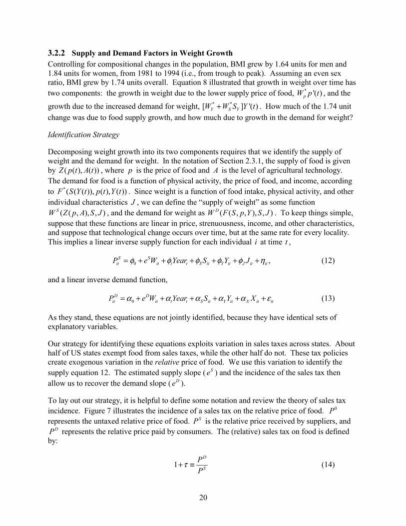
Our strategy for identifying these equations exploits variation in sales taxes across states. About half of US states exempt food from sales taxes, while the other half do not. These tax policies create exogenous variation in the relative price of food. We use this variation to identify the supply equation 12. The estimated supply slope ( Se ) and the incidence of the sales tax then allow us to recover the demand slope ( De ).

To lay out our strategy, it is helpful to define some notation and review the theory of sales tax incidence. Figure 7 illustrates the incidence of a sales tax on the relative price of food. 0P represents the untaxed relative price of food. SP is the relative price received by suppliers, and

DP represents the relative price paid by consumers. The (relative) sales tax on food is defined by:

1D

SPP

τ+ ≡ (14)

21

The tax is the percent increase in the relative price of food that results from sales taxation. If foodτ represents the sales tax rate for food in percentage terms, and otherτ represents the rate for

all other goods, the relative tax can be expressed as:

food otherτ τ τ= − (15)

For example, if there is a four percent tax on food and a three percent tax on other goods, the relative price paid by consumers is one percent higher than what suppliers receive. If sales taxes are uniform on all goods, they do not affect relative prices.

In Figure 7, the incidence of the sales tax on suppliers, κ , is defined as:

0 S

SP P

Pκτ −= (16)

If supply is perfectly elastic, 0 SP P= , and this incidence is zero. In this case, the sales tax does not affect the price collected by suppliers, and one hundred percent of the tax is borne by consumers.

To recover κ and to identify the supply curve, we estimate the following equation jointly with the supply curve in equation 12:

0 ,Sit it S it J it Y it t t itP S J Y Yearγ κτ γ γ γ γ δ= + + + + + + (17)

While the supply and demand equations are not identified, equation 17 can be estimated jointly with the supply curve in equation 12 via three-stage least squares, because taxation appears in equation 17, but not in 12. Moreover, the coefficient on taxation is approximately equal to the incidence of tax on the supplier, κ . Equation 16 implies that the incidence equals the percent reduction in supply price generated by a one percentage point increase in the tax, or

ln Sd Pd

κτ

= .25 Since the relative supply price tends to be reasonably close to one (the yearly

means range between 0.99 and 1.01), we can employ the approximation that ln S Sd P dP≈ . This justifies our claim that the coefficient on relative taxation is approximately equal to κ .

Knowing κ and Se then implies the demand slope De . We will take advantage of this fact to identify the slope of the demand function, even without any instruments for the demand price. In particular, the geometry of Figure 7 implies that:

25 To estimate the proper incidence, we need to control for other factors that may be shifting demand—besides the sales tax—but we ought not to control for weight, since the change in price is accompanied by a change in equilibrium weight. Therefore, equation 17 includes demand shifters as regressors, but not weight.

22

1D Se eκκ−= − (18)

This approach yields an estimated supply slope ( Se ), shifts over time in the supply curve ( tφ ), sales tax incidence (κ ), and demand slope ( De ). These parameters can be used to decompose technological change into its supply and demand components.

Using the estimated shift over time in supply, we can estimate the portion of BMI growth generated by shifts in the supply of food. In particular, 1994 1981φ φ− represents the vertical shift in the inverse supply curve from 1981 to 1994. A simple geometric argument reveals that the resulting shift in BMI must be:

1994 1981 ,S DBMIe e

φ φ−∆ =−

(19)

where the coefficients tφ are taken from the inverse supply curve in equation 12. Similarly, the shift in equilibrium price that results is:

DP e BMI∆ = − ∆ (20)

We will be able to calculate both these quantities directly by estimating Se , De , and 1994 1981φ φ− .

Data

We construct a data set with individual weight and other characteristics, along with geographic identifiers that allow us to link individuals to data on relative prices and taxes for different localities. We use the NLSY Geocode data set, which provides geographic identifiers for each NLSY individual. Data are reported on the individual’s state of residence, and Standard Metropolitan Statistical Area (SMSA) of residence. We then compile data on relative food prices across SMSA’s, and data on taxation across states; these data are linked to the NLSY via the SMSA and state identifiers.

The first challenge is to construct price indices for food and other items that are comparable across states and across years. We employ data from the American Chamber of Commerce Researchers Association (ACCRA) on inter-city prices, as well as data from the Bureau of Labor Statistics (BLS) on price variation over time, within particular cities. We will use the 1989 ACCRA data, which provides price indices for about 200 metropolitan areas in the US. For the price of food, we will use their basket of “grocery goods,” but we exclude three non-food items: laundry detergent, facial tissue, and cigarettes, which together comprise about 15% of the ACCRA grocery bundle. This basket represents all food items purchased for consumption in the home. To construct price indices for non-food goods, we employ two different strategies. First, we construct a price index over all other goods in the ACCRA survey.26 However, since this

26 A small fraction—about 6%—of this bundle consists of food eaten at restaurants. We choose to keep these goods in the “non-food” bundle in order to focus on the price of food, rather than the demand for

23

includes some goods that are not subject to sales tax, we also construct an index for the price of non-food retail goods, all of which are subject to sales taxes. Relative prices will be constructed as the price of food relative to the price of all non-food goods, and alternatively as the price of food relative to non-food retail goods.

While the ACCRA data are comparable across cities in 1989, they are not comparable across years. Therefore, we extrapolate the cross-sectional data backwards and forwards by using data from the BLS on price variation within each city over time. The BLS collects price indices for 26 major metropolitan areas, for food at home and all items. These data are available for every year from 1979 to 1998. In addition to these 26 major areas, the BLS also constructs price indices by region (i.e., South, Northeast, Midwest, and West) and three city size classes. In the absence of BLS data for the specific city in question, we use the indices for the appropriate region and city size class. These indices are not comparable across cities, but they are comparable within cities and across years. Therefore, we use growth in the price of food at home to extrapolate our ACCRA food price series backwards to 1979 and forward to 1998. Similarly, we use growth in the BLS price index for “All Items” to do the same for the ACCRA non-food price indices. This yields a complete set of prices for all years of the NLSY, and across all metropolitan areas contained in the ACCRA data. The constructed series is comparable across cities and across time.

The ACCRA list of cities is similar, but not identical, to the NLSY’s list of SMSA’s. To link the ACCRA cities with the NLSY’s SMSA’s, we use the following rule. If an NLSY SMSA is not directly present in the ACCRA data, we link it to an ACCRA city within 100 miles driving distance of it (if several ACCRA cities meet that criterion, we use the closest one). If no ACCRA city is present within 100 miles, we leave the price data as missing.27

We obtain state sales tax data from a biennial28 publication by the Tax Foundation, entitled Facts and Figures on Government Finance. This publication reports state sales taxes, along with whether or not the state exempts food from taxation.29 We construct the relative taxation of food as food otherτ τ τ= − , where foodτ is the sales tax rate on food, and otherτ is the rate on other goods. In different contexts, other researchers have found that sales tax variation does explain price variation in the ACCRA data (Besley and Rosen 1999).

food preparation, and also because restaurant food is usually subject to the general rate of sales taxation, not the special rate for food (when it exists).

27 Driving distances are calculated using the MapQuest service, at www.mapquest.com.

28 More correctly, this publication is “slightly more than biennial”. Over our time period, it is available in: 1979, 1981, 1983, 1986, 1988/89, 1990-5 annually, 1997, and 1998. We linearly interpolate missing years.

29 In 1994, 1995, 1997, and 1998, the Tax Foundation did not report whether or not the state exempted food. For these years, we assume that state policies did not change, if it maintained the same policy for 1992 and 1993. In practice, all states had maintained consistent policies for at least these two preceding years.

24

The data on food prices and taxes are summarized in Table 5. From 1981 to 1994, all the price indices grew between fifty and sixty percentage points, although prices grew more rapidly for non-food items. The relative price of food (before sales taxes) fell by nearly eight percentage points over the same period of time. Concurrent with this decline, the relative tax imposed on food fell by about 0.5 percentage points.

Results

The estimates of equations 17 and 12 are presented in Table 6, for three different specifications. The first two specifications use the price of food relative to all non-food items as the dependent variables. The first is the most parsimonious specification. The supply function is identified by relative taxation. Income decile dummies are not included in the supply equation results, because they turn out to be uniformly insignificant for the supply of weight. This initial specification implies that the slope of the inverse supply function is 0.56. A one-unit increase in BMI raises the supply price by about half a percentage point. Conversely, a one percent increase in the relative price raises BMI by about 2 units. Since average BMI is around 25 in the population, this corresponds to a supply elasticity of around eight, which is quite an elastic supply response. In contrast, demand is relatively inelastic. A one percent change in the relative price lowers BMI by only 0.168 units, or 0.6 percent. In fact, this elasticity of 0.6 is the highest of any we estimate. The elasticity of the supply curve is reflected in the estimated tax incidence: only ten percent of the tax is borne by producers. Finally, this initial specification suggests that, holding BMI constant, the supply curve shifted down by 6.18 percentage points from 1981 to 1994. This would have translated into a 0.95 unit increase in BMI and would have accounted for about 55% of the secular growth in BMI from 1981 to 1994. This is the largest estimate we get for the effect of supply growth on weight. Significantly, this percentage estimate, like all the other percentage estimates to follow, does not change if we examine other periods besides 1981-1994.

The second specification allows for the fact that changes in educational or racial composition can affect weight, holding the price of food constant. This generalization does not affect the slope of the supply curve, but it does lower the estimated slope of the demand curve by about 25 percent, to 0.12. The estimated demand elasticity falls even further, to a value of less than 0.5. This specification implies that supply growth raised BMI by 0.72 units from 1981 to 1994, or about 41% of the total 1.2 unit growth.

One drawback of our approach is that the coefficients on the variables besides prices and taxes have no obvious interpretation. The coefficients in the first-stage regression do not represent the effect of each variable on demand: the first-stage regression is not a demand equation, because BMI is not included in it. The coefficients in the supply regression can be interpreted either as shifters of food supply, or as reflecting preferences for weight. For example, the fact that Hispanics face lower relative food prices can be interpreted in one of two ways. First, it could be that the proportion of Hispanic workers is correlated with a larger agricultural labor force and a greater supply of food. Alternatively, it could be that Hispanics weigh more at constant food prices, because they have greater preferences for weight. We cannot disentangle these two interpretations.

25

The final specification repeats this last analysis using a different measure of relative prices: we compute the price of food relative to the price of non-food retail items. This is likely to be a more precise strategy for estimating tax incidence, since sales taxes are only applied to retail items. It is encouraging that the change in the measurement of prices, while it does affect some coefficients, leaves the supply-induced growth in BMI virtually unchanged, at around 0.74 units, or around 43% of the total growth. The estimated incidence of sales tax on the producer falls with the change in measurement, to around three percent, but the estimated slope of the supply curve falls by roughly the same percentage. This leaves the total estimated BMI growth unchanged. This analysis demonstrates that mismeasurement of taxation—we do not observe effective tax rates on non-retail items like housing and utilities—does not affect our conclusion that about forty percent of the growth in BMI arose from expansions in the supply of food.

4 Conclusion This paper provided a theoretical and empirical examination of the forces that have been contributing to the long-run growth in weight over time. We considered the hypothesis that technological change has led to weight growth by making home- and market-production more sedentary and by lowering food prices through agricultural innovation. We also derived the peculiar relationships among income, weight, and food prices that obtain in the presence of such technological change. We used microdata from a variety of sources to quantify the importance of job-related exercise in weight determination, and found it to be significant. We also decomposed the growth in weight over the last few decades and find that about forty percent of it may be due to expansion in the supply of food, potentially through agricultural innovation, and about sixty percent due to demand factors such as a fall in physical activity in market-and home production.

The paper suggests several avenues of future research. First, the sources of growth in weight need to be better understood to improve policy responses to the rising epidemic of obesity. Currently, the major public interventions against obesity involve education programs emphasizing the benefits of good diet and exercise. However, if technological change in production is the major factor driving the trend, information may be less of an issue than incentives. Indeed, we may have become more informed over time as weight has increased.

Second, an aspect of technological change we began to explore in the empirical work concerns changes in the price of food. It remains to show exactly why the relative supply price of food seemed to decline, particularly during the early 1980s. More detailed analysis of technological change in agricultural production seems to be the logical next step in a research agenda that aims to understand the economics of weight gain.

Third, although the analysis here stresses the impact of technological change on the quantity of food and calorie consumption, it may have affected the quality of food intake as well. In particular, technological advances may have affected the relative prices of the different sources of calories such as proteins and fats. It is interesting to note that the food diary data from the National Health and Nutrition Examination Surveys suggests that the proportion of calories from fat actually fell slightly during the 1980s. Nonetheless, a substantial increase in total calories consumed pushed up total fat intake. Therefore, it seems important to understand the interaction

26

between quantity and quality, particularly to better understand the negative relationship between income and weight induced by high-calorie foods being less expensive.

Fourth, a better understanding is needed of the relative importance of labor- versus leisure activities in the impact technological change has had in reducing activity levels. Leisure issues are particularly important for understanding the growth in child obesity that may be due to technological change, such as computers and television, which have raised the utility of consuming leisure but lowered the calories spent in doing so. Although few data sets will likely be available to do so on a population bases, one may potentially pursue the empirical strategy of identifying a control profession for which the calories spent per hour worked has not changed over time, and using its weight growth as a measure of the impact of technological change in leisure on weight.

Finally, although existing data do not allow for a clean, systematic, and convincing decomposition of weight growth into a food component and an exercise component, future data production aimed at collecting micro-data on occupation, demographics, and food consumption could make such analysis feasible. This would further advance our understanding of the relationship between weight and technological change.

27

References Araujo, A. (1991). “The Once But Not Twice Differentiability of the Policy Function.”

Econometrica 59(5): 1383-93.

Behrman, Jere R., and M. R. Rosenzweig (2001). “The Returns to Increasing Body Weight,” Mimeo, University of Pennsylvania.

Besley, Timothy J., and H. S. Rosen (1999). “Sales Taxes and Prices: An Empirical Analysis,” National Tax Journal, 52(2): pp. 157-178.

Bound, John, C. Brown, and N. Mathiowetz (1999). “Measurement Error in Survey Data,” Handbook of Econometrics, volume 4. Eds., James Heckman and Edward Leamer. New York: Springer-Verlag.

Cawley, John (2000). “Body Weight and Women’s Labor Market Outcomes,” Working Paper No. 7841, National Bureau of Economic Research. Cambridge, MA: National Bureau of Economic Research.

Cawley, John (1999). Obesity and Addiction. Ph.D. Dissertation, Department of Economics, The University of Chicago.

Chou, Shin-Yi, Michael Grossman, and Henry Saffer (2001). “An Economic Analysis of Adult Obesity: Results from the Behavioral Risk Factor Surveillance System.” Working Paper, City University of New York Graduate Center.

Costa, Dora, and R. Steckel (1995). “Long-Term Trends in Health, Welfare, and Economic Growth in the United States,” NBER Historical Working Paper No. 76. Cambridge, MA: National Bureau of Economic Research.

Department of Labor. Bureau of Labor Statistics (1986). Dictionary of Occupational Titles, Fourth Edition. Springfield, VA: National Technical Information Service. [computer file]

England, Paula and B. Kilbourne (1998). Occupational Measures from the Dictionary of Occupational Titles for 1980 Census Detailed Occupations. Ann Arbor, MI: Inter-university Consortium for Political and Social Research. [computer file]

Hamermesh, Daniel S., and J. E. Biddle (1994). “Beauty and the Labor Market,” American Economic Review, 84(5): pp. 1174-94.

Keeler, E., W. Manning, J. Newhouse, E. Sloss, and J. Wasserman (1989). “The External Costs of a Sedentary Life-style,” American Journal of Public Health, 79(8): pp. 975-81.

Loh, Eng Seng (1993). “The Economic Effects of Physical Appearance,” Social Science Quarterly, 74(2): pp. 420-438.

28

Philipson, Tomas J., (2001), “The World Wide Growth in Obesity: An Economic Research Agenda”, Health Economics, v 10, p 1-7.

Philipson, Tomas J. and R. A. Posner (1999). “The Long-Run Growth in Obesity as A Function of Technological Change,” Working Paper No. 7423, National Bureau of Economic Research. Cambridge, MA: National Bureau of Economic Research.

Poterba, James M. (1996). “Retail Price Reactions to Changes in State and Local Sales Taxes,” National Tax Journal, 49(2): pp. 165-176.

Putnam, Judith Jones, and Jane E. Allshouse (1999). “Food Consumption, Prices, and Expenditures, 1970-97.” Food and Rural Economic Division, Economic Research Service, US Department of Agriculture. Statistical Bulletin No. 965.

Register, C. A. and D. R.Williams (1990). “Wage Effects of Obesity Among Young Workers,” Social Science Quarterly, 71(1): pp. 130-41.

Strauss, John, and T. Duncan (1995). “Human Resources: Empirical Modeling of Household and Family Decisions,” Handbook of Development Economics: Volume 3A. Handbooks in Economics, vol. 9. New York: Elsevier Science, pp. 1883-2023.

Tuomilehto, Jaakko, et al. (2001). “Prevention of Type 2 Diabetes Mellitus by Changes in Lifestyle among Subjects with Impaired Glucose Tolerance,” New England Journal of Medicine, 344(18, May 3): pp. 1343-50.

Wolf, Anne, and G. Colditz (1998). “Current Estimates of The Economic Cost of Obesity in The United States,” Obesity Research, 6(2): pp. 97-106.

1982 1998 1982 1998BMI 23.5 26.9 22.1 26.2Obesity 0.05 0.22 0.05 0.27Age 20.7 37.0 20.7 37.0Black 0.14 0.14 0.14 0.14Hispanic 0.06 0.07 0.06 0.06Married 0.17 0.63 0.30 0.66Highest Grade Attained 12.0 13.4 12.2 13.4Distribution of StrengthRequirements:

Strength=1 0.307 0.256 0.419 0.357Strength=2 0.589 0.672 0.479 0.574Strength=3 0.058 0.041 0.087 0.051Strength=4 0.044 0.029 0.015 0.017Strength=5 0.003 0.002 0.000 0.001

Distribution ofJob-Related Exercise:

Strenuousness=0 0.435 0.373 0.436 0.398Strenuousness=1 0.482 0.570 0.545 0.593Strenuousness=2 0.019 0.030 0.004 0.004Strenuousness=3 0.064 0.027 0.015 0.006

Source: NLSY, 1982-1998.

Working Men Working Women

Table 1: Summary Statistics for NLSY, 1982-1998.

S -0.35 *3.64

Muscle 0.33 *4.23

S Stock -1.22 * -0.19 *2.49 1.99

Muscle Stock 0.94 * 0.16 *2.51 2.06

Highest Grade Completed -0.16 * -0.12 * -0.035.02 2.01 1.11

Black 2.63 * 3.73 *13.71 11.32

Hispanic 1.10 * 1.48 *5.24 4.01

Married -0.09 -0.18 0.59 *0.73 0.64 12.95

Age 0.45 * 3.08 .4.47 1.68 .

Age Squared -0.005 * -0.04 .-2.34 -1.57 .

Wage Decile 1d 0.00 0.00 0.00. . .

Wage Decile 2 -0.12 -0.33 -0.20 *0.47 0.65 1.99

Wage Decile 3 -0.11 -0.02 -0.21 *0.65 0.03 2.81

Wage Decile 4 0.07 -0.13 -0.29 *0.37 0.24 3.96

Wage Decile 5 -0.26 -0.34 -0.26 *1.45 0.63 3.36

Wage Decile 6 -0.19 -0.23 -0.36 *1.03 0.42 4.61

Wage Decile 7 -0.35 ** -0.59 -0.43 *1.83 1.08 5.33

Wage Decile 8 -0.49 * -0.77 -0.44 *2.43 1.28 5.21

Wage Decile 9 -0.86 * -1.64 * -0.50 *4.18 2.65 5.51

Wage Decile 10 -1.05 * -1.56 * -0.52 *4.39 2.40 4.72

Constant 16.61 * -29.81 23.09 *12.93 0.93 70.18

Year Effects Yes No YesObservations 33655 2358 31344R-squared 0.12 0.09 0.22Robust t-statistics in parentheses*Significant at the 95% level.**Significant at the 90% level.aStandard errors are clustered by individual.bIncludes only 1996 observations.cIncludes person-level fixed-effects.dIndicates excluded group.

Fixed-EffectscPooleda 1996b

Table 2: Effects of Occupation on Weight for Working Women in the NLSY.

1976 1994 1976 1994BMI 24.93 26.19 23.12 24.65Obesity 0.090 0.168 0.090 0.171Age 38.568 38.469 37.109 38.625Black 0.083 0.100 0.113 0.123Married, Spouse Present 0.739 0.682 0.585 0.619Highest Grade Attained 12.231 13.233 12.334 13.369Distribution of StrengthRequirements:*

Strength=1 0.137 ** 0.175 0.315 ** 0.341Strength=2 0.446 ** 0.412 0.478 ** 0.445Strength=3 0.289 ** 0.290 0.178 ** 0.179Strength=4 0.123 ** 0.118 0.029 ** 0.036Strength=5 0.005 ** 0.005 0.000 ** 0.000

Distribution ofJob-Related Exercise:†

Strenuousness=0 0.300 ** 0.271 0.255 ** 0.308Strenuousness=1 0.480 ** 0.436 0.616 ** 0.577Strenuousness=2 0.226 ** 0.242 0.090 ** 0.078Strenuousness=3 0.129 ** 0.119 0.038 ** 0.037

Source: NHIS, 1976-1994.*From 1983 to 1994, Strength is rated on a continuous, non-integerscale, from 1 to 5. To derive these statistics, the interval from 1 to 5 is split into five equal intervals of 0.8 units each. For example, the Strength=1 category corresponds to a score between 1 and 1.8.**Indicates 1983 value.†From 1983 to 1994, Strenuousness is rated on a continuous, non-integerscale, from 0 to 3. To derive these statistics, the interval from 0 to 3 is split into four equal intervals of 0.75 units each. For example, the Strenuousness=0 category corresponds to a score between 0 and 0.75.

Working Men Working Women

Table 3: Trends in Weight and Occupation in the NHIS, 1976-1994.

Dependent Variable:Adjusted BMI Coefficient T-Statistica Coefficient T-Statistica

S -0.209 * 16.71 -0.102 * 5.17Muscle 0.225 * 17.06 0.432 * 28.52Income Quartile 1 -0.218 * 10.83 0.322 * 12.65Income Quartile 2b 0 . 0 .Income Quartile 3 0.025 1.52 -0.488 * 22.22Income Quartile 4 -0.078 * 4.27 -0.908 * 37.61Age 0.283 * 102.13 0.321 * 87.26Age Squared -0.003 * 89.91 -0.003 * 65.95Highest Grade Completed -0.107 * 43.19 -0.221 * 60Year=1976 -1.036 * 29.21 -1.201 * 25Year=1977 -0.92 * 17.35 -1.087 * 15.31Year=1978 -0.875 * 24.2 -1.221 * 25.57Year=1979 -0.913 * 25.16 -1.136 * 23.57Year=1980 -0.841 * 22.69 -1.12 * 22.78Year=1981 -1.338 * 33.93 -2.142 * 40.62Year=1982 -0.743 * 20.24 -0.817 * 16.84Year=1983 -0.702 * 19.06 -0.912 * 18.84Year=1984 -0.948 * 22.13 -2.344 * 41.92Year=1985 -0.528 * 13.62 -0.679 * 13.29Year=1986 -0.423 * 9.75 -0.546 * 9.69Year=1987 -0.374 * 10.1 -0.44 * 9.11Year=1988 -0.306 * 8.31 -0.368 * 7.71Year=1989 -0.153 * 4.03 -0.253 * 5.15Year=1990 -0.106 * 2.79 -0.191 * 3.93Year=1991b 0 . 0 .Year=1992 0.162 * 4.04 0.177 * 3.47Year=1993 0.219 * 5.19 0.197 * 3.69Year=1994 0.306 * 7.63 0.3 * 5.7Northeast -0.008 0.44 0.017 0.73North-Central 0.109 * 6.51 0.293 * 13.03SouthWest -0.358 * 20.65 -0.179 * 7.78Black 0.109 * 4.44 1.997 * 66.78Married, Spouse Present 0.655 * 41.05 -0.055 * 2.82Constant 20.306 * 277.97 19.404 * 207.26Observations 439628 361332R-Squared 0.08 0.12*Significant at 99% Level.**Significant at 95% Level.aBased on robust standard errors.bIndicates omitted category.

FemalesMales

Table 4: Regression Results for NHIS, 1976-1994.

Table 5: Summary of Data on Prices and Taxes.

1981 1989 1994Price Index: 76.9 100.2 126.1167 Food Items in Grocery Basket 4.3 5.6 6.871135

Price Index: 74.4 101.1 139.8255 All Non-Food Items 7.8 11.7 20.53401

Price Index: 74.1 100.6 130.9597 Retail Non-Food Items 4.4 5.7 8.133273

Price Index: 74.5 101.3 138.4168 All Items 7.1 10.6 18.14214

Relative Price of Food: 1.042 1.00 0.966 Grocery Food Items/All Non-Food 0.10 0.09 0.08

State Sales Tax on Food 2.2 3.4 2.82.4 2.5 2.8

State Sales Tax on non-Food 3.6 4.7 4.71.6 1.1 1.8

Relative Tax: -1.4 -1.7 -1.9 Food Tax Minus non-Food Tax 1.8 2.2 2.5Notes: Standard deviations appear below means. Means are computedacross SMSA's for price data, and across states for tax data.

Table 6: Estimated Supply and Demand Functions for BMI.

Dependent Variable:

Adjusted BMI: 1/eS 0.56 * 0.57 * 0.29 *0.10 0.15 0.08

Shift in Inverse Supply -6.18 * -6.32 * -6.51 * Curve: φ1994-φ1981 0.48 0.67 0.36

Relative Tax: κ -0.10 * -0.07 * -0.03 *0.010 0.010 0.005

Highest Grade Attained 0.07 ** 0.00 0.08 * 0.04 *0.04 0.02 0.02 0.01

Black 1.23 * 1.18 * -0.15 -0.160.22 0.21 0.12 0.11

Female 0.41 * 0.59 ** 0.51 ** 0.13 0.110.11 0.24 0.24 0.13 0.13

Black*Female -0.32 0.91 * 0.13 0.73 *0.47 0.28 0.26 0.16

Hispanic -6.25 * -5.81 * -4.63 * -4.41 *0.22 0.19 0.12 0.11

Hispanic*Female 1.35 * 1.58 * 0.73 * 0.84 *0.29 0.26 0.16 0.14

Income Decile no yes no yes no yes

Income Decile*Female no yes no yes no yes

Year yes yes yes yes yes yes

Pseudo R-Squared 0.00 0.03 0.03 0.07 0.12 0.15Slope of Demand: eD * * *

Supply-Induced BMI Growth, 1982-94Observations*Significant at 1% level.**Significant at 5% level.Note: Generalized Least Squares standard errors appear below coefficients. These are robust to correlation within individuals in the panel.

Relative to Retail Non-Food

46994

0.1170.039

0.74

Supply StageInverse First-

49628

0.1680.035

0.95

46994

0.1210.036

0.72

Food Price Relative to All Non-FoodInverseSupply

First-Stage

InverseSupply

First-Stage

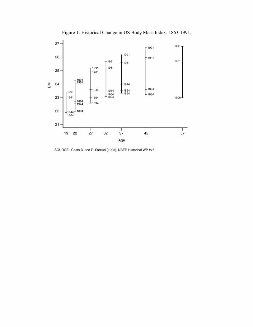
Figure 1: Historical Change in US Body Mass Index: 1863-1991.

19 574537322722

Age

27

21

22

23

24

25

26

BM

I

1991

1961

19441864

19911961

1944

1894

1864

19911961

1944

1894

1864

1991

1961

1944

18941864

1991

1961

1944

18941864

1991

1961

1894

1991

1961

19001864

SOURCE: Costa D. and R. Steckel (1995), NBER Historical WP #76.

19391919 19291909 1949 1959 1969 1979 1989 1998

Source: USDA’s Economic Research Service

Calories Available From the Food Supply per Person per Day,

1909 - 1998Calories Available

Calories per person per day

Total Food Supply

Food supply adjusted for spoilage and waste

4,000

3,500

3,000

2,500

2,000

Figure 2: Long-Run Changes in Calorie Consumption.

Figu

re 3

: Cha

nges

in th

e R

elat

ive

Pric

e of

Foo

d in

the

US,

195

1-20

00.

0.96

0.981

1.02

1.04

1.06

1.081.

1

1.12

1.14

1940

1950

1960

1970

1980

1990

2000

2010

Year

Relative Price of FoodBLS Food Price Index Deflated by Overall CPI

Raw

Pric

e D

ata

Line

ar T

ime

Tren

d

Figu

re 4

: Ste

ady-

Stat

e W

eigh

t and

Foo

d C

onsu

mpt

ion.

F

W

F(W

;S)

Φ(W

;S,p

,Y) W

*Φ

>FG

ain

Wei

ght

Φ<F

Lose

Wei

ght

F*

Figu

re 5

: Rep

ortin

g B

ias i

n W

eigh

t Dat

a, b

y Se

x an

d R

ace.

-10-8-6-4-2024

4050

6070

8090

100

110

120

130

140

Rep

orte

d W

eigh

t (K

ilogr

ams)

Reporting Bias (Kilograms)

Whi

te M

enN

on-W

hite

Men

Whi

te W

omen

Non

-Whi

te W

omen

-2.0

0

-1.0

0

0.00

1.00

2.00

3.00

4.00

12

34

56

78

910

Wag

e D

ecile

BMI Relative to Bottom Decile

Inco

me

Effe

ctSt

renu

ousn

ess

Effe

ctC

ombi

ned

Effe

ct

Figu

re 6

: Tim

e Pa

th o

f Wei

ght w

ith L

inea

r R

educ

tion

in S

tren

uous

ness

.

Pd

Ps

P0

BMI

D

S

Figure 7: Incidence of a Sales Tax on Food.