NBER WORKING PAPER SERIES

THE INEXORABLE AND MYSTERIOUS TRADEOFFBETWEEN INFLATION AND UNEMPLOYMENT

N. Gregory Mankiw

Working Paper 7884http://www.nber.org/papers/w7884

NATIONAL BUREAU OF ECONOMIC RESEARCH1050 Massachusetts Avenue

Cambridge, MA 02138September 2000

This paper was prepared as the Harry Johnson Lecture at the annual meeting of the Royal EconomicSociety, July 2000. I am grateful to Larry Ball, Olivier Blanchard, Julio Rotemberg, and JustinWolfers for comments. The views expressed herein are those of the author and not necessarily those of theNational Bureau of Economic Research.

2000 by N. Gregory Mailkiw. All rights reserved. Short sections of text, not to exceed two paragraphs,may be quoted without explicit permission provided that full credit, including notice, is given to thesource.

The Inexorable and Mysterious Tradeoff Between Inflation and UnemploymentN. Gregory MankiwNBER Working Paper No. 7884September 2000

ABSTRACT

This paper discusses the short-mn tradeoffbetween inflation and unemployment. Although this

tradeoff remains a necessary building block of business cycle theory, economists have yet to provide

a completely satisfactory explanation for it. According to the consensus view among central bankers

and monetary economists, a contractionary monetary shock raises unemployment, at least temporarily,

and leads to a delayed and gradual fall in inflation. Standard dynamic models of price adjustment,

however, carmot explain this pattern of responses. Reconciling the consensus view about the effects

of monetary policy with models of price adjustment remains an outstanding puzzle for business cycle

theorists.

N. Gregory MankiwDepartment of EconomicsLittauer 223Harvard UniversityCambridge, MA 02138and NBERngmankiw@harvard.edu

Several years ago I gave myself a peculiar assignment: I decided to try to summarize all

of economics in ten simply stated principles. The purpose of this task was to introduce students

to the economic way of thinking in the first chapter of my textbook Principles of Economics.

I figured if God could boil all of moral philosophy down to ten commandments, I should be able

to do much the same with economic science.

Most of the ten principles I chose were microeconomic and hard to argue with. They

involved the importance of tradeoffs, marginal analysis, the benefits of trade, market efficiency,

market failure, and so on. I allocated the last three principles to macroeconomics. The first of

these was "A country's standard of living depends on its ability to produce goods and services,"

which I viewed as the foundation of all growth theory. The second was, "Prices rise when the

government prints too much money," which I took to be the essence of classical monetary

theory. The last of my ten principles is the subject of today's lecture: "Society faces a short-run

tradeoff between inflation and unemployment."

Perhaps not surprisingly, this statement turned out to be controversial. When my

publisher sent out the manuscript for review, a few readers objected to this principle on the

grounds that the inflation-unemployment tradeoff was still a speculative idea. Since my book

came out, I have sometimes been asked whether I am going to revise this principle in light of

recent experience. The combination of low inflation and low unemployment enjoyed by the

United States in the late 1990s suggests to some people that there is no longer a tradeoff between

these two variables, or perhaps that it never existed at all.

My goal in this lecture is to discuss our current understanding of the inflation-

1

unemployment tradeoff. My views in this matter are summarized by the two adjectives in my

title: inexorable and mysterious. The tradeoff is inexorable because it is impossible to make

sense of the business cycle, and in particular the short-mn effects of monetary policy, unless we

admit the existence of a tradeoff between inflation and unemployment. That's why I included

this tradeoff as one of the ten essential principles of economics. The tradeoff remains

mysterious, however, for the economics profession has yet to produce a satisfactory theory to

explain it. Indeed, the standard models of inflation-unemployment dynamics are inconsistent

with conventional views about the effects of monetary policy. Resolving this inconsistency is

a prominent outstanding puzzle for business cycle theorists.

What is the inflation-unemployment tradeoff!

Let me start be trying be precise about what I mean when I say there is a tradeoff

between inflation and unemployment. I do not mean that a scatterplot of these two variables

produces a stable downward-sloping Phillips curve. Nor do I mean that any particular regression

fits the data well or produces any particular set of coefficients. The inflation-unemployment

tradeoff is, at its heart, a statement about the effects of monetary policy. It is the claim that

changes in monetary policy push these two variables in opposite directions.

There is, of course, a long tradition suggesting that such a tradeoff exists and that it holds

only in the short run. In his 1752 essay "Of Money," David Hume wrote the following:

In my opinion, it is only in the interval or intermediate situation, between the acquisition

of money and the rise in prices, that the increasing quantity of gold or silver is

favourable to industry. . . . The farmer or gardener, finding that their commodities are

2

taken off, apply themselves with alacrity to the raising of more. . . . It is easy to trace

the money in its progress through the whole commonwealth; where we shall find that it

must first quicken the diligence of every individual, before it increases the price of

labour.

This is an amazing quotation. It shows that this basic lesson of business cycle theory has been

understood for well over two centuries. Notice Hume's emphasis on the timing: A monetary

injection first increases output and employment, and later increases the price level. I will return

to this issue shortly.

At limes, some economists have downplayed monetary nonneutrality--the real business

cycle theorists of the 1980s being a prominent example. But those holding this alternative view

are a minority, both historically and today. Most current researchers building on the real

business cycle tradition embrace its emphasis on explicit dynamic, stochastic general equilibrium

models but are leaving behind the premise of monetary neutrality. Indeed, they often include

sticky prices as a source of nonneutrality. (See, e.g., Goodfriend and King, 1997.) There is

now a broad consensus that Hume was right: Monetary policy affects both nominal variables

such as inflation and real variables such as unemployment. The challenge facing business cycle

theorists is to explain this fact.

The Phillips Curve As an Empirical Proposition

Before turning to the theory, let me say a few words about the large body of empirical

work on inflation-unemployment dynamics. There is a range of opinion about this topic. On

the one hand, Robert Lucas and Thomas Sargent (1978) claimed in their manifesto "After

3

Keynesian Macroeconomics" that the breakdown of the simple Phillips curve in the 1970s

exposed the bankruptcy of the prevailing Keynesian paradigm. In their words, it was

"econometric failure on a grand scale." On the other hand, many economists view the Phillips

curve augmented to include adaptive expectations and supply shocks as a remarkably stable

relationship. Alan Blinder (1997) has called the reliability of the modem Phillips curve the

"clean little secret" of macroeconomics.

My own view is between these two extremes. It is hard to argue that empirical Phillips

curve equations are easily estimated and completely reliable for forecasting and policy analysis.

There are all the issues involving expectations that Lucas (1976) put forth so famously. But

even if we put the Lucas critique aside, we run into the more mundane but equally important

problem that estimates of the natural rate of unemployment (or NAIRU, as it is sometimes

called) are far from precise.

One odd feature of the empirical literature on the modem Phillips curve is that it rarely

provides standard errors for estimates of the natural rate. A notable exception is a 1997 paper

by Douglas Staiger, James Stock, and Mark Watson. Using a conventional specification, they

estimated the U.S. natural rate in 1990 to be 6.2 percent, with a 95 percent confidence interval

from 5.1 to 7.7 percent. This large degree of uncertainty was greeted with skepticism at the

time. (See, e.g., Gordon, 1996). But no one has offered any reason to doubt their

econometrics, and the subsequent U.S. experience of low unemployment and surprisingly

dormant inflation confirms that the natural rate is impossible to know with much precision.

At the same time, it is also hard to argue that the empirical Phillips curve should be

relegated to the trashbin of intellectual history. In another recent article, Stock and Watson

4

(1999) examine various methods for forecasting inflation. They report, "Inflation forecasts

produced by the Phillips curve generally have been more accurate than forecasts based on other

macroeconomic variables, including interest rates, money, and commodity prices. These

forecasts can, however, be improved upon using a generalized Phillips curved based on measures

of real aggregate activity other than unemployment.'

The right conclusion about the empirical Phillips curve seems clear: The glass is both half

full and half empty. This is hardly surprising. A combination of supply shocks that are hard

to measure and structural changes in the labor market that alter the natural rate makes it unlikely

that any empirical Phillips curve will ever offer a tight fit.

How full we measure the glass to be, however, is not important. Regardless of our

judgment on the empirical Phillips curve, we cannot easily escape the conclusion that monetary

policymakers face a short-run tradeoff between inflation and unemployment. The only

alternative to acknowledging such a tradeoff is to deny monetary policy's ability to influence one

of these two variables, and that is a tough position to defend.

Hysteresis?

One question about which I remain agnostic is whether the natural rate hypothesis is true

or whether some form of hysteresis causes monetary shocks to have long-lasting effects on

unemployment. The classical dichotomy has great attraction as a tenet of long-run

macroeconomic theory, but I am given pause by two recent papers by Laurence Ball (1997,

t999) on the rise in European unemployment in the 1980s. In the first paper, Ball shows that

countries that with larger decreases in inflation and longer disinflationary periods experienced

5

larger increases in their natural rates of unemployment. In the second paper, he establishes the

link to monetary policy: Countries that failed to pursue expansionary monetary policy in the

early 1980s (as measured by changes in interest rates) experienced larger increases in their

natural rates than did countries that did pursue expansionary monetary policy.

Even U.S. time series offer some evidence for hysteresis. John Campbell and I argued

in a 1987 paper that shocks to U.S. real GDP are typically very persistent--a conclusion that I

still believe to be true. If the effects of monetary shocks are temporary, then this finding

suggests the importance of nonmonetary shocks, such as shifts in productivity. But another

possible explanation for this fact is that the natural rate hypothesis is wrong and that monetary

disturbances cause some type of hysteresis.

This interpretation gets some surprising support from a recent paper by Ben Bernanke

and Ilian Mihov (1998), called "The Liquidity Effect and Long-Run Neutrality." I say

"surprising" because the paper purports to provide evidence for the opposite conclusion--long-run

monetary neutrality. Bernanke and Mihov estimate a structural vector autoregression and present

the impulse response functions for real GDP in response to a monetary policy shock. (See their

Figure III.) Their estimated impulse response function does not die out toward zero, as is

required by long-run neutrality. Instead, the point estimates imply a large impact of monetary

policy on GDP even after ten years. Bernanke and Mihov don't emphasize this fact because the

standard errors rise with the time horizon. Thus, if we look out far enough, the estimated

impact becomes statistically insignificant. But if one does not approach the data with a prior

view favoring long-mn neutrality, one would not leave the data with that posterior. The data's

best guess is that monetary shocks leave permanent scars on the economy.

6

Theories of Monetary Nonneutrality

Let me now turn from empirics to theory--the main topic of this lecture. If one accepts

the view that monetary policy influences real variables such as unemployment, then explaining

this fact becomes a major challenge for economic theorists. Standard general equilibrium theory

gives no role for the unit of account. Indeed, the numeraire is normally irrelevant. In the

world, however, changes in the value of the unit of account (that is, inflation) seem to play a

big role in the allocation of resources. Why is that?

There have been many attempts to answer this question. Early work in the new classical

tradition emphasized imperfect information about prices, which leads people to confuse

fluctuations in the overall price level with fluctuations in relative prices (Lucas, 1973). Next

came a series of contributions emphasizing the slow adjustment of wages, perhaps due to formal

or implicit contracts between workers and firms (Fischer, 1977; Taylor, 1980). Then came

theories based on monopolistic competition in goods markets and costs of adjusting prices

(Rotemberg, 1982; Mankiw 1985; Akerlof and Yellen 1985; Blanchard and Kiyotaki 1987).

I won't go into detail about these approaches, in part because I have offered surveys

elsewhere (Ball, Mankiw, and Romer 1988; Mankiw, 1990; and Ball and Mankiw 1994). But

I will offer a few personal remarks about my own interest in theories based on monopolistically

competitive goods markets and sticky prices, as opposed to non-Walrasian labor markets and

sticky wages.

When I was first learning macroeconomics as a student of Alan Blinder in the late 1970s,

I was taught the sticky-wage theory of monetary nonneutrality as God's truth (or, to be more

precise, Keynes's truth--which in Alan's class was pretty much the same thing). Nominal wages

7

were slow to adjust, I was told, so when the central bank contracted the money supply and

prices fell, real wages rose, leading firms to lay off workers. Hence, we have a short-run

tradeoff between inflation and unemployment.

The problem with this story is that it is patently false. As the earliest critics of Keynes's

General Theory were aware, real wages do not exhibit the countercyclical behavior that this

theory predicts (Dunlop, 1938). This puzzle led me to start thinking about goods markets.

Maybe firms lay off workers after monetary contractions not because real labor costs are high

but because they can't sell all of the output they want. Prices, according to this story, are

failing to clear goods markets. But thinking about sticky prices naturally leads to analyzing

firms' decisions about price adjustment, which in turn forces us to think about firms with some

degree of market power, for competitive firms are price takers. In this way, the failure of real

wages to be countercyclical led me to be interested in the new Keynesian theory of monopolistic

competition and costly price adjustment.'

There is a close and interesting connection between this business cycle theory and anearlier set of theories that often go by the label "general disequilibrium." (Barro and Grossman,1971; Malinvaud, 1977). General disequilibrium theories took the vector of wages and pricesas given and then used the tools of general equilibrium analysis to examine the resultingallocation of resources. According to these theories, the economy can find itself in one ofseveral regimes, depending on which markets are experiencing excess supply and which areexperiencing excess demand. The most interesting regime--in the sense of corresponding bestto what we observe during recessions--is the "Keynesian" regime in which both the goods marketand the labor market exhibit excess supply. Unemployment arises because labor demand is low,which results because firms aren't selling all they want at prevailing prices.

One can view some New Keynesian theories as explaining why this particular regime ingeneral disequilibrium models is the normal case. When firms have market power, they chargeprices above marginal cost, so they always want to sell more at prevailing prices. In otherwords, if all firms have some degree of monopoly power, then goods markets are typically ina state of excess supply. This theory of the goods market is often married to a theory of thelabor market with above-equilibrium real wages, such as the efficiency-wage model. In thiscase, the "Keynesian" regime of generalized excess supply is not just one possible outcome for

8

Part of the appeal of these sticky-price models of the business cycle is the ample evidence

that prices really are sticky. In one comprehensive survey of U.S. firms, Alan Blinder (1994)

asked firms how often they change the prices of their major products. Naturally, the answers

show a lot of heterogeneity. But the median firm changes its prices once a year. In light of this

fact, it is not a stretch to suggest that sticky prices are one source of monetary nonneutrality.

In one sense, therefore, the short-run tradeoff between inflation and unemployment is

well understood: It arises from short-run price stickiness, which we can explain theoretically and

observe empirically. In another sense, however, the inflation-unemployment relationship

remains a mystery. In particular, once we leave behind static models of price adjustment and

try to develop a dynamic model, we run into some serious and still unresolved problems. Those

problems are the topic for the rest of this lecture.

Dynamic Price Adjustment: The New Keynesian PhilliDs Curve

There are two basic approaches to building dynamic models of price adjustment. One

approach is to assume that firms follow state-contingent rules--that is, they can adjust prices at

any time if they deem it profitable to do so given the costs of adjustment. The second approach

is to assume that firms follow time-contingent rules--that is, they adjust prices on a schedule,

perhaps determined optimally for the environment they face. There has been some small but

significant theoretical advances on state-contingent adjustment (most notably, Caplin and

Spulber, 1987; Caplin and Leahy, 1991), but most recent work on price dynamics assumes that

the economy, but the typical one.

9

adjustment is time-contingent. This may be for no better reason than that this assumption makes

the models easier to solve.

The specific model that has received the most attention over the past few years has been

dubbed the "new Keynesian Phillips curve." This model of inflation and unemployment can be

viewed as a dynamic extension of the static new Keynesian models of price adjustment I just

discussed. It has its intellectual antecedents in John Taylor's (1980) work on overlapping

contracts and Julio Rotemberg's (1982) model of quadratic costs of price adjustment. The most

elegant formulation is based on Guillermo Calvo's (1983) model of random price adjustment,

and that's the version I will sketch out for you here. Most of what I have to say about this

model, however, applies equally well to these other formulations, since they all yield the same

reduced-form relationship.2

In the Calvo model, firms follow time-contingent price adjustment rules. The time for

price adjustment does not follow a deterministic schedule, however, but arrives randomly.

Every period, a fraction X of firms adjust prices. Each firm has the same probability of being

one of the adjusting firms, regardless of how long it has been since its last price adjustment.

The assumption that price adjustment arrives as a Poisson process is not entirely realistic, but

it greatly simplifies the algebra, and it yields results qualitatively similar to what we would get

from more realistic assumptions with much more work.

To derive the new Keynesian Phillips curve, we start with three basic relationships. The

first concerns the firm's desired price, which is the price that would maximize profit at that

moment in time. With all prices expressed in logs, the desired price is:

2 For more on this equivalence, see Roberts (1995).

10

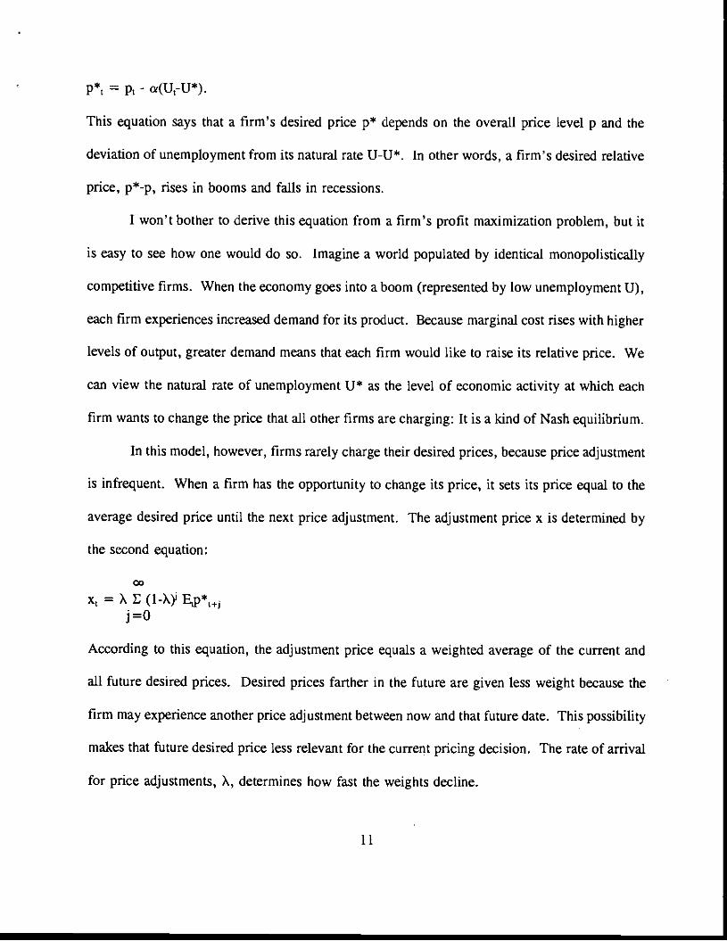
p* = p, -

This equation says that a firm's desired price p* depends on the overall price level p and the

deviation of unemployment from its natural rate In other words, a firm's desired relative

price, pp, rises in booms and falls in recessions.

I won't bother to derive this equation from a firm's profit maximization problem, but it

is easy to see how one would do so. Imagine a world populated by identical monopolistically

competitive firms. When the economy goes into a boom (represented by low unemployment U),

each firm experiences increased demand for its product. Because marginal cost rises with higher

levels of output, greater demand means that each firm would like to raise its relative price. We

can view the natural rate of unemployment U* as the level of economic activity at which each

firm wants to change the price that all other firms are charging: It is a kind of Nash equilibrium.

In this model, however, firms rarely charge their desired prices, because price adjustment

is infrequent. When a firm has the opportunity to change its price, it sets its price equal to the

average desired price until the next price adjustment. The adjustment price x is determined by

the second equation:

= X E (l-X Ep*1j=C)

According to this equation, the adjustment price equals a weighted avenge of the current and

all future desired prices. Desired prices farther in the future are given less weight because the

firm may experience another price adjustment between now and that future date. This possibility

makes that future desired price less relevant for the current pricing decision. The rate of arrival

for price adjustments, X, determines how fast the weights decline.

11

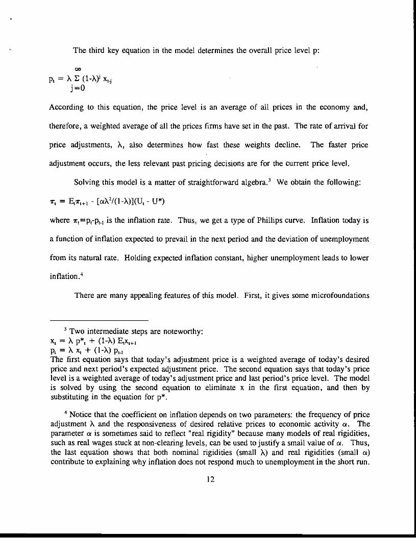
The third key equation in the model determines the overall price level p:

00

p1=X(l-XYx1j=o

According to this equation, the price level is an average of all prices in the economy and,

therefore, a weighted average of all the prices firms have set in the past. The rate of arrival for

price adjustments, X, also determines how fast these weights decline. The faster price

adjustment occurs, the less relevant past pricing decisions are for the current price level.

Solving this model is a matter of straightforward algebra.3 We obtain the following:

= Er÷1 - [aX2/(l-X)](U1 - U*)

where t=PrPt-i is the inflation rate. Thus, we get a type of Phillips curve. Inflation today is

a function of inflation expected to prevail in the next period and the deviation of unemployment

from its natural rate. Holding expected inflation constant, higher unemployment leads to lower

inflation.4

There are many appealing features of this model. First, it gives some microfoundations

Two intermediate steps are noteworthy:= X p* + (1-X) E1x÷1

p = X; + (1-A) ptThe first equation says that today's adjustment price is a weighted average of today's desiredprice and next period's expected adjustment price. The second equation says that today's pricelevel is a weighted average of today's adjustment price and last period's price level. The modelis solved by using the second equation to eliminate x in the first equation, and then bysubstituting in the equation for p.

Notice that the coefficient on inflation depends on two parameters: the frequency of priceadjustment A and the responsiveness of desired relative prices to economic activity a. Theparameter a is sometimes said to reflect "real rigidity" because many models of real rigidities,such as real wages stuck at non-clearing levels, can be used to justify a small value of a. Thus,the last equation shows that both nominal rigidities (small A) and real rigidities (small a)contribute to explaining why inflation does not respond much to unemployment in the short run.

12

to the idea that the overall price level adjusts slowly to changing economic conditions. Second,

it produces an expectations-augmented Phillips curve loosely resembling the model that Milton

Friedman and Edmund Phelps pioneered in the l960s and that remains the theoretical benchmark

for inflation-unemployment dynamics. Third, it is simple enough to be useful for theoretical

policy analysis. As a result, this model has become the workhorse for much recent research on

monetary policy. The recent survey article by Richard Clarida, Jordi Gali, and Mark Gertler

(1999) is one example, but it would be easy to cite many others. Bennett McCallum (1997) has

called this model "the closest thing there is to a standard specification."

Although the new Keynesian Phillips curve has many virtues, it also has one striking

vice: It is completely at odds with the facts. In particular, it cannot come even close to

explaining the dynamic effects of monetary policy on inflation and unemployment. This harsh

conclusion shows up several places in the recent literature, but judging from the continued

popularity of this model, I think it's fair to say that its fundamental inconsistency with the facts

is not widely appreciated. So I want to spend some time discussing the empirical problems with

this model and to describe them in a new and (I hope) more transparent way.

The Failure of the New Keynesian PhilliDs Curve I:

Disinflationary Booms

An early clue that there might be a problem with this model is in Laurence Ball's 1994(a)

paper "Credible Disinflation with Staggered Price Setting," which in turn built on some ideas

developed in 1978 by Edmund Phelps. Ball works with a standard Taylor-style overlapping

contract model (which, as I have noted, is analytically similar to the Calvo model I just

13

presented). He shows that a fully credible disinflation can cause an economic boom. The

reason is that price setters are forward-looking in this model. If a disinflation is announced and

is credible, firms should reduce the size of their price hikes even before the money supply

slows. As a result, real money balances rise, leading to an increase in output and a fall in

unemployment.

In practice, of course, when central banks choose to disinflate, the typical result is

recession rather than boom. The Volcker disinflation in the United States in the early 1980s is

the standard example, but the phenomenon goes well beyond this one case. In a different paper,

"What Determines the Sacrifice Ratio?", Ball estimates the costs of disinflation for a number of

countries. For the nine countries for which quarterly data are readily available, he identifies 28

disinflations. In 27 of these cases, the decline in inflation is associated with a fall in output

below its trend level.

There is, therefore, an apparent inconsistency: Credible disinflations cause booms in this

model, but actual disinflations cause recessions. A natural response is to say that actual

disinflations are not fully credible. This is the reaction that Ball initially had. His subsequent

work was on modelling disinflations with imperfect credibility (Ball, 1995). But, for reasons

I will discuss shortly, the problem cannot be solved that easily.

The Failure of the New Keynesian Phillips Curve II:

Inflation Persistence

The second paper that pointed to a problem with the new Keynesian Phillips curve is a

1995 paper by Jeff Fuhrer and George Moore, called "Inflation Persistence." In the data,

14

inflation is a highly persistent variable: Its autocorrelations are close to one. Fuhrer and Moore

conducted some simulations of the Taylor model and concluded that the model had trouble

generating this degree of inflation persistence.

One might at first be surprised that this model cannot generate persistence. After all, the

whole motivation behind staggered price-adjustment models was to capture inertial pricing

behavior. To understand the Fuhrer-Moore result, it is important to distinguish between inertia

in the price level and inertia in the inflation rate. Because individual prices are adjusted

intermittently in these models, the price level adjusts slowly to shocks. But the inflation rate--

the change in the price level--can adjust instantly.

An analogy may be helpful. In standard growth models, the capital stock is a state

variable that adjusts slowly, but investment--the change in the capital stock--is a jump variable

that can change immediately to changing conditions. Similarly, in these models of staggered

price adjustment, the price level adjusts slowly, but the inflation rate can jump quickly.

Unfortunately for the model, that's not what we see in the data.

Fuhrer and Moore not only offered a critique of standard models of price adjustment, but

they offered an alternative model, building on earlier work of Willem Buiter and Ian Jewett

(1981), that they claimed fits the facts. Their alternative is not built on microfoundations as

compelling as the Calvo model I sketched earlier. Like the original Taylor model, it is based

on some arbitrary but superficially plausible assumptions about the form of labor contracts. I

won't go into detail about the Fuhrer-Moore model here, other than to say I don't think it solves

the problem. Later, I'll explain why I reach that conclusion.

15

The Failure of the New Keynesian Phillips Curve III:

Imoulse Resoonse Functions to Monetary Policy Shocks

I would like to offer now a third way to view the problem with the new Keynesian

Phillips curve, which I find a bit more transparent than the critiques that have come before. I

want to concentrate attention not on credible disinflations or on inflation persistence but on

impulse response functions. The new Keynesian Phillips curve is, I believe, incapable of

generating empirically plausible impulse response functions to monetary policy shocks.

Why concentrate on impulse response functions? An impulse response function is simply

the dynamic path of some variables (in this case, inflation and unemployment) in response to

some shock (in this case, a shock to monetary policy). This is, in essence, what we want a

theory of price adjustment to explain. Thus, impulse response functions go to the heart of the

issue.

In addition, they offer a natural way to judge the consistency of theory and fact. Because

any model of the Phillips curve relates inflation and unemployment, with some particular leads

and lags, it relates the impulse response function for inflation to the impulse response function

for unemployment. In other words, there is a restriction across the impulse response functions.

If I tell you how inflation responds to a monetary policy shock, the Phillips curve tells you how

unemployment must respond. And vice versa. By looking at whether the impulse response

function implied by the model is consistent with the impulse response function we believe holds

in the world, we can gauge the model's empirical validity.

So let's discuss what an empirically plausible impulse response function looks like. I

won't present here new estimates of how inflation and unemployment respond to monetary

16

shocks. Any specific estimate depends on a host of identifying assumptions--which is not an

area I want to get into. Instead, I want to emphasize the broad consensus that exists among

students of monetary policy, including central bankers, macroeconometricians, and economic

historians. There is wide agreement about two basic facts. First, shocks to monetary policy

affect unemployment, at least temporarily. Second, shocks to monetary policy have a delayed

and gradual effect on inflation.

The second proposition--an influence on inflation that is delayed and gradual--is very

important. It lies behind the traditional emphasis on the "long and variable lags" of monetary

policy. It also lies behind the refrain of central bankers that they need to be forward looking

and respond to inflationary pressures even before inflation arises.

The delayed and gradual effect of monetary policy on inflation also shows up in most

empirical work. Informally, you can see it in specific episodes: Paul Volcker started his historic

disinflationary policy in the United States in October 1979, but the big declines in inflation came

in 1981 and 1982. More formally, you can see it in results from standard vector

autoregressions. For example, Ben Bernanke and Mark Gertler (1995, Figure 1) measure

monetary policy shocks as unanticipated movements in the Federal Funds rate. They find that

these shocks have no effect on the price level at all during the twelve months after the shock.5

The literature using vector autoregressions (VARs) does not speak with a single voice onthis issue. In contrast to Bemanke and Gertler, Rotemberg and Woodford (1997) report resultsin which monetary shocks have a large impact after two quarters; they view their VAR estimatesas consistent with their model, according to which monetary shocks have their maximum impacton inflation at two quarters. If this were true, it would contradict the conventional wisdomabout the effects of monetary policy, but it would make the new Keynesian Phillips curve easierto reconcile with the data. (In this case, the approach I describe in footnote 7 is verypromising.) The estimates from VARs, however, should perhaps not be given too much weight:Not only do different studies yield different results, but the associated confidence intervals are

17

The first line of Table 1 shows an impulse response function of inflation to a

contractionary monetary policy shock. The specific numbers are made up for purposes of

illustration, but the pattern is intended to capture the consensus view that the effects of monetary

policy are delayed and gradual. Here, monetary policy does not affect inflation at all until two

quarters after the shock. The impact on inflation then builds over time. The rate of disinflation

reaches its maximum at 5 quarters and the maximum impact on inflation itself takes 9 quarters.

These numbers reflect my own judgments about the effects of monetary policy, based on my

reading of the historical and econometric literature. Feel free to disagree with the particular

numbers: The only thing I need for my argument is that the effect of monetary policy on

inflation is delayed and gradual.

With the impulse response function for inflation in hand, we can, for any given model

of the inflation-unemployment tradeoff, infer the impulse response function for unemployment.

It's a matter of straightforward but tedious algebra.6 The predicted impulse response function

for unemployment is conditional on the model being correct. The empirical reasonableness of

the predicted impulse response function is a gauge of the model's validity.

The first model I'll consider is a traditional backward-looking Phillips curve, according

to which inflation depends on lagged inflation and the deviation of unemployment from its

often very large. In this paper, I take as given the conventional wisdom that monetary policyaffects inflation with a long lag.

6 For all of the Phillips curve models I entertain, unemployment can be written as a linearfunction of inflation and expected inflation at appropriate leads and lags. The impulse responsefor unemployment [which equals E(U shock)-E(U no shock)] can then be written as a functionof the impulse response function for inflation [which equals Efr11 shock)-E(; no shock)], withappropriate leads and lags. Notice when expected inflation enters the model, this approach isbased on the maintained hypothesis of rational expectations--an assumption that I discuss later.

18

natural rate:

= - 1/8 (U, - U*).

This kind of model is used by advocates of the empirical Phillips curve (e.g., Gordon, 1996;

Blinder, 1997). I use a coefficient of 1/8, based on the old rule-of-thumb from U.S. data that

one percentage point of cyclical unemployment for a year (4 quarters) reduces inflation

(measured at an annualized rate) by half a percentage point. The specific number, however, is

not relevant. For any parameter value, the model says that the contractionary monetary policy

shock causes a temporary rise in unemployment, as shown in Table 1.

The second model I examine in the table continues to include backward-looking inflation

behavior, but adds a bit of hysteresis to unemployment. In particular, the natural rate of

unemployment is assumed to move toward the actual unemployment rate:

= - 1/8 (U, - U*J,

= .9 U1 + .1 U1.

According to these numbers (which I have picked for purposes of illustration), if unemployment

is 1 percentage point above its natural rate, then the natural rate rises by 0. 1 percentage points

per quarter. Table 1 shows the implied impulse response function for unemployment. Once

again, unemployment rises in response to a contractionary monetary shock, but now some of the

effect persists indefinitely.

My reading of the evidence leads me to believe that these first two impulse response

functions for unemployment are at least approximately correct. That is, unemployment rises in

response to contractionary monetary shocks, the effect takes some time, and the peak impact of

unemployment is reached before the peak impact on inflation. Whether the impulse response

19

eventually dies to zero (as in my first model) or levels off at some positive number (as in my

second model) remains an open question.

It is, of course, not a major intellectual victory for these backward-looking models to

produce empirically reasonable impulse response functions. Empirically-oriented

macroeconomists have been drawn to these models precisely because they fit the historical time

series. The problem with them is that they have no good theoretical foundations. So let's turn

to a model grounded more firmly in theory.

The next row of Table 1 presents the impulse response function for unemployment

implied by the new Keynesian Phillips curve, which I derived earlier:

= E1ir+1 - 1/8 (U - U*).

According to this model, a contractionary monetary shock that causes a delayed and gradual

decline in inflation should cause unemployment to fall during the transition. This is precisely

the opposite of what we know to be true. In other words, given a plausible impulse response

function for how inflation reacts to monetary nolicy shocks, the new Keynesian Phillips curve

implies a completely implausible impulse response function for unemployment.

This result arises naturally from forward-looking pricing behavior. Recall that the price

that a firm sets when it adjusts (x) depends on expected desired prices (p*), which in turn

depend on expected price levels (p). When firms observe a contractionary monetary policy

shock, they realize that disinflation is underway. Those firms that are adjusting their prices

should want to respond immediately by setting lower prices than they otherwise would. But the

impulse response function for inflation says this doesn't happen, for the response of inflation to

the shock is delayed and gradual. For firms to keep raising pricing at the same rate that they

20

were, despite the news of reduced future inflation, they must also be changing their expectation

of future economic activity--the other variable that affects desired prices. In particular, the

contractionary monetary shock must reduce expectations of future unemployment.

This strange result is, I should emphasize, just another way of describing the problem

about which the Ball and Fuhrer-Moore papers gave the first clues. Ball showed that in this

kind of model, a fully credible announced disinflation should cause an economic boom. One

possible response to this result is to discount it on the grounds that we rarely experience fully

credible disinflations. But thinking about impulse response functions breathes new life into

Ball's theorem. Because monetary shocks have a delayed and gradual effect on inflation, in

essence we experience a credible announced disinflation every time we get a contractionary

shock. Yet we don't get the boom that the model says should accompany it. This means that

something is fundamentally wrong with the model.

Fuhrer and Moore said this kind of model has trouble generating the inflation persistence

we observe in the data. Notice that when I assumed that monetary shocks have a gradual and

delayed effect on inflation, I forced the model to produce inflation persistence in response to this

shock. To yield this persistence, the model had no choice but to give the implausible implication

that contractionary monetary shocks cause unemployment to fall.

How Can the Problem Be Fixed?

The standard dynamic model of price adjustment yields inflation-unemployment dynamics

that are, literally, incredible. As far as I know, there is no easy solution to this problem. When

Ball first raised the issue by discussing credible disinflations, imperfect credibility seemed like

21

a candidate. In response to Fuhrer and Moore's paper, some people have suggested that

"inflation persistence could be due to serial correlation of money" (Taylor, 1998, p. 70). But

once the problem is expressed in terms of impulse response functions, we can see that neither

solution works.

In their paper, Fuhrer and Moore proposed an alternative model of price adjustment,

which I mentioned earlier. This model assumes labor contracts take a particular form, which

implies the following dynamic specification for inflation:

= (r + Eir+1)/2 - 1/8 (U - U*).

Table 1 includes the impulse response function implied by this model. Notice that

unemployment still falls at first in response to a contractionary monetary policy shock, and the

avenge effect on unemployment is zero. By building in a bit more backward-looking behavior,

the Fuhrer-Moore model takes a step in the direction of greater realism, but not nearly a big

enough step to yield empirically plausible results.7

Another approach to building in a bit more backward-looking behavior is to assume thatprice setters do not have contemporaneous information about the economy when setting prices.(See, e.g., Rotemberg and Woodford, 1997.) If price setters base their decisions on informationfrom period t-n, but the Calvo model is otherwise the same, then inflation is determined by thefollowing equation:

= (1-X)E.ir÷i + XEir1 - (aX2)E(U - U*).If n =0, this reduces to the previous model. But if information is imperfect, so that n >0,inflation dynamics change in an interesting way. In particular, lagged expectations of currentinflation matter for inflation (as well as expectations of future inflation). This might seem tooffer some hope here of resolving the puzzle without completely discarding the model.

We shouldn't be too optimistic about this approach, however. It is plausible to assumethat information about the macroeconomy takes some time to reach price setters. But a shortdelay of one or two periods doesn't help the model match reality. In particular, there is nochange in the implied impulse response function for unemployment at time horizons larger thann. Thus, for n= 1 or n=2, the puzzle remains intact. Assuming long delays in informationacquisition might help, but such an approach gives up the hope of building a model on solidmicrofoundations.

22

There is a simple way to reconcile the new Keynesian Phillips curve with the data:

adaptive expectations. In my analysis throughout this paper, I have used the now standard

assumption that expectations are formed rationally. If, instead, the inflation rate expected in

period t for period t+ 1 always equals inflation experienced at time t- 1, then the forward-looking

model reduces to the backward-looking model, which works just fine. Because of this, some

people working in this area are now questioning the assumption of rational expectations. (See,

e.g., Roberts, 1997).

Assuming adaptive expectations, however, is far from a satisfying resolution to the

puzzle. The rational-expectations hypothesis has much appeal, for reasons that were widely

discussed in the 1970s. Moreover, the public is not ignorant about monetary shocks. Central

bank actions are widely reported in the news, and they are dissected by commentators in

agonizing detail. In light of all this media coverage of monetary policy, it is odd to assert that

expectations about inflation are formed without incorporating this news. Yet the assumption of

adaptive expectations is, in essence, what the data are crying out for.

Conclusion

Let me conclude by summarizing my view of the health of the inflation-unemployment

tradeoff. There is goods news and bad news.

The good news is that the inflation-unemployment tradeoff has a secure place in

economics. (In the second edition of my principles text, it is still one of the ten principles.)

Almost all economists today agree that monetary policy influences unemployment, at least

temporarily, and determines inflation, at least in the long run. This is all you need to believe

23

to accept the inflation-unemployment tradeoff as a basic tenet of economics. Moreover, the

theoretical basis for this tradeoff is well understood. We now have good theories to explain why

prices are sticky, and much evidence that actual prices in fact remain stuck for long periods of

time. Price stickiness can easily explain why society faces a short-run tradeoff between inflation

and unemployment.

The bad news is that the dynamic relationship between inflation and unemployment

remains a mystery. The so-called "new Keynesian Phillips curve" is appealing from a

theoretical standpoint, but it is ultimately a failure. It is not at all consistent with the standard

stylized facts about the dynamic effects of monetary policy, according to which monetary shocks

have a delayed and gradual effect on inflation. We can explain these facts with traditional

backward-looking models of inflation-unemployment dynamics, but these models lack any

foundation in the microeconomic theories of price adjustment.

Perhaps the bad news is really good news for the field. Research areas attract interest

when there are outstanding scientific puzzles to be solved. The failure to produce a dynamic

relationship between inflation and unemployment that is derived from first principles and that

fits the facts is surely such a puzzle. The economics profession is not likely to ever reject the

short-run tradeoff between inflation and unemployment, so it had better get on with the task of

explaining it.

24

Table 1

Theoretical Impulse Response Functions to a Contractionary Monetary Shock

Quarter

0 1 2 3 4 5 6 7 8 9 10

Inflation 0.0 0.0 -0.1 -0.3 -0.6 -1.0 -1.4 -1.7 -1.9 -2.0 -2.0

Unemploymentaccording to:

1, Traditional backward-looking model: t = ç.1 - 1/S (U1 -

0.0 0.0 +0.8 +1.6 +2.4 +3.2 +3.2 +2.4 +1.6 +0.8 0.0

2. Backward-looking model with hysteresis: K1= - 1/8 (UL - u*j; .9 + .1 U

0.0 0.0 +0.8 +1.7 +2.6 +3,7 +4.0 -4-3.5 +3.0 +2,3 +1.6

3. New Keynesian forward-looking model: TL = IKI+I - 1/8 (U1 - U)0.0 -0.8 -1.6 -2.4 -3.2 -3.2 -2.4 -1.6 -0.8 0.0 0.0

4. Fuhrer-Moore model: K, = (ir1. + E,r141)/2 - 1/8 (U1 - U*)

0.0 -0.4 -0.4 -0.4 -0.4 0.0 +0.4 +0.4 +0.4 +0.4 0.0

25

References

Akerlof, George A., and Yellen, Janet L. (1985). "A Near-Rational Model of the Business

Cycle with Wage and Price Inertia," Ouarterly Journal of Economics, vol. 100,

Supplement, pp. 823-838.

Ball, Laurence (1994a). "Credible Disinflation with Staggered Price Setting," American

Economic Review, vol. 84, March, pp. 282-289.

Ball, Laurence (1994b). "What Determines the Sacrifice Ratio?" in Monetary Policy, ed. N. G.

Mankiw, Chicago: University of Chicago Press, pp. 155-182.

Ball, Laurence (1995). "Disinflation with Imperfect Credibility," Journal of Monetary

Economics 35 (1), February, pp. 5-23.

Ball, Laurence (1997). "Disinflation and the NAIRU," in Reducing Inflation: Motivation and

Strategy, eds. C.D. Romer and D.H. Romer, Chicago: University of Chicago Press, pp.

167-194.

Ball, Laurence (1999). "Aggregate Demand and Long-Run Unemployment," BrookinEs Papers

on Economic Activity, 2, pp. 189-251.

Ball, Laurence, and Mankiw, N. Gregory (1994). "A Sticky-Price Manifesto," Carnegie-

Rochester Conference on Public Policy, vol. 41, December, pp. 127-15 1.

Ball, Laurence, Mankiw, N. Gregory, and Romer, David (1988). "The New Keynesian

Economics and the Output-Inflation Tradeoff," Brookings Papers on Economic Activity,

1, pp. 1-65.

Barro, Robert J. and Grossman, Herschel (1971). "A General Disequilibrium Model of Income

and Employment," American Economic Review, vol. 61, pp. 82-93.

26

Bernanke, Ben S. and Gertler, Mark (1995). "Inside the Black Box: The Credit Channel of

Monetary Policy Transmission," Journal of Economic Perspectives, vol. 9 (4), Fall, pp.

27-48.

Bemanke, Ben S., and Mihov, Than (1998). "The Liquidity Effect and Long-Run Neutrality,"

NEER Working Paper No. 6608.

Blanchard, Olivier Jean, and Kiyotaki, Nobuhiro (1987). "Monopolistic Competition and the

Effects of Aggregate Demand," American Economic Review, vol 77, September, pp.

647-666.

Blinder, Alan S. (1994). "On Sticky Prices: Academic Theories Meet the Real World,"in

Monetary Policy, ed. N. 0. Mankiw, Chicago: University of Chicago Press.

Blinder, Alan 5. (1997). "Is There A Core of Practical Macroeconomics That We Should All

Believe?" American Economic Review, vol. 87 (2), May, pp. 240-243.

Buiter, Willem, and Jewett, Ian (1981). "Staggered Wage Setting with Real Wage Relativities:

Variations on a Theme of Taylor, The Manchester School, vol. 49, pp. 211-228.

Calvo, Guillermo A. (1983). "Staggered Prices in a Utility Maximizing Framework," Journal

of Monetary Economics, vol. 12, September, pp. 383-398.

Campbell, John Y., and Mankiw, N. Gregory (1987). "Are Output Fluctuations Transitory?"

Ouarterly Journal of Economics, vol. 102, November, pp. 857-880.

Caplin, Andrew, and L.eahy, John (1991). "State Dependent Pricing and the Dynamics of Money

and Output," Ouarterly Journal of Economics, August, pp. 683-708.

Caplin, Andrew, and Spulber, Daniel (1987). "Menu Costs and the Neutrality of Money,"

Quarterly Journal of Economics, vol. 102, November, pp. 703-725.

27

Clarida, Richard, Gertler, Mark, and Gali, Jordi (1999). "The Science of Monetary Policy: A

New Keynesian Perspective," Journal of Economic Literature, vol. 37 (4), December,

pp. 1661-1707.

Dunlop, John T. (1938). "The Movement of Real and Money Wage Rates," Economic Journal,

vol. 48, September, 413-434.

Fischer, Stanley (1977). "Long-term Contracts, Rational Expectations, and the Optimal Money

Supply Rule, Journal of Political Economy, vol. 85, pp. 191-205.

Friedman, Milton (1968). "The Role of Monetary Policy," American Economic Review, vol.

58, March, pp. 1-17.

Fuhrer, Jeffrey, and Moore, George (1995). "Inflation Persistence," Ouarterly Journal of

Economics, vol. 110 (1), February, pp. 127-160.

Goodfriend, Marvin, and King, Robert G. (1997). "The New Neoclassical Synthesis and the

Role of Monetary Policy, NBER Macroeconomics Annual, pp. 231-283.

Gordon, Robert J. (1996). "The Time-Varying Nairu and Its Implications for Economic

Policy," NBER Working Paper No. 5735.

Hume, David (1752). "Of Money," In Essays, London: George Routledge and Sons.

Lucas, Robert E., Jr. (1973). "Some International Evidence on Output-Inflation Tradeoffs,"

American Economic Review, vol. 63, June, pp. 326-334.

Lucas, Robert B., Jr. (1976). "Econometric Policy Evaluation: A Critique," Carnegie-Rochester

Series on Public Policy, vol. 1, pp. 19-46.

Lucas, Robert B., Jr., and Thomas J. Sargent (1978). "After Keynesian Macroeconomics," In

After the Phillins Curve: Persistence of High Inflation and High Unemoloyment, Boston

28

Federal Reserve Bank, Conference Series No 19, pp. 49-72.

Malinvaud, Edmund (1977). The Theory of UnemDloyment Reconsidered, Oxford: Blackwell.

Mankiw. N. Gregory, (1985). "Small Menu Costs and Large Business Cycles: A

Macroeconomic Model of Monopoly," Quarterly Journal of Economics, vol. 100, May,

pp. 529-537.

Mankiw, N. Gregory (1990). "A Quick Refresher Course in Macroeconomics," Journal of

Economic Literature, vol. 28, December, pp. 1645-1660.

Mankiw, N. Gregory (1998). Principles of Economics, Fort Worth, TX: The Dryden Press.

McCallum, Bennett (1997). "Comment," NBER Macroeconomics Annual, pp. 355-359.

Phelps, Edmund S. (1968). "Money-Wage Dynamics and Labor Market Equilibrium," Journal

of Political Economy, vol. 76, July/August, Part 2, pp. 678-711.

Phelps, Edmund S. (1978). "Disinflation Without Recession: Adaptive Guideposts and Monetary

Policy," Weltwirtschafliches Archiv, vol. 100, pp. 239-265.

Roberts, John M. (1995). "New Keynesian Economics and the Phillips Cue," Journal of

Money. Credit, and Banking, November, pp. 975-984.

Roberts, John M. (1997). "Is Inflation Sticky?" Journal of Monetary Economics, vol. 39, July,

pp. 173-196.

Rotemberg, Julio (1982). "Monopolistic Price Adjustment and Aggregate Output," Review of

Economic Studies, vol. 44, pp. 517-531.

Rotemberg, Julio, and Woodford, Michael (1997). "An Optimization-Based Econometric

Framework for the Evaluation of Monetary Policy," NBER Macroeconomics Annual, pp.

297-346.

29

Staiger, Douglas, Stock, James H., and Watson, Mark W. (1997). "How Precise are Estimates

of the Natural Rate of Unemployment?" in Reducing Inflation: Motivation and Strategy,

eds. C.D. Romer and D.H. Romer, Chicago: University of Chicago Press, pp. 195-246.

Stock, James H., and Watson, Mark W. "Forecasting Inflation," Journal of Monetary

Economics, vol. 44 (2), October 1999, pp. 293-335.

Taylor, John B. (1980). "Aggregate Dynamics and Staggered Contracts," Journal of Political

Economy, vol. 88, pp. 1-22.

Taylor, John B. (1998). "Staggered Price and Wage Setting in Macroeconomics," NIBER

Working Paper No. 6754.

30