NBER WORKING PAPER SERIES

THE RELATIONSHIP BETWEEN EXCHANGE RATES AND INFLATION TARGETING REVISITED

Sebastian Edwards

Working Paper 12163http://www.nber.org/papers/w12163

NATIONAL BUREAU OF ECONOMIC RESEARCH1050 Massachusetts Avenue

Cambridge, MA 02138April 2006

This is a revised version of a paper presented at the Banco Central de Chile Annual Research Conference,held in Santiago, Chile in October, 2005. I have benefited from discussions with John Taylor and EdLeamer. I thank Roberto Alvarez for his help and support. I am grateful to Andrea Tokman and EdiHochreiter for helpful comments. The views expressed herein are those of the author(s) and do notnecessarily reflect the views of the National Bureau of Economic Research.

©2006 by Sebastian Edwards. All rights reserved. Short sections of text, not to exceed two paragraphs,may be quoted without explicit permission provided that full credit, including © notice, is given to thesource.

The Relationship Between Exchange Rates and Inflation Targeting RevisitedSebastian EdwardsNBER Working Paper No. 12163April 2006JEL No. F-02, F-43

ABSTRACT

This paper deals with the relationship between inflation targeting and exchange rates. I address three

specific issues: first, I analyze the effectiveness of nominal exchange rates as shock absorbers in

countries with inflation targeting. This issue is closely related to the magnitude of the "pass-through"

coefficient. Second, I investigate whether exchange rate volatility is different in countries with an

inflation targeting regime than in countries with alternative monetary policy arrangements. And third,

I discuss whether the exchange rate should play a role in determining the monetary policy stance

under inflation targeting. An alternative way of posing this question is whether the exchange rate

should have an independent role in an open economy Taylor rule.

Sebastian EdwardsUCLA Anderson Graduate School of Business110 Westwood Plaza, Suite C508Box 951481Los Angeles, CA 90095-1481and NBERsebastian.edwards@anderson.ucla.edu

1

I. Introduction

For decades the exchange rate was at the center of macroeconomic policy debates

in the emerging markets. In many countries the nominal exchange rate was often used as

a way of bringing down inflation; in other countries -- mostly in Latin America -- the

exchange rate was used as a way of (implicitly) taxing the export sector.1 Currency crises

were common and were usually the result of acute (real) exchange rate overvaluation.

During the 1990s academics and policy makers debated the merits of alternative

exchange rate regimes for the emerging economies. Based on credibility-based theories

many authors argued that developing and transition countries should have hard peg

regimes – preferably currency boards or dollarization. One of the main arguments for

favoring rigid exchange rate regimes was that emerging economies exhibited a “fear to

float.”2 After the currency crashes of the late 1990s and early 2000, however, a growing

number of emerging economies moved away from exchange rate rigidity and adopted a

combination of flexible exchange rates and “inflation targeting.” Because of this move

the exchange rate has become less central in economic policy debate in most emerging

markets. This, however, does not mean that the exchange rate has disappeared from

policy discussions. Indeed, with the adoption of inflation targeting a number of

important exchange rate-related questions – many of them new – have emerged. In this

paper I address three broad policy issues related to inflation targeting (IT) and exchange

rates that have become increasingly important in analyses on monetary policy in

emerging countries.3

• First, I deal with the effectiveness of the nominal exchange rate as a shock

absorber in IT regimes. This issue is related to the extent of the “pass-

1 Argentina is, possibly, the best example where, through time, the nominal exchange rate has been used in an effort to achieve alternative policy objectives. For a long time during the 1960s and 1970s the real exchange rate was deliberately kept at an overvalued level, as a way to (implicitly) tax the agriculture sector (Diaz Alejandro, 1970). In the early 1980s the exchange rate was devalued at a slow pre-defined rate as a way to bring down inflation – this was the so-called “tablita” episode. During the 1990s Argentina had a fixed exchange rate and a currency board. For a historical view of Argentina’s exchange rate policies see Della Paolera and Taylor (2003). 2 See Calvo (1999), Calvo and Reinhart (2002). 3 On inflation targeting see Bernanke et al (2001), Bernanke (2004), Mishkin and Schmidt-Hebbel (2001), Mishkin and Jonas (2003), Mishkin and Savastano (2001), Corbo and Schmidt-Hebbel (2003), and Schmidt-Hebbel and Werner (2002).

2

through” from the exchange to domestic prices. I argue that much of the

literature on pass through has missed the important connection between

“pass-through” and exchange rate effectiveness as a shock absorber.

• Second, I analyze whether the adoption of IT has had an impact on

exchange rate volatility. Many authors have pointed out that since IT

requires (some degree of) exchange rate flexibility, it necessarily results in

higher exchange rate volatility.4 This, however, is not a very interesting

statement. A more useful analysis would separate the effects of IT, on the

one hand, and of a more flexible exchange rate regime, on the other, on

exchange rate volatility. This is what I do in section III of the paper.

• And third, I discuss whether in an inflation targeting regime the exchange

rate should affect the monetary policy rule. I point out that, from an

analytical perspective, this is still an unresolved issue. At the policy level,

very few IT central banks openly recognize using the exchange rate as a

(separate) term in their policy rules (i.e. Taylor rules). However, existing

empirical evidence suggests that almost every central bank does take

exchange rate behavior into account when undertaken monetary policy.5

Much has been written about these three topics. And yet, there continue to be

unresolved policy issues surrounding all of them. In this paper I take a new look at these

issues, and I argue that recent policy debates have missed some of the finer aspects of

these problems. In Sections II and III, on pass-through and volatility, I perform

comparative empirical analyses for a group of 7 countries – two advanced and five

emerging – that have adopted inflation targeting.6 In Section IV, on the other hand, I

discuss the possible role of the exchange rate in determining the monetary policy stance

in an IT system. Section V is the conclusions.

4 See Mishkin and Savastano (2001) for a discussion on the requirements for an IT regime to work. 5 See the discussion in Section IV. 6 These countries were selected for two reasons: first, I am interested in having countries representing different regions and different stages of development. Second, I need fairly long time series in order to perform the empirical analysis.

3

II. The Effectiveness of the Nominal Exchange Rate as a Shock Absorber in

Inflation Targeting Regimes: An Analysis of Pass-Through in IT

Countries

For many years economists have been concerned with the effectiveness of

nominal exchange rate changes as shock absorbers. This issue has been related with the

traditional rejection of “structuralists” to devaluations, and with the historical skepticism

regarding the benefits of flexible exchange rates. From a policy point of view this issue

can be decomposed in three questions: (a) what are the effects of nominal exchange rate

changes on the real exchange rate? (b) What are the effects of real exchange rate changes

on the external position of a country? And (c) what are the collateral effects of nominal

exchange rate changes on balance sheets and aggregate economic activity.

In this section I deal with the first issue – the effects of nominal exchange rate

changes on real exchange rates – in inflation targeting regimes. This question is directly

related to the issue of the “pass-through” from exchange rates to domestic prices, an issue

that have been discussed in great detail in the last few years. Much of the recent

literature on pass-through, however, has ignored this “exchange rate effectiveness”

question, and has focused on the inflationary effects of exchange rate changes. If the

inflationary effects of exchange rate changes are large, the authorities will have to

implement monetary and fiscal policies that offset the inflationary consequences of

exchange rate changes. Historically, pass-through has tended to be large in emerging

countries and, in particular, in countries that experience a currency crises. Borensztein

and De Gregorio (1999), for example, used a 41 countries sample and found that after

one year 30% of a nominal devaluation has been passed through to inflation; after two

years the pass-through was a very high 60% on average. They also found that the degree

of pass-through was significantly smaller in advanced countries.

A number of recent papers have shown that the degree of pass-through has

declined substantially since the 1990s; particularly telling examples are the UK and

Sweden after their currency crises in the early 1990s, and Brazil after the 1999

devaluation of the real. In an influential paper Taylor (2000) has argued that this lower

pass-through has been the result of a decline in the level and volatility of inflation.

According to him, one of the positive consequences of a strong commitment towards

4

price stability is that the extent of pass-through declines significantly, and a virtuous

circle of sorts develops: lower inflation reduces pass-through, and this, in turn, helps

maintain low inflation. Campa and Goldberg (2002) used data on domestic prices of

imports for OECD countries to test Taylor’s proposition; their results suggest that

monetary conditions are only mildly related to the degree of pass-through. More

recently, Gagnon and Ihrig (2004) have used a sample of advanced nations to analyze this

issue, and have concluded that the decline in the pass-through has been related to changes

in monetary policy procedures and, in particular, to the adoption of inflation targeting.

II.1 Two Notions of Pass Through

Most authors have argued – either implicitly or explicitly – that a decline in the

degree of pass-through is a positive development; after all, a lower pass-through will

result in a decline in inflationary pressures coming from abroad. A limitation of this

inflation-centered view, however, is that it is too simplistic and tends to ignore the role of

relative prices, an in particular the fundamental role played by the real exchange rate.7

Once relative prices are introduced into the analysis, it is clear that the “pass-

through problem” does not only affect inflation; it is also related to the effectiveness of

the nominal exchange rate as a shock absorber. In this context, it is important to make a

distinction between the pass-through of exchange rate changes into the price of

nontradabales and into the domestic price of tradables. While a high pass through for

nontradables will reduce the effectiveness of the nominal exchange rate, a high pass

through for tradables will enhance its effectiveness.

To illustrate this point, consider the standard definition of the real exchange rate

ρ as the (domestic) relative price of tradable to non-tradable goods:

(1) N

T

PP=ρ ,

7 Edwards and Levy-Yeyati (2005) analyze the effectiveness of alternative exchange rate regimes to accommodate external shocks. In order for the exchange rate to act as a shock absorber, it is necessary for nominal changes in the nominal exchange rate to be translated into real exchange rate changes. See also Hochreiter and Siklos (2002).

5

where TP is the domestic price of tradables and NP is the price of nontradables. For the

nominal exchange rate to be an effective shock absorber – either under an adjustable or

under a flexible exchange rate regime –, a depreciation of the nominal exchange rate (E)

will have to generate an increase in ρ ; if this happens, the change in ρ will help generate

an expenditure switching effect. In traditional models this result is assured by three

assumptions: (1) the “law of one price” holds for tradables;8 (2) NP is the result of the

clearing conditions in the nontradables market; and (3) economic authorities pursue

‘tight” monetary and fiscal policies and nominal wages do not adjust automatically as a

result of the nominal depreciation.. The first two assumptions are summarized in

equations (2a) and (2b):

(2a) *TT EPP =

(2b) ( )., ANPW

N D

N

S ρ=���

����

�

Where E is the nominal exchange rate (an increase in E is a nominal depreciation), *TP is

the international price of tradables; WNN DS ,, and A are the supply and demand for

nontradables, nominal wages and absorption. Absorption, in turn, is affected by fiscal

policy and monetary policy; both expansive fiscal and monetary will result in a higher A .

In this setting, and assuming that the international price of tradables does not change:

(3) ���

����

�++−=

EdAd

EdWd

Edd

loglog

loglog

1loglog

321 αααρ.

Where ,,, 321 εηφα

εηεα

εηηα

−=

−−=

−= and 0,0,0 ≥≤≥ φεη are elasticities.

According to the traditional monetary model, the pass-through from the exchange rate to

the domestic price of tradables will be unitary, and the pass-through to the domestic price

of nontradables will depend on wage rate behavior and absorption policies. Under the

8 This assumption is often referred to as “producer-currency pricing.”

6

classical case, 0loglog == AdWd , and the pass-through to NP will be equal to 0 <

)1( 1α− ≤ 1. In this case, a nominal depreciation will result in a real exchange rate

depreciation -- that is, Ed

dloglog ρ

>0 --, and the nominal exchange rate will play a role as a

shock absorber.

There is no need, however, for the assumptions of the traditional monetarist

model to hold in the real world. Indeed, it is possible to show that if there is an automatic

backward looking wage indexation mechanism, the pass-through to the price of

nontradables will be equal to one, and that 0loglog

=Ed

d ρ. Moreover, as shown in Edwards

(1998), if the monetary authorities have low credibility and labor unions expect

inflationary pressures in the future, EdWd

loglog

>0, the effectiveness of the nominal

exchange rate as a shock absorber will decline.

A number of analysts have questioned the validity of the law of one price for

tradables (equation 2a), even in small economies. If export firms have some

monopolistic power, they will set prices in a way that maximize profits. In this case, they

will “price to market” and will not alter their domestic prices in a particular market in

proportion to exchange rate changes (see Atkenson and Burstein 2005, for a recent survey

and results). The easiest way to visualize this is to consider the optimal pricing strategy

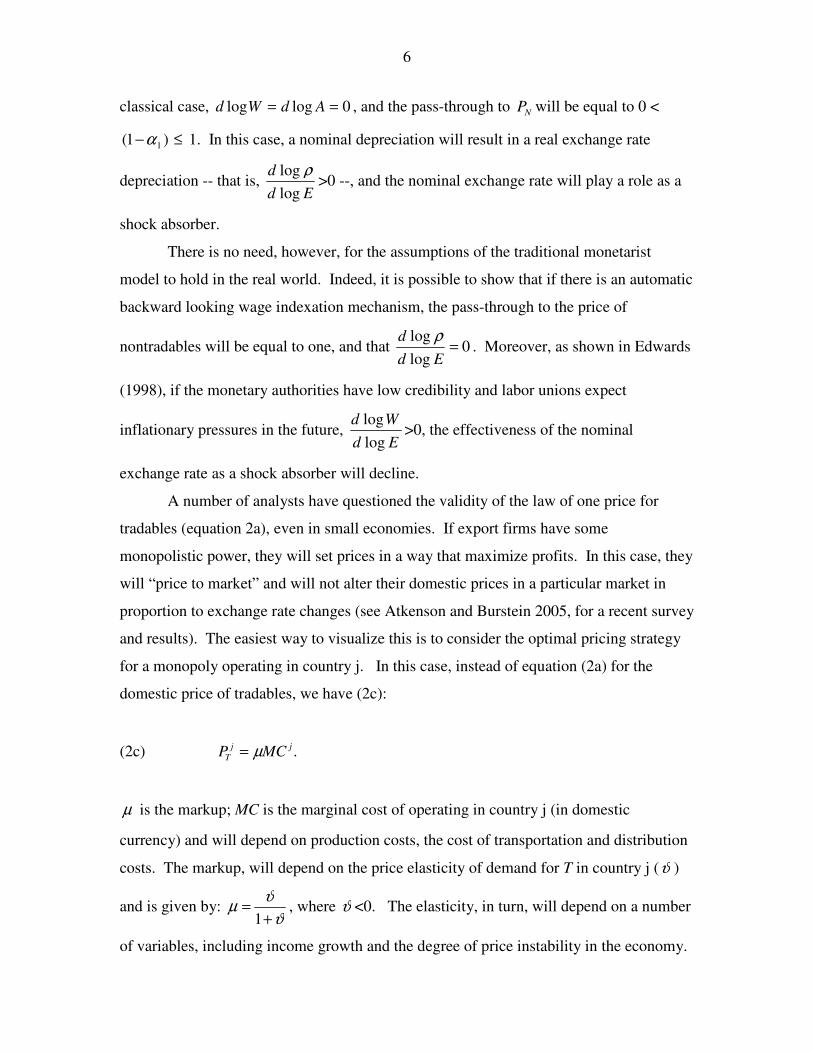
for a monopoly operating in country j. In this case, instead of equation (2a) for the

domestic price of tradables, we have (2c):

(2c) .jjT MCP µ=

µ is the markup; MC is the marginal cost of operating in country j (in domestic

currency) and will depend on production costs, the cost of transportation and distribution

costs. The markup, will depend on the price elasticity of demand for T in country j (ϑ )

and is given by: ϑ

ϑµ+

=1

, where ϑ <0. The elasticity, in turn, will depend on a number

of variables, including income growth and the degree of price instability in the economy.

7

It is clear from (2c) that under most circumstances a change in the nominal exchange rate

will not be translated into a one-to-one change in the domestic price of tradables. This is

for two reasons: first, MC needs not remain constant when E changes. And second, the

mark-up will not remain unchanged when the exchange rate depreciates; indeed, it is

likely to decline.9 This means that the magnitude of the pass-through from exchange rate

to the price of tradables is likely to be smaller than one. In the extreme case when the

pass-through into importable goods is zero we say that the market is characterized by

“local currency pricing.”

Although the framework developed here could be made more complex – by

assuming that nontradables use tradable inputs, for example --, the main points would

still be valid. In particular, once the role of the real exchange rate is explicitly introduced

into the analysis, it is important to distinguish between two notions of exchange rate pass-

through: pass-through into nontradables, and pass-through into tradables. In this

context, and from a policy perspective, a desirable situation is one where pass-through

coefficients for tradables and nontradables are low and different, with the pass through

for tradable goods being higher than that for nontradables.

In this section I use data from seven countries that have adopted inflation

targeting to investigate whether the magnitude of the pass-through has been affected by

the adoption of this monetary policy; see Table 1 for a list of countries and the date when

IT was enacted. One of the main objectives of this analysis is to investigate whether the

adoption of IT has affected the effectiveness of nominal exchange rates as shock

absorbers. As pointed out above, this would be the case if the pass-through from

exchange rates to nontradable prices has declined and/or the pass-through to tradables

goods has increased (or, at least, has not declined).

II.2 Empirical Model

An empirical analysis of the pass-through that focuses on inflation and the real

exchange rate would consider the way in which changes in nominal exchange rates affect

the domestic prices of nontradable and tradable goods. In most countries, however, there

are important data limitations; in particular, very few countries have data on nontradables

prices. Data limitations are more severe in emerging countries, where long series of

9 This is the case under many forms of the demand curve.

8

domestic prices of importables are rarely available.10 For this reason, in the empirical

analysis that follows I have used the CPI index as a proxy for the domestic price of

nontradables ( NP ) and the PPI as a proxy for the domestic price of tradables ( TP ). This

means that I am using the ratio ��

���

�

CPIPPI

as a proxy for the real exchange rate in equation

(1). As it turns out, and as is illustrated in Figure 1 for the case of Chile, in many

countries this is a fairly good proxy for the (effective) real exchange rate.

Most empirical studies on pass-through have estimated variants of the following

equation (Campa and Goldberg 2002; Gagnon and Ihrig 2004):

(4) tttititt PPxEP ωβββββ +∆+∆++∆+=∆ −� 14*

3210 loglogloglog .

Where tP is a price index -- either of importables, tradables or nontradables --, E is the

nominal exchange rate, *P is the an index of foreign prices, the sβ are parameters to be

estimated, the sx j are other controls expected to capture changes in the markup, and jω

is an error term with standard characteristics. The short run pass-through is given by 1β

and the long term pass-through is )1( 4

1

ββ−

.11 Many analysts have imposed the

constraint 31 ββ = . In this paper, however, I consider the more general case, and I allow

for different coefficients for the nominal exchange rate and international prices.12

From an empirical point of view the question of interest is whether the

coefficients 1β and 4β have experienced a structural change at (approximately) the time

of the adoption of inflation targeting. I investigate this by adding two interactive terms to

equation (4). The equation that I actually estimated is:

10 In the IFS, unit import prices for industrialized countries are expressed in domestic currency. However, for most emerging countries they are expressed in US dollars. 11 Campa and Goldberg (2002) used the sum of four lagged coefficients of the change in the exchange rate to compute the long run pass-through. The distributed-lags approach used by Campa and Goldberg is also followed by most other authors. 12 Some studies, such as Gagnon and Ihring (2004), have analyzed how different monetary regimes have affected the extent of pass-through.

9

(4a)

tt

ttiitjt

DITP

DITEPPxEP

ωβββββββ

+×∆+

×∆+∆+∆++∆+=∆

−

−�16

514*

3210

log

logloglogloglog

Where DIT is a dummy variable that takes the value of one at (approximately) the time IT

is adopted, and zero otherwise. The short term pass-through in the post-IT period is

51 ββ + . Notice that, in contrast with other studies, in (4a) I allow the coefficient of

lagged Plog∆ during the post-IT period to be different from the pre-IT coefficient. This

is important for two reasons: first, it allows investigating whether, as argued by Taylor

(2000), a more inflationary-focused policy reduces inflationary inertia. Second, it

provides an alternative channel through which the long run pass-through may decline.

Indeed, since the long run pass-through in the post-IT period is ���

����

�

+−+

)(1 64

51

ββββ

, it may

be lower than the pre-IT coefficient either because 5β or 6β are significantly negative in

equation (4a).

In spite of its simplicity, the estimation of equations of the type of (4a) presents

several challenges. The most important has to do with potential endogeneity problems.

Indeed, it is possible that Elog∆ in equation (4a) is not exogenous, and is correlated with

the error term. In principle, there are several ways to deal with this issue; none of them,

however, is particular satisfactory from a practical point of view. First, equation (4a)

could be estimated using simultaneous equations methods, such as two stage least squares

or generalized method of moments. The problem is that, as is well known, in the vast

majority of countries with floating exchange rates it is very difficult to find good

instruments for Elog∆ ; most exogenous variables are not highly correlated with changes

in the nominal exchange rate.13 Second, structural VARs could be estimated. However,

identification conditions require making assumptions about the timing of the effects of

exchange rate on prices that are not particularly convincing. For these reasons, most

recent studies on pass through, including Campa and Goldberg (2002) and Gagnon and

Ihrig (2004) have relied on least squares methods. An additional challenge in the

13 This difficulty was first pointed out by Meese and Rogoff (1983).

10

estimation of (4a) is that many countries don’t have data on the (possible) determinant of

the markup, or additional controls x in equation (4a).

II.3 Data and Empirical Results

In the estimation of equation (4a) I use quarterly data for the period 1985-2005 for

seven countries – two advanced and five emerging – that have adopted inflation targeting

at some point during the last 15 years (see Table 1).14 Some of these countries – Chile is

the premier example – adopted IT in an evolutionary fashion. For this reason, in Table 1

I provide two dates for the adoption of IT in Chile: 1991, when an inflation target range

was first announced, and 1994 when a specific inflation rate was adopted as a target .15

Unless I indicate otherwise, the results reported in this section were obtained when the

mid 1994 date was used as the launching date of IT in Chile. When the alternative

1991date was used, the results obtained were similar.

For each country I estimated two equations: one for the rate of change of the CPI

(which, as mentioned, is a proxy for nontradables inflation), and one for the rate of

change of the PPI (a proxy for domestic tradables inflation). All data are expressed as

quarterly percentage changes. The exchange rate is the effective (multilateral) exchange

rate, defined as the domestic price of a basket of currencies. Thus, an increase in E is a

(multilateral) nominal depreciation.16 To the extent that it takes some time for a new

policy regime to be understood by the public, we would expect that the structural change

in the pass-through coefficients would not be instantaneous; it is likely to take place some

quarters after the new policy is adopted. In the estimation of (4a) I considered alternative

lags for DIT; most of the results reported in Table 2 are for four lags. The rate of change

of the US producer price index was used as a proxy for world inflation. In the basic

results reported in Table 2, I follow Gagnon and Ihrig (2004) and I do not include

additional controls x . See, however, the discussion below.

Since, for each country, the errors in the CPI and PPI equations are likely to be

correlated, I estimated the two equations for each country simultaneously, using Zellner’s

14 In some countries the time period was slightly shorter. 15 Alternatively one could use March 2000, when a Monetary Report was first published, as the relevant date. 16 For the majority of countries the multilateral effective exchange rate was taken from the IFS. For those countries for which the IFS does not provide the effective rate, I constructed a multilateral exchange rate index.

11

seemingly unrelated regressions (SURE) procedure.17 The results obtained are presented

in Table 2. In Table 3, on the other hand, I present a summary of the pass-through

coefficients in the pre-inflation targeting and post-inflation targeting periods. The main

results obtained may be summarized as follows:

• In all countries the pre-IT short term pass-through coefficient in the CPI

equation is positive. It is significantly so in six out of the seven countries;

the only exception is Canada whose coefficient is positive but not

significant.18 However, the estimated coefficients show a significant

degree of variability across countries. The short-run, pre-IT pass-through

coefficient into nontradable prices (CPI) ranges from a low of 0.020 in

Korea, to a very high 0.719 in Brazil. A simple inspection at these

estimates suggests that, historically, the CPI pass-through coefficient has

been much higher in countries with a tradition of high and chronic

inflation (e.g. Brazil), than in countries with traditional price stability (e.g.

Korea).

• Also, in six out of the seven countries the short term pass-through

coefficient in the PPI (or tradables) equation is significantly positive.

There is also a significant variability across countries.

• For the pre-IT period, the point estimate of the short term pass-through

coefficient is higher for tradables (PPI) than for nontradables (CPI) in all

countries.

• In most countries, and during the pre-IT period, the long-run point

estimate for the PPI pass-through is higher than for the CPI pass-through.

• In every case, the estimated coefficient of ( )DITEd ×log is negative. It

is significantly so in the majority of cases. This indicates that the short

run pass-through has declined in every country in the sample in the post-

IT period. Moreover, in most cases the decline has been larger in the CPI

(or nontradable) equation than in the PPI equation, indicating that there

17 In all equations I also included a time trend and, in the case of Brazil, two dummy variables for the 1989 and 1999 currency crises. 18 In the analysis that follows I consider as “significant” coefficients with a p-value of 20% or lower. In the majority of cases, however, the p-values are smaller than 5%.

12

has been an increase in the short run effectiveness of the nominal

exchange rate.

• The decline in the short run CPI pass-through in the post-IT period has

been particularly dramatic in the case of Brazil, where the short run

coefficient declined from 0.719 to 0.056. Other cases of major reduction

in the pass-through coefficient are Chile, Israel and Mexico. At the other

extreme, the change in the degree of CPI (or nontradable) pass-through in

Korea is not statistically significant; in this country the CPI pass-through

was already very low (0.020).

• The estimates in Table 2 show that in the pre-IT period inflation was

characterized by a considerable degree of inertia in most countries –

measured by the coefficient of lagged Plog∆ . Notice, however, that in

most cases, inertia was higher for CPI (or nontradable) inflation than for

PPI (or tradables) inflation.

• The estimated coefficients of ( )DITP ×∆ −1log are negative in the vast

majority of the countries – the exceptions are Brazil for both definitions of

inflation, and Israel for CPI. The estimated coefficient for

( )DITP ×∆ −1log is negative and statistically significant for Australia

(CPI), Canada (CPI), and Mexico (CPI and PPI), indicating that in those

countries inflationary inertia has significantly declined in the post-IT

period.

• The post-IT long run pass-through depends both on the behavior of

( )DITP ×∆ −1log and ( )DITE ×log . As Table 3 shows, for the majority

of countries in the sample the long run pass through coefficient has

declined in the post-IT period. This is the case both for the CPI (or

nontradable) and for the PPI (or tradable) pass-through coefficients.

An interesting question is whether the differences in the pass-through coefficients

for the CPI (nontradable) and PPI (tradable) equations reported in Tables 2 and 3 are

statistically significant. In order to address this issue I computed Wald 2χ statistics to

13

test for cross equation restrictions. The results obtained are reported in Table 4 (p-values

in parentheses). The test statistics are 2χ with one degree of freedom, and the null

hypothesis is that the pass-through coefficients in the CPI and PPI equations are equal in

each country. As may be seen, the null hypothesis is rejected at conventional levels in 4

of the seven countries.19 A particularly interesting case is that of Brazil, where the null

hypothesis was rejected both in the short and long run in the pre-IT period, and is only

rejected in the short run in the post-IT period. As a way of gaining further insights, I also

tested the joint hypothesis that the short and long run pass-through coefficients were

equal in both the pre and post-IT periods. The results – available on request – indicate

that the null hypothesis is rejected for Brazil, Canada and Mexico.

In the estimates reported in Table 2 I included a small number of controls. In

order to check for the robustness of the results – and, in particular, to check for possible

omitted variables bias – I also estimated equation (4a) including the following controls:

(a) deviations of GDP from a stochastic trend, lagged one or two periods (In some

regressions this variable was also interacted with the nominal depreciation); (b)

deviations of US GSP, lagged one and two periods; (c) the change in the degree of

volatility of inflation, lagged one or two periods. (In some regressions this variable was

also interacted with the nominal depreciation); and (d) a time trend. The results obtained

are very similar to those presented in Table 2 and confirm that in most countries there

have been breakpoints in the short run pass-through, the degree of inertia and the long

ruin pass-through coefficient.20

II.4 Further Results and Comments on Chile’s Experience

Chile has been a pioneering in the implementation of inflation targeting in

emerging countries. What makes this case particularly interesting is that for decades

Chile had a high and chronic inflation. Starting in the 1940s inflation increased

significantly and became a major political and economic problem; until the 1990s

repeated efforts to quell it proved to be unsuccessful (Meller 1996). In his celebrated

work on inflationary inertia, Pazos (1972) referred to Chile as the premier case of an

economy where inflation tended to perpetuate itself. Numerous scholars have analyzed

19 Although in most of them the rejection is not across all time-runs and time periods. 20 Results available on request.

14

the historical behavior of inflation in Chile, and have concluded that fiscal largesse, low

Central Bank credibility, and widespread indexation practices (both for wages and the

nominal exchange rate) were behind Chile’s historical high rates of inflation. In the

1990’s, however, there were important changes in Chile’s monetary policy: the Central

bank was granted independence and it formally adopted an inflation targeting approach

(Corbo 1998, Schmidt-Hebbel and Tapia (2002), and Morandé (2002)). Since then

inflation has declined significantly. During the last few years it has not been significantly

different from world inflation.

The results presented in Tables 2 and 3 of this paper tend to confirm this story:

after the adoption of inflation targeting in the early 1990s Chile experienced a decline in

the degree of pass-through, both in the case of CPI inflation as well as PPI inflation (See-

also De Gregorio and Tokman, 2004). In this section I provide additional results on

Chile’s case that provide further light on the relation between inflation and exchange

rates. In Table 5 I present new estimates for equation (4a) for CPI (or nontradable)

inflation and CPI (or tradable) inflation using three stages least squares, which deals with

the potential endogeneity of exchange rate changes.21 As may be seen, although the point

estimates are somewhat different, the overall results tend to confirm the conclusions

reached above. Generally speaking, the 3SLS estimations show that the degree of both

CPI and PPI pass-through has declined in the post-IT period. Interestingly, and in

contrast with the cases of Australia, Canada and Mexico, there is no evidence of a decline

of the degree of inflationary inertia in Chile in the post-IT period. Moreover, in Chile the

level of inertia is similar for CPI and PPI inflation. From a comparative perspective,

however, inflationary inertia in Chile is not higher than in countries with a long tradition

of price stability, such as Australia and Canada (See Table 2).

III. Inflation Targeting and Exchange Rate Volatility: Some Empirical Tests

As a number of authors have pointed out, a floating exchange rate system is a

requirement for a well functioning inflation targeting regime (Mishkin and Savastano

21 The following instruments were used: lagged first-difference in the US CPI, commodity price index, and first-difference of the US PPI.

15

2001).22 The reason for this is that in a world of capital mobility, independent monetary

policy cannot coexist with a pegged exchange rate regime – this is the so-called

“Impossibility of the Holy Trinity.” This connection between inflation targeting and

floating exchange rates has led some analysts to argue that one of the costs of IT is the

increase in exchange rate volatility. In a recent paper, De Gregorio, Tokman and Valdés

(2005) discuss this issue in the Chilean context, and show that in Chile (nominal)

exchange rate volatility has not been higher than in other countries with floating

exchange rates.

The way in which the adoption of IT affects exchange rate volatility is an

important policy issue. Yet, it is one that has not been dealt with appropriately in recent

debates. Indeed, many analysts have compared exchange rate volatility under IT with

volatility under a pegged or administered exchange rate regime. This is not an adequate

comparison. From a policy evaluation perspective it is important to separate the issue of

the selection of the exchange rate regime with the adoption of IT. The correct question is

whether the adoption of IT increases exchange rate volatility, controlling for the

exchange rate regime. Moreover, most volatility analyses have been based on

comparisons of unconditional volatility measures across countries, or across time for the

same country.

There are several possible ways of addressing these issues. First, one can analyze

whether the adoption of IT affects conditional exchange rate volatility in countries that

have had a floating exchange rate for a prolonged period of time, such as Australia and

Canada. Second, regressions that control for the exchange rate regime can be estimated.

In this section I use both of these approaches and monthly data to analyze this issue. The

analysis focuses on the seven countries in Table 1. From a conceptual perspective, once

one conditions for the exchange rate regime, it is possible to determine whether IT, by

itself, results in an increase in exchange rate volatility. For example, in the cases of

Australia and Canada – two countries with a long tradition with floating rates -- a

comparison of conditional volatility before and after the implementation of IT will

provide information on the effects of the new policy regime on exchange rate behavior.

22 There is no need, however, for the authorities to abstain completely from intervention in the foreign exchange market. See the discussion in Section IV of this paper.

16

III.1 The Data and the Empirical Model

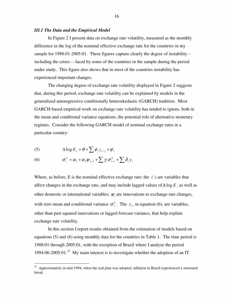
In Figure 2 I present data on exchange rate volatility, measured as the monthly

difference in the log of the nominal effective exchange rate for the countries in my

sample for 1988:01-2005:01. These figures capture clearly the degree of instability –

including the crises -- faced by some of the countries in the sample during the period

under study. This figure also shows that in most of the countries instability has

experienced important changes.

The changing degree of exchange rate volatility displayed in Figure 2 suggests

that, during this period, exchange rate volatility can be explained by models in the

generalized autoregressive conditionally heteroskedastic (GARCH) tradition. Most

GARCH-based empirical work on exchange rate volatility has tended to ignore, both in

the mean and conditional variance equations, the potential role of alternative monetary

regimes. Consider the following GARCH model of nominal exchange rates in a

particular country:

(5) � ++=∆ − tjtjt zE ψφθlog

(6) � �+++= −− iiititt yδσγψαασ 2121

2

Where, as before, E is the nominal effective exchange rate; the sz' are variables that

affect changes in the exchange rate, and may include lagged values of Elog∆ , as well as

other domestic or international variables; tψ are innovations to exchange rate changes,

with zero mean and conditional variance 2tσ . The ty , in equation (6), are variables,

other than past squared innovations or lagged forecast variance, that help explain

exchange rate volatility.

In this section I report results obtained from the estimation of models based on

equations (5) and (6) using monthly data for the countries in Table 1. The time period is

1988:01 through 2005:01, with the exception of Brazil where I analyze the period

1994:06-2005:01.23 My main interest is to investigate whether the adoption of an IT

23 Approximately in mid-1994, when the real plan was adopted, inflation in Brazil experienced a structural break.

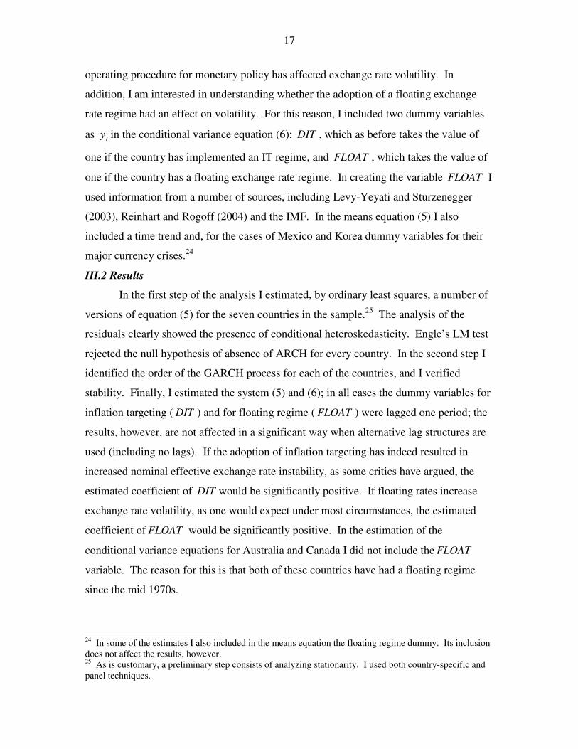
17

operating procedure for monetary policy has affected exchange rate volatility. In

addition, I am interested in understanding whether the adoption of a floating exchange

rate regime had an effect on volatility. For this reason, I included two dummy variables

as ty in the conditional variance equation (6): DIT , which as before takes the value of

one if the country has implemented an IT regime, and FLOAT , which takes the value of

one if the country has a floating exchange rate regime. In creating the variable FLOAT I

used information from a number of sources, including Levy-Yeyati and Sturzenegger

(2003), Reinhart and Rogoff (2004) and the IMF. In the means equation (5) I also

included a time trend and, for the cases of Mexico and Korea dummy variables for their

major currency crises.24

III.2 Results

In the first step of the analysis I estimated, by ordinary least squares, a number of

versions of equation (5) for the seven countries in the sample.25 The analysis of the

residuals clearly showed the presence of conditional heteroskedasticity. Engle’s LM test

rejected the null hypothesis of absence of ARCH for every country. In the second step I

identified the order of the GARCH process for each of the countries, and I verified

stability. Finally, I estimated the system (5) and (6); in all cases the dummy variables for

inflation targeting ( DIT ) and for floating regime ( FLOAT ) were lagged one period; the

results, however, are not affected in a significant way when alternative lag structures are

used (including no lags). If the adoption of inflation targeting has indeed resulted in

increased nominal effective exchange rate instability, as some critics have argued, the

estimated coefficient of DIT would be significantly positive. If floating rates increase

exchange rate volatility, as one would expect under most circumstances, the estimated

coefficient of FLOAT would be significantly positive. In the estimation of the

conditional variance equations for Australia and Canada I did not include the FLOAT

variable. The reason for this is that both of these countries have had a floating regime

since the mid 1970s.

24 In some of the estimates I also included in the means equation the floating regime dummy. Its inclusion does not affect the results, however. 25 As is customary, a preliminary step consists of analyzing stationarity. I used both country-specific and panel techniques.

18

The results obtained are in Table 6. I have only reported the order of the GARCH

process, and the estimated coefficients of DIT and FLOAT . The main results may be

summarized as follows:

• The estimated coefficient of the inflation targeting dummy DIT is positive

and very small in three of the countries – Australia, Canada, and Korea.

However, in none of these cases it is significantly different from zero.

This indicates that (at least in this sample) there is no evidence that the

adoption of IT increases nominal multilateral exchange rate volatility.

• The estimated coefficient of the inflation targeting dummy DIT is

significantly negative in three of the countries in the sample – Brazil,

Chile (for both equations), and Israel –, and negative (but not significant)

in Mexico. In the case of Chile, the degree of significance of DIT is

higher (in absolute terms) when 1994 is considered as the beginning of the

IT period. Interestingly, when the FLOAT variable is excluded, the

coefficient of DIT becomes positive (but insignificant) in the conditional

variance equations for Chile and Brazil. These results suggest that, after

controlling for the exchange rate regime, the adoption of IT has tended to

reduce conditional volatility in some countries. The most likely reason for

this is that IT is a transparent and predictable monetary framework that

tends to reduce unexpected shocks or “news.”

• The estimated coefficient of the FLOAT variable is positive in the five

equations where it was included. Moreover, it is significantly positive in

three of the five equations – for Brazil, Chile, and Israel.

The results reported in Table 6 are for standard GARCH models. In this setting

the nominal exchange rate reacts in the same way to positive and negative shocks.

However, as a number of authors have argued, it is possible that the nominal exchange

rate reacts in an asymmetric fashion to positive and negative shocks. In order to analyze

whether this possibility would affect the main results discussed above I estimated a series

of TGARCH and EGARCH models for the seven countries in the sample. Although

there is some evidence of asymmetric responses, the main conclusions on the coefficients

19

of DIT and FLOAT discussed above still hold: there is no evidence that, once one

controls for exchange rate regime, the volatility of nominal (multilateral) exchange rates

increased with the adoption of IT.

The results presented above are for nominal multilateral exchange rates. An

interesting question is whether the adoption of IT has affected real effective exchange

rate volatility. In order to analyze this issue I estimated equations of the type of (5) and

(6) for the four countries with data on real effective exchange rates at the monthly

frequency – Australia, Canada, Chile and Israel. The results obtained are presented in

Table 7. As may be seen, they tend to confirm those obtained for nominal multilateral

exchange rate volatility. There is no evidence that the adoption of IT has increased real

effective exchange rate volatility. In fact, there is some evidence that the opposite has

happened in Chile and Israel; in both of these countries the coefficient of DIT is negative,

with a Z-statistic in excess (in absolute terms) of 1.2. As in Table 6, these estimates

suggest that the adoption of a floating regime increased RER volatility: the estimated

coefficients of the FLOAT dummy are significantly positive.

III.3 Extensions for the Case of Chile

The results reported above span a period where most – but not all – of the

countries in the sample experienced important changes in their exchange rate regime.

Chile is a case in point.26 During this period the country went from having an exchange

rate band of varying width to having a flexible exchange rate. It may be argued, thus,

that the extent of exchange rate volatility during the band period was limited by the

existence of the band itself, even if the actual exchange rate never hit the bands. If this is

the case, the results for the emerging countries – but not for Australia or Canada – in

Table 6 maybe misleading. In order to deal with this issue in this section I use data on

Chile’s shadow nominal exchange rate – or exchange rate that would have prevailed in

the absence of the bands – to analyze exchange rate volatility in the period 1991-2004.

The data on the shadow exchange rate were taken from Edwards and Rigobon (2005).

This shadow rate was computed using an iterative procedure based on the behavior of the

actual rate, the bands and the fundamentals. Figure 3 presents the evolution of the

26 This also applies to Mexico and Israel. Mexico had a band until late 1994; Israel had a widening crawling band into the 2000s. Korea had a managed exchange rate until 1998; Brazil had a managed rate until 1999.

20

monthly change of the nominal observed and nominal shadow exchange rate for the

Chilean peso relative to the U.S. dollar

The estimation of the conditional variance equation for the shadow exchange rate

yielded the following results: the point estimate for the inflation targeting dummy

DIT was -2.36E-05, with a z-statistic of -0.406. The point estimate for the floating

exchange rate dummy FLOAT was 0.00004, with a z-statistic of 1.62.27 These results,

then, confirm those reported in the preceding subsection. Even when a shadow exchange

rate is used, there is no evidence suggesting that the adoption of IT increased nominal

exchange rate volatility; there is, on the other hand, some evidence indicating that the

move from a band to a floating regime did have a small (positive effect) on volatility.

IV. Central Bank Policy and the Exchange Rate under an IT Policy Regime

Should inflation targeting central banks intervene in the foreign exchange market?

And if so, how should this intervention take place? Should it be sterilized intervention,

where the resulting changes in monetary aggregates are sterilized through operations

involving domestic securities? Or should it be non-sterilized intervention, where

monetary aggregates are affected?28 These are complex questions that have moved to the

center of the policy debate in many IT countries, especially in Latin America. In this

section I discuss the issue of whether IT central banks should explicitly consider the

exchange rate in their monetary rule.29 This question is related to a number of important

(and controversial) policy issues, including the costs of (real) exchange rate misalignment

and “fear of floating.”30

27 In this estimation the 1994DIT dummy was used. 28 Questions do not end here, however. Here are some additional ones: If intervention is sterilized, what type of domestic securities should be used in the sterilization? Should the purchases/sales of forex be done in the spot or in the forward market? 29 It is not my intention to provide a comprehensive survey on the topic of central bank intervention. The literature is voluminous country-specific, and continues to grow every day; interested readers are directed to, among others, Dominguez and Frankel (1993), Taylor (2004), Kearns and Rigobon (2005), Neely (2001), Sarno and Taylor (2001). For an excellent analysis of different central bank policies, including Chile’s case, see Tapia and Tokman (2004). 30 On fear of floating see Calvo and Reinhart (2002).

21

IV.2 The Issues

From a technical point of view the discussion of the relation between central bank

policy and the exchange rate may be framed in terms of the form of the Taylor rule in a

small open economy. Taylor himself has posed the problem as follows

“How should the instruments of monetary policy (the interest rate or a

monetary aggregate) react to the exchange rate?” (Taylor, 2001, p. 263.

Emphasis added)

In order to address this question more formally, consider the following equation:31

(7) 110 −+++= ttttt ehehgyfi π

Where ti is the short term interest rate used by the central bank as a policy tool, tπ is the

deviation of the rate of inflation from its target level – possibly zero --, ty is the deviation

of real GDP from potential real GDP (often called the output gap), and e t is the log of the

real exchange rate in year t.32 f and g are the traditional Taylor rule coefficients; 0h and

1h are the coefficients of the current and lagged log of the real exchange rates in the

expanded Taylor rule, and are the main interest of this discussion. If 010 == hh exchange rate developments should not be incorporated in the policy rule, and the Taylor

rule reverts to its traditional form.

It is conceivable, in principle, that in a small open economy the optimal monetary

policy rule – that is the policy that maximizes the authorities’ objective function – is one

where both 0h and 1h are different from zero. Interestingly, if 00 >h and 10 hh −= , then

the rule implies that monetary policy should react to changes in the (real) exchange rate.

Notice that the formulation in equation (7) does not imply, even when 0h and 1h are

different from zero, that the monetary authorities should defend a certain level of the

exchange rate. If the optimal policy calls for intervention – that is for 0h and 1h different

31 This is the precise equation presented by Taylor in his discussion on the subject. 32 In this formulation an increase in e denotes a real exchange rate appreciation.

22

than zero --, and if the monetary authorities do follow this policy, a casual observer may

conclude that the country in question is subject to “fear of floating.” This, however,

would be an incorrect inference, as the country in question would be practicing “optimal

flotation.”

In order to answer fully this question it is necessary to specify the policy maker’s

objective (or loss) function, and the model that best captures the functioning of the

economy. Most authors assume that the goal of policy makers is to minimize a loss

function that combines deviations of GDP (or GDP growth) from trend and deviations of

inflation from its target.33

(8) 22 )~()~( yyL tt −+−= λππ , and 0>λ .

In equation (8) π and y are the inflation target and potential output; )ˆ( yy t − is the output

gap. It is easy to show that in this case the only way in which the exchange rate could

play a role in the monetary policy rule would be one where changes in e (or, in some

models, changes in the nominal exchange rate) affect inflation and/or the output gap. To

the extent that the “pass-through” coefficient is different from zero, exchange rate

changes will affect actual inflation – that is, 0>∂∂

eπ

. If (some) changes in the real

exchange rate reflect situations of misalignment they will affect the output gap. Under

these circumstances, the optimal policy will be one that takes into account the way in

which exchange rate developments affect the two components of the loss function. What

is unclear, however, is whether the exchange rate should have an independent role in the

monetary policy rule (8). If the authorities have modeled the economy correctly – and in

doing so, have incorporated the effects of e on π and y -- there is no need to include an

exchange rate term in equation (8). This point has been made forcefully by De Gregorio,

Tokman and Valdés (2005) in their discussion of Chile’s case. If, however, there is a

lagged response of both inflation and output to exchange rate changes, the central bank

33 Medina and Valdés (2002) develop a model where the authorities also target the current account. They show that the optimal reaction function is significantly different from the traditional Taylor rules.

23

may want to preempt their effect by adjusting the policy stance when the exchange rate

change occurs, rather than when its effects on π and y are manifested.

Whether a pre-emptive strategy is preferred to one where the authorities actually

wait untilπ and y begin to reflect the actual effects of a change in e is, in the final

analysis, an empirical issue. Moreover, it is a country specific issue; the main

characteristics of a particular economy – including the dynamics of inflation, the size of

the pass-through coefficient, and of different elasticities – will determine the extent of

macroeconomic volatility – that is deviations of inflation and growth from targets and

trends – is lower when 0h and 1h are different from zero.

IV.2 A Selective Review of the Literature

Most analytical discussions on inflation targeting have implicitly assumed

that 010 == hh , without actually inquiring the way in which the incorporation of e into

the policy rule will be affect welfare and/or macroeconomic performance. In fact, things

go even further: most discussions on IT in the mainstream literature have tended to ignore

open economy issues. In the important book The Inflation Targeting Debate edited by

Ben Bernanke and Mike Woodford, the index has no entry for “devaluation” or “pass-

through”, and there is only one entry for “exchange rate.” This corresponds to the paper

by Jonas and Mishkin (2005) on IT in transition economies. Most of the other papers in

the volume – authored by influential economists such as Woodford, Bernanke, and Sims,

among others – do not include explicit discussions on exchange rate behavior when

dealing with monetary policy issues. There are, however, a few exceptions: in their

paper, Cecchetti and Kim (2005) have a section on an open economy, but do not ask

formally whether 0h and/or 1h should be equal to zero. In his contribution to the

Bernanke and Woodford volume, Mervyn King briefly notes that although the U.K.

experienced a sharp currency appreciation (in excess of 20%) this had not affected the

effectiveness of the IT-based policy. Caballero and Krishnamurthy (2005) develop a

model of an open economy where the exchange rate plays an important role during a

“sudden stop” episode. In their setting the exchange rate does play an important role in

determining optimal monetary policy.

24

The seminal book by Mike Woodford, Interest and Prices (2003), which provides

firm analytical underpinnings for interest rate-based monetary policy, does not deal

explicitly with exchange rates; the index has no entries for “exchange rate(s),”

“devaluation,” or “pass-through.” There is one entry for “open economy,” although no

open economy model is presented, and the discussions on optimal policy rule do not

consider the (potential) role of open economy variables. (To be fair, however, one could

interpret the discussion in section 2.1 of Chapter 7, on cost-push shocks, as including

shocks stemming from exchange rate depreciation.)

The pioneering book by Bernanke et al (1999) includes interesting discussions on

the role played by exchange rates in monetary policy implementation in a number of

countries. The discussion of the Canadian case – where a Monetary Conditions Index

(MCI) that includes the exchange rate has been used explicitly is particularly

interesting.34 However, the important chapter on “Design and Implementation,” (Chapter

3) does not discuss at the analytical level whether exchange rate considerations should be

explicitly incorporated into the policy rule in an inflation targeting setting. In the chapter

on Israel, Australia and Spain the authors discuss how Spain and Israel gradually relaxed

exchange rate bands when they adopted IT, and they explain that in both of these

countries the authorities decided “not to respond to short term exchange rate fluctuations”

when making monetary policy decisions (Bernanke et al, 1999, page 205).

Mishkin and Savastano (2001) provide one of the most complete discussions on

the issue. These authors convincingly argue that the discussion on macroeconomic

stability in Latin America is not related to the selection of the exchange rate regime. The

issue is one of creating an institutional framework for conducting monetary policy in a

credible way. According to them IT provides such a framework. Mishkin and Savastano

develop a model where optimality implies a Taylor rule of the following form:

(9) tttt ebybbi 32*

1 )( ++−+= πππ .

34 New Zealand also adopted a MCI in the late 1990s.

25

te is the log of the real exchange rate, expressed as deviations from its equilibrium value.

The authors make a very important point:

“[I]n Latin America exchange rate fluctuations are likely to have a bigger

effect on aggregate demand and aggregate supply (because the pass-

through may be larger)…indicates that the weight of the exchange rate in

the modified Taylor-rule, 3b , may be relatively large. However, this is in

no way inconsistent with inflation targeting) (Mishkin and Savastano,

2001, page 534).

Ball (1999), Obstfeld and Rogoff (1995) and Svensson (2000) have argued that

adding the exchange rate as an additional variable in equations of the type of (7) will

result in more stable macroeconomic outcomes. According to a simulation exercise

undertaken by Svensson (1999, 2000) the optimal values of the exchange rate coefficients

are 0h = -0.45 and 1h = 0.45. Ball (1999) analysis suggests that macroeconomic

instability will be reduced if 0h = -0.37 and 1h = 0.17. These results, however, are

model-specific and they will change for different parameterizations.

In a paper presented at a Central Bank of Chile conference, Taylor (2002)

reviewed 19 recent models developed to analyze inflation and monetary issues. Of these,

only 5 assumed that the exchange rate affected aggregate demand, and only six assumed

that exchange rate changes was a factor in the process of price determination. This

illustrates quite starkly the fact that many influential researchers continue to think in

terms of closed economy monetary models.

At the end of the road, whether 0h and 1h should indeed be different from zero is

a country-specific empirical question, that should be dealt with by analyzing country

specific evidence – both historical and based on simulation exercises. After much

reflecting on this subject I find it difficult to disagree with Taylor (2001) when he

expresses some skepticism on the general merits of adding the exchange rate into the

interest rate equation. This is for, at least, two reasons. First, and as pointed out earlier,

in properly specified models, the exchange rate already plays an indirect role through its

26

effect on tπ and ty ; second, adding the exchange rate (or any other asset price, for that

matter) into the Taylor rule is likely to add considerable volatility to monetary policy.

This conclusion is similar to that of Mishkin and Schmidt-Hebbel (2001) who provide an

extensive discussion on the subject. According to them, when implementing policy,

central banks should consider the effects of exchange rate fluctuations on inflation and

the output gap, but should not consider an independent role for .te According to them,

“targeting on an exchange rate is likely to worsen the performance of monetary policy.”

IV.3 What do IT Central Banks Actually Do?

The discussion presented above clearly indicates that the issue of whether

monetary policy should react to the exchange rate is not fully resolved. At the analytical

level the answer is likely to be country specific and will depend on the structural

characteristics of the country, and the authorities’ loss function.

The vast majority of central banks, however, do not openly recognize that they

explicitly take into account exchange rate developments when conducting monetary

policy. Indeed, if pressed, most IT central bankers would go as far a saying that since

exchange rate changes tend to affect inflation, they play a role on monetary policy.

However, they would be reluctant to acknowledge that the exchange rate plays a direct

role of its own in the monetary policy rule itself. That is, in terms of equation (7), the

vast majority of IT central bankers would say that in their policy rules: 010 == hh .

As every student of monetary policy knows, however, in most countries there are

divergences between what central banks say they do, and what central banks actually do.

In a recent paper, Mohanty and Klau (2005) estimated monetary policy reaction functions

(i.e. Taylor rules) for 13 emerging and transition economies, and found out that in eleven

of them the coefficient of real exchange rate was significant.35 This provides strong

indication that, contrary to what they state, most IT central banks do take central bank

developments into account when determining their monetary policy stance. In Table 8 I

35 Other authors that have estimated central bank reaction functions to analyze whether the exchange rate plays a role include Hamermann (2005).

27

present a list of the countries with the estimated short and long term coefficients in the

estimated Taylor-rule reaction functions.36

The case of Chile is particularly interesting. According to Mohanty and Klau

(2005) base estimates, Chile’s Taylor rule may be expressed as follows (t-statistics in

parentheses):

11 32.035.035.032.097.032.0 −− +∆−∆+++= tttttt ixrxryi π , (0.25) (4.87) (1.25) (2.78) (-2.40) (4.03)

where xr∆ is the change in the real exchange rate. The data are quarterly and the time

period covered is from 1992 to 2002. What is particularly interesting about the Chilean

case is that the effect of (real) exchange rate changes on Central Bank policy appears to

last only one quarter. Indeed the sum of the coefficients for txr∆ and 1−∆ txr add up to zero.

As the results summarized in Table 8 show, there is a wide range of values for

both the short run and long run estimated coefficients of the real exchange rate in these

Taylor rule reaction functions. (The short run is defined as the sum of the coefficients of

txr∆ and 1−∆ txr . The long run is the sum of these two coefficients divided by one minus

the coefficient of .1−ty ). Short run coefficients, for example, go from a relatively high

0.79 for Mexico, all the way to zero for Chile; long run coefficients show an even larger

dispersion.37 In order to understand why in some countries monetary policy appears to

have been more susceptible to exchange rate changes than I others, I estimated a number

of cross country regressions. The dependent variable is the short run exchange rate

coefficient reported in Table 8. The following controls were used: (a) average inflation

1990-1995; (b) standard deviation of quarterly inflation 1990-1995; (c) standard

deviation of the real exchange rate 1990-1995; (d) degree of openness of the economy

measured as imports plus exports over GDP; (e) length of period for which the country

has had floating rates; and (f) number of years since IT was adopted. The results

obtained for these six univariate regressions are presented in Table 9. Since I only have 36 The coefficients in Table 7 have positive signs, since in this paper I have considered that a higher exchange rate represents depreciation. In the Mohanty and Klau paper higher rate represents appreciation, and the coefficients are negative. 37 In the case of long run coefficients, most of the very high values are the result of a very low estimate for the lagged interest rate. This may be biasing the long run estimates.

28

13 observations no attempt was made at running a multivariate regression with all the

regressors. In spite of the fact that the sample is extremely small, the results reported in

Table 9 are interesting and suggestive. Countries with history of higher inflation seem to

have a higher coefficient for xr∆ in their Taylor rules. Also, countries that have

historically had a more volatile (real) exchange rate seem to attach a higher coefficient to

the exchange rate in their monetary rule. When both variables are included in a bi-variate

regression their coefficient are still positive and continue to have a relatively high level of

significance.

V. Concluding Remarks

The exchange rate is one of the most important macroeconomic variables in the

emerging and transition countries. It affects inflation, exports, imports and economic

activity. For decades the vast majority of emerging countries had rigid exchange rate

regimes – either pegs (adjustable or hard) or managed. This, however, has changed

during the last few years, when an increasingly large number of countries have adopted

flexible exchange rate regimes. This move away from exchange rate rigidity has tended

to take place at the same time as many countries have embraced inflation targeting as a

way of conducting monetary policy. The conjunction of IT and flexible rates has brought

to the center of the discussion a host of new policy issues, including issues related to the

role of the exchange rate in monetary policy, volatility and the relationship between

exchange rate changes and inflation.

In this paper I have addressed three of this issues: (a) the relationship between the

pass-through and the effectiveness of nominal exchange rates in IT regimes; (b) the

effects of IT on exchange rate volatility; and (c) the role (or potential role) of exchange

rate changes on the monetary rule in IT countries. The main findings from this analysis

may be summarized as follows: (1) Countries that have adopted IT have experienced a

declined in the pas-through from exchange rate changes to inflation. In many of the

countries in the sample this decline in the pass-through has been different from CPI

inflation than for PPI inflation. There is no evidence, however, of changes in the degree

of effectiveness of the nominal exchange rate as a shock absorber. (2) The adoption of

IT monetary policy procedures has not resulted in an increase in (nominal or real)

29

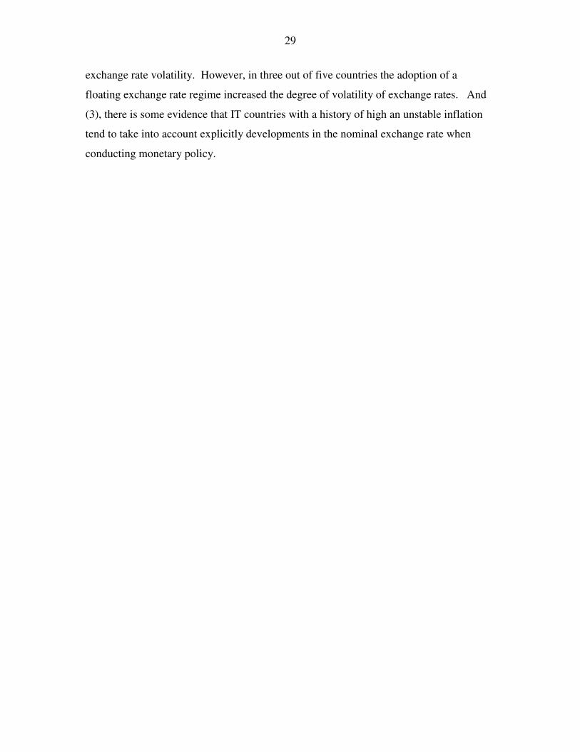
exchange rate volatility. However, in three out of five countries the adoption of a

floating exchange rate regime increased the degree of volatility of exchange rates. And

(3), there is some evidence that IT countries with a history of high an unstable inflation

tend to take into account explicitly developments in the nominal exchange rate when

conducting monetary policy.

30

-.2

-.1

.0

.1

.2

.3

4.5

4.6

4.7

4.8

4.9

5.0

88 90 92 94 96 98 00 02 04

Producer Price and Consumer Price RatioEffective Real Exchange Rate

Figure 1: Chile, Alternative Measures of Real Exchange Rate

31

-.06

-.04

-.02

.00

.02

.04

.06

88 90 92 94 96 98 00 02 04

Australia

-.2

-.1

.0

.1

.2

.3

.4

.5

88 90 92 94 96 98 00 02 04

Brazil

-.05

-.04

-.03

-.02

-.01

.00

.01

.02

.03

.04

88 90 92 94 96 98 00 02 04

Canada

-.08

-.06

-.04

-.02

.00

.02

.04

.06

.08

88 90 92 94 96 98 00 02 04

Chile

-.04

.00

.04

.08

.12

88 90 92 94 96 98 00 02 04

Israel

-.2

-.1

.0

.1

.2

.3

.4

88 90 92 94 96 98 00 02 04

Korea

-.1

.0

.1

.2

.3

.4

88 90 92 94 96 98 00 02 04

Mexico

Figure 2: Monthly Nominal Effective Exchange Rate Volatility

32

-.08

-.06

-.04

-.02

.00

.02

.04

.06

.08

-.08

-.06

-.04

-.02

.00

.02

.04

.06

.08

1992 1994 1996 1998 2000 2002 2004

Shadow Nominal Exchange RateObserved Nominal Exchange Rate

Figure 3: Monthly Changes in Observed and Shadow Nominal Exchange Rate

33

Table 1

Inflation Targeting: Selected Countries

Country

Inflation Targeting:

Starting Date

Australia Apr-93

Brazil Jun-99

Canada Feb-91

Chile June-91, June-94

Israel Dec-91

Korea Jan-98

Mexico Jan-99

Source: Central Bank’s monetary policy reports and press releases;

Various Central Bank of Chile and IMF research papers.

34

Table 2

SUR Estimates: Exchange Pass-Through, Selected Countries

(Quarterly Data: 1986.1-2005.1)

Australia Brazil Canada Chile Israel Korea Mexico CPI PPI CPI PPI CPI PPI CPI PPI CPI PPI CPI PPI CPI PPI dlog E 0.054 0.070 0.719 0.759 0.039 0.085 0.137 0.207 0.624 0.627 0.020 0.055 0.191 0.246 (2.34) (1.31) (24.76) (22.30) (0.79) (0.79) (2.88) (2.08) (12.18) (5.95) (1.20) (2.10) (4.85) (5.98) dlog P* 0.184 0.481 0.117 0.404 0.128 0.070 0.028 0.254 0.017 0.202 0.006 0.137 0.184 0.313 (3.13) (3.65) (0.22) (1.66) (2.69) (0.66) (0.26) (1.10) (0.18) (1.54) (0.07) (0.88) (0.64) (1.29) dlog P-1 0.548 0.060 0.300 0.284 0.499 0.404 0.355 0.194 0.132 0.121 0.200 0.213 0.635 0.584 (4.09) (0.30) (10.38) (8.67) (3.99) (1.83) (3.43) (1.77) (2.84) (2.92) (2.07) (2.15) (10.49) (10.06) C 0.006 0.011 0.011 -0.013 0.004 0.003 0.003 0.016 0.024 0.018 0.013 0.003 0.026 0.021 (2.27) (2.51) (0.55) (0.54) (2.75) (1.24) (3.88) (1.66) (4.78) (4.33) (4.59) (0.94) (1.96) (1.79) DIT* dlog E -0.057 -0.054 -0.663 -0.524 -0.066 0.032 -0.132 -0.162 -0.427 -0.430 -0.031 -0.063 -0.176 -0.053 (1.55) (0.60) (4.95) (3.28) (1.20) (0.28) (2.27) (1.32) (5.23) (6.42) (0.43) (0.77) (1.05) (0.31) DIT* dlog P-1 -0.344 -0.011 0.866 0.379 -0.488 -0.054 -0.090 -0.120 0.120 -0.064 -0.097 -0.039 -0.454 -0.362 (1.76) (0.05) (1.51) (1.41) (2.77) (0.19) (0.79) (0.66) (0.92) (0.54) (0.43) (0.51) (2.02) (1.74) R2 0.467 0.234 0.974 0.964 0.349 0.220 0.667 0.169 0.866 0.880 0.210 0.110 0.793 0.790 Durbin-Watson.

2.11 2.17 2.39 2.41 2.14 2.06 2.13 1.74 2.46 2.10 2.15 2.32 2.31 2.37

Determinant residual covariance

- 4.85e-9 - 4.13e-6 - 1.49e-9 - 3.73e-8 - 2.98e-8 - 7.19e-9 - 5.23e-8

Time period 86.1-05.1

86.1-05.1

86.1-05.1

86.1-05.1

86.1-05.1

86.1-05.1

88.1-05.1

88.1-05.1

86.1-05.1

86.1-05.1

86.1-05.1

86.1-05.1

86.1-05.1

86.1-05.1

Absolute value of t-statistics are reported in parentheses E is nominal effective exchange rate, P* is the US producer price index, P-1 is one lag of domestic producer or consumer price index, and DIT is dummy for periods with inflation targeting.

35

Table 3

Short-Run and Long-Run Exchange Pass-Through, Selected Countries

(Quarterly Data: 1986.1-2005.1)

CPI Equations PPI Equations Short-run pass thorough Long-run pass thorough Short-run pass thorough Long-run pass thorough Pre-IT Post-IT Pre-IT Post-IT Pre-IT Post-IT Pre-IT Post-IT Australia 0.054 0.000 0.120 0.000 0.070 0.070 0.070 0.070 Brazil 0.719 0.056 1.027 -b 0.759 0.235 1.060 0.697 Canada 0.039a 0.000 0.078a 0.000 0.085a 0.085a 0.143a 0.143a Chile 0.137 0.005 0.212 0.008 0.207 0.045 0.257 0.056 Israel 0.624 0.197 0.718 -b 0.627 0.197 0.713 0.224 Korea 0.020 0.020 0.025 0.025 0.055 0.055 0.070 0.070 Mexico 0.191 0.015 0.523 0.018 0.246 0.246 0.591 0.316

Source: Author’s elaboration based on estimations reported in Table 2.

36

Table 4

Wald Tests for Cross Equation Restrictions

(�2 with one degree of freedom)

Short-Run Long-Run

Pre-IT Post-IT Pre-IT Post-IT

Australia 0.078 0.131 0.209 0.132

(0.78) (0.72) (0.65) (0.72)

Brazil 4.240* 3.966* 6.216* 0.543

(0.04) (0.04) (0.01) (0.46)

Canada 0.189 11.189** 0.085 8.219*

(0.66) (0.01) (0.77) (0.00)

Chile 0.721 0.251 0.140 0.214

(0.39) (0.61) (0.71) (0.64)

Israel 0.007 0.010 0.025 0.523

(0.93) (0.87) (0.87) (0.46)

Korea 3.466** 0.030 2.840** 0.051

(0.05) (0.91) (0.09) (0.92)

Mexico 23.523* 14.846* 3.824* 6.235*

(0.00) (0.00) (0.05) (0.01)

p-values in parenthesis * significant at 5% level ** significant at 10% level

37

Table 5

3SLS Estimates: Exchange Pass-Through, Chile

(Quarterly Data: 1988.1-2005.2)

CPI PPI dlog E-1 0.228 0.530 (1.55) (2.21) dlog P-1 0.375 0.281 (2.53) (1.62) dlog P* -0.035 0.213 (0.26) (0.72) C 0.024 0.000 (1.69) (0.00) DIT* dlog E -0.214 -0.446 (1.47) (2.00) DIT* dlog P-1 -0.105 -0.189 (0.62) (0.70) R2 0.647 0.056 Durbin-Watson 2.05 1.72 Time period 88.1-05.2 88.1-05.2 Determinant residual covariance 4.31e-0.8

Absolute value of t-statistics is reported in parentheses. E is nominal effective exchange rate, P* is the US producer price index, P-1 is one lag of domestic producer or consumer price index, and DIT is dummy for periods with inflation targeting. Instruments: lagged first-difference of the US CPI, commodity price index, and first-difference of the US PPI.

38

Table 6

GARCH Estimates: Inflation Targeting, Exchange Rate Regime,

and Nominal Exchange Rate Volatility, Selected Countries

(Monthly Data: 1988.1-2005.1)

Country DIT Float DW R2

Australia (1,1) 6.36e-06 - 1.96 0.10

(0.96) -

Brazil (2,2) -0.001 0.0008 1.97 0.25

(4.16) (2.55)

Canada (1,1) 6.73e-06 - 1.89 0.04

(0.66) -

Chile (1,1)a -7.48e-06 1.71e-07 1.96 0.18

(1.70) (3.57)

Chile (1,1)b -1.57e-05 2.54e-05 1.94 0.22

(4.20) (5.97)

Israel (1,1) -3.71e-04 3.94e-04 2.30 0.05

(5.44) (3.92)

Korea (1,0) 0.002 0.002 1.73 0.10

(0.94) (0.95)

Mexico (1,1) -3.67e-04 2.1e-04 2.50 0.14

(1.06) (0.63)

Absolute value of z-statistics are reported in parentheses. DIT is a dummy for periods with inflation targeting, and Float is a dummy for periods with floating exchange rate. a Inflation targeting assumed to start on June, 1991. b Inflation targeting assumed to start on June, 1994.

39

Table 7

GARCH Estimates: Inflation Targeting, Exchange Rate Regime, and Real Exchange

Rate Volatility, Selected Countries

(Monthly Data: 1988.1-2005.1)

Country Mean Equation GARCH DIT Float DW R2

Australia AR(2) (1,1) -1.77e-06 - 1.96 0.07

(0.52) -

Canada AR(3) (1,3) -3.67e-05 - 2.03 0.04

(1.11) -

Chilea AR(1) (2,2) -8.39e-06 2.50e-06 1.87 0.05

(1.27) (4.02)

Chileb AR(1) (2,2) -2.35e-05 4.66e-05 1.89 0.10

(2.57) (4.22)

Israel AR(1) (2,2) -3.47e-05 7.05e-05 1.89 0.09

(1.43) (1.75)

Absolute value of z-statistics is reported in parentheses. DIT is a dummy for periods with inflation targeting, and Float is a dummy for periods with floating exchange rate. a Inflation targeting assumed to start on June, 1991. b Inflation targeting assumed to start on June, 1994.

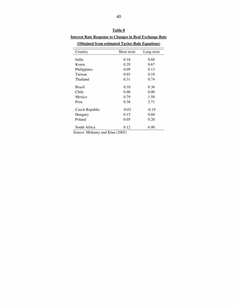
40

Table 8

Interest Rate Response to Changes in Real Exchange Rate

(Obtained from estimated Taylor-Rule Equations)

Country Short term Long term India 0.18 0.60 Korea 0.29 0.67 Philippines 0.09 0.13 Taiwan 0.03 0.18 Thailand 0.31 0.74 Brazil 0.10 0.36 Chile 0.00 0.00 Mexico 0.79 1.58 Peru 0.38 2.71 Czech Republic -0.03 -0.19 Hungary 0.15 0.60 Poland 0.05 0.20 South Africa 0.12 6.00

Source: Mohanty and Klau (2005)

41

Table 9

Exchange Rate Coefficient in Taylor-Rule Equations and Country Characteristics

(Ordinary Least Squares)

(1) (2) (3) (4) (5) (6)

Average Inflation 0.015

(1.74)***

St. Dev. Inflation 0.010

(0.71)

St. Dev. Real Exchange Rate 0.040

(1.78)***

Trade Openness -0.001

(0.64)

Length period with floating regime -0.000

(0.11)

Years since IT was adopted 0.005

(0.26)

Constant 0.037 0.140 -0.031 0.276 0.207 0.170

(0.35) (1.51) (0.23) (1.86) (1.17) (1.73)

Observations 13 13 13 13 13 13

R-squared 0.22 0.04 0.22 0.04 0.00 0.01

Absolute value of t statistics in parentheses *** significant at 10%; ** significant at 5%, * significant at 1%

42

REFERENCES Atkeson, Andrew and Ariel Burstein. 2005. "Trade Costs, Pricing to Market, and

International Relative Prices," mimeo, University of California at Los Angeles. Ball, Laurence. 1999. "Policy Rules for Open Economies," In J. Taylor (ed.): Monetary

Policy Rules, Chicago: University of Chicago Press. Bernanke, Ben S. 2004. "Central Bank Talk and Monetary Policy," speech before the

Japan Society, New York, New York, October 7. http://www.federalreserve.gov/boarddocs/speeches/2004/200410072/default.htm

Bernanke, Ben S. and Michael Woodford. 2005. The Inflation-Targeting Debate, NBER

Studies in Business Cycles, vol. 32. Chicago and London: University of Chicago Press.

Bernanke, Ben S., Laubach, Thomas, Mishkin, Frederic S., and Adam S. Posen. 1999.

Inflation Targeting: Lessons from the International Experience, Princeton, Princeton University Press.

Borensztein, Eduardo and , José De Gregorio. 1999. “Devaluation and Inflation after

Currency Crises,” Unpublished manuscript, Universidad de Chile, February. Caballero, Ricardo J. and Arvind Krishnamurthy. 2005. “Inflation Targeting and Sudden

Stops,” in Bernanke, Ben S. and Michael Woodford (eds.): The Inflation-Targeting Debate, NBER Studies in Business Cycles, vol. 32. Chicago and London: University of Chicago Press.

Calvo, Guillermo A. 1999. “Fixed vs. Flexible Exchange Rates” Fixed vs. Flexible

Exchange Rates: Preliminaries of a Turn-of-Millennium Rematch,” mimeo, University of Maryland.

Calvo, Guilermo A. and Carmen Reinhart, 2002, “Fear of Floating,” Quarterly Journal of

Economics, 117(2): 379-408. Campa, Jose Manuel and Linda S. Goldberg. 2002. “Exchange Rate Pass-Through into

Import Prices: A Macro or Micro Phenomenon?,” NBER WP 8934, May. Cecchetti Stephen G. and Junhan Kim. 2005. “Inflation Targeting, Price-Path Targeting,

and Output Variability,” in Bernanke, Ben S. and Michael Woodford (eds.): The Inflation-Targeting Debate, NBER Studies in Business Cycles, vol. 32. Chicago and London: University of Chicago Press.

Corbo, Vittorio. 1998. “Reaching One-Digit Inflation: The Chilean Experience,” Journal

of Applied Economics. 1(1): 123-63.

43

Corbo, Vittorio and Klaus Schmidt-Hebbel. 2003. “Inflation Targeting: The Latin American Experience,” in Gonzalez, Jose Antonio, et. al. (eds): Latin American Macroeconomic Reforms: The Second Stage. Chicago and London: University of Chicago Press: 19-71.

Della Paolera, Gerardo and Alan M. Taylor. 2003. New Economic History of Argentina,

Cambridge: Cambridge University Press, 2003 De Gregorio, José and Andrea Tokman. 2004. "Flexible Exchange Rate Regime and

Forex Interventions: The Chilean Case," Economic Policy Papers Nº 11, Central Bank of Chile, December.

De Gregorio, José, Tokman, Andrea, and Rodrigo Valdés. 2005. “Tipo de Cambio

Flexible con Metas de Inflación en Chile: Experiencia y Temas de Interés,”. Documento de Política Económica N°14. Banco Central de Chile. Agosto.

Diaz-Alejandro, Carlos F. 1970. Essays on the Economic History of the Argentine

Republic, New Haven, Conn.: Yale University Press. Domínguez, Kathryn and Jeffrey A. Frankel. 1993. “Does Foreign-Exchange Intervention

Matter?. The Portfolio Effect”. American Economic Review, 83(5): 1356-69. Edwards, Sebastian. 1998. “Two Crises: Inflationary Inertia and Credibility”, The

Economic Journal, 108 (May): 680-702. Edwards, Sebastian and Eduardo Levy Yeyati. 2005. “Flexible Exchange Rates as Shock

Absorbers,” European Economic Review, 49(8): 2079-2105 Edwards, Sebastian and Roberto Rigobon. 2005. “Capital Controls, Exchange Rate

Volatility and External Vulnerability,” NBER Working Paper No. 11434. Gagnon, Joseph E. and Jane Ihrig. 2004. “Monetary Policy and Exchange Rate Pass-

Through,” International Journal of Finance and Economics, 9(4): 315-338. Hammermann, Felix. 2005. “Do Exchange Rates Matter in Inflation Targeting Regimes?

Evidence from a VAR Analysis for Poland and Chile,” in Langhammer, R. J. and L. Vinhas de Souza, (Eds.): Monetary Policy and Macroeconomic Stabilization in Latin America.

Hochreiter, Eduard and Pierre L. Siklos, 2002. "Alternative Exchange-Rate Regimes: The

Options for Latin America," The North American Journal of Economics and Finance, 13(3): 195-211.

44

Jonas, Jiri and Frederic S. Mishkin. 2005. “Inflation Targeting in Transition Countries: Experience and Prospects,” in Bernanke, Ben S. and Michael Woodford (eds.): The Inflation-Targeting Debate, NBER Studies in Business Cycles, vol. 32. Chicago and London: University of Chicago Press.

Kearns, Jonathan and Roberto Rigobon (2002). “Identifying the Efficacy of Central Bank

Interventions: The Australian Case,” Journal of International Economics, 66(1): 31-48.

Levy-Yeyeti, Eduardo and Federico Sturzenegger. 2003. “To Float or to Fix: Evidence on

the Impact of Exchange Rate Regimes on Growth,” American Economic Review, 93 (4), pp. 1178-89.

Medina, Juan P. and Rodrigo Valdés. 2002. “Optimal Monetary Policy Rules under

Inflation Range Targeting,” in Loayza N. and K. Schmidt-Hebbel (eds.): Monetary Policy: Rules and Transmission Mechanisms. Series on Central Banking, Analysis, and Economic Policies, vol. 4. Santiago: Central Bank of Chile, 95-115

Meese, Richard, and Rogoff Kenneth. “Empirical Exchange Rate Models of the

Seventies,” Journal f International Economics, 14(1-2): 3-24. Meller, Patricio. 1996. Un Siglo de Economía Política Chilena: 1890-1990. Santiago,

Andrés Bello. Mishkin, Frederic S. and Klaus Schmidt-Hebbel. 2001. “One Decade of Inflation

Targeting in the World: What do we Know? What do we Need to Know?,” NBER WP 8397, July.

Mishkin, Frederic S. and Miguel A. Savastano. 2001. “Monetary Policy Strategies for

Latin America,” Journal of Development Economics, 66(2): 415-444. Mohanty, M.S. and Marc Klau. 2005. “Monetary Policy Rules in Emerging Market

Economies: Issues and Evidence,” in Langhammer, R. J. and L. Vinhas de Souza, (Eds.): Monetary Policy and Macroeconomic Stabilization in Latin America.

Morandé, Felipe. 2002. “A Decade of Inflation Targeting in Chile. Developments,

Lessons, and Challenges”, in N. Loayza y R. Soto (eds.): Inflation Targeting: Design, Performance, Challenges, Santiago, Central Bank of Chile: 583-626.

Neely, Christopher J. 2001. “The Practice of Central Bank Intervention: Looking under

the Hood”. Federal Reserve Bank of St. Louis Review, 83(3): 1-10. Obstfeld, Maurice and Kenneth Rogoff. 1995. “The Mirage of Fixed Exchange Rates,”

Journal of Economic Perspectives, 9(4): 73-96. Pazos, Felipe. 1972. Chronic Inflation in Latin America. New York: Praeger Publishers.

45

Reinhart, Carmen M. and Kenneth S. Rogoff. 2004. “The Modern History of Exchange

Rate Arrangements: A Reinterpretation,” Quarterly Journal of Economics, 119(1): 1-48.

Sarno, Lucio and Mark P. Taylor. 2001. “Official Intervention in the Foreign Exchange

Market: Is It Effective and, If So, How Does It Work?,” Journal of Economic Literature, 39(3): 839-68.

Schmidt-Hebbel, Klaus and Alejandro Werner. 2002. “Inflation Targeting in Brazil,

Chile, and Mexico: Performance, Credibility, and the Exchange Rate. Economia. 2(2): 31-89.

Schmidt-Hebbel, Klaus; and Matias Tapia. 2002. “Inflation Targeting in Chile,” North

American Journal of Economics and Finance, 13(2): 125-46. Svensson, Lars E. O. 1999. "Inflation Targeting as a Monetary Policy Rule," Journal of

Monetary Economics 43 (3): 607-654. _________________ 2000. "Open-Economy Inflation Targeting," Journal of

International Economics, 50(1): 155-183. Tapia, Matías and Andrea Tokman. 2004. “Effects of Foreign Exchange Intervention

under Public Information: The Chilean Case,” Central Bank of Chile Working Papers N° 255.

Taylor, Mark P. 2004. “Is Official Exchange Rate Intervention Effective?,” Economica,

71(281): 1-11. Taylor, John B. 2000. “Low Inflation, Pass-Through, and the Pricing Power of Firms,”

European Economic Review, 44 (7): 1389-1408. ___________ 2001. The Role of the Exchange Rate in Monetary-Policy Rules,”

American Economic Review, 91(2): 263-267. ____________ 2002. The Monetary Transmission Mechanism and the Evaluation of

Monetary Policy Rules,” in Loayza N. and K. Schmidt-Hebbel (eds.): Monetary Policy: Rules and Transmission Mechanisms, Series on Central Banking, Analysis, and Economic Policies, vol. 4. Santiago: Central Bank of Chile.

Woodford, Mike. 2003. Interest and Prices, Princeton and Oxford: Princeton University

Press.