nber working paper series when schools ... working paper series when schools compete, how do they...
TRANSCRIPT

NBER WORKING PAPER SERIES
WHEN SCHOOLS COMPETE, HOW DO THEY COMPETE?AN ASSESSMENT OF CHILE’S NATIONWIDE
SCHOOL VOUCHER PROGRAM
Chang-Tai HsiehMiguel Urquiola
Working Paper 10008http://www.nber.org/papers/w10008
NATIONAL BUREAU OF ECONOMIC RESEARCH1050 Massachusetts Avenue
Cambridge, MA 02138September 2003
For useful comments, we thank Harold Alderman, Roland Benabou, Julian Betts, Eric Bettinger, StephenCoate, Angus Deaton, Milton Friedman, Varun Gauri, Roger Gordon, James Heckman, Patrick McEwan,Derek Neal, Lant Pritchett, Pilar Romaguera, Richard Romano, Cecilia Rouse, Norbert Schady, ErnestoSchiefelbein, and particularly David Card, Ken Chay, Darren Lubotsky, and Enrico Moretti. Marco Galvánand Lottos Gutierrez provided outstanding research assistance. We thank Dante Contreras, Patrick McEwan,the Chilean Ministries of Education and Planning, and the National Statistics Institute for providing data. Weworked on this project while at the World Bank’s Development Research Group (Hsieh as a visitor andUrquiola as staff), and are grateful for its hospitality. The Smith-Richardson Foundation provided generousfinancial support. The views expressed herein are those of the authors and are not necessarily those of theNational Bureau of Economic Research.
©2003 by Chang-Tai Hsieh and Miguel Urquiola. All rights reserved. Short sections of text, not to exceedtwo paragraphs, may be quoted without explicit permission provided that full credit, including © notice, isgiven to the source.

When Schools Compete, How Do They Compete? An Assessment of Chile’s Nationwide SchoolVoucher ProgramChang-Tai Hsieh and Miguel UrquiolaNBER Working Paper No. 10008September 2003JEL No. I2, L3, O1
ABSTRACT
In 1981, Chile introduced nationwide school choice by providing vouchers to any student wishing
to attend private school. As a result, more than 1,000 private schools entered the market, and the
private enrollment rate increased by 20 percentage points, with greater impacts in larger, more
urban, and wealthier communities. We use this differential impact to measure the effects of
unrestricted choice on educational outcomes. Using panel data for about 150 municipalities, we find
no evidence that choice improved average educational outcomes as measured by test scores,
repetition rates, and years of schooling. However, we find evidence that the voucher program led
to increased sorting, as the “best” public school students left for the private sector.
Chang-Tai HsiehDepartment of Economics549 Evans Hall, #3880University of California, BerkeleyBerkeley, CA 94720-3880and [email protected]
Miguel UrquiolaSIPA and Department of EconomicsCoumbia University 1022 International Affairs Building420 West 118th StreetNew York, NY [email protected]

1 Introduction
A central argument in the school choice debate is that public schools are inefficient local
monopolies, and that educational quality would improve dramatically if only parents were
allowed to freely choose between schools. For example, Hoxby (2003) asks “what is the range
of productivity over which choice could cause productivity to vary? Recent history suggests
that school productivity could be much higher than it is now - 60 to 70 percent higher.”
Two arguments underlie this view. First, there is a widely-held belief that private schools
are more effective than public schools. Although the evidence from quasi-experiments with
vouchers is mixed, if private schools are in fact more efficient, then school choice could raise
students’ achievement merely by facilitating their transfer to the private sector.1 A second,
perhaps even more compelling argument for choice comes from the notion that organizations
respond to incentives. Therefore, by correctly aligning the incentives public schools face,
choice would force their seemingly ossified bureaucracies to improve.
This paper assesses these arguments by examining the impact of a comprehensive school
voucher program introduced in Chile. Specifically, in 1981 Chile’s government began to pro-
vide vouchers to any student wishing to attend private school, and to tie the budget of public
schools to their enrollment. We show that this program, whose essential features remain un-
changed 20 years later, created a dynamic educational market: more than a thousand private
schools entered the market, and the private enrollment rate increased from 20 to 40 percent
by 1988, surpassing the 50 percent mark in many urban areas. The Chilean case thus pro-
vides a unique opportunity to analyze the transition from a centrally controlled public school
system, to one in which all families can freely choose between public and private schools.
To measure the effects of the competitive forces unleashed by the voucher program, we
exploit the fact that it had a greater impact in communities with larger markets, and in
those where the demand for private schooling appears to have been greater. For example,
from 1981 to 1988, the private enrollment rate grew by 11 percentage points more in urban
than in rural communities.
1 See Ladd (2002) and Neal (2002) for recent surveys of the large literature on school vouchers.
1

As long as this differential impact is driven by community characteristics that are fixed
over time, we can measure the impact of the voucher program by comparing the change in
educational outcomes in urban and wealthier communities, to that in communities where
private schooling increased by less. Using this approach with panel data for roughly 150
communities in Chile, we consistently fail to find evidence that school choice improved aver-
age academic outcomes.2 Specifically, we find that average test scores did not rise any faster
in communities where the private sector made greater inroads, and that average repetition
and grade-for-age measures worsened in such areas (relative to other communities).
This evidence thus suggests that school choice did not improve average schooling out-
comes in Chile. However, a natural alternative explanation is that the reallocation of students
did raise achievement, but that these gains were masked by pre-existing negative trends in
communities where the private sector grew by more. We cannot rule out this possibility,
but we provide two pieces of evidence that are inconsistent with it. First, we show that our
estimates do not change when we introduce a battery of controls for pre-existing and con-
current trends, nor when we use a number of pre-program community characteristics—such
as the initial population, urbanization rate, and degree of inequality—as instruments for the
differential impact of the voucher program. Admittedly, the controls we use may not capture
unobservable trends in school quality, and the instruments may not be ideal, but it is still
puzzling that we continue to find no evidence that choice improved schooling quality.
Second, we explore another way to measure whether school quality has improved in Chile,
one that does not rely on the differential impact of the voucher program across markets.
Namely, we compare the performance of Chilean students in international tests in science
and mathematics (widely known as the TIMSS), in which Chile participated in 1970 and
1999. This comparison indicates that despite nearly two decades under an unrestricted school
choice regime, the performance of the median Chilean student has not improved relative to
that of the median student in other countries.3
2 As described later in the paper, we define a community (or school “market”) as a Chilean municipality.3 In addition to Chile, twelve other countries participated in the TIMSS in 1970 and 1999. As we
document below, after controlling for variables such as per capita GDP growth, changes in enrollment rates,and educational spending per student, the performance of the median Chilean students appears to have
2

This collective body of evidence presents an enormous puzzle. How can we reconcile it
with our instinct that when parents are able to choose between schools, they will select the
most effective ones, and that schools should respond to this pressure? Again, it is possible
that our estimates are biased by unobserved trends in schooling outcomes. However, an
alternative explanation is that when parents are allowed to freely choose between schools,
they select those that provide “good” peer groups for their children, which might not nec-
essarily be the most productive. In turn, schools might respond by competing to attract
better students, rather than by raising their productivity. Both forces are obviously com-
plementary, and although they will not necessarily improve average school quality, they will
tend to result in more stratification between schools.
We provide suggestive evidence that this appears to have happened in Chile – that the
main effect of unrestricted school choice was an exodus of “middle-class” students from
the public sector. Specifically, we find that in communities where private schools grew by
more, there is a greater decline in the socioeconomic status (measured by parental schooling
and income) of public school students relative to the community average. In addition, we
show that the loss of these students had a major effect on academic outcomes in the public
sector. Namely, the performance of public schools (measured by test scores and repetition
rates relative to the community average) worsened by more in markets where the voucher
program had a larger effect.
The rest of the paper proceeds as follows. We begin by reviewing the institutional details
of Chile’s voucher program. We then sketch a simple model of vouchers, and discuss how the
usual empirical approaches fit into this framework. Finally, we assess how choice affected
achievement and sorting across communities in Chile.
2 Chile’s school voucher program: A brief overview
In 1981, as part of the Pinochet government’s sweeping market-oriented reforms, Chile
introduced a nationwide school voucher program. The easiest way to explain this reform is
slightly worsened between 1970 and 1999.
3

to discuss how it modified the manner in which schools were governed and funded. Before
the reforms, there were three types of schools in Chile:
1) Fiscal schools. These public schools were controlled by the national Ministry of Education,
which was responsible for all aspects of their operation. It hired and paid teachers,
maintained facilities, and designed the curriculum. In 1981, 80 percent of all students
were in such institutions.
2) Unsubsidized private schools. These private institutions did not receive public funding.
They charged relatively high tuition and catered primarily to upper income households.
Prior to the reforms, they accounted for about 6-7 percent of enrollment.
3) Subsidized private schools. These institutions did not charge tuition, received public sub-
sidies, and were generally religious.4 The size of the subsidy they received depended on
the government’s fiscal condition, but averaged 50 percent of nominal per-student spend-
ing in the fiscal schools. This aid was supposed to be disbursed at the end of the school
year, but was typically delayed by several months, and was therefore eroded by inflation.5
Prior to the reform, these schools accounted for 15 percent of enrollment.
The 1981 reforms sought to create a nationwide voucher program with financial incentives
for both public and private institutions. This initiative had three main components:
1) Decentralization of public schools. Fiscal schools were transferred from the Ministry of
Education to roughly 300 municipalities or “communes”, such that they became known
as municipal schools. The contract between the Ministry and the national teachers’ union
was abrogated, and public school teachers had to either transfer to municipal schools as
common public employees, or resign and reapply for teaching jobs as regular private sector
workers. To encourage the latter, the Ministry offered substantial severance payments.
2) Public school funding. Municipal schools continued to be funded centrally, but munici-
palities started to receive a per-student payment for every child attending their schools.
4 Espınola (1993) states that in 1970, 53 percent of private schools were Catholic and the remaining wereProtestant or run by private foundations.
5 See Schiefelbein (1971). Inflation averaged 5.2 percent per month in the 1970’s. Assuming that publicschool teachers are paid every month, the real value of the stipend would be only 35 percent of real per-student expenditures in the public sector if the stipends were paid on time (at the end of the school year),and 26 percent if the payments were delayed by 6 months.
4

As a result, enrollment losses came to have a direct effect on their education budgets.
3) Public funding for private schools. Most importantly, (non tuition-charging) subsidized
private schools began to receive exactly the same per-student payment as the municipal
schools.6 These payments were distributed on a monthly basis, and their initial level was
set 30 percent higher than the pre-1981 average spending per student in the public sector.
To distinguish these institutions from the subsidized private schools that existed before
the reforms, we will call them voucher private schools.7
Tuition-charging private schools mostly continued to operate without public funding. While
they could have stopped charging tuition and started to accept vouchers, these elite institu-
tions in general chose not to do so.
Finally, because voucher programs are often short-lived, it is worth mentioning that the
essential features of this system have remained in place over the last 20 years. The center-
left coalitions in power since 1990 have chosen to focus their efforts on channeling additional
resources to “vulnerable” schools, increasing real educational spending and teacher salaries,
and financially rewarding schools with high test scores.8 Nevertheless, the core of the system
– the per-student voucher payments and the freedom to attend any school, religious or not
– has been left intact.
3 The industrial organization effects of school choice
These reforms led to significant changes in the Chilean educational market. Figure 1
shows that the public sector’s enrollment share hovered around 80 percent throughout the
6 The size of the voucher payment each school receives varies according to: 1) the educational level atwhich it operates, 2) whether it offers special programs, and 3) its distance from urban centers. Importantly,a given private school receives the same payment as a municipal school with similar characteristics.
7 In Chile, they continue to be known as subsidized private schools.8 These are mainly policies aimed at: i) the worst performing schools – the P900 (Programa de las
900 Escuelas) program, ii) the entire K-12 system – the MECE (Programa de Mejoramiento de la Calidady Equidad de la Educacion Preescolar y Basica) initiative, iii) rural schools – the MECE-Rural, and iv)rewarding teachers in schools that perform well – the SNED (Sistema Nacional de Evaluacion del Desempenode los Establecimientos Educativos Subvencionados). Here we focus on the 1980’s because it is the periodin which the voucher program had its largest effects and was the key educational intervention, with thegovernment refraining from compensatory initiatives.
5

1970’s, but fell rapidly after 1981, dipping below the 60 percent level by 1990. The figure
also describes the evolution of private schools’ participation, which beginning in 1981, can
be decomposed into that of voucher and tuition-charging schools. This makes clear that
the rise of private enrollment in the 1980’s is almost entirely due to the growth of voucher
private institutions. By 1986, only five years after the per-student payments were introduced,
these schools’ market share crossed the 30 percent level, doubling relative to that of the pre-
1981 subsidized private sector. In contrast, the participation of the “elite” private schools
remained roughly constant over the 1980’s, and experienced a gradual but sustained increase
during the 1990’s.
This transfer of students was accompanied by a large reallocation of resources towards
private schools. First, because of voucher financing, the 20 percentage point enrollment
shift means that a corresponding percentage of the Ministry of Education’s school-related
operational expenditures were reallocated to private schools. Second, although the transfer
of teachers was more gradual than the shift in enrollment, by 1990 the fraction of teachers
working in public schools had also fallen by 20 percentage points.
The aggregate trends in Figure 1 conceal considerable variation in the growth of the pri-
vate sector across different educational markets. Using Chile’s approximately 300 communes
as proxies for such markets, Figure 2 (panel A) presents kernel densities of the change in
private enrollment ratios from 1982 to 1996 for all communes in Chile, and for a subset of
urban communes.9 As can be seen, there was substantial heterogeneity in the impact of the
school voucher program across communes. In addition, the impact of the voucher program
was generally greater in urban communities.
Table 2 provides further information on the characteristics of the communities that were
more affected by the availability of vouchers.10 The first four columns indicate that the
voucher program had a larger effect in urban and populated communes. For example, our
point estimates indicate that the private enrollment rate grew by 11 percentage points more
in a fully urban than in a wholly rural community. The next two columns suggest that
9 Defined as those with urbanization rates above 80 percent and populations above ten thousand.10 We defer a discussion of the data sources until section 5.1. Descriptive statistics are in Table 1.
6

the voucher program also had a larger effect in more unequal communities, where we proxy
inequality by the inter-quartile range in years of schooling among working age adults.
Over time, such differences have produced substantial cross sectional variation in private
enrollment, as described in Figure 2 (panel B), which presents density estimates of private
participation in 1996.11 In roughly 40 percent of the urban communes the public sector
has become a minority player, and in extreme cases, it accounts for only 20 to 25 percent
of all enrollments. Further, this supply response was not limited to growth in pre-existing
schools. Figure 3 shows that more than 1,000 private schools were created from 1982 to
1985, increasing their number by almost 30 percent. While the voucher schools that existed
prior to 1982 were largely religious institutions, the subsequent entrants are often for-profit
enterprises.12
A notable fact is that despite extensive private entry and sustained declines in public
enrollments, the aggregate number of municipal schools has barely fallen. Municipal officials
seem to have been unable or unwilling to close public schools. This leaves open the possi-
bility that public schools did not face strong incentives to compete. This is reinforced by
the fact that for these schools, revenue losses are mediated by municipal educational bud-
gets, which makes it possible for them to lose students without automatic consequences on
their resources. If indeed incentives were completely blunted for this sector, the gains from
school choice would be entirely due to the reallocation of students to the (presumably) more
productive private sector.
4 Measuring the effects of school choice
There are two issues one has to address to credibly measure the effects of school choice
on educational outcomes. The first is how to separate those effects that operate through
enhanced school productivity, from those that operate through sorting. The second concerns
11 As all other data presented henceforth, this figure refers only to the primary school sector (grades 1-8).12 Using a sample of urban communes for which we are able to construct a 1982-88 panel of schools (these
communes account for about 70 percent of total enrollment in the country), we find that 84 percent of thenew private schools in 1988 were private non-religious institutions.
7

the need for an adequate control group or counterfactual. This section addresses these issues
in turn.
4.1 Disentangling sorting from productivity
To illustrate how sorting complicates an assessment of the effects of choice, we present a
model in which aside from leading to sorting, choice enhances achievement via two channels:
public schools improve in response to competition, and private schools are more effective.13
The model makes two points. First, as long as choice results in sorting, it will be virtually
impossible to disentangle how it affects achievement through sorting itself, and how it affects
it through enhanced school productivity. Second, faced with this difficulty, the best way to
measure the gains from choice is to study how it affects achievement at the market level.
4.1.1 A model of choice, sorting, and productivity
Consider a community in which students differ only according to their socioeconomic
status (henceforth SES), which is indexed by i and distributed uniformly between 0 and 1.
We assume higher SES students have higher i’s, and denote this as SESi = α · i. Suppose
further that educational outcomes (“test scores”) are a function of a student’s SES and the
average SES of children in the school she attends – a peer group effect. Furthermore, before
the introduction of vouchers in a community j, all students are enrolled in homogeneous
public schools. The test score of student i in community j is thus initially given by:
Tij = γSESij + λSESj + φSESj · SESij + β0j(1)
where SESj is the average SES of students in the school, and β0jallows for achievement
differences across communities. There are two things to note about this expression. First,
as long as λ +φ ·α > 0 (which we will assume), every student benefits from interacting with
13 The mechanisms in this model are closest to those in Manski (1992), who also allows for both productivityand sorting effects. Epple and Romano (1998) also allow for sorting between private schools, as well asbetween the public and private sectors, but they do not allow for productivity improvements due to choice.
8

better peers, but φ allows this benefit to differ according to an individual’s SES.14 Second,
since we assume that public schools are homogeneous, the average SES of the peer group in
each school is simply that of the entire community.
Now, suppose that community j was chosen to participate in a school voucher program.
After the program is introduced, private entry leads to productivity improvements through
two channels. First, students who switch to private schools benefit to the extent that these
are more effective than (the pre-voucher) public schools. We denote the private productivity
advantage as βprivj. Second, students remaining in public schools may also gain if these
improve in response to competitive pressures. We denote this response by βpubj. In summary,
if she switches to the private sector, a student’s score is given by:
Tij,priv = βprivj+ γSESij + λSESprivj
+ φSESprivj· SESij + β0j
and if she remains in the public sector, her score is:
Tij,pub = βpubj+ γSESij + λSES
v
pubj+ φSES
v
pubj· SESij + β0j
Note that in both cases students no longer experience the peer group quality of the entire
community. The relevant peer group quality is now either SESv
pubj, or SESprivj
.
A key question, then, is how private schools select students and thereby affect the public
school peer group. In the case of Chile, there are at least two reasons to expect that private
schools would “skim” the highest SES children. First, unlike public schools, they are allowed
to freely choose their student body. Second, since pre-voucher public schools in Chile were
centrally funded and administered, it is likely that higher SES students (at least those who
could not afford tuition-charging private schools) were not able to sort into good public
schools as effectively as they could have under an unrestricted voucher program. Below we
will provide evidence that Chile’s voucher program did indeed lead to an exodus of higher
SES students from the public sector.
Nevertheless, one should not assume that school choice will always result in “cream-
skimming.” The type of sorting that takes place will depend on the rules of the program
14 If φ > 0, students with higher SES benefit more from interacting with better peers. If φ < 0, lower SESchildren derive the greater benefit.
9

and the institutional setup of the school system. For instance, Bettinger (1999) shows that
the test scores of students in charter schools in Michigan are lower than those of students in
neighboring public schools. One reason for this might be that in a decentralized and locally
financed public school system, like the one in the U.S., high SES households are more able
to sort into “good” public schools. Therefore, a school choice program might largely attract
lower SES households that have been unable to sort into “good” districts or enrollment areas.
4.1.2 Vouchers and academic achievement: public schools
Regardless of its precise nature, as long as sorting takes place, it will have an important
effect on public school outcomes. For example, assume for now that choice leads to cream-
skimming. Specifically, once vouchers are introduced, we assume that all students i ∈ [bj, 1]
enroll in the private school, and lower SES students, i ∈ [0, bj], remain in the public sector.
Consequently, the average “quality” of public school students falls from SESpubj= α
2to
SESv
pubj= αbj
2.
In this scenario, vouchers induce the following change in the average test score of public
school students
∆T pubj= βpubj
+ (bj − 1)γα
2+ (bj − 1)
λα
2+ (b2
j − 1)φα2
4. (2)
There are three different effects in this expression:
1) The productivity effect of competition, βpubj, which measures the extent to which compet-
itive pressures prompt public schools to improve. In the spirit of Dee (1998) and Hoxby
(1994), we will assume that the magnitude of the public response is increasing in the
private sector’s market penetration: βpubj= η(1− bj).
2) The direct effect of student composition, which we call sorting and is measured by the
second right hand side term. This expression reflects that since the average SES in public
schools has fallen, all else equal, their average test score will fall as well.
3) The peer group effect, measured by the last two terms. If peer effects exist, this will
adversely affect the performance of students who remain in public schools.
10

The last two effects capture how sorting can directly and indirectly hurt the public school’s
performance. If the effect of sorting is strong enough, it may outweigh the positive produc-
tivity effect of competition. Regardless of what the net effect is, equation (2) makes clear
that in the presence of sorting, it will be essentially impossible to measure, η. On the one
hand, if choice results in cream-skimming, public schools’ average score might fall even if
they become more effective, simply because they have lost their best students. On the other
hand, if low SES students leave the public sector, then it might improve even if η is zero.
One could potentially narrow the bias due to sorting with detailed data on the background
of students in each sector. However, even then, there might be unobservable characteristics
that influence both academic outcomes and the probability of switching sectors. Further,
even with perfect SES measures, one would need the correct functional form relating peer
quality to educational outcomes.
To conclude this section, we underline the importance of sorting for the recent empiri-
cal work that studies whether public schools respond to competition, where the degree of
competition is measured by the extent of private enrollment or the extent of charter school
entry. The main methodological issue addressed in this literature is that private enrollment
shares are potentially endogenous to the initial quality of public schools.15 While this is an
important issue—which we take up in the next section—equation (2) tells us that even if we
put it aside and imagine an ideal experiment in which the private share is randomly assigned,
the presence of sorting will make it impossible to isolate the public sector’s response. Put
differently, since the students that respond to choice programs are almost surely different
from the average student, there is simply no instrument that would allow one to isolate the
effect of choice on public sector productivity.
4.1.3 Vouchers and academic achievement: private school students
We now turn to the gain in achievement for students who switch to the private sector.
Maintaining the assumption that students i ∈ [bj, 1] transfer to the private school, their
15 See Couch, Shughardt, and Williams (1993), Dee (1998), Hoxby (1994), Jepsen (1999), McMillan (2001),and Newmark (1995). See McEwan and Carnoy (1999) for similar empirical work on Chile.
11

change in test score is
∆T privj= βprivj
+λαbj
2+
φα2(1 + bj)
4.
Thus, there are two potential sources of improvement for these students:
1) A productivity gain, assuming βprivj> 0. In words, if private schools are more effective,
these students gain simply from transferring to the private sector.
2) A peer group effect. As long as the marginal effect of the peer group is positive, they also
gain from having sorted themselves into a better peer group.
This last effect is important because it suggests that one has to be cautious making
inferences from small-scale school voucher experiments. While such experiments potentially
provide an unbiased answer to the question “would a randomly selected student perform
better in a private than in a public school,” one still cannot interpret the resulting estimates
as evidence that private schools are more productive, since the student in the private school
also enjoys a better peer group.16 Randomization can ensure that the children in treatment
and control groups are identical along all (their own) characteristics but private enrollment
status, but it does not imply that their classmates’ will be similar.
This matters because the overall peer quality in a given community is fixed, so if there
is no true private productivity advantage, switching children between sectors could end up
having no effect, or even reducing aggregate achievement. Put differently, a small-scale
school voucher experiment cannot answer the question “what would happen to achievement
if we shifted a substantial proportion of children to the private sector?”17
16 See Rouse (1998), Howell and Peterson (2002), Krueger and Zhu (2002), and Angrist et al. (2002) forevaluations of voucher experiments in Milwaukee, Dayton, New York City, Washington D.C., and Colombia.For recent examples of comparisons between public and private schools in Chile, see Mizala and Romaguera(1998), Bravo, Contreras and Sanhueza (2000), McEwan (2000), and Tokman (2001).
17 Peer group quality offers a convenient illustration of this point, but the issue arises whenever the privatesector is better endowed with some input (like effective teachers) the aggregate supply of which is at leasttemporarily fixed.
12

4.1.4 Vouchers and academic achievement: all students
To recapitulate, sorting makes it almost impossible to separately measure the two sources
of productivity gains from choice (the private advantage and the public response). Nonethe-
less, we can approximate the sum of these two effects by measuring the average change in
academic outcomes of all students in the community. Specifically, this is a weighted average
of the change in scores among students who remain in public schools, and among those who
switch to the private sector:
∆Tj = bj∆T pubj+ (1− bj)∆T privj
= bjη(1− bj) + (1− bj)βprivj+
φα2bj(1− bj)
4(3)
This is in turn a weighted average of the two productivity effects (the first two terms on the
right hand side), where the weights are the shares of students in each sector, plus the net
effect of sorting induced by choice.18
The key advantage of measure (3) is that it nets out the direct effect of sorting. It is
still not ideal because it confounds the impact of productivity improvements and the net
effect of peer group composition. Again, this is a problem that cannot be solved unless one
has knowledge of the precise functional form for peer effects, along with all the information
necessary to control for it.
In sum, we will measure the productivity effects of choice using aggregate outcomes.
Specifically, we will regress the change in average school outcomes (e.g., test scores) in a
community on the change in the private school share
∆Tj = ν(1− bj) + εj. (4)
Here, ν answers the question: “what is the marginal change in achievement for a marginal
increase in the private share?” Additionally, because sorting is a central part of our argument,
we will also test whether the relative SES of students in public schools (compared to that of
the whole community) declines with private enrollment.
18 The sign of the latter depends on whether the peer group-related gains to the highest SES studentsoutweigh the losses of those students who remain in the public sector.
13

4.2 Empirical implementation and endogenous private entry
Thus far, our discussion suggests that to adequately study the productivity effects of
choice, one has to look at its effects at the aggregate market level, and preferably in situations
in which it has produced substantial and sustained changes in the educational market. From
this point of view, the Chilean experience is very valuable. On the other hand, we have
focused on measuring the effects of choice in situations in which the private enrollment share
is as good as randomly assigned. Such an experiment would be very difficult to implement,
and was not carried out in Chile, where the voucher program was introduced across the
entire country at once. The Chilean case still offers empirical leverage, however, since in
response to this program, the private sector grew substantially more in some markets.
This differential response is endogenous to the characteristics of a community, but as long
as these characteristics do not change over time, one can difference them away by comparing
the change in outcomes in a given community with the change in its private share. That
is, we can estimate equations like (4), and this is the base specification we use below. The
identifying assumption is that the rate of improvement in educational outcomes (or the
rate of change in sorting measures) that would have been observed without vouchers is not
systematically related to characteristics that affected the extent of private entry.
There are, however, three reasons why this may not be the case. First, there could be
differences in pre-existing trends that are correlated with the growth of the private sector.
For example, if performance had been falling over time in markets where private enrollment
grew rapidly after 1982, our estimates could understate the improvement due to choice.
Second, differential concurrent trends also pose potential problems. For example, it
could be that the areas where private schools entered more were also ones that subsequently
experienced rapid income growth, and that it was this growth, rather than any productivity
effects stemming from vouchers, that improved outcomes. In this case, our estimates would
overstate the gains from choice.
Third, the existence of heterogeneous treatment effects would also affect both private
entry and subsequent achievement growth. For example, it could be that the voucher pro-
14

gram resulted in greater entry in communities in which the private productivity advantage
was greater. In this case, comparing the change in achievement in communities with more
private growth (and a greater private advantage) with communities with less entry (and a
smaller private advantage) would overstate the impact of choice in an average community.19
Put differently, what we would be doing is to estimate the average marginal impact of choice,
which would be larger than the average effect.
There are two ways in which we address these concerns. First, we introduce a number
of controls for pre-existing and concurrent trends in regressions like (4). Second, we look for
instrumental variables that affect the extent of private entry, but are ideally uncorrelated
with trends in academic outcomes, or with the productivity advantage of the private sector.
While the controls and instruments we use may not be ideal, by comparing how the estimate
of ν changes with these modifications, we can obtain some sense of the magnitude and the
direction of bias in our base estimates.
5 Results
Based on the framework presented, we now measure the impact of the voucher program.
We first briefly describe our data, and then present results on academic outcomes. Finally,
we turn to the program’s impact on sorting.
5.1 Data and coverage
Our simple model suggests that the proper way to assess the impact of vouchers is to
measure changes in educational outcomes at the aggregate market level. To implement this,
19 Specifically, suppose that βprivj = βpriv+ej where e has mean zero and variance var(e). As a benchmark,consider the case where (1− bj) is uncorrelated with ej . For simplicity, assume that there are no peer effectsand that public schools do not respond to competition. With these assumptions, νols = βpriv, which is theprivate productivity advantage in an average community. Now, suppose that (1− bj) = ρ0 + ρ1ej , where weassume that ρ1 > 0 (the private sector grows by more in markets in which the private advantage is larger).In this case, νols = βpriv + (1− b)ρ1
var(e)σ2 , where σ2 is the variance of the change in the private enrollment
rate across communities. Thus, an OLS regression of the change in average test scores on the change in theprivate enrollment rate will overstate the impact of choice in an average community.
15

we make use of Chile’s (approximately) 300 communes as proxies for educational markets.
Communes have a median area of about 55 square kilometers and an average population
of 39 thousand. In 1988, the average commune had 27 schools, 18 of which were public,
7 private voucher, and 2 tuition-charging. Each commune has an autonomous government
that manages schools and other public services.20
We use three types of outcomes measures. The first consists of the average mathematics
and language test score in each commune, which the PER testing program provides for 1982,
and the SIMCE for later years.21 This information is provided at the school level, which
we aggregate to create weighted averages for each commune. A potential problem with this
data is that several rural communes were not covered in the initial year (1982). However, it
still reached 90 percent of all students, and if the test was administered in a given commune,
all the schools in the commune participated.22
Our second outcome measure is the average repetition rate, which is defined as the
fraction of students who have repeated the same grade at least twice, the official measure of
repetition in Chile. We compiled this data from school-level administrative records collected
by the Ministry of Education for 1982 and 1988. It covers all schools in the country, so it
allows us to check that our results with test scores are not driven by the choice of communes.
Our third outcome variable is the average years of schooling among 10-15 year old chil-
dren. This measure captures several dimensions of the educational system’s performance,
since it reflects factors like age at entry, repetition, and dropout patterns. We compiled this
variable from the population census and CASEN household survey micro data.
Finally, we use two sources of data to measure students’ socioeconomic status. First,
the Ministry of Education classifies each school into three to four categories, based on the
educational background of the parents. We use this classification, but it is obviously rather
20 With the exception of those 50 communes in the Santiago metropolitan area, virtually all studentsattend school in the same commune in which they live. Because we want to use these as markets, weaggregate the 50 Santiago communes and consider them as a single school market.
21 PER stands for Programa de Evaluacion del Rendimiento Escolar, and SIMCE for Sistema de Evaluacionde Calidad de la Educacion. These tests have been conducted every year (with the 4th grade in even andthe 8th in odd years) since 1982, with a suspension during 1985-87.
22 See Espınola (1993).
16

coarse. To complement it, our second measure is based on household survey data. The
Chilean National Household Survey (CASEN) is unusual in that it identifies the precise school
attended by the children surveyed. With this school identifier, we can link its information
to administrative records and obtain detailed information on the SES profile of individual
schools. The summary statistics for the data are in Table 1, and Table A.1 in the appendix
contains further detail on the precise data sources used.
5.2 Measuring the effects of choice on achievement
We begin by measuring the impact of the voucher program on four measures of academic
achievement: 1) language test scores, 2) math test scores, 3) repetition rates, and 4) average
years of schooling among 10-15 year old children. The key independent variable is the change
in the private enrollment rate. These estimates are shown in Table 3. We focus on the 1982-
88 period (panel A) since this is the period where we see the largest changes in private
enrollment.
Columns 1 and 4 present the basic bivariate OLS regression for language and math,
respectively. Although statistically insignificant, the point estimates suggest that, if any-
thing, test scores experienced a relative decline in communities where the private sector
made greater inroads. Columns 7 and 10 turn to repetition rates and years of schooling
(among 10-15 year old children). Once again, the simplest bivariate OLS estimates provide
no evidence of a relative improvement in communes where the private sector grew by more.
In fact, column 7 indicates that repetition rates experienced a relative increase in communes
where private schooling grew by more. The coefficient is statistically significant and large
– a one standard deviation increase in the 1982-88 private enrollment growth increases the
observed change in repetition by a quarter of a standard deviation.
As previously discussed, these estimates are robust to the endogeneity of the growth
in private enrollment to the extent that it is driven by community characteristics that are
fixed over time. However, there could be differential trends in academic outcomes that are
correlated with the differential increase in private enrollment. For example, it might be
17

the case that the private sector grew by more in areas where schooling outcomes had been
worsening over time. To address this concern, columns 2, 5, 8, and 11 add three controls for
pre-existing trends.
First, we include the 1970-82 change in average years of schooling, which summarizes
several aspects of the educational system’s performance up to the introduction of vouchers.23
It is an ideal control for our age for grade measure, and also indirectly captures previous
performance on repetition. A second control is the 1980-82 change in private enrollment.
While this is not a direct outcome measure, the logic is that as a reaction to declining
public performance prior to 1982, households may have started moving to the private sector
even before the introduction of vouchers.24 We would have liked to include data on private
enrollment from years prior to 1980, but unfortunately this is not available at the commune
level. Using information from maps,25 however, we were able to also include the 1978-82
change in the proportion of schools private in each commune. When we add these variables,
the point estimates are essentially unchanged, and in the case of repetition rates, they
continue to be significant at the 5 percent level.
The differential impact of the voucher program might also be correlated with concurrent
trends. For example, if areas with greater private entry also experienced greater income
growth which independently raised achievement, then our results might overestimate the
effect of choice. Columns 3, 6, 9 and 12 add further controls to address this possibility.
Specifically, they include 1982-88 changes in population, labor income, and average years of
schooling among adults.26 Again, the point estimates are essentially unchanged, and continue
to suggest that greater private growth might have even lowered average achievement.
We have so far focused on the 1982-88 period, since these were the years in which the
voucher program had the greatest effect. However, because it is possible that six years is not
enough time for the productivity effects of choice to be observed, panel B (Table 3) presents
estimates for the impact of the voucher program from 1982 to 1996. Measured by language
23 We compiled this data from the 5 percent sample of the 1970 and 1982 population censuses.24 We obtained this information from administrative data provided by the Ministry of Education.25 Data source 19 in Table A.126 This information is compiled from the 1982 population census and the CASEN; see Table A.1.
18

scores, math scores, and years of schooling (among 10-15 year old children), the impact of
the voucher program appears to have been even more negative over this longer time period.27
5.3 Robustness check: Instrumental variables
An alternative strategy to check for biases is to identify pre-existing commune character-
istics that explain the differential impact of vouchers. These can then be used as instruments
for the private enrollment growth after 1982, under the assumption that they are uncorre-
lated with subsequent achievement changes. We use three instruments below. Our first
two variables are the urbanization rate and the population of a commune in 1982. These
capture the effect of market size on the extent of private entry. A third instrument is the
inter-quartile range in years of schooling observed among adults (also in 1982). We use this
as a measure of heterogeneity. The idea is that if parents consider peer group quality when
choosing schools, then the demand for private schools that are able to admit “good” peer
groups will be larger in less homogeneous communities.
Table 2 presents the first stage estimates from OLS regressions of the 1982-88 change in
private enrollment shares on the three candidate instruments. As can be seen, all three are
highly correlated with the growth in private enrollment after 1982.28
As with any instruments, the estimates these variables yield have to be interpreted with
caution, if only because there is ultimately no way of guaranteeing the instruments’ validity.
We will present standard over-identification tests, but we cannot rule out the possibility
that these instruments are correlated with trends in unobserved determinants of academic
outcomes, or that our controls for trends do not capture such determinants. Nonetheless,
a comparison of the IV and the OLS estimates can provide us with a further sense of the
direction of biases in our base specifications.
With this in mind, Table 4 presents the IV results (Table A.2 in the appendix contains
the corresponding reduced form estimates). The instrumental variables are ordered across
27 We do not have repetition data for 1996.28 We also considered population density as a candidate for an instrumental variable. The results are
qualitatively similar, so we omit these estimates for reasons of space. Estimates with population density asan instrument are available upon request from the authors.
19

columns, with the last ones presenting the combination of the three variables.29 In each case
we present two specifications, one without and one with the controls for the pre-existing
and concurrent trends introduced above. As the table shows, these estimates continue to
suggest that greater private growth resulted in lower achievement. In fact, the IV estimates
suggest that, if anything, the OLS estimates overstate the impact of the voucher program.
Further, the negative effects for years of schooling also become statistically significant. The
only exception arises when we use population as an instrument and the change in average
language scores as the outcome of interest. Further, our estimates are not affected when we
introduce controls for trends (with the same exception). Finally, we should mention that
all the estimates comfortably pass a standard over-identification test, with the usual caveat
about the power of such tests.
5.4 Robustness check: International and sectoral comparisons
An alternative manner to determine whether school choice has improved schooling quality
in Chile is to measure the country’s performance in international tests in math and science,
widely known as the TIMSS. This is possible because Chile participated in the TIMSS
in 1999, and in its precursor, the IEA, in 1970. While international comparisons should
always be interpreted with caution, in this case they have the advantage of not relying
on the differential impact of vouchers across different markets. We summarize the results
graphically in Figure 4. Panel A shows that during the last three decades, the score of the
median Chilean student did not change relative to that of the median student in the other 12
countries that also participated in both years.30 This is all the more surprising since Chile’s
economy has performed quite well over the last two decades.31 In fact, when one introduces
29 The samples vary according to the outcome measure because of the interaction of two factors: i) inthe case of test scores, the 1982 PER system did not cover all communes and, ii) in some of the householdsurveys, there are not enough observations in some communes to estimate a reliable measure of several of thevariables we use as proxies for pre-existing and concurrent trends. We checked that our results are robustto changes in the sample of communes.
30 The unit is the standard deviation of U.S. students taking the TIMSS in 1970 and 1999.31 From 1970 to 1999, per capita GDP grew at an annual rate of 4.3 percent in Chile and at average
annual rate of 2.8 percent in the other 12 countries (authors’ calculations using the International FinancialStatistics).
20

controls for per capita income growth, and changes in enrollment rates and school spending,
the performance of the median Chilean student appears to have slightly worsened over the
last 30 years (panel B).32
A final way to measure whether average school quality has improved is to use the average
test scores from the PER and SIMCE. Clearly, it would not make much sense to compare the
change in average test scores, since we have no way of knowing that the tests are comparable
over time. However, since the tuition-charging private schools were plausibly unaffected by
the voucher program, we can use these schools as a control and measure the gap between
the test scores of the elite private schools and those of publicly funded (voucher and public)
institutions. This evidence, presented in Figure 5, similarly provides no indication that
vouchers improved outcomes in the schools they affected. Here the data show a well-known
feature of the Chilean education system, namely the large gap in test scores between the
subsidized (voucher and municipal) sector and the tuition-charging private schools. In 1982
the average score of the publicly funded schools is about 1.3 standard deviations below the
elite private schools. By 1996, this gap had actually become larger.33
5.5 Sorting
We now turn to the effect of the voucher program on sorting. We begin by describing
the relation between a commune’s private enrollment rate, on the one hand, and the ratio
between the average “quality” of its public school students and the commune-wide average,
on the other. Note that the latter variable is a within-commune observation—it does not
compare public school students in one commune with those in a different market. The idea
32 The cross-sectional evidence provides a similar story. For example, the math score of the median Chileanstudent on the 1999 TIMSS was 1.08 standard deviations below that of the average student in the other 38countries, while the science score was 0.7 standard deviations lower (again, the unit is the standard deviationof the US in 1999). After controlling for GDP per worker, school spending (per student relative to per capitaGDP), and enrollment rates, the “residual” score of the median Chilean student was 0.78 standard deviationsbelow that of 38 other countries in math and 0.33 standard deviations lower in science. We took the figureson GDP per worker from the Penn World Tables and those on school spending and enrollment rates fromUNESCO’s yearbook.
33 In part, this in itself may be capturing some sorting, since the tuition-charging private sector did growsignificantly (although from a small base) during this period, presumably “cream skimming” some studentsfrom voucher and even municipal schools.
21

is that if private schools cream skim, then this measure should fall with private enrollment.
Panel A in Table 5 first looks at purely cross sectional evidence. The dependent variable
in columns 1 and 2 is the ratio of the educational background of public school students to
the average in the community (for 1996). This data is based on an index of the educational
background of each school, provided by the Ministry of Education. This measure is crude, but
the estimates are nonetheless precisely estimated, and suggest that the relative educational
attainment of parents in public schools is lower in communes with higher private enrollment.34
Using more detailed household survey data on parental income for 1990/92,columns 3 and
4 suggest a similar conclusion. The point estimates are again precisely estimated and quite
large: they suggest that a one standard deviation increase in the private enrollment rate is
associated with 38-43 percent of a standard deviation decline in the relative income of public
school parents.
Building on this evidence, columns 5-10 turn to indirect measures of sorting, namely the
ratios of the average performance (on test scores and repetition) of public school students
and the average in the entire commune. These are indirect measures, because they are a
function of two effects: sorting and the public productivity response. If private schools take
the best students from the public sector, the sorting effect suggests that the relative test
scores (or relative repetition rates) of public schools should be lower (higher) in communes
with greater private sector penetration. As for the public response, there are effects going
in opposite directions. On the one hand, if public schools improve by more in communes
with more competition from the private sector, then the relative grades of public schools
should be higher in communes with greater private enrollment. On the other hand there is
the possibility of endogenous entry: if the private sector grew by more in communes where
public schools were under-performing (prior to the voucher program), then this would suggest
that the relative grades of public schools should be lower in communes with a larger private
34 For each variable featured in Panel A, we present results using the most recent cross-section in our data.However, we obtain very similar estimates using the cross-sections from other years. For instance, for the1988 and 1990 cross-sections, the point estimates in columns 1 and 2 are -0.15 and -0.15, and -0.16 and -0.14,respectively. In every case these are significant at the 5 or 1 percent level (these results are available uponrequest). Similar robust findings emerge for the math and language results we discuss below. For income,1990/92 is the only cross-section for which we matched household survey and school level data.
22

enrollment rate.
In the event, the estimates in columns 5-10 uniformly indicate that, when measured by
math scores, language scores, and repetition rates, public schools do worse in communes
with a higher private enrollment rate. All the estimates are precisely estimated and suggest
that the private enrollment rate has a first order effect on the relative performance of public
schools. For example, a simple bivariate OLS regression suggests that a one-standard devi-
ation increase in the private enrollment rate lowers the relative math score of public schools
by about 40 percent of a standard deviation.
Nonetheless, we cannot rule out that these results may be influenced by the endogenous
entry of private schools in communes where public schools are weakest. One way to deal
with this is to again difference out fixed commune characteristics by looking at changes over
time. We do this in panel B with regressions of the 1982-88 change in the relative “quality”
of public schools (again, measured by language and math scores, and by the repetition
rate) and the change in the private enrollment rate. These estimates indicate that the
composition effect of choice seems to dominate any effect of competition on the public schools’
productivity. Although not as precisely estimated as the cross-sectional estimates, they are
generally statistically significant, and indicate that the relative “quality” of public schools
has worsened in communes where private enrollment grew by more.35
For completeness, we again use the urbanization rate, population, and the interquartile
range in years of schooling (of working age adults) as instruments for the differential impact
of the voucher program. Table 6 presents these results (the reduced form estimates are in
Table A.3 in the appendix). These estimates provide further evidence that the main effect
of school choice in Chile has been to facilitate greater sorting. In fact, the IV estimates
generally indicate that choice led to more sorting than that suggested by the OLS estimates.
There are two points we take away from this evidence. First, private schools attracted
students from families with higher levels of income and schooling. Second, because these
35 We do not have data on sorting over time based on income measures, since the 1982 population censusdoes not identify whether a child is enrolled in a public or a private school (this information is only containedin the CASEN household survey, which is available starting in 1987). We also do not use the SES index,since the way in which it is calculated has changed over the years.
23

characteristics are important determinants of educational outcomes, it will be virtually im-
possible to isolate whether public schools improved in response to the competitive forces
unleashed by the private sector. As our estimates show, the relative grades of public school
students fell by more in communes with a larger increase in private enrollment. This does not
necessarily imply that public schools did not improve – it simply indicates that if this pro-
ductivity effect is present, it is overwhelmed by the sorting effect. However, as we discussed,
when choice also results in sorting, then the proper way to measure whether this productiv-
ity effect is present is to look at aggregate measures, and the evidence we presented in the
previous section suggests that these productivity effects are not there.
Finally, we note that our findings are consistent with the only two studies that we are
aware of that measure the consequences of comprehensive school choice on sorting. Although
they do not have the data to assess the effect on educational productivity, Fiske and Ladd’s
(2000) analysis of the open-enrollment program among public schools in New Zealand sug-
gests that a major effect of choice has been to induce greater segregation. A second study, by
Berry, Jacob, and Levitt (2001), on Chicago’s open-enrollment program, also suggests that
the main effect has been to induce segregation, without any evidence of increased academic
outcomes (except for career academies).
6 When schools compete, how do they compete?
In sum, the central effect of the school voucher program in Chile appears to have been to
facilitate the exodus of the Chilean middle class from public schools, without much evidence
that it has improved aggregate academic outcomes. While it is not surprising that choice
could result in sorting, what accounts for the surprising lack of improvement on achievement?
One possibility, often raised by Chilean observers, is that public schools may in fact not
have experienced significant incentives to compete. We presented evidence consistent with
this view in Figure 3, which suggested that few public schools have been forced to close.
However, even if the public schools were not forced to compete and thus did not improve, as
long as private schools have a productivity advantage, we should still see better aggregate
24

performance given the large number of students that transferred to the private sector, and
we simply find no evidence of this.
So what can account for the lack of a private productivity advantage? One possibility
is that private schools responded to the competitive pressures unleashed by the voucher
program, not by raising their productivity, but rather by choosing better students. School
administrators in Chile, as in the rest of the world, can raise their schools’ outcomes by doing
things such as identifying and hiring effective teachers, and then supporting and monitoring
their work; but they also realize that this is costly and may not always work. In contrast,
it is easier to improve outcomes simply by picking the best students. Parents can also be
willing participants in this, and their demand for good peer groups obviously reinforces the
desire of school administrators to “cream skim”.36
In fact, there is abundant institutional evidence that in Chile, private schools do compete
by attempting to select better students. As previously mentioned, private schools are allowed
to reject students, and Gauri (1998) presents evidence that the majority of them do exercise
this ability, and that they screen children either by requiring a parental interview, or by
using admissions tests. Chilean observers have also pointed out that new voucher schools
have sought to attract students by endowing themselves with “symbols” previously associated
only with elite, tuition-charging institutions, such as uniforms, and the use of foreign and
particularly English names.37
7 Conclusion
This paper makes two contributions to the school choice debate. First, we make the
methodological point that if choice leads to greater segregation, we will not able to isolate
the extent to which public schools improve their productivity in response to the competitive
threat induced by choice, from the effect of sorting on the public sector’s performance. On
the one hand, if choice results in cream-skimming (as we suggest happened in Chile), the
36 For suggestive evidence of this in the U.S., see Rothstein (2003).37 See Espınola (1993).
25

average performance of public schools might fall even if they become more effective, simply
because they have lost their best students. On the other hand, if low SES students leave the
public sector, as Bettinger (1999) suggests happened in Michigan with charter school entry,
then the average performance of public schools might improve even if they do not raise their
productivity. We argue that the best that one can do is to measure changes in outcomes at
the aggregate level.
Second, we focus on a country that implemented an unrestricted nationwide school choice
program. We show that the first order consequence of the voucher program in Chile was
middle-class flight into private schools, and that this shift does not seem to have resulted
in achievement gains, certainly not of the magnitude claimed by some choice advocates.
Again, we cannot rule out the possibility that our estimates are biased by unobserved trends
in schooling outcomes, but we show that our results do not change when we introduce a
number of controls for such trends.
We want to make two points clear. First, we are not claiming that vouchers have not
produced any gains at all. It might be the case, for instance, that after twenty years of
choice, Chilean schools are spending their money in ways that parents value more. For
instance, they may now be emphasizing freshly-painted walls more than reduced teaching
loads. Additionally, many families surely value the availability of subsidized religious in-
struction. In short, school choice might improve parents’ utility even if it does not improve
academic achievement.
Second, our claim is not that incentives do not matter in the educational industry. On
the contrary, we interpret the Chilean experience as providing strong support for the notion
that schools do respond to incentives. The key question is incentives for what? It seems
that if schools are provided with incentives to improve their absolute outcomes, and are also
allowed to choose their student body, they are likely to respond by attempting to select
better students. This should not be surprising to those familiar with elite universities,
since an integral part of the perceived quality of these institutions is their ability to “skim”
the very best students. While there are enormous rewards for the institutions that are
26

successful in this endeavor, from a societal perspective it may be a zero-sum game, since one
school’s selectivity gain is another’s loss. Therefore, an important topic for further research
is the design of mechanisms that would preserve the competitive effects of vouchers, but
force schools to improve by raising their value added, and not by engaging in rent-seeking
behavior.38
38 See for instance Epple and Romano (2002).
27
References
Angrist, J., E. Bettinger, E. Bloom, E. King, and M. Kremer (2002) Vouchers for private school-ing in Colombia: evidence from a randomized natural experiment, American Economic Review92(5), 1535-1558.
Bettinger, E. (1999) The effect of charter schools on charter students and public schools. NationalCenter for the Study of Privatization in Education, Teachers College, Columbia University, Occa-sional Paper No. 4.
Berry, J., B. Jacob, and S. Levitt (2000) The impact of school choice on student outcomes: Ananalysis of the Chicago public schools. NBER Working Paper No. 7888.
Bravo, D. D. Contreras, and C. Sanhueza (2000) Educational achievement, inequality, and the pub-lic/private gap: Chile 1982-1997. Universidad de Chile, mimeo.
Comber, L. and J. Keeves (1973) Science education in nineteen countries: Internationalstudies in evaluation I. New York: John Wiley for the International Association for the Evalu-ation of Educational Achievement.
Couch, J., W. Shughart II, and A. Williams (1993) Private school enrollment and public schoolperformance, Public Choice, 76, 301-312.
Dee, T. (1998) Competition and the quality of public schools. Economics of Education Review,17(4), 419-427.
Epple, D. and R. Romano (1998) Competition between private and public schools, vouchers, andpeer group effects, American Economic Review, 88(1), 33-62.
Epple, D. and R. Romano (2002) Educational vouchers and cream skimming, NBER Working Pa-per No. 9354.
Espınola, V. (1993) The educational reform of the military regime in Chile: The school system’sresponse to competition, choice, and market relations. Ph.D. dissertation, University of Wales Col-lege Cardiff.
Fiske, E. and H. Ladd (2000) When schools compete: A cautionary tale. Washington, D.C.:Brookings Institution.
Gauri, V. (1998) School choice in Chile: two decades of educational reform. Pittsburgh:University of Pittsburgh Press.
Howell, W. and P. Peterson (2002) The education gap: Vouchers and urban schools. Wash-ington, D.C.: Brookings Institution.
28

Hoxby, C. (1994) Do private schools provide competition for public schools?, National Bureau ofEconomic Research Working Paper No. 4978 (Revised Version).
Hoxby, C. (2003) School choice and school productivity: could school choice be a tide that lifts allboats? in Hoxby, C., editor, The economics of school choice. Chicago, IL: University of ChicagoPress for the NBER.
Instituto Geografico Militar (1993) Atlas de la republica de Chile. Santiago: Instituto Ge-ografico Militar.
Jepsen, C. (1999) The effects of private school competition on student achievement, NorthwesternUniversity, mimeo 1999.
Krueger, A. and P. Zhu (2002) Another look at the New York City school voucher experiment.Princeton University IR Section Working Paper No. 470.
Ladd, H. (2002) School vouchers: a critical view, Journal of Economic Perspectives, 16(4),3-24.
Manski, C. (1992) Educational choice (vouchers) and social mobility, Economics of EducationReview, 11(4), 351-369.
McEwan, P. (2000) The effectiveness of public, catholic, and non-religious private schools in Chile’svoucher system, Education Economics, 9(2), 103-128.
McEwan, P. and M. Carnoy (1999) The impact of competition on public school quality: Longitudinalevidence from Chile’s voucher system, Stanford University, mimeo.
McMillan, R. (2001) The identification of competitive effects using cross-sectional data: An empir-ical analysis of public school performance. Mimeo, The University of Toronto.
Mizala, A. and P. Romaguera (1999) School performance and choice: the Chilean experience, Jour-nal of Human Resources, XXXV(2), 392-417.
Neal, D. (2002) How vouchers could change the market for education, Journal of Economic Per-spectives, 16(4), 25-44.
Newmark, C. (1995) Another look at whether private schools influence public school quality, PublicChoice, 1995, 82 (3), 365-373.
Programa Interdisciplinario de Investigaciones en Educacion (1984) Las transformaciones educaca-cionales bajo el regimen militar, Mimeo.
Rothstein, J. (2002) Good principals or good peers? Parental valuation of school characteristics,Tiebout equilibrium, and the incentive effects of competition among jurisdictions. Mimeo, Univer-
29

sity of California at Berkeley.
Rouse, C. (1998) Private school vouchers and student achievement: an evaluation of the Milwaukeeparental choice program, The Quarterly Journal of Economics, 113, 553-602.
Schiefelbein, E. (1971) El financiamiento de la educacion particular en Chile: Problemas y alter-nativas de solucion, Mimeo, CIDE.
Tokman, A. (2001) Is private education better? Evidence from Chile, University of California atBerkeley, mimeo.
30

Table
1:
Desc
ripti
ve
stati
stic
sat
the
com
mune
level
1982
1988
1996
NM
ean
Std.
NM
ean
Std.
NM
ean
Std.
dev.
dev.
dev.
Outc
omes
:Lan
guag
esc
ore1
9756
.06.
329
350
.26.
929
868
.35.
8M
ath
scor
e197
50.7
6.4
293
48.3
5.9
298
68.0
5.7
Rep
etit
ion
rate
229
90.
120.
0530
40.
080.
04Y
ears
ofsc
hool
ing,
10-1
5ye
arol
ds3
170
5.2
0.6
125
6.3
0.4
170
6.2
0.4
Sor
ting
mea
sure
s:A
verage
am
on
gpu
bli
csch
ools
Average
am
on
gall
sch
ools
for:
Lan
guag
esc
ore1
101
0.97
0.04
292
0.98
0.05
298
0.98
0.04
Mat
hsc
ore1
101
0.97
0.04
292
0.98
0.04
298
0.99
0.04
Rep
etit
ion
rate
229
91.
060.
1330
01.
070.
17So
cioe
cono
mic
stat
us(S
ES)
inde
x110
10.
960.
0629
20.
970.
0829
80.
960.
07H
ouse
hold
inco
me4
185
0.87
0.16
Pri
vate
enro
llm
ent
rate
529
90.
120.
1430
40.
170.
1730
40.
180.
18C
ontr
ols:
Pop
ulat
ion
(hun
dred
sof
thou
sand
s)6
303
0.37
2.1
310
0.43
2.48
Yea
rsof
scho
olin
g,ho
useh
old
head
s730
36.
21.
517
78.
51.
5Log
ofav
erag
eim
pute
dla
bor
inco
me7
303
10.4
0.3
177
12.2
0.3
Pov
erty
rate
816
40.
190.
07H
ouse
hold
inco
me8
164
0.33
0.13
Lit
erac
yra
te8
303
0.90
0.05
1C
alcu
late
dus
ing
test
syst
emin
form
atio
n,da
taso
urce
s(1
),(2
),an
d(4
),as
desc
ribe
din
Tab
leA
.1.
2V
aria
ble
com
esfr
omad
min
istr
ativ
ein
form
atio
n,da
taso
urce
s(8
)an
d(9
).It
isno
tav
aila
ble
for
subs
eque
ntye
ars.
3B
ased
onm
icro
cens
usin
form
atio
nfo
r19
82(d
ata
sour
ce16
),an
dho
useh
old
surv
eyin
form
atio
nfo
r19
90an
d19
96(s
ourc
es11
and
13).
4V
aria
ble
base
don
hous
ehol
dsu
rvey
info
rmat
ion,
pool
edda
taso
urce
s(1
1)an
d(1
2).
5V
aria
ble
com
esfr
omad
min
istr
ativ
ein
form
atio
n,da
taso
urce
s(8
),(9
),an
d(1
0).
6C
alcu
late
dus
ing
cens
ussu
mm
ary
info
rmat
ion,
data
sour
ces
(17)
and
(18)
.7
For
hous
ehol
dhe
ads
atle
ast
18ye
ars
ofag
e.C
alcu
late
dus
ing
cens
usm
icro
data
(sou
rce
16),
and
hous
ehol
dsu
rvey
(dat
aso
urce
13).
8V
aria
ble
base
don
hous
ehol
dsu
rvey
info
rmat
ion,
data
sour
ce(1
4).
31

Table
2:
Expla
inin
gth
epri
vate
sect
or’
sgro
wth
,1982-8
8
Dep
ende
ntva
riab
le—
1982
-88
chan
gein
priv
ate
enro
llmen
t1
Inde
pend
ent
vari
able
–19
82ob
serv
atio
nof
:(1
)(2
)(3
)(4
)(5
)(6
)(7
)(8
)U
rban
izat
ion
rate
20.
11∗∗
∗0.
08∗∗
∗0.
09∗∗
∗0.
04∗
(0.0
1)(0
.02)
(0.0
1)(0
.02)
[0.4
5][0
.33]
[0.3
7][0
.16]
Pop
ulat
ion2
0.67
∗∗∗
0.54
∗∗∗
0.40
∗∗∗
0.40
∗∗∗
(0.1
9)(0
.11)
(0.0
7)(0
.06)
[0.2
1][0
.17]
[0.1
3][0
.13]
Inte
r-qu
arti
lera
nge
inye
ars
ofsc
hool
ing2
0.16
∗∗∗
0.18
∗∗∗
0.06
∗∗0.
13∗∗
∗
(0.0
2)(0
.04)
(0.0
3)(0
.04)
[0.3
4][0
.39]
[0.1
3][0
.28]
Con
trol
s:19
82-8
8ch
ange
sin
popu
lati
on,ye
ars
ofsc
hool
ing
amon
gad
ults
,an
din
com
e3N
oY
esN
oY
esN
oY
esN
oY
esN
297
171
297
171
297
171
297
171
R2
0.20
40.
242
0.04
60.
205
0.12
10.
263
0.23
20.
310
Not
es:
∗ ,∗∗
,an
d∗∗
∗in
dica
tesi
gnifi
canc
eat
the
10,
5,an
d1
perc
ent
leve
l,re
spec
tive
ly.
Hub
er-W
hite
stan
dard
erro
rsar
ein
pare
nthe
sis.
Bra
cket
sco
ntai
nth
epr
opor
tion
ofa
std.
dev.
chan
gein
the
depe
nden
tva
riab
lebr
ough
tab
out
bya
one
std.
dev.
incr
ease
inth
ein
depe
nden
tva
riab
le.
Sam
ple
size
sva
rydu
eto
the
addi
tion
ofco
ntro
lsw
ith
mis
sing
obse
rvat
ions
.1
Bas
edon
adm
inis
trat
ive
info
rmat
ion,
data
sour
ces
(8)
and
(9),
asde
scri
bed
inTab
leA
.1.
2C
alcu
late
dus
ing
cens
usm
icro
and
sum
mar
yin
form
atio
n,da
taso
urce
s(1
6)an
d(1
7).
Urb
aniz
atio
nis
expr
esse
das
apr
opor
tion
;pop
ulat
ion
isin
unit
sof
10m
illio
n;an
dth
ein
ter-
quar
tile
rang
eis
inun
its
of10
year
sof
scho
olin
g.3
Con
trol
sfo
rco
ncur
rent
tren
dsar
eth
e19
82-9
2ch
ange
inpo
pula
tion
(fro
mda
taso
urce
s17
and
18),
and
the
1982
-96
chan
gein
mea
nye
ars
ofsc
hool
ing
and
impu
ted
labo
rin
com
eam
ong
adul
ts(f
rom
cens
usan
dho
useh
old
surv
eyin
form
atio
n,so
urce
s13
and
16).
32

Table
3:
OLS
regre
ssio
ns
for
ach
ievem
ent,
1982-1
988
and
1982-1
996
Dep
ende
ntva
riab
le–
chan
gein
aver
age:
Lan
guag
esc
ore1
Mat
hsc
ore1
Rep
etit
ion
rate
2Y
ears
ofsc
hool
ing3
(1)
(2)
(3)
(4)
(5)
(6)
(7)
(8)
(9)
(10)
(11)
(12)
Pan
elA
—19
82-1
988
Cha
nge
inpr
iv.
enro
llmen
t2-5
.5-6
.7-3
.4-7
.2-9
.4-9
.20.
10∗∗
∗0.
09∗∗
0.07
∗-0
.84
-0.7
2-0
.84
(7.5
)(7
.7)
(8.7
)(7
.6)
(7.5
)(8
.9)
(0.0
3)(0
.03)
(0.0
4)(0
.70)
(0.6
7)(0
.68)
[-0.
08]
[-0.
10]
[-0.
05]
[-0.
10]
[-0.
13]
[-0.
12]
[0.2
4][0
.21]
[0.1
7][-0.
11]
[-0.
10]
[-0.
11]
Con
trol
s:pr
evio
ustr
ends
4N
oY
esY
esN
oY
esY
esN
oY
esY
esN
oY
esY
esC
ontr
ols:
conc
urre
nttr
ends
5N
oN
oY
esN
oN
oY
esN
oN
oY
esN
oN
oY
esN
8484
8484
8484
145
145
145
8585
85R
20.
006
0.07
30.
105
0.01
00.
087
0.15
60.
057
0.07
80.
095
0.01
30.
203
0.23
9
Pan
elB
—19
82-1
996
Cha
nge
inpr
iv.
enro
llmen
t2-1
3.8∗
-12.
3-8
.9-1
5.8∗
∗-1
5.0∗
∗-1
2.8
-2.2∗∗
∗-2
.1∗∗
∗-2
.1∗∗
∗
(7.9
)(7
.7)
(9.9
)(6
.5)
(6.7
)(8
.0)
(0.4
)(0
.4)
(0.4
)[-0.
24]
[-0.
21]
[-0.
15]
[-0.
27]
[-0.
25]
[-0.
22]
[-0.
42]
[-0.
40]
[-0.
40]
Con
trol
s:pr
evio
ustr
ends
4N
oY
esY
esN
oY
esY
esN
oY
esY
esC
ontr
ols:
conc
urre
nttr
ends
5N
oN
oY
esN
oN
oY
esN
oN
oY
esN
8484
8484
8484
145
145
145
R2
0.05
60.
106
0.14
50.
072
0.11
70.
171
0.17
90.
229
0.25
0
Not
es:
∗ ,∗∗
,an
d∗∗
∗in
dica
tesi
gnifi
canc
eat
the
10,
5,an
d1
perc
ent
leve
l,re
spec
tive
ly.
Hub
er-W
hite
stan
dard
erro
rsar
ein
pare
nthe
sis.
Bra
cket
sco
ntai
nth
epr
op.
ofa
std.
dev.
chan
gein
the
depe
nden
tva
riab
lebr
ough
tab
out
bya
one
std.
dev.
incr
ease
inpr
ivat
een
rollm
ent.
1C
alcu
late
dus
ing
test
syst
emin
form
atio
n,da
taso
urce
s(1
),(2
),an
d(4
),as
desc
ribe
din
Tab
leA
.1.
2V
aria
ble
com
esfr
omad
min
istr
ativ
ein
form
atio
n,da
taso
urce
s(8
)an
d(9
),an
d(1
0).
Rep
etit
ion
isav
aila
ble
only
upto
1988
.3
Bas
edon
mic
roce
nsus
data
for
1982
(dat
aso
urce
16),
and
hous
ehol
dsu
rvey
data
for
1990
and
1996
(sou
rces
11an
d13
).4
Con
trol
sfo
rpr
evio
ustr
ends
are:
the
1970
-198
2ch
ange
inav
erag
eye
ars
ofsc
hool
ing
(fro
mce
nsus
mic
roda
ta,s
ourc
es15
and
16),
the
1980
-82
chan
gein
priv
ate
enro
llmen
t(s
ourc
es7
and
8),an
dth
e19
78-8
2ch
ange
inth
epr
opor
tion
ofsc
hool
spr
ivat
e(s
ourc
es19
and
8).
5C
ontr
ols
for
conc
urre
nttr
ends
are
the
1982
-92
chan
gein
popu
lati
on(f
rom
data
sour
ces
17an
d18
),an
dth
e19
82-9
6ch
ange
inm
ean
year
sof
scho
olin
gan
dim
pute
dla
bor
inco
me
amon
gad
ults
(fro
mce
nsus
and
hous
ehol
dsu
rvey
info
rmat
ion,
sour
ces
13an
d16
).
33

Table
4:
IVre
gre
ssio
ns
for
ach
ievem
ent,
1982-1
988
IV:U
rban
izat
ion
IV:Pop
ulat
ion4
IV:In
ter-
quar
tile
IV:A
llth
ree
rate
4ra
nge
inye
ars
vari
able
sD
epen
den
tva
riab
le—
ofsc
hool
ing4
1982
-198
8ch
ange
inav
erag
e:(1
)(2
)(3
)(4
)(5
)(6
)(7
)(8
)Pan
elA
—Lan
guag
esc
ore1
Cha
nge
inpr
ivat
een
rollm
ent2
-38.
7-2
7.2
4.3
11.7
∗∗-1
9.9
-10.
1-1
5.8
-4.5
(30.
9)(3
5.2)
(5.2
)(5
.2)
(18.
7)(2
0.3)
(14.
7)(1
4.9)
[-0.
55]
[-0.
39]
[0.0
6][0
.17]
[-0.
28]
[-0.
14]
[-0.
23]
[-0.
06]
Con
trol
sfo
rtr
ends
5N
oY
esN
oY
esN
oY
esN
oY
esN
8484
8484
8484
8484
Ove
rid.
test
,p-
valu
e60.
990.
990.
990.
990.
990.
990.
970.
97Pan
elB
—M
athem
atic
ssc
ore1
Cha
nge
inpr
ivat
een
rollm
ent2
-99.
0∗∗
-103
.5∗∗
-8.0
-1.0
-57.
5∗∗
-46.
4∗-4
9.6∗
∗-3
7.6∗
(45.
7)(4
6.7)
(6.2
)(7
.2)
(23.
7)(2
5.6)
(21.
9)(2
2.4)
[-1.
34]
[-1.
40]
[-0.
11]
[-0.
01]
[-0.
78]
[-0.
63]
[-0.
67]
[-0.
51]
Con
trol
sfo
rtr
ends
5N
oY
esN
oY
esN
oY
esN
oY
esN
8484
8484
8484
8484
Ove
rid.
test
,p-
valu
e60.
990.
990.
990.
990.
990.
990.
920.
92Pan
elC
—R
epet
itio
nra
te2
Cha
nge
inpr
ivat
een
rollm
ent2
0.33
∗∗∗
0.37
∗∗∗
0.17
∗∗∗
0.15
∗∗∗
0.28
∗∗∗
0.28
∗∗∗
0.29
∗∗∗
0.28
∗∗∗
(0.0
8)(0
.11)
(0.0
4)(0
.04)
(0.0
8)(0
.10)
(0.0
7)(0
.08)
[0.7
8][0
.88]
[0.4
0][0
.36]
[0.6
6][0
.66]
[0.6
9][0
.66]
Con
trol
sfo
rtr
ends
5N
oY
esN
oY
esN
oY
esN
oY
esN
145
145
145
145
145
145
145
145
Ove
rid.
test
,p-
valu
e60.
990.
990.
990.
990.
990.
990.
990.
99Pan
elD
—Y
ears
ofsc
hool
ing3
Cha
nge
inpr
ivat
een
rollm
ent2
-4.0∗∗
∗-5
.1∗∗
∗-2
.0∗∗
∗-2
.5∗∗
∗-2
.9∗
-2.7∗∗
-3.2∗∗
∗-3
.5∗∗
∗
(1.4
)(1
.6)
(0.7
)(0
.8)
(1.6
)(1
.2)
(1.1
)(1
.1)
[-0.
54]
[-0.
69]
[-0.
27]
[-0.
34]
[-0.
39]
[-0.
36]
[-0.
43]
[-0.
47]
Con
trol
sfo
rtr
ends
5N
oY
esN
oY
esN
oY
esN
oY
esN
8585
8585
8585
8585
Ove
rid.
test
,p-
valu
e60.
990.
990.
990.
990.
990.
990.
980.
90
Not
es:∗ ,
∗∗,an
d∗∗
∗in
dica
tesi
gnifi
canc
eat
the
10,5,
and
1pe
rcen
tle
vel,
resp
ecti
vely
.H
uber
-Whi
test
anda
rder
rors
are
inpa
rent
hesi
s.1,2
,an
d3
asin
Tab
le3.
4V
aria
bles
calc
ulat
edus
ing
cens
usin
form
atio
n,da
taso
urce
s(1
6)an
d(1
7),as
desc
ribe
din
Tab
leA
.1.
5C
ontr
ols
for
pre-
exis
ting
and
conc
urre
nttr
ends
,as
desc
ribe
din
Tab
le3,
note
s4
and
5.6
The
over
iden
tific
atio
nte
stis
base
don
Sarg
an(1
958)
.W
ere
port
the
p-va
lue
for
the
stat
isti
cco
nstr
ucte
dby
mul
tipl
ying
the
num
ber
ofob
serv
atio
nsan
dth
eR
2fr
oma
regr
essi
onof
the
resi
dual
sfr
omth
ese
cond
stag
ere
gres
sion
onth
ein
stru
men
t(s)
.
34

Table
5:
Sort
ing
am
ong
com
munes,
1990’s
cross
-sect
ion
and
1982-1
988
changes
Dep
ende
ntva
riab
le–
wit
hin
com
mun
eob
serv
atio
nsof
Average
ch
aracte
ris
tic
inpublic
sch
ools
Average
ch
aracte
ris
tic
inall
sch
ools
:
SES
inde
x1In
com
e2Lan
guag
e1M
athe
mat
ics1
Rep
etit
ion3
(1)
(2)
(3)
(4)
(5)
(6)
(7)
(8)
(9)
(10)
Pan
elA
-19
90’s
Cro
ssse
ctio
ns4
Pri
vate
enro
llmen
t3-0
.20∗
∗∗-0
.16∗
∗∗-0
.37∗
∗∗-0
.33∗
∗∗-0
.08∗
∗∗-0
.08∗
∗∗-0
.09∗
∗∗-0
.09∗
∗∗0.
42∗∗
∗0.
28∗∗
∗
(0.0
2)(0
.03)
(0.0
7)(0
.09)
(0.0
2)(0
.02)
(0.0
2)(0
.03)
(0.0
7)(0
.07)
[-0.
58]
[-0.
46]
[-0.
43]
[-0.
38]
[-0.
39]
[-0.
39]
[-0.
42]
[-0.
42]
[0.4
4][0
.29]
Com
mun
eco
ntro
ls5
No
Yes
No
Yes
No
Yes
No
Yes
No
Yes
Thi
rtee
nre
gion
aldu
mm
ies
No
Yes
No
Yes
No
Yes
No
Yes
No
Yes
N29
629
618
418
429
629
629
629
629
929
9R
20.
313
0.49
30.
171
0.28
50.
188
0.39
60.
215
0.34
60.
193
0.44
7Pan
elB
-19
82-1
988
chan
ges
Cha
nge
inpr
ivat
een
rollm
ent3
-0.2
1∗∗
-0.2
2∗∗
-0.1
4∗-0
.19∗
∗0.
51∗∗
0.38
∗
(0.1
0)(0
.10)
(0.0
8)(0
.08)
(0.2
4)(0
.24)
[-0.
24]
[-0.
26]
[-0.
17]
[-0.
23]
[0.2
4][0
.18]
Con
trol
s:co
ncur
rent
tren
ds6
No
Yes
No
Yes
No
Yes
N84
8484
8416
316
3R
20.
060
0.06
50.
027
0.09
70.
054
0.10
0
Not
es:∗ ,
∗∗,an
d∗∗
∗in
dica
tesi
gnifi
canc
eat
the
10,5,
and
1pe
rcen
tle
vel,
resp
ecti
vely
.H
uber
-Whi
test
anda
rder
rors
are
inpa
rent
hesi
s.1
Cal
cula
ted
usin
gte
stsy
stem
info
rmat
ion,
data
sour
ces
(1)
and
(2),
asde
scri
bed
inTab
leA
.1.
2B
ased
onho
useh
old
surv
eyin
form
atio
n,po
oled
from
data
sour
ces
(11)
and
(12)
.3
Bas
edon
adm
inis
trat
ive
info
rmat
ion,
data
sour
ces
(8),
(9),
and
(10)
.R
epet
itio
nda
tais
avai
labl
eon
lyup
to19
88.
4In
the
cros
s-se
ctio
n,th
eda
tafo
rte
stsc
ores
and
the
SES
inde
xar
efo
r19
96,f
orin
com
eth
eyar
efo
r19
90/9
2(p
oole
dda
ta)
and
for
repe
titi
onth
eyar
efo
r19
88.
For
each
vari
able
,th
ese
are
the
late
stcr
oss-
sect
ions
avai
labl
ein
our
data
.5
Cro
ss-s
ecti
onal
cont
rols
incl
ude:
liter
acy
rate
,m
ean
year
sof
scho
olin
g,po
vert
yra
te,av
erag
eho
useh
old
inco
me
(all
from
hous
ehol
dsu
rvey
info
rmat
ion,
data
sour
ce14
),po
pula
tion
and
popu
lati
onsq
uare
d(f
rom
cens
ussu
mm
ary
info
rmat
ion,
data
sour
ce18
).6
Con
trol
sfo
rco
ncur
rent
tren
dsar
eth
e19
82-9
2ch
ange
inpo
pula
tion
(fro
mda
taso
urce
s17
and
18),
and
the
1982
-96
chan
gein
mea
nye
ars
ofsc
hool
ing
and
impu
ted
labo
rin
com
eam
ong
adul
ts(f
rom
cens
usan
dho
useh
old
surv
eyin
form
atio
n,so
urce
s13
and
16).
35
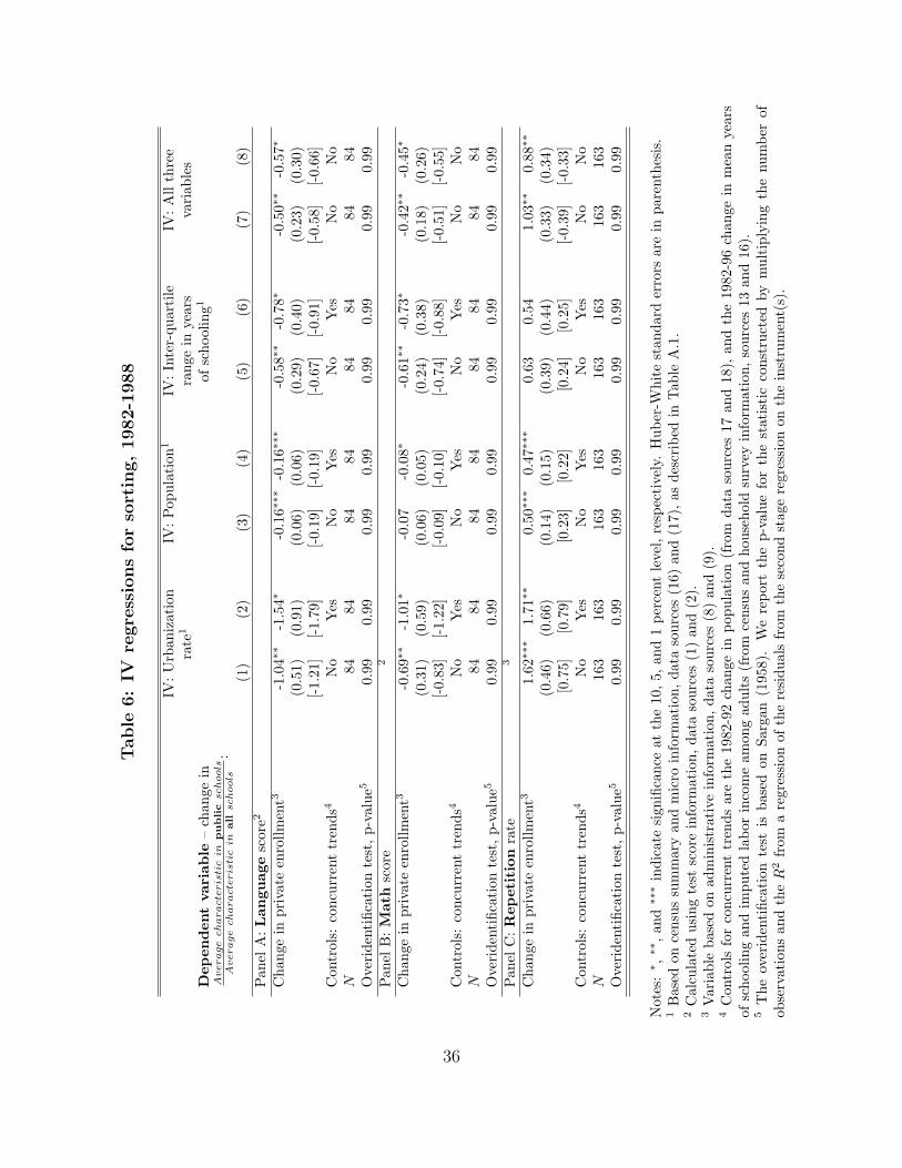
Table
6:
IVre
gre
ssio
ns
for
sort
ing,1982-1
988
IV:U
rban
izat
ion
IV:Pop
ulat
ion1
IV:In
ter-
quar
tile
IV:A
llth
ree
rate
1ra
nge
inye
ars
vari
able
sD
epen
den
tva
riab
le–
chan
gein
ofsc
hool
ing1
Average
ch
aracte
ris
tic
inpublic
sch
ools
Average
ch
aracte
ris
tic
inall
sch
ools
:(1
)(2
)(3
)(4
)(5
)(6
)(7
)(8
)Pan
elA
:Lan
guag
esc
ore2
Cha
nge
inpr
ivat
een
rollm
ent3
-1.0
4∗∗
-1.5
4∗-0
.16∗
∗∗-0
.16∗
∗∗-0
.58∗
∗-0
.78∗
-0.5
0∗∗
-0.5
7∗
(0.5
1)(0
.91)
(0.0
6)(0
.06)
(0.2
9)(0
.40)
(0.2
3)(0
.30)
[-1.
21]
[-1.
79]
[-0.
19]
[-0.
19]
[-0.
67]
[-0.
91]
[-0.
58]
[-0.
66]
Con
trol
s:co
ncur
rent
tren
ds4
No
Yes
No
Yes
No
Yes
No
No
N84
8484
8484
8484
84O
veri
dent
ifica
tion
test
,p-
valu
e50.
990.
990.
990.
990.
990.
990.
990.
99Pan
elB
:M
ath
scor
e2
Cha
nge
inpr
ivat
een
rollm
ent3
-0.6
9∗∗
-1.0
1∗-0
.07
-0.0
8∗-0
.61∗
∗-0
.73∗
-0.4
2∗∗
-0.4
5∗
(0.3
1)(0
.59)
(0.0
6)(0
.05)
(0.2
4)(0
.38)
(0.1
8)(0
.26)
[-0.
83]
[-1.
22]
[-0.
09]
[-0.
10]
[-0.
74]
[-0.
88]
[-0.
51]
[-0.
55]
Con
trol
s:co
ncur
rent
tren
ds4
No
Yes
No
Yes
No
Yes
No
No
N84
8484
8484
8484
84O
veri
dent
ifica
tion
test
,p-
valu
e50.
990.
990.
990.
990.
990.
990.
990.
99Pan
elC
:R
epet
itio
nra
te3
Cha
nge
inpr
ivat
een
rollm
ent3
1.62
∗∗∗
1.71
∗∗0.
50∗∗
∗0.
47∗∗
∗0.
630.
541.
03∗∗
0.88
∗∗
(0.4
6)(0
.66)
(0.1
4)(0
.15)
(0.3
9)(0
.44)
(0.3
3)(0
.34)
[0.7
5][0
.79]
[0.2
3][0
.22]
[0.2
4][0
.25]
[-0.
39]
[-0.
33]
Con
trol
s:co
ncur
rent
tren
ds4
No
Yes
No
Yes
No
Yes
No
No
N16
316
316
316
316
316
316
316
3O
veri
dent
ifica
tion
test
,p-
valu
e50.
990.
990.
990.
990.
990.
990.
990.
99
Not
es:∗ ,
∗∗,an
d∗∗
∗in
dica
tesi
gnifi
canc
eat
the
10,5,
and
1pe
rcen
tle
vel,
resp
ecti
vely
.H
uber
-Whi
test
anda
rder
rors
are
inpa
rent
hesi
s.1
Bas
edon
cens
ussu
mm
ary
and
mic
roin
form
atio
n,da
taso
urce
s(1
6)an
d(1
7),as
desc
ribe
din
Tab
leA
.1.
2C
alcu
late
dus
ing
test
scor
ein
form
atio
n,da
taso
urce
s(1
)an
d(2
).3
Var
iabl
eba
sed
onad
min
istr
ativ
ein
form
atio
n,da
taso
urce
s(8
)an
d(9
).4
Con
trol
sfo
rco
ncur
rent
tren
dsar
eth
e19
82-9
2ch
ange
inpo
pula
tion
(fro
mda
taso
urce
s17
and
18),
and
the
1982
-96
chan
gein
mea
nye
ars
ofsc
hool
ing
and
impu
ted
labo
rin
com
eam
ong
adul
ts(f
rom
cens
usan
dho
useh
old
surv
eyin
form
atio
n,so
urce
s13
and
16).
5T
heov
erid
enti
ficat
ion
test
isba
sed
onSa
rgan
(195
8).
We
repo
rtth
ep-
valu
efo
rth
est
atis
tic
cons
truc
ted
bym
ulti
plyi
ngth
enu
mbe
rof
obse
rvat
ions
and
the
R2
from
are
gres
sion
ofth
ere
sidu
als
from
the
seco
ndst
age
regr
essi
onon
the
inst
rum
ent(
s).
36

Tab
leA
.1:
Dat
aso
urc
es
Ori
gina
lY
ear
Dat
aty
pean
dso
urce
unit
ofob
serv
atio
n19
7019
7819
8019
8219
8819
9019
9219
9619
9819
99Tes
tsc
ores
PE
R1
Scho
ol(1
)SI
MC
E2
Scho
ol(2
)(3
)(4
)T
IMSS
3C
ount
ry(5
)In
tern
atio
nalsc
ienc
eex
ams4
Cou
ntry
(6)
Adm
inis
trat
ive
info
rmat
ion
Enr
ollm
ent
files
Scho
ol(7
)(8
)(9
)(1
0)H
ouse
hol
dsu
rvey
sC
ASE
N5
Indi
vidu
al(1
1)(1
2)(1
3)(1
4)C
ensu
sM
icro
data
Indi
vidu
al(1
5)(1
6)Su
mm
ary
files
Com
mun
e(1
7)(1
8)O
ther Sc
hool
map
s6C
omm
une
(19)
1P
rogr
ama
deE
valu
acio
nde
lR
endi
mie
nto
Esc
olar
.2
Sist
ema
deE
valu
acio
nde
Cal
idad
dela
Edu
caci
on.
3T
hird
Inte
rnat
iona
lM
athe
mat
ics
and
Scie
nce
Stud
y,se
eht
tp:/
/tim
ss.b
c.ed
u4
Inte
rnat
iona
lSc
ienc
eE
xam
s,In
tern
atio
nalE
duca
tion
Ass
ocia
tion
,se
eC
ombe
ran
dK
eeve
s(1
973)
.5
Enc
uest
ade
Car
acte
riza
cion
Soci
oeco
nom
ica
Nac
iona
l.6
See
Inst
itut
oG
eogr
afico
Mili
tar
(198
3).
37

Table A.2: Reduced form regressions for achievement, 1982-1988
Independent variable – 1982 observation of:
Urbanization Population1 Inter-quartilerate1 range in years
of schooling1
Dependent variable –1982-88 change in: (1) (2) (3) (4) (5) (6)Private enrollment2 0.09∗∗∗ 0.08∗∗∗ 0.44∗∗∗ 0.42∗∗∗ 0.19∗∗∗ 0.19∗∗∗
(0.03) (0.03) (0.07) (0.07) (0.04) (0.05)[0.32] [0.28] [0.31] [0.30] [0.38] [0.38]
Controls for trends3 No Yes No Yes No YesN 84 84 84 84 84 84R2 0.101 0.222 0.091 0.238 0.150 0.281Average Language score4 -3.5 -2.2 1.9 5.0∗∗ -3.8 -1.9
(2.4) (2.8) (2.2) (2.2) (3.5) (3.8)[-0.18] [-0.11] [0.02] [0.05] [-0.11] [-0.06]
Controls for trends3 No Yes No Yes No YesN 84 84 84 84 84 84R2 0.031 0.113 0.000 0.105 0.012 0.106Average Math score4 -9.0∗∗∗ -8.2∗∗∗ -3.5 -0.4 -11.0∗∗∗∗ -8.8∗∗
(2.2) (2.4) (3.0) (3.1) (3.6) (4.0)[-0.43] [-0.39] [-0.03] [-0.00] [-0.30] [-0.24]
Controls for trends3 No Yes No Yes No YesN 84 84 84 84 84 84R2 0.182 0.277 0.001 0.144 0.091 0.194Average Repetition rate2 0.04∗∗∗ 0.04∗∗∗ 0.09∗∗ 0.08∗∗ 0.06∗∗∗ 0.06∗∗∗
(0.01) (0.01) (0.04) (0.04) (0.02) (0.02)[0.34] [0.34] [0.09] [0.08] [0.26] [0.26]
Controls for trends3 No Yes No Yes No YesN 145 145 145 145 145 145R2 0.119 0.151 0.009 0.078 0.085 0.122Mean years of schooling5 -0.5∗∗∗ -0.7∗∗∗ -1.0∗∗ -1.2∗∗ -0.8∗∗ -0.7∗∗
(0.2) (0.2) (0.5) (0.5) (0.3) (0.3)[-0.26] [-0.37] [-0.09] [-0.11] [-0.22] [-0.19]
Controls for trends3 No Yes No Yes No YesN 85 85 85 85 85 85R2 0.077 0.326 0.007 0.239 0.043 0.261
Notes: ∗, ∗∗, and ∗∗∗ indicate significance at the 10, 5, and 1 percent level, respectively. Huber-Whitestandard errors are in parenthesis. Brackets contain the proportion of a std. dev. change in the dependentvariable brought about by a one std. dev. increase in the private enrollment rate.1 Based on census summary and micro information, data sources (16) and (17), as described in Table A.1.2 Calculated using administrative information, data sources (8) and (9)3 Controls for pre-existing and concurrent trends, as described in Table 3, notes 4 and 5.4 Based on test score information, data sources (1) and (2).5 Calculated using census and household survey information, data sources (16) and (11).
38

Table A.3: Reduced form regressions for sorting, 1982-1988
Independent variable:
Urbanization Population1 Inter-quartilerate1 range in years
of schooling1
Dependent variable –1982-88 change in: (1) (2) (3) (4) (5) (6)Private enrollment2 0.08∗∗ 0.06∗∗ 0.44∗∗∗ 0.41∗∗∗ 0.16∗∗∗ 0.15∗∗∗
(0.03) (0.03) (0.05) (0.05) (0.04) (0.04)[0.31] [0.23] [0.33] [0.31] [0.36] [0.34]
Controls: concurrent trends3 No Yes No Yes No YesN 84 84 84 84 84 84R2 0.104 0.183 0.110 0.228 0.138 0.220Sorting measure for Language4,5 -0.09∗∗∗ -0.10∗∗∗ -0.07∗∗ -0.06∗∗ -0.09∗∗ -0.11∗∗
(0.03) (0.03) (0.03) (0.03) (0.04) (0.05)[-0.40] [-0.45] [-0.06] [-0.05] [-0.24] [-0.29]
Controls: concurrent trends3 No Yes No Yes No YesN 84 84 84 84 84 84R2 0.151 0.171 0.004 0.011 0.062 0.080Sorting measure for Math4,5 -0.06∗∗∗ -0.06∗∗ -0.03 -0.03 -0.10∗∗∗ -0.11∗∗
(0.02) (0.03) (0.02) (0.02) (0.04) (0.05)[-0.28] [-0.28] [-0.02] [-0.03] [-0.28] [-0.30]
Controls: concurrent trends3 No Yes No Yes No YesN 84 84 84 84 84 84R2 0.073 0.128 0.001 0.052 0.076 0.120Sorting measure for Repetition2,4 0.17∗∗∗ 0.14∗∗∗ 0.28∗∗ 0.07 0.25∗∗ 0.09
(0.04) (0.05) (0.11) (0.10) (0.08) (0.07)[0.31] [0.26] [0.03] [0.02] [0.11] [0.09]
Controls No Yes No Yes No YesN 163 163 163 163 163 163R2 0.100 0.130 0.003 0.076 0.014 0.080
Notes: ∗, ∗∗, and ∗∗∗ indicate significance at the 10, 5, and 1 percent level, respectively. Huber-Whitestandard errors are in parenthesis. Brackets contain the proportion of a std. dev. change in the dependentvariable brought about by a one std. dev. increase in the private enrollment rate.1 Based on census summary and micro information, data sources (16) and (17), as described in Table A.1.2 Based on administrative information, data sources (8) and (9)3 Controls for concurrent trends are the 1982-92 change in population (data sources 17 and 18), and the1982-96 change in mean years of schooling among adults, and imputed labor income (from census andhousehold survey information, sources 13 and 16).4 The sorting measure is Average characteristic in public schools
Average characteristic in all schools .5 Based on test score information, data sources (1) and (2).
39

Figure 1: National enrollment shares by sector, 1970-19951
0
10
20
30
40
50
60
70
80
90
70 71 72 73 74 75 76 77 78 79 80 81 82 83 84 85 86 87 88 89 90 91 92 93 94 95 9
Enr
ollm
ent s
hare
by
type
of s
choo
l
Fiscal
Total private
Totalprivate
Municipal
Voucher private (previously subsidized private)
Tuition-charging private
Figure 2: Private enrollment among communes2
Panel A: Within-commune changes, 1982-96.
All communes Urban communes
-.2 0 .2 .4 .600
Panel B: Levels, 1996.
All communes Urban communes
0 .5 100
1 Data assembled from several issues of the Ministry of Education’s Compendio Estadístico. 2 Panel A is based on administrative information, data sources (8) and (10) in Table A.1. It covers all communes in Chile. Panel B refers to communes with positive private enrollment.

Figure 3: Number of schools by sector, 1980-19951
0
1,000
2,000
3,000
4,000
5,000
6,000
1980 1985 1990 1995
Num
ber
of sc
hool
s
Municipal
Voucher private
Tuition-charging private
1 Data assembled from several issues of the Ministry of Education’s Compendio Estadístico.

Figure 4: Chile’s Performance in International Tests, 1970 and 1999
A. Median Test Scores (standard deviation from 13-country average). ..
.19
99
.1970
-1 -.5 0 .5 1
-1
-.5
0
.5
1
IRN
CHL
THA
NLD
ITA
FINBELGBR
USA NZL
AUSHUN JPN
B. Residual Median Test Scores (standard deviation from 13-country average)
.
.
.19
99
.1970
-1 -.5 0 .5 1-1
-.5
0
.5
1
ITA
IRNBELNZLTHAGBR
CHL
HUNNLDUSA
AUSFINJPN
Note: The scores for each country subtract the mean score for the 13 countries and are divided by the standard deviation of U.S. scores in the given year. Residual test scores are residuals from regression of median test score on GDP/worker, enrollment rate, and ratio of spending per student to GDP per capita.

Figure 5 Average test score among municipal and voucher schools, relative to tuition-charging
private schools, 1982 and 1996 (Std. Deviations below tuition charging)
-1.60
-1.40
-1.20
-1.00
-0.80
-0.60
-0.40
-0.20
0.001982 1996
math spanish