Junk Food in Schools and Childhood Obesity Much Ado About Nothing?

ASHLESHA DATAR, NANCY NICOSIA

WR-672

March 2009

WORK ING P A P E R

This product is part of the RAND Health and RAND Labor and Population working paper series. RAND working papers are intended to share researchers’ latest findings and to solicit informal peer review. They have been approved for circulation by RAND Health and RAND Labor and Population but have not been formally edited or peer reviewed. Unless otherwise indicated, working papers can be quoted and cited without permission of the author, provided the source is clearly referred to as a working paper. RAND’s publications do not necessarily reflect the opinions of its research clients and sponsors.

is a registered trademark.

1

Junk Food in Schools and Childhood Obesity: Much Ado About Nothing?

Ashlesha Datar* and Nancy Nicosia

February 2009

Abstract

There is a growing belief among policymakers and the general public that competitive foods in schools are a significant contributor to the childhood obesity epidemic. Numerous policy initiatives are underway at the local, state and federal level to regulate the availability of competitive foods in schools. However, the existing empirical evidence motivating these efforts is limited and rarely addresses the potential endogeneity of the school food environment. In this paper, we estimate the causal effect of competitive food availability on children’s body mass index (BMI) and other food- and school-related outcomes using an instrumental variables approach on a national sample of children. We find that competitive food availability generates in-school purchases of junk foods, but contrary to common concerns, there is no significant effect on children’s BMI. Nor do we observe significant changes in overall consumption of healthy and unhealthy foods, and in physical activity. Finally, our results find no support for broader effects of junk foods in school on social/behavioral and academic outcomes.

*Corresponding author, RAND Corporation, 1776 Main Street, P.O. Box 2138, Santa Monica, CA 90407, Email: datar@rand.org This research was funded by grants from the Robert Wood Johnson Foundation’s Healthy Eating Research Program, NIH R01 HD057193, the Bing Center for Health Economics at RAND, and the RAND Labor and Population Program. All opinions are those of the authors and do not represent opinions of the funding agencies. We are grateful to Darius Lakdawalla, Neeraj Sood, Roland Sturm for their helpful comments, and to Carlos Dobkin and Eric Meijer for helpful discussions. We are also grateful to Le Wang for sharing his STATA code to estimate quantile regression instrumental variables models. All remaining errors are our own.

2

1. Introduction

The prevalence of childhood obesity in the US is at an all-time high with nearly

one-third of all children and adolescents now considered overweight or obese (Ogden et

al 2008). Considerable attention has been focused on schools in an attempt to identify

policy levers that will help reverse the obesity epidemic. In particular, the availability of

“competitive foods” in schools, defined as foods and beverages available or sold in

schools outside of the school lunch and breakfast programs, has been a much debated

issue.

Competitive foods are sold through a la carte lines, vending machines, school

canteens/stores, and fundraisers and, in contrast to the federally-reimbursable school

meal programs, there are no federal nutritional standards for foods sold through these

venues. As a result, competitive foods account for much of the variation in the food

environment across schools. On the one hand, opponents question the nutritional value

of competitive foods, and indeed, the available evidence suggests that competitive foods

are higher in fat compared with foods sold as part of the school meal programs (Gordon

et al 2007b, Harnack et al 2000, Wechsler et al 2000, Story, Hayes & Kalina 1996). On

the other hand, supporters argue that revenues from these food sales provide much-

needed funding for schools, especially in times of budgetary pressures. For example,

during 2005-2006, middle and high schools earned an average of $10,850 and $15,233,

respectively, from a la carte sales alone.1 In addition, nearly a third of high schools and

middle schools earned between $1,000-$9,999 during that same year, another ten

percent earned between $10,000-$50,000, and a small number earned in excess of

1 Estimates are based on the 2005 School Nutrition and Dietary Assessment Study (SNDA-III), but response rates were low for some revenue categories (Gordon et al 2007a). Competitive food availability and revenues were less common in elementary schools though as many as 47% of elementary schools have pouring rights contracts.

3

$50,000 per year. These figures are substantial and may be supplemented by additional

revenue from on-site school stores and pouring contracts with beverage companies.

Competitive foods availability is a long-standing issue in the policy debate.

Legislation and regulations targeting competitive foods have been proposed for

decades. U.S. Department of Agriculture (USDA) regulations had been comprehensive,

but in 1983, a successful lawsuit by the National Soft Drink Association limited the scope

of these regulations to food service areas during meal hours. In recent years, several

states, school districts, and individual schools have enacted competitive food policies

that are more restrictive than federal regulations.2 For example, two of the largest school

districts in the nation, New York City Public School District and Los Angeles Unified

School District, imposed a ban on soda vending in schools in 2003 and 2004,

respectively. Many others have followed suit with similar bans or stricter regulation of

competitive foods.

Despite the growing support for competitive food regulation, it is hard to deny

opponents’ claims that the evidence against competitive foods is limited. Existing

research does show that competitive food availability in schools is associated with a

decline in nutritional quality of meals consumed at school (Cullen et al 2000, Cullen &

Zakeri 2004; Templeton, Marlette & Panemangalore 2005).3 However, less is known

about the effects on overall diet quality (consumed in and out of school) and children’s

weight. The literature does provide some evidence of substitution of caloric intake

across meals and location among adults (Anderson and Matsa 2009), but the evidence

is less clear regarding children. Only Kubik and colleagues have examined 24 hour

dietary recall (2003) and BMI (2005), however these studies are generally based on

2 Competitive food policies differ widely in the types and stringency of restrictions they apply. 3 Other studies have examined the effects of price reductions and increases in availability and promotion of low-fat foods in secondary schools on sales and purchases of these foods (French et al 2004, 2001, 1997a, 1997b, Jeffery et al 1994) as well as their consumption (Perry et al 2004) within experimental settings and have found positive effects.

4

small local samples and do not address the potential endogeneity of the school food

environment.4 An exception is Anderson and Butcher (2006), who use national data on

adolescents to examine whether school food policies such as the availability of “junk

foods”, “pouring rights” contracts, soda and snack food advertisements, and school

events have an impact on adolescent obesity. 5 In the absence of a single data source

containing information on school food policies and BMI, the authors use a two-sample

instrumental variables (IV) approach to estimate the effects of school food policies on

adolescent BMI. Using county, state, and regional characteristics as instruments that

capture budgetary pressures on schools, they find that a 10 percentage point increase in

the proportion of schools in the county that offer junk foods leads to a 1 percent increase

in BMI. This effect is primarily driven by adolescents with an overweight parent, which

the authors interpret as a measure of family susceptibility to weight gain. Their results for

the other school policies, pouring rights contracts, and food and beverage

advertisements are smaller and less precise. The IV approach constitutes an innovation

over the literature, but the authors acknowledge that their results may be undermined by

a weak first stage.

Our paper adds to the limited existing literature by attempting to isolate the

causal effect of competitive food availability on children’s food consumption and BMI

using data on a national sample of fifth graders from the Early Childhood Longitudinal

4 Kubik et al (2003) find that a la carte availability in school is negatively associated with overall intake of fruits and vegetables and positively associated with total and saturated fat intake among 7th graders attending 16 schools in Minneapolis-St Paul. Using the same data, Kubik et al (2005) show that practices such as the use of competitive foods as rewards and incentives for students are positively associated with higher body mass index (BMI). 5 “Junk Food Available” means that students can buy chocolate, candy, cakes, ice cream, or salty snacks (that are not fat free) from a machine or school store. “Pouring Rights” contract means the school has agreed to sell one brand of soft drinks, often in exchange for a percentage of sales or other incentive packages. “Soda or Snack Food Advertisements” means that advertisements are allowed at least at one type of school related activity or in one or more places at the school—for example, on a school bus, at a school sporting event, on school grounds, or school textbooks etc.

5

Study – Kindergarten Class (ECLS-K).6 We leverage the well-documented fact that

competitive foods are significantly more prevalent in middle and high schools relative to

elementary schools (Finkelstein, Hill and Whitaker 2008).7 Exogenous variation in

competitive food availability across schools is identified using the grade structure in the

child’s school. We argue that a fifth grader attending a combined (e.g. K-8, K-12) or

middle school (e.g. 5-8) is more likely to be exposed to competitive foods compared to a

fifth grader in an elementary school (e.g. K-5 or K-6), but that the school’s grade

structure has no direct effect on a child’s weight. First-stage regressions,

overidentification tests, checks for peer effects, and ”placebo” regressions on children’s

outcomes in kindergarten indicate that the instruments are valid and strong predictors of

competitive food availability.

We find that competitive food availability generates in-school purchases of junk

foods, but contrary to common concerns about these foods, there is no statistically or

economically significant effect on BMI. While our IV estimates tend to be less precisely

estimated, Hausman tests can not reject the consistency of OLS estimates that are

precisely estimated. In-school purchases of junk food typically provide up to an

additional 22 calories per day among children who have access to competitive foods and

62 calories per day among children who purchase these foods at school.8 The caloric

contribution of such foods among children who purchase amounts to 3.5 percent of the

estimated daily caloric requirements for a moderately active fifth grader and less than a 6 In a recent paper, Fernandes (2008) also used data from the Early Childhood Longitudinal Study to examine the correlation between soft drink availability and in-school and overall consumption of soft drinks among fifth graders and found a small positive association. However, the study did not address the endogeneity of school food environment and was only restricted to examining soda consumption. 7 According to the SNDA-III, as many as 97% of high schools and 82% of middle schools had vending machines compared to only 17% of elementary schools. About 60% of high schools, 50% of middle schools, and 37% of elementary schools had fundraising activities involving sale of sweet or salty snacks (Gordon et al 2007b). 8 The difference in caloric contribution of in-school purchases is lower for children with access to junk foods relative to children who actually purchase these foods at school because up to half of those who have access choose not to purchase.

6

quarter of their daily discretionary calorie allowance.9 It is not surprising, therefore, that

competitive foods do not appear to significantly increase BMI. Ancillary regressions of

students’ eating behavior provide evidence to support this finding. The total amount of

soda and fast food, consumed in- and out-of-school, is not significantly influenced by

competitive food availability, which is consistent with substitution between in-school and

out-of-school consumption. In general, we also find no deleterious effects on the total

consumption of various healthy foods. Our evidence suggests that the lack of impact on

BMI is not likely explained by compensatory changes in children’s physical activity.

Finally, we examine whether junk food adversely affects social/behavioral and academic

outcomes in fifth grade and find that no evidence of detrimental effects on these

outcomes.

The remainder of this paper is organized as follows. Section 2, describes our

data and relevant analysis variables. In Section 3, we describe our empirical strategy,

which implements an instrumental variables approach and leverages longitudinal

information on BMI to identify the causal impact of competitive food availability. In

Section 4, we discuss our results for children’s BMI and test the robustness of our

results. We also present ancillary regressions examining the effects of competitive food

availability on food consumption and physical activity. We end this section with an

examination of broader effects of competitive food availability on children’s

social/behavioral outcomes and academic performance in fifth grade. Finally, Section 5

concludes with the policy implications of our findings.

9 See Dietary Guidelines for Americans 2005 for information on estimated daily caloric needs by age and gender <http://www.health.gov/dietaryguidelines/dga2005/document/html/chapter2.htm#table3> accessed 22 August 2008. Discretionary calories are those calories that can be used ‘at your discretion’ after basic nutrition needs are met without exceeding energy requirements. It is the difference between an individual’s total energy requirement and the energy (calories) they consume to meet nutrient requirements. According to the Dietary Guidelines for Americans 2005, the discretionary calorie allowance for a 2000 calorie diet is 267 calories.

7

2. Data

We use data on fifth graders from the Early Childhood Longitudinal Study –

Kindergarten Class (ECLS-K). The ECLS-K is a panel dataset on a nationally

representative cohort of kindergarteners in the U.S. who entered school in fall 1998.

The study surveyed this cohort in kindergarten, first, third, and fifth grades collecting

information from children and their parents, teachers, and schools on children's

cognitive, social, emotional, physical development, and their home, classroom, and

school environments.10 However, information on the school’s food environment and

children’s food consumption was collected only in the fifth grade. Our analysis sample

includes approximately 10,000 children attending the fifth grade in public and private

schools in the 2003-04 school year. Below, we describe the key variables for our

analyses. Descriptive statistics of all the variables used in the analyses are provided in

Tables 1 and 2.

2.1. Dependent Variables

Body Mass Index (BMI): A distinct advantage of the ECLS-K is that it collected

height and weight measurements from children at kindergarten entry and at each

subsequent data collection round. These data are superior to self- or parent-reported

height and weight data that may introduce non-random measurement error. The height

and weight measurements are used to compute children’s BMI, defined as weight in

kilograms divided by height in meters squared. We use log of BMI in fifth grade as the

10 The ECLS-K sample was freshened in the first grade therefore the sample of children in the fifth-grade round represents the cohort of children who were in kindergarten in 1998–99 or in first grade in 1999–2000.

8

dependent variable in the regressions. The average BMI in our sample of fifth graders is

20.4.11

Junk Food Purchase in School: The fifth grade child food consumption

questionnaire collected information on children’s junk food purchase in school during the

pervious school week. These questions asked about the frequency (times per week) of

purchase of sweets (candy, ice cream, cookies, brownies or other sweets), salty snack

food (potato chips, corn chips, Cheetos, pretzels, popcorn, crackers or other salty

snacks), and sweetened beverages (soda pop, sports drinks or fruit drinks that are not

100 percent juice). Table 2 panel A shows the frequency distribution of in-school junk

food purchases. A large majority of the children did not purchase junk food in school

during the reference week - 77 percent for sweets, 84 percent for salty snacks, and 88

percent for sweetened beverages – in large part because the majority of students did not

have the opportunity to do so (see Section 2.2). Conditional on availability in school,

about half the sample purchased any of these foods at least once a week. Further,

among those who did purchase, the modal response was 1-2 times per week – 68

percent for sweets, 72 percent for salty snacks, and 70 percent for sweetened

beverages.

Total Consumption of Selected Foods and Beverages: The child food

consumption questionnaire asked about the “total consumption” of two unhealthy and

seven healthy foods/beverages during the past 7 days. The two unhealthy items

included – (a) soda pop/sports drinks/fruits drink that are not 100 percent juice

(hereafter, referred to as “soda”), and (b) fast food. The seven healthy food items

included – (a) milk, (b) 100 percent fruit juices, (c) green salad, (d) potatoes12, (e)

11 We also estimate separate models for whether the child is obese in fifth grade, defined as BMI greater than the 95th percentile for age and gender on the Center for Disease Control (CDC) growth charts. About 20 percent of our sample is obese. 12 The “potatoes” category excluded French fries, fried potatoes, and potato chips.

9

carrots, (f) other vegetables, and (g) fruits. Children were asked to include in their

responses foods they ate at home, at school, at restaurants, or anywhere else (See

Appendix 3 for exact language of the questions). Table 2, panel B shows the frequency

distribution of total consumption of these food groups. In the unhealthy foods category,

the percentage of children not consuming any soda or fast foods during the previous

week was 16 and 29 percent, respectively. Children consumed soda more frequently

than fast food. In the healthy foods category, green salad, carrots and potatoes were

consumed most infrequently with 45-49 percent children never consuming them in the

past 7 days. The modal response for the other healthy food groups was 1 to 3 times in

the past 7 days.

2.2. Competitive Food Availability

Information on competitive food availability in schools was collected only in the

fifth grade wave of the ECLS-K. This information was obtained from two sources - school

administrator and child questionnaires (See Appendix 3 for exact language of the

questions). The school administrator questionnaire asked about the presence of

alternate competitive food outlets, including vending machines, school stores, canteens,

snack bars, and a la carte lines. The school administrators were also asked about the

availability of specific food items during school hours through any of the venues. These

items included candy, high-fat salty snacks, low-fat salty snacks, high-fat baked goods,

low-fat baked goods, ice cream, milk, fruits/vegetables, bottled water, 100 percent juice,

and soda pop or other beverages that are not 100 percent juice. The child food

consumption questionnaire asked if sweets, salty snacks, and sweetened beverages

could be purchased at the school during school hours. Based on these questions we

constructed three alternate measures of competitive food availability in the school.

10

1. School Administrator-Reported Junk Food Availability: equals 1 if students

can purchase any of the following - candy, chocolate, foods containing sugar, salty

snacks, ice cream or frozen yogurt, or sweetened beverages (soda pop, sports

drinks, or fruit drinks that are not 100 percent juice) - and zero otherwise. About 61

percent of the sample reported junk food availability in school based on the school

administrator report.

2. Child-Reported Junk Food Availability: equals 1 if child reports that foods

containing sugar, salty snacks, or sweetened beverages can be purchased at school

during school hours. About 72 percent of the children reported junk food availability

in their school.

3. Competitive Food Outlet: equals 1 if any of the following competitive food outlets

are present in the school - vending machines, school stores, canteens, snack bars,

and a la carte lines – and 0 otherwise. About 60 percent of the sample had any

competitive food outlet, based on school administrator reports.

The first two measures capture the availability of junk foods in school regardless of

their source whereas the third measure captures the presence of unregulated food and

beverage outlets in schools regardless of the type of food they sell. This distinction is

useful for two reasons. First, even though competitive food venues have been largely

blamed for junk food availability these foods may also be available as part of school

meals. And second, unregulated outlets in schools may not always (or only) sell junk

foods. The first two measures should capture the same availability, but there is

disagreement for a quarter of the sample.13 This discrepancy could result from

differences in survey timing of the school administrator and child questionnaires, recall

13 About 18 percent of the children report junk food being available in their school but the school administrator reports otherwise, and about 7 percent of the children report no junk food availability in their school even though the school administrator reports otherwise.

11

problems, or due to differences in perceptions about whether foods sold during

fundraising activities should be included in the response.14

3. Empirical Approach

3.1. Econometric Model

The relationship between competitive food availability and child outcomes in fifth

grade can be estimated using the following linear regression model.

(1) Yik = 0 + 1 CFk + 2 Xik + 3 Sk + ik

where, Yik, denotes fifth grade BMI (or other outcomes) for child i in school k, CFk is a

measure of competitive food availability in the child’s school, Xik and Sk are the vectors

of individual/family (gender, race/ethnicity, mother’s education, household income) and

school characteristics (private/public, percent minority, enrollment, urbanicity,

state/region), respectively, and ik is the error term. The parameter of interest is 1.

Obtaining an unbiased estimate of 1 is challenging because the school food

environment is not exogenous to the outcomes of interest. Schools that serve high-fat,

energy-dense competitive foods may differ on many observable and unobservable

factors that are correlated with children’s weight and dietary behavior. In particular, the

decision to offer competitive foods in schools may be influenced by a variety of factors

including budgetary pressures, demands of the student population, parental

involvement, and state/district policies. These factors could independently influence

children’s weight as well. For example, budgetary pressures may induce schools to

scale back or eliminate physical education programs, which might increase children’s

weight. As a result, coefficient estimates from the ordinary least squares (OLS)

estimation of Equation 1 would be biased.

14 School administrators were not asked about foods sold at fundraising events, but children were asked about availability of specific foods anywhere in the school.

12

3.2. Addressing Endogeneity of Competitive Food Availability in Schools

We address the endogeneity of competitive food availability using state fixed

effects and state fixed effects with IV models. We also control for children’s BMI at

school entry (kindergarten) to account for any pre-exposure differences in BMI across

children. 15

Our first specification is similar to Equation 1, but adds state fixed effects ( s) and

baseline (kindergarten) BMI (BBMIiks) (Equation 2).

(2) Yiks = 1 CFks + 2 Xiks + 3 Sks + 4 BBMIiks + s + iks

States differ markedly in terms of obesity prevalence in their populations as well as the

policy environment geared towards combating obesity. State fixed effects control for

state-specific time-invariant unobserved heterogeneity that may be correlated with

school food environments and children’s weight. The child’s baseline BMI at

kindergarten is included to address some of the endogeneity issues that can bias OLS

estimates such as student demand for competitive foods, genetic susceptibility, and

sorting.16

The specification in equation (2), however, may still not result in unbiased

estimates if within-state variation may be endogenous even after the inclusion of

baseline BMI. For example, districts may choose to set more or less restrictive policies

than the state requires due to differences in budgetary pressures. To isolate the

exogenous component, we construct instrumental variables for within-state variation in

competitive food availability using information on the grade span in each child’s school.

15 The ECLS-K also provides BMI measured in the third grade, which we include as a sensitivity analysis. 16 Because competitive food availability data are collected only in fifth grade, we do not know the length of exposure – that is, whether the child has had competitive foods available throughout elementary school or whether a change in the school attended or a change in school policy altered exposure. Therefore, BMI in kindergarten is used as a control since it is measured prior to exposure to competitive foods in school.

13

Equation 3.1 represents the first-stage regression where competitive food

availability is regressed on the grade span instrument, individual and school

characteristics, baseline BMI, and state fixed effects. Equation 3.2 represents the

second stage where children’s BMI is regressed on the predicted availability of

competitive foods from the first stage in addition to the common covariates.

(3.1) CFks = 1 GradeSpanks + 2 Xijs + 3 Sks + 4 BBMIiks + s + iks

(3.2) Yiks = 1 Fks + 2 Xijs + 3 Sks + 4 BBMIiks + s + iks

3.2.1. Instruments

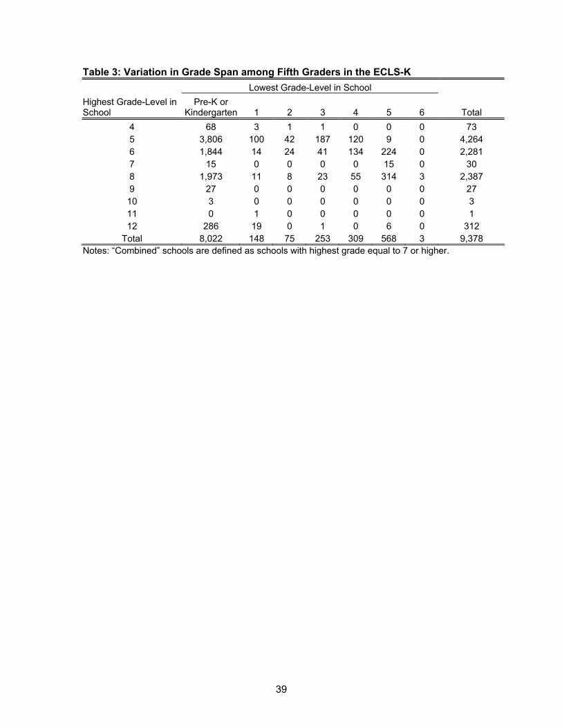
Our sample consists of a single cohort of fifth graders attending schools with a

variety of grade spans .Given that competitive food availability is significantly higher in

middle and high schools compared to elementary schools, a potentially useful instrument

for competitive food availability is whether the fifth grader is in a combined/middle school

(i.e. defined as a school where the highest grade is seventh or higher) or whether the

fifth grader is in an elementary school (i.e. highest grade is fifth or sixth). Our main

instrument considers only the school type: elementary versus middle/combined

(hereafter, middle/combined is referred to only as “combined”). Over 70 percent of our

sample attends a elementary school defined as grades K-5 or K-6 (see Table 3). The

remainder attend combined schools, mainly schools with grades K-8 (8 percent), grades

K-12 (2 percent) and grades 5-8 (4 percent). In alternate regressions, we also leverage

information on the lowest and highest grades in a child’s school and conduct

overidentification tests.

For grade structure to be a valid instrument for competitive food availability, it

must be the case that having older peers in the school has no direct effect on children’s

weight. In other words, the presence of older students in the school should only affect

the weight of younger students through the school’s food environment.

14

Peers, defined broadly, have been shown to influence a wide range of

adolescent behaviors and outcomes including substance abuse, academic achievement,

social and behavioral outcomes, and food choices.17 Of particular relevance to our

identification strategy, however, is the literature examining a specific type of peer effect,

namely, the effect of exposure to older or younger peers due to school grade span on

adolescent behaviors and outcomes. The evidence to date is mixed. Using variation in

school grade span to identify peer effects, Clark and Folk (2007) find that sixth graders

who attend middle school are significantly more likely to smoke, drink, use drugs

compared to sixth graders who attend elementary school. But Eisenberg (2004) finds

that seventh and eighth graders who attend schools with older peers are no more likely

to use substances relative to those who attend schools with younger peers.18

Other studies have directly examined the effect of grade span on academic

performance and social/behavioral outcomes (Bedard and Do 2005; Cook et al 2008).

This literature has primarily focused on whether middle school settings are better or

worse than either elementary or combined school settings. A consistent finding is that

sixth or seventh graders who attend middle school have poorer academic and behavioral

outcomes compared to those who attend elementary or combined schools. However, we

are not aware of any studies that compare achievement of a single cohort of children in

a particular grade across elementary and combined schools. The exception is Rickles

(2005), whose findings suggest inconsistent effects of grade span on achievement.

17 This literature has examined peer effects on a wide range of outcomes including substance use (Clark and Folk 2007; Clark and Loheac 2007; Lundborg 2006; Eisenberg 2004; Case and Katz 1991; Gaviria and Raphael 2001), crime (Case and Katz 1991; Glaeser, Sacerdote, and Scheinkman 1996; Regnerus 2002), teenage pregnancy (Crane 1991; Evans, Oates and Schwab 1992), discipline (Cook et al 2008), and academic achievement (Hoxby 2000; Hanushek et al 2003; Cook et al 2008), and adolescent food choices (Perry, Kelder, Komro 2003; Cullen et al 2001; French et al 2004) and weight (Trogdon, Nonnemaker and Pais 2008). 18 Clark and Loheac (2007) find that substance use behavior of students within the same school who are one year older influences adolescent substance use.

15

There is limited evidence on the influence of older peers on food choices.19

Cullen and Zakeri (2004) compared changes in food consumption of fourth graders who

transitioned to middle school in fifth grade and gained access to school snack bars to

changes in food consumption of fifth graders who were already in middle school. Fourth

graders who transitioned to middle school consumed fewer healthy foods compared with

the previous school year, but it is not clear whether this was due to the presence of older

peers or the change in school food environment.

The evidence described above suggests that any potential bias in our estimates

is likely to be upward; fifth graders might emulate older peers who are more likely to

consume junk foods in school and would therefore tend to be overweight, independent of

the school food environment. As a result, an insignificant finding is unlikely to be

undermined.

3.2.2. Checks for Instrument Validity

Identification in our models relies on the assumption that attending a combined

school compared to an elementary school does not influence BMI except through

changes in the availability of competitive foods. We demonstrate the validity of our

instruments in a number of ways.

First, for each measure of competitive food availability, we report first-stage

estimates from one exactly identified and one overidentified model (Table 4). The

exactly-identified model uses an indicator for whether the child attends an elementary or

combined school as the instrument. The over-identified model uses two continuous

variables capturing the highest and lowest grade levels in the child’s school as

instruments. The first-stage estimates shown that presence of higher grades in the

19 To our knowledge, there are no studies that have examined the influence of younger peers on food choices and weight.

16

school significantly increases the likelihood of competitive food availability. The F-

statistics on the instruments are larger than 20 in all cases. Moreover, the

overidentification tests do not reject the exogeneity of the instruments.

Despite this strong support, we might be concerned that there is some selection

that would confound our instrument. We test for differences in BMI and other child

outcomes in kindergarten across elementary and combined schools (Table 5 Panel A).

Because kindergarten outcomes are determined prior to exposure to the school food

environment, such comparisons would allow us to test for selection into elementary

versus combined schools. This exercise is conducted separately for public and private

school samples because combined schools are much more likely to be private. For both

public and private school students, we find no differences in unadjusted means of

children’s kindergarten BMI across elementary versus combined schools. There are

slight differences in other kindergarten outcomes: slightly higher reading (public and

private) and math scores (private only), and slightly fewer internalizing behavior

problems (private only). There are also statistically significant differences in individual,

family and school characteristics, but no overall pattern that would appear to threaten

validity of the IV approach (Table 5 Panel B). When we control for these covariate

differences in a regression context, we find that the slight differences that appeared in

the unadjusted means of kindergarten outcomes disappear (Table 6). These results

suggest that, conditional on observed background characteristics, the instrument is

uncorrelated with pre-exposure BMI, social/behavioral outcomes and test scores.

Another potential concern is that attending a combined school might generate

peer effects on BMI and food consumption, independent of competitive food availability.

We test for the presence of peer effects by regressing BMI and food consumption in fifth

grade on the instrument and other covariates using only the sample of schools that do

not offer any competitive foods (Table 7). The point estimates are very small and

17

statistically insignificant despite being precisely estimated, thus indicating the absence of

any peer effects on BMI and food consumption.

4. Results

We begin with our main results examining the effects of competitive food

availability on BMI (Section 4.1). We first estimate basic models of BMI, then augment

with state fixed effects and baseline BMI to address omitted variable bias and selection,

and finally estimate the IV specifications. In Section 4.2, we examine the sensitivity of

our main BMI results to alternate sample restrictions and report results from a

falsification test. In Section 4.3, we describe results from ancillary regressions that

explore the potential mechanisms underlying our BMI findings. In particular, we examine

in-school and total consumption of selected foods and beverages and the availability of

and participation in physical activity. Finally, in Section 4.4 we examine whether

competitive food availability influences other school outcomes such as social-behavioral

outcomes and academic achievement.

4.1. BMI

Our main results focus on whether the availability of competitive foods increases

BMI among fifth graders (Table 8). We estimate BMI as a function of the three

measures of competitive food availability at the child’s school: 1) school administrator-

reported availability, 2) child-reported availability, and 3) competitive food outlets.

Column 1 shows the results of a basic OLS regression of BMI on competitive food

availability as well as child, household, and school characteristics.20 Consistent with the

literature, the OLS regression yields a statistically significant increase in BMI for two of

the three measures of availability, although the point estimates are small. The inclusion 20 In all models, we estimate robust standard errors clustered at the school level.

18

of state fixed effects (Column 2) and a “baseline” BMI measured when the children were

in kindergarten (Column 3) eliminates the significant coefficient for all measures of

competitive food availability.21 These fully-specified OLS models have very small,

precisely estimated, and statistically insignificant point estimates that call into question

the hypothesized relationship between competitive food availability and increases in

children’s BMI.

However, the coefficients from these models may be biased if competitive food

availability is related to unobserved determinants of children’s BMI. For example,

districts with a large population of students at risk for obesity may have adopted more

stringent competitive food policies that reduce the availability of junk foods in school. In

this situation, OLS regression on cross-sectional data may show no significant

relationship or even a negative relationship between junk food availability in school and

student BMI. Another potential problem with the OLS estimates is that they might suffer

from attenuation bias due to the presence of measurement error in the competitive food

availability measures.

To address these issues, we estimate Two Stage Least Squares (2SLS)

regressions using two measures of grade span as instruments: (1) whether the fifth-

grader attended a combined school with older peers in grades 7 and higher (Column 4)

and (2) the lowest and highest grade level in the child’s school to measure the presence

of younger and older peers (Column 5).22 As discussed in the previous section, both

instruments appear quite strong in the first stage with F-statistics exceeding 20 for each

availability measure. The 2SLS point estimates are relatively larger compared to the

21 In alternate models we included third grade BMI instead of kindergarten BMI as our measure of baseline BMI and our results remained the same. 22 In the remainder of the sections, we report estimates only from the exactly-identified 2SLS models since these are less subject to weak instruments critique relative to over-identified models (Angrist and Pischke 2009).

19

OLS estimates but are less precisely estimated rendering them statistically insignificant

as well. Even if the 2SLS estimates were statistically significant, they would represent a

minor increase in BMI, generally less than 1 to 2 percent. Hausman tests that check for

endogeneity of competitive food availability by comparing estimates from OLS

regressions (Column 3) with those from 2SLS models (Columns 4 and 5) are unable to

reject the null hypothesis that both OLS and 2SLS estimates are consistent. Without

evidence to support endogeneity, the OLS estimates are preferred due to their greater

precision. A final concern with our specification is that our first stage models do not

account for the dichotomous nature of the treatment variable. Estimates from binary

treatment effect IV models confirm that the effects of competitive food availability on BMI

are neither substantive nor significant (Columns 6 and 7). These regressions provide

strong evidence that there are no effects of competitive food availability on mean BMI in

our sample.23

4.2. Robustness Checks

In this section, we report results from sensitivity analyses and falsification tests.

For the sensitivity analyses, we re-estimate our BMI results with the exclusion of three

particular groups (Table 9). First, because combined schools are much more likely to be

private, our instruments may be capturing variation across public versus private schools

students, even though the regressions control for private school attendance. We re-

estimate OLS and 2SLS BMI regressions on a sample that excludes children who attend

23 It may be the case that children who are overweight or at risk of overweight are more susceptible to the effects of competitive foods, but our analysis provides no support for heterogeneous effects. We test for heterogeneity by estimating the following regressions: (i) use an indicator for obesity status as the outcome variable instead of BMI, and (ii) estimate quantile regressions on BMI. Linear probability, 2SLS and bivariate probit regressions of obesity indicate that the effects are essentially zero, though the standard errors become large in IV specifications (Appendix 1). Likewise, the point estimates for the 10th, 25th, 50th, 75th, and 90th percentiles of BMI from the quantile regressions are very small (effectively, zero) and statistically insignificant though standard errors are larger in IV specifications.

20

private schools (Columns 1 and 2) and find that there are no effects on BMI. Second, we

may be concerned that peer effects may be stronger among fifth-graders exposed to

peers of high school age than among fifth-graders exposed to peers in middle-school

grades. Because the presence of such peer effects may compromise instrument

validity, we report estimates from models that exclude children attending schools with

grades 10 or higher (Columns 3 and 4). Despite the restriction, we find no evidence of

an effect of competitive food availability on BMI. Third, children who switch schools

perhaps for unobservable reasons related to competitive food availability may bias our

estimates. Columns 5 and 6 report estimates from models that exclude children who

changed schools between kindergarten and fifth grade. These results also confirm no

effects on BMI. The point estimates from the OLS and 2SLS regressions for all three

sensitivity checks are essentially zero, though less precisely measured in the 2SLS

models.24

For our falsification test, we examined whether competitive food availability in the

fifth grade influenced children’s BMI in kindergarten (Table 10). Since BMI in

kindergarten is measured prior to exposure to competitive foods, any effects of

availability on BMI in kindergarten would suggest unobserved heterogeneity. However,

both OLS and 2SLS point estimates are close to zero, although the 2SLS estimates are

less precise, suggesting that unobserved heterogeneity is unlikely to be a concern.

4.3. Effects of Competitive Food Availability on Food Consumption and Physical

Activity

The lack of a significant finding on BMI in Section 4.1 raises questions regarding

how the energy balance equation is affected by competitive food availability. While we

24 Hausman tests cannot reject the consistency of OLS estimates in any of our sensitivity checks.

21

cannot measure the energy intake and expenditure explicitly with these data, we can

examine how competitive food availability influences general food consumption patterns

and physical activity in order to enrich our understanding of the null finding for BMI.

Unlike BMI, consumption and physical activity are self-reported measures and so are

subject to measurement error. We report OLS estimates that are precisely estimated

and, given the inability to reject consistency of OLS in Section 4.1, these estimates may

be preferred. We also estimated 2SLS models, which produced point estimates that

were larger than OLS estimates, but the standard errors were large enough that we

could not rule out either null or large effects, thus rendering these regressions

uninformative. As an alternative, we report estimates from reduced form regressions to

provide some sense of the relationship between the outcomes and our instrument

(attendance in combined school). The reduced form regressions have the advantages of

being unbiased and providing evidence of whether a causal relationship exists in the

regression of interest. 25,26

In-School Purchases and Overall Consumption

One potential explanation for our null finding on BMI may be that availability does

not impact overall food consumption. This may happen for different reasons. First,

children may simply not take advantage of having junk food available in the school.

Second, children may not change their total consumption of junk food because junk food

purchased in school simply substitutes for junk food brought from home. Or third,

children may not change their overall consumption during the day, but simply substitute

25 To get a sense of the 2SLS point estimates, one can divide the reduced form estimates reported in the Tables 10-13 with the first-stage estimates reported in Table 4. 26 The value of reduced form regressions has been highlighted by Angrist and Krueger (2001) and, more recently, Chernozhukov and Hansen (2008) formally show that the test for instrument irrelevance in the reduced form regression can be viewed as a weak-instrument-robust test of the hypothesis that the coefficient on the endogenous variable in the structural equation is zero.

22

between junk food consumed in-school and out-of-school. Similar forms of substitution

across meals and locations have been documented among adults in a study of eating

behavior in restaurants (Anderson and Matsa 2009). In this case, however, the

monitoring of overall consumption may be augmented by parental oversight.

Unfortunately, we cannot completely separate out these possible explanations

because the ECLS-K does not provide us with full information about the daily dietary

intake of each child. However, we do have information about in-school consumption of

foods with sugar, salty snacks, and sweetened beverages for those children with in-

school availability. We also have total (in-school plus out-of-school) consumption of

soda, fast food, and a variety of healthy foods for all children in the sample. We can use

this information to gain some insight into the underlying eating behaviors and lend

support for our BMI findings.

Not surprisingly, our analysis of in-school consumption of competitive foods does

confirm that children purchase junk food when it is available (Table 10). The OLS

estimates show a significant relationship for purchases of all types of junk food when

competitive foods are available in schools (Panel A, Columns 1 through 3).27 The

reduced form estimates reported in Panel B also show a positive and significant

relationship between our instrument, combined school attendance, and in-school junk

food purchase. To get a sense of the additional calories such purchases contribute, we

multiplied the increase in the probability of purchase estimated in Panel A by the median

number of times that food was purchased among children who purchased at least once,

times the calories per unit.28 Summing across the three junk food groups yields 94

27 Even though the in-school purchase variables capture the frequency of consumption, we dichotomize these variables to capture whether or not any purchase was made and estimate linear probability models. This is because much of the variation in junk food purchases at school occurs on the extensive margin (See Table 2). 28 The median number of times an item is purchased in school among children who purchase at least once is 1.5 times (1-2 times per week). For calories per unit, we assume that purchase of a

23

additional calories per week from in-school junk food purchases when the school

administrator reports that children have access to competitive foods. The corresponding

numbers for the child-reported junk food availability and competitive food outlet

measures are 155 and 76 calories per week, respectively. The caloric contribution of in-

school purchases is much higher (435 calories per week, or 65 calories per day) among

children who actually purchase these foods (as opposed to merely having them

available). These 65 additional calories per day is a small amount given that the

recommended daily intake of calories for a twelve-year old child is 2000 calories per day.

In fact, this represents less than a quarter (23 percent) of the daily discretionary calorie

allowance (267 calories) for a moderately active fifth grader.

It is possible that children, either due to satiation or parental monitoring, may

substitute in-school purchases for snacks brought from home or eaten at home. We

cannot explicitly test the nature of potential substitution for each of these snack food

categories. We can, however, examine the total intake of soda and fast food consumed

in and out of school. Soda is of particular interest because it is the only item for which

children were asked about both their in-school (Table 11) and total consumption (Table

12) separately. Fast food, on the other hand, is only one particular type of junk food and

does not correspond exactly to the in-school snack food consumption categories. We

find that competitive food availability does not significantly increase children’s total

consumption of soda or fast foods (Table 12).29 In fact, the OLS results show

consistently negative estimates with occasional significance.30. Reduced form estimates

salty snack adds 140 calories (typical calories from a bag of potato chips), purchase of a sweet adds 200 calories (typically calories from a candy bar), and purchase of a soda adds 150 calories. 29 The total consumption variables are not dichotomized in these regressions because there is variation on the intensive margin. The number of times that the food or beverage item was consumed during the last 7 days was used as the dependent variable. 30 In alternate specifications, we estimated models for total consumption of junk and healthy foods using negative binomial regressions with a binary treatment variable to account for the count-data distribution of the total consumption variable and the binary nature of the junk food availability

24

shown in Panel B, Table 12 confirm that there is no relationship between attendance in

combined school and total consumption of soda and fast food. The fact that children who

consume soda and other junk food in schools show no evidence of an increase in total

consumption of soda and fast food provides some additional support for the substitution

hypothesis.

While BMI is a widely-used measure, it does not capture nutritional changes.

Just because children are not gaining weight does not mean that their diets are not

adversely affected by competitive food availability. If children are consuming junk food

in lieu of healthy foods such as fruit, there may still be concerns about their nutrition.

Table 13 looks at whether children with in-school availability of competitive foods

consume less milk, green salad, carrots, potatoes, other vegetables, and fruit. We

examine consumption of each of these items separately and find that this is not the

case. Only regressions estimating the consumption of “other vegetables” and “fruits” on

children’s reports of availability show decreases in the OLS regressions, but this is not

the case for the two other measures of availability. Moreover, reduced form regressions

also show no significant relationship between the instrument and total consumption of

the healthy foods.

Physical Activity

The absence of any effects of junk food availability on BMI despite the in-school

purchases of junk food also raises questions regarding potential compensatory

measures by schools and parents to promote greater availability and participation in

physical activity. For example, funds from competitive food sales may be used to fund

playgrounds or pay for physical education instructors. Another possibility is that parents

variable. Our results remained qualitatively the same. These results are available from the authors upon request.

25

or children may decide to increase children’s physical activity to balance junk food

intake. If physical activity is greater, then we may find no change in BMI despite an

increase in caloric intake. Table 14 reports results from OLS and reduced form models.

Panel A Column 1 shows the association with teacher-reported minutes per week of

physical education instruction that the child receives in school from OLS models. We find

no impact of competitive food availability on the school’s offering of minutes per week of

physical education. Column 2 shows the relationship with parents’ reports of their

children’s physical activity, measured as the number of days per week that the child

received exercise that causes rapid heat beat for 20 continuous minutes or more. Again,

we find no evidence of compensating effects on physical activity in the OLS regressions.

The reduced form estimate for availability of physical education is also insignificant

(Panel B, Table 14). For parent-reported physical activity, the reduced form estimates

suggest a potential increase, but this is small relative to the mean and only significant at

the 10 percent level. Overall, the regressions do not provide evidence of increased

physical activity among children who were exposed to junk foods in school.

4.4. Social/Behavioral and Academic Outcomes

While BMI and obesity have been the prime focus of debates on competitive food

availability, consumption of junk foods might also influence other school outcomes. For

instance, despite limited empirical support, it is widely believed that high sugar levels in

sweetened foods and drinks can cause children’s energy levels to spike in the short-term

and then crash, leading to behavior problems and possible negative consequences for

academic achievement.31 In this section, we examine whether access to competitive

foods in school has any effects on children’s social-behavioral outcomes and academic

31 A meta-analytic study found that sugar had no significant effect on behavior and cognition of children (Wolraich, Wilson & White 1995)

26

achievement. As in the previous section, our 2SLS specifications generate larger

estimates and standard errors, making them statistically insignificant. Therefore, we

report OLS and reduced form estimates.

We examine three measures of children’s social and behavioral outcomes in

school are based on the teacher-reported Social Rating Scale (SRS) administered in

each wave (See Appendix 4 for details). The externalizing scale rates the frequency of

negative behaviors such as arguing, fighting, getting angry, acting impulsively and

disturbing ongoing activities. The internalizing behavior problem scale considers whether

the child exhibits anxiety, loneliness, low self-esteem, and sadness. The third measure

rates positive behaviors such as self-control and interpersonal skills. We include the

baseline social-behavioral outcome score as an additional control in all models.32 Table

15 Columns 1-3 report results for social-behavioral outcomes in fifth grade. Availability of

competitive foods does not appear to be significantly related to externalizing or

internalizing behavior problem, nor is it significantly related to self-control and

interpersonal skill scores. There is some evidence in the reduced form regressions that

attendance in a combined school is positively associated with increased externalizing

behavior problems, but the effect is very small. However, this finding may simply reflect

peer effects on behavior problems, independent of competitive food availability.

Because social/behavioral problems can potentially affect children’s academic

performance, we also examine the effect of competitive food availability on math and

reading test scores in fifth grade (Table 15, Columns 4 and 5). These test score were

obtained from individually-administered math and reading assessments at each data

collection point (see Appendix 4 for details). Baseline (kindergarten) test score is

32 Unlike the math and reading scores in the ECLS-K, changes in teacher ratings of social-behavioral skills over time cannot be interpreted as gains/losses. Therefore, we only the baseline score as a means to control for any preexisting differences between children who have competitive food access in school versus those who do not.

27

included as an additional control in all models. Neither of the two measures of

competitive food availability that are based on school administrator reports are

significantly associated with math or reading test scores in fifth grade. Only child

reported competitive food availability appears to be positively related to math and

reading test scores. The magnitudes of the point estimates, however, are small (4-8

percent of a standard deviation) suggesting no substantive effects on test scores. The

reduced form estimates also confirm the lack of relationship between combined school

attendance and test scores. The general finding is that there appears to be no

substantive deterioration in children’s social-behavioral or academic outcomes as a

result of their exposure to competitive foods.

5. Conclusion

There is a growing concern among policymakers and educators that junk food

availability in schools is a significant contributor to the childhood obesity epidemic.

Between 2003 and 2005, approximately 200 pieces of legislation were introduced in US

state legislatures to establish nutritional standards in schools or to address the

availability or quality of competitive foods (Boehmer et al 2007). At the federal level,

legislation was passed in 2004 requiring local education agencies to develop a “wellness

policy” by 2006 that included nutrition guidelines for all of the foods available in schools.

More recently, there has been debate in the US Congress over enacting an amendment

to the farm bill that would further restrict the sale of unhealthy foods and beverages in

Schools (Black 2007).

But it is unclear that the available evidence on competitive foods is sufficiently

compelling to warrant such a concerted response. In this paper, we attempt to address

several of the issues undermining previous research efforts. We analyzed national data

on a sample of elementary school children and examined whether competitive food

28

availability in fifth grade affected children’s BMI. While estimates from naïve models

suggest a positive association between competitive foods in school and BMI, estimates

from models that control for observed and unobserved sources of heterogeneity

(including baseline BMI) find no statistically significant relationship between competitive

food availability and BMI, regardless of how we measure competitive food availability.

Additional regressions reveal that while availability does result in the purchase

of junk foods, the calorie contribution of such purchases is not large - less than a quarter

of the daily discretionary calorie allowance for children in this age group. Moreover,

there is no evidence of any significant change in total (in- plus out-of-school)

consumption of soda, fast food, and healthy foods raising the possibility that in-school

purchases substitute for junk food taken from or eaten at home. The null-finding with

respect to BMI does not appear to be due to compensatory changes in the children’s

opportunities for and participation in physical activity.

We noted that our null-finding is consistent with either minimal intake of junk food

in school or substitution. Because we do not know how long each child is exposed to

junk food in schools, we calculate the potential impact on children’s BMI using our

estimate of the increase in calories and a range of years for potential exposure. If we

conservatively assume one year of exposure to junk food availability in school, then this

is equivalent to 1.6 pounds of weight gain or 1.6 percent of the median child’s weight

assuming that the extra 22 calories is additive.33 Our estimates would not be able to

identify such a small impact, but it is also not substantive. However, if we assume that

children are exposed during the entire five years of elementary school, this intake

33 The median child in our sample weights 97 pounds in fifth grade. We estimated an average of 155 junk food calories consumed weekly during the school year which translates into 1.6 pounds per year. The weight gain calculation is 22 calories per school day*180 school days divided by 3500 calories (per pound), which results in 1.6 pounds per year or 1.6 percent of the median child’s weight. See: http://text.lsuagcenter.com/en/food_health/nutrition/weight_management/As+Few+As+100+Calories+A+Day+Affects+Weight+Gain+Or+Loss.htm.

29

translates into 8 pounds or 8 percent of body weight. The fact that our regressions do

not identify such a large impact on BMI given the precision of our OLS and 2SLS

estimates provides further evidence of substitution.34

Finally, we examine whether junk food availability has broader effects by

estimating effects on social-behavioral and academic outcomes in school. We find no

evidence of any substantive detrimental effects on these outcomes.

These findings have important implications in the current economic environment.

The economic and housing crises facing the nation threaten state and local funding

sources that public schools rely on. Indeed, half of states are projecting budget

shortfalls that threaten staffing, compensation, extracurricular activities, and policy

initiatives such as mandated limits on class size.35 A number of schools subsidize their

funding with revenue from the sale of competitive foods on site. In light of findings from

this paper, certain policy measures, such as outright bans on competitive food sales,

might appear premature and even detrimental to schools because they remove a key

source of discretionary funds. Competitive food revenues fund a variety of school

enrichment programs including athletics, student council, and other school activities and

clubs, in addition to covering food service costs (Gordon et al 2007a). As described

earlier, these revenues can be quite substantial, earning tens of thousands of dollars per

year for many schools. In comparison, the average (adjusted) non-instructional per-pupil

spending in public schools was about $322 in 2002.36

34 If we focus only children who purchase, the estimated weight gain is 4.5 pounds per year of exposure (based on 62 calories per day). This is a large amount that should impact the distribution of BMI, but our quantile regressions provide no support for an impact on the distribution of BMI. 35 “Schools expect budget cuts as economy sours: State problems, decline in property values eat away at district funds”. Available at: http://www.msnbc.msn.com/id/23116409/ (Accessed February 10, 2008). 36 National Center for Educational Statistics http://nces.ed.gov/pubs2007/npefs13years/tables/table_13cCT.asp?referrer=table (Accessed February 10, 2008).

30

Additional research is necessary to fully understand the potential consequences

before costly legislation is implemented. There are clearly other nutritional and health

outcomes (e.g. diet quality, dental caries) that may be influenced by junk food intake that

we were not able to examine with our data. Moreover, we should further our limited

understanding of the consequences of competitive food regulations on school finances

and the extent to which these financial consequences could be mitigated by the sale of

more nutritious alternatives or through alternative financing mechanisms.

31

References

Anderson PM, Butcher KM. 2006. “Reading, Writing, and Refreshments: Are School

Finances Contributing to Children’s Obesity?” Journal of Human Resources

41(3): 467–494.

Anderson ML, Matsa DA. 2009. Are Restaurants Really Supersizing America? CUDARE

Working Paper No. 1056, University of California, Berkeley CA.

Angrist J, Krueger A. (2001). Instrumental Variables and the Search for Identification:

From Supply and Demand to Natural Experiments. Journal of Economic

Perspectives, 15(4): 69-85.

Bedard K, Do C. 2005. Are Middle Schools More Effective? The Impact of School

Structure on Student Outcomes. Journal of Human Resources 40(3): 660-682.

Black J. Senate drops measure to greatly reduce sugar and fat in food at schools.

Washington Post. December 15, 2007:A02

Boehmer TK, Brownson RC, Haire-Joshu D, Dreisinger ML.Patterns of childhood obesity

prevention legislation in the United States. Prev Chronic Dis. 2007;4(3):A56

Case, A.C., Katz, L., 1991. The Company You Keep: The Effects of Family and

Neighborhood on Disadvantaged Youths. NBER Working paper # 3705.

Chernozhukov V, Hansen C. 2005. An IV Model of Quantile Treatment Effects.

Econometrica, 2005, 73(1), pp. 245-61.

Chernozhukov V, Hansen C. 2008. The Reduced Form: A Simple Approach to Inference

with Weak Instruments. Economics Letters, 100, pp. 68-71.

32

Clark C, Folk J. 2007. Do Peers Matter? Evidence from the Sixth Grade Experiment.

Mimeo. Georgia College and State University, Milledgeville, GA.

Clark AE, Loheac Y, “It wasn’t me, it was them!” Social influence in risky behavior by

adolescents, Journal of Health Economics 26 (2007), pp. 763–784.

Cook, P., R. MacCoun, C. Muschkin and J.L. Vigdor. 2008 The Negative Impacts of

Starting Middle School in Sixth Grade." Journal of Policy Analysis and

Management . Volume 27 Issue 1: 104-121.

Crane, J., 1991. The Epidemic Theory of Ghettos and Neighborhood Effects on

Dropping Out and Teenage Childbearing. American Journal of Sociology 96(5),

1226--1260.

Cullen KW, Eagan J, Baranowski T, et al: Effect of à la carte and snack bar foods at

school on children’s lunchtime intake of fruits and vegetables. J Am Diet Assoc

100:1482-1486, 2000.

Cullen KW, Zakeri I. Fruits, vegetables, milk, and sweetened beverages consumption

and access to a la carte/snack bar meals at school. Am J Public Health. Mar

2004;94(3):463–467.

Cullen, KW, Baranowski T, Rittenberry L., Cosart C., Hebert D., and de Moor, C. Child-

reported family and peer influences on fruit, juice and vegetable consumption:

reliability and validity of measures. Health Education Research, Vol. 16, No. 2,

187-200, April 2001.

Eisenberg D. 2004. Peer Effects for Adolescent Substance Use: Do They Really Exist?

Mimeo. University of Michigan, Ann Arbor.

33

Evans, W.M., Oates, W.E., Schwab, R.M., 1992. Measuring Peer Group Effects: A Study

of Teenage Behavior. Journal of Political Economy 100(5), 966--991.

Fernandes M. The Effect of Soft Drink Availability in Elementary Schools on

Consumption. Journal of the American Dietetic Association,2008. 108(9): 1445-

52.

Finkelstein DM, Hill EL, Whitaker RC. School food environments and policies in US

public schools. Pediatrics. 2008 Jul;122(1):e251-9.

French S, Story M, Fulkerson JA, Hannan P. An environmental intervention to promote

lower fat food choices in secondary schools: Outcomes from the TACOS study.

American Journal of Public Health. 2004;94:1507-1512.

French SA, Jeffery RW, Story M, et al. Pricing and promotion effects on low-fat vending

snack purchases: the CHIPS Study. Am J Public Health. 2001;91(1):112-117.

French SA, Jeffery RW, Story M, Hannan P, Snyder MP. A pricing strategy to promote

low-fat snack choices through vending machines. Am J Public Health.

1997;87(5):849-851.

French SA, Story M, Jeffery RW, et al: Pricing strategy to promote fruit and vegetable

purchase in high school cafeterias. J Am Diet Assoc 97:1008-1010, 1997.

Froelich M, Melly B. 2008. Estimation of quantile treatment effects with STATA: mimeo.

Retrieved 2009-02-10, from http://www.alexandria.unisg.ch/publications/46580.

Gaviria, A., Raphael, S., 2001. School Based Peer Effects and Juvenile Behavior.

Review of Economics and Statistics 83(2), 257--68.

34

Glaeser, E.L., Sacerdote, B., Scheinkman, J.A., 1996. Crime and Social Interactions.

Quarterly Journal of Economics 111 (2), 507–548.

Gordon, Anne, Mary Kay Crepinsek, Renee Nogales, and Elizabeth Condon (2007a).

School Nutrition Dietary Assessment Study-III: Volume I: School Foodservice,

School Food Environment, and Meals Offered and Served, Report No. CN-07-

SNDA-III, November,

http://www.fns.usda.gov/oane/MENU/Published/CNP/FILES/SNDAIII-Vol1.pdf,

accessed September 3, 2008.

Gordon, Anne, Mary Kay Crepinsek, Renee Nogales, and Elizabeth Condon (2007b).

School Nutrition Dietary Assessment Study-III: Volume II: Student Participation

and Dietary Intakes, Report No. CN-07-SNDA-III, November,

http://www.fns.usda.gov/oane/MENU/Published/CNP/FILES/SNDAIII-Vol2.pdf,

accessed September 3, 2008.

Gresham F, Elliott S (1990). Social skills rating system. Circle Pines, MN: American

Guidance Service.

Hanushek, E.A., Kain, J.F., Markman, J.M., Rivkin, S.G., 2003. Does peer ability affect

student achievement? Journal of Applied Econometrics 18 (5), 527–544.

Harnack L, Snyder P, Story M, Holliday R, Lytle L, Neumark-Sztainer D. Availability of a

la carte food items in junior and senior high schools: a needs assessment. J Am

Diet Assoc. 2000;100:701–703.

Hoxby, C., 2000. Peer effects in the classroom: learning from gender and race variation.

NBER working paper 7867.

35

Jeffery RW, French SA, Raether C, Baxter JE. An environmental intervention to increase

fruit and salad purchases in a cafeteria. Prev Med. 1994;23:788–792.

Kubik MY, Lytle LA, Hannan PJ, Perry CL, StoryM. The association of the school food

environment with dietary behaviors of young adolescents. Am J Public Health.

2003;93:1168-1173.

Lundborg P. Having the wrong friends? Peer effects in adolescent substance use,

Journal of Health Economics 25 (2) (2006), pp. 214–233.

Perry CL, Bishop DB, Taylor GL, Davis M, Story M, Gray C, Bishop SC, Mays RAW,

Lytle LA, Harnack L. A Randomized School Trial of Environmental Strategies to

Encourage Fruit and Vegetable Consumption among Children. Health Educ

Behav 2004; 31; 65

Perry CL, Kelder SH, Komro KA. The social world of adolescents: families, peers, school

and the community. In: Millstein SG, Petersen AC, Nightingale EO, eds.

Promoting the Health of Adolescents: New Directions for the Twenty-First

Century. New York, NY: Oxford University Press; 1993:73–96.

Rickles JH. 2005. Achievement Gains for Students in Schools with Alternative Grade

Spans. Planning, Assessment and Research Division Publication No. 251.

Program Evaluation and Research Branch. Los Angeles Unified School District,

Los Angeles, CA.

Regnerus, M. D., 2002. Friends' influence on adolescent theft and minor delinquency: A

developmental test of peer-reported effects. Social Science Research 31, 681-

705.

36

Story M, Hayes M, Kalina B. Availability of foods in high schools: is there cause for

concern? J Am Diet Assoc. 1996;96:123–126.

Templeton SB, Marlette MA, Panemangalore M. Competitive foods increase the intake

of energy and decrease the intake of certain nutrients by adolescents consuming

school lunch. J Am Diet Assoc. Feb 2005;105(2):215–220.

Tourangeau, K., Nord, C., Lê T., Pollack, J.M., and Atkins-Burnett, S., 2006. Early

childhood longitudinal study, kindergarten class of 1998–99 (ECLS-K), Combined

User’s Manual for the ECLS-K Fifth-Grade Data Files and Electronic Codebooks

(NCES 2006–032). U.S. Department of Education. Washington, DC: National

Center for Education Statistics.

Trogdon, J.G., Nonnemaker, J., & Pais, J. (2008). Peer effects in adolescent overweight.

Journal of Health Economics, 27 (5):1388-1399.

Wechsler H, Brener NC, Kuester S, Miller C. Food service and foods and beverages

available at school: results from the School Health Policies and Programs Study

2000. J Sch Health. 2001;71:313-324.

Wolraich ML, Wilson DB, White JW. The effect of sugar on behavior or cognition in

children: a meta-analysis. JAMA 1995;274:1617-21.

37

Tables

Table 1: Descriptive Statistics Variable Mean BMI in grade 5 20.38 (4.36) BMI in kindergarten 16.37 (2.19) Junk food availability in school

Junk food in school (School admin) 0.61 Junk food in school (Child) 0.72 Competitive food outlet in school 0.60

Attends a combined school 0.29 Male 0.51 White 0.60 Black 0.11 Hispanic 0.18 Asian 0.07 Private school 0.20 Mother's education

Less than high school 0.10 High school diploma 0.31 Some college 0.29 Bachelor's degree or more 0.29

Household income < $15,000 0.11 < $15,000 Income < $25,000 0.12 < $25,000 Income < $35,000 0.13 < $35,000 Income < $50,000 0.16 < $50,000 Income < $75,000 0.19 > $75,000 0.30

Percent minority in school <10% 0.32 10% to less than 25% 0.18 25% to less than 50% 0.18 50% to less than 75% 0.09 75% or more 0.23

Total school enrollment 0-149 0.04 150-299 0.19 300-499 0.34 500-749 0.29 750 & above 0.15

Urbanicity Central city 0.36 Suburb 0.36 Town or rural 0.28

Notes: N=9,378. Means are unweighted. Standard deviation in parentheses.

38

Table 2: In-School and Total Food Consumption Among Fifth Graders in the ECLS-K

Purchase of Junk Food at School (%) Soda Salty

Snacks Sweets a. Did not buy any at school during the last week 87.6 83.8 76.5 b. 1 or 2 times during the last week in school 8.7 11.7 15.9 c. 3 or 4 times during the last week in school 1.6 2.1 3.6 d. 1 time per day 1.7 1.8 2.9 e. 2 times per day 0.2 0.4 0.6 f. 3 times per day 0.1 0.1 0.1 g. 4 or more times per day 0.2 0.3 0.4

Total Consumption of Selected Junk and Healthy Foods (%) Soda

Fast Food Milk Juice

Green salad Potatoes Carrots

Other vegetables Fruits

a. Did not consume during the past 7 days 15.5 28.6 10.9 23.9 48.6 47.1 45.3 17.7 9.1 b. 1 to 3 times during the past 7 days 37.9 51.3 17.3 34.9 33.1 40.3 32.3 36.1 29.8 c. 4 to 6 times during the past 7 days 16.9 9.9 16.0 14.6 7.4 5.0 9.9 20.4 22.4 d. 1 time per day 11.5 5.4 14.0 10.9 6.9 5.0 5.8 12.6 13.2 e. 2 times per day 7.8 2.0 16.4 7.3 2.1 1.5 2.5 6.6 11.1 f. 3 times per day 3.7 0.8 11.4 3.7 0.7 0.5 1.4 2.9 6.1 g. 4 or more times per day 6.7 2.1 13.9 4.8 1.2 0.7 2.7 3.7 8.4 Notes: N=9,378. Percentages are unweighted. Figures in the top panel are not conditional on availability in school.

39

Table 3: Variation in Grade Span among Fifth Graders in the ECLS-K Lowest Grade-Level in School Highest Grade-Level in School

Pre-K or Kindergarten 1 2 3 4 5 6 Total

4 68 3 1 1 0 0 0 73 5 3,806 100 42 187 120 9 0 4,264 6 1,844 14 24 41 134 224 0 2,281 7 15 0 0 0 0 15 0 30 8 1,973 11 8 23 55 314 3 2,387 9 27 0 0 0 0 0 0 27 10 3 0 0 0 0 0 0 3 11 0 1 0 0 0 0 0 1 12 286 19 0 1 0 6 0 312

Total 8,022 148 75 253 309 568 3 9,378 Notes: “Combined” schools are defined as schools with highest grade equal to 7 or higher.

40

Table 4: First Stage Regression Estimates Dependent Variable

Junk food Available

(School admin)

Junk Food Available

(kid) Competitive Food

Outlet Model 1 Attends a combined school 0.195** 0.217** 0.224** [0.041] [0.027] [0.042] Partial R-square of excluded instruments 0.02 0.03 0.03 F-statistic on excluded instruments 22.7; p=0.000 65.96; p=0.000 28.3; p=0.000 Model 2 Highest grade level in school 0.045** 0.044** 0.049** [0.01] [0.007] [0.011] Lowest grade level in school 0.036** 0.023** 0.039** [0.01] [0.006] [0.009] Partial R-square of excluded instruments 0.04 0.03 0.04 F-statistic on excluded instruments 21.56; p=0.000 38.76; p=0.000 25.79; p=0.000 Overidentification test statistic 0.095; p=0.758 0.197; p=0.657 0.096; p=0.757 Observations 9378 9378 9378 Notes: Figures in brackets are robust standard errors clustered at the school level. Other covariates in the model include gender, race/ethnicity, kindergarten BMI, mother’s education, income, private school dummy, categories for percent minority in school and school enrollment, and state and urbanicity dummies. + significant at 10%; * significant at 5%; ** significant at 1%.

41

Table 5: Comparison of Covariate Means by Attendance in Elementary Versus Combined/Middle School, by Private School Status Public School Sample Private School Sample

Covariate

5th grader in elementary

school

5th grader in combined

school

5th grader in elementary

school

5th grader in combined

school A. OUTCOMES AT BASELINE (KINDERGARTEN) BMI in Kindergarten 16.38 16.43 16.08 16.34 Reading test score in Kindergarten 29.37 28.30* 35.01 33.40*

Math test score in Kindergarten 22.71 22.30 29.44 27.56*

Externalizing BP Score in Kindergarten 1.60 1.63 1.56 1.57 Internalizing BP Score in Kindergarten 1.53 1.54 1.42 1.49*

Self Control Score in Kindergarten 3.23 3.21 3.28 3.28 Interpersonal Skills Score in Kindergarten 3.16 3.13 3.23 3.24 B. 5th GRADE COVARIATES Male 0.51 0.50 0.46 0.50 Child’s race/ethnicity: White 0.55 0.61* 0.82 0.75*

Black 0.12 0.13 0.03 0.05 Hispanic 0.20 0.15* 0.08 0.12*

Asian 0.08 0.04* 0.04 0.05 Other 0.05 0.06 0.03 0.04

Mother’s Education: Less than high school 0.13 0.11* 0.01 0.01 High school diploma 0.34 0.37* 0.20 0.19 Some college 0.28 0.33* 0.30 0.31 Bachelor's degree or more 0.25 0.19* 0.50 0.49

Household Income < $15,000 0.13 0.14 0.01 0.02 < $15,000 Income < $25,000 0.14 0.13 0.03 0.03 < $25,000 Income < $35,000 0.14 0.15 0.05 0.07 < $35,000 Income < $50,000 0.17 0.20* 0.12 0.12 < $50,000 Income < $75,000 0.17 0.18 0.26 0.23 > $75,000 0.26 0.20* 0.53 0.52

School enrollment: 0-149 students 0.02 0.03* 0.12 0.09*

150-299 0.11 0.17* 0.53 0.43*

300-499 0.37 0.25* 0.35 0.30 500-749 0.32 0.35* 0.00 0.18*

750 & above 0.18 0.20 0.00 0.00 Minorities in school <10% 0.26 0.40* 0.52 0.49

10% to less than 25% 0.18 0.16 0.25 0.20*

25% to less than 50% 0.20 0.12* 0.17 0.13 50% to less than 75% 0.12 0.04* 0.03 0.04 75% or more 0.26 0.28 0.03 0.13*

Urbanicity: Central city 0.34 0.24* 0.43 0.54*

Suburb 0.40 0.27* 0.30 0.30 Town or rural 0.27 0.49* 0.27 0.15*

Region: Northeast 0.18 0.19 0.10 0.22*

Midwest 0.22 0.46* 0.43 0.32*

42

South 0.35 0.25* 0.29 0.25 West 0.26 0.09* 0.18 0.21

Observations 6343 1196 275 1564 Notes: * differences in means are statistically significant at the 5% level.

43

Table 6: Reduced Form Estimates of the Effect of Attending a Combined School on Baseline Outcomes Dependent Variable

Kindergarten BMI (1)

Kindergarten Reading Score

(2)

Kindergarten Math Score

(3)

Kindergarten Externalizing BP

Score (4)

Kindergarten Internalizing BP

Score (5)

Kindergarten Self Control

Score (6)

Kindergarten Interpersonal Skills Score

(7) Attends a combined school 0.019 -0.405 -0.33 0.028 0.019 -0.005 0 [0.070] [0.392] [0.334] [0.023] [0.021] [0.026] [0.026] Observations 9378 7911 8400 9053 9010 9025 8996 Mean(std dev) of dept var 16.37(2.19) 30.08(10.04) 23.63(8.98) 1.60(0.60) 1.52(0.49) 3.23(0.60) 3.17(0.63) Notes: Each estimate represents a separate regression. Other covariates in the models include gender, race/ethnicity, kindergarten BMI (not in model in Column 1), mother’s education, income, private school dummy, categories for percent minority in school and school enrollment, and state and urbanicity dummies. Robust standard errors clustered at school level are shown in brackets. For reading, math, self control, and interpersonal skills, higher skills indicate better outcomes. For externalizing and internalizing behavior problems, higher scores indicate worse outcomes. + significant at 10%; * significant at 5%; ** significant at 1%.

44

Table 7: Effect of Attending a Middle or Combined School on BMI and Food Consumption Among Fifth Graders With No Access to Junk Foods Dependent Variable

Total Consumption

Log G5 BMI

(1) Soda

(2) Fast food

(3) Milk (4)

Green salad

(5) Carrots

(6) Potatoes

(7)

Other vegetables

(8) Fruit (9)

Sample: Junk food availability (School Admin) = 0 Attends middle/combined school -0.001 -0.173 0.159 -0.532 -0.335 -0.121 -0.08 -0.54 -0.27

[0.007] [0.366] [0.228] [0.434] [0.176] [0.301] [0.150] [0.351] [0.370] Observations 3616 3616 3616 3616 3616 3616 3616 3616 3616

Sample: Junk food availability (Child) = 0 Attends middle/combined school -0.642 0.365 -0.938 0.125 0.156 -0.127 -0.075 0.021 -0.642

[0.417] [0.294] [0.577] [0.276] [0.360] [0.180] [0.473] [0.487] [0.417] Observations 2649 2649 2649 2649 2649 2649 2649 2649 2649

Sample: Competitive food outlet = 0 Attends middle/combined school 0.224 0.242 -0.649 -0.271 -0.048 0.072 -0.122 -0.041 0.224

[0.418] [0.240] [0.521] [0.200] [0.346] [0.191] [0.368] [0.442] [0.418] Observations 3752 3752 3752 3752 3752 3752 3752 3752 3752

Notes: Each estimate represents a separate OLS regression. All models control for the full set of covariates. Robust standard errors clustered at school level are shown in brackets. + significant at 10%; * significant at 5%; ** significant at 1%

45

Table 8: Effects of Competitive Food Availability in School on 5th Grade BMI Log Grade 5 BMI

OLS1

(1) OLS2

(2) OLS3

(3) 2SLS1

(4) 2SLS2

(5) Treatreg1

(6) Treatreg2

(7) Junk food available (sch admin) 0.011* 0.007 0.001 0.003 0.016 -0.013 0.009 [0.005] [0.005] [0.003] [0.020] [0.017] [0.027] [0.017]

Hausman test 0.011 0.829 p-value 0.915 0.362

Junk food available (child) 0.006 0 0.001 0.003 0.018 0.003 0.014 [0.005] [0.005] [0.003] [0.018] [0.020] [0.017] [0.016]

Hausman test 0.008 0.738 p-value 0.927 0.390

Competitive food outlet 0.014** 0.008+ 0.005 0.003 0.015 -0.005 0.008 [0.005] [0.005] [0.003] [0.018] [0.016] [0.019] [0.016]

Hausman test 0.013 0.467 p-value 0.910 0.494

Covariates

Demographics Y Y Y Y Y Y Y State & urbanicity dummies N Y Y Y Y Y Y Baseline BMI N N Y Y Y Y Y

Observations 9378 9378 9378 9378 9378 9378 9378 Mean(std dev) of BMI 20.38 (4.36) Notes: Robust standard errors clustered at school level are shown in brackets. Other covariates in the model include gender, race/ethnicity, kindergarten BMI, mother’s education, income, private school dummy, categories for percent minority in school and school enrollment, and state and urbanicity dummies. + significant at 10%; * significant at 5%; ** significant at 1%.

46

Table 9: Effect of Competitive Food Availability on BMI with Alternate Sample Restrictions

Public School Children

Only Drop Schools With Grades

9 or higher

Drop Children Who Changed Schools Between

K-5 OLS3 2SLS1 OLS3 2SLS1 OLS3 2SLS1 Junk food (school admin) 0.003 0.004 0.001 0.006 0.001 -0.007 [0.004] [0.024] [0.003] [0.023] [0.004] [0.030] Junk food (child) 0.002 0.005 0.001 0.005 0.002 -0.006 [0.004] [0.025] [0.003] [0.018] [0.004] [0.025] Competitive food outlet 0.007+ 0.003 0.005 0.005 0.004 -0.008 [0.004] [0.019] [0.003] [0.018] [0.004] [0.033] Observations 7539 7539 9035 9035 6976 6976 Notes: OLS3 models include the full set of covariates; 2SLS1 models use attendance in middle/combined school as the instrument. Robust standard errors clustered at school level are shown in brackets. Hausman tests for consistency of OLS3 estimates could not be rejected in any case. The tests are not reported in the table. + significant at 10%; * significant at 5%; ** significant at 1%

47

Table 10: Effect of Competitive Food Availability in 5th Grade on Kindergarten BMI Log of Kindergarten BMI OLS3 2SLS1 Junk Food Available (School Admin) 0.005+ 0.005 [0.003] [0.021] Junk Food Available (Child) -0.001 0.005 [0.003] [0.018] Competitive Food Outlet 0.004 0.004 [0.003] [0.018] Observations 9378 9378 Mean(std dev) of dept var 16.37(2.19) Notes: Each estimate represents a separate regression. All models include the full set of covariates. Robust standard errors clustered at school level are shown in brackets. + significant at 10%; * significant at 5%; ** significant at 1%

48

Table 11: Effects of Competitive Food Availability in School on Junk Food Purchases in School Dependent Variable (Purchased junk food in school)

Bought any foods

with sugar Bought any salty snacks Bought any soda

Explanatory Variable OLS3

(1) OLS3

(2) OLS3

(3) A. Competitive Food Availability Measure

Junk food available (school admin) 0.175** 0.113** 0.079** [0.012] [0.011] [0.011] Junk food available (child) 0.264** 0.191** 0.160** [0.009] [0.008] [0.007] Competitive food outlet 0.111** 0.110** 0.087**

[0.013] [0.011] [0.011] B. Reduced Form Regression

Attends a combined school 0.051** 0.066** 0.092** [0.017] [0.017] [0.018] Observations 9378 9378 9378 Notes: Each estimate represents a separate regression. Dependent variables in columns (1)-(6) are dichotomous and capture whether any purchase of that item was made in school during the last week. All regressions include the full set of covariates. Robust standard errors clustered at school level are shown in brackets. + significant at 10%; * significant at 5%; ** significant at 1%

49

Table 12: Effect of Competitive Food Availability in School on Total Consumption of Selected Junk Foods Dependent Variable (Total Consumption) Soda Fast food

Explanatory Variable OLS3

(1) OLS3

(2) A. Competitive Food Availability Measure

Junk food available (school admin) -0.077 -0.057 [0.188] [0.119] Junk food available (child) -0.720** -0.318** [0.177] [0.115] Competitive food outlet -0.443* -0.07

[0.174] [0.109] B. Reduced Form Regression

Attends a combined school -0.193 -0.109 [0.266] [0.146] Observations 9378 9378 Median of dept var 2 2 Mean (std dev) of dept var 6.14(7.58) 2.9(4.7) Notes: Each estimate represents a separate regression. Dependent variable captures the number of times the food or beverage item was consumed during the last 7 days. All models include the full set of covariates. Robust standard errors clustered at school level are shown in brackets. + significant at 10%; * significant at 5%; ** significant at 1%

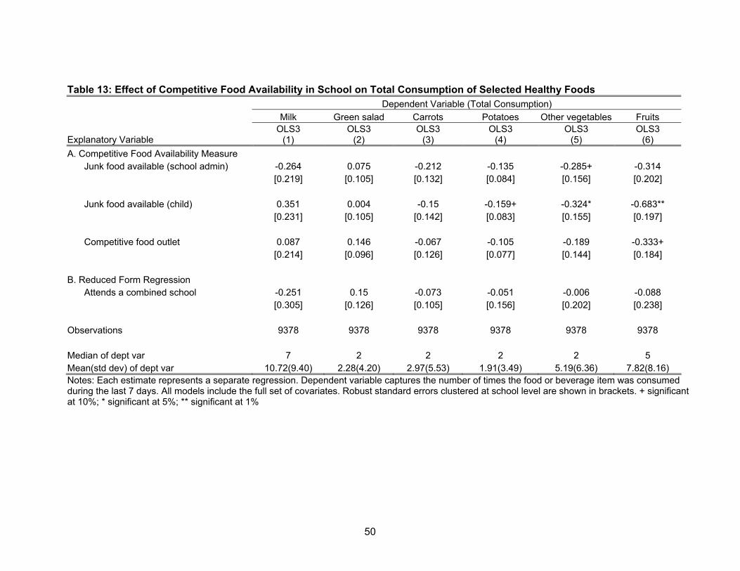
50

Table 13: Effect of Competitive Food Availability in School on Total Consumption of Selected Healthy Foods Dependent Variable (Total Consumption) Milk Green salad Carrots Potatoes Other vegetables Fruits

Explanatory Variable OLS3

(1) OLS3

(2) OLS3

(3) OLS3

(4) OLS3

(5) OLS3

(6) A. Competitive Food Availability Measure

Junk food available (school admin) -0.264 0.075 -0.212 -0.135 -0.285+ -0.314 [0.219] [0.105] [0.132] [0.084] [0.156] [0.202] Junk food available (child) 0.351 0.004 -0.15 -0.159+ -0.324* -0.683** [0.231] [0.105] [0.142] [0.083] [0.155] [0.197] Competitive food outlet 0.087 0.146 -0.067 -0.105 -0.189 -0.333+

[0.214] [0.096] [0.126] [0.077] [0.144] [0.184] B. Reduced Form Regression

Attends a combined school -0.251 0.15 -0.073 -0.051 -0.006 -0.088 [0.305] [0.126] [0.105] [0.156] [0.202] [0.238] Observations 9378 9378 9378 9378 9378 9378 Median of dept var 7 2 2 2 2 5 Mean(std dev) of dept var 10.72(9.40) 2.28(4.20) 2.97(5.53) 1.91(3.49) 5.19(6.36) 7.82(8.16) Notes: Each estimate represents a separate regression. Dependent variable captures the number of times the food or beverage item was consumed during the last 7 days. All models include the full set of covariates. Robust standard errors clustered at school level are shown in brackets. + significant at 10%; * significant at 5%; ** significant at 1%

51

Table 14: Effect of Competitive Food Availability on Children’s Physical Activity in Fifth Grade Dependent Variable

Parent-Reported Days/Week of

Physical Activity Minutes/Week of Physical

Education Instruction in School

OLS3

(1) OLS3

(2) A. Competitive Food Availability Measure

Junk food available (school admin) 0 0.788 [0.050] [1.757] Junk food available (child) -0.02 0.508 [0.047] [1.256] Competitive food outlet -0.005 -0.366

[0.049] [1.502] B. Reduced Form Regression

Attends a combined school 0.120+ 3.013 [0.072] [2.753] Observations 8653 9010 Mean(std dev) of dept var 3.7(1.9) 77.6(31.3) Notes: Each estimate represents a separate regression. All models include the full set of covariates. Robust standard errors clustered at school level are shown in brackets. + significant at 10%; * significant at 5%; ** significant at 1%

52

Table 15: Effect of Competitive Food Availability on Children’s Test Scores and Social-Behavioral Outcomes in Fifth Grade Dependent Variable

Grade 5 Externalizing BP

Score

Grade 5 Internalizing BP

Score

Grade 5 Self-Control/Interpersonal

Skills Score Grade 5

Reading Score Grade 5

Math Score

OLS3

(1) OLS3

(2) OLS3

(3) OLS3

(4) OLS3

(5) A. Competitive Food Availability Measure

Junk food available (school admin) 0.017 -0.001 0.012 0.825 0.264 [0.018] [0.017] [0.021] [0.515] [0.452] Junk food available (child) -0.006 0.004 0.003 2.161** 0.931* [0.016] [0.016] [0.017] [0.474] [0.434] Competitive food outlet -0.007 -0.009 0.004 0.622 0.041

[0.017] [0.017] [0.019] [0.493] [0.442] B. Reduced Form Regression

Attends a combined school 0.060* 0.043 -0.043 0.34 0.511 [0.025] [0.029] [0.026] [0.681] [0.571] Observations 8146 7962 7688 8609 8609 Mean(std dev) of dept var 1.63(0.57) 1.63(0.54) 3.16(0.58) 140(22.7) 114(20.8) Notes: Each estimate represents a separate regression. All models include the full set of covariates. Robust standard errors clustered at school level are shown in brackets. For reading, math, and self control/interpersonal skills, higher scores indicate better outcomes. For externalizing and internalizing behavior problems, higher scores indicate worse outcomes. + significant at 10%; * significant at 5%; ** significant at 1%

53

APPENDIX 1: Effect of Competitive Food Availability on Obesity Status Obese in 5th Grade OLS1 OLS2 OLS3 2SLS1 2SLS2 BVP1 BVP2 (1) Junk food available (school admin) 0.019* 0.009 -0.001 0.004 0.022 -0.031 -0.002 [0.009] [0.010] [0.007] [0.046] [0.037] [0.045] [0.034]

First-stage F-Stat for instruments 22.7 21.56 p-value 0.000 0.000

Overidentification test statistic 0.015 p-value 0.902

(2) Junk food available (child) 0.008 -0.003 -0.001 0.003 0.027 -0.003 -0.003 [0.009] [0.010] [0.008] [0.041] [0.043] [0.041] [0.039]

First-stage F-Stat for instruments 65.96 38.76 p-value 0.000 0.000

Overidentification test statistic 0.002 p-value 0.969

(3) Competitive food outlet 0.025** 0.015 0.008 0.003 0.021 -0.012 0.000 [0.009] [0.009] [0.007] [0.039] [0.034] [0.051] [0.043]

First-stage F-Stat for instruments 28.3 25.79 p-value 0.000 0.000

Overidentification test statistic 0.016 p-value 0.899

Covariates

Child, family & school characteristics Y Y Y Y Y Y Y

State & urbanicity dummies N Y Y Y Y Y Y Baseline BMI N N Y Y Y Y Y

Observations 9378 9378 9378 9378 9378 9378 9378 Notes: All coefficient estimates are marginal effects. Figures in brackets are robust standard errors clustered at the school level. 2SLS1 and BVP1 models use only one instrument (indicator for whether 5th grader is in elementary or combined/middle school) whereas 2SLS2 and BVP2 models use two instruments (highest and lowest grade level in the school).

54

APPENDIX 2: Effect of Competitive Food Availability on Quantiles of BMI Without IV With IV Junk food available (Sch Admin)

10th 0.001 [0.004] 0.011 [0.023] 25th 0.002 [0.004] 0.013 [0.025] 50th -0.001 [0.004] 0.021 [0.028] 75th 0.001 [0.006] 0.036 [0.034] 90th 0.005 [0.007] 0.038 [0.045]

Junk food available (Kid)

10th 0.000 [0.004] 0.005 [0.025] 25th 0.003 [0.003] 0.006 [0.028] 50th 0.000 [0.004] 0.01 [0.033] 75th -0.002 [0.005] 0.01 [0.036] 90th 0.003 [0.007] 0.017 [0.039]

Competitive food outlet

10th -0.001 [0.004] -0.003 [0.021] 25th 0.002 [0.003] -0.002 [0.024] 50th 0.003 [0.004] -0.001 [0.030] 75th 0.010 [0.005] 0.007 [0.038] 90th 0.013 [0.007] 0.009 [0.038]

Observations 9,378 9,378 Notes: Differences in coefficient estimates across quantiles are statistically insignificant in all cases. Figures in brackets are standard errors. Standard errors in quantile regressions without instruments are obtained by bootstrapping and are adjusted for clustering at school level. Standard errors in quantile regressions with instruments are not adjusted for clustering. The estimates and standard errors from IV models are obtained using the Abadie, Angrist, and Imbens (2002) Quantile Treatment Effects (IV-QTE) estimator that is coded in Stata by Froelich and Melly (2008). The IV-QTE regressions include only region fixed effects (versus state fixed effects included in the OLS, 2SLS, and quantile regressions) due to program limitations in Froelich and Melly’s program. However, an alternative IV quantile regression approach using the estimator proposed in Chernozhukov and Hansen (2005) (written in Stata by Le Wang) was also estimated that allowed us to include state fixed effects, and the results were similar. . * significant at 5%; ** significant at 1%.

55

APPENDIX 3: Junk Food Availability Questions in the ECLS-K Fifth Grade Wave

(A). School Administrator Questionnaire:

26. At this school, can students purchase food or beverages from: -

a. One or more vending machines at the school? .................... Yes No

b. A school store, canteen, or snack bar? ................................ Yes No

27. Does this school offer a la carte lunch or breakfast items to students, that is, items not sold as

part of the NSLP School Lunch or the School Breakfast Program?

YES......................................................... 1

NO .......................................................... 2

28. Can students purchase, either from vending machines, school store, canteen, snack bar or a

la carte items from the cafeteria during school hours?

a. Chocolate candy?

b. Other kinds of candy?

c. Cookies, crackers, cakes, pastries, or other baked goods that are not low in fat?

d. Salty snacks that are not low in fat, such as regular potato chips?

e. Ice cream or frozen yogurt that is not low in fat?

f. 2% or whole milk?

g. Fruits or vegetables, not juice?

h. Low-fat cookies, crackers, cakes, pastries, or other low-fat baked goods?

i. Salty snacks that are low in fat, such as pretzels, baked chips, or other low-fat chips?

j. Bread sticks, rolls, bagels, pita bread, or other bread products?

k. Low-fat or fat-free ice cream, frozen yogurt, or sherbet?

l. Low-fat or non-fat yogurt?

m. 1% or skim milk?

56

n. Bottled water?

o. 100% fruit juice?

p. 100% vegetable juice?

q. Soda pop, sports drinks, or fruit drinks that are not 100% juice?

(B). Child Food Consumption Questionnaire:

These questions are about buying food and drinks at your school. Please only think about

buying things at school; do not think about eating at school.

1. In your school, can kids buy {FOOD} in the school?

2. If yes, during the last week that you were in school, how many times did you buy {FOOD} at

school?

a. I did not buy any at school during the last week.

b. 1 or 2 times during the last week in school

c. 3 or 4 times during the last week in school

d. 1 time per day

e. 2 times per day

f. 3 times per day

g. 4 or more times per day

The above set of questions was asked separately for 3 food/beverage groups:

(i) Candy, ice cream, cookies, cakes, brownies or other sweets

(ii) Potato chips, corn chips (Fritos, Doritos), Cheetos, pretzels, popcorn, crackers or other

salty snack foods

57

(iii) Soda pop (EXAMPLES Coke, Pepsi, Mountain Dew), sports drinks (EXAMPLE

Gatorade), or fruit drinks that are not 100% fruit juice (EXAMPLES Kool-Aid, Hi-C,

Fruitopia, Fruitworks)

The next questions ask about food you ate or drank during the past 7 days. Think about all the

meals and snacks you had from the time you got up until you went to bed. Be sure to include food

you ate at home, at school, at restaurants, or anywhere else.

1. During the past 7 days, how many times did you eat/drink {FOOD}?

a. I did not eat/drink {FOOD} during the past 7 days

b. 1 to 3 times during the past 7 days

c. 4 to 6 times during the past 7 days

d. 1 time per day

e. 2 times per day

f. 3 times per day

g. 4 or more times per day

The above question was asked separately for 7 food groups:

1. Milk – Milk question was asked in terms of glasses of milk consumed in last 7 days. This

included all types of milk, including cow’s milk, soy milk or any other kind of milk; includes

the milk {CHILD} drank in a glass or cup, from a carton, or with cereal. The half pint of milk

served at school was counted as one glass.

2. Green salad

3. Potatoes (not counting French fries, fried potato, or potato chips)

4. Carrots

5. Other vegetables

6. Fruits (not counting juice)

58

7. Fast food – meal or snack from a fast food restaurant such as McDonald’s, Pizza Hut,

Burger King, KFC (Kentucky Fried Chicken), Taco Bell, Wendy’s etc.

59

APPENDIX 4: Description of School Outcome Variables

Test Scores: Children surveyed in the ECLS-K were given individually administered math and

reading assessments at each data collection point. In each subject area, assessments consisted

of a two-stage assessment. In the first stage, children received a 12 to 20 item routing test.

Performance on the routing items guided the selection of one of the several alternative second-

stage tests. The second stage test contained items of appropriate difficulty for the level of ability

indicated by the routing test. Since not all children took the exact same test, Item Response

Theory (IRT) scale scores were computed for all children. Reading (math) IRT scores represent

estimates of the number of items students would have answered correctly if they had taken all of

the questions in the first and second stage reading (math) forms. These scores are comparable

across students within a wave and also across waves enabling comparison of children’s

performance over time. The reliability of test scores was very high—0.93 for reading and 0.92 for

math. Touranganeau et al (2006) provides more detailed information about the tests administered.

Social-behavioral outcomes: Measures of children’s social and behavioral outcomes in school

are based on the teacher-reported Social Rating Scale (SRS) administered in each wave of the

ECLS-K. The SRS scale is adapted from the Social Skills Rating System (SSRS) Instrument

developed by Gresham and Elliot (1990), which is a well-established and useful tool in assessing

and targeting social skills deficits and competing problem behaviors. The teacher SRS is a self-

administered questionnaire consisting of two scales externalizing and internalizing behavior

problems. The externalizing scale includes information on acting out behaviors of children and is

based on 5 items that rate the frequency with which a child argues, fights, gets angry, acts

impulsively and disturbs ongoing activities. The internalizing behavior problem scale consists of 4

items that ask about the apparent presence of anxiety, loneliness, low self-esteem, and sadness

in the child. The teacher SRS also includes two scales on positive behaviors such as self-control

60

and interpersonal skills. The self-control scale includes four items that capture the child’s ability to

control behavior by respecting the property rights of others, controlling temper, accepting peer

ideas for group activities, and responding appropriately to pressure from peers. Finally, the

interpersonal skills scale includes five items that rate the child’s skills in forming and maintaining

friendships, getting along with people who are different, comforting or helping other children,

expressing feelings, ideas and opinions in positive ways, and showing sensitivity to the feelings of

others. Teachers use a response scale to report how often the child demonstrated the behavior

described— 1 (never), 2 (occasionally or sometimes), 3 (regularly but not all the time), and 4

(most of the time). The scores on both scales are the mean rating on the items included in the

scale. Higher scores on the externalizing and internalizing scales indicate worse outcomes,

whereas higher scores on the self control and interpersonal skills scales indicate better outcomes.