nebraska transportation centermatc.unl.edu/assets/documents/matcfinal/kim_ndorrese...nebraska...

Nebraska Transportation Center

Report # MPMC-01 Final Report

Research on Roadway Performance and Distress at Low Temperature

Yong-Rak Kim, Ph.D. Associate ProfessorDepartment of Civil EngineeringUniversity of Nebraska-Lincoln

“This report was funded in part through grant[s] from the Federal Highway Administration [and Federal Transit Administration], U.S. Department of Transportation. The views and opinions of the authors [or agency] expressed herein do not necessarily state or reflect those of the U. S. Department of Transportation.”

Nebraska Transportation Center262 WHIT2200 Vine StreetLincoln, NE 68583-0851(402) 472-1975

Soohyok ImGraduate Research AssistantHoki Ban, Ph.D.Postdoctoral Research Associate

26-1121-4004-001

2012


Yong-Rak Kim, Ph.D.

Associate Professor

Department of Civil Engineering

University of Nebraska–Lincoln

Soohyok Im

Graduate Research Assistant



Hoki Ban, Ph.D.

Postdoctoral Research Associate



A Report on Research Sponsored by

Mid-America Transportation Center

University of Nebraska-Lincoln

June 2012

ii

Technical Report Documentation Page 1. Report No

MPMC-01

2. Government Accession

No.

3. Recipient’s Catalog No.

4. Title and Subtitle


5. Report Date

June 2012

6. Performing Organization Code

7. Author/s

Yong-Rak Kim, Soohyok Im, and Hoki Ban

8. Performing Organization Report No.

MPMC-01

9. Performing Organization Name and Address

University of Nebraska-Lincoln


10. Work Unit No. (TRAIS)

362M Whittier Research Center

Lincoln, NE 68583-0856

11. Contract or Grant No.

26-1121-4004-001

12. Sponsoring Organization Name and Address

Nebraska Department of Roads

1500 Hwy. 2

Lincoln, NE 68502

13. Type of Report and Period

Covered

July 2010–June 2012

14. Sponsoring Agency Code

MATC TRB RiP No. 26146

15. Supplementary Notes

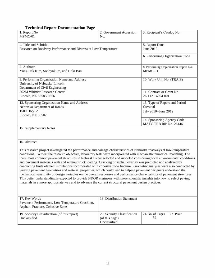
16. Abstract

This research project investigated the performance and damage characteristics of Nebraska roadways at low-temperature

conditions. To meet the research objective, laboratory tests were incorporated with mechanistic numerical modeling. The

three most common pavement structures in Nebraska were selected and modeled considering local environmental conditions

and pavement materials with and without truck loading. Cracking of asphalt overlay was predicted and analyzed by

conducting finite element simulations incorporated with cohesive zone fracture. Parametric analyses were also conducted by

varying pavement geometries and material properties, which could lead to helping pavement designers understand the

mechanical sensitivity of design variables on the overall responses and performance characteristics of pavement structures.

This better understanding is expected to provide NDOR engineers with more scientific insights into how to select paving

materials in a more appropriate way and to advance the current structural pavement design practices.

17. Key Words

Pavement Performance, Low Temperature Cracking,

Asphalt, Fracture, Cohesive Zone

18. Distribution Statement

19. Security Classification (of this report)

Unclassified

20. Security Classification

(of this page)

Unclassified

21. No. of Pages

59 22. Price

iii

Table of Contents

Acknowledgments vi Disclaimer vii

Abstract viii Chapter 1 Introduction 1 1.1. Research Objectives and Scope 2 1.2. Organization of the Report 3 Chapter 2 Background 4

2.1. Mechanism of Thermal Cracking 4 2.2. Modeling of Pavement Structures at Low Temperature 5

Chapter 3 Materials and Laboratory Tests 7 3.1. Materials Selection 7 3.2. Experimental Programs 8 3.2.1. Uniaxial Compressive Cyclic Tests for Linear Viscoelastic

Properties 9 3.2.2. SCB Tests for Fracture Properties 12

Chapter 4 Modeling and Simulation Results 23 4.1. Pavement Geometry and Boundary Condition 23 4.2. Governing Equations for the Model 25

4.3. Layer Properties 28 4.4. Loading 29

4.4.1. Thermal Loading 30

4.4.2. Mechanical Loading 35

4.5. Simulation Results 36 4.5.1. ST1 Simulation with Thermal Loading Only 37

4.5.2. ST2 Simulation with Thermal Loading Only 43 4.5.3. ST3 Simulation with Thermal Loading Only 46 4.5.4. ST1 Simulation with Thermal and Mechanical Loading 52

Chapter 5 Summary and Conclusions 54 5.1. Conclusions 54

Chapter 6 NDOR Implementation Plan 56 References 57

iv

List of Figures

Figure 2.1 Crack propagation in overlay due to temperature changes

(Mukhtar and Dempsey 1996) 4

Figure 3.1 Specimen fabrication and laboratory tests performed for this study 9

Figure 3.2 Uniaxial compressive cycle test results 11

Figure 3.3 SCB test results (force-NMOD) at different loading rates and

temperatures 15

Figure 3.4 Visual observation of SCB specimens after testing 17

Figure 3.5 Schematic illustration of FPZ of typical quasi-brittle materials 18

Figure 3.6 A finite element mesh constructed to model the SCB testing 20

Figure 3.7 SCB test results vs. cohesive model simulation results 22

Figure 4.1 Selected pavement structures: (a) ST1, (b) ST2, and (c) ST3 24

Figure 4.2 Schematic of a finite element model for ST1 25

Figure 4.3 Temporal and spatial temperature variations 31

Figure 4.4 Verification of UTEMP to prescribe temperature field in the

simulations 34

Figure 4.5 Loading and axle configuration of the Class 9 truck used for this study 35

Figure 4.6 Truck loading sequence applied to the pavement simulations 36

Figure 4.7 Horizontal stresses at the surface and at the bottom of the ST1 asphalt

overlay 37

Figure 4.8 Temperature profiles of a 50.8 mm thick asphalt overlay of ST1 38

Figure 4.9 Temperature variations: 101.6 mm vs. 50.8 mm overlay thickness 39

Figure 4.10 Horizontal stresses at the surface and at the bottom of ST1 asphalt

overlay with reduced thickness: 50.8 mm 40

Figure 4.11 Simulation results with engineered material properties 42


overlays 43

Figure 4.13 Simulation results with engineered material properties (ST2) 45


overlays 46

Figure 4.15 Temperature profiles of 50.8-mm thick asphalt overlay of ST3 47

Figure 4.16 Horizontal stresses at the surface and at the bottom of the ST3 asphalt

overlay with reduced thickness: 50.8 mm 48

Figure 4.17 Simulation results with engineered material properties (ST3) 49

Figure 4.18 Simulation results with degraded material properties (ST3) 51

Figure 4.19 Thermo-mechanical pavement response 53

v

List of Tables

Table 3.1 Gradation and properties of aggregates used in this research 8

Table 3.2 Prony series parameters for each different reference temperature 12

Table 3.3 Cohesive zone fracture parameters determined 21

Table 4.1 Material properties of each layer 29

vi

Acknowledgments

The authors thank the Nebraska Department of Roads (NDOR) for the financial support

needed to complete this study. In particular, the authors thank the NDOR Technical Advisory

Committee (TAC) for their technical support and invaluable discussions/comments.

vii

Disclaimer

The contents of this report reflect the views of the authors, who are responsible for the

facts and the accuracy of the information presented herein. This document is disseminated under

the sponsorship of the Department of Transportation University Transportation Centers Program,

in the interest of information exchange. The U.S. Government assumes no liability for the

contents or use thereof.

viii

Abstract

This research project investigated the performance and damage characteristics of

Nebraska roadways at low-temperature conditions. To meet the research objective, laboratory

tests were incorporated with mechanistic numerical modeling. The three most common pavement

structures in Nebraska were selected and modeled considering local environmental conditions

and pavement materials with and without truck loading. Cracking of asphalt overlay was

predicted and analyzed by conducting finite element simulations incorporated with cohesive

zone fracture. Parametric analyses were also conducted by varying pavement geometries and

material properties, which could lead to helping pavement designers understand the mechanical

sensitivity of design variables on the overall responses and performance characteristics of

pavement structures. This better understanding is expected to provide NDOR engineers with

more scientific insights into how to select paving materials in a more appropriate way and to

advance the current structural pavement design practices.

1

Chapter 1 Introduction

Roadway performance and distresses at low temperatures have been overlooked in the

design of pavement mixtures and structures, even though roadway distresses at low-temperature

conditions are the major issues in northern U.S. states. In Nebraska, every year major highways

and local gravel roads are subjected to severe low-temperature conditions, followed by the spring

thaw. In mid-winter, cracks often develop transversely and longitudinally in local gravel roads.

In asphaltic pavements, a number of potholes are created when moisture seeps into the pavement,

freezes, expands, and then thaws. As has been well documented, most potholes are initiated due

to pavement cracks (by fatigue or thermal) and are exacerbated by low temperatures, as water

expands when it freezes to form ice, which results in greater stress on an already cracked road. In

this respect, pavement damage and distresses at low temperatures involve extremely complicated

processes, which cannot be appropriately identified by merely accounting for the thermal

cracking behavior of asphalt binder as the current specifications and pavement design guide

handle.

As an example, for the prediction and characterization of low-temperature cracking

behavior, the current Superpave specifications and the mechanistic-empirical pavement design

guide (MEPDG) are based on the creep and strength data for both asphalt binders and asphalt

mixtures. For asphalt binders, two laboratory instruments were developed during the Strategic

Highway Research Program (SHRP) to investigate the low-temperature behavior of asphalt

binders: the Bending Beam Rheometer (BBR) and the Direct Tension Tester (DTT). For asphalt

mixtures, one laboratory-testing device was developed: the Indirect Tension (IDT) Tester. A

critical temperature is determined at the intersection between the tensile strength-temperature

curve and the thermal stress temperature curve. This approach is used in the thermal cracking

2

(TC) model, which has been implemented in the MEPDG. The TC model has been regarded as a

state-of-the-art tool for performance-based thermal cracking prediction, since the TC model is

based on the theory of viscoelasticity, which mechanically predicts thermal stress as a function

of time and depth in pavements based on pavement temperatures, which are computed using air

temperatures. However, several limitations in the TC model have been identified, such as the use

of the simple, phenomenological crack evolution law to estimate crack growth rate, using test

results obtained from the Superpave IDT test, which does not accurately identify fracture

properties. In addition, the TC model does not consider crack developments related to vehicle

loads and environmental conditions; thus, this model cannot fully reflect fracture processes in the

mixtures and pavements that are subjected to traffic loading, moisture damage, and low-

temperature conditions.

Accordingly, performance and damage characteristics at low-temperature conditions need

to be better understood in relation to structural aspects, materials, and environmental conditions

together, since the issue is not only load related but also is durability associated.

1.1. Research Objectives and Scope

The primary objective of this research was to investigate the performance and damage

characteristics of Nebraska roadways at low-temperature conditions related to the properties of

local paving materials, structural design practices of pavements, and locally observed

environmental conditions. To meet the objective, laboratory tests were incorporated with

mechanistic modeling. Specifically, the three most common pavement structures in Nebraska

were selected and modeled considering local environmental conditions (i.e., time- and depth-

dependent temperature profile) and pavement materials with and without truck loading. The

reflective cracking of the asphalt layer under local conditions was investigated by conducting

3

finite element analyses incorporated with cohesive zone fracture. Parametric analyses were also

conducted by varying pavement geometries and material properties, which would lead to helping

pavement designers understand the mechanical sensitivity of design variables on the overall

responses and performance characteristics of pavement structures. Consequently, this

understanding can better enable engineers to select paving materials in a more appropriate way

and to advance the current materials models and performance models at low-temperature

conditions.

1.2. Organization of the Report

This report is composed of five chapters. Following this introduction, Chapter 2

summarizes the literature reviews for the modeling of pavement considering thermal effects.

Chapter 3 presents the laboratory tests conducted to identify material characteristics at low

temperature, including the dynamic modulus test and fracture test. Chapter 4 describes the finite

element simulations, of the three most common pavement structures, that were conducted. The

simulation results of various cases for parametric analyses are also discussed in the chapter.

Finally, Chapter 5 provides a summary of the findings and conclusions of this study. Future

implementation plans for NDOR are also presented in the chapter.

4

Chapter 2 Background

Many researchers have made great efforts to investigate the thermal cracking behavior of

asphaltic pavement structures. In order to represent the behavior of pavement structures, such as

cracking under thermal loads, it is necessary to examine the thermal cracking mechanism and to

incorporate appropriate constitutive material models into these structural mechanistic models. In

this chapter, various modeling techniques representing the thermal cracking behavior of

pavement structures are described.

2.1. Mechanism of Thermal Cracking

Thermal cracking depends generally on both the magnitude of the low temperature

experienced and the cooling rates. Mukhtar and Dempsey (1996) investigated the thermal

cracking mechanism of the overlay of asphalt concrete (AC) on Portland cement concrete (PCC)

under seasonal temperature changes and daily temperature cycles, as shown in figure 2.1.

Figure 2.1 Crack propagation in overlay due to temperature changes (Mukhtar and Dempsey

1996)

5

As depicted in the figure, they reported that due to the temperature cooling down in the

evening, the temperature on the surface of the slab is cooler than the bottom of the slab because

the effect of the temperature decrease reaches the top of the slab first. The top of the slab

contracts, causing the slab to curl upwards and generating tensile stress in the overlay over the

joint. Potentially, the combination of the PCC slabs and overlay movements due to temperature

differences can cause cracking to initiate from both the top and bottom of the overlay.

2.2. Modeling of Pavement Structures at Low Temperature

Selvadurai et al. (1990) conducted the transient stress analysis of a multilayer pavement

structure subjected to heat conduction and associated thermal-elastic effects by the cooling of its

surface using finite element analysis. They analyzed the pavement structure behavior at low

temperature considering three specific effects: the thickness of the cracked existing asphalt layer,

surface crack depth, and the presence of cracks at both the existing asphalt layer and newly

paved asphalt layers.

The modeling of reflective and thermal cracking of asphalt concrete was conducted using

the cohesive zone model by Dave et al. (2007). Those authors investigated the pavement

behavior of an intermediate climate region located at U.S. State Highway 36 near Cameron,

Missouri. Although they concluded that the finite element simulations with the cohesive zone

model could predict cracking behavior quantitatively, the model validation with field

measurement has not yet been provided for use in the study.

Dave and Buttlar (2010) extended their previous study to investigate the thermal

reflective cracking of asphalt concrete overlays over PCC and rubblized slab considering

different types of mixtures, overlay thickness, and joint spacing of PCC. The authors used the

same modeling technique representing thermal cracking behavior as the previous study, which

6

was cohesive zone fracture modeling. Based on their findings, the overlays over the PCC joints

showed bottom-up cracking, while overlays over rubblized slab revealed top-down cracking.

However, this may not be accurate because the pavement response to the thermal loading may

have been affected by the material properties (i.e., thermal coefficient of asphalt concrete, PCC

slab, and rubblized slab and fracture properties of asphalt concrete) as well as the geometry of

pavement structures.

Kim and Buttlar (2009) examined the low-temperature cracking behavior of airport

pavements under daily temperature change using cohesive zone modeling. To this end, they

performed creep compliance tests, indirect tensile tests (IDT), and disk-shaped compact tension

(DC[T]) tests to obtain numerical model inputs, such as the viscoelastic and fracture properties

of asphalt concrete at low temperature. They reported that two-dimensional fracture models

could successfully simulate the crack initiation and crack propagation. Furthermore, the heavy

aircraft loading, coupled with thermal loading, had an adverse influence on pavement cracking

behavior. However, although the fracture properties are temperature dependent, the fracture

properties of -20oC were used in their models.

Souza and Castro (2012) studied the mechanical response of thermo-viscoelastic

pavements, considering temperature effect. They used an in-house finite element code, which

incorporated the thermo-viscoelastic constitutive model, to investigate the effects of mechanical

tire loading, thermal expansion/contraction, and thermo-susceptibility of viscoelastic asphalt

materials on the overall pavement responses. Through the various sensitivity analyses, they

reported that the deformation and stresses were considerably affected by both thermal

deformation and the thermo-susceptibility of the viscoelastic material, individually and together.

7

Chapter 3 Materials and Laboratory Tests

This chapter presents experimental efforts to characterize the linear viscoelastic and

fracture properties of typical asphaltic paving mixtures subjected to various loading rates at

different low temperatures. To that end, two laboratory tests − uniaxial compressive cyclic tests

to identify the linear viscoelastic properties and semi-circular bending (SCB) fracture tests to

characterize the fracture properties − of a dense-graded asphalt concrete mixture were conducted.

3.1. Materials Selection

For the fabrication and testing of the dense-graded asphalt mixture, three aggregates were

selected and blended: 16 mm limestone, 6.4 mm limestone, and screenings. All three aggregates

were limestone with the same mineralogical origin. The nominal maximum aggregate size

(NMAS) of the final aggregate blend was 12.5 mm. Table 3.1 illustrates gradation, bulk specific

gravity (Gsb), and consensus properties (i.e., fine aggregate angularity (FAA), coarse aggregate

angularity (CAA), and flat and elongated (F&E) particles) of the aggregates used in this study.

The asphalt binder used in this study was Superpave performance graded binder PG 64-28. With

the limestone aggregate blend and the binder, volumetric design of the mixture was performed;

this resulted in a binder content of 6.0% by weight of the total mixture to meet the 4.0% target

air voids and other necessary volumetric requirements.

8

Table 3.1 Gradation and properties of aggregates used in this research

Sieve Analysis (Wash) for Gradation

Aggregate

Sources 19mm 12.7mm 9.5mm #4 #8 #16 #30 #50 #100 #200

16-mm

Limestone 100 95 89 - - - - - - -

6.4-mm

Limestone 100 100 100 72 - - - - - -

Limestone

Screenings 100 100 100 10 3 21 14 10 7 3.5

Combined

Gradation 100 95 89 72 36 21 14 10 7 3.5

Physical and Geometrical Properties

Combined

Properties Gsb = 2.577, FAA(%) = 45.0, CAA(%) = 89.0, F&E(%) = 0

3.2. Experimental Programs

Figure 3.1 briefly illustrates the process of sample fabrication and laboratory tests

performed for this study. Laboratory tests were conducted to obtain linear viscoelastic properties

and to characterize the fracture properties of the mixture. As shown, cylindrical mixture samples

were fabricated using a Superpave gyratory compactor (SGC). Two different specimen

geometries were extracted from the SGC samples. They were (i) cylindrical cores (150 mm in

height and 100 mm in diameter) to be used for determining the linear viscoelastic properties of

the mixture and (ii) semi-circular bending (SCB) specimens (150 mm in diameter and 25 mm

thick with a 2.5 mm-wide and 25 mm-deep mechanical notch) to be used for fracture tests of the

mixture.

9

Uniaxial Compressive Cyclic Test

Semi-circular Bending (SCB) Fracture Test

Uniaxial Compressive Cyclic Test

Semi-circular Bending (SCB) Fracture Test

Figure 3.1 Specimen fabrication and laboratory tests performed for this study

3.2.1. Uniaxial Compressive Cyclic Tests for Linear Viscoelastic Properties

Uniaxial compressive cyclic tests were performed for the linear viscoelastic stiffness of

the mixture. The loading levels were carefully adjusted until the strain levels were within the

range of 0.000050 – 0.000075. Three linear variable differential transformers (LVDTs) were

mounted onto the surface of the specimen at 120o radial intervals with a 100 mm gauge length.

As suggested in the AASHTO TP 62 (2008), five temperatures (-10, 4.4, 21.1, 37.8, and 54.4oC)

and six loading frequencies (25, 10, 5, 1.0, 0.5, and 0.1 Hz) were used, and the frequency-

temperature superposition concept was applied to obtain the linear viscoelastic master curves of

the storage modulus in the frequency domain for a target reference temperature. The testing

results of the storage modulus, as a function of angular frequency, were then fitted with a

mathematical function (i.e., Prony series) based on the generalized Maxwell model as follows:

10

2 2

2 2

1

'( )1

n

i i

ii

EE E

(3.1)

where,

E’(ω) = storage modulus,

ω= angular frequency,

E∞ = long-time equilibrium modulus,

Ei = spring constants in the generalized Maxwell model,

ρi = relaxation time, and

n = number of Maxwell units in the generalized Maxwell model.

Using the Prony series parameters (E∞, Ei, and ρi) obtained by fitting the experimental

data with a storage modulus, the relaxation modulus can be expressed in the time domain as

follows:

1

( ) i

n t

i

i

E t E E e

(3.2)

where,

E(t) = relaxation modulus in time domain, and

t = loading time.

A total of four replicates were tested and the values of the storage modulus at each

different testing temperature, over the range of the loading frequencies, were obtained. Figure

3.2 presents the test results. The test results among the replicates at the same testing conditions

were generally repeatable without large discrepancies.

The test results from replicates were then averaged to produce 30 individual storage

moduli at all levels of temperature and frequency, to produce a stiffness master curve constructed

at a reference temperature. The master curve represents the stiffness of the mixture in a wide

11

range of loading frequencies (or loading times, equivalently). Master curves were constructed

using the time (or frequency) - temperature superposition by shifting data at various

temperatures, with respect to loading frequency, until the curves merged into a single smooth

function. After the shifting was completed, the master curve, at an arbitrary reference

temperature, was then fitted with the Prony series (shown in eq. 3.2) to determine linear

viscoelastic material parameters. Table 3.2 presents Prony series parameters determined for each

different reference temperature. Among them, the Prony series parameters at the reference

temperature of -10oC were used for the low temperature-pavement performance simulation in

Chapter 4.

1.0E+01

1.0E+02

1.0E+03

1.0E+04

1.0E+05

1.0E-08 1.0E-05 1.0E-02 1.0E+01 1.0E+04 1.0E+07

Sto

rag

e M

od

ulu

s (M

Pa)

Reduced Frequency (Hz)

#1 #2 #3 #4 AVG

Figure 3.2 Uniaxial compressive cycle test results

12

Table 3.2 Prony series parameters for each different reference temperature

Reference

Temperature -10

oC 0

oC 21

oC 30

oC

Prony Series

Parameters Ei

(MPa) i

(sec) Ei

(MPa) i

(sec) Ei

(MPa) i

(sec) Ei

(MPa) i

(sec) 1 7391.7 1.0E+00 8095.7 1.0E-01 9095.4 1.0E-05 9028.5 1.0E-05 2 5931.0 1.0E+01 5312.2 1.0E+00 6778.9 1.0E-04 4721.3 1.0E-04 3 6561.0 1.0E+02 4754.5 1.0E+01 7001.4 1.0E-03 4216.1 1.0E-03 4 4526.6 1.0E+03 2243.3 1.0E+02 4250.9 1.0E-02 1879.0 1.0E-02 5 2679.8 1.0E+04 1089.9 1.0E+03 2286.2 1.0E-01 999.9 1.0E-01 6 1238.2 1.0E+05 423.5 1.0E+04 962.4 1.0E+00 397.9 1.0E+00 7 566.9 1.0E+06 203.6 1.0E+05 430.7 1.0E+01 205.7 1.0E+01 8 252.6 1.0E+07 89.8 1.0E+06 186.8 1.0E+02 93.2 1.0E+02 9 124.1 1.0E+08 47.3 1.0E+07 92.8 1.0E+03 52.0 1.0E+03 10 61.0 1.0E+09 23.5 1.0E+08 45.3 1.0E+04 26.2 1.0E+04 11 72.6 1.0E+10 9.1 1.0E+09 53.8 1.0E+05 34.0 1.0E+05 ∞ 236.1 - 323.7 - 215.3 - 229.5 -

3.2.2. SCB Tests for Fracture Properties

To characterize the fracture properties of asphalt mixtures, researchers in the asphaltic

materials and pavement mechanics field have typically pursued four geometries. These are: (i)

single-edge notched beam, SE(B), specimen (Mobasher et al. 1997; Hoare and Hesp 2000;

Marasteanu et al. 2002); (ii) disc-shaped compact tension, DC(T), specimen (Lee et al. 1995;

Wagoner et al. 2005; Wagoner et al. 2006); (iii) semi-circular bending, SCB, specimen

(Molenaar et al. 2002; Li and Marasteanu 2004; van Rooijen and de Bondt 2008; Li and

Marasteanu 2010; Aragao 2011); and (iv) double-edged notched tension, DENT, specimen (Seo

et al. 2002). Among the various options, SCB testing was selected in this study because it has

several benefits compared to other fracture test methods. Even if it has some limitations

(Wagoner et al. 2005), SCB testing is particularly attractive in that it is very repeatable, simple to

perform, and that multiple testing specimens can easily be prepared through a routine process of

mixing and Superpave gyratory compacting of asphalt mixtures. Furthermore, the SCB geometry

is even more attractive considering the fracture characteristics of field cores, which are usually

13

circular. Based on these practical benefits, the SCB testing configuration has become a popular

geometry for evaluating the fracture behavior of bituminous mixtures.

Before testing, individual SCB specimens were placed inside the environmental chamber

of a mechanical testing machine for temperature equilibrium targeting the two different testing

temperatures (-10 and 0oC). Following the temperature conditioning step, specimens were

subjected to a simple three-point bending configuration with four different monotonic

displacement rates (1, 5, 10, and 50 mm/min.) applied to the top center line of the SCB

specimens at each testing temperature. Metallic rollers, separated by a distance of 122 mm (14

mm from the edges of the specimen), were used to support the specimen. Reaction force at the

loading point and vertical crosshead displacements were monitored by the data acquisition

system installed in the mechanical testing machine. A total of 24 SCB specimens were prepared

to complete three replicates per test case of the eight test cases in total (four loading rates at two

different temperatures).

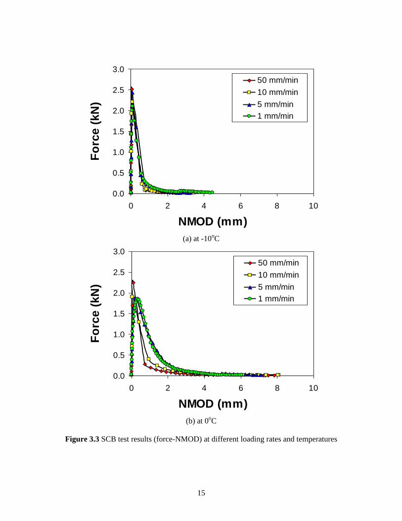
In an attempt to illustrate the effects of testing conditions on the mixture’s fracture

behavior, figure 3.3 presents the SCB test results by plotting the average values between the

reaction forces and opening displacements at different loading rates and different testing

temperatures (i.e., 3.3(a) for -10oC and 3.3(b) for 0

oC). At -10

oC, although the peak force slightly

increases as the loading rate becomes higher, it appears that the fracture behavior is relatively

rate-independent, which is typically observed from a linear elastic fracture state. On the other

hand, asphalt mixture specimens revealed rate-related global mechanical behavior at 0oC. Slower

loading speeds produced more compliant responses than faster cases. Loading rates clearly affect

both the peak force and the material softening, which is represented by the shape of the post-

peak tailing. The trends presented in figure 3.3 suggest that the rate- and temperature-dependent

14

nature of the fracture characteristics needs to be considered when modeling the mechanical

performance of typical asphalt mixtures and pavements with which a wide range of strain rates

and service temperatures is usually associated.

15

0.0

0.5

1.0

1.5

2.0

2.5

3.0

0 2 4 6 8 10

NMOD (mm)

Fo

rce

(k

N)

50 mm/min

10 mm/min

5 mm/min

1 mm/min

(a) at -10

oC

0.0

0.5

1.0

1.5

2.0

2.5

3.0

0 2 4 6 8 10

NMOD (mm)

Fo

rce

(k

N)

50 mm/min

10 mm/min

5 mm/min

1 mm/min

(b) at 0

oC

Figure 3.3 SCB test results (force-NMOD) at different loading rates and temperatures

16

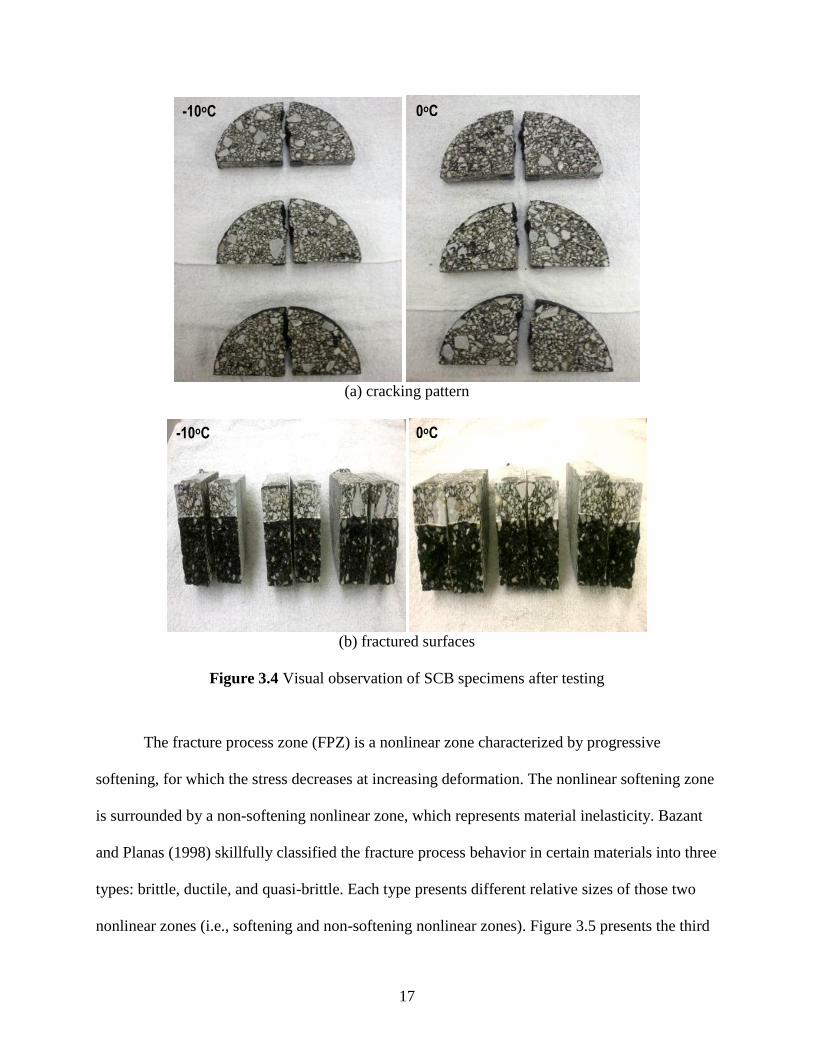
Figure 3.4 presents visual observation of SCB specimens after testing at the two different

temperatures. The cracking pattern is presented in figure 3.4(a), and the fracture surfaces of

individual specimens are shown in figure 3.4(b). It appears that cracks propagated straight from

the crack tip and travelled through the aggregates.

Using SCB test results, the average fracture energy was obtained for each test case. There

were several methods (Wagoner et al. 2005; Marasteanu et al. 2007; Song et al. 2008; Aragao

2011) found in the open literature to calculate the fracture energy. Among them, the finite

element simulations of the SCB tests, with the cohesive zone model, were conducted to

determine the fracture properties that are locally associated to initiate and propagate cracks

through the specimens.

17

(a) cracking pattern

(b) fractured surfaces

Figure 3.4 Visual observation of SCB specimens after testing

The fracture process zone (FPZ) is a nonlinear zone characterized by progressive

softening, for which the stress decreases at increasing deformation. The nonlinear softening zone

is surrounded by a non-softening nonlinear zone, which represents material inelasticity. Bazant

and Planas (1998) skillfully classified the fracture process behavior in certain materials into three

types: brittle, ductile, and quasi-brittle. Each type presents different relative sizes of those two

nonlinear zones (i.e., softening and non-softening nonlinear zones). Figure 3.5 presents the third

-10oC 0oC

-10oC 0oC

18

type of behavior, so-called quasi-brittle fracture. It includes situations in which a major part of

the nonlinear zone undergoes progressive damage with material softening due to microcracking,

void formation, interface breakages, frictional slips, and others. The softening zone is then

surrounded by the inelastic material-yielding zone, which is much smaller than the softening

zone. This behavior includes a relatively large FPZ, as shown in the figure. Asphaltic paving

mixtures are usually classified as quasi-brittle materials (Bazant and Planas 1998; Duan et al.

2006; Kim et al. 2008).

softening

nonlinear hardening

T

tip of FPZtip of physical crack

Tmax

FPZ

c

1.0

T/Tmax

D/c1.0l

Area = Gc

Bilinear Cohesive Zone Model

Figure 3.5 Schematic illustration of FPZ of typical quasi-brittle materials

Cohesive zone models regard fracture as a gradual phenomenon in which separation (Δ)

takes place across an extended crack tip (or cohesive zone) and where fracture is resisted by

cohesive tractions (T). The cohesive zone effectively describes the material resistance when

material elements are being displaced. Equations relating normal and tangential displacement

jumps across the cohesive surfaces with the proper tractions define a cohesive zone model.

Among numerous cohesive zone models developed for different specific purposes, this study

used an intrinsic bilinear cohesive zone model (Geubelle and Baylor 1998; Espinosa and

19

Zavattieri 2003; Song et al. 2006). As shown in figure 3.5, the model assumes that there is a

recoverable linear elastic behavior until the traction (T) reaches a peak value, or cohesive

strength (Tmax), at a corresponding separation in the traction-separation curve. At that point, a

non-dimensional displacement (λ) can be identified and used to adjust the initial slope in the

recoverable linear elastic part of the cohesive law. This capability of the bilinear model to adjust

the initial slope is significant because it can alleviate the artificial compliance inherent to

intrinsic cohesive zone models. The λ value has been determined through a convergence study

designed to find a sufficiently small value to guarantee a level of initial stiffness that renders

insignificant artificial compliance of the cohesive zone model. It was observed that a numerical

convergence could be met when the effective displacement is smaller than 0.0005, which has

been used for simulations in this study. Upon damage initiation, T varies from Tmax to 0, when a

critical displacement (δc) is reached and the faces of the cohesive element are separated fully and

irreversibly. The cohesive zone fracture energy (Gc), which is the locally estimated fracture

toughness, can then be calculated by computing the area below the bilinear traction-separation

curve with peak traction (Tmax) and critical displacement (δc) as follows:

max2

1Tcc G (3.4)

Figure 3.6 presents a finite element mesh, which was finally chosen after conducting a

mesh convergence study. The specimen was discretized using two-dimensional, three-node

triangular elements for the bulk specimen, and zero-thickness cohesive zone elements were

inserted along the center of the mesh to permit mode I crack growth in the simulation of SCB

testing. The Prony series parameters (shown in table 3.2), determined from the uniaxial

20

compressive cyclic tests, were used for the viscoelastic elements, and the bilinear cohesive zone

model illustrated in figure 3.5, was used to simulate fracture in the middle of the SCB specimen

as the opening displacements increased. It should be noted that the simulation conducted herein

involves several limitations at this stage by assuming the mixture as homogeneous and isotropic

with only mode I crack growth, which may not represent the true fracture process of specimens.

cohesive zone elements

150 mm

122 mm

Figure 3.6 A finite element mesh constructed to model the SCB testing

21

The cohesive zone fracture properties (two independent values of the three: Tmax, δc, and

Gc) in the bilinear model were determined for each case through the calibration process until a

good match between test results and numerical simulations was observed. Figure 3.7 presents a

strong agreement between the test results (average of the three SCB specimens) and finite

element simulations. Resulting fracture properties (Tmax and Gc) at each different loading rate and

testing temperature are presented in table 3.3. The good agreement between tests and model

simulations indicates that the local fracture properties were properly defined through the

integrated experimental-numerical approach.

Table 3.3 Cohesive zone fracture parameters determined

Temperature (oC) Loading Rate (mm/min.)

Cohesive Zone Fracture

Parameters

Tmax (kPa) Gc (J/m2)

-10

1 3.2E+03 350

5 3.4E+03 350

10 3.6E+03 350

50 4.0E+03 350

0

1 2.7E+03 750

5 2.7E+03 700

10 3.2E+03 450

50 3.6E+03 400

50 6.5E+02 900

22

0.0

0.5

1.0

1.5

2.0

2.5

3.0

0 2 4 6 8 10

NMOD (mm)

Fo

rce

(k

N)

50 mm/min

10 mm/min

5 mm/min

1 mm/min

Simulation

(a) at -10

oC

0.0

0.5

1.0

1.5

2.0

2.5

3.0

0 2 4 6 8 10

NMOD (mm)

Fo

rce

(k

N)

50 mm/min

10 mm/min

5 mm/min

1 mm/min

Simulation

(b) at 0

oC

Figure 3.7 SCB test results vs. cohesive model simulation results

23

Chapter 4 Modeling and Simulation Results

In this chapter, the three most common asphaltic pavement structures in Nebraska were

modeled through the two-dimensional (2-D) finite element method to investigate the low-

temperature performance of the pavements subjected to thermal and mechanical loading. The 2-

D finite element modeling was conducted by using a commercial package, ABAQUS version 6.8

(2008), with the mechanical material properties as presented in Chapter 3. The ABAQUS

simulation was also incorporated with a user-defined temperature subroutine, UTEMP, to

represent effectively the temporal and spatial temperature profile in the pavement structure. The

reflective cracking of the asphalt layer was simulated for parametric analyses by varying

pavement geometries and layer material properties. This could lead to helping pavement

designers understand the mechanical sensitivity of design variables on the overall responses and

performance characteristics of pavement structures. Consequently, it can enable engineers to

select paving materials in a more appropriate way and to advance the current materials models

and performance models at low-temperature conditions.

4.1. Pavement Geometry and Boundary Condition

Figure 4.1 presents the selected asphaltic pavement structures, ST1, ST2, and ST3, which

are most commonly observed in Nebraska. As can be seen, ST1 (in fig. 4.1 (a)) includes a new

asphalt overlay on a Portland cement concrete (PCC) layer, while ST2 (in fig. 4.1 (b)) and ST3

(in fig. 4.1 (c)) present a new asphalt overlay placed on an existing (old) asphaltic layer. The

base and/or subgrade are then located below the PCC or existing asphalt layer. It is noted that all

three pavement structures have the same asphalt overlay thickness of four inches (101.6 mm).

24

Subgrade

PCC

Base

New AC

101.6 mm

254 mm

152.4mm

101.6 mm

Subgrade

Old AC

Base

New AC

127 mm

50.8 mm

152.4mm

101.6 mm

Subgrade

Old AC

New AC

177.8 mm

152.4mm

101.6 mm

(a) (b) (c)

Figure 4.1 Selected pavement structures: (a) ST1, (b) ST2, and (c) ST3

Among the three pavement structures, figure 4.2 shows a schematic cross-sectional

profile of the ST1 and its details of mesh. All finite element simulations in this study were

conducted in 2-D along the direction of traffic movement. As illustrated, the pavement structure

is repeated with a transverse joint between two PCC slabs. Due to the repeated geometric

characteristics, only the 6,000 mm section, where the PCC joint is located in the middle of the

section, is necessary for the finite element modeling. The asphalt layer is cracked because of

thermal and mechanical loading and the crack is most likely developed from the top of the PCC

joint because of high stress concentration. Therefore, cohesive zone elements are embedded

through the asphalt overlay along the vertical line of the PCC joint for potential cracking due to

thermal effects and/or mechanical truck loading. It can also be noted that the finite element

model is constructed with graded meshes, which can reduce the computational time without

affecting model accuracy. Graded meshes typically have finer elements close to the high-stress

25

gradient zone, such as around the PCC joint in this example and coarser elements for the regions

of low-stress gradient.

101.6 mm

254 mm

152.4mm

101.6 mm

Traffic

6000 mm

6000 mm

AC

PCC

Subgrade

CZ elements

PCC Joint

FC

Figure 4.2 Schematic of a finite element model for ST1

Similarly to the modeling of ST1, it was assumed for the modeling of ST2 and ST3 that

the existing (old) asphalt layer was fully cracked. The cohesive zone elements were also inserted

through the new asphalt overlay along the potential crack path. The same boundary conditions

were applied to all three pavement structures. As illustrated in the figure, both sides of the

vertical edges were fixed in the horizontal direction, and the bottom of the mesh was fixed in the

vertical direction, representing bedrock.

4.2. Governing Equations for the Model

In this study, a thermo-viscoelastic model with cohesive zone fracture was employed for

simulating the fracture behavior of the asphalt layer when the pavement was subjected to varying

low temperatures and mechanical truck loading. In order to avoid unnecessary complexities at

this stage, the inertial effects of the dynamic traffic loads, body forces, and large deformations

were ignored, so the problem could be simplified to quasi-static small strain conditions.

26

It is crucial to select appropriate constitutive models for bulk materials in finite element

modeling. For the modeling of underlying layers (i.e., PCC slab, existing old asphalt layer, base,

and subgrade), linear thermo-elastic behavior is considered. The linear thermo-elastic

constitutive equation can be written as follows:

),(),()(),( txtxxCtx mklmklmijklmij

(4.1)

)(),()(),( m

R

mmklmkl xtxxtx (4.2)

where,

ij = stress tensor,

kl = strain tensor,

)( mijkl xC = elastic modulus tensor,

kl = coefficient of thermal expansion,

),( txm = temperature at a particular position and at a certain time,

)( m

R x = stress-free reference temperature, and

mx = spatial coordinates.

Asphalt concrete material newly placed on top of the PCC slab or an existing old asphalt

layer is modeled as linear, thermorheologically simple, and non-aging viscoelastic, with its

constitutive equation expressed as follows:

27

dx

xdx

xCtx m

mij

mkl

mijklmij

),(),(

),(),(),(

00

(4.3)

)(),(),( mklmijklmij xxCx (4.4)

where,

),( mijkl xC = thermo-viscoelastic relaxation modulus tensor,

),( mij x = second-order tensor of relaxation modulus relating stress to temperature

variations,

= reduced time, and

= time integration variable.

The reduced time can be defined as follows:

t

T

da

t0

))((

1)(

(4.5)

where,

t = real time, and

Ta = temperature shift factor.

The temperature shift factor, ))(( taT , is generally described by either the Arrhenius or

the WLF equations (Williams et al. 1955). In the present study, the shift factor is described

according to the WLF equation:

)(

)(log

2

110 R

R

TC

Ca

(4.6)

where,

21,CC = model constants.

28

The thermo-viscoelastic relaxation modulus of asphalt concrete is determined by

performing laboratory tests, such as dynamic frequency sweep tests, within the theory of linear

viscoelasticity, and test results are mathematically expressed in the form of a Prony series, as

described in Chapter 3. In addition, the cohesive zone model was used to simulate the fracture

process of asphalt surface layers due to thermal-mechanical loading, which was also described in

Chapter 3.

4.3. Layer Properties

Table 4.1 presents the material properties of individual layers for each pavement structure

(ST1, ST2, and ST3). The underlying layers of the pavement structures (i.e., PCC, existing AC,

base, and subgrade) were modeled as isotropic thermo-elastic, while the isotropic thermo-

viscoelastic response with cohesive zone fracture was considered to describe the behavior of the

asphalt concrete surface layer. For simplicity, a Poisson’s ratio of 0.30 was assumed for all

layers. The coefficients of thermal expansion of asphalt mixtures (asphalt overlay and existing

old asphalt) and PCC slab were assumed as 2.5 * 10-5

/oC and 9.9 * 10

-5/oC, respectively. The

interface between each layer was assumed to be fully bonded.

29

Table 4.1 Material properties of each layer

Linear Elastic Properties

Layer E (MPa) v

PCC Slab 26,200

0.30 Existing Asphalt 2,413.2

Base 151.68

Subgrade 43

Linear Viscoelastic Prony Series Parameters (with v = 0.30 and at -10oC of R)

Asphalt Overlay i ρi (sec) Ei (MPa)

1 0.00001 819.3

2 0.0001 1,034.4

3 0.001 1,817.1

4 0.01 2,812.7

5 0.1 4,195.4

6 1.0 5,660.2

7 10 6,614.8

8 100 6,291.0

9 1,000 4,634.1

10 10,000 2,601.5

11 100,000 2,273.9

∞ - 324.8

WLF Model Parameters (at -10oC of R)

Asphalt Overlay C1 = 20.72, C2 = 90.74

Cohesive Zone Fracture Properties

Asphalt Overlay

Temperature Tmax (Pa) Gc (J/m2)

0 3.2 * 105 1,076

-10 3.2 * 105 450

-20 3.2 * 105 330

-30 3.2 * 105 210

Coefficient of Thermal Expansion (/oC)

Asphalt Overlay 2.5 * 10-5

Existing Asphalt 2.5 * 10-5

PCC Slab 9.9 * 10-5

4.4. Loading

This subsection presents two loads (thermal and mechanical) to which the pavement

structure was subjected. Thermal loading was applied to the entire pavement structure based on

the spatial and temporal temperature profile using the user-defined temperature subroutine,

UTEMP, and mechanical loading due to truck tires was applied on the asphalt surface.

30

4.4.1. Thermal Loading

As mentioned earlier, thermal cracks in pavements often occur in a single, critical cooling

event. Thus, prior to performing the thermal cracking simulation, the critical cooling events need

to be researched from historical climate data. Temperature gradients with respect to the

pavement depth for each pavement structure were estimated from the pavement surface

temperature using an enhanced integrated climate model (EICM) developed by AASHTO.

In order to select the critical cooling event for the past 10 years, the historical temperature

data in the city of Lincoln, Nebraska, were researched. According to the temperature data from

1995 to 2005, it was found that the coldest temperature occurred in January of 2005. In that

month, the air temperature dropped down to -22.1oC and the average daily temperature change

was -6oC. Using the EICM, the critical temperature gradients and cooling cycles were estimated

for the three different pavement structures (ST1, ST2, and ST3), as shown in figure 4.3. As

illustrated in the figure, although the surface temperature of each pavement structure is equal, it

varies with pavement depth depending on the underlying layers. In addition, the temperature

variation with respect to time is significant at the surface but it diminishes as the pavement depth

increases.

31

-1200

-800

-400

0

-25 -20 -15 -10 -5 0

De

pth

(m

m)

Temperature (ºC)

6:00 PM

7:00 PM

8:00 PM

9:00 PM

10:00 PM

11:00 PM

00:00 AM

1:00 AM

2:00 AM

3:00 AM

4:00 AM

5:00 AM

(a) pavement ST1

-800

-700

-600

-500

-400

-300

-200

-100

0

-25 -20 -15 -10 -5 0

De

pth

(m

m)

Temperature (ºC)

6:00 PM

7:00 PM

8:00 PM

9:00 PM

10:00 PM

11:00 PM

00:00 AM

1:00 AM

2:00 AM

3:00 AM

4:00 AM

5:00 AM

(b) pavement ST2

Figure 4.3 Temporal and spatial temperature variations

32

-1200

-1000

-800

-600

-400

-200

0

-25 -20 -15 -10 -5 0

De

pth

(m

m)

Temperature (ºC)

6:00 PM

7:00 PM

8:00 PM

9:00 PM

10:00 PM

11:00 PM

00:00 AM

1:00 AM

2:00 AM

3:00 AM

4:00 AM

5:00 AM

(c) pavement ST3

Figure 4.3 Temporal and spatial temperature variations cont’d

Based on the temperature profiles presented in figure 4.3, the time- and depth-dependent

temperature profiles were implemented into the model through the user-defined temperature

module (UTEMP). As observed in the figure, temperature decreases exponentially as depth

increases. Thus, the temperature with depth (T(h)) was presented as an exponential function and

each coefficient was related with time in the form of a fourth-order polynomial, as expressed by

the following set of equations:

4

24

3

23

2

2221202

4

14

3

13

2

1211101

4

04

3

03

2

0201000

210 exp1)(

tAtAtAtAAtA

tAtAtAtAAtA

tAtAtAtAAtA

htAtAtAhT

(4.7)

33

A least-square type error minimization was carried out to obtain the best-fitting model

coefficients, which resulted in a coefficient matrix (3 by 5). A total of 15 coefficients would be

sufficient to model the spatial and temporal temperature variations during the critical cooling

event. For purposes of verification, figure 4.4 compares predicted temperatures from UTEMP to

the actual temperature data of ST1 pavement as an example. It clearly demonstrates that the

temperature approximation by the user subroutine can be successfully used to prescribe the

temperature field in the finite element simulations.

34

Depth (m)

0 2 4 6 8 10 12

Te

mp

era

ture

(o

C)

-18

-16

-14

-12

-10

-8

-6

-4

at 6pm

curve fitting

y=-15.4385+9.8485(1-exp[-5.3807x])

(a) spatial temperature variation at a specific time

y = 0.0027x4 - 0.0551x3 + 0.2224x2 + 0.0738x - 15.5R² = 0.9804

-25

-20

-15

-10

-5

0

0 2 4 6 8 10 12

Te

mp

era

ture

(o

C)

Time (hr)

A0(t)

Regression

(b) temporal temperature variation at a specific location

Figure 4.4 Verification of UTEMP to prescribe temperature field in the simulations

35

4.4.2. Mechanical Loading

Figure 4.5 illustrates the loading configuration of the Class 9 truck used in this study.

Although the truck loading consisted of a front steering axle and two tandem axles with dual

tires, to reduce computational time in the analysis, only the two tandem axles with dual tires

were selected through use of the trapezoidal loading sequence, shown in figure 4.6. A 15.4 m

Class 9 truck trailer traveling at 80 km/h takes 0.692 seconds to pass over a fixed point on the

pavement. Therefore, the first truck passes the fixed point for 0.692 seconds and, after 192

seconds, a second truck passes through the same point. The passage of 450 trucks was simulated

based on the information of the daily maximum amount of truck passes reported by the Nebraska

Department of Road (NDOR).

130 cm 1280 cm

177.8cm

15,400 kg

30.48cm

15,400 kg

130 cm

Figure 4.5 Loading and axle configuration of the Class 9 truck used for this study

36

Figure 4.6 Truck loading sequence applied to the pavement simulations

4.5. Simulation Results

This subsection presents the numerical simulation results of the pavement responses due

to thermal loading only and when the mechanical loading was incorporated with the thermal

loading. Among many mechanical pavement responses, the tensile stresses at the surface and at

the bottom of the asphalt overlay, and the crack opening displacement through the depth of the

asphalt overlay, were examined during the 12 hr cooling event with and without truck loading.

This was because the tensile stresses and the crack opening displacements of the asphalt overlay

are significant indicators to predict cracking and performance behavior of asphaltic pavements at

low-temperature conditions.

Parametric analyses were then conducted by varying pavement geometries and material

properties to better understand the mechanical sensitivity of design variables on the overall

responses and performance characteristics of pavement structures. This understanding can lead to

the selection of paving materials in a more appropriate manner and to the provision of scientific

insights into the more optimized pavement design at low-temperature conditions.

Loading

Time (sec)

0.058 0.634 0.692 192.41 192.47 193.04 193.1

Resting period (450trucks/day)=191.72sec

37

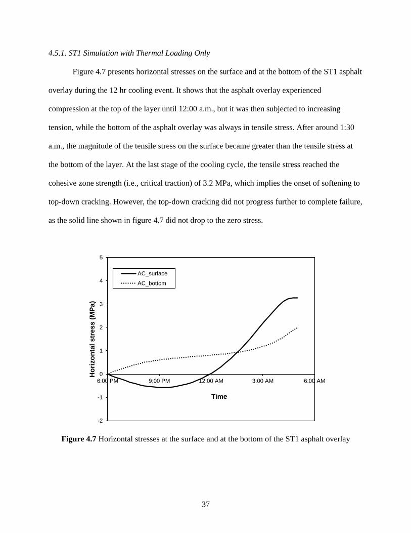
4.5.1. ST1 Simulation with Thermal Loading Only

Figure 4.7 presents horizontal stresses on the surface and at the bottom of the ST1 asphalt

overlay during the 12 hr cooling event. It shows that the asphalt overlay experienced

compression at the top of the layer until 12:00 a.m., but it was then subjected to increasing

tension, while the bottom of the asphalt overlay was always in tensile stress. After around 1:30

a.m., the magnitude of the tensile stress on the surface became greater than the tensile stress at

the bottom of the layer. At the last stage of the cooling cycle, the tensile stress reached the

cohesive zone strength (i.e., critical traction) of 3.2 MPa, which implies the onset of softening to

top-down cracking. However, the top-down cracking did not progress further to complete failure,

as the solid line shown in figure 4.7 did not drop to the zero stress.

-2

-1

0

1

2

3

4

5

6:00 PM 9:00 PM 12:00 AM 3:00 AM 6:00 AM

Ho

rizo

nta

l s

tre

ss

(M

Pa

)

Time

AC_surface

AC_bottom

Figure 4.7 Horizontal stresses at the surface and at the bottom of the ST1 asphalt overlay

38

Based on the simulation results with given default pavement geometry and layer

properties, parametric analyses were attempted by varying asphalt overlay thicknesses and/or

material properties of the asphalt overlay. When the overlay thickness changed, a new

temperature profile was necessary for the simulation because of the overall pavement geometry

change. Figure 4.8 presents a new set of temperature profiles over the pavement depth for the 12

hr cooling cycle, when the asphalt overlay thickness was reduced to 50.8 mm, which is half of

the default thickness of 101.6 mm asphalt overlay.

-800

-400

0

-25 -20 -15 -10 -5 0

De

pth

(m

m)

Temperature (ºC)

6:00 PM

7:00 PM

8:00 PM

9:00 PM

10:00 PM

11:00 PM

00:00 AM

1:00 AM

2:00 AM

3:00 AM

4:00 AM

5:00 AM

Figure 4.8 Temperature profiles of a 50.8 mm thick asphalt overlay of ST1

Figure 4.9 compares temperature variations over the 12 hr cooling cycle at the two

significant locations (surface and bottom of the overlay) when the two different overlay

thicknesses were used. As expected and seen in the figure, the temperature variation between the

two structures is identical at the layer surface, while the lower temperatures and higher variations

39

were observed at the bottom of the asphalt surface layer from the 50.8 mm case. This is because

of the higher insulation of the thicker layer.

Due to the lower temperature and greater temperature susceptibility of the thinner

structure, the 50.8 mm pavement eventually failed, as illustrated in figure 4.10, during the

cooling event. More specifically, the pavement abruptly failed by separation triggered from both

directions at the maximum cooling rate, which is around 4:00 - 5:00 a.m.

-25

-20

-15

-10

-5

0

6:00 PM 9:00 PM 12:00 AM 3:00 AM 6:00 AM

Tem

pera

ture

(o

C)

Time

Temperature variation at 101.6 mm AC_surface

Temperature variation at 50.8 mm AC_surface

Temperature variation at 101.6 mm AC_bottom

Temperature variation at 50.8 mm AC_bottom

101.6 mm

50.8 mm

Figure 4.9 Temperature variations: 101.6 mm vs. 50.8 mm overlay thickness

40

-2

-1

0

1

2

3

4

5

6:00 PM 9:00 PM 12:00 AM 3:00 AM 6:00 AM

Ho

rizo

nta

l s

tre

ss

(M

Pa

)

Time

AC_surface

AC_bottom

Figure 4.10 Horizontal stresses at the surface and at the bottom of ST1 asphalt overlay with

reduced thickness: 50.8 mm

In an attempt to investigate the effects of engineered properties of paving materials on

performance behavior, two other simulations were conducted by varying two different categories

of layer properties: the coefficient of thermal expansion and the fracture property of the asphalt

overlay. According to a study by Mamlouk et al. (2005), the coefficient of thermal expansion of

asphalt concrete mixtures typically ranges from 1.1 * 10-5

/oC to 3.71 * 10

-5/oC. Thus, in this

study, the lowest bound value (i.e., 1.1 * 10-5

/oC) was tried and compared to the case with the

default value (i.e., 2.5 * 10-5

/oC) to examine to what degree cracking resistance of the pavement

can be improved due to the engineered material property. Regarding the effects of fracture

property, a 30% increase of the default cohesive zone strength (Tmax) was used. For all the cases,

the simulation result in figure 4.10 was compared as a reference case. Figures 4.11(a) and (b)

present the simulation results. As shown in the figures, pavements with engineered properties

could last during the cooling cycle without fracture. The simulation results shown in figure

41

4.11(a) indicate that the lower coefficient of thermal expansion could significantly reduce the

tensile stress at the asphalt surface, although it did not change tensile stresses at the bottom of the

asphalt overlay. When the asphalt overlay was more crack resistant with the increased cohesive

zone strength, as illustrated in figure 4.11(b), the pavement did not show thermal cracking, since

the resulting tensile stress was lower than the critical stress state causing material separation.

From the simulation results shown herein, it can be concluded that the engineered paving

materials can significantly contribute to the reduction of pavement thickness, which could lead to

much more economic and optimized pavement structural design.

42

-2

-1

0

1

2

3

4

5

6:00 PM 9:00 PM 12:00 AM 3:00 AM 6:00 AM

Ho

rizo

nta

l s

tre

ss

(M

Pa

)

Time

AC_surface when a=2.50E-5

AC_bottom when a=2.50E-5



(a) α = 2.5 * 10

-5/oC vs. 1.1 * 10

-5/oC

-2

-1

0

1

2

3

4

5

6:00 PM 9:00 PM 12:00 AM 3:00 AM 6:00 AM

Ho

rizo

nta

l s

tre

ss

(M

Pa

)

Time

AC_surface when Tmax=3.20

AC_bottom when Tmax=3.20



(b) Tmax = 3.2 MPa vs. Tmax = 4.16 MPa

Figure 4.11 Simulation results with engineered material properties

43


Figure 4.12 presents horizontal stresses on the surface and at the bottom of the ST2

asphalt overlay during the 12 hr cooling event. Similar to the results of the ST1 structure, the

asphalt overlay experienced compression at the top of the layer for about six hours, and then it

was subjected to increasing tension until it met the softening threshold. The horizontal stress at

the bottom of the asphalt overlay is, however, mostly under a tensile state. At around 2:00 a.m.,

the magnitude of tensile stress on the overlay surface reached the cohesive strength (3.2 MPa),

which triggered the progressive material softening, followed by fracture. Top-down cracking

occurred, as the figure shows zero traction on the surface of asphalt overlay at the end of the

simulation.

-4

-3

-2

-1

0

1

2

3

4

5

6:00 PM 9:00 PM 12:00 AM 3:00 AM 6:00 AM

Ho

rizo

nta

l s

tre

ss

(M

Pa

)

Time

AC_surface

AC_bottom

Figure 4.12 Horizontal stresses at the surface and at the bottom of ST2 asphalt overlay

44

Since the top-down thermal cracking was expected in the ST2 pavement when it was

designed with the default values of layer thickness and measured values of material properties,

some design alternatives could be considered to improve pavement performance at low-

temperature conditions. Better pavement performance can be achieved by either increasing the

overlay thickness or replacing the current materials with engineered ones. Figure 4.13 presents

simulation results when the asphalt overlay material has been modified to represent lower

temperature susceptibility (i.e., a lower value of the coefficient of thermal expansion) or greater

fracture resistance with an improved cohesive strength by 30%. In both cases, the ST2 pavement

did not fail due to the thermal cracking, even though it experienced a softening process. Clearly,

engineered paving materials allow the pavement structure to perform better by being able to

sustain the damage and avoid failure.

45

-4

-3

-2

-1

0

1

2

3

4

5

6:00 PM 9:00 PM 12:00 AM 3:00 AM 6:00 AM

Ho

rizo

nta

l s

tre

ss

(M

Pa

)

Time





(a) α = 2.5 * 10

-5/oC vs. 1.1 * 10

-5/oC

-4

-3

-2

-1

0

1

2

3

4

5

6:00 PM 9:00 PM 12:00 AM 3:00 AM 6:00 AM

Ho

rizo

nta

l s

tres

s (

MP

a)

Time






Figure 4.13 Simulation results with engineered material properties (ST2)

46


Simulation results of horizontal stresses on the surface and at the bottom of the ST3

pavement are presented in figure 4.14. In comparison with the results of the ST2 pavement, ST3

sustained no cracking through the 12 hr cooling cycle. At the top of the layer, the asphalt overlay

was in compression for six hours, and then was subjected to increasing tension, while the

horizontal stress at the bottom of the layer was completely in tension. The overlay surface met

the softening threshold at around 2:00 a.m., which implies the onset of top-down damage

(material softening). However, thermal cracking did not occur as the figure shows residual

resistance of the layer at the end of the cooling cycle.

-4

-3

-2

-1

0

1

2

3

4

5

6:00 PM 9:00 PM 12:00 AM 3:00 AM 6:00 AM

Ho

rizo

nta

l s

tres

s (

MP

a)

Time

AC_surface

AC_bottom

Figure 4.14 Horizontal stresses at the surface and at the bottom of ST3 asphalt overlay

47

Based on the simulation results from the default pavement geometry and the layer

properties of ST3, several additional simulations were attempted. Figure 4.15 presents a new set

of temperature profiles over the pavement depth to conduct model simulations with the reduced

thickness of asphalt overlay to 50.8 mm, and figure 4.16 shows simulation results plotting

horizontal stresses at the two critical locations (top and bottom of the asphalt overlay) over time.

-1200

-1000

-800

-600

-400

-200

0

-25 -20 -15 -10 -5 0

De

pth

(m

m)

Temperature (ºC)

6:00 PM

7:00 PM

8:00 PM

9:00 PM

10:00 PM

11:00 PM

00:00 AM

1:00 AM

2:00 AM

3:00 AM

4:00 AM

5:00 AM

Figure 4.15 Temperature profiles of 50.8 mm thick asphalt overlay of ST3

As presented in figure 4.16, the tensile stresses both at the surface and at the bottom of

the asphalt overlay reached the critical traction around 8 hrs into the cooling cycle and eventually

dropped down to zero, implying that the pavement layer fully cracked due to the thermal loading.

This was an expected result since the thinner overlay presents higher gradients of thermal strain,

which corresponds to greater thermal cracking susceptibility than the thicker layer.

48

-4

-3

-2

-1

0

1

2

3

4

5

6:00 PM 9:00 PM 12:00 AM 3:00 AM 6:00 AM

Ho

rizo

nta

l s

tres

s (

MP

a)

Time

AC_surface

AC_bottom

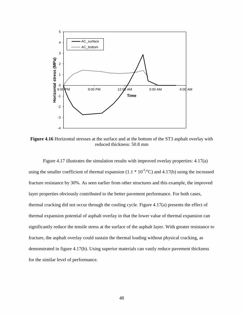
Figure 4.16 Horizontal stresses at the surface and at the bottom of the ST3 asphalt overlay with

reduced thickness: 50.8 mm

Figure 4.17 illustrates the simulation results with improved overlay properties: 4.17(a)

using the smaller coefficient of thermal expansion (1.1 * 10-5

/oC) and 4.17(b) using the increased

fracture resistance by 30%. As seen earlier from other structures and this example, the improved

layer properties obviously contributed to the better pavement performance. For both cases,

thermal cracking did not occur through the cooling cycle. Figure 4.17(a) presents the effect of

thermal expansion potential of asphalt overlay in that the lower value of thermal expansion can

significantly reduce the tensile stress at the surface of the asphalt layer. With greater resistance to

fracture, the asphalt overlay could sustain the thermal loading without physical cracking, as

demonstrated in figure 4.17(b). Using superior materials can vastly reduce pavement thickness

for the similar level of performance.

49

-5

-4

-3

-2

-1

0

1

2

3

4

5

6:00 PM 9:00 PM 12:00 AM 3:00 AM 6:00 AM

Ho

rizo

nta

l s

tre

ss

(M

Pa

)

Time





(a) α = 2.5 * 10

-5/oC vs. 1.1 * 10

-5/oC

-5

-4

-3

-2

-1

0

1

2

3

4

5

6:00 PM 9:00 PM 12:00 AM 3:00 AM 6:00 AM

Ho

rizo

nta

l s

tre

ss

(M

Pa

)

Time






Figure 4.17 Simulation results with engineered material properties (ST3)

50

Another set of simulations was also attempted by applying poorer materials to the

reference pavement geometry of 101.6 mm thick asphalt overlay. Based on the study by

Mamlouk et al. (2005), who presented the typical range of value from 1.1 * 10-5

/oC to 3.71 *

10-5

/oC, the highest bound value (i.e., 3.71 * 10

-5/oC) was tried and compared to the case with the

default value (i.e., 2.5 * 10-5

/oC) to examine how much the cracking resistance of the pavement

would be reduced. Regarding the effects of fracture property, a 30% decrease of the default

cohesive zone strength was used. As illustrated in figure 4.18, the ST3 pavement fully cracked in

both cases. Inferior materials clearly induced more damage and premature failure of the

structure. Simulation results herein and earlier indicate that the performance-based pavement

design can be achieved by mechanistic analyses of the pavement structure based on the

fundamental properties of the layer materials.

51

-5

-4

-3

-2

-1

0

1

2

3

4

5

6:00 PM 9:00 PM 12:00 AM 3:00 AM 6:00 AM

Ho

rizo

nta

l s

tre

ss

(M

Pa

)

Time





(a) = 2.5 * 10

-5/oC vs. 3.71 * 10

-5/oC

-5

-4

-3

-2

-1

0

1

2

3

4

5

6:00 PM 9:00 PM 12:00 AM 3:00 AM 6:00 AM

Ho

rizo

nta

l s

tre

ss

(M

Pa

)

Time






Figure 4.18 Simulation results with degraded material properties (ST3)

52

4.5.4. ST1 Simulation with Thermal and Mechanical Loading

Although it has been known that pavement cracks often occur in a single, critical cooling

event at low-temperature conditions, the effects of heavy vehicles on pavement damage also

need to be investigated since the pavement, in reality, is subjected to the truck loads and low

temperatures simultaneously. To that end, thermo-mechanical model simulations were also

conducted in this research. For the simulation, the ST1 pavement with its default pavement

geometry and material properties was selected, and the Class 9 truck trailer illustrated in figure

4.5 was applied to the pavement to represent vehicles traveling at 80 km/h for a total of 450

passages. To represent critical traffic loading conditions, the truck tire loading was placed right

above the cohesive zone elements.

As in other simulations with thermal loading only, the horizontal stresses and cohesive

zone opening displacements over the depth of asphalt overlay were monitored. Simulation results

were then compared to the results from the reference case in order to examine the effects of

mechanical loading on the pavement performance at low-temperature conditions. Figure 4.19

presents the model simulation results plotting the cohesive zone opening displacements within

the asphalt overlay, at the end of the cooling cycle (i.e., 5:00 a.m.) and truck passing (i.e., 450

passes). As shown in the figure, no huge discrepancy was observed in the cohesive zone opening

displacement between the two cases. This implies that the mechanical truck loading does not

affect pavement damage and failure significantly at low-temperature conditions, which

subsequently infers that the truck loading could be ignored for the structural design of pavements

associated with low temperatures.

53

-120

-100

-80

-60

-40

-20

0

0 0.002 0.004 0.006 0.008 0.01

Dep

th f

rom

th

e s

urf

ace (

mm

)

Crack opening displacement (mm)

Thermal loading

Thermal + Mechanical loading

Figure 4.19 Thermo-mechanical pavement response

54

Chapter 5 Summary and Conclusions

This research project investigated the performance and damage characteristics of

Nebraska roadways at low-temperature conditions. To meet the research objective, laboratory

tests were incorporated with mechanistic numerical modeling. Three of the most common

pavement structures in Nebraska were selected and modeled considering local environmental

conditions and pavement materials, with and without truck loading. Cracking of asphalt overlay

was predicted and analyzed by conducting finite element simulations incorporated with a user-

defined temperature subroutine and cohesive zone fracture. Parametric analyses were also

conducted by varying pavement geometries and material properties, which could lead to helping

pavement designers understand the mechanical sensitivity of design variables on the overall

responses and performance characteristics of pavement structures. This better understanding is

expected to provide NDOR engineers with more scientific insights for the selection of paving

materials in a more appropriate way and to advance the current structural pavement design

practices. Based on the test and simulation results, the following conclusions were drawn.

5.1. Conclusions

Two-dimensional finite element simulation was successfully conducted for predicting

the thermo-mechanical performance of typical asphaltic pavement structures in

Nebraska. The finite element modeling was integrated with experimental tests to

investigate the fracture process (initiation and propagation of cracks) of asphaltic

pavements due to thermal and/or mechanical loading.

Nonlinear temperature gradients, which are time dependent and spatially variant, were

effectively implemented into the finite element modeling by using the national climate

data, the enhanced integrated climate model (EICM), and the user-defined temperature

55

module (UTEMP), which was developed for this research. Model simulations were

conducted by projecting the nonlinear temperature data into the finite element mesh for

the coldest 12 hr cooling cycle (6:00 p.m. to 5:00 a.m.) in hourly time steps.

All pavement structures examined in this project presented sensitive mechanical

responses due to the thermal loading. In addition, pavement responses were

significantly affected by variation of pavement geometry and layer material properties,

such as the coefficient of thermal expansion and fracture characteristics. Engineered

paving materials, such as the one with 30% improved fracture resistance, could reduce

surface layer thickness by 50% to meet the similar low-temperature performance.

The effects of heavy vehicles on the pavement damage at low-temperature conditions

were investigated by applying thermal loading and mechanical truck loading

simultaneously. This thermo-mechanical finite element simulation demonstrated that no

huge discrepancy in the cohesive zone opening displacement occurred compared to the

case with thermal loading only. This implies that the mechanical truck loading does not

affect pavement damage and failure significantly at low-temperature conditions, which

subsequently implied that the truck loading could be ignored for the structural design of

pavements associated with low temperatures.

The mechanistic approach based on fundamental theories and material characteristics

seems very reasonable and useful to better aid in the selection of paving materials and

to enable performance-based pavement design. Nevertheless, field validation is

necessary to prove the benefits and accuracy of the finite element pavement modeling.

Therefore, it is recommended to continue this effort for advancing the current pavement

design concept, which will be more and more mechanistic in the future.

56

Chapter 6 NDOR Implementation Plan

NDOR plans on expanding the SCB test to production on actual projects during

construction to gather their SCB strengths and correlating them to field performance in an effort

to guide potential future designs for thickness, and support same and better low temperature

crack resistant leveling courses, base layers and surface layers. This will support the thin lift

strategies that are becoming so important and vital to Nebraska’s and the nation’s resurfacing

strategies.

57

References

AASHTO TP 62-07. 2008. “Determining dynamic modulus of hot-mix asphalt concrete

mixtures.” Standard Specifications for Transportation and Methods of Sampling and

Testing, 28th Edition, and Provisional Standards. America Association of State

Transportation and Highway Engineering.

ABAQUS. 2008. “Version 6.8.” Hibbt, Karlsson, and Sorenson, Inc.: Pawtucket, Rhode Island.

Aragão, F. T. S. 2011. “Computational microstructure modeling of asphalt mixtures subjected to

rate-dependent fracture.” Ph.D. Dissertation, University of Nebraska, Lincoln.

Bazant, Z. P. and J. Planas. 1998. Fracture and size effect in concrete and other quasibrittle

materials. Boca Raton, FL: CRC Press LLC.

Dave, E. V., S. H. Song, W. G. Buttlar, and G. H. Paulino. 2007. “ Reflective and thermal

cracking modeling of asphalt concrete.” Proceedings of the Advanced Characterization

of Pavement and Soil Engineering Materials, Athens, Greece, 1241-1252

Dave, E. V. and W. G. Buttlar. 2010. “Thermal reflective cracking of asphalt concrete overlays.”

International Journal of Pavement Engineering 11, no. 6: 477-488.

Duan, K., X. Hu, and F. H. Wittmann. 2006. “Scaling of quasi-brittle fracture: boundary and size

effect.” Mechanics of Materials 38: 128-141.

Espinosa, H. D. and P. D. Zavattieri. 2003. “A grain level model for the study of failure initiation

and evolution in polycrystalline brittle materials, part I: theory and numerical

implementation.” Mechanics of Materials 35: 333-364.

Geubelle, P. and J. Baylor. 1998. “Impact-induced delamination of laminated composites: a 2D

simulation.” Composites Part B – Engineering 29, no. 5: 589-602.

Hoare, T. R. and S. Hesp. 2000. “Low-temperature fracture testing of asphalt binders: regular

and modified systems.” Transportation Research Record 1728: 36-42.

Kim, H., M. P. Wagoner, and W. G. Buttlar. 2008. “Simulation of fracture behavior in asphalt

concrete using a heterogeneous cohesive zone discrete element model.” Journal of

Materials in Civil Engineering 20, no. 8: 552-563.

Kim, H. and W. G. Buttlar. 2009. “Finite element cohesive fracture modeling of airport

pavements at low temperatures.” Cold Regions Science and Technology 57: 123-130.

Lee, N. K., G. R. Morrison, and S. Hesp. 1995. “Low temperature fracture of poluethylene-

modified asphalt binders and asphalt concrete mixes.” Journal of the Association of

Asphalt Paving Technologists 64: 534-574.

58

Li, X. and M. O. Marasteanu. 2004. “Evaluation of the low temperature fracture resistance of

asphalt mixtures using the semi-circular bend test.” Journal of the Association of Asphalt

Paving Technologists 73: 401-426.

Li, X. and M. O. Marasteanu. 2010. “The fracture process zone in asphalt mixture at low

temperature.” Engineering Fracture Mechanics 77: 1175-1190.

Mamlouk, M. S., M. W. Witczak, K. E. Kaloush, and N. Hasan. 2005. “Determination of thermal

properties of asphalt mixtures.” Journal of Testing and Evaluation 33, no. 2: 1-9.

Marasteanu, M. O., S. T. Dai, J. F. Labuz, and X. Li. 2002. “Determining the low-temperature

fracture toughness of asphalt mixtures.” Transportation Research Record 1789: 191-199.

Marasteanu, M. O., A. Zofka, M. Turos, X. Li, R. Velasques, W. Buttlar, G. Paulino, A. Braham,

E. Dave, J. Ojo, H. Bahia, C. Williams, J. Bausano, A. Gallistel, and L. McGraw. 2007.

“Investigation of low temperature cracking in asphalt pavements: national pooled fund

study 776.” Final Report No. MN/RC 2007-43, Minnesota Department of Transportation.

Mobasher, B., M. S. Mamlouk, and H. M. Lin. 1997. “Evaluation of crack propagation properties

of asphalt mixtures.” Journal of Transportation Engineering, 123, no. 5: 405-413.

Molenaar, A. A. A., A. Scarpas, X. Liu, and S. M. J. G. Erkens. 2002. “Semicircular bending

test: simple but useful?” Journal of the Association of Asphalt Paving Technologists, 71:

794-815.

Mukhtar, M. T. and B. J. Dempsey. 1996. “Interlayer stress absorbing composite (ISAC) for

mitigating reflective cracking in asphalt concrete overlays.” Final Report, Transportation

Engineering Series No. 94, Cooperative Highway and Transportation Series No. 260,

University of Illinois, Urbana, IL.

Seo, Y., Y. R. Kim, and M. W. Witczak. 2002. “Application of the digital image correlation

method to mechanical testing of asphalt-aggregate mixtures.” Transportation Research

Record 1789: 162-172.

Slevadurai, A. P. S., M. C. Au, and W. A. Phang. 1990. “Modeling of low-temperature behavior

of cracks in asphalt pavement structures.” Canadian Journal of Civil Engineering, 17:

844-858.

Song, S. H., G. H. Paulino, and W. G. Buttlar. 2006. “A bilinear cohesive zone model tailored

for fracture of asphalt concrete considering viscoelastic bulk material.” Engineering

Fracture Mechanics, 2829-2847.

Song, S. H., M. P. Wagoner, and G. H. Paulino. 2008. “δ25 crack opening displacement

parameter in cohesive zone models: experiments and simulations in asphalt concrete.”

Fatigue and Fracture of Engineering Materials and Structures, 31: 850-856.

59

Souza, F. V. and L. S. Castro. 2012. “Effect of temperature on the mechanical response of

thermo-viscoelastic asphalt pavements.” Construction and Building Materials, vol. 30:

574-582.

van Rooijen, R. C. and A. H. de Bondt. 2008. “Crack propagation performance evaluation of

asphaltic mixes using a new procedure based on cyclic semi-circular bending tests.”

Pavement cracking: mechanisms, modeling, detection, testing, and case histories, CRC

Press, 437-446.

Wagoner, M. P., W. G. Buttlar, and G. H. Paulino. 2005. “Disk-shaped compact tension test for

asphalt concrete fracture.” Society for Experimental Mechanics, 45, no. 3: 270-277.

Wagoner, M. P., W. G. Buttlar, G. H. Paulino, and P. Blankenship. 2006. “Laboratory testing

suite for characterization of asphalt concrete mixtures obtained from field cores.” Journal

of the Association of Asphalt Paving Technologists, 75: 815-852.

Williams, M. L., R. F. Landel, and J. D. Ferry. 1955. “The temperature dependence of relaxation

mechanisms in amorphous polymers and other glass-forming liquids.” Temperature

Dependence of Relaxation Mechanisms, 3701-3707.

nebraska transportation centermatc.unl.edu/assets/documents/matcfinal/kim_ndorrese...nebraska...

Documents