network externalities in supermarket retailingshamilto/papers/network_ext_paper_4_08.pdfrecognizing...

Authors are Marvin and June Morrison Chair of Agribusiness, Morrison School of*

Management and Agribusiness, Arizona State University, Mesa, AZ; Assistant Professor in theDepartment of Advertising, Public Relations and Retailing, Michigan State University, EastLansing, MI; and Professor, Orfalea School of Business, California Polytechnic State University,San Luis Obispo, CA. Contact author: Richards. email: [email protected]. Copyright 2007. Allrights reserved. Do not copy or cite without permission.

Network Externalities in Supermarket Retailing

Timothy J. Richards, Geoff Pofahl, and Stephen F. Hamilton*

mailto:[email protected].

1

Introduction

In the 1990s and early 2000s, retail consolidation and the expansion of “big box” retailers in the

food industry changed the way consumers buy food in most urban markets (Martinez). Most

explanations for this phenomenon focused on scale economies and supply chain efficiencies

achieved by retailers such as Wal Mart and Target in the U.S. and Tesco and Carrefour abroad.

However, empirical estimates of production-side scale economies in food retailing are small,

likely too small to generate the type of industry dominance now in place (Cotterill, 1986).

Rather, we argue that much of the advantage is likely due to demand-side scale economies, in

particular, to a form of indirect network effect generated by a two-sided demand for retail shelf

space.

Retailers are platforms that exist only to connect consumers and manufacturers.

Consumers prefer a variety of products, so value platforms that are able to attract a larger number

of manufacturers. On the other side, manufacturers benefit by selling through a platform that is

able to attract the greatest number of consumers. Both consumers and manufacturers pay a price

for access – the retail price for consumers, and either access fees (slotting fees, promotional

allowances, etc.) or comparatively low wholesale prices for retailers who do not charge slotting

(Hamilton, 2004; Rao, 2004). In this study, we describe a general model wherein retail

supermarkets serve as platforms in a two-sided market that consists of consumers on one side

and manufacturers on the other. Because consumers are assumed to demand variety (Draganska

and Jain, 2005; Richards and Hamilton, 2006) and manufacturers prefer more shelf-space, the

price retailers charge to both sides must take the demand from the other into account.

Recognizing the two-sided nature of retail markets explains many of the trends toward

2

consolidation and off-invoice pricing activity, or lack thereof, in the supermarket industry over

the last decade.

Many technology markets exhibit network externalities. Telecommunications (Rochet

and Tirole, 2002, 2003), spreadsheet software (Church and Gandal, 1992) and personal digital

assistants (Nair, Chintagunta, Dube, 2004) are but a few examples. In each of these cases, the

demand for the underlying technology increases the more users have purchased either the

technology itself, or related software. It is well understood that network externalities have

significant impacts for product pricing, given the importance of becoming established as the

standard technology (Katz and Shapiro, 1984; Farrell and Saloner, 1992). Other markets exhibit

a similar type of network externality that depends not upon the mutual dependence of hardware

and software, but the two-sided nature of the market. For example, Rysman (2004) and Kaiser

and Wright (2006) show that advertisers’ demand for space depends upon the number of readers

that will see the ad, and reader demand depends upon the number of advertisers that choose a

particular platform (yellow pages, or magazine, respectively). This study is the first to

empirically estimate the extent of indirect network effects in food retailing.

Our model follows Armstrong (2006) and Kaiser and Wright (2006) in that we adopt a

general model of retail pricing under two-sided demand and network externalities. In our model,

the network effects arise from a demand for variety from consumers and a demand for

distribution by manufacturers. Consumer demand is hierarchical as consumers choose from

among available stores based on average prices and assortment depth, and purchase quantities

based on price. Store choice is represented by a discrete-choice Hotelling (1929) model and

purchase quantities with a general CES model. By aggregating all data to the category-level, our

3

model represents a new way to consider retail demand for the entire “shopping-basket.”

The objective of this paper is to determine whether pricing and assortment behavior by

retailers, both upstream with respect to manufacturers and downstream with respect to

consumers, is consistent with a two-sided demand environment. And if it is, we aim to describe

the nature of retailers’ behavior and compare it to other industries where network effects are

more common and well understood. In estimating the upstream pricing behavior of supermarket

retailers, we also contribute to the retailing literature in that we develop a method for inferring

the price of shelf space, or slotting fees in more usual terminology.

In the first section, we develop an economic model of two-sided demand in the retail

supermarket industry. An econometric model is developed in the second section that is able to

test the implications of network pricing by retailers. This model consists of both downstream

(consumer) and upstream (manufacturer) components. We describe our data and estimation

methods in the third section, and present the results in a fourth. A concluding section offers

some implications both for supermarket retailing strategy and as a potential explanation for

emerging trends in the industry.

Economic Model of Supermarket Retailers as Two-Sided Demand Platforms

The theoretical literature on pricing in markets with two-sided demand is very rich as there are a

number of examples, each subtly different from the other. Katz and Shapiro (1985), Rochet and

Tirole (2002, 2003), Armstrong (2006) presents the general case for a multi-retailer platform and

an advertising platform such as a magazine or yellow pages. In a two-firm Hotelling-type

4

framework, Armstrong (2006) shows that it may be optimal for the platform to set consumer

prices near or equal to zero in order to attract sufficient traffic to generate greater advertising

volume.

In technology markets, Gandal (1994) estimates the indirect network effects associated

with computer spreadsheets, while Nair, Chintagunta and Dube (2003) consider the case of

personal digital assistants and both Gandal, Kende and Rob (2000) and Basu, Mazumdar and Raj

(2003) find significant feedback effects between compact disc availability and player prices.

These models, however, concern more general network effects associated with an installed

technology base. In markets with two-sided demand Rysman (2004) estimates the extent of

indirect network effects in yellow pages, while Kaiser and Wright (2006) estimate the demand

for magazines and magazine advertising by readers and advertisers, respectively. Rysman (2004)

tests for two-sided demand by estimating a model that consists of three equations: (1) consumer

demand for directories as a function of advertising, (2) advertiser demand for ads as a function of

consumer demand, and (3) the directory publishers’ first-order condition. While the Rysman

(2004) model can be described as fully structural, Kaiser and Wright (2006) instead estimate both

sides of the market directly, with no intervening optimality condition on the part of the publisher.

Both of these studies find significant incentives for platform owners to subsidize readership in

order to generate greater volume on the advertising side. Retailing, however, is likely to differ

significantly because consumer demand for food is far more important than their demand for

advertisements.

Model Overview

5

Our empirical model consists of two parts. On the retailer side, we specify a model of category-

level demand and retail pricing in which consumer demand is a function of the variety of

products offered by each retailer. On the manufacturer side, we estimate a model of demand for

shelf-space where demand rises in the traffic generated by each platform. Both sides imply

equilibrium pricing relationships, which we solve for the impact of store traffic and retail variety

on platform pricing strategy. Retailers, the platform owner, set prices for both products sold to

consumers and for shelf space sold to manufacturers. This latter relationship, however, is

complicated by the nature of strategic vertical interaction between channel members. In this

regard, we follow the recent literature (Draganska and Klapper, 2007; Villas-Boas, 2007; Sudhir,

2001) and assume manufacturers are Stackelberg leaders as they set wholesale prices taking

expected reactions of retailers into account.

Consumer Demand

Due to the complexity of the relationships studied here, we use relatively simple specifications

for consumer demand. Dixit and Stiglitz (1977) introduced the constant elasticity of substitution

demand system (CES) as a parsimonious representation of demand that “...already embodies the

desirability of variety...” (p. 297). In one recent application of the CES to a similar problem to

that considered here, Nair, Chintagunta, and Dube (2004) model the continuous demand for PDA

software using a CES demand system, and the demand for hardware using a discrete-choice,

nested logit specification. In theoretical applications of retail competition in which consumers

choose stores according to a discrete process and then spend according to a CES pattern, Peng

6

and Tabuchi (2007) and Hamilton and Richards (2007) both nest CES product-demand systems

within Hotelling-type spatial competition models. However, a Hotelling linear-city model is

incapable of representing competition among several stores simultaneously. Moreover, a

Hotelling model is not well suited to empirical estimation. Therefore, we adopt a nested logit

model of store choice (Anderson and de Palma, 1992).

During any given week, a consumer is assumed to buy his or her food from either one of

the supermarkets in town, or from an outside option. Our model represents a true “shopping

basket” demand model in that consumers are assumed to buy at least one product from each of

the top-10 categories within the fixed-weight product-type and from an “other” category that

captures all purchases, or none at all. This approach extends Manchanda, Ansari and Gupta

(1999) who create a shopping-basket model of demand, but consider only a limited set of

products. Our approach, therefore, is more similar to Smith (2004) who considers aggregate

store demand rather than the demand for individual brands. With this assumption, we use

category-level data to measure store-share because it is the choice of store that is discrete, not the

choice of category. The outside option consists of restaurants, convenience stores, or similar

outlets. Consumers substitute among retail stores more readily than between supermarkets and

the outside option, so their decision consists of two nests, the outside option being the only

member of one nest. Utility from the combined choice is random and extreme value distributed

so the store-selection model is given by the familiar nested logit specification (Berry, 1994;

Cardell, 1997).

Beginning with a consumer’s continuous demand for products within a particular store,

jassume consumer i visits store j and obtains utility from buying goods n = 1, 2, ... N during week

7

t as given by the CES demand model:

itwhere is a CES quantity index, y is the numeraire good, and 0 < è < 1, and 0 < ó <

1 assure concavity of the utility function. With direct utility defined over goods, the consumer

chooses the quantity of each good subject to the usual budget constraint such that the inverse

demand for goods is written:

This inverse demand system implies a direct demand system, written as a function of the prices

of all goods sold in store j:

where is the CES price index. Nair, Chintagunta, Dube (2004) recognize,

however, that (3) is not practical for estimation purposes if prices are not available for individual

items, nor does it capture the demand for variety in an explicit way. Therefore, we assume prices

(1)

(2)

(3)

Smith (2004) uses survey data on a large number of shoppers in the U.K. Although he reports a number1

of “secondary” or in-fill visits to other than the primary store due to either errors, stock-outs or missing varieties, the

proportion of shopping trips that fall into this category are few enough to be ignored without invalidating the data.

8

within each category for a particular retailer are symmetric and marginal acquisition costs are the

same. With this assumption, the CES prices index simplifies to: so the demand system

is re-written as:

jtwhere p represents an average price for a product offered in store j. Substituting (5) into (1)

yields the indirect utility function for consumer i from store j:

which is, explicitly, a function of the number of products offered in store j, the average price and

the consumer’s income. This utility function forms the basis for consumers’ choice of stores,

which is discussed next.

Consumers are assumed to be randomly distributed in the geographic space surrounding

each store. Further, we assume they choose to visit only one store – the store that provides the

most total surplus, where surplus is defined as utility less purchase cost. Net surplus from1

visiting each store is found by subtracting the optimal expenditure on goods sold by retailer j

from indirect utility. The resulting surplus function is given by:

(5)

(6)

9

for each store j.

Due to heterogeneity in consumer preferences, net surplus is inherently random. As a

result, store choice is driven by a discrete choice that depends on the realization of the random

surplus for household i. Specifically, net surplus in (7) is randomly distributed according to:

ijt jtwhere S is interpreted as the level of mean surplus for consumer i, î is an error term that is

unobserved to the econometrician and reflects such things as local advertising campaigns, in-

ijtstore promotions, merchandising or other demand shifters not included in the data, v is an iid

ijtextreme-value distributed error term and g is a random variable that possesses the unique

distribution such that the entire term is extreme-value distributed (Cardell, 1997).

In this expression, ë is the nested logit scale parameter, which is also interpreted as a measure of

the degree of substitutability between nests, in this case food purchased from supermarkets and

food purchased from some other outlet. If there is no difference, then consumers regard their

sources of food as perfect substitutes (ë = 1.0) and the model reduces to a traditional logit choice

specification.

Within this random-utility framework, the probability that a consumer chooses store j is

given by:

(7)

(8)

10

With the distributional assumptions made above, the probability of choosing store j can then be

represented by a standard nested logit model (Anderson and de Palma, 1992; Berry, 1994;

Cardell, 1997) where the surplus from one option, commonly referred to as the outside option,

has been normalized to zero. Because the CES utility model describes a representative consumer

under a relatively non-restrictive set of assumptions (Andersen, de Palma and Thisse, 1992), we

then aggregate the individual choice probabilities to arrive at an expression for the market share

of store j that is written as (suppressing the time subscript for clarity):

j j|Jwhere S is the aggregation of individual surplus functions, s is the share of store j among all

Jsupermarkets, s is the share of supermarkets in total food purchases, and

represents the inclusive value from shopping at all supermarkets so that

Faced with a total market size of M, therefore, the quantity sold by store j is written as:

Following a derivation similar to Berry (1994), the mean surplus function becomes:

(9)

(10)

(11)

11

jwhere is the share of the outside option, and î is the econometric error term.

Substituting equation (7) into (11), and solving for each store’s market share gives the estimated

nested logit model as a function of shelf prices and the number of products stocked by each store:

or, for estimation purposes:

because neither ó nor è are separately identified in the demand model. Further, both prices and

assortment breadth are likely to be endogenous, so the store choice model is estimated with

generalized method of moments (Newey and West, 1987; Berry, Levinsohn and Pakes, 1995),

which is consistent if the appropriate set of instruments are chosen for both variables.

Wholesale and Retail Pricing Model

Given the demand framework outlined above, platform owners (retailers) are assumed to behave

strategically with respect to each other and vertically with their suppliers. Specifically, we

assume retailers set prices for both consumer goods and store shelves according to the following

two-stage game. Consistent with the literature on retail pricing, supermarkets behave as

Stackelberg followers: manufacturers set wholesale prices given their expectations of how

retailers will respond, and retailers then set prices paid by consumers (Draganska and Klapper,

(12)

(13)

12

2007). Because retailers possess a measure of market power, however, they are able to extract

the resulting surplus from the channel by setting fixed fees (slotting, promotional allowances, or

similar) in a two-part pricing framework (Slade, 1995; Bonnet, et al, 2006; Berto-Villas Boas,

2007). We solve for the sub-game perfect Nash equilibrium in the usual way: by working

backward from the retailer to the manufacturer’s problem.

In the literature on structural modeling of retailer-manufacturer relationships (Choi, 1991;

Sudhir, 2001; Chintagunta, 2002; Villas-Boas and Zhao, 2005; Berto Villas-Boas, 2007;

Draganska and Klapper, 2007) this assumption is common (and is often verified statistically), but

is a simplification that does not encompass the case where retailers serve as a platform for

manufacturers products. Bonnet, et al. (2006) and Berto Villas-Boas (2007) allow for non-linear

pricing where two-part tariffs may describe the role of shelf-space prices, but these models

envision manufacturers setting the terms, and extracting the rent, and not the reverse which is the

more realistic case. To demonstrate the effect of non-linear pricing on retailers’ decisions and,

hence, the price of shelf space, we first present the more usual Bertrand-Nash solution and then

introduce a simple two-part tariff framework.

Beginning with the retailer decision, and suppressing the time period index (t) for clarity,

njretailer j sets the price for each product, p , each week to solve the following problem:

nj njwhere M is total market demand, w is the wholesale price, and s is the market share defined

above. To simplify the derivation, and without loss of generality, we assume retailing costs are

(14)

Although it is likely the case that some of the same brands are sold in different retailers, we follow2

Bonnet, Dubois and Simioni (2006) in regarding identical products sold through different retailers as differentiated

by place of purchase.

13

zero. Under the manufacturer-Stackelberg assumption, retailers set prices taking wholesale

prices as given. Because our model is designed to capture the entire shopping basket from a

consumer perspective, in writing (14) we assume retailers maximize profit not only on a category

basis as is more commonly assumed (Villas-Boas and Zhao, 2005, for example), but across the

whole store. If shelf-space allocation decisions are indeed made rationally, then the price should

reflect an equilibrium across the entire store which, in turn, requires that retailers internalize all

pricing externalities across categories.

While it is common in the empirical retailing literature to assume chains behave as local

monopolists (Walters and MacKenzie, 1988; Slade, 1995; Draganska and Klapper, 2007), this

assumption is not appropriate when the analysis is conducted at the shopping-basket level.

Further, more recent empirical evidence finds that retailers in a local market do indeed interact

strategically on a category-basis (Richards and Hamilton, 2006). Therefore, we assume retailers

compete amongst themselves as differentiated oligopolists using Bertrand-Nash pricing strategies

and allow for a complete matrix of inter-store competitive effects. Consequently, the first-order

condition for product n in retailer j is given by the following expression:

jfor all N products in each store, j. Stacking the first-order conditions for all retailers and solving2

for retail prices in matrix notation gives:

(15)

14

where p is an N x 1 vector of prices ( ), w is an N x 1 vector of wholesale prices, S is an

pN x 1 vector of market shares, and S is an N x N matrix of share-derivatives with respect to all

retail prices. Equation (16) describes the structure of the optimal response by retailers that

manufacturers consider in setting wholesale prices.

Given the retailer responses described by equation (16), manufacturers set wholesale

prices in order to maximize surplus over production costs. Assume each manufacturer f = 1, 2, ...

f fF sells multiple products, n = 1, 2, ... N , and sells to multiple retailers. Manufacturer profit,

therefore, is written as:

nfwhere c is the (constant) manufacturing cost of product n by manufacturer f and the other

fvariables are as described above. The first-order conditions for product n produced by

manufacturer f are derived in a similar manner to the retailer’s problem above and are written:

In this equation, however, the term represents values that are not observable in the

data – retail-wholesale pass-through terms. Therefore, we recover each pass-through rate by

(16)

(17)

(18)

15

totally differentiating the retail first-order conditions as in Villas-Boas and Zhao (2005).

Specifically, we can solve for by totally differentiating (15) with respect to all

wholesale prices and simplifying to recognize the fact that at we are find:

nmwhich can be simplified by defining a N x N matrix G with typical element g such that:

Using this expression to write the wholesale margin gives:

Nwhere I is an N x N identity matrix and * indicates element-by-element multiplication.

Substituting this expression back into the solution for retail prices provides a single expression

for the whole – retail plus wholesale – margin in which unobserved wholesale prices do not

appear:

where the first expression on the right side is the retail margin and the second is the wholesale

margin. This solution, however, does not admit the possibility that retailers and their suppliers

(21)

(22)

(23)

(24)

16

instead use non-linear contracts that include prices for shelf-space, or fixed fees for access to the

store.

Therefore, we allow for non-linear or two-part contracts between retailers and

njtmanufacturers. In this case, assume the non-linear contract includes a per-product fixed fee, F ,

that need not be signed at this point (ie., if negative, represents a “franchise fee” from retailers to

manufacturers, or if positive represents a form of “slotting fee” paid by manufacturers to

retailers). With this assumption, retailer problem is now written as:

conditional on wholesale pricing decisions. To solve for the optimal retail prices, however, it is

first necessary to derive an expression for how manufacturers include the possibility of fixed

payments into their first-stage pricing decisions. The manufacturer’s analog to (25), therefore, is

given by:

where: in equilibrium.

The game played between retailers and manufacturers follows the logic outlined by Berto

Villas-Boas (2007) in that manufacturers set wholesale prices as Stackelberg leaders and then

(25)

(26)

Berto Villas Boas’ (2007) empirical results support an alternative model in which manufacturers set3

wholesale profits equal to zero and then extract all retail profits with a fixed fee, but this outcome is not consistent

with observed retailing practice, ie., slotting fees, promotional allowances and other fees paid by manufacturers to

retailers.

17

retailers determine fixed fees in order to extract as much profit from suppliers as possible.3

Assuming the participation constraint on manufacturers is binding, and that manufacturers set

prices according to the problem defined in (17) above, we can then rewrite the retailer’s

optimization problem to solve for the fixed-fees, or shelf prices in the retailer-as-platform

interpretation. Substituting the participation constraint into (25) and simplifying, the retailers’

problem then becomes:

But, assuming retailers set shelf prices taking all others’ shelf prices as given, (28) simplifies to:

which can then be solved for optimal margins and, hence, shelf prices. Taking the first order

conditions to (29) for each retailer, stacking them for all retailers and writing in matrix notation,

the optimal prices solve:

Substituting the expression for (w - c) from (23) above, solving for the price-cost margin, and

invoking the symmetry assumption from the demand-side derivation yields an expression for

shelf prices:

(28)

(29)

(30)

Detailed derivations of each matrix are available from the authors, but are similar to Villas-Boas and Zhao4

(2005) or Draganska and Klapper (2007).

18

which equals the vector of fixed fees, or shelf-prices, F, in the non-linear pricing game between

retailers and manufacturers. Each element of this expression can be recovered from the demand-

pside estimates using the expressions for S and G. Although marginal production costs are not4

observed, we estimate marginal costs by specifying unit costs as a linear function of input prices,

v, such that: and estimate the marginal cost function as part of (31).

Therefore, although shelf-prices per se are unobservable, we can recover them and estimate the

impact of each demand-side element, including the number of products offered, N, on

equilibrium shelf-prices using the estimation procedure described next.

Kaiser and Wright (2006) derive an expression similar to (31) in their model of magazine

and advertisement pricing to draw hypotheses regarding the effect of network size (number of

subscribers) on advertising rates and subscription rates. However, the comparative statics in their

model are relatively simple because they consider a single product. In the case of a multi-

category retailer, similar conclusions do not follow as simply from the optimal pricing solution.

Rather, we introduce parameters in (31) that measure the estimated deviation from Bertrand-

Nash behavior in terms of both the retail (ö) and manufacturing (è) margins. This approach is

similar to Villas-Boas and Zhao (2005) who estimate the extent to which ketchup channel

members deviate from Bertrand-Nash and Draganska and Klapper (2007) who estimate various

(31)

19

drivers of competitive intensity among coffee manufacturers.

In our case, negative deviation from Bertrand-Nash on the wholesale side associated with

2deeper product assortments (è < 0) implies that manufacturers are willing to compete more

intensely for shelf access as they try to gain access to consumers who prefer a deeper assortment,

or more products on the shelf in each category. Retailers reduce the price of shelf-space in order

to attract manufacturers willing to bring more new products to the market. Consumers, on the

2other hand, are willing to pay higher retail margins as assortments deepen if ö > 0. In this case,

we have the opposite effect to that described by Kaiser and Wright (2006): consumers who

choose a particular platform on the basis of a broad product assortment value manufacturers

more than manufacturers value consumers, so the platform owners (retailers) essentially

subsidize manufacturers in order to increase demand for the entire channel. Supermarket

retailers differ from magazines in that they must compete among themselves for a fixed number

of consumers (ie., are not monopolists) whereas manufacturers know they will supply to all retail

stores. In other words, consumers single-home, while manufacturers multi-home (Armstrong,

2006; Doganoglu and Wright, 2006). In terms of (31), the margin equation is now written:

where both retail and wholesale “deviation” parameters are written as linear functions of a

constant term, prices and assortment depth in order to estimate the effect of each variable on each

margin component: and With these

expressions, the central hypothesis of the paper, namely that consumers are willing to pay higher

margins for deeper product assortments, while wholesalers compete more intensely for access to

(32)

20

retail consumers who value variety, is a joint test written as: Testing this

hypothesis in a consistent way, however must take into account a number of econometric issues

typical of structural retail - wholesale pricing models. We discuss these issues next.

Estimation Method

The econometric model consists of two parts: (1) the demand side given by equation (13) and the

supply or pricing model given by (32). There are two primary concerns associated with

estimation structural models of this type. First, prices and the number of products in (13) and

market shares in (31) will be endogenous. Therefore, we estimate each part using consistent

estimation procedures. Second, the pricing model uses parameters estimated in the demand

model. In ths regard, we follow similar studies of retailer-manufacturer interactions (Villas-Boas

and Zhao, 2005, for example) and estimate the entire system sequentially, first estimating the

demand system and then supply after substituting the demand parameters in. Although

simultaneous estimation is preferred, the loss in efficiency is likely to be of little consequence

when a large number of observations are used.

To address concerns regarding the likely endogeneity of prices, product numbers and

conditional shares in the nested logit specification, estimates of both the demand and pricing

models are obtained using generalized method of moments (GMM). In this way, we are able to

use consistent estimates of the demand parameters, and then identify the vector of pricing

parameters with an appropriate set of instruments. Our specific identification strategy is

explained next.

21

Retail prices in the demand model are likely to be correlated with errors in the demand

jtequation (î ) because these errors contain unobservable factors – shelf space allocation, in-store

promotions and the like – that managers take into account in setting prices. This is also true of

conditional store-shares and the number of products that appear on the right-hand side of our

demand model. Therefore, a suitable set of instrumental variables must be found that are

correlated with each of these variables, yet not with the retailer-specific errors. In this respect,

we follow other recent studies that use data similar to the data used here – multiple retailers

within a single market. In a single market, using rival prices as in Hausman, Leonard and Zona

(1994) is not valid because rivals are likely to experience the same demand shocks as others in

the market. Therefore, we follow Berto Villas-Boas (2007) who argues that interacting input

prices with product-specific dummies provides a set of instruments that are not only correlated

with retail prices, but independent of unobserved factors that are likely to influence demand.

This strategy is appropriate because different product categories are likely to vary in the extent to

which they embody the manufacturing inputs considered here. Input prices, however, are not

likely to be as effective in explaining variations in store share or assortment numbers. Therefore,

we also interact product-specific dummies with lagged store-share and assortment values. If

there is no serial correlation in the demand errors (which there is not), then these lagged values

will be appropriate instruments. Again following Berto Villas-Boas (2007), we also include a set

of seasonal binary variables to account for variation in the performance of different product

categories at different times of the year. Results from a first-stage regression of retail prices on

this set of instruments find that they explain over 99.0% of the variation in shelf prices and are

statistically independent of the OLS demand errors. As Nevo (2001) explains, if prices set by all

Manchanda, Ansari and Gupta (1999) construct a similar model of “shopping basket” purchase behavior,5

but focus on a much smaller set of goods. Clearly, the choice of which items comprise a representative shopping

basket is necessarily arbitrary, but for current purposes the top ten fixed weight items are appropriate because: (1)

they represent a relatively large share of typical consumer expenditure, (2) they are manufactured by entities that

have sufficient market power to set prices in a strategic (ie., to exploit indirect network effects) way, and (3) they

each represent categories for which there is at least anecdotal evidence of manufacturers paying either slotting fees,

promotional allowances, or some other explicit “price” for shelf space.

22

retailers in the sample are subject to the same demand shocks, then endogeneity will be a

problem. Including a temporal trend and seasonal dummy variables, however, accounts for all

time-related demand shocks that may cause prices in all stores in Visalia to move together.

Data: Grocery Retailing in Visalia

The data used in this study are provided by Fresh Look Marketing, Inc. (FLM) of Chicago,

Illinois. FLM provided weekly price, volume and promotional information for all products

(stock keeping units, SKUs) sold in all retail supermarkets in Visalia, CA for the two year (104

week) period from May 31, 2003 through June 1, 2005. Over the sample period, the Visalia

market consisted of six retail stores belonging to four chains: one Albertsons, one Ralphs

(Kroger), one Vons (Safeway) and three SaveMarts. The stores are located approximately

equidistant from each other and, consequently, have very similar shares of the market (table 1a).

Despite their statistical similarity, however, stores belonging to different chains appear to follow

very dissimilar pricing and assortment strategies, as is apparent from the summary data in table

1a. For purposes of this study, we focus on the top ten fixed weight categories (by value) in

order to construct a shopping basket of items that is broadly representative of that purchased by a

typical customer. Across all stores, the top ten categories are: low fat milk, regular soft drinks,5

Our retail scanner data coverage is complete for all traditional supermarket retailers. Other sources of6

food supply include warehouse stores, convenience stores, food service outlets or shoppers who travel to other towns

to shop. These sources of supply together form part of the outside option in the empirical model.

23

beer, bread, ready-to-eat cereal, liquor, wine, lunch meat, cheese, and ice cream. On average,

these categories account for X% of weekly expenditure in each store. Choosing to focus on a

representative shopping basket is necessary for the objectives of this study because we are

concerned with store-level pricing issues instead of the brand-specific vertical issues that are

more typical of the consumer-packaged-good retailing literature. Shelf prices are determined as a

result of the equilibrium demand and supply of shelf-space, so we have to completely

characterize the value of that shelf space in order to address the issue at hand and answer whether

network economics can explain what is observed in reality.

[table 1a in here]

There are a number of reasons why Visalia, CA represents an appropriate market to test

for indirect network effects in grocery retailing. First, by choosing a relatively small market the

data account for a large share of all consumers’ retail food expenditure. Second, there are no6

Wal-Mart stores in Visalia that sell food. This fact is important because it means that our data

does not contain the “Wal-Mart gap” typical of other scanner-data studies. Third, all retailers

follow a HI-LO pricing strategy wherein they maintain relatively high everyday shelf prices, but

then periodically promote a number of brands via temporary price reductions. Price promotions

create price variability both within stores over time and across stores in different chains. Fourth,

Visalia is relatively isolated, so geographic competition from supermarkets in other towns is

24

likely to be limited.

Table 1b provides some summary data regarding the competitive structure of the grocery

retailing industry in Visalia, CA and some initial insights into the question that we address here.

First, notice in table 1a that there appears to be a pattern between average shelf prices within each

category and the number of SKUs that comprise it. Namely, the more products on offer, the

higher is the average price. This observation can be consistent with a number of explanations.

First, it may simply reflect the finding that consumers prefer variety (Draganksa and Jain, 2005;

Richards and Hamilton, 2006). Second, retailers that offer a greater variety of products may have

higher stocking costs per SKU, so require higher prices in equilibrium. Third, the hypothesis

advanced in this paper suggests that the apparent correlation between higher retail prices and

assortment depth may be due to space-constrained retailers setting higher prices for products in

categories where demand is the highest, and using shelf-space prices to induce manufacturers to

provide a greater variety of products. Whether this is the case requires more detailed econometric

evidence than that provided in this table, however.

[table 1b in here]

Results and Discussion

We first present the results from the first-stage demand model, and then follow with the category-

pricing model and the implications for retailer platform pricing behavior. In each case, we

establish the validity of the estimated model through a number of specification tests and then

25

discuss the specific parametric estimates and hypothesis tests that follow. Estimates of both the

demand and pricing model are obtained with GMM using the identification strategy outlined

above.

Nested Logit Shopping-Basket Demand

Recall that demand is defined on a multi-category or shopping-basket basis in which consumers

make discrete, nested choices of whether to patronize a supermarket and, if so, which one to

visit. Table 2 presents estimates of the nested logit demand model. First, we test the null

hypothesis that prices and assortment depth are exogenous using Hausman (1978) specification

tests wherein least squares is the alternative estimator that is likely to be inconsistent under the

alternative hypothesis. Based on the estimates in table 2, the calculated test statistic value is

499.318, while the critical chi-square value with 21 degrees of freedom at a 5% level is 32.671.

Therefore, we can reject the null of no endogeneity and conclude that the GMM estimator is

appropriate.

[table 2 in here]

Second, we test for the appropriateness of the particular form of the nested logit model

specified here. Namely, we test the hypothesis that consumers substitute more readily among

traditional supermarkets than between supermarkets and some alternative channels. If the nested

logit scale parameter (ë) is equal to 1.0, then consumers regard other sources of food as perfect

26

substitutes to any of the stores in our sample and the model collapses to a simple logit. On the

other hand, if ë = 0.0, then consumers do not substitute outside of traditional supermarkets at all

and only compare foods at alternative supermarket chains. Using a standard t-test, the results in

table 2 show that the estimate of ë = 0.857 is significantly different from zero, so we conclude

that the nested logit, store-choice model is appropriate.

Third, several of the demand parameters are of inherent interest both from a managerial

and theoretical perspective. Perhaps most important for the objectives of this paper, the demand

for goods from each store rises in the number of products offered in each category. This result is

typically interpreted as implying that consumers prefer variety, which in turn suggests that

consumers are willing to pay more for items sold through stores that stock a greater number of

SKUs per unit of shelf-space. While this finding can partially explain the pattern shown in table

1a, it does not take into account the fact that manufacturers demand shelf-space as well. Next,

while discounts have a positive and statistically significant effect on sales volume in the OLS

model, the same is true only at a lower level of statistical significance in the GMM model. With

similar caveats as to statistical significance, the demand-rotation effect of price promotions

appears to cause demand to become more inelastic, which is consistent with previous studies

using similar data (Chintagunta, 2002).

Because we model store choice using data from a number of common product categories,

the price parameter is used to calculate the elasticity of store-choice. The matrix of store-choice

elasticities is determined by the CES surplus function as shown in the technical appendix. Table

3 shows the matrix of own- and cross-price elasticities for each store, based on an average over

all of the top ten categories. These elasticities are plausible and suggest that, unlike many other

27

studies in the empirical industrial organization literature that use retail-level data for a single

store on the assumption that competitive effects are negligible (Villas-Boas and Zhao, 2005, for

example) the cross-price elasticities among stores are indeed non-zero.

[table 3 in here]

Equilibrium Shelf-Space Prices

Shelf-space prices are determined by the equilibrium between manufacturers’ demand for

distribution, consumers’ demand for a variety of goods and the fixed supply of shelf-space.

Because shelf-space is fixed, retailer’s allocate shelf space by determining how many products to

stock and what prices to set, both to consumers and manufacturers. Therefore, how retail prices

and assortment depth impact both the size of the total margin and allocation of the margin

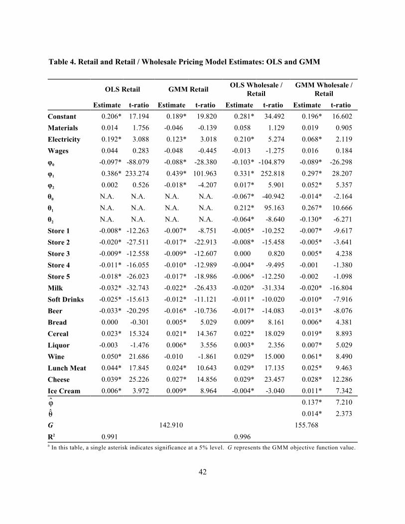
between retailers and manufacturers is critical. Table 4 presents estimates of the shelf-space

pricing model. In order to highlight the importance of including both the retail and wholesale

margin, we present the results from a restricted model in which wholesalers are assumed to be

perfectly competitive (ie., zero margin) and one in which both retailers and wholesalers may earn

non-zero margins. In each case, we present OLS estimates, which are not corrected for

endogeneity, and GMM estimates, which are.

First, note in the retail-margin model that the fitted value of ö suggests a significant

departure from Bertrand-Nash pricing downstream. Because it is less than 1.0, this finding

suggests that retailers price closer to the competitive level than Nash. While deviations below

28

1.0 can be due to either non-linear pricing (Villas-Boas and Zhao, 2005) or omitted competition

from other retailers (Chintagunta, 2002), we account for both of those factors here. Therefore,

we conclude that retailers have an inherent incentive to price more competitively than would

otherwise be the case. By allowing the extent of deviation to depend upon pricing and

assortment strategies, we can provide a better explanation as to the nature of this incentive.

Based on the estimates in table 4, the downstream margin appears to be positively correlated with

prices, which makes intuitive sense. By including retail prices in the margin expression, the

estimated effect of increasing variety must be interpreted as a partial effect with retail prices held

constant. All else equal, therefore, retail margins are negatively related to the number of SKUs,

so wholesale prices must rise with variety. Retailers may be willing to take lower margins if

offering more products tends to build volume at the expense of rival stores, so manufacturers are

willing to pay higher prices for access to their shelves. This conclusion, however, again ignores

vertical relationships with manufacturers.

In the retail - wholesale margin model, we see that this effect is reversed. In other words,

when the possibility of a positive wholesale margin is accounted for, greater variety is associated

with higher retail margins, but lower wholesale, or manufacturer margins. This finding is

consistent with the hypothesis described above. Namely, retailers understand that their

downstream pricing power rises in the number of SKUs they stock. Therefore, as retail surplus

rises in either a higher willingness to pay from the marginal retail customer, or a greater number

of inframarginal customers, manufacturers compete more intensely for a share of the retail

profits. This competition causes retailers to force wholesale prices lower (thus raising retail

margins), and accept correspondingly lower prices for their shelf space. Although wholesale

29

prices are lower, the positive feedback effect that characterizes all two-sided markets arises

through retailers’ reducing the price of access in order to attract more manufacturers and, hence,

raise their own margins by further increasing the number of products on the shelf.

As a corollary to these results, our finding suggests that the demand for shelf-space from

manufacturers is in some sense more important to retailer’s pricing decisions than is consumers’

demand for variety. In other words, retailers would rather subsidize manufacturer’s access to

distribution in order to build pricing power than reduce retail prices in order to build the size of

the network. This is opposite to Kaiser and Wright (2006) who find that magazine publishers

have an incentive to subsidize subscribers in order to increase demand for the medium, and

charge advertisers higher prices to offset the lost subscriber revenue. With retail margins rising in

the depth of assortment, our findings suggest that the supermarkets in our data would rather make

money from the buy rather than on the sell, perhaps explaining the rise of retailers such as Target

and Wal-Mart that do not accept slotting fees and rather set low retail prices in order to maximize

customer traffic.

Another way of thinking of this result is in terms of how expanding the size of the

network influences the pricing power of retailers and manufacturers. By offering a wider

selection of products, retailers have greater pricing power over the downstream market because

consumers’ willingness to pay rises in variety. Manufacturers, however, have less market power

over retailers because by increasing the number of products on their shelves, retailers are

essentially allowing for more competition for shelf space. More competition means lower

margins and less surplus available to pay for shelf-space access.

30

[table 4 in here]

Simulating the Impact of Network Size

In equilibrium, the price of shelf space is equal to the total margin. The impact of expanding the

number of products offered on shelf prices, therefore, depends on the net effect on both retail and

2 2manufacturer margins. Although the relative size of the ö and è parameters is clear from table

4, we demonstrate the net effect more formally, and on a per-store basis through numerical

simulation. Based on the hypothesis tests conducted in the previous section, we expect that

increasing the number of products on offer in a typical category will have the effect of decreasing

wholesale margins and increasing retail margins. How the net effect influences shelf-space

prices, which must equal the total margin in equilibrium, remains an empirical question. From

the results reported in table 5, shelf prices fall in the number of products uniformly across our

sample. In equilibrium, therefore, retail managers induce manufacturers to increase the supply of

new products by reducing shelf prices, which increases consumer demand, raises retail margins

and provides further incentive for retailers to attract new manufacturers. Two-sided retail

demand, while fundamentally different from that witnessed in either technology or media

markets, is nonetheless a significant driver of retail strategy.

[table 5 in here]

Conclusions

31

As intermediaries between manufacturers and consumers, retailers must manage a two-sided

demand for their services. Consumers demand the products retailers stock on their shelves, while

manufacturers demand shelf space for distribution purposes. In this study, we present a

theoretical model of indirect network effects in supermarket retailing and estimate how these

effects impact pricing and assortment strategy among a small set of competing retailers.

We estimate a hybrid CES / nested logit model of store choice using two-years of weekly

scanner data from the top 6 supermarkets in Visalia, California. The econometric model captures

consumers’ preference for variety, as well as potential network effects due to changes in

assortment depth, defined as the number of SKUs stocked per category per week. The CES /

nested logit model is defined at the “shopping basket” level, meaning that we include data from

the top 10 categories in each store to measure store choice probabilities. Using parameters

estimated from the CES / nested logit model, we estimate a second-stage model of supermarket

pricing and assortment behavior in which we allow for non-linear pricing contracts between

retailers and manufacturers and Nash behavior among retailers. With this non-linear pricing

model, we are able to identify prices for store shelves, which are commonly unobserved in

studies of retail pricing and vertical contracting.

Our results show that consumers exhibit a strong preference for variety, or assortment

depth. Because of their preference for variety, and the fact that consumers single-home in a

multi-platform retail environment, retailers have an incentive to reduce shelf prices to

manufacturers in order to increase the number of products on their shelves. Manufacturers, in

turn, are willing to accept lower upstream margins as assortment depth rises, in order to compete

for a share of the higher retail margins that result. This finding has a number of implications for

32

retail strategy, and explains many of the recent trends observed in the supermarkets industry.

Namely, charging excessive slotting fees is not the best way to exploit the two-sided demand

faced by all retailers. Rather than subsidize consumers in order to make money from suppliers,

as is the case in the yellow pages and magazine industries, retailers should do the opposite in

order to build retail margins on the items they sell. Among the different platforms currently

operating in the supermarket industry, traditional supermarkets generally follow a yellow-pages

type of model, while successful and emerging platforms such as Super Target and Wal-Mart

follow the strategy suggested by our research.

33

References

Anderson, S. P. and de Palma, A. 1992. “Multiproduct Firms: A Nested Logit Approach.”Journal of Industrial Economics 40: 261-275.

Armstrong, M. 2006. “Competition in Two-Sided Markets.” RAND Journal of Economics 37:668-681.

Basu, A., T. Mazumdar, and S. P. Raj. 2003. “Indirect Network Externality Effects on ProductAttributes.” Marketing Science 22: 209-221.

Berry, S. 1994. “Estimating Discrete-Choice Models of Product Differentiation.” Rand Journalof Economics 25: 242-262.

Berry, S., J. Levinsohn, and A. Pakes. 1995. “Automobile Prices in Market Equilibrium.”Econometrica 63: 841-890.

Berto Villas-Boas, S. 2007. “Vertical Relationships Between Manufacturers and Retailers:Inference with Limited Data.” Review of Economic Studies 74: 625-652.

Bonnet, C., P. Dubois and M. Simioni. 2006. “Two Part Tariffs versus Linear Pricing BetweenManufacturers and Retailers: Empirical Tests on Differentiated Products Markets.” workingpaper, University of Toulouse, Toulouse, France.

Caillaud, B. and B. Jullien. 2003. “Chicken and Egg: Competition Among IntermediationService Providers.” RAND Journal of Economics 34: 309-328.

Cardell, N. S. 1997. “Variance Components Structures for the Extreme Value and LogisticDistributions.” Econometric Theory 13: 185-213.

Chintagunta, P. K. 2002. "Investigating Category Pricing Behavior at a Retail Chain." Journal ofMarketing Research 39: 141-154.

Church, J. and N. Gandal. 1992. “Network Effects, Software Provision, and Standardization.”Journal of Industrial Economics 40: 85-103.

Cotterill, R. 1986. “Market Power in the Retail Food Industry: Evidence from Vermont.” Reviewof Economics and Statistics 68: 379-386.

Dixit, A. K. and J. E. Stiglitz. 1977. “Monopolistic Competition and Optimum ProductDiversity.” American Economic Review 67: 297-308.

34

Doganoglu, T., and J. Wright. 2006. “Multihoming and Compatibility.” International Journal ofIndustrial Organization 24: 45-67.

Draganska, M. and D. Jain. 2005. “Product-Line Length as a Competitive Tool.” Journal ofEconomics and Management Strategy 14: 1-28.

Draganska, M. and D. Klapper. 2007. “Retail Environment and Manufacturer CompetitiveIntensity.” Journal of Retailing 83: 183-198.

Farrell, J. and G. Saloner. 1992. “Converters, Compatibility and the Control of Interfaces.”Journal of Industrial Economics 40: 9-35.

Gandal, N. 1994. “Hedonic Price Indexes for Spreadsheets and an Empirical Test of NetworkExternalities.” RAND Journal of Economics 25: 161-170.

Gandal, N., M. Kende, and R. Rob. 2000. “The Dynamics of Technological Adoption inHardware / Software Systems: The Case of Compact Disk Players.” RAND Journal of Economics31: 43-62.

Hamilton, S. 2003. “Slotting Allowances as a Facilitating Practice by Food Processors inWholesale Grocery Markets: Profitability and Welfare Effects.” American Journal ofAgricultural Economics 85: 797-813.

Hamilton, S. and T. J. Richards. 2007. “Product Differentiation, Store Differentiation, and theBreadth of Retail Product Assortments.” Working paper, Department of Economics, OrfaleaCollege of Business, California Polytechnic State University.

Kaiser, U. and J. Wright. 2006. “Price Structure in Two-Sided Markets: Evidence from theMagazine Industry.” International Journal of Industrial Organization 24: 1-28.

Katz, M. L. and C. Shapiro. 1985. “Network Externalities, Competition and Compatibility.”American Economic Review 75: 424-440.

Manchanda, P., A. Ansari and S. Gupta. 1999. “The ‘Shopping Basket:’ A Model forMulticategory Purchase Incidence Decisions.” Marketing Science 18: 95-114.

Martinez, S. 2007. “The U.S. Food Marketing System: Recent Developments, 1997 - 2006.”ERR-42. Economic Research Service, USDA. Washington, D.C.

Nair, H., P. Chintagunta, and J.-P. Dube. 2004. “Empirical Analysis of Indirect Network Effectsin the Market for Personal Digital Assistants.” Quantitative Marketing and Economics 2: 23-58.

Peng, S. K. and T. Tabuchi. 2007. “Spatial Competition in Variety and Number of Stores.”

35

Journal of Economics and Management Strategy 16: 227-253.

Richards, T. J. and S. Hamilton. 2006. “Rivalry in Price and Variety Among SupermarketRetailers.” American Journal of Agricultural Economics 88: 710-726.

Rochet, J. -C. and J. Tirole. 2002. “Cooperation among Competitors: Some Economics ofPayment Card Associations.” RAND Journal of Economics 33: 549-570.

Rochet, J. -C. and J. Tirole. 2003. “Platform Competition in Two-Sided Markets.” Journal of theEuropean Economic Association 1: 990-1029.

Rysman, M. 2004. “Competition Between Networks: A Study of the Market for Yellow Pages.”Review of Economic Studies 71: 483-512.

Slade, M. E. 1995. “Product Rivalry with Multiple Strategic Weapons: An Analysis of Price andAdvertising Competition.” Journal of Economics and Management Strategy 4: 445-476.

Smith, H. 2004. “Supermarket Choice and Supermarket Competition in Market Equilibrium.”Review of Economic Studies 71: 235-263.

Villas-Boas, J. M. and Y. Zhao. 2005. “Retailer, Manufacturers and Individual Consumers:Modeling the Supply Side in the Ketchup Marketplace.” Journal of Marketing Research 42: 83-95.

36

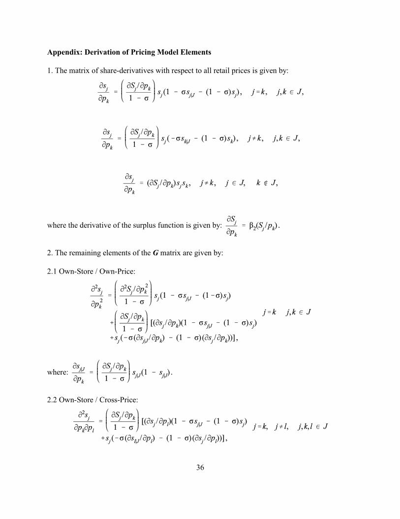
Appendix: Derivation of Pricing Model Elements

1. The matrix of share-derivatives with respect to all retail prices is given by:

where the derivative of the surplus function is given by:

2. The remaining elements of the G matrix are given by:

2.1 Own-Store / Own-Price:

where:

2.2 Own-Store / Cross-Price:

37

where:

2.3 Cross-Price / Second Derivative:

2.4 Cross-Price / Cross-Price:

Table 1a. Summary of Visalia Retail Data by StoreUnits Mean Std. Dev. Minimum Maximum Obs.

Price $ 0.186 0.177 0.017 1.149 1122

No. SKUs / Category Count 139.407 63.679 13.513 355.000 1122

Category Share of Market Share 0.006 0.012 0.000 0.077 1122

Store 1 Category Share of Store Share 0.129 0.050 0.038 0.397 1122

Material Price Index 105.959 71.725 0.106 423.800 1122

Utility Price Index 0.095 0.003 0.090 0.100 1122

Retailing Wage Index 680.342 12.752 653.660 706.850 1122

Price $ 0.138 0.099 0.017 0.523 1122







Price $ 0.196 0.201 0.015 1.027 1122







Price $ 0.187 0.168 0.018 0.798 1122







Price $ 0.185 0.166 0.018 0.984 1122







Price $ 0.197 0.193 0.019 1.034 1122







39

Table 1b. Summary Data for Category Price / Assortment Depth by Store and Category

LowFat

Milk

RegularSoft

DrinksBeer Bread Cereal Liquor Wine

LunchMeat

CheeseIce

CreamOther

Average Product Price ($/oz)

Store 11 0.026 0.059 0.021 0.125 0.226 0.110 0.621 0.333 0.284 0.121 0.116

Store 2 0.024 0.050 0.018 0.119 0.165 0.090 0.289 0.317 0.196 0.169 0.075

Store 3 0.024 0.058 0.021 0.131 0.197 0.082 0.732 0.329 0.309 0.157 0.112

Store 4 0.029 0.062 0.023 0.125 0.223 0.085 0.606 0.336 0.297 0.142 0.125

Store 5 0.029 0.062 0.022 0.124 0.218 0.085 0.596 0.327 0.291 0.155 0.124

Store 6 0.029 0.061 0.023 0.123 0.217 0.088 0.713 0.341 0.285 0.156 0.127

Average Number of SKUs per Category

Store 1 37.93 116.52 158.58 156.08 188.25 167.49 217.30 159.78 159.91 154.68 16.95

Store 2 16.93 67.34 137.43 128.19 177.16 106.89 86.33 111.93 144.82 120.63 15.31

Store 3 30.13 118.42 150.48 130.99 188.76 223.63 220.27 152.12 165.18 102.26 18.06

Store 4 27.00 130.77 158.57 159.61 204.87 219.32 328.89 154.09 181.71 163.31 20.64

Store 5 24.90 141.77 156.78 149.11 189.12 213.61 273.03 147.47 181.90 137.26 19.82

Store 6 26.15 122.43 164.37 140.71 184.09 204.53 265.91 147.54 164.72 131.31 18.42

Simple correlation between average price and number of SKUs = 0.639. 1

40

Table 2. Nested Logit / CES Demand Estimates

OLS Estimates GMM Estimates

Estimate t-ratio Estimate t-ratio

Constanta -2.223* -36.796 -2.555* -28.227

Price -0.237* -19.664 -0.166* -6.051

SKUs 0.312* 25.799 0.064* 5.122

Discount 0.020* 3.215 0.011 1.447

Discount*Price -0.008* -2.996 -0.005 -1.906

ó 0.878* 125.334 0.857* 53.454

Store 1 -0.027* -4.641 -0.033* -4.486

Store 2 0.085* 11.012 0.010 0.555

Store 3 -0.022* -3.721 -0.037* -4.266

Store 4 0.023* 3.704 0.052* 5.202

Store 5 0.018* 2.945 0.030* 4.220

Low Fat Milk -2.689* -128.746 -2.758* -28.354

Regular Soft Drinks -3.959* -146.966 -3.677* -89.973

Beer -3.206* -82.593 -3.033* -28.116

Bread -4.675* -181.385 -4.271* -78.991

Cereal -5.212* -187.525 -4.720* -59.240

Liquor -4.904* -162.301 -4.487* -86.916

Wine -8.122* -173.080 -8.108* -69.970

Lunch Meat -5.702* -228.426 -5.252* -57.929

Cheese -5.774* -218.692 -5.294* -61.424

Ice Cream -8.606* -154.369 -9.301* -160.341

R2 0.997

G 0.472

Hausman ÷2 499.318

In this table, a single asterisk indicates significance at a 5% level. G indicates the GMM objective function value. a

Instruments for the GMM estimator include input prices, input price / category interactions, store, category and

seasonal dummies as well as lagged share values.

41

Table 3. Matrix of Own- and Cross-Price Store Choice Elasticities

Elasticity of Row Store with Respect to Column Store:

Store 1 Store 2 Store 3 Store 4 Store 5 Store 6

Store 1a -3.355 0.552 0.383 0.793 0.753 0.471

Store 2 0.344 -3.024 0.366 0.758 0.720 0.451

Store 3 0.354 0.543 -3.279 0.780 0.741 0.464

Store 4 0.350 0.536 0.372 -2.839 0.731 0.458

Store 5 0.351 0.537 0.373 0.772 -2.885 0.459

Store 6 0.351 0.539 0.374 0.773 0.735 -3.166

The elasticities in this matrix represent averages over all categories for each store. Substitution elasticities fora

individual categories show a similar pattern to the averages shown here.

42

Table 4. Retail and Retail / Wholesale Pricing Model Estimates: OLS and GMM

OLS Retail GMM RetailOLS Wholesale /

RetailGMM Wholesale /

Retail

Estimate t-ratio Estimate t-ratio Estimate t-ratio Estimate t-ratio

Constant 0.206* 17.194 0.189* 19.820 0.281* 34.492 0.196* 16.602

Materials 0.014 1.756 -0.046 -0.139 0.058 1.129 0.019 0.905

Electricity 0.192* 3.088 0.123* 3.018 0.210* 5.274 0.068* 2.119

Wages 0.044 0.283 -0.048 -0.445 -0.013 -1.275 0.016 0.184

0ö -0.097* -88.079 -0.088* -28.380 -0.103* -104.879 -0.089* -26.298

1ö 0.386* 233.274 0.439* 101.963 0.331* 252.818 0.297* 28.207

2ö 0.002 0.526 -0.018* -4.207 0.017* 5.901 0.052* 5.357

0è N.A. N.A. N.A. N.A. -0.067* -40.942 -0.014* -2.164

1è N.A. N.A. N.A. N.A. 0.212* 95.163 0.267* 10.666

2è N.A. N.A. N.A. N.A. -0.064* -8.640 -0.130* -6.271

Store 1 -0.008* -12.263 -0.007* -8.751 -0.005* -10.252 -0.007* -9.617

Store 2 -0.020* -27.511 -0.017* -22.913 -0.008* -15.458 -0.005* -3.641

Store 3 -0.009* -12.558 -0.009* -12.607 0.000 0.820 0.005* 4.238

Store 4 -0.011* -16.055 -0.010* -12.989 -0.004* -9.495 -0.001 -1.380

Store 5 -0.018* -26.023 -0.017* -18.986 -0.006* -12.250 -0.002 -1.098

Milk -0.032* -32.743 -0.022* -26.433 -0.020* -31.334 -0.020* -16.804

Soft Drinks -0.025* -15.613 -0.012* -11.121 -0.011* -10.020 -0.010* -7.916

Beer -0.033* -20.295 -0.016* -10.736 -0.017* -14.083 -0.013* -8.076

Bread 0.000 -0.301 0.005* 5.029 0.009* 8.161 0.006* 4.381

Cereal 0.023* 15.324 0.021* 14.367 0.022* 18.029 0.019* 8.893

Liquor -0.003 -1.476 0.006* 3.556 0.003* 2.356 0.007* 5.029

Wine 0.050* 21.686 -0.010 -1.861 0.029* 15.000 0.061* 8.490

Lunch Meat 0.044* 17.845 0.024* 10.643 0.029* 17.135 0.025* 9.463

Cheese 0.039* 25.226 0.027* 14.856 0.029* 23.457 0.028* 12.286

Ice Cream 0.006* 3.972 0.009* 8.964 -0.004* -3.040 0.011* 7.342

0.137* 7.210

0.014* 2.373

G 142.910 155.768

R2 0.991 0.996

In this table, a single asterisk indicates significance at a 5% level. G represents the GMM objective function value. a

43

Table 5. Impact of Changing Assortment Depth on Equilibrium Prices for Shelf-Space

Store 1 Store 2 Store 3 Store 4 Store 5 Store 6

Price $0.279 $0.206 $0.293 $0.280 $0.277 $0.295

Marginal Cost $0.115 $0.111 $0.115 $0.114 $0.113 $0.115

Shelf-Space Price (N - 50%) $0.159 $0.090 $0.172 $0.162 $0.159 $0.175

Shelf-Space Price (N - 25%) $0.158 $0.090 $0.171 $0.161 $0.159 $0.174

Shelf-Space Price (Base Case) $0.157 $0.089 $0.170 $0.160 $0.158 $0.173

Shelf-Space Price (N + 25%) $0.156 $0.088 $0.170 $0.159 $0.157 $0.172

Shelf-Space Price (N + 50%) $0.155 $0.087 $0.169 $0.158 $0.156 $0.171

network externalities in supermarket retailingshamilto/papers/network_ext_paper_4_08.pdfrecognizing...

Documents