New evidence of a tropical mean 1K stratospheric bias in radiosonde

temperatures in the 1980s from an intercomparison of (un)adjusted

radiosonde data, ERA-40 reanalyses and MSU retrievals

LEOPOLD HAIMBERGER and CHRISTINA TAVOLATO1

submitted to J. Climate, 2 March 2007

1Department of Meteorology and Geophysics, University of Vienna, Althanstrasse 14,

A-1090 Vienna, Austria

Email address: leopold.haimberger@univie.ac.at

2

Abstract

The discrepancy between global mean temperature series from homogenized radiosondes

and temperature series derived from Microwave Sounding Unit (MSU) radiances is a long

standing problem in upper air climatology.

This paper provides new evidence that the gradual cooling of tropical and global mean

lower stratospheric radiosonde temperatures compared to satellite data since the early 1980s

is the composite effect of shifts with size larger than 0.5 K in individual radiosonde time

series. The breaks have been detected with an automatic method (RAdiosonde OBservation

COrrection using REanalyses - RAOBCORE). The differences between satellite products

and time series of ERA-40+ECMWF background forecasts (BG) are much smaller, on the

order 0.2 K, even on regional (10◦ × 10◦) scales. The warm bias of radiosondes in the 1980s

is estimated 0.6±0.2 K in the global mean, and 1.0±0.3 K in the tropical (20◦S-20◦N) mean

for the MSU lower stratosphere (LS) equivalent layer. A similar comparison for MSU-3

(upper tropospheric) layer mean temperatures yielded radiosonde temperature biases of

0.35± 0.1 K in the global mean and 0.5± 0.2 K in the tropical mean in the late 1980s

RAOBCORE uses the BG data as reference for homogenization. The consistency of

the BG with MSU satellite products from 1987 onwards is quite high although it has been

created with substantially different algorithms for assimilating the radiances. Only before

1987 some shifts in the global mean have been detected that must be removed before

using the BG as reference for homogenization. Due to the better understanding of the

background behaviour, the uncertainty estimates for the homogenized radiosonde dataset

could be reduced compared to a recent paper on RAOBCORE. The resulting adjusted

radiosonde time series are in much better agreement with satellite data than was the case

in recent satellite-radiosonde intercomparisons.

At high latitudes sizeable seasonally varying differences between individual radiosondes

and satellite data remain after homogenization. These are partly related to seasonal varia-

tions of the daytime radiation error, which are not adjusted by RAOBCORE. Still existing

3

difficulties in capturing during wintertime sudden stratospheric warming (SSW) events in

the satellite data, and representation errors (radiosonde point measurement vs. 2.5 degree

average) also contribute to the differences.

4

1. Introduction

Despite much research in upper air observations there is still sizeable discrepancy be-

tween layer mean atmospheric temperatures derived from radiances of the Microwave Sound-

ing Unit (MSU) and MSU-equivalent temperatures calculated from radiosonde data (see

e.g. Santer et al. 2005; Karl et al. 2006). Mears et al. (2006) suspect that especially the

lower stratospheric time series from radiosondes are biased and Sherwood et al. (2005) and

Randel and Wu (2006) have described pervasive daytime biases in the tropics. However

this evidence has been fragmentary so far and the biases have not been quantified for global

or latitudinal belt means.

With the advent of the Integrated Global Radiosonde Archive (IGRA, Durre et al. 2006)

and of the so-called ERA-40 analysis feedback dataset (Uppala et al. 2005), amended

with the operational European Centre for Medium-Range Weather Forecasts (ECMWF)

analysis feedback from 2001 onwards, the density of radiosonde datasets has recently been

improved. Both datasets reach back to at least 1958 and are input of the RAOBCORE

(RAdiosonde OBservation COrrection using REanalyses) dataset (Haimberger 2007), which

contains more than 1000 adjusted radiosonde temperature time series.

The only homogenized radiosonde dataset with comparable station number is the Hadley

Centre upper Atmospheric Temperature (HadAT) dataset (Thorne et al. 2005). It is based

on the Comprehensive Atmospheric Radiosonde DataSet (CARDS, Eskridge et al. 1995)

and is updated with IGRA data (McCarthy et al. 2006). The so-called ”radiosonde at-

mospheric temperature products for assessing climate” (RATPAC, Free and Seidel 2005)

is based on much less (ca. 80) radiosonde stations. A crude intercomparison of these three

datasets in terms of global and tropical belt means can be found in Christy and Coauthors

(2007), where they appear quite consistent, except in the lower stratosphere in the satellite

era, where RATPAC and HadAT dataset show stronger cooling. A more detailed intercom-

parison is left for the future. Here we focus on the comparison of RAOBCORE-adjusted

radiosonde data with MSU and ERA-40 data.

5

From 1979 onwards the radiosonde data can be compared with MSU brightness tem-

peratures representative for thick vertical layers. We used Remote Sensing Systems (RSS)

3.0 (Mears et al. 2003; Mears and Wentz 2007) and University of Alabama at Huntsville

(UAH) v5.1 (v5.2 for LT) (Christy et al. 2003) brightness temperatures representative for

the lower stratosphere (LS), mid-troposphere (MT) and lower troposphere (LT). Data from

Vinnikov et al. (2006) have not yet been analysed. They show stronger warming trends

than any other MT equivalent dataset.

Much less attention has been paid to the MSU3 channel in recent years, because it

samples a very thick layer (peak sensitivity at ca. 250 hPa) in the upper troposphere and

lower stratosphere. It is referred to as TS layer. Due to the unusual behaviour of the MSU3-

radiances on NOAA-9 and due to a data gap in 1986, which is very difficult to handle (Mears

et al. 2006; Uppala et al. 2005), TS products are available only from RSS and only from

1987 onwards. However, radiances from this channel are routinely assimilated in climate

data assimilation systems such as ERA-40 and have substantial influence on the analysed

upper tropospheric temperatures.

Previous studies performed radiosonde data vs. MSU data comparisons only for rather

large latitudinal belts (e.g. Lanzante et al. 2003; Seidel et al. 2004; Free and Seidel

2005; Santer et al. 2005) or for relatively small subsets of the available radiosonde dataset

(Christy and Norris 2006; Christy and Coauthors 2007; Randel and Wu 2006). This paper

presents selected results from a more comprehensive and regionally detailed comparison

between MSU and radiosonde datasets.

The radiosonde data basis for this comparison is the RAOBCORE dataset (Haimberger

2007). It contains both the raw radiosonde data as well as the time series homogenized

with an automatic algorithm that uses the ERA-40 and ECMWF operational background

forecast time series (hereafter referred to as BG) as reference. Haimberger (2007) has shown

that the RAOBCORE adjustments make the radiosonde data spatially more consistent and

remove most of the artificial trends in the diurnal temperature cycle. The reader is reminded

6

that the background forecasts are used as reference, not the analyses, since they are better

suited for observation bias estimation (Dee 2005).

Despite these merits there has still been relatively large uncertainty in the global mean

trends from this dataset on the order of 0.3 K/decade for the LS layer, mainly because for

some time periods the BG has been found questionable (Haimberger 2007; Uppala et al.

2005; Trenberth and Smith 2006; Karl et al. 2006). In order to better assess the quality

of the BG time series used as reference and thus to better constrain the uncertainties

involved in the radiosonde adjustments, a detailed intercomparison between satellite data,

radiosonde data and the ERA-40 background has been undertaken.

In the next two sections, the input data and the comparison method are described in

some detail. In section 4 some intercomparisons for the MSU LS and TS equivalent layer for

individual radiosonde time series are presented. In section 5 global belt mean comparisons

are discussed and it is shown how the discrepancy between unadjusted radiosondes and

satellite data can be traced back to large breaks detected in the radiosonde time series.

Also the effect of some difficulties of the BG dataset in the early 1980s could be quantified.

Implications of these results are discussed in section 6.

2. Input data

The following input data have been used for this intercomparison:

• RSS MSU v3.0 data (Mears and Wentz 2007) on the standard 2.5×2.5◦ lat/lon grid

at all available layers (LS, TS, MT, LT).

• UAH MSU v5.1 data (5.2 for LT) (Christy et al. 2003) on the standard 2.5×2.5◦

lat/lon grid at all available layers (LS,MT, LT). The RSS and UAH temperature

datasets have been calculated from the same raw radiance datasets, though with

quite different analysis methods. The main uncertainties arise from the connection

of data from different satellite platforms which often have rather short overlap time

and from the correction of drift effects.

7

• Homogenized 2m temperatures from HADCRUTv3.0 (Brohan et al. 2006) on a

5 × 5◦ lat/lon grid. These are needed for calculating MSU MT and LT equivalent

layer mean temperatures from BG and radiosonde observations.

• ERA-40/ECMWF background forecasts (BG) and analyses on a 1.25×1.25◦ lat/lon

grid and interpolated to radiosonde stations. The BG used for the period 1979-

2000 is the product of a comprehensive data assimilation procedure that uses most

available observations, including radiosondes, surface temperatures and satellite ra-

diances. The data for ERA-40 have been assimilated with a 3D-VAR (First Guess

at Appropriate Time - FGAT, Uppala et al. 2005) system which is beneficial for

assimilation of satellite radiances, especially if there are orbital drifts. The BG

temperatures are used at 00GMT and 12GMT, which implies that the background

forecasts are started with analyses at 06GMT and 18GMT, when very little ra-

diosonde information is available. Due to the large differences in the assimilation

system compared to UAH and RSS it is by no means clear that the resulting tem-

perature time series are consistent with the RSS and UAH satellite retrievals.

From 2001 onwards operational ECMWF background forecasts have been used.

These are 12h forecasts gained with a 12h 4D-VAR system. There is still large

influence of the satellite observing system.

The fraction of information content coming from radiosondes is relatively small

especially in the recent ECMWF-analyses (Cardinali et al. 2004). However, the

influence of radiosondes on biases may be larger since the bias correction procedure

applied in ERA-40 and in ECMWF operations until early 2006 (Harris and Kelly

2001) heavily relies on comparison with a subset of high quality radiosondes.

• The RAOBCORE dataset (http://www.univie.ac.at/theoret-met/research/raobcore/;

Haimberger 2007). The source for RAOBCORE are the IGRA and the ERA-

40/ECMWF radiosonde archives. Metadata information could be extracted from

8

Gaffen (1996) and from the ERA-40 feedback records (Haimberger 2007) which often

include the radiosonde type routinely transmitted by many stations.

The homogenized radiosonde data used in this paper (version 1.4) have been

generated as described in Haimberger (2007), with the exception that an ERA-40

background correction as described in this paper has been applied only prior to

1987. As will be shown below, the unadjusted BG is quite consistent with satellite

estimates after 1987. Only before 1987 some unphysical signals are evident in the

BG which need adjustment.

In the RAOBCORE-dataset documented in Haimberger (2007) (version 1.2) the

global mean background has been adjusted also after 1987 towards the unadjusted

radiosonde dataset. Haimberger (2006) has shown that this adjustment reduces

the good consistency of the global and tropical mean BG with the UAH and RSS

satellite products after 1987, which is of course undesirable.

3. Comparison method

3.1. Construction of the MSU equivalents.

The radiosonde data as well as the ERA-40/ECMWF operational products are available

on standard pressure levels (10, 20, 30, 50, 70, 100, 150, 200, 250, 300, 400, 500, 700, 850

hPa) and are valid for the station location. From these MSU equivalent layer means can be

calculated. The necessary weighting functions for the LS, MT and LT layers are the same

as used by Thorne et al. (2005). For the TS layer, weighting functions have been provided

by C. Mears (pers. comm.).

While the LS and TS layers are insensitive to the Earth’s surface properties (except

possibly the TS layer over elevated terrain), the MT and LT equivalent temperatures need

surface temperature information for their calculation. HadCRUT3 temperature data have

been used for this purpose.

3.2. Construction of anomalies.

9

MSU equivalent time series have been calculated from radiosonde data and BG data

separately for 00GMT and 12 GMT. At least 10 values per month have been necessary to

yield a monthly mean value. The RSS and UAH data have been taken as available and can

be interpreted as monthly daily means.

The satellite products are available as anomalies with respect to the 1979-1998 clima-

tology and the BG and radiosonde data have been divided into climatologies and anomalies

as well. Much care is needed for this task, especially if the time series contain large and

highly transient climatological signals such as SSWs and if values are missing. The large

amplitude of these warmings (up to 15 K in the anomalies of LS MSU equivalents, Limpa-

suvan et al. 2004; Charlton and Polvani 2007; Charlton et al. 2007) have the potential

to substantially influence the climatologies. Consequently, the climatology of a station at

high latitudes with a few January values missing may be quite different from a station with

these values, if SSWs occured in these months. Therefore climatologies and anomalies have

been calculated only if at least 15 out of 20 years have been available, and only for those

months that have been available in all (MSU, BG and radiosonde) datasets noted above.

This procedure guarantees that differences between datasets at individual stations cannot

be related to missing monthly data.

3.3. Horizontal interpolation and sampling.

This paper reports about individual station intercomparisons as well as about global

scale intercomparisons on a monthly time scale. The radiosonde data and the BG data

are valid at the observation locations. The nearest gridpoint with MSU data, which are

available on a 2.5◦×2.5◦ grid, has been used for station by station intercomparisons. The

HadCRUTv3.0 data are available only at 5◦×5◦ resolution. Points on a 2.5◦×2.5◦ grid

have been calculated using bilinear interpolation. This should be accurate enough for the

large-scale features considered.

Only radiosonde time series with less than 25 months of missing data in the 27 year

period considered have been included in the global and tropical belt mean intercomparisons.

10

The 24 month threshold is necessary for a stable trend calculation. Fig. 1 shows LS-

equivalent trends of all the radiosonde stations that fulfil this criterion.

One problem in comparing radiosonde and MSU data is the uneven distribution of

radiosonde data (Free and Seidel 2005). For zonal and global means, we used the following

sampling strategy:

• For each 10◦×10◦ gridbox, a gridbox mean temperature has been calculated from

the continuous radiosonde time series at 00GMT and 12GMT. For some gridboxes

over Europe and China, this is an average over 20 radiosonde time series, for others,

it is only one radiosonde time series. No Indian stations have been used.

• For each 10◦×10◦ gridbox, an average MSU brightness temperature has been cal-

culated from those gridpoints that have been nearest neighbour to a radiosonde

station.

• Each 10◦ latitudinal belt has 36 such gridboxes with values at 00GMT and 12GMT.

These values have been averaged to yield a daily mean zonal belt mean, if at least

2 boxes out of 36 were available. The zonal belt means have been averaged (area-

weighted) to yield global means.

4. Station intercomparisons - two examples

The noise level of difference time series from MSU-equivalent radiosonde temperatures

and MSU satellite retrievals is small enough to allow sensible comparisons for individual

stations. To illustrate the value of such an intercomparison, two representative examples

have been chosen.

Station Bethel (70219, Alaska) has been studied in some detail already by Haimberger

(2007). The comparison of MSU equivalent anomaly time series at this station in Fig. 2

complements the description, at least for the satellite period.

11

Fig. 2 shows differences RSS-RAOBCORE, UAH-RAOBCORE, BG-RAOBCORE and

Unadjusted RS-RAOBCORE of the LS- and TS- equivalent layer mean temperature anom-

aly time series. The time series shown are not time filtered, i.e. unsmoothed monthly mean

curves.

It has been decided to plot differences of anomalies and not anomalies themselves since

the anomalies at high latitudes are very large (15K) during SSWs. The much smaller

differences between the datasets would be hard to spot in a normal anomaly plot.

The fact that the time series in Fig. 2 show differences with respect to RAOBCORE

adjusted radiosonde data does by no means imply that this dataset is the most accurate one.

This type of plot does, however, (i) stress the difference between datasets that may serve as a

reference for radiosonde temperature homogenization (RSS, UAH and BG) and the adjusted

radiosonde data. It (ii) clearly depicts the adjustments subtracted by RAOBCORE, which

are the differences between unadjusted and adjusted radiosonde time series. One should

note that the dark blue curve shows adjustment anomalies. In the most recent part of

the time series, the absolute adjustment is zero at Bethel. Therefore one has to shift the

dark blue curve upward so that it is zero in 2006 in Fig. 2 in order to see the absolute

adjustment.

One can see that the BG data, UAH data and RSS data are in good agreement, compared

to the large differences between unadjusted and adjusted radiosonde datasets. A strong

annual variation of these three anomalies is evident compared to the adjusted radiosonde

anomalies, however. It may have the following reasons:

• Since anomalies are compared, which have been carefully calculated from exactly the

same months for all datasets, the variation cannot come from different calculation

of climatologies.

• Since a constant annual cycle is filtered by using anomalies, the annual cycle visible

in the differences must come from a time-varying annual cycle. One reason for such

a behaviour are the strongly varying radiation errors of the radiosondes used at

12

Bethel (VIZ before 1989, Space Data radiosondes between 1989 and 1995, Vaisala

RS80 from 1995 onwards). This problem has been stressed already in Fig. 10

of Haimberger (2007). Inhomogeneities in the annual cycle are not removed by

RAOBCORE since only constant adjustments with no annual variation are applied.

The similar annual cycles of the RSS-RAOBCORE, UAH-RAOBCORE and BG-

RAOBCORE anomaly differences in Fig. 2 indicate that the problem comes from

the radiosonde measurements. This is further corroborated by the weaker anomaly

differences at 12GMT (nighttime, see panels c) and d) of Fig. 2).

• Representation of SSWs in satellite data may also be a reason. The differences in

annual cycles between UAH and RSS products are largest during the winter months,

when the SSWs occur. The RSS data show slightly better consistency with BG and

radiosondes.

• Representation errors may also contribute to the annual cycle. Whereas the nearest

UAH and RSS gridpoint values are used for radiosonde station comparison, the

BG values are bilinearly interpolated values from the nearest BG gridpoints. This

interpolation is more accurate and is the main reason why the BG comes closest

to the adjusted radiosonde time series. In a sensitivity experiment the BG values

have first been interpolated to a 2.5/2.5 grid (as are the satellite data) and then

the nearest gridpoint value has been used. In this case the annual cycle of the BG

minus RAOBCORE differences showed an amplitude very similar to the anomaly

differences of the satellite data.

The right panels of Fig. 2 show the differences in trends 1979-2006, also with respect to

RAOBCORE-adjusted radiosonde data. In the lower stratosphere the RSS time series is

warming at Bethel relative to UAH and BG, which are quite consistent with the adjusted

radiosonde dataset. The error bars indicate the sampling uncertainty, not the structural

uncertainty. Differences between datasets larger than the error bars are caused by residual

biases in at least one of the datasets. The smaller error bars of the BG-RAOBCORE

13

difference shows that the BG is most consistent with the adjusted radiosonde data. No

error bars have been added to the unadjusted radiosonde data since the error is dominated

by the large spurious cooling trend due to the breaks in the time series.

Fig. 2-b) and d) show a detailed intercomparison of MSU3 (TS) equivalent time series.

This channel has not been used much by climatologists yet because it is affected most

seriously by the NOAA-9 problem in 1986 and because it mixes upper tropospheric and

lower stratospheric temperature signals. However, this channel has large influence in climate

data assimilation systems such as ERA-40. Further it is useful for investigating the strong

warming signal in the tropical upper troposphere predicted by most climate models.

The TS product is not available from UAH and is provided by RSS only from 1987

onwards because of the NOAA-9 problem. Again there is a significant annual variation in

the anomaly differences due to the changing annual cycle of radiosonde radiation errors at

Bethel. Please note that the temperature scale is different in this plot.

The anomaly differences of station Yap (91413, see Fig. 3) in the tropical west Pacific

are an example the large temperature biases at several radiosonde stations in the tropics.

It has several large breaks during the satellite era in the LS layer. The consistency between

BG and RSS/UAH data is again clearly better than the consistency between unadjusted

radiosondes and satellite data. The breaks are so large that they can safely be attributed

to the radiosonde time series. The treatment of MSU radiances in RSS, UAH and ERA-40

is sufficiently different and the uncertainty sufficiently small to exclude the possibility that

these three datasets are affected by a jump in MSU radiances. The adjusted radiosonde

time series shows quite reasonable agreement with the satellite and ERA-40 bg datasets.

Similar large breaks can be found at other tropical stations, e.g. 91348, 91592, 91958.

Below it is shown that the combined effect of these large breaks explains the much stronger

cooling trend in tropical mean temperatures derived from radiosondes. In the TS layer, the

picture is similar, although not quite as clear.

14

Plots as shown in Figs. 2 and 3 are available in the internet (http://www.univie.ac.at/theoret-

met/research/RAOBCORE) for more than 600 radiosonde stations for which climatologies

could be calculated. They allow a systematic station by station evaluation of the discrep-

ancies between the different datasets and are available also for the MT and LT layer.

5. Global scale comparison of layer mean temperatures

In this section the various temperature time series 1979-2006 are compared using global

maps of trends at individual stations and global belt mean time series.

Fig. 1 shows LS equivalent temperature trends 1979-2006 for the unadjusted and ad-

justed radiosondes. One can see the improved spatial trend homogeneity achieved with

RAOBCORE also for daily mean time series. The adjusted trends are spatially not as

homogeneous as the RSS and UAH trends (not shown; maps are available at the UAH,

RSS and RAOBCORE web sites) but the pattern becomes quite similar, with the strongest

cooling in the subtropics and weaker cooling in the tropics.

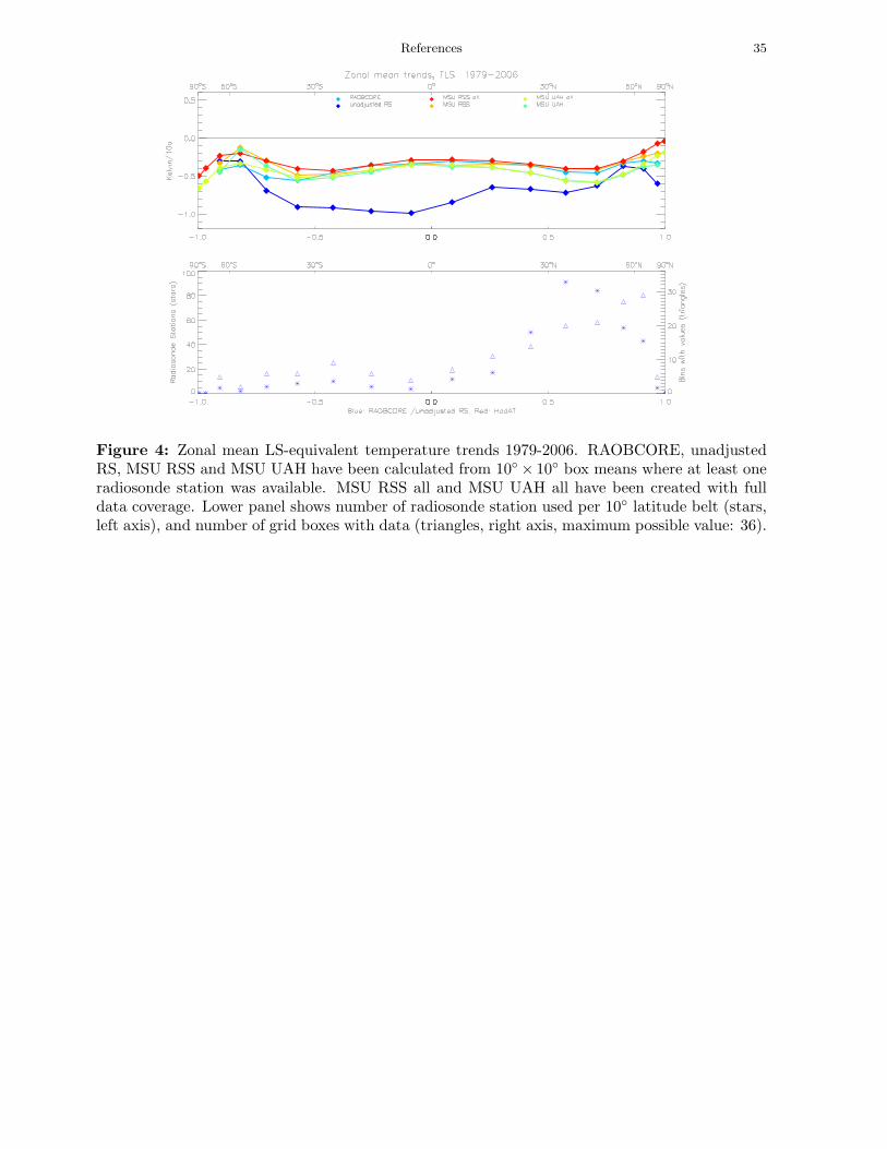
Zonal mean trends 1979-2006 as plotted in Fig. 4 for the LS layer show that the

RAOBCORE adjustments bring the radiosonde trends into good agreement with satellite

and BG data, with the exception of the data-sparse southern extratropics and the very

highest latitudes. The lower panel shows observation coverage i.e. number of stations

per 10◦ latitude belt and the number of 10◦ × 10◦ gridboxes which contain at least one

radiosonde time series that meets the data availability criteria specified above.

While the maps give an impression of the spatial homogeneity of the data, the global

temporal homogeneity is best examined in terms of difference time series of large scale

means. We concentrate on the tropics (20S-20N) and on global means. Fig. 5 shows global

mean anomalies with respect to 1979-1998 for the LS and TS layers. These are well known

in principle but they include the ERA-40 bg and the RAOBCORE-adjusted radiosonde

time series. O

The trends of adjusted radiosonde datasets and satellite data and BG differ by 0.1 K/decade,

whereas the trend difference between unadjusted radiosonde and satellite data is 0.4 K/decade

15

(see table 1 below). The figure contains also time series of the RSS, UAH, BG datasets

and of the ERA-40+ECMWF analysis (AN) with full data coverage (open diamonds). One

sees that ERA-40 background and analyses show very similar trends, with slightly more

negative values for the analyses.

In order to see more detail, the global and tropical mean anomaly difference time series

with respect to the homogenized radiosonde time series are plotted in Figs. 6 and 7 in the

same manner as for the individual stations above. The global anomaly differences in Fig. 6

show the noticeable warming of the RSS MSU and BG data in LS and TS layer compared to

UAH, and adjusted radiosondes. The dark blue line shows the strong adjustment applied by

RAOBCORE in the early 1980s which is gradually reduced as radiosondes have improved.

Note again that these are adjustment anomalies. In 2006 the absolute adjustments are

practically zero.

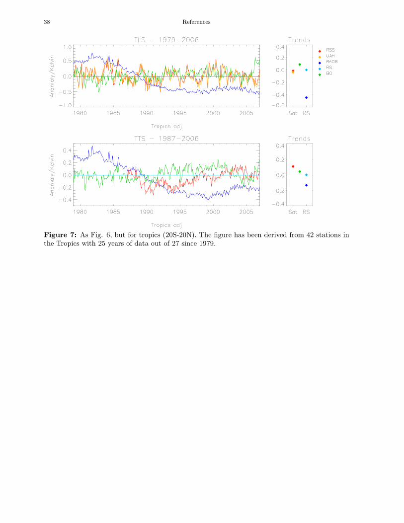
In the following the discussion will focus on the tropics. The temporal consistency of

radiosonde time series, especially at higher altitudes, has been questioned by several authors

(Sherwood et al. 2005; Randel and Wu 2006; Mears et al. 2006) but the results were limited

to a subset of the available data and the attempts to homogenize data were insufficient.

One can see that the differences between adjusted radiosonde data, MSU data and BG

are less than 0.2 K almost everywhere in this unsmoothed monthly time series in Fig. 7.

This consistency is remarkable given the quite different genesis of the plotted data. An

exception are the most recent anomalies in 2006 which are quite different between BG

and the other datasets. The reason is the profound change in the ECMWF operational

assimilation system that has taken place in February 2006 (Untch et al. 2006)

The difference between unadjusted and adjusted radiosonde time series, however, is

large and systematic, for the TS and even more so for the LS layers. The difference curve

summarizes the effect of all adjustments applied by RAOBCORE on the tropical radiosonde

time series, which explains why it is now a relatively smooth curve in contrast to the station

time series. The difference between the dark blue curve in 2006 minus the dark blue curve

16

in the 1980s is the RAOBCORE estimate for the bias of the radiosonde observations in the

1980s. It is 1 K in the tropics and 0.6 K globally in the LS layer. It is 0.5 K in the tropics

and 0.4 K globally in the TS layer.

The differences alone do not imply that the satellite and BG data are right and the

radiosondes are biased. One could still argue that the differences have been generated by

many too liberal homogeneity adjustments that simply draw the radiosonde time series to

the BG time series.

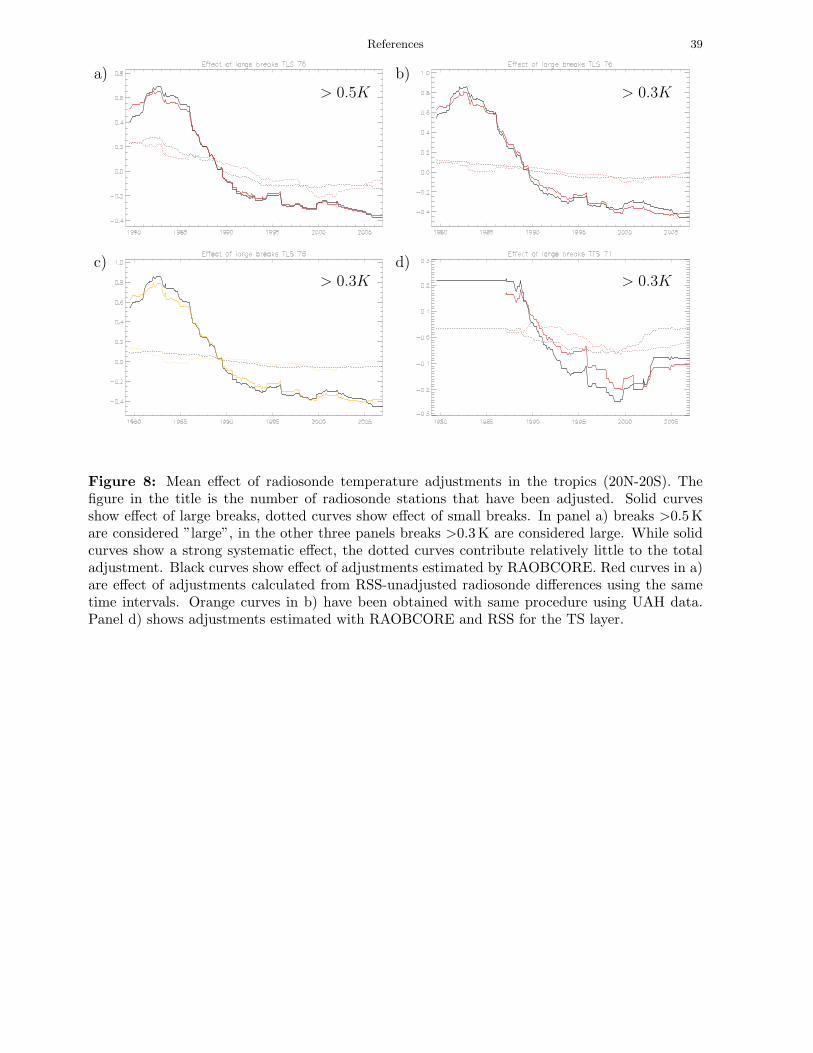
However, Fig. 8 shows that the differences between unadjusted and adjusted radiosonde

temperature anomalies are the composite effect of adjustments of large (>0.3 K) breaks at

individual radiosonde sites. In the LS even the very large (>0.5 K) adjustments explain

most of the effect on trends. Such break sizes are larger than any uncertainty estimate

for the MSU and BG and are also larger than any differences found between these time

series. The break sizes have been estimated by RAOBCORE but also from difference time

series between RSS/UAH MSU data and unadjusted radiosonde data using the same time

intervals for estimating the break sizes as RAOBCORE. The resulting difference show only

a slightly weaker trend, if satellite data are used as reference instead of the BG. There is

little reason to doubt the overall accuracy the temperatures derived from MSU radiances

(despite some difficulties), since they have been assimilated with quite different method and

nevertheless led to similar time series. There is good reason to question the homogeneity

of radiosonde time series, given the large breaks detected in individual station time series,

especially if there are known changes in instrumentation. This is the case for most large

breaks.

We consider this as proof that a large fraction (at least 75%) of the differences between

radiosonde and satellite trends in the LS layer are attributable to problems with radiosondes

in the 1980s. Only in the early 1980s there is a peak in the RAOBCORE adjustments

that is not supported in this magnitude by RSS and UAH. It may be caused by slightly

too cool global mean BG values at this time that have not properly been adjusted before

17

homogenization. The fact that the adjustments in Fig. 8 estimated from the UAH and RSS

data are 0.1-0.2 K weaker in the early 1980s than the RAOBCORE estimates may be an

indication of this problem. On the other hand the trends from the adjusted radiosonde time

series are still more towards cooling than those from satellite time series, which suggests

that the adjustments may be still too weak. Therefore we take the difference of 0.2 K as

measure for the structural uncertainty involved in the adjustment process and thus of the

bias estimates for the early 1980s given above.

The results are qualitatively similar but not as clear for the TS layer (Fig. 7-b and 8-

d). There is only one MSU dataset (RSS) available from 1987 onwards and the differences

between adjusted radiosondes, RSS and BG are larger. Trends from RSS TS data are more

towards warming than the BG and radiosonde data. Shifts between the RSS and the BG

noticeable in 1995 and 2003. Therefore there is currently more uncertainty involved in the

satellite and BG estimates relative to the radiosonde estimates than is the case for the

LS layer. Nevertheless the still large size of the radiosonde adjustments suggest that the

radiosonde temperatures in the TS layer in the early 1980s are at least 0.4 K too warm in

the tropics. It is interesting to note that both satellite data and BG support the composite

mean upward adjustment of tropical mean radiosonde temperatures in the TTS layer in

2002.

RSS does not provide a TS product before 1986 but it is possible to construct a TS

equivalent time series from both radiosondes and ERA-40 background. In order to analyse

the difficulties involved in assimilating MSU3 data in 1986, we have plotted the tropical

temperature anomaly differences gained with two versions of RAOBCORE. In version 1.4

(Fig. 7) that has been used throughout this paper, the global mean background temperature

time series has been adjusted as described in Haimberger (2007) before 1987, as has been

done in all other plots shown in the present paper.

In the second version (v1.3, Fig. 9), no ERA-40 background adjustment has been

applied at all. In this figure one sees a large spurious wiggle in the BG temperature

18

anomaly difference in 1986 and a suspicious cool anomaly of the BG relative to radiosondes

and satellite data between 1980 and 1984. These breaks are likely attributable to problems

in the assimilation of MSU3 and Stratospheric Sounding Unit (SSU) radiances in ERA-40

(Santer et al. 2004; Uppala et al. 2006). Especially the assimilation of the year 1986 has

brought all reanalyses systems to their limits. Little overlap and large gradual changes in

MSU radiances have led to inaccurate bias estimates from static satellite bias correction

schemes (Harris and Kelly 2001) in ERA-40. Results with adaptive bias correction schemes

(Dee 2005; Auligne and McNally 2006) give hope for more accurate bias estimates under

such circumstances.

The wiggle in the uncorrected BG in 1986 can trigger some spurious break detections

in RAOBCORE, if it is not adjusted. This can be seen from dip around 1985/86 in the

unadjusted minus adjusted radiosonde time series (blue curve in Fig. 9) which appears

unrealistic.

Fig. 7 shows that the wiggles in the BG have been efficiently damped in version 1.4. Also

the dark blue composite adjustment time series more realistic, with a monotonic decrease

around 1986. Despite the uncertainty involved in adjusting this wiggle, the large overall

decrease in this difference in the TS layer throughout the 1980s and 1990s can still be

attributed mainly to large (>0.3 K) breaks in the radiosonde time series. This may be seen

also from Fig. 8-d.

6. Trend estimates for zonal belt means

The detailed comparison between satellite data, BG and adjusted radiances has con-

vinced us that the BG time series is quite consistent with satellite products from 1987

onwards in the LS and TS layers and that it should not be adjusted in the global mean

towards unadjusted radiosondes after 1987. An exception is the inhomogeneity in the BG

recently introduced in by a large system upgrade at ECMWF in February 2006, which will

be adjusted using pre-operational test data available from ECMWF.

19

The additional knowledge about the performance of the ERA-40 bg relative to datasets

derived from MSU radiances has resulted in reduced uncertainty estimates for the RAOBCORE-

adjusted radiosonde trends compared to Haimberger (2007). The uncertainties in the global

and tropical mean trends from RAOBCORE adjusted data are likely below 0.1 K/decade

in the MT and LT layers. This value has been found from bootstrapping the global belt

mean time series and from the difference between UAH, RSS, BG and RAOBCORE layer

mean trends. In the TS and LS layers the uncertainty is considered larger, on the order

0.15 K/decade.

Table 1 summarizes trends from LS, TS, MT and LT equivalent layers, where MT

and LT equivalents have been calculated with HadCRUTv3 (Brohan et al. 2006) surface

temperature data.

In general there is very good agreement between RAOBCORE-adjusted data and UAH/RSS

data. In particular in the LS and TS layer it comes closer to these two datasets than any

other homogenized radiosonde dataset (see also Karl et al. 2006; Christy and Coauthors

2007). In the MT layer the RAOBCORE trends are between RSS, BG and UMd (Vinnikov

et al. 2006; not listed) trends and UAH trends. In the LT layer there is good agreement

between all datasets.

The vertical trend profile from RAOBCORE radiosonde time series for the global mean

and the tropical belt mean is shown in Fig. 10. These show a minimum in the RAOBCORE-

adjusted temperature trends in the 500/700 hPa layer and a maximum around 300 hPa. The

maximum in 200-300 hPa in the tropics seems moderate, at least it is only slighly stronger

than the surface or 850 hPa trends. Thus they are broadly consistent with thermodynamic

arguments put forward by Santer et al. (2005); Held and Soden (2006). The minimum in

500-700 hPa, although it occurs also in other radiosonde datasets ((Thorne et al. 2005)),

may not be a robust feature, since it is absent if the trend period is restricted to 1987-2006.

20

Concerning the new TS data included in this intercomparison: They show slight warm-

ing, except in the southern extratropics. The trends are weak in general since they are in-

fluenced by both cooling stratosphere and warming troposphere. The RSS TS v3.0 product

shows more warming than BG and adjusted radiosonde data. The RAOBCORE-adjusted

data show almost neutral trends in the tropics. The necessity of radiosonde temperature

bias adjustment for this layer is also clearly visible from table 1, since the unadjusted global

TS trends are ca. 0.25K/decade cooler than both RSS and BG.

7. Conclusions and Outlook

Haimberger (2007) has introduced the RAOBCORE method and proved its ability to

improve spatial trend consistency and to eliminate spurious changes in the day-night tem-

perature differences but has put little emphasis on the effect on global trends.

This paper has focused on daily mean time series and their trends in the lower strato-

sphere and upper troposphere. It has documented some new evidence of large systematic

tropical mean radiosonde temperature biases in the mid-1980s on the order of 1 K in the LS

equivalent layer. This bias compared to MSU satellite data has been substantially reduced

until the early 1990s with better radiation shielding and better temperature sensors. While

the reduction of the bias appears gradual in the tropical or global mean, it is mainly caused

by large and systematic shifts towards cooler temperatures at individual radiosonde sites,

which often coincide with station metadata events.

The alternative explanation for this change - gradual changes of biases in MSU satellite

data - can be excluded, since these would be visible as gradual changes in satellite minus

radiosonde time series at most stations, which is not the case. In this sense we speak of

evidence although it is not based on agreed transfer standards (Thorne et al. 2005).

Apart from the global belt means, individual station time series at high latitudes have

been studied in some detail to see how sudden stratospheric warmings are represented

in the various datasets. It has been found that the satellite data still have substantial

deviations from the adjusted radiosonde time series, which can be traced back partly to

21

intraseasonal variations of the radiation error, that has not been adjusted by RAOBCORE,

partly to representation errors, and partly to problems in the assimilation of such abrupt

temperature changes by the various assimilation schemes.

While this paper has provided new evidence for the large stratospheric radiosonde tem-

perature bias in the 1980s and the ability of RAOBCORE to adjust this bias, one may

critisize that the adjustment method is neither independent of satellite data nor inde-

pendent of radiosonde data to be adjusted. It would be desirable to adjust the breaks

in radiosonde time series using neighbouring radiosondes only, as done by Thorne et al.

(2005); McCarthy et al. (2006), since then a dataset without reference to MSU data could

be created. The latter have performed several ensemble experiments with an automated

homogenization method based on neighbour intercomparison. Their results indicate that it

is already challenging to remove only half of the biases in a radiosonde network that have

been artificial added to a reference without complete metadata documentation. Sperka

et al. (2007) have developed an adjustment method that uses temporally homogeneous

parts of neighbouring radiosonde time series. The homogeneous parts have been defined as

the time series between breakpoints gained with RAOBCORE. The resulting adjustments

are only slightly weaker than the adjustments presented here. With increasing knowledge

of the breakpoints of radiosonde time series it may be eventually possible to verify the bias

estimates that we have gained here with a pure radiosonde dataset.

During some periods the BG is questionable and Haimberger (2007) developed a method

for adjusting the global mean BG towards the unadjusted radiosondes, but left it open when

it should be applied. Because of the good consistency of the satellite-equivalent ERA-40

(Uppala et al. 2005) background (BG) temperatures with MSU satellite data found in this

paper after 1986, there is good reason leave the BG uncorrected after 1986. Between 1979

and 1986 the BG has some shifts and the comparison of satellite-equivalent BG temperatures

with satellite-equivalent radiosonde time series has proven remarkably efficient in revealing

problems with a particular channel, such as TS in 1986. Therefore the global mean BG has

22

been adjusted towards the unadjusted radiosondes prior to 1987. This step also improved

the consistency with UAH and RSS MSU data during this period.

In order to estimate the uncertainty of the RAOBCORE adjustments we have used not

only the BG as reference for homogenization of MSU equivalent layer mean temperatures

but also tried the UAH and RSS MSU datasets. This consistency check yielded almost

identical homogeneity adjustments and therefore relatively small uncertainty. Although

it seems now possible to use UAH and RSS data for radiosonde homogenization, the BG

remains the reference of choice since it has much better (1.12◦ or better) horizontal res-

olution, much better (60+ levels) vertical resolution and also much better temporal (6h)

resolution than the MSU datasets. Moreover the BG reaches back to 1958 and may be

extended backward in principle.

Christy and Coauthors (2007) have recently presented a comparison of satellite and

radiosonde data from 1957 onwards and RAOBCORE shows the best consistency of all

radiosonde datasets with satellite data. There is also good consistency between the HadAT

and the RAOBCORE dataset before 1979.

The RAOBCORE dataset is assimilated in the ERA-Interim reanalysis (Uppala 2007;

Simmons et al. 2007). A comparison between an assimilation run with radiosonde bias

correction using RAOBCORE adjustments and without bias correction in the year 1989

shows that the mean radiosonde temperature background departures in the upper tropo-

sphere and stratosphere up to 10 hPa are substantially smaller if RAOBCORE-adjusted

data are used. The number of rejected observations is substantially reduced, especially in

the tropics. The impact on the resulting analyzed temperatures is on the order 0.2 K in

the upper troposphere and stratosphere, which is certainly not negligible when trying to

calculate trends from reanalysis data. In earlier years, when data from only one or no polar

orbiting satellite were available, the impact on the analysis is presumably larger. Especially

in the tropics, a cool bias in the upper tropospheric radiosonde measurements may even

cause artificially increased precipitation in reanalyses (Held and Soden 2006). We conclude

References 23

that it is no longer state of the art to assimilate unadjusted radiosonde temperature data

after 1958.

Acknowledgements

This work has been funded by project P18120-N10 of the Austrian Fonds zur Forderung

der wissenschaftlichen Forschung (FWF), and in its early stages by the EC contract MEIF-

CT-2003-503976. It has profited from collaboration with ECMWF within special project

”Homogenization of the global radiosonde temperature and wind dataset” and with the

reanalysis section (S. Uppala, D. Dee) in particular. Comments from P. Thorne and A.

Simmons on an early version of the manuscript are appreciated. Carl Mears from Remote

Sensing Systems Inc. has provided weighting functions for the TS layer. MSU data are

produced by Remote Sensing Systems Inc. and are sponsored by the NOAA Climate and

Global Change Programme. Data are available from www.remss.com.

References

Auligne, T., and A. McNally, 2006: Adaptive bias correction of satellite data at ecmwf.

In: Proceedings of the ECMWF-NAF workshop on bias estimation and correction in

data assimilation, RG2 9AX Shinfield Park, Reading, U.K., pp. 127–142. ECMWF.

Brohan, P., J.J. Kennedy, S.F.B. Tett, and P.D. Jones, 2006: Uncertainty estimates

in regional and global observed temperature changes: a new dataset from 1850. J.

Geophys. Res., 11.

Cardinali, C., S. Pezzuli, and E. Andersson, 2004: Influence matrix diagnostic of a data

assimilation system. Quart. J. Roy. Meteor. Soc., 124, 1783–1807.

Charlton, A.J., J. Polvani, L. M. Perlwitz, F. Sassi, E. Manzini, K. Shibata, S. Pawson,

J.E. Nielsen, and D. Rind, 2007: A new look at stratospheric sudden warmings. Part

I: Climatology and modeling benchmarks. J. Climate, 470–488.

Charlton, A.J., and L.M. Polvani, 2007: A new look at stratospheric sudden warmings.

Part I: Climatology and modeling benchmarks. J. Climate, 449–469.

24 References

Christy, J., and Coauthors, 2007: Review of upper air anomalies 2006. Bull. Amer.

Meteorol. Soc., ?? in preparation.

Christy, J., and W.B. Norris, 2006: Satellite and VIZ-radiosonde intercomparisons for di-

agnosis of non-climatic influences. J. Atmospheric and Oceanic Technology. accepted.

Christy, J.R., W.B. Norris, W.D. Braswell, and D.E. Parker, 2003: Error estimates

of version 5.0 of MSU-AMSU bulk atmospheric temperatures. J. Atmos. Oceanic

Technol., 20, 613–629.

Dee, D.P., 2005: Bias and data assimilation. Quart. J. Roy. Meteor. Soc., 131, 3323–

3343.

Durre, I., R. Vose, and D.B. Wuertz, 2006: Overview of the Integrated Global Radiosonde

Archive. J. Climate, 19, 53–68.

Eskridge, R.E., O.A. Alduchov, I.V. Chrnynkh, P. Zhai, A.C. Polansky, and S.R. Doty,

1995: A comprehensive aerological reference datasets (CARDS): Rough and system-

atic errors. Bull. Amer. Meteorol. Soc., 76, 1759–1775.

Free, M., and D.J. Seidel, 2005: Causes of differing temperature trends in radiosonde

upper air data sets. J. Geophys. Res., 110, D07101.

Gaffen, D.J., 1996: A digitzied metadata set of global upper-air station histories. NOAA

technical memorandum ERL ARL-211, NOAA.

Haimberger, L., 2006: Towards temporally homogeneous evaluations of the observed global

atmospheric circulation. Habilitationsschrift, University of Vienna, 61 + appendix pp.

Haimberger, L., 2007: Homogenization of radiosonde temperature time series using in-

novation statistics. J. Climate. in press.

Harris, B.A., and G.A. Kelly, 2001: A satellite radiance bias correction scheme for data

assimilation. Quart. J. Roy. Meteor. Soc., 127, 1453–1468.

Held, I.M., and B.J. Soden, 2006: Robust responses of the hydrological cycle to global

warming. J. Climate, 5686–5699.

References 25

Karl, T.R., S.J. Hassol, C.D. Miller, and W.L. Murray (Eds.), 2006: Temperature Trends

in the Lower Atmosphere: Steps for Understanding and Reconciling Differences. A

report by the Climate Change Science Program and the Subcommittee on Global

Change Research, Washington, DC, 180 pp.

Lahiri, S.K., 2003: Resampling Methods for Dependent Data. Springer.

Lanzante, J.R., S.A. Klein, and D.J. Seidel, 2003: Temporal homogenization of monthly

radiosonde temperature data. Part II: Trends, sensitivities, and MSU comparison. J.

Climate, 16, 241–262.

Limpasuvan, V., D.W.J. Thompson, and D.L. Hartmann, 2004: The life cycle of the

northern hemisphere sudden stratospheric warmings. J. Climate, 17, 2584–2596.

McCarthy, M.P., H. Titchner, and P. Thorne, 2006: Quantifying uncertainty in ra-

diosonde climate records, part I: An automated method. submitted to J. Climate.

Mears, C., and F. Wentz, 2007: Construction of a climate quality tropospheric tempera-

ture dataset using data from MSU and AMSU. in preparation.

Mears, C.A., C.E. Forest, R.W. Spencer, R.S. Vose, and R.W. Reynolds, 2006: Tem-

perature Trends in the Lower Atmosphere: Steps for Understanding and Reconciling

Differences., Chapter 4: What is our understanding of the contribution made by obser-

vational or methodological uncertainties to the previously reported vertical differences

in temperature trends? Climate Change Science Program and the Subcommittee on

Global Change Research, Washington, DC.

Mears, C.A., M.C. Schabel, and F.J. Wentz, 2003: A reanalysis of the MSU channel 2

tropospheric temperature record. J. Climate, 16.

Randel, W.J., and F. Wu, 2006: Biases in stratospheric and tropospheric temperature

trends derived from historical radiosonde data. J. Climate, 19, 2094–2104.

Santer, B., T. Wigley, A. Simmons, P. Kallberg, G. Kelly, S.M. Uppala, C. Ammann,

J.S. Boyle, W. Bruggemann, C. Doutrinaux, M. Fiorino, C. Mears, G.A. Meehl,

26 References

R. Sausen, K.E. Taylor, W. Washington, M. Wehner, and F. Wentz, 2004: Iden-

tification of anthropogenic climate change using a second-generation reanalysis. J.

Geophys. Res., 109, D21104.

Santer, B.D., T.M.L. Wigley, C. Mears, F.J. Wentz, S.A. Klein, D.J. Seidel, K.E. Taylor,

P.W. Thorne, M.F. Wehner, P.J. Geckler, J.S. Boyle, W.D. Collins, K.W. Dixon,

C. Doutrinaux, M. Free, Q. Fu, J.E. Hansen, G.S. Jones, R. Ruedy, T.R. Karl, J.R.

Lanzante, G.A. Meehl, V. Ramaswamy, G. Russell, and G.A. Schmidt, 2005: Am-

plification of surface temperature trends and variability in the tropical atmosphere.

Science, 309, 1551–1556.

Seidel, D.J., J.K. Angell, J. Christy, M. Free, S. Klein, J. Lanzante, C. Mears, D. Parker,

M. Schnabel, R. Spencer, A. Sterin, P. Thorne, and F. Wentz, 2004: Uncertainty

in Signals of Large-Scale Climate Variations in Radiosonde and Satellite Upper-Air

Temperature Datasets. J. Climate, 17, 2225–2240.

Sherwood, S., J. Lanzante, and C. Meyer, 2005: Radiosonde daytime biases and late 20th

century warming. Science-express, 309, 1556–1559. doi: 10.1126/science.1115640309,

September 2005.

Simmons, A., S. Uppala, and D. Dee, 2007: The ERA interim reanalysis. ECMWF

Newsletter (110). in press.

Sperka, S., L. Haimberger, and C. Tavolato, 2007: Adjustment of the global radiosonde

temperature dataset using composites of innovations from ERA-40 and ECMWF op-

erational analyses. in preparation.

Thorne, P., D.E. Parker, S.F.B. Tett, P.D. Jones, M. McCarthy, H. Coleman, and P. Bro-

han, 2005: Revisiting radiosonde upper-air temperatures from 1958 to 2002. J. Geo-

phys. Res., 110, D18105.

Thorne, P.W., D.E. Parker, J.R. Christy, and C.A. Mears, 2005: Uncertainties in climate

trends: Lessons from upper-air temperature records. Bull. Amer. Meteorol. Soc., 86,

1437–1442.

References 27

Trenberth, K.E., and L. Smith, 2006: The vertical structure of temperature in the tropics:

Different flavors of El Nino. J. Climate, 19, 4956–4970.

Untch, A., M. Miller, M. Hortal, R. Buizza, and P.A.E.M. Janssen, 2006: Towards a

global meso-scale model: The high-resolution system T799L91 and T399L62 EPS.

ECMWF Newsletter (108), 6–13.

Uppala, S., 2007: From ERA-15 to ERA-40 and ERA-Interim. In: Proceedings of the

ECMWF/GEO Workshop on Atmospheric Re-analysis, 19-22 June 2006, RG2 9AX

Shinfield Park, Reading, U.K., pp. 17–22. ECMWF.

Uppala, S., G. Kelly, B.K. Park, P. Kallberg, and A. Untch, 2006: Experience in esti-

mation of biases in ECMWF reanalyses. In: Proceedings of the ECMWF/NWP-SAF

workshop on bias estimation and correction in data assimilation, RG2 9AX Shinfield

Park, Reading, U.K., pp. 207–224. ECMWF.

Uppala, S.M., P.W. Kallberg, A.J. Simmons, U. Andrae, V. da Costa Bechthold, M. Fior-

ino, J.K. Gibson, J. Haseler, A. Hernandez, G.A. Kelly, X. Li, K. Onogi, S. Saari-

nen, N. Sokka, R.P. Allan, E. Andersson, K. Arpe, M.A. Balmaseda, A.C.M. Bel-

jaars, L. van den Berg, J. Bidlot, N. Bormann, S. Caires, F. Chevallier, A. Dethof,

M. Dragosavac, M. Fisher, M. Fuentes, S. Hagemann, E. Holm, B.J. Hoskins, L. Isak-

sen, P.A.E.M. Janssen, R. Jenne, A.P. McNally, J.F. Mahfouf, J.J. Morcrette, N.A.

Rayner, R.W. Saunders, P. Simon, A. Sterl, K. Trenberth, A. Untch, D. Vasiljevic,

P. Viterbo, and J. Woollen, 2005: The ERA-40 Re-analysis. Quart. J. Roy. Meteor.

Soc., 131, 2961–3012.

Vinnikov, K.Y., N.C. Grody, A. Robock, R.J. Stouffer, P.D. Jones, and M.D. Gold-

berg, 2006: Temperature trends at the surface and in the troposphere. J. Geophys.

Res., 111, D03106.

28 References

Figure 1: Decadal temperature trends at radiosonde stations for period 1979-2006,

derived from raw data (upper panel) and data homogenized with RAOBCORE (lower

panel) . Trends are 00+12GMT averages if both time series are available, otherwise they

are derived from either 00GMT or 12GMT ascents. 400 stations have complete enough

time series (at least 25 out of 27 years of data up to the 30 hPa level).

Figure 2: Time series of monthly mean MSU LS/TS equivalent temperature anom-

aly differences RSS-RAOBCORE (labelled RSS, red), UAH-RAOBCORE (UAH, orange),

RAOBCORE-RAOBCORE (RAOB, zero line, light blue), unadjusted radiosonde data-

RAOBCORE (RS, dark blue) and BG-RAOBCORE (BG, green) for radiosonde station

Bethel (70219). Panels a,b: 00GMT, panels c,d: 12GMT. Error bars are 5% and 95%

percentiles of trends of anomaly differences, gained by bootstrapping the regression (Lahiri

2003).

Figure 3: Time series of monthly mean 00GMT MSU LS/TS temperature anomaly dif-

ferences RSS-RAOBCORE (red), UAH-RAOBCORE (orange), BG-RAOBCORE (green)

and unadjusted data-RAOBCORE (dark blue) for radiosonde station Yap (91413).

Figure 4: Zonal mean LS-equivalent temperature trends 1979-2006. RAOBCORE,

unadjusted RS, MSU RSS and MSU UAH have been calculated from 10◦ × 10◦ box means

where at least one radiosonde station was available. MSU RSS all and MSU UAH all have

been created with full data coverage. Lower panel shows number of radiosonde station used

per 10◦ latitude belt (stars, left axis), and number of grid boxes with data (triangles, right

axis, maximum possible value: 36).

Figure 5: Time series of global mean MSU LS/TS equivalent temperature anomalies

from RSS (red), UAH (orange), adjusted radiosondes (RAOB, light blue), unadjusted ra-

diosondes (RS, dark blue), BG (green) and ERA-40+ECMWF analyses (An, violet). In

the right panels the decadal trends 1979-2006 are plotted in the respective colors. Full

diamonds are trends from data subsampled at radiosonde stations, outlined diamonds are

References 29

trends from data with full-coverage (RSS, UAH, BG and ERA-40+ECMWF analyses only).

Error bars have been determined with bootstrap method (Lahiri 2003).

Figure 6: Time series of global mean MSU LS/TS anomaly differences RSS-RAOBCORE

(red), UAH-RAOBCORE (orange), ERA-40 bg-RAOBCORE (green) and unadjusted ra-

diosonde minus RAOBCORE temperatures (dark blue) and corresponding trend differences

in the right panels. All global means are from data subsampled at radiosonde stations.

Figure 7: As Fig. 6, but for tropics (20S-20N). The figure has been derived from 42

stations in the Tropics with 25 years of data out of 27 since 1979.

Figure 8: Mean effect of radiosonde temperature adjustments in the tropics (20N-

20S). The figure in the title is the number of radiosonde stations that have been adjusted.

Solid curves show effect of large breaks, dotted curves show effect of small breaks. In

panel a) breaks >0.5 K are considered ”large”, in the other three panels breaks >0.3 K are

considered large. While solid curves show a strong systematic effect, the dotted curves

contribute relatively little to the total adjustment. Black curves show effect of adjustments

estimated by RAOBCORE. Red curves in a) are effect of adjustments calculated from

RSS-unadjusted radiosonde differences using the same time intervals. Orange curves in b)

have been obtained with same procedure using UAH data. Panel d) shows adjustments

estimated with RAOBCORE and RSS for the TS layer.

Figure 9: As Fig. 7, but now with anomaly differences with respect to RAOBCORE

version 1.3, where the BG has not been corrected before radiosonde adjustment at all, not

even before 1987. Note the spurious wiggle in the BG in 1986 especially in the TS layer

and the cool BG 1981-1984 in the LS and TS layer. Note also the dip around 1986 in the

dark blue radiosonde adjustment time series, which is likely caused by biased adjustment

estimates due to the erroneous BG. This dip is absent in Fig. 7, where the BG has been

corrected prior to 1987.

30 References

Figure 10: Vertical profiles of unadjusted (tm) and RAOBCORE-adjusted (tmcorr)

temperature trends for period 1979-2006, a) for global mean, b) for tropical belt (20◦S-

20◦N). Minima of the adjusted profiles in 500/700 hPa layer are absent if trends are calcu-

lated from 1987-2006 (not shown). Error bars are 1.64x standard deviation of trends from

indiviual stations in 10◦ × 10◦ gridboxes used to calculate the global belt means. RAOB-

CORE adjusted trends are spatially more consistent, thus the smaller error bars. Structural

uncertainty may be larger than indicated.

References 31

Table 1: Decadal linear least squares trends in K/decade for latitudinal belts and the

globe for the MSU LS/TS/MT/LT layers. RSS= RSS sampled at radiosonde stations,

RSS ALL= gridded original RSS data, UAH= UAH sampled at radiosonde stations, UAH

all= gridded original UAH data, BG= ERA-40+ECMWF background, with global mean

adjustment applied before 1987. UNADJ= raw radiosonde data, ADJ V1.4=RAOBCORE-

adjusted data. Sampling uncertainty estimated from belt mean time series with bootstrap

method is ±0.1 K/decade for LS, ±0.07 K/decade for TS, ±0.05 K/decade for MT and LT.

32 References

Figure 1: Decadal temperature trends at radiosonde stations for period 1979-2006, derived fromraw data (upper panel) and data homogenized with RAOBCORE (lower panel) . Trends are00+12GMT averages if both time series are available, otherwise they are derived from either00GMT or 12GMT ascents. 400 stations have complete enough time series (at least 25 out of 27years of data up to the 30 hPa level).

References 33

a)

b)

c)

d)

Figure 2: Time series of monthly mean MSU LS/TS equivalent temperature anomaly differ-ences RSS-RAOBCORE (labelled RSS, red), UAH-RAOBCORE (UAH, orange), RAOBCORE-RAOBCORE (RAOB, zero line, light blue), unadjusted radiosonde data-RAOBCORE (RS, darkblue) and BG-RAOBCORE (BG, green) for radiosonde station Bethel (70219). Panels a,b:00GMT, panels c,d: 12GMT. Error bars are 5% and 95% percentiles of trends of anomaly differ-ences, gained by bootstrapping the regression (Lahiri 2003).

34 References

Figure 3: Time series of monthly mean 00GMT MSU LS/TS temperature anomaly differencesRSS-RAOBCORE (red), UAH-RAOBCORE (orange), BG-RAOBCORE (green) and unadjusteddata-RAOBCORE (dark blue) for radiosonde station Yap (91413).

References 35

Figure 4: Zonal mean LS-equivalent temperature trends 1979-2006. RAOBCORE, unadjustedRS, MSU RSS and MSU UAH have been calculated from 10◦ × 10◦ box means where at least oneradiosonde station was available. MSU RSS all and MSU UAH all have been created with fulldata coverage. Lower panel shows number of radiosonde station used per 10◦ latitude belt (stars,left axis), and number of grid boxes with data (triangles, right axis, maximum possible value: 36).

36 References

Figure 5: Time series of global mean MSU LS/TS equivalent temperature anomalies from RSS(red), UAH (orange), adjusted radiosondes (RAOB, light blue), unadjusted radiosondes (RS,dark blue), BG (green) and ERA-40+ECMWF analyses (An, violet). In the right panels thedecadal trends 1979-2006 are plotted in the respective colors. Full diamonds are trends from datasubsampled at radiosonde stations, outlined diamonds are trends from data with full-coverage(RSS, UAH, BG and ERA-40+ECMWF analyses only). Error bars have been determined withbootstrap method (Lahiri 2003).

References 37

Figure 6: Time series of global mean MSU LS/TS anomaly differences RSS-RAOBCORE (red),UAH-RAOBCORE (orange), ERA-40 bg-RAOBCORE (green) and unadjusted radiosonde minusRAOBCORE temperatures (dark blue) and corresponding trend differences in the right panels.All global means are from data subsampled at radiosonde stations.

38 References

Figure 7: As Fig. 6, but for tropics (20S-20N). The figure has been derived from 42 stations inthe Tropics with 25 years of data out of 27 since 1979.

References 39

a) b)

c) d)

> 0.5K

> 0.3K

> 0.3K

> 0.3K

Figure 8: Mean effect of radiosonde temperature adjustments in the tropics (20N-20S). Thefigure in the title is the number of radiosonde stations that have been adjusted. Solid curvesshow effect of large breaks, dotted curves show effect of small breaks. In panel a) breaks >0.5 Kare considered ”large”, in the other three panels breaks >0.3 K are considered large. While solidcurves show a strong systematic effect, the dotted curves contribute relatively little to the totaladjustment. Black curves show effect of adjustments estimated by RAOBCORE. Red curves in a)are effect of adjustments calculated from RSS-unadjusted radiosonde differences using the sametime intervals. Orange curves in b) have been obtained with same procedure using UAH data.Panel d) shows adjustments estimated with RAOBCORE and RSS for the TS layer.

40 References

Figure 9: As Fig. 7, but now with anomaly differences with respect to RAOBCORE version 1.3,where the BG has not been corrected before radiosonde adjustment at all, not even before 1987.Note the spurious wiggle in the BG in 1986 especially in the TS layer and the cool BG 1981-1984in the LS and TS layer. Note also the dip around 1986 in the dark blue radiosonde adjustmenttime series, which is likely caused by biased adjustment estimates due to the erroneous BG. Thisdip is absent in Fig. 7, where the BG has been corrected prior to 1987.

Globe-Trends, 1979-2006

-1.5 -1.0 -0.5 0.0 0.5Trend [K/10a]

20

30

50

70

100

150

200250300

400500

700

1000

tmtmcorr

Tropics-Trends, 1979-2006

-1.5 -1.0 -0.5 0.0 0.5Trend [K/10a]

20

30

50

70

100

150

200250300

400500

700

1000

tmtmcorr

Figure 10: Vertical profiles of unadjusted (tm) and RAOBCORE-adjusted (tmcorr) temperaturetrends for period 1979-2006, a) for global mean, b) for tropical belt (20◦S-20◦N). Minima of theadjusted profiles in 500/700 hPa layer are absent if trends are calculated from 1987-2006 (notshown). Error bars are 1.64x standard deviation of trends from indiviual stations in 10◦ × 10◦

gridboxes used to calculate the global belt means. RAOBCORE adjusted trends are spatiallymore consistent, thus the smaller error bars. Structural uncertainty may be larger than indicated.

References 41

Table 1:

Decadal linear least squares trends in K/decade for latitudinal belts and the globe for theMSU LS/TS/MT/LT layers. RSS= RSS sampled at radiosonde stations, RSS ALL= griddedoriginal RSS data, UAH= UAH sampled at radiosonde stations, UAH all= gridded originalUAH data, BG= ERA-40+ECMWF background, with global mean adjustment applied before1987. UNADJ= raw radiosonde data, ADJ V1.4=RAOBCORE-adjusted data. Samplinguncertainty estimated from belt mean time series with bootstrap method is ±0.1K/decade forLS, ±0.07 K/decade for TS, ±0.05K/decade for MT and LT.

Acronym LS TS 1987-2006 MT LT

GL NH TR SH GL NH TR SH GL NH TR SH GL NH TR SH

RSS -0.36 -0.35 -0.37 -0.37 0.04 0.11 0.07 -0.03 0.14 0.20 0.17 0.07 0.22 0.29 0.18 0.14

RSS ALL -0.36 -0.35 -0.37 -0.37 0.04 0.11 0.07 -0.03 0.13 0.20 0.17 0.07 0.21 0.28 0.20 0.14

UAH -0.44 -0.46 -0.39 -0.42 0.07 0.13 0.07 0.02 0.15 0.23 0.09 0.07

UAH ALL -0.44 -0.44 -0.38 -0.44 0.05 0.12 0.06 -0.01 0.13 0.21 0.07 0.06

BG -0.32 -0.31 -0.25 -0.33 0.01 0.04 0.01 -0.01 0.15 0.14 0.12 0.13 0.17 0.22 0.13 0.13

UNADJ -0.72 -0.65 -0.86 -0.80 -0.17 -0.11 -0.14 -0.23 0.01 0.06 -0.01 -0.04 0.10 0.16 0.07 0.04

ADJ V1.4 -0.40 -0.37 -0.34 -0.43 -0.04 -0.01 -0.02 -0.10 0.10 0.15 0.12 0.05 0.14 0.21 0.11 0.08