new numerical method for the photoelastic technique new ... · departamento de engenharia mecânica...

New Numerical Method for the Photoelastic Technique

J. of the Braz. Soc. of Mech. Sci. & Eng. Copyright 2012 by ABCM October-December 2012, Vol. XXXIV, No. 4 / 531

Pedro Américo A. M. Júnior

[email protected]

Pontifícia Universidade Católica de Minas Gerais

Departamento de Engenharia Mecânica

Av. Dom Jose Gaspar, 500, Coração Eucarístico

30535-901 Belo Horizonte, MG, Brasil

Cristina Almeida Magalhães [email protected]

Centro Universitário Newton Paiva

Coordenações das Engenharias

Rua José Cláudio Rezende, 420, Estoril


Perrin Smith Neto [email protected]

Pontifícia Universidade Católica de Minas Gerais

Departamento de Engenharia Mecânica

Av. Dom Jose Gaspar, 500, Coração Eucarístico


New Numerical Method for the Photoelastic Technique The objective of this research is to find new equations for a novel phase-shifting method in digital photoelasticity. Some innovations are proposed. In terms of phase-shifting, only the analyzer is rotated, and the other equations are deduced by applying a new numerical technique instead of the usual algebraic techniques. This approach can be used to calculate a larger sequence of images. Each image represents a measurement of the stresses present in the object. Every photographic image has errors and random noise, but the uncertainties due to these effects can be reduced with a larger number of observations. Keywords: photoelasticity, metrology, stress analysis, optical measurement

Introduction1

Photoelasticity is one of the oldest methods for experimental stress analysis, but it has been overshadowed by the Finite Element Method for engineering applications over the past two to three decades. However, certain new and novel developments and applications have revived the use of photoelasticity. The new approach involves the use of hybrid methods in which the advantages of both experimental and numerical methods are exploited. Nevertheless, recent industrial needs, such as the continuous on-line monitoring of structures, determination of the residual stresses in glass (plastics) and microelectronics materials, rapid prototype production and dynamic visualization of stress waves, have brought photoelasticity into the limelight once again (Asundi, 2001).

The current trend of digitally imaging photoelastic fringe patterns indicates that image processing can be used to delineate the required information from the fringe patterns. The phase-shifting method has the most potential, particularly with respect to fringe sign determination. The method of photoelasticity makes it possible to obtain the principal stress directions and principal stress differences in a model. The principal stress directions and the principal stress differences are provided by isoclinics and isochromatics, respectively (Asundi, Tong and Boay, 2001). Isoclinics are the loci of the points in the specimen along which the principal stresses lie in the same direction. Isochromatics are the loci of the points along which the difference in the first and second principal stress remains the same. Thus, they are the lines that join the points with equal maximum shear stress magnitudes (Fernandez, 2011).

The fringe patterns are nothing but the record of the phase difference between light travelling in two different optical paths as intensity variations. By varying the phase difference between the beams involved, in known steps, it is possible to generate a sufficient number of equations to solve the parameters involved. In general, phase differences can be added by altering the optical path length of any one of the light beams. Usually, the phase of the reference light beam is altered in known steps. Photoelasticity falls into a special category, in that the two light beams cannot be treated separately, but

Paper received 8 March 2012. Paper accepted 22 July 2012 Technical Editor: Lavinia Borges

rather always go together (Kihara, 2007). This means a phase shift introduced in one light beam will also introduce a corresponding phase shift in the other beam. This change in phase, in practice, is achieved by appropriately rotating the optical elements of the polariscope. A detailed study of the intensity of the light transmitted can help in relating the rotation of the optical elements to the change in phase introduced (Huang and Sung, 2010).

Nomenclature

br,s = coefficients of the numerator in the new equations for calculating phase α, dimensionless

cr,s = coefficients of the denominator in the new equations for calculating phase α, dimensionless

D = diameter of the disk, m Ex,Ey = the components of electric field in light along and

perpendicular to the analyzer axis, N/C Eα,Eδ = average error, difference between values measured in

the experiments and the values calculated by the theory of elasticity, rad

er,s = coefficients of the numerator in the new equations for calculating phase δ, dimensionless

F = material fringe constant photoelastic, N/m fr,s = coefficients of the denominator in the new equations for

calculating phase δ, dimensionless H = thickness of the disk, m K = constant proportion of the maximum light intensity

emerging from the analyzer, dimensionless k = amplitude of light vector, N/C I = the output light intensity in the photographic image,

dimensionless M = number of pixels of the image, dimensionless N = number of images, dimensionless n = isochromatic fringe orders, dimensionless P = diametrical compress load, N r = integer counter, dimensionless Step = integer values greater than or equal to 3, dimensionless s = integer counter, dimensionless x = horizontal distance from the origin at the center of disk, m y = vertical distance from the origin at the center of disk, m

Júnior et al.

532 / Vol. XXXIV, No. 4, October-December 2012 ABCM

Greek Symbols

∆θ = increase given the angle of the analyzer in each photographic image, rad

α = angle between the direction and the axis of σ1 horizontal reference, rad

δ = delay in the model given by the photoelastic isochromatic fringes, rad

ϕ = angle of the second quarter-wave plate in polariscope relative to the horizontal axis x, rad

π = mathematical constant that is the ratio of a circle's circumference to its diameter, (3.141592653589793238462643), dimensionless

θ = angle of the analyzer in polariscope relative to the horizontal axis x, rad

σx,σy = Cartesian components of normal stresses, Pa σ1,σ2 = principal normal stresses, Pa τxy = Cartesian shear stress component, Pa � = angular frequency of light vector, rad

Subscripts

e = indicates the exact, analytical values r = relative to the line counter index s = relative to the column index counter x = relative to the horizontal axis (Cartesian) y = relative to the vertical axis (Cartesian) � = relative to the number of restrictions in the new

mathematical model of linear programming

Phase-Shifting Methods of Analysis

The optical arrangement to recognize and to identify isoclinics and isochromatics from photoelastic fringes is a circular polariscope set-up, shown in Fig. 1. In Fig. 1, P, Q, R, and A represent the polarizer, quarter-wave plate, retarder (stressed model) and analyzer, respectively. The orientation of the element is written by a subscript, which means the angle between the polarizing axis and the horizontal x axis. Rα,δ represents the stressed sample taken as a retardation δ and whose fast axis is at an angle α with the x axis (Baek et al., 2002). Therefore, P90Q45Rα,δ Q-45Aθ indicates the following: a polarizer at 90°, a quarter-wave plate with a fast axis at 45°, a specimen as retardation δ whose fast axis is at an angle α with the x axis, a quarter-wave plate with a fast axis at −45º, and an analyzer at θ. With the Jones calculus (Collect, 2005) for the arrangement of P90Q45Rα,δ Q-45Aθ shown in Fig. 1, the components of the electric field in light along and perpendicular to the analyzer axis (Ex, Ey) are given as

( )( )

2

2

2 2

2 2

1 1cos sin cos

1 1sin cos sin

cos sin 1 sin cos 1 01

1 141 sin cos cos sin

x

y

i i

iwt

i i

E i i

E i i

e e iike

ie e

δ δ

δ δ

θ θ θθ θ θ

α α α α

α α α α

+ − = × × − +

+ − + × − +

(1)

where 1−=i , θ and ϕ = −45º are the angles that the analyzer and the second quarter-wave plate form with the reference x axis, respectively. The symbols k and ω are the amplitude and the angular frequency of the light vector, respectively.

x y y xI E E E E= + (2)

Figure 1. Optical arrangement of a circular polaris cope (180º = ππππ radians).

In Eq. (2), I is the output light intensity, and

xE and yE are the

complex conjugate of Ex and Ey, respectively. After the simple operation of Eq. (1) by Eq. (2), the output intensity of the circular polariscope for the arrangement P90Q45Rα,δ Q-45Aθ is given by

( ) ( ) ( ) ( ) ( )1 cos 2 cos cos 2 sin 2 sinI K θ δ α θ δ= − − (3)

where K is a proportional constant, i.e., the maximum light intensity emerging from the analyzer. These angle values are chosen to simplify the calibration of the polariscope used in the experiments measurements. For the phase measuring technique, the angle α and the relative retardation δ indicating the direction and the difference of principal stresses, respectively, are the parameters to be obtained.

Figure 2. Sample under compression.

In the experiments, Fig. 2, the diameter and the thickness of the

disk used are D = 10.0 cm and H = 0.5 cm, respectively. A diametrical compression load, P = 50.0 N, is applied to the disk. The material fringe constant F = 5.2500 N/cm is used. From the given conditions, the theoretical value of isochromatic δ is related to two principal stress components, σ1 and σ2, as in Eq. (4). In contrast, the



theoretical isocline angle α can be calculated by Eq. (5) using stress components σx, σy, and τxy.

1 2

2( )

H

F

πδ σ σ= − (4)

1 21tan

2xy

x y

τα

σ σ−

= −

(5)

In the literature on the theory of elasticity (Ng, 1997; Oh and

Kim, 2003), the exact value of the stress field, for a function of x and y with its origin at the center of the disc is given by (the superscript "e" indicates the exact, analytical values):

( ) ( )2 2

2 22 2 2 2

/ 2 / 22 1

( / 2 ) ( / 2 )

ex

D y x D y xP

H Dx D y x D yσ

π

− +− = + − + − + +

(6)

( ) ( )3 3

2 22 2 2 2

/ 2 / 22 1

( / 2 ) ( / 2 )

ey

D y D yP

H Dx D y x D yσ

π

− +− = + − + − + +

(7)

( ) ( )2 2

2 22 2 2 2

/ 2 / 22

( / 2 ) ( / 2 )

exy

D y x D y xP

H x D y x D yτ

π

− + = + + − + +

(8)

For comparison with the experimentally measured values, the

following are used:

( ) ( ) ( )22e1 4

1

2exy

ey

ex

ey

ex τσσ

σσσ +−−

+= (9)

( ) ( ) ( )22e2 4

1

2exy

ey

ex

ey

ex τσσ

σσσ +−+

+= (10)

Then, with Eq. (11) and Eq. (12), the exact values of δe and αe

can be calculated for each point of the x and y coordinates in the same manner as in Eq. (4) and Eq. (5):

)(2

21eee

F

H σσπδ −= (11)

−= −

ey

ex

exye

σστ

α2

tan2

1 1 (12)

Figures 3 and 4 show the result of applying the analytical

equations 11 and 12, the color change over a range of π/4 radians in order to simulate the formation of fringes. The idea is to compare these exact results (δe and αe) obtained theoretically in the analysis of stress with experimental measurements of light intensities using the proposed method (δ and α).

New Mathematical Model

By analogy to the equations of phase calculation used by other authors and the mathematical model proposed in Magalhaes, Neto and Barcellos (2010), we had the idea to try a new general model for the equations of phase in photoelasticity. After many different

attempts, a general equation for calculating the phase for any number, N, of images is proposed:

,11

,1

1tan

2

N N

r s r sr s r

N N

r s r sr s r

b I I

c I I

α = =−

= =

=

∑∑

∑∑

(13)

,11

,1

tan

N N

r s r sr s r

N N

r s r sr s r

e I I

f I I

δ = =−

= =

=

∑∑

∑∑

(14)

where N is the number of images, br,s and er,s are coefficients of the numerator, cr,s and fr,s are coefficients of the denominator, and r and s are the index of the sum (Magalhaes, Neto and Barcellos, 2010). Expanding the summations and allowing an arbitrary number of lines yields

Figure 3. Analytical solution of δδδδe for a disc on compression, using Eq. (11). The color change over a range of 2 ππππ radians in order to simulate the formation of fringes (Phase maps of isochromatics).

Figure 4. Analytical solution of ααααe for a disc on compression, using Eq. (12). The color change over a range of 0.5 radians in ord er to simulate the formation of fringes (Phase maps of isoclinics).

Júnior et al.


+

+++++++++++++

+

+++++++++++++

= −

2,

4,4244,4

3,3434,3233,3

2,2424,2323,2222,2

1,1414,1313,1212,1211,1

2,

4,4244,4

3,3434,3233,3

2,2424,2323,2222,2

1,1414,1313,1212,1211,1

1

......

...

...

...

...

......

...

...

...

...

tan2

1

NNN

NN

NN

NN

NN

NNN

NN

NN

NN

NN

Ic

IIcIc

IIcIIcIc

IIcIIcIIcIc

IIcIIcIIcIIcIc

Ib

IIbIb

IIbIIbIb

IIbIIbIIbIb

IIbIIbIIbIIbIb

α (15)

+

+++++++++++++

+

+++++++++++++

= −

2,

4,4244,4

3,3434,3233,3

2,2424,2323,2222,2

1,1414,1313,1212,1211,1

2,

4,4244,4

3,3434,3233,3

2,2424,2323,2222,2

1,1414,1313,1212,1211,1

1

......

...

...

...

...

......

...

...

...

...

tan

NNN

NN

NN

NN

NN

NNN

NN

NN

NN

NN

If

IIfIf

IIfIIfIf

IIfIIfIIfIf

IIfIIfIIfIIfIf

Ie

IIeIe

IIeIIeIe

IIeIIeIIeIe

IIeIIeIIeIIeIe

δ (16)

In contrast, emphasizing only the matrix of coefficients of the

numerator and the denominator:

=

=

= −

NN

N

N

N

N

NN

N

N

N

N

c

cc

ccc

cccc

ccccc

Den

b

bb

bbb

bbbb

bbbbb

Num

Den

Num

,

,44,4

,34,33,3

,24,23,22,2

,14,13,12,11,1

,

,44,4

,34,33,3

,24,23,22,2

,14,13,12,11,1

1

......

...

...

...

...

......

...

...

...

...

tan2

1

α

α

α

αα (17)

1,1 1,2 1,3 1,4 1,

2,2 2,3 2,4 2,

3,3 3,4 3,

4,4 4,

,1

1,1 1,2 1,3 1,4 1,

2,2 2,3 2,4 2,

3,3 3,4 3,

4,4 4,

,

...

...

...

...

... ...

tan...

...

...

...

... ...

N

N

N

N

N N

N

N

N

N

N

e e e e e

e e e e

e e eNum

e e

eNum

f f f f fDen

f f f f

f f fDen

f f

f

δ

δ

δ

δ

δ −

= =

=

N

(18)

The display of the phase calculation equation in this way

permits the viewing of symmetries and the sparse matrix. The use of the absolute value in the numerator and the denominator restricts the angle between 0 and π/2 radians, but avoids negative roots and also eliminates false angles. Subsequent considerations will later remove this restriction.

The shift from obtaining equations for calculating the phase analytically to obtaining them numerically is a significant innovation. It breaks a paradigm that was hitherto used by several authors. After several attempts at numerical modeling of the problem, the following mathematical problem was identified (Eq. (19)):

( )

( ) ( ) [ ]

( )

, , , ,1

2, ,

1 1

2,

1

ubject to

tan(angle) Sqrt(|Num|)/Sqrt(|Den|) Quantities

1)tan (2 ) 1.. ( 1)

2)tan ( )

3)

4)

N N

r s r s r s r sr s r

N N N N

r s r s r s r sr s r r s r

N N

r s r sr s r

Maximize b c e f

s

c I I b I I v N N

f I I

ν ν ν ν ν

ν ν ν

α

δ

= =

= = = =

= =

+ + +

=

= = +

∑∑

∑∑ ∑∑

∑∑ ( ) [ ],1

, ,

, ,

, ,

, ,

1.. ( 1)

1 1, 1 1 1.. , ..

1 1, 1 1 1.. , ..

, c are real numbers 1 ..

, f are real numbers 1 ..

N N

r s r sr s r

r s r s

r s r s

r s r s

r s r s

e I I v N N

b c r N s r N

e f r N s r N

b r ..N,s r N

e r ..N,s r N

ν ν

= =

= = +

− ≤ ≤ − ≤ ≤ = =− ≤ ≤ − ≤ ≤ = =

= == =

∑∑

( ) ( ) ( ) :

1 cos 2 cos( ) cos 2 sin 2 sin( ) , 1..

[0; 255] andom and real



1

2

j j j

j

where for each v

I K j N

K r

r

r

j

ν ν ν ν ν

ν

ν

ν

θ δ α θ δ

α πδ π

πθ

= − − =

∈∈∈

−=

( )[ ]

j, 1.. , , 4 41 4

radians2 1

Input with the integer values: 3 and 3,

Output with the real coefficients: , 1 ..r,s r,s r,s r,s

j NStep

Step

Step N Step

b ,c ,e , f r ..N, s r N

π π πθ

πθ

− − = ∈ −

∆ =−

≥ ∈= =

(19) The motivation for choosing this mathematical model is the

success achieved in Magalhaes, Neto and Barcellos (2010) with a similar model. The idea of the mathematical model is to maximize the coefficients (br,s, cr,s, er,s, fr,s) so that their values are large enough (not close to zero) to make them significant in the equation obtained. Step represents integer values greater than or equal to 3. N is the number of images, and it is an integer number between 3 and the value of Step.

The constraints 1 and 2 are made so that the coefficients (br,s, cr,s, er,s, fr,s) generate correct values for the calculation of α and δ. To ensure that one has a hyperrestricted problem, it is suggested that the number of greater restrictions must be at least equal to the number of variables.

The constraints 3 and 4 are placed on the coefficients (br,s, cr,s, er,s, fr,s) that are not greater than one and are not smaller than negative one, to avoid error propagation. For the needs evaluation phase, these limiting factors will increase the values of the intensity of the observations (I) that contains errors due to noise in the observations and excellent discretization in pixels and in shades of gray.



The ν restrictions in the model are obtained by a random choice of values for K (constant proportion of the maximum intensity of light emerging from the analyzer), δ (delay in the model given by the photoelastic isochromatic fringes) and α (angle between the direction and the axis of σ1 horizontal reference). In fact, the values of K, δ, and α can be any real number, but to maintain compatibility with the problem, we chose to limit K between 0 and 255 so that the values of I are between 0 and 255. In addition, α is limited between 0 and π/4 radians and δ between 0 and π/2 radians so that the tangents have positive values.

The angle θ is limited to −π/4 and π/4 radians and is equally spaced when Step = N. For other values of Step, the angle θ starts with a value of −π/4 and is equally spaced, but it does not reach π/4. The choice of these angles is made based on the ease of calibration in the polariscope used. Other values for the angles can be used in the mathematical model.

Step must to be an integer number. The number of images (N) should range from 3 to the value of Step. Step is used to vary the angle with constant spacing in the polariscope analyzer. For example, for 8 images (N = 8) and Step = 10, the angles of the analyzer polariscope (θ) are as follows: −45º, −35º, −25º, −15º, −5º, 5º, 15º, and 25º.

The mathematical model is easy to solve because it involves linear programming and a maximum global solution can be obtained using the Simplex method. The processing time for the solution of this mathematical model is very fast, a few seconds on personal computers.

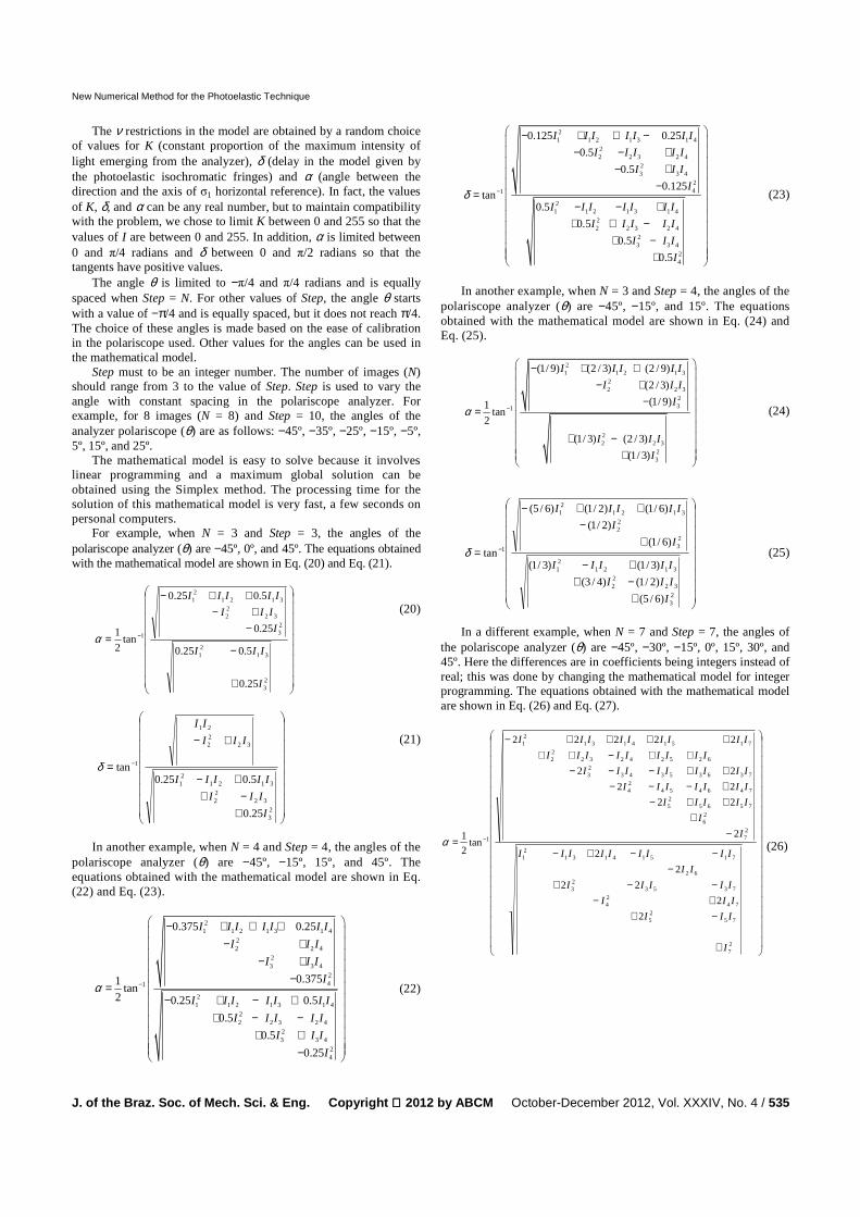
For example, when N = 3 and Step = 3, the angles of the polariscope analyzer (θ) are −45º, 0º, and 45º. The equations obtained with the mathematical model are shown in Eq. (20) and Eq. (21).

+

−

−+−

++−

= −

23

3121

23

3222

312121

1

25.0

5.025.0

25.0

5.025.0

tan2

1

I

III

I

III

IIIII

α

(20)

+−+

+−

+−

= −

23

3222

312121

3222

21

1

25.0

5.025.0tan

I

III

IIIII

III

II

δ

(21)

In another example, when N = 4 and Step = 4, the angles of the

polariscope analyzer (θ) are −45º, −15º, 15º, and 45º. The equations obtained with the mathematical model are shown in Eq. (22) and Eq. (23).

21 1 2 1 3 1 4

22 2 4

23 3 4

241

21 1 2 1 3 1 4

22 2 3 2 4

23 3 4

24

0.375 0.25

0.3751tan

2 0.25 0.5

0.5

0.5

0.25

I I I I I I I

I I I

I I I

I

I I I I I I I

I I I I I

I I I

I

α −

− + + +

− + − + −

= − + − + + − − + + −

(22)

21 1 2 1 3 1 4

22 2 3 2 4

23 3 4

241

21 1 2 1 3 1 4

22 2 3 2 4

23 3 4

24

0.125 0.25

0.5

0.5

0.125tan

0.5

0.5

0.5

0.5

I I I I I I I

I I I I I

I I I

I

I I I I I I I

I I I I I

I I I

I

δ −

− + + −

− − + − + −

= − − + + + − + − +

(23)

In another example, when N = 3 and Step = 4, the angles of the

polariscope analyzer (θ) are −45º, −15º, and 15º. The equations obtained with the mathematical model are shown in Eq. (24) and Eq. (25).

21 1 2 1 3

22 2 3

231

22 2 3

23

(1/ 9) (2 / 3) (2 / 9)

(2 /3)

(1/ 9)1tan

2

(1/ 3) (2 / 3)

(1/ 3)

I I I I I

I I I

I

I I I

I

α −

− + +

− + − = + − +

(24)

+−++−

+−

++−

= −

23

3222

312121

23

22

312121

1

)6/5(

)2/1()4/3(

)3/1()3/1(

)6/1(

)2/1(

)6/1()2/1()6/5(

tan

I

III

IIIII

I

I

IIIII

δ

(25)

In a different example, when N = 7 and Step = 7, the angles of

the polariscope analyzer (θ) are −45º, −30º, −15º, 0º, 15º, 30º, and 45º. Here the differences are in coefficients being integers instead of real; this was done by changing the mathematical model for integer programming. The equations obtained with the mathematical model are shown in Eq. (26) and Eq. (27).

+

−++−−−+

−−−+−

−+

++−+−−−++−−−

++−++++++−

= −

27

7525

7424

735323

62

7151413121

27

26

756525

74645424

7363534323

6252423222

7151413121

1

2

2

22

2

2

2

22

22

22

22222

tan2

1

I

III

III

IIIII

II

IIIIIIIII

I

I

IIIII

IIIIIII

IIIIIIIII

IIIIIIIII

IIIIIIIII

α

(26)

Júnior et al.


+−

−+−+−+

+−+−−−

−+++−

−−+−+−+−++++−

= −

27

26

7525

7424

7323

6222

7151413121

27

7626

7525

6424

7323

724222

716151312121

1

2

22

22

22

2

22222

2

22

22

2

22

222

222222

tan

I

I

III

III

III

III

IIIIIIIII

I

III

III

III

III

IIIII

IIIIIIIIIII

δ (27)

For example, with 10 images (N = 10) and Step = 10, the angles of the analyzer polariscope (θ) are as follows (∆θ = 10º): θ1 = −45º, θ2 = −35º, θ3 = −25º, θ4 = −15º, θ5 = −5º, θ6 = 5º, θ7 = 15º, θ8 = 25º, θ9 = 35º, and θ10 = 45º. The equations obtained with the mathematical model are shown in Table 1 with values of the coefficients (br,s, cr,s, er,s, fr,s).

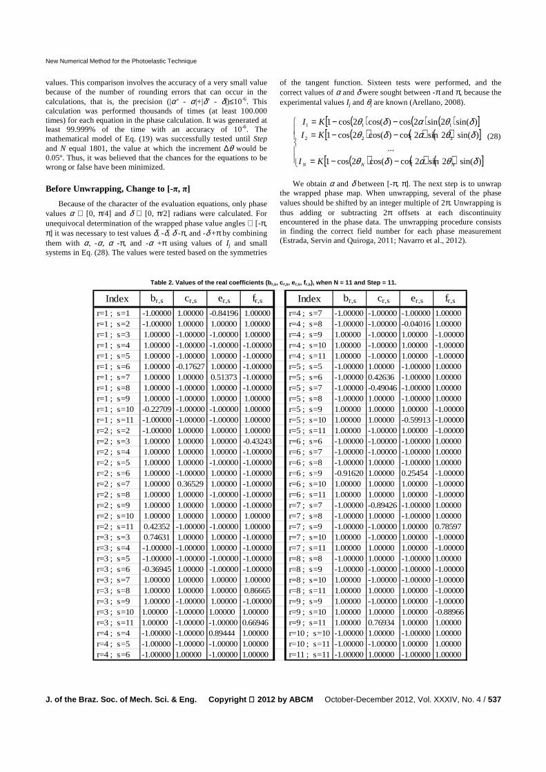
For example, with N = 11 and Step = 11, the angles of the analyzer polariscope (θ) are as follows (∆θ = 9º): θ1 = −45º, θ2 = −36º, θ3 = −27º, θ4 = −18º, θ5 = −9º, θ6 = 0º, θ7 = 9º, θ8 = 18º, θ9 = 27º, θ10 = 36º, and θ11 = 45º. The equations obtained with the mathematical model are shown in Table 2 with values of the coefficients (br,s, cr,s, er,s, fr,s). The coefficients are displayed with 5 decimal places, but were calculated in 19 decimal places of accuracy. These values are shown for purposes of direct use of the new equations and conference implementation of the mathematical model.

Table 1. Values of the real coefficients ( br,s, cr,s, er,s, fr,s), when N = 10 and Step = 10.

Thus, for each value of Step greater than or equal to 3 and N between 3 and the value of Step, the mathematical model of Eq. 19 provides values of the real coefficients (br,s, cr,s, er,s, fr,s), which represents an unprecedented and new phase equation for α and δ.

Because the new equations were developed from the algorithms, a numerical calculation, rather than an analytical demonstration of trigonometric relations, is necessary to check them. It is believed that a large number of numerical tests can validate or verify these new equations or at least minimize the chance of these equations being wrong or false. To test the usefulness of the new equations for

calculating the phase, a computer program was created, which generated random values of K∈[0, 255], α’∈[0, π/4], and δ’∈[0, π/2]. Using Eq. (3), the program calculates N values of I j, one for each value of θj. With the values of I j, the new phase equations were applied and tested to determine whether they produced the correct values of α and δ. The values of I j (luminous intensity of the image) are calculated with j ranging from 1 to N. The new equations with the values of I j are applied, giving a tan (α) and a tan (δ) that must be compared with the value of randomly assigned (α’ and δ’ )

Index br,s cr,s er,s fr,s Index br,s cr,s er,s fr,s r=1 ; s=1 -1.00000 -1.00000 -1.00000 1.00000 r=4 ; s=4 -1.00000 -1.00000 -1.00000 1.00000 r=1 ; s=2 -1.00000 1.00000 -0.87367 1.00000 r=4 ; s=5 -1.00000 -1.00000 -1.00000 1.00000 r=1 ; s=3 1.00000 1.00000 1.00000 0.91797 r=4 ; s=6 -1.00000 -1.00000 -1.00000 1.00000 r=1 ; s=4 1.00000 1.00000 1.00000 -1.00000 r=4 ; s=7-1.00000 1.00000 -1.00000 1.00000 r=1 ; s=5 1.00000 1.00000 1.00000 -1.00000 r=4 ; s=8-0.03206 -1.00000 1.00000 1.00000 r=1 ; s=6 1.00000 -1.00000 -1.00000 -1.00000 r=4 ; s=9 1.00000 -1.00000 1.00000 -1.00000 r=1 ; s=7 1.00000 1.00000 1.00000 -1.00000 r=4 ; s=10 1.00000 -1.00000 -0.35622 -1.00000 r=1 ; s=8 1.00000 -0.12390 1.00000 1.00000 r=5 ; s=5-1.00000 -1.00000 -1.00000 1.00000 r=1 ; s=9 0.56382 -1.00000 1.00000 1.00000 r=5 ; s=6-1.00000 1.00000 -1.00000 1.00000 r=1 ; s=10 -1.00000 -1.00000 -1.00000 1.00000 r=5 ; s=7 -1.00000 1.00000 -1.00000 1.00000 r=2 ; s=2 -0.87625 0.72262 1.00000 1.00000 r=5 ; s=8-1.00000 -0.84173 0.29954 -1.00000 r=2 ; s=3 1.00000 1.00000 1.00000 -1.00000 r=5 ; s=91.00000 1.00000 1.00000 -1.00000 r=2 ; s=4 1.00000 -1.00000 1.00000 -1.00000 r=5 ; s=10 1.00000 -1.00000 1.00000 -1.00000 r=2 ; s=5 1.00000 -1.00000 1.00000 -1.00000 r=6 ; s=6 -1.00000 1.00000 -1.00000 1.00000 r=2 ; s=6 1.00000 -1.00000 -1.00000 -1.00000 r=6 ; s=7 -1.00000 -1.00000 -1.00000 1.00000 r=2 ; s=7 1.00000 1.00000 1.00000 -1.00000 r=6 ; s=8-1.00000 -1.00000 1.00000 -0.95811 r=2 ; s=8 1.00000 -1.00000 1.00000 -1.00000 r=6 ; s=9 1.00000 -0.75947 1.00000 -1.00000 r=2 ; s=9 1.00000 -1.00000 1.00000 1.00000 r=6 ; s=10 1.00000 -1.00000 1.00000 -1.00000 r=2 ; s=10 1.00000 1.00000 -1.00000 1.00000 r=7 ; s=7 -1.00000 1.00000 -1.00000 1.00000 r=3 ; s=3 1.00000 1.00000 1.00000 -1.00000 r=7 ; s=8-1.00000 1.00000 1.00000 1.00000 r=3 ; s=4 -1.00000 1.00000 0.61212 -1.00000 r=7 ; s=9 1.00000 1.00000 1.00000 -1.00000 r=3 ; s=5 -1.00000 -1.00000 -1.00000 -1.00000 r=7 ; s=10 1.00000 1.00000 1.00000 -1.00000 r=3 ; s=6 -1.00000 -0.67863 -1.00000 0.42187 r=8 ; s=8 1.00000 1.00000 -0.84213 0.35815 r=3 ; s=7 0.52638 1.00000 -1.00000 1.00000 r=8 ; s=91.00000 0.68111 -1.00000 -1.00000 r=3 ; s=8 1.00000 1.00000 1.00000 1.00000 r=8 ; s=101.00000 -1.00000 1.00000 -1.00000 r=3 ; s=9 1.00000 1.00000 1.00000 -0.73988 r=9 ; s=9-0.81120 1.00000 -1.00000 1.00000 r=3 ; s=10 1.00000 -1.00000 -1.00000 -1.00000 r=9 ; s=10 -1.00000 -1.00000 1.00000 1.00000

r=10 ; s=10 -1.00000 1.00000 -0.61617 1.00000



values. This comparison involves the accuracy of a very small value because of the number of rounding errors that can occur in the calculations, that is, the precision (|α’ - α|+|δ’ - δ|)≤10-6. This calculation was performed thousands of times (at least 100.000 times) for each equation in the phase calculation. It was generated at least 99.999% of the time with an accuracy of 10-6. The mathematical model of Eq. (19) was successfully tested until Step and N equal 1801, the value at which the increment ∆θ would be 0.05º. Thus, it was believed that the chances for the equations to be wrong or false have been minimized.

Before Unwrapping, Change to [-π, π]

Because of the character of the evaluation equations, only phase values α ∈ [0, π/4] and δ ∈ [0, π/2] radians were calculated. For unequivocal determination of the wrapped phase value angles ∈ [-π, π] it was necessary to test values δ, -δ, δ -π, and -δ +π by combining them with α, -α, α -π, and -α +π using values of I j and small systems in Eq. (28). The values were tested based on the symmetries

of the tangent function. Sixteen tests were performed, and the correct values of α and δ were sought between -π and π, because the experimental values I j and θj are known (Arellano, 2008).

( ) ( ) ( )[ ]( ) ( ) ( )[ ]

( ) ( ) ( )[ ]

−−=

−−=−−=

)sin(2sin2cos)cos(2cos1

...



222

111

δθαδθ

δθαδθδθαδθ

NNN KI

KI

KI

(28)

We obtain α and δ between [-π, π]. The next step is to unwrap

the wrapped phase map. When unwrapping, several of the phase values should be shifted by an integer multiple of 2π. Unwrapping is thus adding or subtracting 2π offsets at each discontinuity encountered in the phase data. The unwrapping procedure consists in finding the correct field number for each phase measurement (Estrada, Servin and Quiroga, 2011; Navarro et al., 2012).

Table 2. Values of the real coefficients ( br,s, cr,s, er,s, fr,s), when N = 11 and Step = 11.

Index br,s cr,s er,s fr,s Index br,s cr,s er,s fr,s r=1 ; s=1 -1.00000 1.00000 -0.84196 1.00000 r=4 ; s=7 -1.00000 -1.00000 -1.00000 1.00000 r=1 ; s=2 -1.00000 1.00000 1.00000 1.00000 r=4 ; s=8-1.00000 -1.00000 -0.04016 1.00000 r=1 ; s=3 1.00000 -1.00000 -1.00000 1.00000 r=4 ; s=9 1.00000 -1.00000 1.00000 -1.00000 r=1 ; s=4 1.00000 -1.00000 -1.00000 -1.00000 r=4 ; s=10 1.00000 -1.00000 1.00000 -1.00000 r=1 ; s=5 1.00000 -1.00000 1.00000 -1.00000 r=4 ; s=11 1.00000 -1.00000 1.00000 -1.00000 r=1 ; s=6 1.00000 -0.17627 1.00000 -1.00000 r=5 ; s=5 -1.00000 1.00000 -1.00000 1.00000 r=1 ; s=7 1.00000 1.00000 0.51373 -1.00000 r=5 ; s=6-1.00000 0.42636 -1.00000 1.00000 r=1 ; s=8 1.00000 -1.00000 1.00000 -1.00000 r=5 ; s=7 -1.00000 -0.49046 -1.00000 1.00000 r=1 ; s=9 1.00000 -1.00000 1.00000 1.00000 r=5 ; s=8-1.00000 1.00000 -1.00000 1.00000 r=1 ; s=10 -0.22709 -1.00000 -1.00000 1.00000 r=5 ; s=9 1.00000 1.00000 1.00000 -1.00000 r=1 ; s=11 -1.00000 -1.00000 -1.00000 1.00000 r=5 ; s=10 1.00000 1.00000 -0.59913 -1.00000 r=2 ; s=2 -1.00000 1.00000 1.00000 1.00000 r=5 ; s=11 1.00000 -1.00000 1.00000 -1.00000 r=2 ; s=3 1.00000 1.00000 1.00000 -0.43243 r=6 ; s=6-1.00000 -1.00000 -1.00000 1.00000 r=2 ; s=4 1.00000 1.00000 1.00000 -1.00000 r=6 ; s=7-1.00000 -1.00000 -1.00000 1.00000 r=2 ; s=5 1.00000 1.00000 -1.00000 -1.00000 r=6 ; s=8 -1.00000 1.00000 -1.00000 1.00000 r=2 ; s=6 1.00000 -1.00000 1.00000 -1.00000 r=6 ; s=9 -0.91620 1.00000 0.25454 -1.00000 r=2 ; s=7 1.00000 0.36529 1.00000 -1.00000 r=6 ; s=10 1.00000 1.00000 1.00000 -1.00000 r=2 ; s=8 1.00000 1.00000 -1.00000 -1.00000 r=6 ; s=11 1.00000 1.00000 1.00000 -1.00000 r=2 ; s=9 1.00000 1.00000 1.00000 -1.00000 r=7 ; s=7-1.00000 -0.89426 -1.00000 1.00000 r=2 ; s=10 1.00000 1.00000 1.00000 1.00000 r=7 ; s=8-1.00000 1.00000 -1.00000 1.00000 r=2 ; s=11 0.42352 -1.00000 -1.00000 1.00000 r=7 ; s=9 -1.00000 -1.00000 1.00000 0.78597 r=3 ; s=3 0.74631 1.00000 1.00000 -1.00000 r=7 ; s=10 1.00000 -1.00000 1.00000 -1.00000 r=3 ; s=4 -1.00000 -1.00000 1.00000 -1.00000 r=7 ; s=11 1.00000 1.00000 1.00000 -1.00000 r=3 ; s=5 -1.00000 -1.00000 -1.00000 -1.00000 r=8 ; s=8 -1.00000 1.00000 -1.00000 1.00000 r=3 ; s=6 -0.36945 1.00000 -1.00000 -1.00000 r=8 ; s=9 -1.00000 -1.00000 -1.00000 -1.00000 r=3 ; s=7 1.00000 1.00000 1.00000 1.00000 r=8 ; s=101.00000 -1.00000 -1.00000 -1.00000 r=3 ; s=8 1.00000 1.00000 1.00000 0.86665 r=8 ; s=111.00000 1.00000 1.00000 -1.00000 r=3 ; s=9 1.00000 -1.00000 1.00000 -1.00000 r=9 ; s=9 1.00000 -1.00000 1.00000 -1.00000 r=3 ; s=10 1.00000 -1.00000 1.00000 1.00000 r=9 ; s=10 1.00000 1.00000 1.00000 -0.88966 r=3 ; s=11 1.00000 -1.00000 -1.00000 0.66946 r=9 ; s=11 1.00000 0.76934 1.00000 1.00000 r=4 ; s=4 -1.00000 -1.00000 0.89444 1.00000 r=10 ; s=10 -1.00000 1.00000 -1.00000 1.00000 r=4 ; s=5 -1.00000 -1.00000 -1.00000 1.00000 r=10 ; s=11 -1.00000 -1.00000 1.00000 1.00000 r=4 ; s=6 -1.00000 1.00000 -1.00000 1.00000 r=11 ; s=11 -1.00000 1.00000 -1.00000 1.00000

Júnior et al.


Testing and Analysis of Error

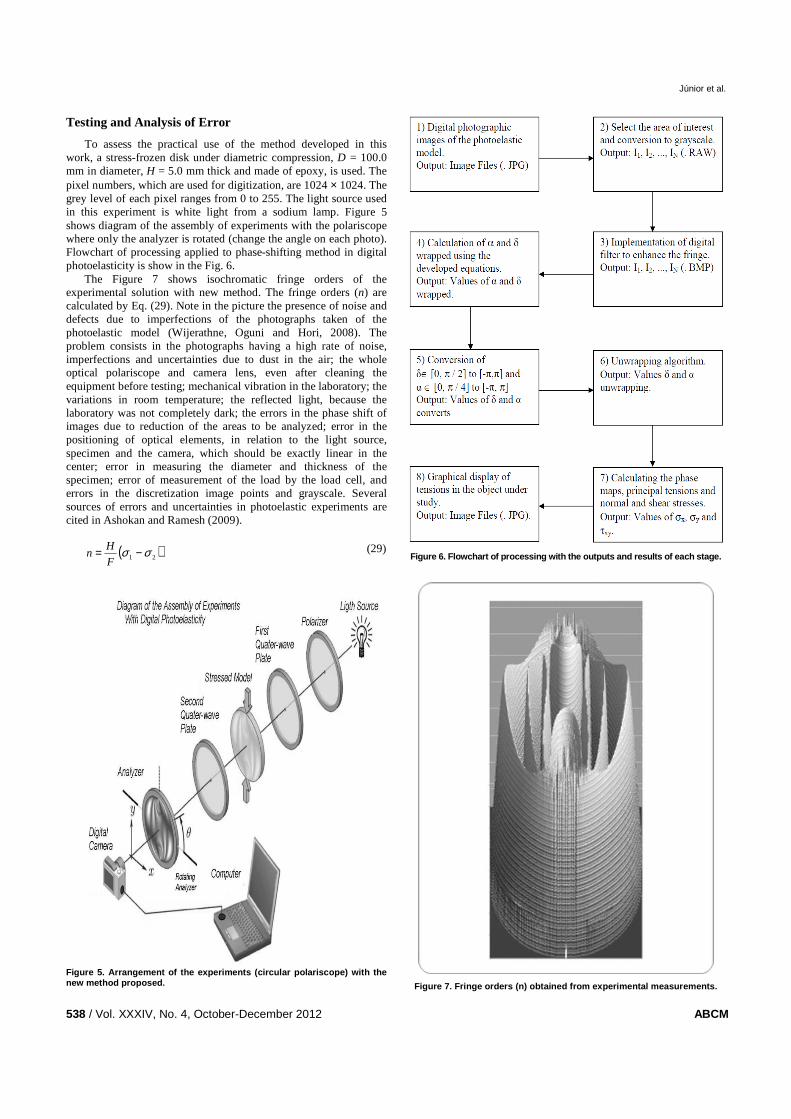
To assess the practical use of the method developed in this work, a stress-frozen disk under diametric compression, D = 100.0 mm in diameter, H = 5.0 mm thick and made of epoxy, is used. The pixel numbers, which are used for digitization, are 1024 × 1024. The grey level of each pixel ranges from 0 to 255. The light source used in this experiment is white light from a sodium lamp. Figure 5 shows diagram of the assembly of experiments with the polariscope where only the analyzer is rotated (change the angle on each photo). Flowchart of processing applied to phase-shifting method in digital photoelasticity is show in the Fig. 6.

The Figure 7 shows isochromatic fringe orders of the experimental solution with new method. The fringe orders (n) are calculated by Eq. (29). Note in the picture the presence of noise and defects due to imperfections of the photographs taken of the photoelastic model (Wijerathne, Oguni and Hori, 2008). The problem consists in the photographs having a high rate of noise, imperfections and uncertainties due to dust in the air; the whole optical polariscope and camera lens, even after cleaning the equipment before testing; mechanical vibration in the laboratory; the variations in room temperature; the reflected light, because the laboratory was not completely dark; the errors in the phase shift of images due to reduction of the areas to be analyzed; error in the positioning of optical elements, in relation to the light source, specimen and the camera, which should be exactly linear in the center; error in measuring the diameter and thickness of the specimen; error of measurement of the load by the load cell, and errors in the discretization image points and grayscale. Several sources of errors and uncertainties in photoelastic experiments are cited in Ashokan and Ramesh (2009).

( )21 σσ −=F

Hn (29)

Figure 5. Arrangement of the experiments (circular polariscope) with the new method proposed.

Figure 6. Flowchart of processing with the outputs and results of each stage.

Figure 7. Fringe orders ( n) obtained from experimental measurements.



To test the new equations for the phase calculation, they were

used with the technique of photoelasticity for an object with known stress and to evaluate the average error using Eq. (30) and Eq. (31). This process was started with three images, repeated with four, then five and so on. The idea was to show that with an increasing number of images, the average error tends to decrease. Figure 8 shows an example of this procedure.

Figure 8. Set with 6 images of the photographs take n of the photoelastic model, ∆∆∆∆θθθθ equal to 18°, the disk is under compression.

1

1 ( )

Mei i

i

Average Error for EMαα α α

=

= −∑ (30)

1

1 ( )

Mei i

i

Average Error for EMδδ δ δ

=

= −∑ (31)

where M is the number of pixels of the image and αi

e and δie are the

exact values calculated by Eqs. (6)-(12) for the disk. The values of αi and δi are calculated by the new equation. In the analysis of the error, only the zones within the photos that were unambiguous and contained no inconsistencies were considered (Ashokan and Ramesh, 2009).

To compare the new equations for calculating the phase, nine sets of photos with Step set to 3, 4, 6, 7, 10, 11, 16, 19, and 31 were generated. In each set, the angle θ of the analyzer is varied (∆θ): 45º, 30º, 18º, 15º, 10º, 9º, 6º, 5º, and 3º, respectively. Each set was computed using the average error of 3 to the number of Step images and using equations to evaluate the angles α and δ. The data are shown below in Tables 3 and 4. Figures 9 and 10 show that the average error decreases when the number of images increases. It may be noted that for a number of images, the average error increases when the variation of the angle θ between the images decreases.

It is important to note that for each equation developed, the average errors found for the angle δ are larger than the errors found for the angle α of the fringes isoclines. It is believed that this occurs because the absolute values of δ are higher than the absolute values of α.

Table 3. Average error in 10 -6 rad versus number of frames ( N) for angle �.

Figure 9. A plot of the data from Table 3 with the average error in 10 -6 rad versus the number of frames ( N) for angle αααα.

Set of

Image1 2 3 4 5 6 7 8 9

∆θ ∆θ ∆θ ∆θ 45º 30º 18º 15º 10º 9º 6º 5º 3º

Step 3 4 6 7 10 11 16 19 31

3 4712 6879 9762 11256 16786 18342 22312 27453 29601

4 4005 6239 9562 11076 16265 18003 22201 27298

5 3955 5945 8654 9698 12671 15643 18964

6 3520 3645 4521 4799 5210 7564 9863

7 3290 3489 3845 4075 6178 7843

8 3132 3320 3821 5854 6582

9 2985 3255 3594 5123 5987

10 2845 2930 3278 4021 4388

11 2602 2725 3267 3678

12 2503 3077 3333

13 2384 2988 3167

14 2241 2845 3011

15 2133 2458 2637

16 1921 2112 2353

17 1682 1976

18 1378 1734

19 1241 1667

20 1535

21 1402

22 1378

23 1320

24 1298

25 1204

26 1167

27 1076

28 1005

29 945

30 806

31 745

Nu

mb

er

of

Ima

ge

(N

)

Average

Error of

the αααα in

10-6

rad

Júnior et al.


Figure 10. A plot of the data from Table 4 with the average error in 10 -6 rad versus the number of frames ( N) for angle δδδδ.

Table 4. Average error in 10 -6 rad versus the number of frames ( N) for angle δδδδ.

Figure 11. Results obtained through experimental me asurements using the new equations with N = 6 and Step = 6 of: δδδδ, αααα, fringe order( n), σσσσ1, σσσσ2, von Mises stress( σσσσυυυυ), σσσσx, σσσσy and ττττxy.

To compare the present equations with the equations deduced

by other authors, the equations were applied to the analysis of error in the algorithm of Patterson and Wang (1991). Values of Eα = 2104 × 10-6 rad and Eδ = 5312 × 10-6 rad were obtained.

For the Patterson and Wang algorithm with six images, the average error is less than six images using the new equations. It is believed that the major distinction between the pictures of the phase shifts is the reason why this improved result is obtained. However, to obtain these images, it is necessary to rotate the analyzer and the second plate of the polariscope by a quarter-wave.

The average error of the algorithm of Wang and Patterson with 6 images is in the range of the average error found for 11 images using the new equations, but for more than 16 images, lower average errors for the newly developed equations can be observed, indicating that a larger number of images yielded smaller errors. Similar results were obtained with the algorithms proposed by other authors in Ramji and Prasath (2011), Ramji and Ramesh (2008) and Chang and Wu (2011).

The significant advantage of the methodology proposed in this paper is that the method only changes the angle of the analyzer in the polariscope and that one can obtain equations for calculating the phase for any number of images in various situations.

More experiments were performed with other values of load (P), diameter of the disk (D), the disk thickness (H), and material fringe constant (F) with very similar results. These new experiments were conducted to validate and confirm the proposed method.

Figures 11 and 12 show the results obtained with the application of the new phase calculation equations developed for various values of N and Step. Note that there is little visual or graphic difference between the results obtained using the three different equations. This is due to high resolution graphics of photographic images, and

Set of

image1 2 3 4 5 6 7 8 9

∆θ ∆θ ∆θ ∆θ 45º 30º 18º 15º 10º 9º 6º 5º 3º

Step 3 4 6 7 10 11 16 19 31

3 10577 15721 22985 28654 40250 42066 46327 47965 49443

4 9745 14383 22952 26124 39867 41233 46076 48346

5 9517 13469 20263 29838 31335 36435 46432

6 8259 8679 11108 14491 20801 24452 37333

7 8084 8473 9447 13012 19179 31055

8 7694 9057 10271 17332 25002

9 7301 7999 8780 12566 19710

10 6890 7035 8017 9881 12700

11 6293 6574 8007 9127

12 6155 7592 8180

13 5738 7356 7802

14 5476 6990 7412

15 5348 6039 6479

16 4866 5165 5781

17 4377 4852

18 3880 4261

19 3541 4032

20 3821

21 3442

22 3386

23 3240

24 3152

25 2958

26 2867

27 2644

28 2412

29 2366

30 1907

31 1717

Average

Error of

the δδδδ in

10-6

rad

Nu

mb

er

of

Ima

ge

(N

)



the good results achieved with the new equations developed in the research. Numerically, the equations with more images have less uncertainty and therefore, they are more accurate. Thus, there was obtained the best values of stress with number of images N = 31 and Step = 31, than using N = 6 and Step = 6.

Once obtained the value of α and δ unwrapping, apply digital implementation of the shear difference technique for whole field stress separation of 2-D problems of any geometry showed in Ramesh (2000) and Ramji and Ramesh (2008abc). Thus, it calculates the values of the phase maps, principal tensions (σ1, σ2) and normal (σx, σy) and shear (τxy) stresses. The von Mises stress or equivalent tensile stress (συ), a scalar stress value that can be computed, too. Thereafter, graphical displays of tensions in the object under study are shown.

Figure 12. Results obtained through experimental me asurements using the new equations with N = 31 and Step = 31 of: δδδδ, αααα, fringe order( n), σσσσ1, σσσσ2, von Mises stress( σσσσυυυυ), σσσσx, σσσσy and ττττxy.

Conclusion

This paper addresses the equations used for phase calculation measurements with images using phase shifting technique. The new equations are shown to be capable of processing the optical signal of photoelasticity. These techniques are very precise, easy to use, and low cost. On the basis of the performed error analysis, it can be concluded that the new equations are very good phase calculation algorithms. The metric analysis of the considered system demonstrated that its uncertainties of measurement depend on the frame period of the grid, on the resolution of photos in pixel and on the number of frames. However, the uncertainties involved in the measurement of the geometric parameters and the phase still require attention. In theory, if we have many frames, the measurement errors become very small. The measurement results obtained by the optical system demonstrate its industrial and engineering applications in experimental mechanics.

New numerical equations are deduced to calculate the directions of the tensions and delays (phase maps of the isoclines and isochromatic fringes) for the full-field image automatically, by programming the phase shift method in digital photoelasticity. With these new equations, a larger number of images phase shifted only by rotation of the analyzer can be used, and the gain can be calculated with lower uncertainties. Numerical methods were employed in an unprecedented way with the photoelastic technique to obtain a methodology for deriving the new equations. Until now, these equations were determined by algebraic and analytic methods.

With the new equations, it was possible to develop a photoelastic system that moves the analyzer of the polariscope at a constant speed while a camera takes many pictures at equal intervals of times, like a film. With this technique, the obtained measurements are more precise, and there are fewer uncertainties.

Digital photoelasticity is an important optical metrology follow-up for stress and strain analysis using full-field digital photographic images. Advances in digital image processing, data acquisition, procedures for pattern recognition and storage capacity enable use of the computer-aided technique in automation and facilitate improvement of the digital photoelastic technique. Photoelasticity has seen some renewed interest in the past few years with digital imaging, image processing and new methods becoming readily available. However, further research is needed to improve the accuracy, the precision and the automation of the photoelastic technique.

Acknowledgements

The authors thank the generous support from Pontificia Universidade Católica de Minas Gerais – PUCMINAS, Conselho Nacional de Desenvolvimento Científico e Tecnológico – CNPq, and Fundação de Amparo à Pesquisa de Minas Gerais – FAPEMIG.

References

Arellano, N.I.T., Zurita, G.R., Fabian, C.M. and Castillo, J.F.V., 2008, “Phase shifts in the Fourier spectra of phase gratings and phase grids: an application for one-shot phase-shifting interferometry”, Opt. Express, 16, pp. 19330-19341.

Ashokan, K. and Ramesh, K., 2009, “Finite element simulation of isoclinic and isochromatic phasemaps for use in digital photoelasticity”, Experimental Techniques, 33, pp. 38-44.

Asundi, A.K., 2002, “MATLAB for Photomechanics – A Primer”, Elsevier Science.

Asundi, A.K., Tong, L. and Boay, C.G., 2001, “Dynamic Phase-Shifting Photoelasticity”, Appl. Opt., 40, pp. 3654-3658.

Baek, T.H., Kim, M.S., Morimoto, Y. and Fujigaki, M., 2002, “Separation of isochromatics and isoclinics from photoelastic fringes in a circular disk by phase measuring technique”, KSME International Journal, Vol. 16, No. 2, pp. 175-181.

Chang, S.H. and Wu, H.H.P., 2011, “Improvement of digital photoelasticity based on camera response function”, Appl. Opt., 50, pp. 5263-5270.

Collett, E., 2005, “Field Guide to Polarization” (SPIE Vol. FG05), SPIE Publications, ISBN: 0819458686.

Corso, F.D., Bigoni, D. and Gei, M., 2008, “The stress concentration near a rigid line inclusion in a prestressed, elastic material. Part I: Full-field solution and asymptotics”, Journal of the Mechanics and Physics of Solids, Vol. 56, Issue 3, pp. 815-838.

Estrada, J.C., Servin, M. and Quiroga, J.A., 2011, “Noise robust linear dynamic system for phase unwrapping and smoothing”, Opt. Express, 19, pp. 5126-5133.

Fernandez, M.S.B., 2011, “Metrological study for the optimal selection of the photoelastic model in transmission photoelasticity”, Appl. Opt., 50, pp. 5721-5727.

Huang, M.J. and Sung P.C., 2010, “Regional phase unwrapping algorithm for photoelastic phase map”, Opt. Express, 18, pp. 1419-1429.

Júnior et al.


Kihara, T., 2007, “Phase unwrapping method for three-dimensional stress analysis by scattered-light photoelasticity with unpolarized light. 2. Experiment”, Appl. Opt., 46, pp. 6469-6475.

Magalhaes P.A.A., Neto, P.S. and Barcellos, C.S., 2011, “Analysis of Shadow Moire Technique With Phase Shifting Using Generalisation of Carre Method”, Strain, Vol. 47, Issue s1, pp. e555-e571, DOI: 10.1111/j.1475-1305.2009.00655.x.

Navarro, M.A., Estrada, J.C., Servin, M., Quiroga, J.A. and Vargas, J., 2012, “Fast two-dimensional simultaneous phase unwrapping and low-pass filtering”, Opt. Express, 20, pp. 2556-2561.

Ng, T.W., 1997, “Derivation of retardation phase in computer-aided photoelasticity by using carrier fringe phase shifting”, Appl. Opt., 36, pp. 8259-8263.

Oh, J.T. and Kim, S.W., 2003, “Polarization-sensitive optical coherence tomography for photoelasticity testing of glass/epoxy composites”, Opt. Express, 11, pp. 1669-1676.

Patterson, E.A. and Wang, Z.F., 1991, “Towards full field automated photoelastic analysis of complex components”, Strain, Vol. 27, Issue 2, pp. 49-5.

Pinit, P. and Umezaki, E., 2007, “Digitally whole-field analysis of isoclinic parameter in photoelasticity by four-step color phase shifting technique”, Optics and Laser in Engineering, Vol. 45, pp. 795-807.

Ramesh, K., 2000, “Digital photoelasticity: advanced techniques and applications”, Springer-Verlag, Berlin, Germany.

Ramji, M. and Ramesh, K., 2008a, “Whole field evaluation of stress components in digital photoelasticity—issues, implementation and application”, Opt. Lasers Eng., 46(3), pp. 257-271.

Ramji, M. and Ramesh, K., 2008b, “Stress separation in digital photoelasticity, Part A—photoelastic data unwrapping and smoothing”, J. Aerosp. Sci. Technol., 60(1), pp. 5-15.

Ramji, M. and Ramesh, K., 2008c, “Stress separation in digital photoelasticity, Part B—whole field evaluation of stress components”, J. Aerosp. Sci. Technol., 60(1), pp. 16-25.

Ramji, M. and Prasath, R.G.R., 2011, “Sensitivity of isoclinic data using various phase shifting techniques in digital photoelasticity towards generalized error sources”, Optics and Lasers in Engineering, Vol. 49, Issues 9-10, pp. 1153-1167.

Wijerathne, M.L.L., Oguni, K. and Hori, M., 2008, “Stress field tomography based on 3D photoelasticity”, Journal of the Mechanics and Physics of Solids, Vol. 56, Issue 3, pp. 1065-1085.

new numerical method for the photoelastic technique new ... · departamento de engenharia mecânica...

Documents