next-state equation generation for asynchronous sequential
TRANSCRIPT

Scholars' Mine Scholars' Mine
Masters Theses Student Theses and Dissertations
1970
Next-state equation generation for asynchronous sequential Next-state equation generation for asynchronous sequential
circuits - normal mode circuits - normal mode
Gregory Martin Bednar
Follow this and additional works at: https://scholarsmine.mst.edu/masters_theses
Part of the Electrical and Computer Engineering Commons
Department: Department:
Recommended Citation Recommended Citation Bednar, Gregory Martin, "Next-state equation generation for asynchronous sequential circuits - normal mode" (1970). Masters Theses. 5467. https://scholarsmine.mst.edu/masters_theses/5467
This thesis is brought to you by Scholars' Mine, a service of the Missouri S&T Library and Learning Resources. This work is protected by U. S. Copyright Law. Unauthorized use including reproduction for redistribution requires the permission of the copyright holder. For more information, please contact [email protected].

NEXT-STATE EQUATION GENERATION
FOR ASYNCHRONOUS SEQUENTIAL CIRCUITS - NORMAL MODE
BY
GREGORY MARTIN BEDNAR, 1944-
A THESIS
Presented to the Faculty of the Graduate School of the
UNIVERSITY OF MISSOURI - ROLLA
In Partial Fulfillment of the Requirements for the Degree
MASTER OF SCIENCE IN ELECTRICAL ENGINEERING
1970
Approved by

ABSTRACT
This paper describes the known methods of generating
next-state equations for asynchronous sequential circuits
operating in normal fundamental mode. First, the methods
that have been previously developed by other authors are
explained and correlated in a simple and uniform language
in order that the subtle differences of these approaches
can be seen. This review is then followed by a develop-
ment of a new method for generating minimal next-state
equations which has some advantages over the previous
methods.
From the comparison of the previous known methods,
it is noted that any one of these methods may be desirable
for certain designs since each has some advantages that
the others do not have. However, these methods also have
limitations in that some methods can only be used with
particular types of assignments. Also, as flow tables
become larger the amount of work required to use some of
these methods becomes excessive and tedious.
The method developed here is a simple and straight
forward approach which can be used for any unicode, single
transition time assignment and will easily lend itself to
computer application. The heart of this method emanates
from the role that the Karnaugh map plays in the conven
tional approach for generating the next-state equations.
ii
iii
The main advantage of this method seems to be its capability
and proficiency in handling large flow tables.

iv
ACKNOWLEDGEMENT
The author wishes to express his appreciation and
extend his thanks to Dr. James H. Tracey for his assistance
and guidance throughout this project.
The author also wishes to express his gratitude to
his family for their interest and constant encouragement
rendered during the writing of this paper.

TABLE OF CONTENTS
ABSTRACT
ACKNOWLEDGEMENT
LIST OF ILLUSTRATIONS
I. INTRODUCTION
II. BASIC CONCEPTS AND TERMINOLOGY
A. Description of Asynchronous Sequential Circuits
1. 2. 3. 4. 5. 6. 7. 8.
9. 10.
Flow Table Fundamental Mode Normal Mode Internal State Assignment Transition Direct Transition Critical Race Uni-code Single Transition Time Assignment State Table Transition Table
B. Conventional Approach of Generating Next-State Equations
III. REVIEW OF THE KNOWN METHODS FOR GENERATING NEXT-STATE EQUATIONS
A. Method # 1- G. K. Maki, J. H. Tracey and R. J. Smith
B. Method # 2 - D. P. Burton and D. R. Noaks
c. Method # 3 - C. J. Tan
1. Basic Theory of Tan's Procedure 2. Tan's Specific Iterative
Procedure
v
Page
ii
iv
vii
1
3
3
5 6 6 7 7 7 7
8 8 8
9
14
14
28
46
47
58

IV. NEW METHOD OF GENERATING NEXT-STATE EQUATIONS
V. CONCLUSION
VI. BIBLIOGRAPHY
VII. VITA
vi
Page
76
94
101
102
Figure
1
2
3
4 (a)
4(b)
5
6
7
8
9
10
11
12
13
14
15
16 (a)
16(b)
17
18
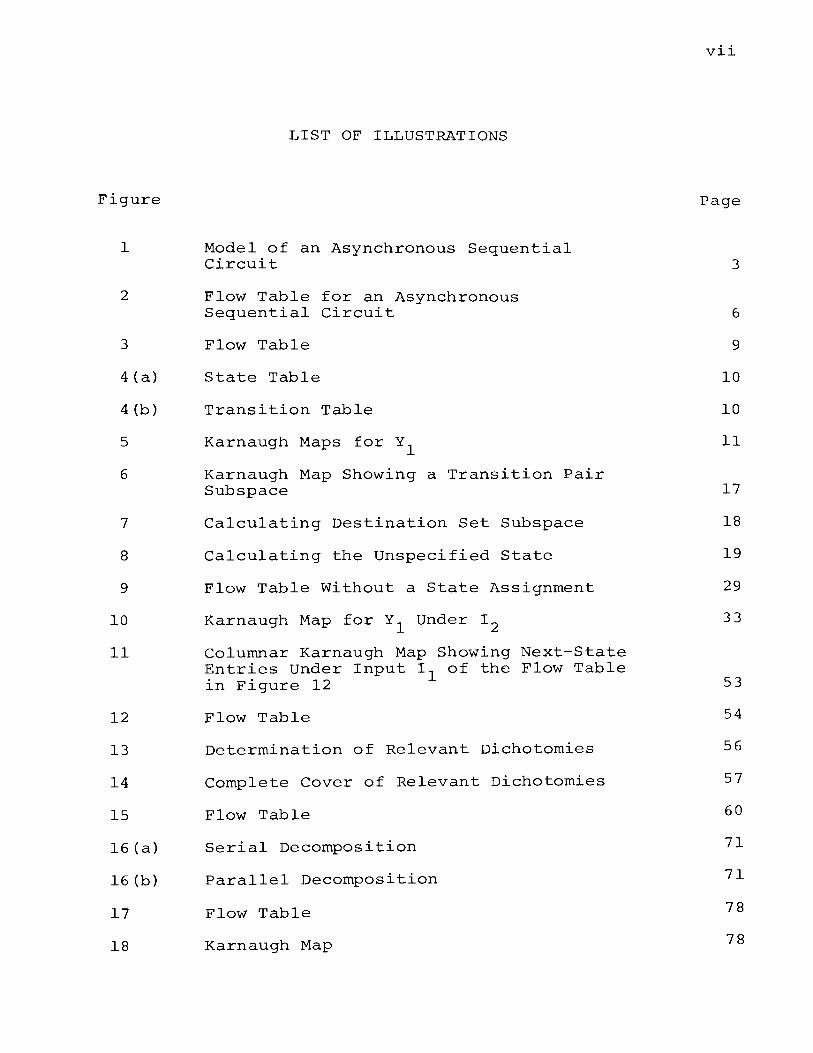
LIST OF ILLUSTRATIONS
Model of an Asynchronous Sequential Circuit
Flow Table for an Asynchronous Sequential Circuit
Flow Table
State Table
Transition Table
Karnaugh Maps for Y1
Karnaugh Map Showing a Transition Pair Subspace
Calculating Destination Set Subspace
Calculating the Unspecified State
Flow Table Without a State Assignment
Karnaugh Map for Y1 Under I 2
Columnar Karnaugh Map Showing Next-State Entries Under Input I 1 of the Flow Table in Figure 12
Flow Table
Determination of Relevant Dichotomies
Complete Cover of Relevant Dichotomies
Flow Table
Serial Decomposition
Parallel Decomposition
Flow Table
Karnaugh Map
vii
Page
3
6
9
10
10
11
17
18
19
29
33
53
54
56
57
60
71
71
78
78

I. INTRODUCTION
Sequential switching circuits are those circuits
whose operation and output depend on both the present and
previous inputs. These circuits can be further classified
into two categories called synchronous and asynchronous
sequential circuits. Synchronous circuits are those
circuits whose operation is timed or synchronized by
clock pulses. Conversely, asynchronous circuits are not
timed by clock pulses and offer the advantage of faster
operation, being limited only by the speed of the circuit
components involved in any particular operation.
In recent years, considerable work has been done in
the area of generating next-state equations for asynchro
nous sequential circuits. Although this work has been
accomplished by a number of people, it has been primarily
done on an individual basis without knowledge of each
other's efforts. The intent of this paper will be twofold.
First, the major works of other authors in this area will
be explained in a simple and uniform language so that the
subtle differences of these approaches can be seen and
correlated. Although the developments of the methods
presented here may differ somewhat from the original
presentations, the basic ideas of the credited authors
are used. Second, a development of a new method for
1

generating next-state equations will be given which has
advantages over the other methods.
The next section of this paper will review the basic
concepts of asynchronous sequential circuit theory. A
reader who is qualified in this area may skip this section.
2

II. BASIC CONCEPTS AND TERMINOLOGY
A. Description of Asynchronous Sequential Circuits
Asynchronous sequential circuits are usually repre-
sented by a block diagram of the type shown in Figure 1.
i
i Inputs
i
Present
State
Vari-
ables
1
2
p
0
0
0
yl
Y? . 0
y 0
Pure
Combinational
Logic
i Delay I I .
0
• I Delay I I
J Delay I L I
Outputs
{ Delay I _9
I 1
J 1 Delay I
0 0
0
{Delay I J
yl
Y,.., 0
0
- Next 0 y
n Stat e
Vari ables
3
Figure 1. Model of an Asynchronous Sequential Circuit
The delay shown in Figure 1 is the time required for the
signals to propagate through the combinational logic and
is inherent in the physical circuit components. Since pure
combinational logic (i.e., logic with no delay) can be
represented mathematically by Boolean algebra in the form
of output and next-state equations, the delay is considered

4
to be removed from the logic and lumped separately as shown.
In a simple mathematical model of an asynchronous circuit,
the delay associated with the output logic is ignored
while the delay of the next-state logic must be kept,
since it is part of a required feedback loop. It is this
lumped delay in the feedback loop that provides the
interpretation or physical distinction between the next
state and present-state variables. The value of the next
state variable will become the present state after some
delay in time.
Attention will now be directed toward obtaining the
next-state equations for the model shown in Figure 1. If
there are n internal-state variables and m input states
for such a model, the general form for the next state
equations will be:
Yl = fll(yl,y2,···,yn)Il + fli(yl,y2,···,yn)I2 +
+ flm(yl,y2,···,yn)Im
Y 2 = f 21. ( Y 1 'Y 2 ' • • • 'Y n) I 1 + f 2 2 ( Y 1 'Y 2 ' · • • 'Y n) I 2 + • • •
+ f2m(yl,y2,···,yn)Im
Yn = fnl(yl,y2,···,yn)Il + fn2(yl,y2,··· ,yn) 1 2 +
+ fnm(yl,y2,···,yn)Im ( 1)

where y 1 ,y 2 ,···,yn are the present state varia~les;
Y1 , Y2 , ···, Yn are the next-state variables; r1
, r2
,
Im are the input states; and f 11 , f 12 ,
tions of the internal-state variables.
f are funcnm
From hereafter
the next-state equations will be written in this form.
In this paper, minimization of these equations will be
done with respect to the function of the internal-state
variables only and will not consider codings of the input
states.
General information on this class of circuits can be
found in references [1] and [2].
1. Flow Table
The flow table is one of the principal means of
describing the operation of an asynchronous sequential
circuit. As shown in Figure 2, it is a two-dimensional
array consisting of next-state entries, with its columns
representing the input states and its rows representing
the internal states of the circuit. (The flow table
usually shows the output states, too, but in this paper
the output states are not relevant and therefore will
not be shown in the flow table.) The row in which the
circuit is currently operating is often referred to as the
present internal state or just the present state. For
example, if the present state of the circuit described by
Figure 2 is c and then an input of r 2 is applied, the next
state or state that the circuit will go to is e.
5

6
Il I2 Input States
a c 0 Internal b c 0 States c 0 e
d 0 a
e d 8 Figure 2. Flow Table for an Asynchronous Sequential Circuit
If a next-state entry is found to be the same as
the internal state representing that row, then the internal
state is said to be stable with respect to that input
column and is denoted by a circled next-state entry.
Similarly, uncircled entries denote unstable internal
states.
2. Fundamental Mode
An asynchronous sequential circuit is said to be
operating in fundamental mode if the inputs are never
changed unless the circuit is in a stable state.
3. Normal Mode
An asynchronous sequential circuit is said to be
operating in normal mode if each unstable state leads
directly to a stable state.

4. Internal-State Assignment
An internal-state assignment is a binary coding for
the internal states of a sequential circuit. For an
asynchronous circuit is must be constructed in a manner
such that the circuit will function according to flow
table specifications, independent of variations in trans
mission delays within the circuit.
5. Transition
The change of values of state variables from the
internal-state code associated with the present state to
the code associated with the next state is said to be a
transition from the present state to the next state.
6. Direct Transition
A transition whereby all state variables that are to
undergo a change of state are simultaneously excited is
direct transition.
7. Critical Race
A critical race is an undesirable feature of an
internal-state assignment which occurs when the binary code
of the next internal state differs from the code of the
present state in two or more bit positions, and there is
a possibility that unequal transmission delays may cause
the circuit to reach a stable state other than the one
intended.
7

8. Uni-code Single Transition Time Assignment
A state assignment is called a single transition
time (STT) assignment when all transitions are direct
transitions without critical races. Further, if only a
single coding is associated with each state, it is
called a uni-code single transition time (USTT)
assignment.
9. State Table
A state table differs from a flow table in that a
state table shows all of the internal states that a
sequential circuit can assume along with corresponding
next-state entries, whereas a flow table indicates only
the initial and final states. For example, a flow table
that has seven internal states and is coded with a four
variable internal-state assignment may have a correspond
ing state table with sixteen internal states. Of these
sixteen states, those which are not involved in any tran
sitions in the state table are referred to as the don't
care or unspecified states.
10. Transition Table
A transition table has the same form as the state
table except that the next-state entries are replaced with
their respective codes.
8

B. Conventional Approach of Generating Next-State Equations
Assume that the flow table with the USTT assignment
shown in Figure 3 describes the operation of a normal
fundamental mode asynchronous sequential circuit.
yl y2 y3 Il I2 I3
0 0 0 a 0 b 0 1 1 0 b c C0 C0 1 0 0 c 0 b a
0 0 1 d a 0 e
0 1 1 e 0 d 0 Figure 3. Flow Table
In using the conventional approach of generating the
next-state equations [1] it is necessary to first con-
struct the state and transition tables as shown in Fig-
ure 4. As previously mentioned, when constructing these
tables all possible internal-state codings must be listed
along with their corresponding next-state entries. Also
since all transitions must be direct and hence carried out
in a single transition time, it is necessary to insure
that no critical races can occur. Therefore, to prevent
a critical race during the transition from states a to b
under input I 2 , the intermediate state coded as 010 in the
state table must have state b as its next-state entry
under I 2 •
9

10
yl y2 y3 Il I2 I3
0 0 0 a 0 b G l l 0 b c @ ~ l 0 0 c 0 b a
0 0 l d a 0 e
0 l l e 0 d 0 0 l 0 b
l 0 l
l 1 1
(a)
yl y2 y3 Il I2 I3
0 0 0 a 8 110 ~ l 1 0 b 100 GB @ l 0 0 c ~ 110 000
0 0 1 d 000 G£Y 011
0 1 l e @ 001 @) 0 1 0 110
1 0 1
1 1 1
(b)
Figure 4. (a) State Table, (b) Transition Table
The next step is to construct Karnaugh maps from
the transition table and then derive the next-state

equations, Y. 's, where i represents the ith state variable. l
The Karnaugh maps for Y1 are shown in Figure 5.
Y1 under I 1 (denoted as Y1 , 1 )
0
1
00
0 - 1 0
0 0 ~ -Y1 under I 3
(denoted as Y1 , 3 )
Y1 under I 2 (denoted as Y1 , 2 )
Figure 5. Karnaugh Maps for Y1
By grouping the ones in the Karnaugh maps the sum-of-
products form of a Boolean expression for Y1 can be
derived:
yl = Yl,l + yl 2 + Yl,3 I
Yl,l = ylil
Yl,2 = y3I2
Yl,3 = yly2I3
Therefore,
11

Similarly, the equations for Y2 and Y3 are:
Definition: A y-variable expression is said to
cover a set of states if for those states the expression
is true (logical 1) and for all other states the expres
sion is false (logical 0).
This definition implies that the above next-state
equations cover those states whose corresponding next-
state variable, Y., has a value of one in some input l
column.
It would now be good to analyze the foregoing pro-
cedure to determine what has actually taken place and
why it works. The construction of the state and transi-
tion tables introduce the unspecified (or don't-care)
states which are later used in the Karnaugh maps to
obtain a reduced form of the next-state equations.
Another main point that should be noted from these tables
is that all states which lead to the same stable state
12
under a particular input have identical next-state entries.
This observation plays a prominent role in some of the
other procedures to be discussed later. Next, it is
observed that by using the Karnaugh map two important
feats are accomplished:

13
1) It permits the grouping of all ''1" next-state
variable entries into subcubes which can easily
be covered by subsets of internal-state variables.
These subcubes are the largest possible sub-
cubes which can be selected, such that they do
not contain any ''0" next-state variable entries.
(However, they may contain don't-care entries.)
Intuitively speaking, these groupings represent
the states involved in those transitions in
which the corresponding y-variable of the stable
state is one.
2) It provides a minimal y-variable expression that
covers those states which have a ''1" for their
Y. entry. l
This expression is formed from the
internal-state variables that cover the subcubes
obtained in 1) above.
Keeping these basic ideas in mind will provide
insight in the development of the more sophisticated methods
to be discussed later.
The main disadvantage of using the conventional
method to generate the next-state equations is the amount
of time needed to construct the state table, transition
table, and Karnaugh maps, especially for large flow tables.

III.
A. Method # l
REVIEW OF THE KNOWN METHODS FOR
GENERATING NEXT-STATE EQUATIONS
G. K. Maki, J. H. Tracey, and R. J. Smith
Maki, Tracey and Smith [3] jointly developed a means
to obtain the next-state equations directly from the flow
table and the internal state assignment. The advantage
of this method over the conventional approach is that the
state table, transition table, and Karnaugh maps do not
have to be explicitly formed.
Definition: A destination set of a flow table
column is the set of all unstable states leading to the
same stable state, together with that stable state.
This definition implies that a destination set is
a collection of all those states under a particular input
that have the same next-state entry.
for the flow table in Figure 3 are:
DI 1
a d
b c
e
DI 2
a b c
d e
The destination sets
14

where Dr. deontes the set of destination sets under input l
I. and the stable state of each destination set is l
underlined.
Definition: Each pair of states consisting of one
unstable state and the stable state of the destination
set is called a transition pair, since there is a transi-
tion from the unstable state to the stable state.
Note that a destination set may contain one or more
transition pairs. For example, the destination set a d
under r1
only contains one transition pair while the
destination set a b c under r 2 consists of two transition
pairs, a b and c b.
Definition: An internal state s is said to be an r
15
intermediate state between states s. and s. of a transition l J
pair if the state variables may assume the value associated
with the internal states during the transition from s. r 1
to s .. J
Definition: A transition pair subspace is a portion
of the total state space having a span that consists of
all possible internal states, both terminal and inter-
mediate, which can be assumed by the circuit during a
transition. This subspace is represented by a product
function of the internal state variables.

16
Consider the transition pair a b from the destination
set a b c under input I2
. The internal state coding for
states a and b are 0 0 0 and l l 0 respectively. During
the transition between states a and b, any of the internal
states 0, where the dashes represent all combinations
of l's and o•s, could be assumed momentarily due to
possible unequal transmission delays. To insure that the
circuit reaches the proper terminal state, all the states
represented by - - 0 must have the next-state entry of
l l o. It can be seen that this is the case in the transi-
tion table of Figure 4(b). These states form the transition
pair subspace which is expressed as y 3 .
The method developed by Maki, Tracey and Smith [3]
for representing the transition pair subspace as a product
of internal-state variables is as follows:
l) List the codes assigned to the states of the
transition pair.
2) The function that will represent the transition
pair subspace will be a product of the internal-
state variables. If the internal-state variable
y. is a l for both states of the transition pair, J
it will appear uncomplemented in the product
function. If the internal-state variable yj
appears as a 0 in both of the states of the
transition pair, its complement will appear in
the product function. If the internal-state
variable y. appears as both a l and a 0 in the J

states of the transition pair, it is considered
a don't-care variable and does not appear in the
product expression.
Therefore, using these rules, - - 0 is expressed as y3
.
The transition pair subspace is equivalent to the
subcube spanned by the transition pair in a Karnaugh map.
From the Karnaugh map of Figure 6, it is seen that the
transition a to b will take place within the subcube
covered by y 3 , where states 0 l 0 and l 0 0 could be inter-
mediate states of the transition. This agrees with the
result obtained earlier for the transition pair subspace.
00 01 11 10
0 (a - b c)
l d e - -
Figure 6. Karnaugh Map Showing a Transition Pair Subspace
17
Definition: A destination set subspace is that portion
of the total state space consisting of all possible internal
states that the circuit could assume during transitions
between states within the destination set.
The expression covering a destination set subspace
is equal to the sum of the transition pair subspaces, where
each transition pair subspace is represented as a product
of the internal-state variables. Using the destination set

18
a b c under input r 2 , Figure 7 shows the steps 1n finding
the destination set subspaces. Whereas the destination
set itself represented all terminal states of a flow table
Destination Transition Set Pairs
- --a b c a b ~
c b
Transition Destination Pair Sub spaces Set Subspace
- --~
0 - - or y3 ~ ~
1 0 ~ y3 + yly3 - or yly3
Figure 7. Calculating Destination Set Subspaces
column that have the same next-state entry, the destination
set subspaces represent all specified internal states of
a particular input column, both terminal and intermediate
states, that have the same next-state entry. Therefore,
destination set subspaces perform one of the functions
of the state table in the conventional approach since the
state table also designates all specified internal states.
Another main function of the state table, which will now
be considered, is the designation of all the unspecified
states (don't-cares) of the circuit. In order to obtain

19
the reduced form of the next-state equations, it is necessary
to use the unspecified states.
A sum-of-products expression which logically repre-
sents all the specified states of an input column can be
obtained by summing the expressions for the destination
set subspaces of that column. It then follows that the
unspecified states of that column would simply be the
logical complement of this expression. The simplified
expression for the unspecified states under input column r 2 is shown in Figure 8.
d e
Destination Set Sub spaces
Specified States under r 2
Unspecified States under r 2
Figure 8. Calculating the Unspecified States
The essential information contained in the state table of
the conventional approach is now available in the form of
logical y-variable expressions.
To find the next-state equation Y., only those groupl
ings of internal states which have a "l'' next-state entry
with respect toY. are considered. l
These groupings of
internal states correspond just to those destination set
subspaces in which the yi variable in the binary coding
for the stable state is a l. Again. this is true because
all next-state entries of the internal states represented

by the destination set subspaces are the same, namely that
of the stable state. So for example, if y 1 in the stable
state is 1, then all entries of the next-state variable
Y will be 1 for those states represented by the respec-1
tive destination set subspaces.
Definition: A destination set will be called a
1-destination set with respect to variable y. of y. = 1 l l
for the stable state and a a-destination set if y. = 0 ---- l
for the stable state.
To complete the construction of the next-state
equations it is only necessary to sum the logical expres-
sions representing the subspaces of those 1-destination
sets that are in the same input column along with the
expression representing the unspecified states of that
column. This will insure that the resulting next-state
expression representing that column will be in reduced
form after a simplification procedure is applied. Retain-
ing the identity of the input column with the simplified
expression, the process is then repeated for the remain-
ing input columns at which time the final equation will
be complete.
The process of combining the expressions represent-
ing the subspaces of the 1-destination sets with the
expressions representing the unspecified states of each
column is analogous to the function of the Karnaugh maps
20

in the conventional approach. With the Karnaugh map,
those states which had 1-entries for Y. were grouped with l
unspecified states in order to obtain the most minimal
form of the next-state expression.
To help provide a better understanding, a more
succinct picture of the foregoing method will be given by
first summarizing the steps of the procedure and then
following with an example.
1.
Maki-Smith-Tracey Procedure
List the destination sets
for each input column.
Meaning
Represents groupings of
internal states of flow
21
table that have same next-
state entries in a column.
2. Find y-variable expres- Equivalent to the subcube
sions for the transition of the Karnaugh map in
pair subspaces of each which the transition takes
destination set. place.
3. Form the y-variable Represents the groupings
expressions representing of the specified internal
the destination set sub- states in a state table
spaces by summing the which have the same next-
expressions representing state entries.
the transition pair sub-
spaces of each destination
set.

4. Find a y-variable expres
sion for the specified
states of each column by
summing the expressions
for all destination sets
subspaces in a column.
5. Find a y-variable expres
sion for the unspecified
states of each input
column by taking the
logical complement of the
expression representing
the specified states of
that column.
6.
7.
List the 1-destination
sets and their subspaces
for each input column.
Combine the expressions
representing the sub
spaces of the 1-destination
sets with the expression
representing the unspeci
fied states for each input
column to find the minimal
22
Steps 4 and 5 provide the
same information that is
found in the state table
of the conventional
approach.
Analogous to information
found in the transition
table and the Karnaugh
maps.
Equivalent to using
Karnaugh maps to find
minimal next-state expres
sions by selecting
groupings with maximum
1-entries and don't
cares.

23
form of next-state expres-
sions. Retain the identity
of each input state with
the resulting expression
for that column.
Example Problem
yl y2 y3 Il I2 I3
0 0 0 a 0 b 0 1 1 0 b c G G 1 0 0 c G b a
0 0 1 d a 0 e
0 1 1 e 0 d 0 The results of this method should be the same as the
results obtained in the conventional approach.
Following the steps of the above procedure:
1. The destination sets are:
DI 1
DI 2
DI 3
a d a b c a c
b c d e b -e d e
2. The transition pair subspaces are:

Input
Input
Destination Sets
a d
b c
e
a b c
d e
a c
b
d e
Transition Pairs
a d
b c
e
a b
b c
d e
a c
b
d e
Transition Pair Subspaces
0 0 - or y1y2
1 - 0 or y1y3
0 1 1 or Y1Y2Y3
- - 0 or y3
1 - 0 or y1y3
0 - 1 or y1y3
- 0 0 or y2y3
1 1 0 or y1y2y3
0 - 1 or y1y3
3. The destination set subspaces are:
Destination Sets Destination Set Subspaces
a d
b c
e
a b c
d e
a c
b
d e
24

25
4. Expressions for specified states of each input
column are:
Input Specified States
Note: The above expressions are not simplified.
5. Expressions for unspecified states of each column
after simplification are:
Input Unspecified States
6. The 1-destination sets and their subspaces are:
y-variable Input 1-Destination Sets Sub spaces
Il b c yly3 -
I2 a b c y3 + yly3
I3 b yly2y3

26
y-variable Input 1-Destination Sets Subs paces
e yly2y3 -
a b c y3 + yly3
b yly2y3
d e yly3 -
e yly2y3 -
d e yly3
d e yly3 -
7. Combining the subspaces for the 1-destination
sets with the expressions for the unspecified states yields
the following next-state equations:

y3 = [yly2y3 + d(yly3 + Y1Y2Y3) ]Il
+ [yly3 + d(yly3)]I2
+ [yly3 + d(yly3 + Y1Y2Y3) ]I3
where d( represents the subspaces of the unspecified
states. After simplifying:
yl = ylil + y3I2 + yly2I3
y2 = yly2Il + y3I2 + (y2 + y3)I3
y3 = Y1Y2I1 + y3I2 + Y3I3
When simplifying, only those don't-care states are used
which help simplify the next-state expressions. It is
seen that the equations obtained with this method are
identical to those of the conventional approach.
As mentioned earlier, the Maki, Tracey, and Smith
method generates a minimal set of next-state equations
without explicitly constructing the state and transition
tables. It sould also be pointed out that this method
will work for any satisfactory USTT assignment, i.e., no
matter whether the assignment has been developed from a
transition pair basis or a destination set basis. This
is true because transition pairs make up destination sets,
and this method uses transition pairs for its basic
building blocks as opposed to other methods that use
27

destination sets. Also, a computer program implementing
this method has been developed by Smith et al. [4].
B. Method # 2 D. P. Burton and D. R. Noaks
Burton and Noaks [5] recognized that for large flow
tables the derivation of next-state equations is a major
difficulty. The motivation for their method was to
establish a systematic procedure of obtaining a satis
factory USTT assignment for a normal-fundamental mode
flow table that would lead to relatively simple next-
state equations. The technique used to accomplish this
goal involves generating the next-state equations in a
semi-parallel fashion with the construction of the USTT
assignment. The next-state equations have the character
istics that no product terms contain more than one state
variable and no product terms contain any complemented
state variables.
Definition: A product term in the next-state equa-
tion is said to be a simple product term if it contains
only one internal-state variable.
Again, for correlation purposes, the same flow table
that was used in the previously discussed procedures will
be considered here and is repeated in Figure 9 for con-
venience.
unknown.
In this case, though, the USTT assignment is
28

Il I2 I3
a 0 b 0 b c ® ® c 0 b a
d a 0 e
e 0 d 0 Figure 9. Flow Table Without a State Assignment
As in the Maki, Tracey and Smith method, the first
step in this procedure is to list the destination sets
for each input column. In addition, associate with each
destination set an internal-state variable, y., such that l
y. = 1 for those states in the destination set and y. = 0 l l
for all other states. To help clarify the following
discussion, the destination sets associated with a y. l
state variable will sometimes be referred to as the y. l
destination set. The destination sets and associated
y-variables for the flow table in Figure 9 are:
DI 1
DI 2
DI 3
yl -+ {a d} y4 -+ {a b c} y6 -+ {a c}
y2 -+ {b c} Ys -+ {d e} y7 -+ {b}
y3 -+ {e} Ys -+ {d e}
29

30
This association of the state variables with the destination
sets provides the following initial USTT assignment for
the flow table:
yl y2 y3 y4 Ys y6 y7 Yg Internal States
1 0 0 1 0 1 0 0 a
0 1 0 1 0 0 1 0 b
0 1 0 1 0 1 0 0 c
1 0 0 0 1 0 0 1 d
0 1 1 0 1 0 0 1 e
In the previously ~iscussed methods, the next-state
equations consisted of y-variable expressions covering
those states ln which the next-state entries were 1. The
same is true in Burton and Noaks' method. From the above
assignment the next-state equations could be derived by
constructing the Karnaugh maps as in the conventional
approach, or by finding the expressions for the subspaces
of the 1-destination sets as in the Maki, Tracey and Smith
approach. But that would defeat the purpose of making a
larger assignment in the manner shown, sirtce it is supposed
to make thP construction of the next-state equations easier
than in the previous methods.
It was stated previously that in Burton and Noaks'
method each y. state variable will be a 1 for only those l
states in its associated y. destination set. l
Since all
next-state entries for the states in a destination set are

the same and equal to the stable state, the states of
those destination sets whose stable states are contained
in the y. destination will have y. = 1 for their next-l l
state entry. Therfore, to derive the next-state equation
for some Y. 1 the stable states of all destination sets l
are compared with the states in the y. destination set. l
If the stable state of some destination set, say the y. J
destination set, is also a member of the y. destination l
set, then theY. equation must include a simple produce l
term y.I 1 where I is the input under which they. J m m J
destination set is located. Of course, if more than one
destination set under the same input have their stable
states contained in the y. destination set, the resulting l
equation for Y. will contain more than one simple product l
term with the same input. For instance, theY. equation l
may contain two simple product terms like yjim + ykim
which equals (y. + yk) I . J m
To illustrate the above ideas, the next-state equa-
tion for y 1 will be derived. Since the y 1 destination set
is {ad}, Y1 will equal one for all states in destination
sets whose stable states are either "a" or "d". The
destination sets under each input column which satisfy
this condition are:
-+ {a d} -+ {d e} y -+ {a c} 6
31

Therefore, the next-state equation for Y1 can easily be
written as
As previously noted, this same expression could be
obtained using the conventional approach by finding the
largest groupings of 1-entries and don't cares in a
Karnaugh map, and with the Maki, Tracey and Smith method
32
by combining the expressions of the subspaces for the
1-destination sets with the expressions for the unspecified
states. But with such a large assignment these methods
would require an excessive amount of work. For example,
consider the derivation of the term y 5r 2 of the above
equation, when using the conventional approach. The
Karnaugh map for Y1 and input column r 2 , which would be
constructed from the transition table, is shown in Fig-
ure 10. By circling the largest possible subcubes of the
map which contains only "1" and don't-care entries, an
expression for Y1 under input r 2 can be obtained. As
illustrated in this case, all 1-entries can be grouped into
one subcube which is covered by the state variable y 5 .
Therefore, from the Karnaugh map we can write the expres
sion y5
r2
which agrees with the result obtained above.
This example also illustrates that the use of don't-care
states in the derivation of the y-variable expressions
is inherent in Burton and Noaks' method.

33
y1y2y3y4
or--i r--i 0 0.--i.--i 0 0 r--i r--i 0 0 r--i r--i 0 00 r--i" r--i r--ir--i 0 0 0 0 r--i r--i r--i r--i 0 0
Ys y6 y7 Ys 00 0 0 r--ir--ir--i r--ir--i r--i r--i" r--i 0 0 0 0 00 0 0 0 0 0 0.--i r--i r--i r--i r--i" r--i r--i r--i
0 0 0 0 - 0 - - 0 - - 0 - - - - 0 -0 0 0 1 - - - - - - - - - - - -0 0 1 1 - - - - - -0 0 1 0 0 - - - - 0 0 - - - - 0 -0 1 1 0 - 0 0 0 - - - - 0 -
0 1 1 1 - - - - - - -0 1 0 1 - - - - - - - - - - - -0 1 0 0 - 0 0 0 - - - - 0 -1 1 0 0 ~
1 1 0 1 - - - - - - - - - -1 1 1 1 - - - - - - - - - - - - - -1 1 1 0 - - - - - - - - - -1 0 1 0 - - - - - - - - - - - - - -1 0 1 1 - - - - - - - - - - - - - -1 0 0 1 1 1 - - - - - - 1 1
1 0 0 0 - - - - - - - - - -
Figure 10. Karnaugh Map for Y1 under r 2

The foregoing discussion explains the heart of
Burton and Noaks' method. The remaining portions of their
method deal with minimization techniques for eliminating
redundant y-variables from the initial assignment and for
simplifying the corresponding next-state equations. The
description of these techniques will be stated in a
narrative fashion with an informal plausible proof given.
A more rigorous mathematical presentation and proof can
be found in the reference cited [5].
Simplification Test I:
The first test which is applied to check for
redundancy involves examining all terms in the next-state
equations of the form (y. + y. +···)I . l J m
If the union of
the destination sets associated with the y-variables of
this term is equal to:
1) some other ys destination set, then the term
(y. + y. + •••)I is replaced by y I . l J m s m
2) the total state set (i.e., the set of all
internal states in the flow table) , then the
term (y. + y. + ···)I is replaced by 1 • I l J m m
or just I . m
The reasoning behind these rules can be explained in the
following manner:
1) If there exists the term (y. + y.)I ln a l J m
next-state equation and if this term is true
34

(logical 1), then either y. or y. is true. l J
This
implies that the circuit is operating in a state
of they. destination set or in a state in the l
35
y. destination set. J
If the union of they. andy. l J
2)
destination sets equal the y destination set, s
then all the states of y. andy. destination sets l J
are in the ys destination set too. Therefore,
whenever y. or y. is true, y will also be true l J s
and the term (y. + y.)I can be replaced by y I . 1 J m s m
If there exists the term (y. + y.)I and the 1 J m
union of they. andy. destination sets equal l J
the total state set, then the circuit will always
be operating in a state of the yi destination
set or in a state of they. destination set. J
This implies that either y. or y. will always l J
be true and therefore the expression (y. + y.) l J
can be replaced by the constant 1. (Note: in
the term (y. + y.)I both y. andy. could not 1 J m 1 J
be true at the same time since this would imply
that two destination sets under the same input
shared a common state which is the condition of
a critical race.) These ideas can be extended
to any term in the next-state equations of the
form (y. + y. + yk + •••)I . 1 J m
An example of Test I can be given by considering
the next-state equation for y 4 of the preceding assignment.

Remembering the method of derivation, the equation for y 4
can be written as:
It is observed that there are two compound terms in the
equation. First, looking at the term (yi + y2)I
1, the
union of the associated destination sets yields the set
{a b c d} which is not the same as any one destination set.
Therefore, the expression (y 1 + y 2 ) cannot be reduced.
Now looking at the other term (y 6 + y7)I 3 , the union of
the y 6 and y 7 destination sets yield the set {a b c}
which corresponds to the y 4 destination set. Therefore,
by Test I, the expression (y 6 + y7
) can be replaced by
y 4 . The reduced equation for Y4 is now:
Simplification Test II:
If two or more destination sets contain identical
states, whether or not they have the same stable state,
then these destination sets are referred to as being equiv
alent and the same y-variable can be assigned to both sets.
The reasoning behind this rule follows directly along the
same lines of Test I. If two different y-variables
represent equivalent destination sets, then both y-
variables will be true at the same time. Therefore, one
y-variable is redundant and can be eliminated. As an
36

37
example, the destination sets for the flow table in
Figure 9 will be considered. Under input I 2 , y 5 was
assigned to destination set (d e) and under input I3
, y8
was assigned to destination set (d e) . Since both of these
destination sets are equivalent (irrespective of which
states are stable), the y 8 variable can be eliminated and
the y 5 variable can be assigned to both destination sets.
This eliminates one y-variable of the initial assignment
and consequently one next-state equation.
Test II can also be restated in another way. If the
right hand side of two or more next-state equations are
identical, then only one of the y-variables associated with
the left hand side of these equations is necessary for the
assignment. This results from the fact that equivalent
destination sets will always give the same next-state
equations.
The next test in the minimization process is less
specific and clear-cut, but more important than the
previous tests. This test requires the construction of a
dependency diagram which is used to select a minimum set
of y-variables, from the remaining y-variables of the
initial assignment, that will provide a satisfactory USTT
assignment for the given flow table. Before listing the
steps of this test, it is necessary that a few fundamental
definitions and conditions for a satisfactory USTT assign
ment be stated.

Definition: A partition TI on a set of states is a
grouping of the states into disjoint subsets called
blocks, such that every state belongs to exactly one
block.
For example, a two-block partition may be defined
on the state set {abc de} as TI ={(abc), (de)}.
Definition: The smallest partition of a set of
states is denoted as TI(O} and corresponds to the parti-
tion in which each block consists of a single state.
From the preceding example, TI(O} ={(a} ,(b} ,(c},
(d},(e)}.
Definition: The blocks of a partition TI corresg
pending to the greater lower bound (g.l.b.} of partitions
Til and TI 2 , written as Til • TI 2 , consist of all the non
empty intersections that can be formed by intersecting a
block of Til with a block of TI 2 . The g.l.b. operation is
both commutative and associative.
For example, if
TI 1
= { (a b c} , ( d e} } and TI 2 = { (a b d} , ( c e} }
then
Tig =Til· TI 2 ={(a b},(c},(d),(e}}
Tracey [6] developed USTT assignment methods from
the idea that each binary valued state variable may be
thought of as inducing a two-block partition on the states
of a machine. Tracey [6] also proved in his Assignment
38

39
Method #2, that an USTT assignment will contain no critical
races if it has been made such that:
1) for every destination set D., if D. is another l J
destination set in the same input column, then
at least one y-variable partitions the destination
sets D. l
and D. J
into separate blocks.
2) all internal states are distinguished from one
another by being in separate blocks of at least
one y-variable partition.
Since these conditions lead to the formation of the
well-known Liu type assignment [7], they will be referred
to hereafter as the Liu assignment conditions. Using this
terminology will also help distinguish these conditions
from the conditions of the well-known Tracey assignment [6]
which will be discussed later.
It should be obvious that the initial assignment of
Burton and Noaks will satisfy the Liu assignment condi-
tions since a unique y-variable is assigned to each
destination set. A dependency diagram is then used to
show that a smaller set of the initial y-variable may exist
that also satisfies the Liu conditions which would, there-
fore, result in a smaller USTT assignment.
Simplification Test III:
This test involves the simplification of the state
assignment with the use of a dependency diagram. The rules
for the construction of dependency diagrams are:

1) Let each y-variable of the assignment represent
2)
a node of the diagram.
Check each y-variable's next-state equation.
the next-state variable, Y., is dependent on l
If
other y-variables draw arrows from the nodes of
the independent y-variables into the node of
the dependent next-state variable Y .. l
40
No formal procedure is known for selecting the minimum
set of state variables from the dependency diagram, and the
trial and error method suggested here differs somewhat from
the method presented by Burton and Noaks [5].
It is necessary to select a set of state variables
which have next-state equations independent of all other
state variables. This set can be found by drawing boundary
lines through the dependency diagram. These lines must be
constructed such that all arrows that pass through them
are in the same direction. Although the boundary lines
will separate sets of state variables which are independent
of the remaining variables, this does not, however, imply
that each set of independent variables will necessarily
result in a satisfactory assignment. To determine whether
the set of independent state variables selected do form a
satisfactory assignment, the two-block partitions induced
by these variables must satisfy the Liu assignment condi-
tions mentioned earlier. First, it is necessary to insure
that all destination sets under the same input are in

separate blocks of at least one y-variable partition, and
second, it is necessary to insure that all states are in
separate blocks of at least one y-variable partition. The
second condition will be satisfied if the g.l.b. of the
y-variable partisions is equal to n(O). If the Liu
assignment conditions do not hold, the next larger set of
independent y-variables is selected and tested. This
process is continued until a set of y-variables are
selected which will satisfy the Liu conditions. This set
of variables will result in the minimal Burton and Noaks'
assignment with corresponding minimal next-state equations.
This concludes the description of the Burton and
Noaks' method. A brief summary of the procedure is given
by the following steps:
1) List all destination sets of the flow table and
assign to each set a unique state variable.
2) Construct the next-state equations for the
initial state variables by using the strategy
of simple product terms.
3) Apply minimization techniques.
a) Test I - Replace compound terms with simpler
terms.
41
b) Test II - Eliminate redundant y-variables
that represent the same destination set.
(Note: This test may be applied concurrently
with Step 1.)

c) Test III - Construct and use the dependency
diagram.
The complete method will now be illustrated for the
flow table in Figure 9.
Step 1.
The destination sets and associated y-variables are
listed for each input column.
DI 1
DI 2
DI 3
yl -+ {a d} y4 -+ {a b c} y6 -+ {a c}
y2 -+ {b c} Ys -+ {d e} y7 -+ {b}
y3 -+ {e} Ys -+ {d e}
Minimization Test II was applied concurrently with this
step by assigning y 5 to two equal destination sets.
Step 2.
The set of next-state equations, written ln matrix
form for clarity, is:
42

yl yl Ys y6
y2 y2 y4 y7
YJ y3 0 Ys Il
y4 = (yl +y2) y4 (y 6+y7) I2
Ys YJ Ys Ys I3
y6 (y 1 +y 2) 0 y6
y7 0 y4 y7
Step 3.
With minimization test I, only the expression (y6
+y7
)
is replaced and the resulting equations are:
yl yl Ys y6
y2 y2 y4 y7
y3 y3 0 Ys Il
y4 = (yl +y 2) y4 y4 I2
Ys y3 Ys Ys I3
y6 (y 1 +y 2) 0 y6
y7 0 y4 y7
Since test II was utilized during Step 1, test III will now
be applied. The dependency diagram for the above set of
next-state equations is:
43

J I Boundary Line I
Only one boundary line exists for this diagram. The
set {y 3 , y 5 } is the independent set because these variables
are not dependent on any of the other variables in the
diagram.
dependent on the set {y 5 , y 3 } because y 1 depends on y5
and
y 5 in turn depends on y 3 . The direction of the arrows
crossing the boundary line will indicate which set of
variables is the independent set.
It is obvious that the set {y 3 , y 5 } is not sufficient
to identify the five states of the flow table, since two
binary valued variables can only code a maximum of four
distinct states. The next largest independent set of
y-variables to be tested is in this case the total state
set itself. Of course, this set of variables will form a
satisfactory assignment, since it is equivalent to the
initial assignment given in page 30 (the reader should be
convinced that the Liu assignment conditions hold for this
44

45
assignment) • Therefore, the minimum Burton and Noaks'
assignment and simplified next-state equations for the
flow table of this example are:
Assignment
yl y2 y3 y4 Ys y6 y7 Internal States
l 0 0 l 0 l 0 a
0 l 0 l 0 0 l b
0 l 0 l 0 l 0 c
l 0 0 0 l 0 0 d
0 0 l 0 l 0 0 e
Next-State Equations
yl = ylil + Ys 1 2 + y6I3
y2 = Y2 1 1 + Y4 1 2 + Y7I3
y3 = Y3 1 1 + Ysi3
y4 = (yl+y2)Il + Y4 1 2 + Y4 1 3
Ys = y3Il + Ys 1 2 + y5I3
y6 = (yl+y2)Il + y6I3
y7 = Y4 1 2 + Y7 1 3
As seen in the example problem, this method required
only a seven-variable assignment while the previous
methods only used a three-variable assignment for the

same flow table. Although this method generally realizes
a larger than minimal assignment, the property that no
complemented variables are contained in the next-state
equations may be a desirable feature with respect to the
design and fabrication of the circuit.
The next method to be discussed will follow closely
with some of the ideas of Burton and Noaks.
c. Method#~ C. J. Tan
46
Tan [8] developed an iterative state assignment
procedure for normal fundamental-mode asynchronous machines.
Although one of Tan's goals was to try to realize low cost
machines in terms of the number of logic gate inputs
required in the realization of the next-state equations,
the main intent here is to present the basic procedure
used in the derivation of the next-state equations rather
than presenting a cost study for fabricating the machine.
As in the method of Burton and Noaks, Tan [8] derives his
state assignment and next-state equations in a parallel
fashion.
Before proceeding with the derivation and explanation
of Tan's specific procedure, a brief review of the theory
behind the iterative approach will be presented. It
should be pointed out, that although the following pre
sentation is based on the concept of transition pairs,
since this is the most fundamental approach, it can easily
be extended to the concept of destination sets.

1. Basic Theory of Tan's Procedure
Definition: An unordered pair of disjoint subsets
of the states of the machine is referred to as a dichotomy.
The dichotomy is equivalent to a two-block partition
in which all the states of the total state set are not
necessarily specified. For example, if two transitions
under the same input are a + b and c + d, the dichotomy
associated with these transitions is (ab, cd).
Definition: A state variable y. is said to cover 1
a dichotomy if y. = 0 for all states in one block of the 1
dichotomy and y. = 1 for all states in the other block. 1
For example, y. is said to cover the dichotomy 1
(ab, cd) if y. = 0 in the binary coding of states a and b, 1
and yi = 1 in states c and d or vice versa.
Definition: A dichotomy consisting of two transi-
tion pairs is said to be relevant to a state variable yi'
if y. = 0 for the stable state of one transition pair and 1
y. = 1 for the stable state of the other transition pair. 1
For example, the dichotomy of transition pairs
(ab, cd) is relevant toy., if y. = 0 for b and y. = 1 for 1 l 1
d or vice versa. It should be noted that relevancy is
independent of the value of yi for the unstable states
a and c.
47

Definition: A transition a ~ b in some column of
a flow table will be called a 1-transition with respect
to state variable y., if y. = 1 for the stable state b l l
and a a-transition if y. = a for b. l
A relevant dichotomy is therefore a dichotomy con-
taining transition pairs involved in a 1-transition and
a a-transition with respect to some y .. l
This definition
also implies that all 1-transitions with respect to y. l
result from those transition pairs contained in the
1-destination sets of that y .. l
Since the assignment and corresponding next-state
equations are going to be derived simultaneously, the
rules for the construction of both have to be observed.
Again, in this procedure, the Tracey [6] conditions
must hold in order to have a satisfactory USTT assignment.
Since transition pairs rather than destination sets are
being dealt with here, the conditions differ slightly
from those used in the Burton and Noaks method. From
Tracey's fundamental theorem [6] the necessary conditions
for a USTT assignment are:
1)
2)
If (Si' Sj) and (Sm' Sn) are transitions in the
same flow table column, then at least one
Y-variable must partition (S., S.) and (S , S ) 1 J m n
into separate blocks.
If (S., S.) l J
is a transition and Sk a lone
stable state in the same column, then at least
48

3)
one y-variable must partition
into separate blocks.
(S. I s .) l J
Fori~ j, S. and S. must be in separate blocks l J
of at least one y-variable partition.
Notice that the Tracey conditions stated in the
49
Burton and Noaks method are really an extension of these
conditions. If a y-variable partitions two destination
sets into separate blocks, then this same y-variable will
partition the transition pairs contained in these destina-
tion sets into separate blocks. However, the opposite
may not be true in cases where destination sets contain
more than one transition pair. Therefore, the above
conditions dealing with transition pairs have been accepted
as the fundamental theorem and all USTT assignments must
satisfy it. To restate this theorem more succinctly and
in terms used in Tan's procedure, a USTT assignment exists
if:
1) The dichotomies associated with every pair of
transitions (including lone stable states)
occurring in each column of the flow table should
be covered by some state variable.
2) Every state has a unique coding.
Condition 1 stated above is the same as conditions 1 and 2
of Tracey's Theorem. If a y-variable covers a dichotomy
of transition pairs, this implies that the transition pairs
will be in separate blocks of that y-variable partition.

The conditions for the construction of the next-state
equations using the concept of transition pairs will now
be discussed. As in the case of the state assignment, the
previous methods have primarily dealt with the next-state
equations from a destination set point of view.
50
In the conventional approach, the next-state equa
tions resulted from circling the largest groups of 1-entries
and don't-cares in a Karnaugh map. These 1-entries in the
Karnaugh map came from the transition table and were the
next-state entries for those states in 1-destination sets.
Or it could be said that they were the 1-entries for those
states of the transition pairs contained in the 1-destina-
tion sets. This is also the case for the Maki, Tracey,
and Smith method, since it is the transition pairs subspaces
which make up the subspaces for the 1-destination sets.
Therefore, the expression resulting from a Karnaugh map is
actually a minimum variable cover which separates all
states involved ln 1-transitions of a flow table from those
states involved in a-transitions. If the expression is
true or false then the circuit is involved in a 1-transition
or a-transition respectively.
The preceding ideas will help explain the theory of
Tan's iterative approach. From the flow table the dicho
tomies of all transition pairs in each input column are
listed. The first state variable, y 1 , with its corres
ponding induced partition is then selected. Some guide
lines for selecting good initial state variables will be

given later. All dichotomies are now examined and those
found to be relevant to y 1 are so designated. These
relevant dichotomies separate the !-transition pairs from
the a-transition pairs with respect to y1
. This is what
circling the 1-entries in the Karnaugh map essentially
did. Now it is necessary to find the cover for the groups
of 1-entries or, in Tan's case, for the relevant dicho-
tomies. This cover will insure that the !-transitions
remain separated from the a-transitions. To find this
cover, additional y-variables are chosen until all relevant
dichotomies have been covered. From the set of state
51
variables that covers all dichotomies relevant to y 1 , a
simplified sum-of-products expression for Y1 can be written.
This procedure is repeated for each y-variable selected.
When enough y-variables have been selected to cover all
dichotomies, a satisfactory USTT assignment with corres
ponding next-state equations will exist.
In Figure 11, a columnar Karnaugh map is used to help
illustrate the concepts of relevancy and cover by consider
ing the dichotomy (ad, e) , under input r 1 of the flow
table in Figure 12. Since y 1 codes both stable states a
and e with the same value (i.e., a value of 0), the
dichotomy (ad, e) is not relevant to y 1 . Therefore, y 1
is not useful for separating !-transitions from a-transi
tions as can be verified by noting that both transition
pairs of this dichotomy have a-entries for Y1 . Now looking
at y2
it is seen that it codes stable states a and e of
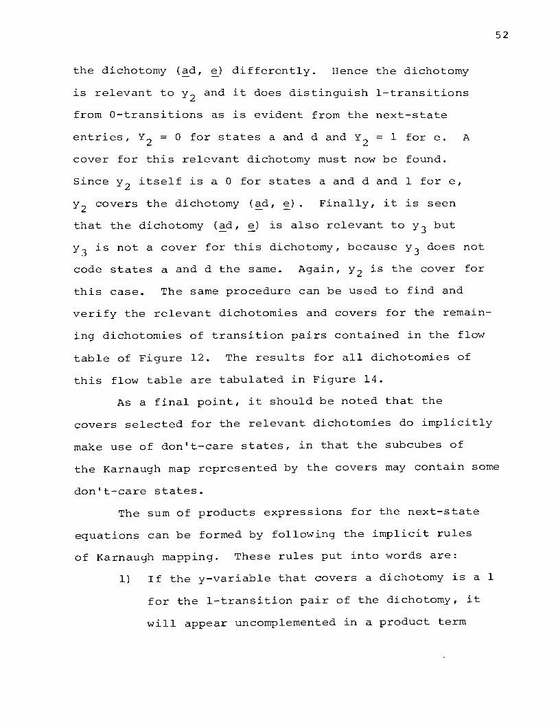
the dichotomy (ad, e) differently. Hence the dichotomy
is relevant to y 2 and it does distinguish 1-transitions
from a-transitions as lS evident from the next-state
entries, Y2 = 0 for states a and d and Y2
= 1 for e. A
cover for this relevant dichotomy must now be found.
Since y 2 itself is a 0 for states a and d and l for e,
y 2 covers the dichotomy (ad, ~). Finally, it is seen
that the dichotomy (ad, e) is also relevant to y3
but
y 3 is not a cover for this dichotomy, because y 3 does not
code states a and d the same. Again, y 2 is the cover for
this case. The same procedure can be used to find and
verify the relevant dichotomies and covers for the remain
ing dichotomies of transition pairs contained in the flow
table of Figure 12. The results for all dichotomies of
this flow table are tabulated in Figure 14.
As a final point, it should be noted that the
covers selected for the relevant dichotomies do implicitly
make use of don't-care states, in that the subcubes of
52
the Karnaugh map represented by the covers may contain some
don't-care states.
The sum of products expressions for the next-state
equations can be formed by following the implicit rules
of Karnaugh mapping. These rules put into words are:
l) If the y-variable that covers a dichotomy is a l
for the 1-transition pair of the dichotomy, it
will appear uncomplemented in a product term

Figure 11.
yl y2 y3 yl y2 y3
0 0 0 a 0 0 0
0 0 1 - d 0 0 0
0 1 1 e 0 1 1
0 1 0
1 1 0 b 1 0 0
1 1 1
1 0 1
1 0 0 c 1 0 0
Columnar Karnaugh Map Showing Next-State Entries Under Input I 1 of the Flow Table
in Figure 12
of the next-state expression. Conversely, if
it is a 0 for the 1-transition pair, it will
appear complemented in the product term.
2) If only one relevant dichotomy appears under
a particular input, or if more than one relevant
dichotomy appears but are covered by the same
y-variable, then a simple product term of the
form v.I will occur in the next-state equation "'-1 m
where ~i is the respective cover for the
dichotomies.
y. ) • l
(Note: ~i implies either yi or
3) If more than one relevant dichotomy appears
under a particular input, and each has a
53

54
different 1-transition pair then a product term
of the form (~i + ~j + ••• + ~n)Im will occur in
the next-state equation, where the state variables
in the term represent the respective covers for
the relevant dichotomies.
4) If the same 1-transition pair appears ln more
than one relevant dichotomy under a particular
input, then a product term of the form ~·~· l J
v I will occur in the next-state equation. Ln m
Conversely, if no dichotomies under a particular
input are relevant toy., then no product term l
for this input will occur in the equation for Y .. l
As an example of Tan's theory, the flow table which
was used in the previous methods will again be considered
here and is repeated in Figure 12.
Il I2 I3
a 0 b 0 b c ® ® c Q b a
d a 0 e
e 0 d 0 Figure 12. Flow Table
The first step would be to list all the destination
sets under each input.

DI DI DI 1 __ 2 3
a d a b c a c
b c d e b -e d e
From the destination sets the dichotomies of transition
pairs that can be formed are:
Il I2 I3
(a d, b c) (a b, d e) (a c, b)
(a d, e) (b c, d e) (~ c, d e)
(b c, e) (b 1 d e)
For the selection of the initial state variable, let y 1 induce the partition {(ad e) ,(b c)} such that states in
block (a d e) are coded with a 0 and states in block (b c)
55
are coded with a 1. A searching procedure is now initiated,
as shown in Figure 13, to find those dichotomies which are
relevant to y 1 .
It is observed in Figure 13 that two relevant dicho-
tomies are not covered. To cover these dichotomies the
state variables y 2 and y 3 , which induce the partitions
{(a c d), (be)} and {(abc) ,(de)} respectively, are
chosen. Therefore, yl = fl(Im' 01) where 01 = {yl' y2,
The table in Figure 13 is extended to include y2 and y3
in Figure 14. Notice that all dichotomies of the flow
y3}.
table are now covered and each state has a unique coding.
This means that the Tracey conditions are satisfied and

56
Partial Assignment Input Dichotomies yl States
0 a (ad, be) X
1 b Il (ad, e) -
1 c (be, e) X
0 d I2 ( ab ,de) I
0 e (be, de) X
(~c, b) I
I3 (ac, d~) -
(b 1 de) X
Legend
means not relevant
I means relevant to y. but not covered by y. l l
X means relevant to y. and covered by y. l l
Figure 13. Determination of Relevant Dichotomies
the USTT assgnment will also consist of the set {y1, y 2
, y3
}.
The equations for Y1 , Y2 , and Y3 can be written directly
from Figure 14 using the rules previously stated.
These equations are:
yl = ylil + y3I2 + Y1Y2I3
y2 = yly2Il + y3I2 + (y 2 + y3)I3
In some cases where two different variables cover the same
dichotomy either variable may be used in the product term.

57
Partial Assignment Input Dichotomies y1
y2
y3
yl y2 y3 States (ad, be) X - -
0 0 0 a Il (ad, e) - X I
1 1 0 b (be, e) X I X - -1 0 0 c
I2 (ab, de) I I X
0 0 1 d (be, de) X I X -
0 1 1 e (ac, b) I X --I3 (ac, de) - I X
(b' de) X - X
Figure 14. Complete Cover of Relevant Dichotomies
This is equivalent to having more than one choice in which
the 1-entries of a Karnaugh map can be circled.
It should now be pointed out that in the above
example the selection of the state variables was predeter-
mined. The state variables were chosen so that the
resulting assignment would be the same as the one used in
the conventional approach and in the Maki, Tracey and Smith
method. This was done to show that the same next-state
equations could be obtained with Tan's method as with these
other approaches.
This concludes the review of the fundamental theory
of Tan's iterative approach. A specific iterative procedure
developed by Tan [8] will now be discussed. This procedure
results in a Liu type assignment and so is only concerned

58
with destination sets and not with transition pairs. Hence,
the theory given above will be somewhat extended to a
destination set point of view.
2. Tan's Specific Iterative Procedure
In Tan's specific iterative procedure [8], the
derivation of the next-state equations is very similar
to the method used by Burton and Noaks. One difference
in the methods is that Tan does not start with a complete
initial assignment by assigning all destination sets a
unique y-variable. Instead, an initial partial-state
assignment is made by discreetly assigning only a few
y-variables to those destination sets which help minimize
the number of additional variables still needed for a
satisfactory USTT assignment.
Some guidelines for selecting this initial partial
state assignment are listed in the following priority:
1) Select those y-variables that will partition
the destination sets of more than one input
column in the same manner. Each additional
input column partitioned will result in a
savings of one y-variable in the final assign-
ment. One way in which these y-variables may
be found is by assigning a y-variable to a
destination set which appears in more than one
input column, because y-variables assigned to
the same destination sets will induce identical

partitions. This rule is essentially the same
as the Simplification Test II of Burton and
Noaks, which said that y-variables assigned to
equal destination sets are redundant and only
one y-variable is needed for all such sets.
2) Select those y-variables which take on the
binary value 0 for all the stable states in a
particular input column. These y-variables can
be determined by finding those induced parti-
tions in which all of the stable states of an
input column will appear in the 0 coded block
of the partition. If y. = 0 for all stable 1
states in an input column then no product term
for this input column will appear in the equa-
tion for Y .. 1
3) Select those y-variables such that in their
respective next-state equations, most of the
product terms also appear in some other equa-
tions. Hence, the cost of these equations will
likely be small.
The third selection criterion is the least definite of the
three and would probably only be used when criteria one
and two failed to yield a sufficient number of state
variables for an initial partial-state assignment. In
many cases this criterion will yield more variables than
what is actually needed for a. satisfactory partial-state
assignment. Therefore, the set of variables obtained from
59

this selection technique should be examined and just those
variables that are needed for a partial-state assignment
should be selected. An example of a partial-state
assignment would be an assignment which only satisfies
two columns of a four-column flow table.
The flow table shown in Figure 15 will now be
considered.
Il I2 I3
1 0 2 0 2 0 0 3
3 4 0 G) 4 0 5 1
5 2 G) 3
Figure 15. Flow Table
The destination sets for this table are:
1 1 2 1 4
2 5 3 2 3 5
3 4 4 5
In examining these destination sets, it is seen that no
y-variable can be selected which will induce identical
partitions on the destination sets of more than one input
column. Hence, criterion one of the selection technique
given above cannot be satisfied. However, criterion two
60

is satisfied by three state variables, in which the first
two, y 1 and y 2 , induce partitions on the destination
sets under input r 2 and the third, y 3 , induces a partition
on the destination sets under r3
.
their respective partitions are:
yl -r { ( 1 2 3) , ( 4 5) }
y2 -r { ( 1 2 4 5),{3)}
y3 -r { ( 2 3 5) , ( 1 4) }
Following the convention that the
These variables with
states in the first
block of the partition are coded with a 0 binary value
with respect to y. and in the second block a 1 binary l
value, notice that for each partition y. = 0 for all stable l
states of at least one input column, thus satisfying the
condition of criterion two. Also, these three state vari-
61
ables do form a partial-state assignment since they separate
the destination sets under input columns r 2 and r3
.
Once the initial partial-state assignment has been
determined the next-state equations for these variables
are then derived. To expedite the derivation of these
equations, essentially the same theory that was used in
Burton and Noaks' method is used in Tan's method. As
previously noted in Tan's method, each y-variable takes on
the value 1 for all states in the second block (1-block) of
its respective partition, while in Burton and Noaks' method
each variable takes on a value 1 for the states in its
associated destination set. (The associated destination
set is actually a 1-block of its corresponding induced

62
y-partition.) Even though in Tan's method a 1-block of a
y-partition may contain more than one destination set, the
derivation of the next-state equations is performed in
the same fashion, i.e., with the 1-blocks of the respective
partitions being treated in the same manner as the assoc-
iated destination sets in Burton and Noaks' method.
In Burton and Noaks' method, the equations for Y. l
consisted of product terms representing covers for those
destination sets having their stable states contained in
the associated y. destination set. l
Since each destination
set was initially associated with a unique y-variable, all
product terms could be immediately written in the equation.
However, this is not the case in Tan's method, since a
partial assignment does not separate all destination sets
in the flow table. Therefore, there may exist destination
sets having stable states which are contained in the 1-blocks
of the initial y-variable partitions (some 1-destination
sets) , but have not yet been separated by at least one
y-variable partition from the other destination sets
(0-destination sets), in their corresponding input column.
(Note: Insuring the separation of the 1-destination sets
from the a-destination sets is the same as covering the
relevant dichotomies of destination sets or transition
pairs as discussed in Tan's basic theory.) It should now
be clear that if some of the covers for the 1-destination
sets with respect to y. are not initially known, then some l
of the product terms in the equation for Y. cannot be l

63
immediately written. To determine those destination sets
which still lack covers and to provide assistance in the
selection of additional y-variables, a symbolic repre-
sentation of the next-state equations can be given by:
Y. + [a b ••• q] = ••• +I [de 1 n r] + •••
[ S] * +I f g ••• n ( 2 )
where y. = 1 for states [a b ·•• q]; states [de ••• r] l
are those contained in 1-destination sets with respect to
Yi under some input In, and are covered by at least one of
* they-variables of the initial set; [f g ••• s] are those
states contained in 1-destination sets under input I , but n
are not covered by any y-variable that has already been
chosen. Equations of this form will be referred to as
state transition equations. The state transition equations
for the initial assignment found above will be:
yl + [4 5] = I 1 [3 4] * + I2
[4 5]
y2 + [3] = I 2 [3] + I 3 [2 3 5]
* y3 + [1 4] = I 1 [1, 3 4] + I 3 [1 4]
Examining the above equations it is seen that the terms
* 4~J* I 1 [3 4] and I 1 [1, 3 are not covered by any one of
the variables of the initial assignment. The next step
is to assign new y-variables to those destination sets
that are contained in the starred product terms of the
state transition equations. In the example here, assign-
* and y 5 to I 1 [1, 3 4] will yield the
following partitions:

and
y4 + {(1 2 5) ,(3 4)}
y5
+ {(2 5),(1 3 4)}
Y4 + [3 4] = I 1 [3 4] + I 2 [3] + I 3 [2 3 5]
Y5 + [1 3 4] = I 1 [i, 3 4] + I 2 [3] + I 3
64
Since no more starred products were introduced in the state
transition equations for Y4 and Y5 , it would appear that
our assignment is complete. To be sure, the assignment
should be checked to see if the Liu conditions of separat-
ing all destination sets in an input column and distin-
guishing each state uniquely are satisfied. In this
example these conditions are satisfied and therefore the
set {y1 , y 2 , y 3 , y 4 , y 5 } forms a satisfactory USTT Liu
type assignment [7].
Converting the state-transition equations into
next-state equations can be done in a relatively easy and
straightforward manner. The destination sets contained
in the product terms of the state-transition equations will
be replaced by the y-variables (either y. or y.) of the l l
assignment, whose partitions have a block equal to these
destination sets. Following this rule, the next-state
equations can be written as:
yl = Ily4 + I2yl
y2 = I2y2 + I3y3
y3 = Ily5 + I3Y3
-------

y4 = Ily4 + I2y2 + I3Y3
YS = Ily5 + I2y2 + I3
Although the final assignment obtained may not be
a minimal assignment, the resulting next-state equations
are minimal and consist of only simple product terms.
Tan [8] also showed that some of the simple product
terms can be replaced by compound product terms if the
overall effect was to reduce the total number of gate
inputs required to realize the next-state equations. For
example, the term r 1y 5 in Y3 could be replaced by r1
(y2
+y3
)
since the sum of the 1-blocks of the y 2 and y 3 partitions
equals (1 3 4), the 1-block of the y 5 partition. However,
it can be shown that this replacement would not result in
a lower number of total gate inputs and therefore would
not be made (even though the replacement would eliminate
the need for y 5 in the assignment).
Reduced cost in terms of the number of gate inputs
required to logically realize the next-state equations is
a point that Tan [8] pursued very meticulously and
rigorously, by integrating a cost analysis with his
derivation of the next-state equations. With today's
technology in circuit packaging, especially in the areas
of integrated circuitry and module construction, it is
debatable whether the detailed cost study is worth increas
ing the complexity of his method.
65

66
This completes the description of Tan's specific
procedure. A summary of the steps of this method is:
1) Using the criteria of the selection technique,
select a set of state variables for the initial
partial-state assignment.
2) Derive the state-transition equations for the
variables in the initial assignment.
3) From the equations derived in step 2, generate
new variables for the assignment.
4) After a sufficient number of state variables
have been generated for a valid USTT Liu type
assignment, form the next-state equations for
these variables.
As an assistance in comparing this method with the
other methods discussed, a final example will be given for
the same flow table used in the previous methods.
Given a machine represented by the following flow
table:
11 12 13
a G b 0 Internal b c ® ® States c G b a
d a @ e
e 0 d 0

The destination sets for this flow table are:
DI 1
DI 2
DI 3
a d a b c a c -b c d e b -
e d e -By criterion one of the initial assignment selection
technique:
y 1 -+ {(abc) ,(de)}
By criterion 2:
y2
-+ {(a b c d), (e)}
y3
-+ {(a c de) ,(b)}
Since variables y 1 and y 3 will separate the destina
tion sets under inputs r 2 and r 3 , let the initial partial
state assignment consist of (y1 , y 3 ).
Next, the state-transition equations will be
67
constructed for the variables in the partial-state assignment.
* Y1 + [d e] = r 1 [e] + r 2 [d e] + r 3 [d e]
Y3 -+ [b] = r 2 [a b c] + r 3 [b]
* Now select a y-variable to cover the term r 1 [e] . Note
that this term will be covered by the partition
{(abc d), (e)} which is equal to the y 2 partition. There
fore, add y 2 to the assignment and derive its state
transition equation.

Since no more starred products have occurred, check to see
if the conditions for a valid Liu type assignment are
satisfied. In checking these conditions, it is found that
destination sets {a d} and {b c} under r 1 have not yet
been separated. Therefore assign:
y 4
+ {(a d e) , (b c)}
and
Y4
+ [b c] = r 1 [b c] + r 2 [a b c] + r 3[b]
Again, no further starred products have been generated and
the conditions for a valid USTT assignment are now satis-
68
fied. Therefore, the assignment consists of {y1 , y 2 , y 3 , y 4 }
and the corresponding next-state equations generated from
the state-transition equations are:
yl = Y2 1 1 + Y11 2 + Y1 1 3
y2 = Y2 1 1 + Y1 1 3
y3 = Y1 1 2 + Y3 1 3
y4 = Y4 1 1 + Y1 1 2 + y3I3
Although the results will vary for each flow table,
the above example points out some interesting highlights
of Tan's method. The resulting assignment has three less
variables than the assignment obtained using Burton and
Noaks ' method. Since both methods use the destination set
approach, the difference in their results is primarily
attributed to the use of complemented variables in Tan's
method while none are permitted in Burton and Noaks'
method. Also note that even though the number of y-variables

• I • • 1n Tan s ass1gnment 1s one greater than the number of
variables in the minimal assignment used in the conven-
tional approach, Tan's next-state equations require less
gate inputs to implement than do the equations of the
conventional approach.
Depending on the specifications of the design, Tan's
specific procedure may or may not be desirable. However,
it is conceivable that his basic theory could be used to
develop other specific iterative procedures or it could
be used on conjunction with other USTT assignment methods,
which may better meet the specifications of the design.
For example, Tan, Menon and Friedman [9,2] jointly
developed a method for generating a USTT assignment and
next-state equations by parallel and serial decompositions
of asynchronous sequential circuits. The method used for
generating the next-state equations is the same as that
discussed in Tan's basic theory. Therefore, only a brief
description of the decomposition method will be given
here, since the main goal of this paper is to present the
different known methods of generating next-state equations
and not necessarily that of finding the state assignment
itself.
Definition: Two partitions TI and n' on the set of
states of a sequential machine M are a partition pair
denoted by P(n, n') if for all states in the same block
69

of TI, their next-states to which the machine goes, when
any input Im is applied, are in the same block of rr'.
Definition: A partition TI on the states of a
sequential machine M is called a preserved partition if
for all states in the same block of rr, their next-states
to which the machine goes, when any input I is applied, m
are also in a common block of rr.
For a machine having the set of internal states
{a,b, c,d}, thepartitions,rr(O) ={(a), (b), (c), (d)}
and TI(l) = {(a,b,c,d)} always form preserved partitions
and are referred to as the trivial cases. Also from the
above definitions it should be apparent that a preserved
partition will form a partition pair with itself, i.e.,
P(TI, 'IT).
Each component machine of a decomposition is defined
by a partition pair P(TI, JT'), where the blocks of JT 1
correspond to the states of the submachine and the blocks
of 'IT correspond to the internal information required to
calculate the next-state of the submachine. In order to
obtain a decomposition resulting in a USTT assignment for
the component machines and therefore for the composite
machine, it is necessary that at least one non-trivial
preserved partition exists for the given flow table. This
preserved partition will form a partition pair with itself
which will define the first component machine of a serial
70

decomposition. The model of a serial decomposition is
shown in Figure l6(a) below.
I m
I m
Figure 16.
(a)
.. M l
- M2
(b)
(a) Serial Decomposition Decomposition
I J
.. : _:::
z Outpu~-Logic
Output z Logic
{b) Parallel
The product of the partitions induced by the y-variables
71
of the assignment for submachine M1 will equal the preserved
partition. Since M1 feeds M2 , the preserved partition of
M1 is an input partition to M2 • Therefore, the partition
pair that defines M2 will be a combination of the preserved
partition of M1 and the y-variable partitions that are
needed to cover the dichotomies of transition pairs of the
given flow table that were not covered by the assignment
These y-variables will form the state assignment

72
If two or more non-trivial preserved partitions exist
for the given flow table such that their product equals
TI(O), then these partitions will define submachines of a
parallel decomposition as shown in Figure 16(b). The out-
put logic recognizes the overall internal state of the
composite machine as a function of the internal states of
submachines M1 and M2
.
For flow tables that do not have any preserved
partitions, methods have been developed for decompositions
leading to multicode STT assignments and multiple transi
tion time assignments, but these methods will not be
discussed here [9].
The procedure terminates when all component machines
have a valid assignment which implies that the product
of ally-variable partitions equals TI(O). It has been
shown that the assignments and next-state equations of the
component machines will combine to yield a satisfactory
non-critical race assignment and next-state equations for
the composite or given machine [9,2].
To help clarify the above description, an example
will be given for the following flow table:

Il I2 I3 I4
1 0 0 4 2
2 0 3 0 0 3 0 G) 4
4 0 G) 5
5 0 1 0 Two preserved partitions for this flow table are:
'TTl = { (13)' (245)}
7T'"l = {(1),(2),(34),(5)} .:..
and
n 1 · n 2 = {(1),(2),(3),(4),(5)} = n(O)
Therefore, the preserved partitions n 1 and n 2 will form
partition pairs P(n1 ,n1 ) and P(n 2 ,n 2 ) which will define
component machines M1 and M2 of a parallel decomposition.
The flow tables representing the subrnachines M1 and
M2 are:
Subrnachine M1
Blocks Internal of n 1 States Il I2 I3 I4
( 13) a 0 0 b b
( 24 5) b G) a G G
73

74
Subrnachine M2
Blocks Internal of TI 2 States Il I2 I3 I4
( 1) A 0 0 c B
(2) B ® c ® ® ( 34) c @ @) @) D
( 5) D @ A @
The next step is to derive a USTT assignment and
corresponding next-state equations for each of the corn-
ponent flow tables. The most general approach which could
be used to accomplish this task is to derive the state
assignment for each component flow table using a known
state assignment procedure (e.g., the Tracey method [6]),
and then use Tan's basic theory to derive the corresponding
next-state equations. However 1 in this case, Tan's
specific iterative procedure was used to derive the follow-
ing state assignment and next-state equations simultan-
eously for each component flow table.
For subrnachine M1 :
State Assignment Next-State Equations
Internal yl States
0 a ( 13)
1 b ( 245)

75
And for subrnachine M2 :
State Assignment Next-State Equations
y2 y y4 Internal
3 States
0 1 1
1 1 0
0 0 0
A -
B -
c -
( 1)
( 2)
(34)
y2 = y2Il + y2I3 + y3I4
y3 = y3Il + y4I2 + y2I3 + Y3I4
y4 = y4Il + y4I2 + Y3I3
0 0 1 D - ( 5)
Now the assignment and corresponding next-state
equations for the composite machine is obtained by corn-
bining the results of the component machines. Therefore,
the composite state assignment and corresponding next-
state equations are:
Composite State Assignment Next-State Equations
Internal yl y2 y3 y4 States
0 0 1 1 1 yl = ylil + I3 + I4
1 1 1 0 2 y2 = y2Il + y2I3 + Y3 1 4
0 0 0 0 3 y3 = Y3 1 1 + Y4 1 2 + Y2 1 3 + Y3 1 4
1 0 0 0 4 y4 = Y4 1 1 + Y4 1 2 + Y3 1 3
1 0 0 1 5
This concludes the review of the presently known
methods for generating next-state equations. The remainder
of this paper will deal with a new method which was developed
from a study of the foregoing methods.

76
IV. NEW METHOD OF GENERATING NEXT-STATE EQUATIONS
Burton and Noaks' procedure and Tan's specific
procedure both have been directed toward the generation
of the next-state equations in parallel with the selection
of a USTT assignment. These methods may be desirable for
some designs since the Burton and Noaks method yields
next-state equations with no complemented variables, while
Tan's method may yield equations that require a low number
of gate inputs. However, in order to obtain the next-state
equations using these methods, their particular type of
assignments (Liu type) must also be used for the design.
Since methods have already been developed which
provide different types of USTT assignments for a flow
table (e.g., the Tracey method for a minimal variable
assignment) , a simple method for generating minimal next
state equations that could be used for any USTT assign
ment would be extremely valuable, especially for large
flow tables.
It has been shown that the Maki, Tracey and Smith
method and the basic theory of Tan can be used to obtain
next-state equations for any USTT assignment, but as flow
tables become larger the amount of work required to use
these methods becomes excessive and tedious. For example,
in Maki, Tracey and Smith's method the Boolean expressions
representing the specified states must be complemented to

obtain the expressions for the unspecified states. These
expressions in turn are combined with the expressions of
the 1-destination set subspaces to obtain minimal next-
state equations. It is obvious that much work and time
(computer time, too, if programmed) is required to perform
these manipulations and the necessary simplification to
obtain minimal equations. Also, when using Tan's basic
theory, all dichotomies of transition pairs must be
listed and then an exhaustive search for those state
variables that minimally cover the relevant dichotomies
must be carried out. Only after this is completed can
the heuristic rules be used to construct the next-state
equations. So again it is apparent that for large flow
tables an extreme amount of work and time is required,
since there would be many, many dichotomies of transition
pairs to examine. Therefore, the main intent here is to
develop a simple and straightforward method which will
require less work to generate minimal next-state equations
for any given USTT assignment and will easily lend itself
to computer application.
The heart of the following method of generating
next-state equations emanates from the role that the
Karnaugh map plays in separating the 1-destination sets
from the a-destination sets. It was believed that if
the operations performed with a Karnaugh map could some
how be carried out implicitly in a simple and straight
forward manner, a powerful means for generating the
77

78
next-state equations would result. To show why such a
method would be a powerful tool, the flow table used in
the previous methods, repeated in Figure 17, will again
be considered here.
yl y2 y3 Il I2 I3
0 0 0 a 0 b 0 1 1 0 b c G) G) 1 0 0 c 0 b a
0 0 1 d a 0 e
0 1 1 e 0 d 0 Figure 17. Flow Table
The destination sets for this table are:
a d a b c a c
b c d e b
e d e
The Karnaugh map of the USTT assignment for this
table is shown in Figure 16.
yly2 00 01 11 10
0 a - b c
1 d e - -
Figure 18. Karnaugh Map

79
Now suppose that the next-state equation Y1
is to
be calculated. In order to successfully derive the minimal
equation for Y1 , minimal y-variable covers must be found
for each input column which separate the 1-destination sets
subspaces from the a-destination set subspaces. The
1-destination sets with respect to y 1 under each input
are:
b c a b c b
From the Karnaugh map it is seen that the state variable
y 1 separates the subspace of the 1-destination set (b c)
from the remaining a-destination set subspaces under I1
.
Therefore, the minimal cover for this separation can be
written as the simple product term y 1 I 1 . It should be
noted that the don't-care states are again being used
implicitly here, since they are in the subcube covered by
y 1 . Similarly, the minimal cover for the subspace of
(a b c) under I 2 is the simple product term y 3I 2 and for
the subspace of (b) under I 3 the minimal cover can be
Therefore, from a knowledge of
the 1- and a-destination sets and with the use of the
Karnaugh map, the equation for Y1 can be written by
inspection as:
The above equation is a minimal next-state equation
and agrees with the results obtained in the conventional

sa
approach, the Maki, Smith and Tracey method and the approach
used in the basic theory of Tan. The reason the above
equation is in minimal form is because the y-variable
covers were selected in such a manner to separate the
largest possible subcubes containing the 1-destination
sets (thus inherently making use of don't-care states) from
the subcubes of the a-destination sets.
It should now be apparent that, by using the Karnaugh
map in the above manner, the derivation of the next-state
equations can be accomplished in a simpler and faster
manner than in the previous methods.
When working with the Karnaugh map in the above
example, the operations were performed either by hand or
were done mentally. The goal of the following method will
be to describe these same operations in a definite language
that would permit computer application for large flow
tables.
Definition: A two block partition a .. is called l,J
the a-partition with respect toY. and input I. if the - l J
left block contains all the internal states for which
Y. =a under input I. and the right block contains all l J
the internal states for which Y. = 1 under input I .. l J
This definition implies that the left-block of an
a-partition will contain the states in a-destination
sets while the right block will contain the states in
1-destination sets, all with respect to some y. and I .. l J

For an example, the flow table in Figure 17 will again be
considered. The 0- and 1-destination sets with respect to
y 1 and under input I. are: J
0-destination Sets 1-destination Sets
a d b c
e
Therefore, a 1 , 1 can be written as:
a 1 , 1 ={(ad e),(b c)}
Similarly,
a 1 2 ={(de) ,(abc)} '
a 1 , 3 ={(a c d e),(b)}
Comparing with the conventional approach, it is
seen that the above a-partitions indicate which states
will have either 0- or 1-entries in the Karnaugh maps
that were derived from the transition table for Y1
(see
Figure 5, page 11). Therefore, the a-partitions provide
part of the information attainable from the Karnaugh
81
maps. Of course, the remaining portion of information that
is obtained with the Karnaugh map is the selection of a
minimal y-variable cover that separates the a-destination
sets from the 1-destination sets.
Definition: A set A of· states is said to cover a
set B of states if B c A (read as set B is contained in
or equal to set A) .

It should be kept in mind that since the word ''cover"
takes on several different meanings, any particular mean-
ing must be derived from the context in which it is being
used.
It is known from the conditions for a valid USTT
assignment that all of the states in 1-destination sets
are separated from those in 0-destination sets. These
separations are provided by the state variables of the
assignment as was shown in the first example by the
Karnaugh map in Figure 18. Therefore, it follows that
the covers of the a-partitions can be obtained from the
partitions induced by the y-variables of the assignment.
Definition: A two block partition, T., is called l
a T-partition with respect to yi' if the left block
contains all of the internal states for which y. = 0 and l
the right block contains all the internal states for
which y. = 1. l
The concept of this definition has already been used
in the previous methods of Tan and Burton and Noaks. The
definition implies that the states in the left block of
a T· partition are covered by they-variable expression l
y. while the states in the right block are covered by l
the expression yi. The T-partitions induced by the state
variables in the assignment of the example are:
82

83
yl yl
-r 1 ={(ad e) 1 (b c)}
y2 y2
T2 = {(a c d) 1 (b e) }
y3 y3
T = 3 {(a b c) 1 (d e)}
The y-variable covers for all blocks have been explicitly
shown.
The next step is to find which blocks of the
-r-partitions separate the blocks of the a-partitions.
This separation can be accomplished by selecting those
blocks of the -r-partitions that together cover the right
block (Y = 1 block) of the a-partition and do not contain
any states from the left block of the a-partition.
(Those blocks satisfying the second condition are referred
to as being disjoint from the left block of the a-partition.)
For example, to separate the blocks of a 1 , 1 =
{(ad e) 1 (b c)} a cover for the block (b c) is needed.
Examining the -r-partitions, it is observed that the right
block of -r 1 would be the most minimal cover because it
equals (b c) itself. Now, since the block (b c) is
covered by y1
in the -r 1 partition, it can be concluded
that y1
will separate the blocks of a 1 , 1 and Y111 can be
written as:

where Yi,j represents the next-state variable yi under
input I .. J
84
Here again the use of unspecified states in obtaining
the y-variable cover is inherent in the T-partitions. For
example, from the Karnaugh map of Figure 18 (page 78) , it
is seen that T1 actually implies the partition
yl yl
T 1 = { ( ade-) , (be--) } ,
where y 1 covers the subcube spanned by specified states
b and c and two unspecified states. It is this inherent
characteristic of T-partitions that enables a minimal
y-variable next-state expression to be obtained.
Similarly for a 1 , 2 ={(de) ,(abc)}, block (abc)
is covered by the left block of T3
•
Yl,2 = y3I2
Therefore,
Now for a 1 3 ={(a c de) ,(b)}, there is no single block , of the T-partitions that covers block (b) and does not
contain any of the states in block (a d c e) . In other
words, under input I 3 , there is no single y-variable that
separates the 1-destination sets from the a-destination
sets with respect to y 1 . Therefore, it is necessary to
examine the product partitions of the form T. · T .. l J
partitions will be the g.l.b. partition of T. l
and T .. J
In our example, the product partitions of the form
T. • T . are: l J
These

yly2 yly2 yly2 yly2 'l · T 2 ={(a d),(e),( c ,(b)}
yly3 yly3 yly3 yly3 'l · T 3 = {(a),(d e),(b c),( 0 )}
Again the appropriate y-variable cover is associated with
each block. As an example, the first block of 'l • T 2 is
obtained by intersecting the y 1 block of 'l with the y 2
block of T 2 , i.e.:
yl y2 (a d e) () (a c d) = etc.
85
Now the blocks of the T. l
• T. partitions are examined J
to find a cover for block (b) of a 1 , 3 . It is seen that
block (b) can be covered by either block y 1 y 2 of 'l · T 2
or block y2
y3
of T 2 • ,3
. This is the same choice of
covers that existed in the preceding example with the
Karnaugh map. Choosing y 1 y 2 as the cover, then:
The expressions for Yl,l' Y1 , 2 , and Yl,J can now be combined
to give:
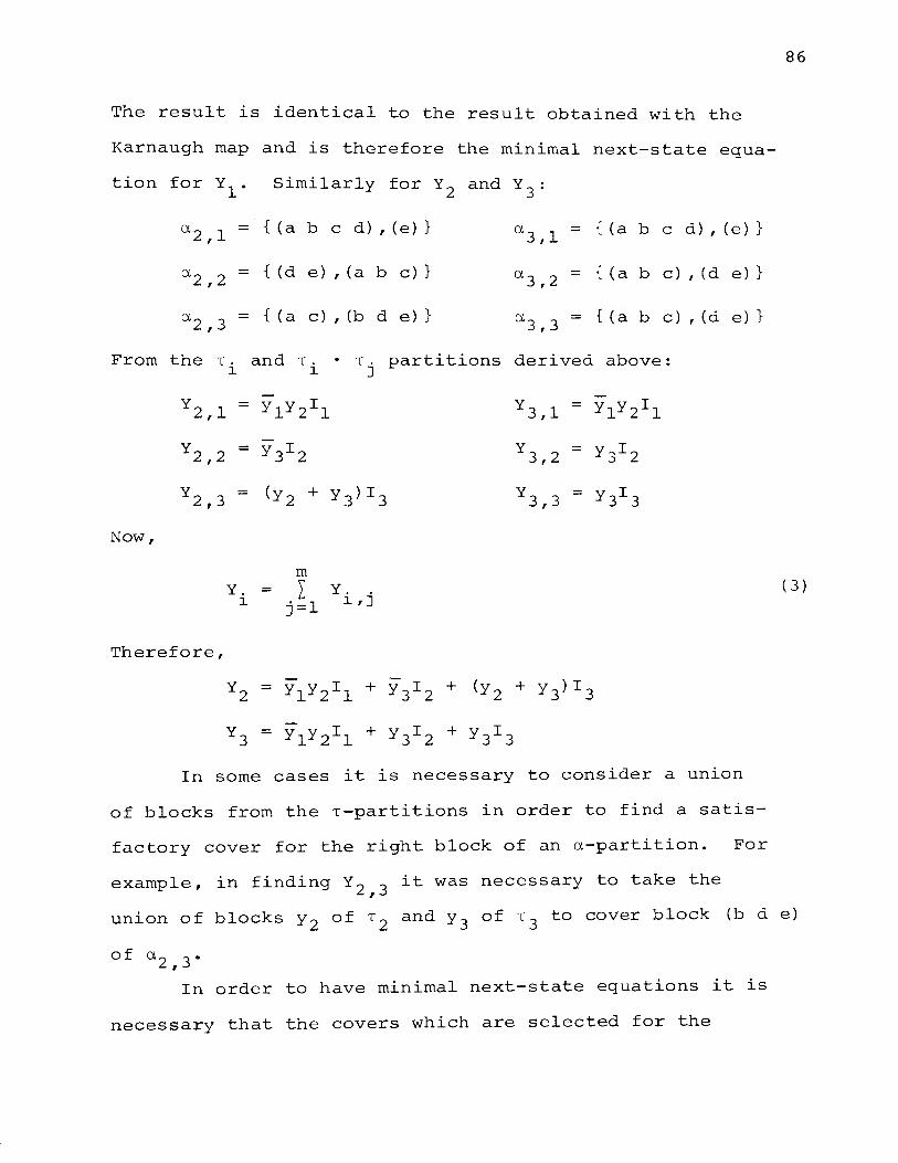
The result is identical to the result obtained with the
Karnaugh map and is therefore the minimal next-state equa-
tion for Y1
. Similarly for Y2
and Y3
:
a2,1 = { (a b c d),(e)} a3,1 = { (a b c d),(e)}
a2,2 = { (d e) , (a b c) } a3,2 = { (a b c) ' (d e) }
a2,3 = { (a c) , (b d e) } a3,3 = {(a b c) , (d e) }
From the T. and T. l l
• Tj partitions derived above:
Now,
Y2,1 =
Y2,2
Y2,3
=
=
Y. l
Y1Y2I1
y3I2
(y 2 +
m I
j=l
y3)I3
Y .. l,J
y 3 '1 =
Y3,2 =
Y3,3 =
Therefore,
y2 = yly2Il + y3I2 + (y2 + y3)I3
y3 = yly2Il + y3I2 + y3I3
Y1Y2I1
y3I2
y3I3
In some cases it is necessary to consider a union
of blocks from the T-partitions in order to find a satis-
factory cover for the right block of an a-partition. For
example, in finding Y2 , 3 it was necessary to take the
86
( 3)
union of blocks y 2 of T2 and y 3 of T3 to cover block (b d e)
of a 2 , 3 •
In order to have minimal next-state equations it is
necessary that the covers which are selected for the

blocks of the a-partitions are the minimal covers for
those blocks. For instance, a union of two blocks from
some T-partitions would not be a minimal cover and hence
would not be used, if a cover exists which consists of
only one block from some other T-partition. The minimal
cover corresponds to the largest possible circling of "1"
and "don't-care" entries in the Karnaugh map. This can
be seen by comparing the minimal covers found for Y1 in
the above example with the circlings in the Karnaugh maps
that were used in the conventional approach (Figure 5).
87
Rules for selecting the minimal covers in a systematic
and orderly fashion can be established. One strategy
which could be formalized into such a set of rules is:
1) Check the blocks of the a-partition. If its
left block or its right block equals the empty
set, then the product term corresponding to
this partition in the equation for Y .. will l,J
just be I. or 0 respectively. J
2) If neither block of the a-partition equals the
empty set, then select all blocks from the
T-partitions, that are disjoint from the left
block of the a-partition. Check these blocks
to see if any single block will cover the right
block of the a-partition. If one of these
blocks does cover the right block of the
a-partition, then the equation for Y .. can be l,J
written as a simple product term. If no single

block exists, check the union of the previously
selected disjoint blocks taken two at a time.
If still no cover exists, check the union of
these blocks taken three at a time, etc., until
a cover is found.
3) If none of the blocks of the T-partitions are
disjoint from the left block of the a-partition,
or if only a partial cover can be obtained with
step 2, then form the T. · T. partitions and l J
follow the rules of step 2 until a complete
cover is found.
4) If still no complete cover has been obtained,
repeat the process with the product partitions
T. • T. • Tk' etc., until a complete cover is l J
found.
Before proceeding with a final example, a summary of
the steps of this method is:
1) List all of the destination sets for each input
column of the flow table.
2) From the destination sets under each input,
form the a-partitions with respect to yi by
putting the a-destination sets in the left
block and the 1-destination sets in the right
block.
3) Form the T-partitions that are induced by the
state variables of the given assignment.
88

4) From the blocks of the T-partitions, find a
cover for the right block of the a-partition
by following the strategy for the selection of
a minimum cover.
5) The next-state equations are then derived from
they-variables representing the selected covers.
The final example will be for a larger flow table
in order to show the capability and proficiency of this
method.
Suppose that an asynchronous sequential circuit is
described by the following flow table having the USTT
state assignment as shown.
0
0
0
1
0
1
1
0
1
1
0
1
0
1
1
0
0
1
0
1
0
0
0
1
0 0
0 1
1 0
0 0
1 0
0 1
0 1
1 1
1 0
1 1
1 1
1 0
a
b
c
d
e
f
g
h
i
j
k
1
d 0 e b
f G) h G) 1 ~ e b
0 0 g b
i a 0 b
0 g 0 b
d ® 0 b
f G) b
(;) j g b
k CD g b
(E) a h b
0 c 0 b
89

90
The destination sets for this flow table are:
Dr 1
Dr 2
Dr 3
DI 4
a d g a e k a c e a b c d e f g h i j k 1 - -b f h b f
e i c 1 - d ~ l j
j k d b h k
c 1 f .9. 1
i j
The a.-partitions with respect to each Y. and I. are: l J
a,lll = {(jk) 1 (abcdefghil)} 0,211 = { (adegijk) 1 (bcfhl)}
a.l,2 = { (abcekl) 1 (dfgij)} 0,212 = { (adefgijk) 1 (bel)}
0,113 = { (abcehk), (dfgijl)} 0,213 = { (acdegij) , (bfhkl) }
0,114 = {(abcdefghijkl), (~)} a.2,4 = {(~) 1 (abcdefghijkl)}
0,311 = {(abdfgh), (ceijk1)} 0,4 1 1 = { (acdegil) 1 (bfhjk)}
0,312 = { ( ab de f gk) 1 ( c i j 1 ) } a,4 2 = { (acdekl) 1 (bfgij)} 1
0,313 = { (dfgij) 1 (abcehkl)} (t 4 1 3 = { ( acel) 1 (bdfghi jk) }
0,314 = {(abcdefghijkl) ,(~)} 0,414 = {(~) 1 (abcdefghijkl)}
The T-partitions induced by the state variables of
the assignment are:
yl yl T
1 = { (abcehk) 1 (dfgij 1) }

y2 y2 T2 = {(adegijk) ,(bcfhl)}
y3 y3 T3 = {(abdfg) ,(cehijkl)}
y4 y4 T4 = {(acdeil), (bfghjk)}
From the T-partitions, the T. · T. partitions will l J
now be formed to have them available if needed.
yly2 yly2 yly2 yly2 Tl . T2 = {(a e k), (b c h) 1 (d g i j),(f 1)}
yly3 yly3 yly3 yly3
Tl . TJ = {(a b) , ( c e h k) 1 (d f g) 1 (i j 1) }
yly4 yly4 yly4 yly4
Tl . T4 = { (a c e) , (b h k) 1 (d i l),(fgj)}
Y2Y3 y2y3 y2y3 y2y3
T2 . TJ = { (a d g) , ( e i j k) , (b f) , (c h 1)}
y2y4 y2y4 y2y4 y2y4
T2 . T4 = {(a d e i) , ( g J k) 1 (C 1) 1 (b f h) }
Y3Y4 Y3Y4 Y3Y4 Y3Y4 T
3 • T 4 ={(a d),(b f g),(c e i l),(h j k)}
The next step is to find a minimum cover for the
right block of the a-partitions. For an example, take the
right block of a 1 , 1 , (abcdefghi). Therefore, find a
minimal cover for (abcdefghi) from the block of the
T-partitions such that the cover is disjoint from (jk),
the left block of a 1 , 1 .
91

y2 y3 y4 Cover of ( abcdefghi) = (bcfhl) u ( abdfg) u (acdeil)
Therefore,
yl 1 = (y 2 + y3 + y4)Il I
Similarly:
Yl,2 = (yly2 + yly3)I2 Y2,1 = Y2 1 1
yl 3 = Yl 1 3 Y2,2 = (yly2 + Y2Y3)I2 I
yl 4 = 0 Y2,3 = (yly2 + yly4)I3 I
Y2,4 = I4
y3 1 = (y2y3 + Y2Y4)Il Y4,1 = (y2y 4 + y3y4)Il I
Y3,2 = (yl y 3 + Y2Y4)I2 y4 2 = (y3y4 + yly2y3)I2 I
Y3,3 = (yl + y2y3)I3 Y4,3 = (y 4 + yly2)I3
Y3,4 = 0 Y4,4 = I4
Note that in order to find Y4 , 2 it was necessary to
form Tl • T2 • T3 . That is:
yly2y3 yly2y3 yly2y3 yly2y3 Tl • T
2 • T
3 = {( a ),( b ),( d g),( f ),
Now the cover of:
yly2y3 yly2y3 yly2y3 yly2y3 (ek),( h ),(ij),( 1 )}
y3y4 yly2y3 (bfgij) = (bfg) u (ij)
92

93
The expressions for the covers associated with the
a-partitions have now been found. The minimal next-state
equations can be derived by simply combining these
expressions.
Y. = Y. 1 + y. 2 + Y. 3 + y. 4 l l, l, l., l,
Therefore,
yl = (y 2 + y3 + y4)I1. + (y 1 y2 + yly3) 1 2 + yli3
y2 = Y2 1 1 + (yly2 + y2y3)I2 + (yly2 + yly4)I3 + I4
y3 = (y2y3 + Y2Y4)Il + (yly3 + y2y4)I2 + (yl + Y2Y3)I3
y4 = (y 2y 4 + Y3Y4)Il + (y 3y 4 + yly2y3)I2 + (y4 + yly2)I3 + I4
From the above example the value of this method with
respect to large flow tables can be readily seen. There-
fore, the method could play a key role in future synthesis
applications. It should be made clear that this method is
a general method for only generating next-state equations
and does not generate the state assignment too.

V. CONCLUSION
Now that each of the methods for generating the next
state equations for normal-mode asynchronous sequential
circuits has been described, a meaningful discussion and
comparison of their strengths and weaknesses can be made.
First of all, one major difference that should be
remembered is that the state assignment must be derived
independently and prior to the use of the Maki, Tracey and
Smith method and the new method developed in this paper.
On the other hand, Burton and Noaks' method and Tan's
method are used to derive both the state assignment and
next-state equations in a parallel fashion. (Note: The
basic theory of Tan's method can also be used for just
deriving the next-state equations for a given state
assignment.) As a result of this difference the method
of Burton and Noaks and the specific procedure of Tan's
method are somewhat limited as general methods for gener-
ating next-state equations. In order to obtain the next-
state equations using these methods, their particular
type of state assignments must also be used. Therefore,
these methods could not be utilized in cases where a
design specified the use of a state assignment that
differed from their particular assignments. However,
the Maki, Tracey and Smith method, Tan•s basic theory and
94

the new method developed in this paper are general methods
which will work for any type of uni-code single transition
time (USTT) assignment that is given.
Another interesting comparison is the use of the
unspecified states of a flow table as a tool for obtain-
95
ing minimal next-state equations. The Maki, Tracey and
Smith method is the only method that handles the unspecified
states in an explicit fashion. The other methods
implicitly use the unspecified states. This difference
results because, in the Maki, Tracey and Smith method, the
y-variable expression that covers a transition pair
subspace is selected in such a manner that it covers the
smallest subcube of a Karnaugh map that contains that
transition pair. Then other y-variable expressions need
to be derived to cover the subcubes of the unspecified
states. In the other methods, however, the y-variable
expressions which cover particular transition pairs (or
destination sets) are selected in a manner such that they
cover the largest possible subcube of a Karnaugh map that
contains the transition pairs (or destination sets) along
with any available unspecified states. Therefore, the
unspecified states are inherent in these covers.
It is the explicit handling of the unspecified
states that leads to the following disadvantages of the
Maki, Tracey and Smith method:

1) The amount of time and work required to find the
expressions for the unspecified states by taking
the logical complement.
2) The amount of time and work required to simplify
the expressions to a set of minimal equations.
A recommendation for partially alleviating the above
disadvantages without changing the entire strategy can be
given. Part of the time and work required above is a
result of using transition pairs as the basis of their
method. For assignments derived from a transition pair
basis, it is necessary that their method also uses the
transition pair basis in the derivation of the next-state
equations. However, if the given state assignment is
known to be one based upon destination sets, then some
work and time would be saved if the method could be
readily converted to use destination sets as its basis
rather than transition pairs. A savings would result
because the unsimplified Boolean expressions produced by
destination sets would have fewer terms than the equiva-
lent expressions produced by transition pairs. Thus, the
manipulations required in the above disadvantage would
become less unwieldy.
The best method with respect to the mechanics
required in the actual construction of the next-state
equations is Burton and Noaks' method. The shortcuts
used in their derivation result from the way the initial
state assignment is made, i.e., the association of a
96

unique y-variable with each destination set. This state
assignment also leads to the unique property of having no
complemented variables in the next-state equations, which
may be a desirable feature for some designs.
It is recalled that Tan also used a strategy similar
to Burton and Noaks' for construction of the next-state
equations in his specific iterative procedure. The
1-blocks of the y-variable partitions in Tan's procedure
are treated in the same manner as the associated y-variable
destination sets in Burton and Noaks' method. However,
Tan's resulting next-state equations are not complement
free because both the 0-blocks and 1-blocks of the
y-variable partitions are used as possible covers in the
next-state equation.
One characteristic of Burton and Noaks' method which
may be a disadvantage is that a larger assignment and,
therefore, more state variables, have to be contended with
in the design. This evaluation can be verified by noting
that for the same flow table used in the example of each
method, the resulting Burton and Noaks' assignment exceeded
the assignments of all other methods by at least three
state variables. Of course, the effectiveness of this
method will vary from circuit to circuit. And there may
be cases where a minimal variable assignment could be
obtained with this method, but generally the method will
realize a larger assignment. This can be considered as
the price paid for complement free next-state equations.
97

Another disadvantage of Burton and Noaks' method is
the informal procedure of simplifying the initial assign
ment using a dependency diagram. A more formal procedure
capable of being programmed on a computer would certainly
be welcomed.
From his basic theory, Tan developed a specific
iterative procedure which results in a Liu type assign
ment. Although his assignment may not be a minimum
variable assignment, it often results in minimal next
state equations requiring less gate inputs to implement.
This is due to the discreet manner in which the state
variables are selected for the assignment.
It has also been shown that Tan's basic theory can
be used strictly as a next-state equation generation
method for any given USTT assignment. However, as in the
case of the Maki, Tracey and Smith method, it too requires
a considerable amount of work and time for larger flow
tables. This is because, in using Tan's basic theory,
all dichotomies of transition pairs must be listed and
then an exhaustive search for those state variables that
minimally cover the relevant dichotomies must be carried
out. Even after the covers for the relevant dichotomies
have been determined, the derivation of the next-state
equations requires another rather complicated step. In
this step, the relevant dichotomies have to be further
examined to determine whether the uncomplement or
98

complement form of the y-variable covers should be used
and whether the product terms will be simple or compound
in the final next-state expression. As flow tables
become larger, a greater number of dichotomies have to
be examined and the amount of work and time required
becomes excessive.
99
The new method developed in this paper seems to
provide a better means of coping with larger flow tables.
In this method all destination sets (and therefore transi
tion pairs) are grouped into one two-block partition per
input column, i.e., the a-partition. Therefore, no matter
how large the flow table is, in the derivation of a next
state equation it is only necessary to cover one a-partition
per input column; whereas, in Tan's basic theory, many
dichotomies per input column have to be examined and
covered. It is this reason that enables the new method to
handle larger flow tables more efficiently than the other
methods. Since many practical circuits are very large, it
is conceivable that this method could become a valuable
tool in the future in the synthesis of asynchronous sequen
tial circuits. Also, another attribute of this method is
its applicability to be programmed for computer use.
Since the new method is a systematic repetitive
procedure, it, too, has the disadvantage of becoming some
what lengthy for larger flow tables when a large number of
T-partitions and products of T-partitions have to be
considered.

100
This completes a comparison of the foregoing methods.
In deciding which method should be used, the strengths
and weaknesses of each method mentioned above would have
to be weighed for the particular problem at hand.

VI. BIBLIOGRAPHY
1. E. J. McCluskey, Introduction to the Theory of Switching Circuits. New York:--McGraw-Hill,-rnc., 1965.
2. S. H. Unger, Asynchronous Sequential Switching Circuits. New York: John W1ley and Sons., Inc., 1969.
3. G. K. Maki, J. H. Tracey, and R. J. Smith, "Generation of design equations in asynchronous sequential circuits," IEEE Trans. on Computers, vol. C-18, pp. 467-472, May 1969.
4. R. J. Smith, J. H. Tracey, W. L. Schoeffel, and G. K. Maki, "Automation in the design of asynchronous sequential circuits," 1968 Spring Joint Computer Conf., AFIPS Proc., Vol. 32, pp. 55-60, 1968.
101
5. D. P. Burton and D. R. Noaks, "Complement free STT state assignments for asynchronous sequential machines," Proceedings of the 2nd National Symposium on Logic Design, University of Reading, Sponsored by British Computer Society, March 1969.
6. J. H. Tracey, "Internal state assignments for asynchronous sequential machines," IEEE Trans. on Electronic Computers, vol. EC-15, pp. 551-560, August 1966.
7. C. N. Liu, "A state variable assignment method for asynchronous sequential switching circuits," J. ACM, vol. 10, pp. 209-216, April 1963.
8. c. J. Tan, "Synthesis of asynchronous sequential switching circuits," Dr. Eng. Sc. Dissertation, Columbia University, June 1969.
9. C. J. Tan, P. R. Menon, and A. D. Friedman, "Structural simplification and decomposition of asynchronous sequential circuits," IEEE Trans. on Computers, vol. C-18, pp. 830-838, September 1969.
VII. VITA
Gregory Martin Bednar was born on June 26, 1944, in
St. Louis, ~1issouri. He was graduated valedictorian of
his class from Cuba High School, Cuba, Missouri. He
received a Bachelor of Science degree in Electrical Engi
neering from the University of Missouri - Rolla in August,
1966. He was actively employed by IBM at Rochester,
Minnesota, from August 1966 to September 1967, after
which he began two years active duty as an officer in
the United States Ar,my. One year was spent in Vietnam
where he was awarded the bronze star and the bronze star
with oak leaf cluster. Presently, he is enrolled in the
Graduate School of the University of Missouri - Rolla in
Electrical Engineering.
The author is a member of IEEE, Eta Kappa Nu,
Tau Beta Pi, and Phi Kappa Phi.
102