nfft 3.0 - tutorial - tu chemnitzpotts/nfft/guide/nfft3.pdf · this tutorial surveys the fast...

NFFT 3.0 - Tutorial

Jens Keiner∗ Stefan Kunis† Daniel Potts‡

http://www.tu-chemnitz.de/∼potts/nfft

∗[email protected],University of Lubeck, Institute of Mathematics, 23560 Lubeck†[email protected], Chemnitz University of Technology, Department of Mathematics, 09107

Chemnitz, Germany‡[email protected], Chemnitz University of Technology, Department of Mathematics, 09107

Chemnitz, Germany

1

Contents

1 Introduction 3

2 Notation, the NDFT, and the NFFT 52.1 NDFT - nonequispaced discrete Fourier transform . . . . . . . . . . . . . . . 52.2 NFFT - nonequispaced fast Fourier transform . . . . . . . . . . . . . . . . . . 62.3 Available window functions and evaluation techniques . . . . . . . . . . . . . 102.4 Further NFFT approaches . . . . . . . . . . . . . . . . . . . . . . . . . . . . . 13

3 Generalisations and inversion 143.1 NNFFT - nonequispaced in time and frequency fast Fourier transform . . . . 143.2 NFCT/NFST - nonequispaced fast (co)sine transform . . . . . . . . . . . . . 143.3 NSFFT - nonequispaced sparse fast Fourier transform . . . . . . . . . . . . . 153.4 FPT - fast polynomial transform . . . . . . . . . . . . . . . . . . . . . . . . . 153.5 NFSFT - nonequispaced fast spherical Fourier transform . . . . . . . . . . . . 163.6 Solver - inverse transforms . . . . . . . . . . . . . . . . . . . . . . . . . . . . . 19

4 Library 234.1 Installation . . . . . . . . . . . . . . . . . . . . . . . . . . . . . . . . . . . . . 234.2 Procedure for computing an NFFT . . . . . . . . . . . . . . . . . . . . . . . . 244.3 Generalisations and nomenclature . . . . . . . . . . . . . . . . . . . . . . . . . 254.4 Inversion and solver module . . . . . . . . . . . . . . . . . . . . . . . . . . . . 28

5 Examples 315.1 Computing your first transform . . . . . . . . . . . . . . . . . . . . . . . . . . 315.2 Computation time vs. problem size . . . . . . . . . . . . . . . . . . . . . . . . 315.3 Accuracy vs. window function and cut-off parameter m . . . . . . . . . . . . 325.4 Computing an inverse transform . . . . . . . . . . . . . . . . . . . . . . . . . 33

6 Applications 346.1 Summation of smooth and singular kernels . . . . . . . . . . . . . . . . . . . . 346.2 Fast Gauss transform . . . . . . . . . . . . . . . . . . . . . . . . . . . . . . . . 346.3 Summation of zonal functions on the sphere . . . . . . . . . . . . . . . . . . . 346.4 Iterative reconstruction in magnetic resonance imaging . . . . . . . . . . . . . 356.5 Computation of the polar FFT . . . . . . . . . . . . . . . . . . . . . . . . . . 356.6 Radon transform, computer tomography, and ridgelet transform . . . . . . . . 36

References 36

2

1 Introduction

This tutorial surveys the fast Fourier transform at nonequispaced nodes (NFFT), its gener-alisations, its inversion, and the related C library NFFT 3.0. The goal of this manuscriptis twofold – to shed some light on the mathematical background, as well as to provide anoverview over the C library to allow the user to use it effectively. Following this, this docu-ment splits into two parts:

In Sections 2, 3 and 3.6, we introduce the NFFT which, as a starting point, leads to severalconcepts for further generalisation and inversion. We focus on a mathematical descriptionof the related algorithms. However, we complement the necessarily incomplete quick glanceat the ideas by references to related mathematical literature. In Section 2, we introducethe problem of computing the discrete Fourier transform at nonequispaced nodes (NDFT),along with the notation used and related works in the literature. The algorithms (NFFT)are developed in pseudo code. Furthermore, we turn for recent generalisations, includingin particular NFFTs on the sphere and iterative schemes for inversion of the nonequispacedFFTs, in Section 3 and 3.6, respectively.

Having laid the theoretical foundations, Section 4 provides an overview over the NFFT3.0 C library and the general principles for using the available algorithms in your own code.Rather than describing the library interface in every detail, we restrict to simple recipes inorder to familiarise with the very general concepts sufficient for most everyday tasks. For theexperienced user, we provide full interface documentation (see doc/html/index.html in thepackage directory) which gives detailed information on more advanced options and parametersettings for each routine. Figure 1.1 gives an overview over the directory structure of theNFFT 3.0 package. Finally, Section 5 gives some simple examples for using the library andsome more advanced applications are given in Section 6 along with numerical results.

3

doc[internal doxygen docs]

include[interface]

util[utility functions]

kernel

fpt[fast polynomial transform]

mri[transform in magnetic resonance imaging]

nfct[nonequispaced fast cosine transform]

nfft[nonequispaced fast Fourier transform]

nfsft[nonequispaced fast spherical Fourier transform]

nfst[nonequispaced fast sine transform]

nnfft[nonequispaced in space and frequency FFT]

nsfft[nonequispaced sparse fast Fourier transform]

solver[inverse transforms]

examples[for each kernel]

applications

fastgauss[fast Gauss transform]

fastsum[summation schemes]

fastsumS2[summation on the sphere]

mri[reconstruction in mri]

nfft flags[time and memory requirements]

polarFFT[fast polar Fourier transform]

radon[radon transform]

stability[stability inverse nfft]

Figure 1.1: Directory structure of the NFFT 3.0 package

4

2 Notation, the NDFT, and the NFFT

This section summarises the mathematical theory and ideas behind the NFFT. Let the torus

Td :={

x = (xt)t=0,...,d−1 ∈ Rd : −12≤ xt <

12, t = 0, . . . , d− 1

}of dimension d ∈ N be given. It will serve as domain from which the nonequispaced nodes xare taken. Thus, the sampling set is given by X := {xj ∈ Td : j = 0, . . . ,M − 1}.

Possible frequencies k ∈ Zd are collected in the multi-index set

IN :={

k = (kt)t=0,...,d−1 ∈ Zd : −Nt

2≤ kt <

Nt

2, t = 0, . . . , d− 1

},

where N = (Nt)t=0,...,d−1 is the EVEN multibandlimit, i.e., Nt ∈ 2N. To keep notation sim-ple, the multi-index k addresses elements of vectors and matrices as well, i.e., the plain indexk :=

∑d−1t=0 (kt + Nt

2 )∏d−1

t′=t+1Nt′ is not used here. The inner product between the frequencyindex k and the time/spatial node x is defined in the usual way by kx := k0x0 + k1x1 +. . .+ kd−1xd−1. Furthermore, two vectors may be combined by the component-wise product

σ �N := (σ0N0, σ1N1, . . . , σd−1Nd−1, )> with its inverse N−1 :=

(1

N0, 1

N1, . . . , 1

Nd−1

)>.

The space of all d-variate, one-periodic functions f : Td → C is restricted to the space ofd-variate trigonometric polynomials

TN := span(e−2πik· : k ∈ IN

)with degree Nt (t = 0, . . . , d − 1) in the t-th dimension. The dimension dimTN of the space

of d-variate trigonometric polynomials TN is given by dimTN = |IN | =d−1∏t=0

Nt.

2.1 NDFT - nonequispaced discrete Fourier transform

The first problem to be addressed can be regarded as a matrix vector multiplication. For afinite number of given Fourier coefficients fk ∈ C, k ∈ IN , we consider the evaluation of thetrigonometric polynomial

f (x) :=∑

k∈IN

fke−2πikx (2.1)

at given nonequispaced nodes xj ∈ Td. Thus, our concern is the evaluation of

fj = f (xj) :=∑

k∈IN

fke−2πikxj , (2.2)

j = 0, . . . ,M − 1. In matrix vector notation this reads

f = Af (2.3)

where

f := (fj)j=0,...,M−1 , A :=(e−2πikxj

)j=0,...,M−1; k∈IN

, f :=(fk

)k∈IN

.

5

The straightforward algorithm for computing this matrix vector product, which is calledNDFT, takes O(M |IN |) arithmetical operations.

A closely related matrix vector product is the adjoint NDFT

h = Aaf , hk =M−1∑j=0

fje2πikxj ,

where Aa = A> denotes the conjugate transpose of the nonequispaced Fourier matrix A.

Equispaced nodes

For d ∈ N, Nt = N ∈ 2N, t = 0, . . . , d − 1 and M = Nd equispaced nodes xj = 1N j, j ∈ IN

the computation of (2.3) is known as multivariate discrete Fourier transform (DFT). In thisspecial case, the input data fk are called discrete Fourier coefficients and the samples fj

can be computed by the well known fast Fourier transform (FFT) with only O(|IN | log |IN |)arithmetic operations. Furthermore, one has the inversion formula

AAa = AaA = |IN |I,

which does NOT hold true for the nonequispaced case in general.

2.2 NFFT - nonequispaced fast Fourier transform

For the sake of simplicity, we explain the ideas behind the NFFT for the one-dimensionalcase d = 1 and the algorithm NFFT. The generalisation of the FFT is an approximativealgorithm and has computational complexity O (N logN + log (1/ε)M), where ε denotes thedesired accuracy. The main idea is to use standard FFTs and a window function ϕ which iswell localised in the time/spatial domain R and in the frequency domain R. Several windowfunctions were proposed in [15, 7, 55, 25, 24].

The considered problem is the fast evaluation of

f (x) =∑k∈IN

fke−2πikx (2.4)

at arbitrary nodes xj ∈ T, j = 0, . . . ,M − 1.

The ansatz

One wants to approximate the trigonometric polynomial f in (2.4) by a linear combinationof shifted 1-periodic window functions ϕ as

s1 (x) :=∑l∈In

gl ϕ

(x− l

n

). (2.5)

With the help of an oversampling factor σ > 1, the FFT length is given by n := σN .

6

The window function

Starting with a reasonable window function ϕ : R → R, one assumes that its 1-periodicversion ϕ, i.e.

ϕ (x) :=∑r∈Z

ϕ (x+ r)

has an uniformly convergent Fourier series and is well localised in the time/spatial domain Tand in the frequency domain Z. The periodic window function ϕ may be represented by itsFourier series

ϕ (x) =∑k∈Z

ck (ϕ) e−2πikx

with the Fourier coefficients

ck (ϕ) :=∫T

ϕ (x) e2πikx dx =∫R

ϕ (x) e2πikx dx = ϕ (k) , k ∈ Z.

−0.5 0 0.510

−20

10−15

10−10

10−5

−0.5 0 0.510

−20

10−15

10−10

10−5

−32 −20 −12 0 11 19 3210

−20

10−15

10−10

10−5

100

Figure 2.1: From left to right: Gaussian window function ϕ, its 1-periodic version ϕ, andthe integral Fourier-transform ϕ (with pass, transition, and stop band) for N =24, σ = 4

3 , n = 32.

The first approximation - cut-off in frequency domain

Switching from the definition (2.5) to the frequency domain, one obtains

s1 (x) =∑k∈In

gk ck (ϕ) e−2πikx +∑

r∈Z\{0}

∑k∈In

gk ck+nr (ϕ) e−2πi(k+nr)x

with the discrete Fourier coefficients

gk :=∑l∈In

gl e2πi kln . (2.6)

Comparing (2.4) to (2.5) and assuming ck (ϕ) small for |k| ≥ n− N2 suggests to set

gk :=

{fk

ck(ϕ) for k ∈ IN ,0 for k ∈ In\IN .

(2.7)

7

Then the values gl can be obtained from (2.6) by

gl =1n

∑k∈IN

gk e−2πi kln (l ∈ In),

a FFT of size n.This approximation causes an aliasing error.

The second approximation - cut-off in time/spatial domain

If ϕ is well localised in time/space domain R it can be approximated by a function

ψ (x) = ϕ (x)χ[−mn

, mn

] (x)

with suppψ[−m

n ,mn

], m � n, m ∈ N. Again, one defines its one periodic version ψ with

compact support in T asψ (x) =

∑r∈Z

ψ (x+ r) .

With the help of the index set

In,m (xj) := {l ∈ In : nxj −m ≤ l ≤ nxj +m}

an approximation to s1 is defined by

s (xj) :=∑

l∈In,m(xj)

gl ψ

(xj −

l

n

). (2.8)

Note, that for fixed xj ∈ T, the above sum contains at most (2m+ 1) nonzero summands.This approximation causes a truncation error.

The case d > 1

Starting with the original problem of evaluating the multivariate trigonometric polynomial in(2.1) one has to do a few generalisations. The window function is given by

ϕ (x) := ϕ0 (x0)ϕ1 (x1) . . . ϕd−1 (xd−1)

where ϕt is an univariate window function. Thus, a simple consequence is

ck (ϕ) = ck0 (ϕ0) ck1 (ϕ1) . . . ckd−1(ϕd−1) .

The ansatz is generalised to

s1 (x) :=∑l∈In

gl ϕ(x− n−1 � l

),

where the FFT size is given by n := σ�N and the oversampling factors by σ = (σ0, . . . , σd−1)>.

Along the lines of (2.7) one defines

gk :=

{fk

ck(ϕ) for k ∈ IN ,0 for k ∈ In\IN .

8

The values gl can be obtained by a (multivariate) FFT of size n0 × n1 × . . .× nd−1 as

gl =1|In|

∑k∈IN

gk e−2πik(n−1�l), l ∈ In.

Using the compactly supported function ψ (x) = ϕ (x)χ[−mn

, mn

]d (x), one obtains

s (xj) :=∑

l∈In,m(xj)

gl ψ(xj − n−1 � l

),

where ψ again denotes the one periodic version of ψ and the multi-index set is given by

In,m (xj) := {l ∈ In : n� xj −m1 ≤ l ≤ n� xj +m1} .

The algorithm

In summary, the following Algorithm 1 is obtained for the fast computation of (2.3) withO (|In| log |In|+mM) arithmetic operations.

Input: d,M ∈ N, N ∈ 2Nd

Input: xj ∈ [−12 ,

12 ]d, j = 0, . . . ,M − 1, and fk ∈ C, k ∈ IN ,

1: For k ∈ IN compute

gk :=fk

|In| ck (ϕ).

2: For l ∈ In compute by d-variate FFT

gl :=∑

k∈IN

gk e−2πik(n−1�l).

3: For j = 0, . . . ,M − 1 compute

fj :=∑

l∈In,m(xj)

gl ψ(xj − n−1 � l

).

Output: approximate values fj , j = 0, . . . ,M − 1.Complexity: O(|N | log |N |+M).

Algorithm 1: NFFT

Algorithm 1 reads in matrix vector notation as

Af ≈ BFDf ,

where B denotes the real M × |In| sparse matrix

B :=(ψ

(xj − n−1 � l

))j=0,...,M−1; l∈In

,

9

where F is the Fourier matrix of size |In|× |In|, and where D is the real |In|× |IN | ’diagonal’matrix

D :=d−1⊗t=0

(Ot |diag (1/ ckt (ϕt))kt∈INt

|Ot

)T

with zero matrices Ot of size Nt × nt−Nt2 .

The corresponding computation of the adjoint matrix vector product reads as

Aaf ≈ D>F aB>f .

With the help of the transposed index set

I>n,m (l) := {j = 0, . . . ,M − 1 : l−m1 ≤ n� xj ≤ l +m1} ,

one obtains Algorithm 2 for the adjoint NFFT. Due to the characterisation of the nonzero

Input: d,M ∈ N, N ∈ 2Nd

Input: xj ∈ [−12 ,

12 ]d, j = 0, . . . ,M − 1, and fj ∈ C, j = 0, . . . ,M − 1,

1: For l ∈ In computegl :=

∑j∈I>n,m(l)

fj ψ(xj − n−1 � l

).

2: For k ∈ IN compute by d-variate (backward) FFT

gk :=∑l∈In

gl e+2πik(n−1�l).

3: For k ∈ IN compute

hk :=gk

|In| ck(ϕ).

Output: approximate values hk, k ∈ IN .Complexity: O(|N | log |N |+M).

Algorithm 2: NFFTa

elements of the matrix B, i.e.,

M−1⋃j=0

j × In,m (xj) =⋃

l∈In

I>n,m (l)× l.

the multiplication with the sparse matrix B> is implemented in a ’transposed’ way in thelibrary, summation as outer loop and only using the multi-index sets In,m (xj).

2.3 Available window functions and evaluation techniques

Again, only the case d = 1 is presented. To keep the aliasing error and the truncation errorsmall, several functions ϕ with good localisation in time and frequency domain were proposed,

10

e.g. the (dilated) Gaussian [15, 55, 14]

ϕ (x) = (πb)−1/2 e−(nx)2

b

(b :=

2σ2σ − 1

m

π

), (2.9)

ϕ (k) =1n

e−b(πkn )2

,

(dilated) cardinal central B–splines [7, 55]

ϕ (x) = M2m (nx) , (2.10)

ϕ (k) =1n

sinc2m (kπ/n) ,

where M2m denotes the centred cardinal B–Spline of order 2m,(dilated) Sinc functions [45]

ϕ (x) =N (2σ − 1)

2msinc2m

((πNx (2σ − 1))

2m

), (2.11)

ϕ (k) = M2m

(2mk

(2σ − 1)N

)and (dilated) Kaiser–Bessel functions [30, 25]

ϕ (x) =1π

sinh(b√m2 − n2x2

)√m2 − n2x2

for |x| ≤ mn

(b := π

(2− 1

σ

)),

sin(b√n2x2 −m2

)√n2x2 −m2

otherwise,

(2.12)

ϕ (k) =1n

I0

(m

√b2 − (2πk/n)2

)for k = −n

(1− 1

2σ

), . . . , n

(1− 1

2σ

),

0 otherwise,

where I0 denotes the modified zero–order Bessel function. For these functions ϕ it has beenproven that

|f (xj)− s (xj) | ≤ C (σ,m) ‖f‖1

where

C (σ,m) :=

4 e−mπ(1−1/(2σ−1)) for (2.9) ,

4(

12σ−1

)2mfor (2.10) ,

1m−1

(2

σ2m +(

σ2σ−1

)2m)

for (2.11) ,

4π (√m+m) 4

√1− 1

σ e−2πm√

1−1/σ for (2.12) .

Thus, for fixed σ > 1, the approximation error introduced by the NFFT decays exponentiallywith the number m of summands in (2.8). Using the tensor product approach the aboveerror estimates can be generalised for the multivariate setting [18]. On the other hand, thecomplexity of the NFFT increases with m.

In the following, we suggest different methods for the compressed storage and application ofthe matrix B which are all available within our NFFT library by choosing particular flags in asimple way during the initialisation phase. These methods do not yield a different asymptoticperformance but rather yield a lower constant in the amount of computation.

11

Fully precomputed window function

One possibility is to precompute all values ϕ(xj−n−1�l) for j = 0, . . . ,M−1 and l ∈ In,m(xj)explicitly. Thus, one has to store the large amount of (2m+ 1)dM real numbers but uses noextra floating point operations during the matrix vector multiplication beside the necessary(2m+ 1)dM flops. Furthermore, we store for this method explicitly the row and column foreach nonzero entry of the matrix B. This method, included by the flag PRE FULL PSI, is thefastest procedure but can only be used if enough main memory is available.

Tensor product based precomputation

Using the fact that the window functions are built as tensor products one can store ϕt((xj)t−ltnt

) for j = 0, . . . ,M − 1, t = 0, . . . , d − 1, and lt ∈ Int,m((xj)t) where (xj)t denotes the t-th component of the j-th node. This method uses a medium amount of memory to stored(2m + 1)M real numbers in total. However, one has to carry out for each node at most2(2m+1)d extra multiplications to compute from the factors the multivariate window functionϕ(xj − n−1 � l) for l ∈ In,m(xj). Note, that this technique is available for every windowfunction discussed here and can be used by means of the flag PRE PSI which is also the defaultmethod within our software library.

Linear interpolation from a lookup table

For a large number of nodes M , the amount of memory can by further reduced by the use oflookup table techniques. For a recent example within the framework of gridding see [6]. Wesuggest to precompute from the even window function the equidistant samples ϕt( rm

Knt) for

t = 0, . . . , d − 1 and r = 0, . . . ,K, K ∈ N and then compute for the actual node xj duringthe NFFT the values ϕt((xj)t − lt

nt) for t = 0, . . . , d− 1 and lt ∈ Int,m((xj)t) by means of the

linear interpolation from its two neighbouring precomputed samples.This method needs only a storage of dK real numbers in total where K depends solely

on the target accuracy but neither on the number of nodes M nor on the multidegree N .Choosing K to be a multiple of m, we further reduce the computational costs during theinterpolation since the distance from (xj)t − lt

ntto the two neighbouring interpolation nodes

and hence the interpolation weights remain the same for all lt ∈ Int,m((xj)t). This methodrequires 2(2m+ 1)d extra multiplications per node and is used within the NFFT by the flagPRE LIN PSI. Error estimates for this approximation are given in [36].

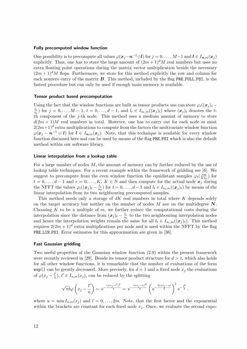
Fast Gaussian gridding

Two useful properties of the Gaussian window function (2.9) within the present frameworkwere recently reviewed in [29]. Beside its tensor product structure for d > 1, which also holdsfor all other window functions, it is remarkable that the number of evaluations of the formexp() can be greatly decreased. More precisely, for d = 1 and a fixed node xj the evaluationsof ϕ(xj − l′

n ), l′ ∈ In,m(xj), can be reduced by the splitting

√πbϕ

(xj −

l′

n

)= e−

(nxj−l′)2

b = e−(nxj−u)2

b

(e−

2(nxj−u)

b

)l

e−l2

b .

where u = min In,m(xj) and l = 0, . . . , 2m. Note, that the first factor and the exponentialwithin the brackets are constant for each fixed node xj . Once, we evaluate the second expo-

12

nential, its l-th power can be computed consecutively by multiplications only. Furthermore,the last exponential is independent of xj and these 2m + 1 values are computed only oncewithin the NFFT and their amount is negligible. Thus, it is sufficient to store or evaluate 2Mexponentials for d = 1. The case d > 1 uses 2dM storages or evaluations by using the generaltensor product structure. This method is employed by the flags FG PSI and PRE FG PSI forthe evaluation or storage of 2d exponentials per node, respectively.

No precomputation of the window function

The last considered method uses no precomputation at all, but rather evaluates the univariatewindow function (2m+ 1)dM times. Thus, the computational time depends on how fast wecan evaluate the particular window function. However, no additional storage is necessarywhich suits this approach whenever the problem size reaches the memory limits of the usedcomputer.

2.4 Further NFFT approaches

Several papers have described fast approximations for the NFFT. Common names for NFFTare non-uniform fast Fourier transform [24], generalised fast Fourier transform [15], unequally-spaced fast Fourier transform [7], fast approximate Fourier transforms for irregularly spaceddata [57], non-equispaced fast Fourier transform [26] or gridding [53, 30, 42].

In various papers, different window functions were considered, e.g. Gaussian pulse taperedwith a Hanning window in [14], Gaussian kernels combined with Sinc kernels in [42], andspecial optimised windows in [30, 14].

A simple but nevertheless fast scheme for the computation of (2.3) in the univariate cased = 1 is presented in [1]. This approach uses for each node xj ∈ [−1

2 ,12) a m-th order Taylor

expansion of the trigonometric polynomial in (2.1) about the nearest neighbouring point onthe oversampled equispaced lattice {n−1k− 1

2}k=0,...,n−1 where again n = σN, σ � 1. Besidesits simple structure and only O(N logN +M) arithmetic operations, this algorithm utilisesm FFTs of size n compared to only one in the NFFT approach, uses a medium amount ofextra memory, and is not suited for highly accurate computations, see [36]. Furthermore, itsextension to higher dimensions has not been considered so far.

Another approach for the univariate case d = 1 is considered in [16] and based on a Lagrangeinterpolation technique. After taking a N -point FFT of the vector f in (2.3) one uses anexact polynomial interpolation scheme to obtain the values of the trigonometric polynomialf at the nonequispaced nodes xj . Here, the time consuming part is the exact polynomialinterpolation scheme which can however be realised fast in an approximate way by meansof the fast multipole method. This approach is appealing since it allows also for the inversetransform. Nevertheless, numerical experiments in [16] showed that this approach is far moretime consuming than Algorithm 1 and the inversion can only be computed in a stable wayfor almost equispaced nodes [16].

Furthermore, special approaches based on scaling vectors [40], based on minimising theFrobenius norm of certain error matrices [41] or based on min-max interpolation [24] areproposed. While these approaches gain some accuracy for the Gaussian or B-Spline windows,no reasonable improvement is obtained for the Kaiser-Bessel window function.

For comparison of different approaches, we refer to [57, 41, 24, 36].

13

3 Generalisations and inversion

We consider generalisations of the NFFT for

3.1 NNFFT - nonequispaced in time and frequency fast Fourier transform

Now we are interested in the computation of

fj =N−1∑k=0

fke−2πi(vk�N))xj

for j = 0, . . . ,M − 1, vk,xj ∈ Td, and fk ∈ C, where N ∈ Nd denotes the ”nonharmonic”bandwidth. The corresponding fast algorithm is known as fast Fourier transform for noneq-uispaced data in space and frequency domain (NNFFT) [15, 18, 52] or as type 3 nonuniformFFT [38].

A straightforward evaluation of this sum with the standard NFFT is not possible, since thesamples in neither domain are equispaced. However, an so-called NNFFT was first suggestedin [15] and later studied in more depth in [18], which permits the fast calculation of the Fouriertransform of a vector of nonequispaced samples at a vector of nonequispaced positions. Itconstitutes a combination of the standard NFFT and its adjoint see also [52].

3.2 NFCT/NFST - nonequispaced fast (co)sine transform

Let nonequispaced nodes xj ∈ [0, 12 ]d and frequencies k in the index sets

ICN :=

{k = (kt)t=0,...,d−1 ∈ Zd : 0 ≤ kt < Nt, t = 0, . . . , d− 1

},

ISN :=

{k = (kt)t=0,...,d−1 ∈ Zd : 1 ≤ kt < Nt, t = 0, . . . , d− 1

}be given. For notational convenience let furthermore cos(k�x) := cos(k0x0)·. . .·cos(kd−1xd−1)and sin(k � x) := sin(k0x0) · . . . · sin(kd−1xd−1).

The nonequispaced discrete cosine and sine transforms are given by

f (xj) =∑

k∈ICN

fk cos(2π(k � xj)),

f (xj) =∑

k∈ISN

fk sin(2π(k � xj)),

for j = 0, . . . ,M − 1 and real coefficients fk ∈ R, respectively.The straight forward algorithm of this matrix vector product, which is called ndct and

ndst, takes O(M |ICN |) and O(M |IC

N |) arithmetical operations. For these real transforms theadjoint transforms coincide with the ordinary transposed matrix vector products. Our fastapproach is based on the NFFT and seems to be easier than the Chebyshev transform basedderivation in [44] and faster than the algorithms in [56] which still use FFTs. Instead of FFTswe use fast algorithms for the discrete cosine transform (DCT–I) and for the discrete sinetransform (DST–I). For details we refer to [22].

14

3.3 NSFFT - nonequispaced sparse fast Fourier transform

We consider the fast evaluation of trigonometric polynomials from so-called hyperbolic crosses.In multivariate approximation one has to deal with the so called ‘curse of dimensionality’,i.e., the number of degrees of freedom for representing an approximation of a function with aprescribed accuracy depends exponentially on the dimensionality of the considered problem.This obstacle can be circumvented to some extend by the interpolation on sparse grids and therelated approximation on hyperbolic cross points in the Fourier domain, see, e.g., [58, 54, 9].

Instead of approximating a Fourier series on the standard tensor product grid I(N,...,N)

with O(Nd) degrees of freedom, it can be approximated with only O(N logd−1N) degrees offreedom from the hyperbolic cross

HdN :=

⋃N∈Nd, |IN |=N

IN ,

where N = 2J+2, J ∈ N0 and we allow Nt = 1 in the t-th coordinate in the definition of IN .The approximation error in a suitable norm (dominated mixed smoothness) can be shown todeteriorate only by a factor of logd−1N , cf. [54].

Figure 3.1: Hyperbolic cross points for d = 2 and J = 0, . . . , 3.

The nonequispaced sparse discrete Fourier transform (NSDFT) is the evaluation of

f (xj) =∑

k∈HdN

fke−2πikxj

for given Fourier coefficients fk ∈ C and nodes xj ∈ Td. The number of used arithmeticaloperations is O(MN logd−1N). This is reduced by our fast schemes to O(N log2N +M) ford = 2 and O(N3/2 logN +M) for d = 3, see [20] for details.

3.4 FPT - fast polynomial transform

A discrete polynomial transform (DPT) is a generalisation of the DFT from the basis of com-plex exponentials eikx to an arbitrary systems of algebraic polynomials satisfying a three-termrecurrence relation. More precisely, let P0, P1, . . . : [−1, 1] → R be a sequence of polynomialsthat satisfies a three-term recurrence relation

Pk+1(x) = (αkx+ βk)Pk(x) + γkPk−1(x),

15

with αk 6= 0, k ≥ 0, P0(x) := 1, and P−1(x) := 0. Clearly, every Pk is a polynomial of exactdegree k and typical examples are the classical orthogonal Jacobi polynomials P (α,β)

k .Now, let f : [−1, 1] → R be a polynomial of degree N ∈ N given by the finite linear

combination

f(x) =N∑

k=0

akPk(x).

The discrete polynomial transform (DPT) and its fast version, the fast polynomial transform(FPT), are the transformation of the coefficients ak into coefficients bk from the orthogonal ex-pansion of f into the basis of Chebyshev polynomials of the first kind Tk(x) := cos(k arccosx),i.e.,

f(x) =N∑

k=0

bkTk(x).

A direct algorithm for computing this transformation needsO(N2) arithmetic operations. TheFPT algorithm implemented in the NFFT library follows the approach in [51] and is based onthe idea of using the three-term-recurrence relation repeatedly. Together with a method forfast polynomial multiplication in the Chebyshev basis and a cascade-like summation process,this yields a method for computing the polynomial transform with O(N log2N) arithmeticoperations. For more detailed information, we refer the reader to [12, 13, 51, 44, 32] and thereferences therein.

3.5 NFSFT - nonequispaced fast spherical Fourier transform

Fourier analysis on the sphere has, despite other fields, practical relevance in tomography,geophysics, seismology, meteorology and crystallography. In analogy to the complex expo-nentials eikx on the torus, the spherical harmonics form the orthogonal Fourier basis withrespect to the usual inner product on the sphere.

Spherical coordinates

Every point in R3 can be described in spherical coordinates by a vector (r, ϑ, ϕ)> with theradius r ≥ 0 and two angles ϑ ∈ [0, π], ϕ ∈ [0, 2π). We denote by S2 the two-dimensional unitsphere embedded into R3, i.e.

S2 :={x ∈ R3 : ‖x‖2 = 1

}and identify a point from S2 with the corresponding vector (ϑ, ϕ)>. The spherical coordinatesystem is illustrated in Figure 3.2.

Legendre polynomials and associated Legendre functions

The Legendre polynomials Pk : [−1, 1] → R, k ≥ 0, as classical orthogonal polynomials aregiven by their corresponding Rodrigues formula

Pk(x) :=1

2kk!dk

dxk

(x2 − 1

)k.

16

r

x2x1

x3

ϑ

ϕ

ξ

Figure 3.2: The spherical coordinate system in R3: Every point ξ on a sphere with radius rcentred at the origin can be described by angles ϑ ∈ [0, π], ϕ ∈ [0, 2π) and theradius r ∈ R+. For ϑ = 0 or ϑ = π the point ξ coincides with the North or theSouth pole, respectively.

The associated Legendre functions Pnk : [−1, 1] → R, k ≥ n ≥ 0 are defined by

Pnk (x) :=

((k − n)!(k + n)!

)1/2 (1− x2

)n/2 dn

dxnPk(x).

For n = 0, they coincide with the Legendre polynomials Pk = P 0k . The associated Legendre

functions Pnk obey the three-term recurrence relation

Pnk+1(x) =

2k + 1((k − n+ 1)(k + n+ 1))1/2

xPnk (x)− ((k − n)(k + n))1/2

((k − n+ 1)(k + n+ 1))1/2Pn

k−1(x)

for k ≥ n ≥ 0, Pnn−1(x) = 0, Pn

n (x) =√

(2n)!

2nn!

(1− x2

)n/2. For fixed n, the set {Pnk : k ≥ n}

forms a set of orthogonal functions, i.e.,

〈Pnk , P

nl 〉 =

∫ 1

−1Pn

k (x)Pnl (x)dx =

22k + 1

δk,l.

Again, we denote by Pnk =

√2k+1

2 Pnk the orthonormal associated Legendre functions. In the

following, we allow also for n < 0 and set Pnk := P−n

k in this case.

Spherical harmonics

The spherical harmonics Y nk : S2 → C, k ≥ |n|, n ∈ Z, are given by

Y nk (ϑ, ϕ) := Pn

k (cosϑ) einϕ.

17

They form an orthogonal basis for the space of square integrable functions on the sphere, i.e.,

〈Y nk , Y

ml 〉 =

∫ 2π

0

∫ π

0Y n

k (ϑ, ϕ)Y ml (ϑ, ϕ) sinϑ dϑ dϕ =

4π2k + 1

δk,lδn,m.

The orthonormal spherical harmonics are denoted by Y nk =

√2k+14π Y n

k .Hence, any square integrable function f : S2 → C has the expansion

f =∞∑

k=0

k∑n=−k

f(k, n)Y nk ,

with the spherical Fourier coefficients f(k, n) =⟨f, Y n

k

⟩. The function f is called bandlimited,

if f(k, n) = 0 for k > N and some N ∈ N. In analogy to the NFFT on the Torus T, we definethe sampling set

X :={(ϑj , ϕj) ∈ S2 : j = 0, . . . ,M − 1

}of nodes on the sphere S2 and the set of possible ”frequencies”

IN := {(k, n) : k = 0, 1, . . . , N ; n = −k, . . . , k} .

The nonequispaced discrete spherical Fourier transform (NDSFT) is defined as the evaluationof the finite spherical Fourier sum

fj = f (ϑj , ϕj) =∑

(k,n)∈IN

fnk Y

nk (ϑj , ϕj) =

N∑k=0

k∑n=−k

fnk Y

nk (ϑj , ϕj) (3.1)

for j = 0, . . . ,M − 1. In matrix vector notation, this reads f = Y f with

f := (fj)M−1j=0 ∈ CM , fj := f (ϑj , ϕj) ,

Y := (Y nk (ϑj , ϕj))j=0,...,M−1; (k,n)∈IN

∈ CM×(N+1)2 ,

f :=(fn

k

)(k,n)∈IN

∈ C(N+1)2 .

The corresponding adjoint nonequispaced discrete fast spherical Fourier transform (adjointNDSFT) is defined as the evaluation of

hnk =

M−1∑j=0

f (ϑj , ϕj)Y nk (ϑj , ϕj)

for all (k, n) ∈ IN . Again, in matrix vector notation, this reads h = Y a f .The coefficients hn

k are, in general, not identical to the Fourier coefficients f(k, n) of thefunction f . However, provided that for the sampling set X a quadrature rule with weightswj , j = 0, . . . ,M − 1, and sufficient degree of exactness is available, one might recover theFourier coefficients f(k, n) by evaluating

fnk =

∫ 2π

0

∫ π

0f(ϑ, ϕ)Y n

k (ϑ, ϕ) sinϑ dϑ dϕ =M−1∑j=0

wjf (ϑj , ϕj)Y nk (ϑj , ϕj)

18

Input: N ∈ N0, M ∈ N, spherical Fourier coefficients f = (fnk )(k,n)∈IN

∈ C(N+1)2 ,Input: a sampling set X = (ϑj , ϕj)

M−1j=0 ∈ ([0, π]× [0, 2π))M .

for n = −N, . . . , N doCompute the Chebyshev coefficients (bnk)N

k=0 of gn by a fast polynomial transform.Compute the coefficients (cnk)N

k=−N from the coefficients (bnk)Mk=0.

end forCompute the function values (f (ϑj , ϕj))

M−1j=0 by evaluating the Fourier sum using a fast

two-dimensional NFFT.

Output: The function values f = (f (ϑj , ϕj))M−1j=0 ∈ CM .

Complexity: O(N2 log2N +M

).

Algorithm 3: Nonequispaced fast spherical Fourier transform (NFSFT)

Input: N ∈ N0, M ∈ N, a sampling set X = (ϑj , ϕj)M−1j=0 ∈ ([0, π]× [0, 2π))M ,

Input: values f = (fj)M−1j=0 ∈ CM .

Compute the coefficients (cnk)Nk,n=−N from the values (fj)

N−1j=0 .

for n = −N, . . . , N do

Compute the coefficients(bnk

)N

k=0from the coefficients (cnk)N

k=−N .

Compute the coefficients (ank)N

k=|n| from the coefficients(bnk

)N

k=0by a fast transposed

polynomial transform.end for

Output: Coefficients h =(hn

k

)(k,n)∈IN

∈ C(N+1)2 .

Complexity: O(N2 log2N +M

).

Algorithm 4: Adjoint nonequispaced fast spherical Fourier transform (adjoint NFSFT)

for all (k, n) ∈ IN .Direct algorithms for computing the NDSFT and adjoint NDSFT transformations need

O(MN2) arithmetic operations. A combination of the fast polynomial transform and theNFFT leads to approximate algorithms with O(N2 log2N+M) arithmetic operations. Theseare denoted NFSFT and adjoint NFSFT, respectively. The NFSFT algorithm using the FPTand the NFFT was introduced in [34] while the adjoint NFSFT variant was developed in [32].

3.6 Solver - inverse transforms

In the following, we describe the inversion of the NFFT, i.e., the computation of Fouriercoefficients from given samples (xj , yj) ∈ Td×C, j = 0, . . . ,M−1. In matrix vector notation,we aim to solve the linear system of equations

Af ≈ y (3.2)

19

for the vector f ∈ C|IN| . Note however that the nonequispaced Fourier matrix A can bereplaced by any other Fourier matrix from Section 3.

Typically, the number of samples M and the dimension of the space of the polynomials|IN | do not coincide, i.e., the matrix A is rectangular. There are no simple inverses tononequispaced Fourier matrices in general and we search for some pseudoinverse solution f

†,

see e.g. [8, p. 15]. However, we conclude from eigenvalue estimates in [19, 4, 35] that thematrix A has full rank if

max0≤t<d

Nt < cdδ−1 , δ := 2 max

x∈Tdmin

j=0,...,M−1dist∞ (xj ,xl) ,

ormin

0≤t<dNt > Cdq

−1 , q := min0≤j<l<M

dist∞ (xj ,xl) .

In what follows, we consider a weighted least squares solution for the over-determined caseand an optimal interpolation for the consistent underdetermined case. Both cases are solvedby means of iterative algorithms where Algorithm 1 and 2 are used for the matrix vectormultiplication with A and Aa, respectively.

Least squares

For a comparative low polynomial degree |IN | < M the system (3.2) is over-determined, sothat in general the given data yj ∈ C, j = 0, . . . ,M − 1, will be only approximated up to theresidual r := f −Af . One considers the weighted approximation problem

‖y −Af‖W =

M−1∑j=0

wj |yj − f(xj)|21/2

f→ min,

which may incorporate weights wj > 0, W := diag(wj)j=0,...,M−1, to compensate for clustersin the sampling set X . This least squares problem is equivalent to the weighted normalequation of first kind

AaWAf = AaWy. (3.3)

Applying the Landweber (also known as Richardson, ...), the steepest descent, or the con-jugate gradient scheme to (3.3) yields the following Algorithms 5-7.

Interpolation

For a comparative high polynomial degree |IN | > M one expects to interpolate the given datayj ∈ C, j = 0, . . . ,M − 1, exactly. The (consistent) linear system (3.2) is under-determined.One considers the damped minimisation problem

‖f‖W −1 =

∑k∈IN

|fk|2

wk

1/2

f→ min subject to Af = y,

which may incorporate ’damping factors’ wk > 0, W := diag(wk)k∈IN. A smooth solution

is favoured, i.e., a decay of the Fourier coefficients fk, k ∈ IN , for decaying damping factorswk. This interpolation problem is equivalent to the damped normal equation of second kind

AWAaf = y, f = WAaf . (3.4)

Applying the conjugate gradient scheme to (3.4) yields the following Algorithm 8.

20

Input: y ∈ CM , f0 ∈ C|IN |, α > 01: r0 = y −Af0

2: z0 = AaWr0

3: for l = 0, . . . do4: f l+1 = f l + αW zl

5: rl+1 = y −Af l+1

6: zl+1 = AaWrl+1

7: end forOutput: f l

Algorithm 5: Landweber

Input: y ∈ CM , f0 ∈ C|IN |

1: r0 = y −Af0

2: z0 = AaWr0

3: for l = 0, . . . do4: vl = AW zl

5: αl = zal W zl

val W vl

6: f l+1 = f l + αlW zl

7: rl+1 = rl+1 − αlvl

8: zl+1 = AaWrl+1


Algorithm 6: Steepest descent

21


1: r0 = y −Af0

2: z0 = AaWr0

3: p0 = z0

4: for l = 0, . . . do5: vl = AW pl

6: αl = zal W zl

val W vl

7: f l+1 = f l + αlW pl

8: rl+1 = rl − αlvl

9: zl+1 = AaWrl+1

10: βl =zal+1W zl+1

zal W zl

11: pl+1 = βlpl + zl+1


Algorithm 7: Conjugate gradients for the normal equations, Residual minimisation (CGNR)


1: r0 = y −Af0

2: p0 = AaWr0

3: for l = 0, . . . do4: αl = ral W rl

pal W pl

5: f l+1 = f l + αlW pl

6: rl+1 = rl − αlAW pl

7: βl =ral+1W rl+1

ral W rl

8: pl+1 = βlpl + AaWrl+1


Algorithm 8: Conjugate gradients for the normal equations, Error minimisation (CGNE)

22

4 Library

The library is completely written in C and uses the FFTW library [28] which has to beinstalled on your system. The library has several options (determined at compile time) andparameters (determined at run time).

4.1 Installation

Download from www.tu-chemnitz.de/∼potts/nfft the most recent version nfft3.x.x.tgz.In the following, we assume that you use a bash compatible shell. Uncompress the archive.

• tar xfvz nfft3.x.x.tar.gz

Change to the newly created directory.

• cd nfft3.x.x

Optional: Set environment variables (see also below). Leave this step out, if you are unsurewhat to do. Example:

• export CFLAGS="$(CFLAGS) -O3 -D GAUSSIAN -I/path/to/include/files"(If you run a csh, this reads as setenv CFLAGS "..."; if $(CFLAGS) is not defined, useexport CFLAGS="-O3 -D GAUSSIAN ...")

• export LDFLAGS="$(LDFLAGS) -L/path/to/libraries"

Run the configure script.

• ./configure

Compile the sources.

• make

This builds the NFFT library and all examples and applications. You can run make installto install the library on your system. If for example /usr is your default installation di-rectory, make install will copy the NFFT 3 library to /usr/lib, the C header files to/usr/include/nfft and the documentation together with all examples and applications to/usr/share/nfft.

For more information on fine grained control over the installation directories, run theconfigure script with the option --help, i.e. ./configure --help. For example, to seewhat gets installed, run ./configure --prefix=some/path/to/a/temporary/directory inthe line of commands above. After make and make install, you will find all installed files inthe directory structure created under the temporary directory.

The following options are determined at compile time. The NFFT routines use the Kaiser-Bessel window function (KAISER_BESSEL) by default. You can change the used window func-tion by setting the environment variable CFLAGS accordingly prior to running the configurescript. For example, to use the Gaussian window function, set CFLAGS to include -D GAUSSIAN.

• export CFLAGS="$(CFLAGS) -D GAUSSIAN"

23

Analogously, you can set NFFT to use the Sinc window function (SINC_POWER) or the B-splinewindow function (B_SPLINE).

The NFFT transforms can be configured to measure elapsed time for each step of Algo-rithm 1 and 2. This option should help to customise the library to one’s needs. One canenable this option by defining MEASURE_TIME and/or MEASURE_TIME_FFTW in CFLAGS.

• export CFLAGS="$(CFLAGS) -D MEASURE_TIME -D MEASURE_TIME_FFTW"

4.2 Procedure for computing an NFFT

One has to follow certain steps to write a simple program using the NFFT library. A completeexample is shown in Section 5.1. The first argument of each function is a pointer to aapplication-owned variable of type nfft plan. The aim of this structure is to keep interfacessmall, it contains all parameters and data.

Initialisation

Initialisation of a plan is done by one of the nfft init-functions. The simplest version for theunivariate case d = 1 just specifies the number of Fourier coefficients N0 and the number ofnonequispaced nodes M . For an application-owned variable nfft plan my plan the functioncall is

nfft init 1d(&my plan,N0,M);

The first argument should be uninitialised. Memory allocation is completely done by the initroutine.

Setting nodes

One has to define the nodes xj ∈ Td for the transformation in the member variable my plan.x.The t-th coordinate of the j-th node xj is assigned by

my plan.x[d*j+t]= /* your choice in [-0.5,0.5] */;

Precompute ψ

The precomputation of the values ψ(xj − n−1 � l

), i.e. the entries of the matrix B, depends

on the choice for my plan.x. If one of the proposed precomputation strategies (PRE LIN PSI,PRE FG PSI, PRE PSI, or PRE FULL PSI) is used, one has to call the appropriate precomputa-tion routine AFTER setting the nodes. For simpler usage this has been summarised by

if(my plan.nfft flags & PRE ONE PSI) nfft precompute one psi(&my plan);

Note furthermore, that

1. FG PSI and PRE FG PSI rely on the Gaussian window function,

2. PRE LIN PSI is actual node independent and in this case the precomputation can bedone before setting nodes,

3. PRE FULL PSI asks for quite a bit of memory.

24

Doing the transform

Algorithm 1 is implemented as

nfft trafo(&my plan);

takes my plan.f hat as its input and overwrites my plan.f. One only needs one plan forseveral transforms of the same kind, i.e. transforms with equal initialisation parameters. Forcomparison, the direct calculation of (2.3) is done by ndft trafo. The adjoint transformsare given by nfft adjoint and ndft adjoint, respectively.

All data with multi-indices is stored plain, in particular the Fourier coefficient fk is storedin my plan.f hat[k] with k :=

∑d−1t=0 (kt + Nt

2 )∏d−1

t′=t+1Nt′ . Data vectors might be exchangedby

NFFT SWAP complex(my plan.f hat,new f hat);.

Finalisation

All memory allocated by the init routine is deallocated by

nfft finalize(&my plan);

Note, that almost all (de)allocation operations of the library are done by fftw malloc andfftw free. Additional data, declared and allocated by the application, have to be deallocatedby the user’s program as well.

Data structure and functions

The library defines the structure nfft plan, the most important members are listed in Table4.1. Moreover, the user functions for the NFFT are collected in Table 4.2. They all havereturn type void and their first argument is of type nfft plan*.

Type Name Size Descriptionint d 1 Spatial dimension dint* N d Multibandwidth N

int N total 1 Number of coefficients |IN |int M total 1 Number of nodes M

double complex* f hat |IN | Fourier coefficients f oradjoint coefficients h

double complex* f M Samples f

double* x dM Sampling set X

Table 4.1: Interesting members of nfft plan.

4.3 Generalisations and nomenclature

The generalisations to the nonequispaced FFT in time and frequency domain, the nonequi-spaced fast (co)sine transform, and the nonequispaced sparse FFT are based on the sameprocedure as the NFFT. In the following we give some more details for the nonequispacedfast spherical Fourier transform.

25

Name Additional argumentsndft trafondft adjointnfft trafonfft adjointnfft init 1d int N0, int Mnfft init 2d int N0, int N1, int Mnfft init 3d int N0, int N1, int N2, int Mnfft init int d, int* N, int Mnfft init guru int d, int* N, int M, int* n, int m,

unsigned nfft flags, unsigned fftw flagsnfft precompute one psinfft checknfft finalize

Table 4.2: User functions of the NFFT.

NFSFT

Compared to the NFFT routines, the NFSFT module shares a similar basic procedure forcomputing the transformations. It differs, however, slightly in data layout and functioninterfaces.

The NFSFT routines depend on initially precomputed global data that limits the maximumdegree N that can be used for computing transformations. This precomputation has to beperformed only once at program runtime regardless of how many individual transform plansare used throughout the rest. This is done by

nfsft_precompute(N,1000,0U,0U);

Here, N is the maximum degree that can be used in all subsequent transformations, 1000 isthe threshold for the FPTs used internally, and 0U and 0U are optional flags for the NFSFTand FPT. If you are unsure which values to use, leave the threshold at 1000 and the flags at0U.

Initialisation of a plan is done by calling one of the nfsft_init-functions. We need nodimension parameter here, as in the NFFT case. The simplest version is a call to nfsft_initspecifying only the bandwidth N and the number of nonequispaced nodes M . For anapplication-owned variable nfsft_plan my_plan the function call is

nfsft_init(&my_plan,N,M);

The first argument should be uninitialised. Memory allocation is completely done by the initroutine.

After initialising a plan, one defines the nodes (ϑj , ϕj) ∈ [0, 2π) × [0, π] in spherical coor-dinates in the member variable my_plan.x. For consistency with the other modules and theconventions used there, we use swapped and scaled spherical coordinates

ϕ :=

{ϕ2π , if 0 ≤ ϕ < π,ϕ2π − 1, if π ≤ ϕ < 2π,

ϑ :=ϑ

2π

26

and identify a point from S2 with the vector (ϕ, ϑ) ∈ [−12 ,

12) × [0, 1

2 ]. The angles ϕj and ϑj

for the j-th node are assigned by

my_plan.x[2*j] = /* your choice in [-0.5,0.5] */;my_plan.x[2*j+1] = /* your choice in [0,0.5] */;

After setting the nodes, the same node-dependent (see the exception above) precomputationas for the NFFT has to be performed. This is done by

nfsft_precompute_x(&my_plan);

which itself calls nfft_precompute_one_psi(&my_plan) as explained above. You might mod-ify the precomputation strategy by passing the appropriate NFFT flags to one of the more ad-vanced nfsft_init routines. Setting the spherical Fourier coefficients fn

k in my_plan.f_hatshould be done using the helper macro NFSFT_INDEX. This reads

for (k = 0; k <= N; k++)for (n = -k; n <= k; n++)my_plan.f_hat[NFSFT_INDEX(k,n,&plan)] = /* your choice */;

For the NFSFT, spherical Fourier coefficients are stored in a fashion different from the NFFT.You should always use the helper macro NFSFT_INDEX for setting the spherical Fourier coeffi-cients. If, in place of a NFSFT transformation, you would like to perform an adjoint NFSFTtransformation, you set the values f (ϑj , ϕj) in my_plan.f as follows:

for (j = 0; j < M; j++)my_plan.f[j] = /* your choice */;

The actual transforms are computed by calling either nfsft_trafo(&my_plan) for theNFSFT (see Algorithm 3) or nfsft_adjoint(&my_plan) for the adjoint NFSFT (see Al-gorithm 4). Remember, that you must make sure that my_plan.x and my_plan.f_hat ormy_plan.f have been initialised appropriately prior to calling the corresponding transfor-mation routine. On execution, nfsft_trafo overwrites my_plan.f while nfsft_adjointoverwrites my_plan.f_hat. One only needs one plan for several transforms of the same kind,i.e. transforms with equal initialisation parameters. For comparison, the direct calculation of(3.1) and (3.5) are done by ndsft_trafo and ndsft_adjoint, respectively.

All memory allocated by the init routine is deallocated by

nfsft_finalize(&my_plan);

while the memory allocated by nfsft_precompute gets freed by calling

nfsft_forget();

Additional data, declared and allocated by the application, has to be deallocated by the user’sprogram as well.

The library defines the structure nfsft_plan, the most important members are listed inTable 4.3. The structure contains, public read-only (r) and public read-write (w) members.The user functions for the NFSFT are collected in Table 4.4.

Some more things should be kept in mind when using the NFSFT module:

27

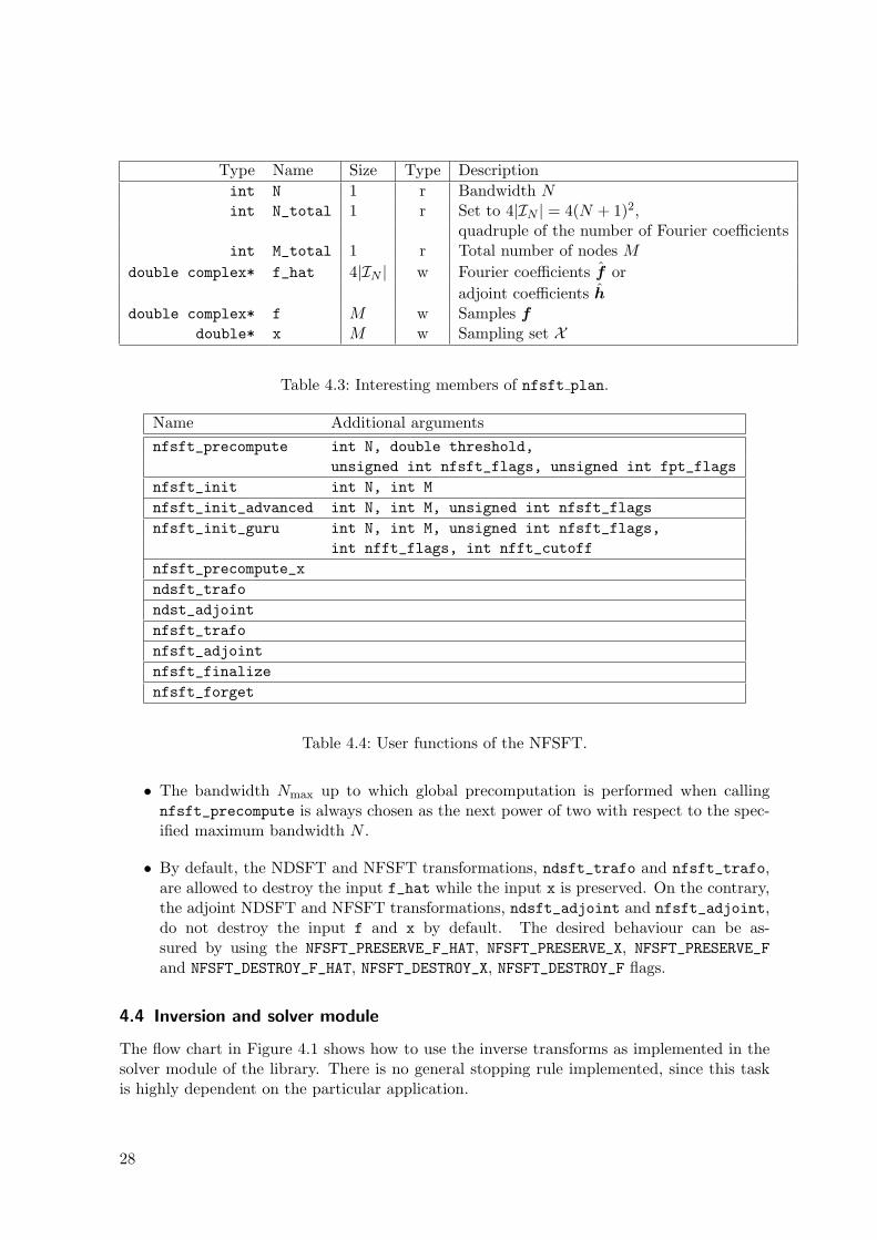
Type Name Size Type Descriptionint N 1 r Bandwidth Nint N_total 1 r Set to 4|IN | = 4(N + 1)2,

quadruple of the number of Fourier coefficientsint M_total 1 r Total number of nodes M

double complex* f_hat 4|IN | w Fourier coefficients f oradjoint coefficients h

double complex* f M w Samples fdouble* x M w Sampling set X

Table 4.3: Interesting members of nfsft plan.

Name Additional argumentsnfsft_precompute int N, double threshold,

unsigned int nfsft_flags, unsigned int fpt_flagsnfsft_init int N, int Mnfsft_init_advanced int N, int M, unsigned int nfsft_flagsnfsft_init_guru int N, int M, unsigned int nfsft_flags,

int nfft_flags, int nfft_cutoffnfsft_precompute_xndsft_trafondst_adjointnfsft_trafonfsft_adjointnfsft_finalizenfsft_forget

Table 4.4: User functions of the NFSFT.

• The bandwidth Nmax up to which global precomputation is performed when callingnfsft_precompute is always chosen as the next power of two with respect to the spec-ified maximum bandwidth N .

• By default, the NDSFT and NFSFT transformations, ndsft_trafo and nfsft_trafo,are allowed to destroy the input f_hat while the input x is preserved. On the contrary,the adjoint NDSFT and NFSFT transformations, ndsft_adjoint and nfsft_adjoint,do not destroy the input f and x by default. The desired behaviour can be as-sured by using the NFSFT_PRESERVE_F_HAT, NFSFT_PRESERVE_X, NFSFT_PRESERVE_Fand NFSFT_DESTROY_F_HAT, NFSFT_DESTROY_X, NFSFT_DESTROY_F flags.

4.4 Inversion and solver module

The flow chart in Figure 4.1 shows how to use the inverse transforms as implemented in thesolver module of the library. There is no general stopping rule implemented, since this taskis highly dependent on the particular application.

28

Initialise the Fourier transform.

Initialise the corresponding inverse.

Compute residuals.

Compute one iteration.

Finalise the inverse transform.

Finalise the Fourier transform.

?

?

?

?

?

��HHH

HHH

��

no yesStop?

?

-

Figure 4.1: Flow chart of the inverse transforms.

Each inverse transform basically wraps an already initialised Fourier transform. The userspecifies one of the Algorithms 5-8 by setting one of the flags (LANDWEBER, STEEPEST DESCENT,CGNR, CGNE). Weights and/or damping factors are used if the flags PRECOMPUTE WEIGHT,PRECOMPUTE DAMP are set and one has to initialise the members my iplan.w, my iplan.w hatin these cases. Default flags are CGNR.

In case of the NFFT, the library defines the structure infft plan. The members of thisplan are given by Table 4.5. The user functions for the inverse NFFT are collected in Table 4.6.They all have return type void and their first argument is of type infft plan*. Replacingnfft by any other Fourier transform gives the appropriate inverse to this transform.

29

Type Name Size Descriptiondouble* w M total weights w

double* w hat N total damping factors w

(FLT TYPE)* y M total right hand side y

(FLT TYPE)* f hat iter N total actual solution(FLT TYPE)* r iter M total residual vector rl+1

double dot r iter 1 ‖rl+1‖2W

Table 4.5: More important members of each inverse plan, where (FLT TYPE) is double for theNFCT and NFST and double complex in all other cases.

Name Additional argumentsinfft init nfft plan *mvinfft init advanced nfft plan *mv, unsigned infft flagsinfft before loopinfft loop one stepinfft finalize

Table 4.6: User functions of the inverse NFFT.

30

5 Examples

The library was tested on a AMD Athlon(tm) XP 2700+, 1GB memory, SuSe-Linux, kernel2.4.20-4GB-athlon, gcc version 3.3. In all tests with random input the nodes xj and theFourier coefficients fk are chosen pseudo randomly with xj ∈ [−0.5, 0.5]d and fk ∈ [0, 1] ×[0, 1]i.

5.1 Computing your first transform

The following code summarises the steps of Section 4.2 and computes a univariate NFFTfrom 14 Fourier coefficients and 19 nodes. Note that this routine is part of simple test.cin examples/nfft/ and uses additional routines as defined include/util.h to set up andshow vectors.

void simple_test_nfft_1d(){

nfft_plan p;int N=14;int M=19;

nfft_init_1d(&p,N,M);

nfft_vrand_shifted_unit_double(p.x,p.M_total);

if(p.nfft_flags & PRE_ONE_PSI)nfft_precompute_one_psi(&p);

nfft_vrand_unit_complex(p.f_hat,p.N_total);nfft_vpr_complex(p.f_hat,p.N_total,"given Fourier coefficients, f_hat");

ndft_trafo(&p);nfft_vpr_complex(p.f,p.M_total,"ndft, f");

nfft_trafo(&p);nfft_vpr_complex(p.f,p.M_total,"nfft, f");

nfft_finalize(&p);}

5.2 Computation time vs. problem size

The program nfft times in the same directory compares the computation time of the FFT([28], FFTW MEASURE), the straightforward evaluation of (2.2), denoted by NDFT, and theNFFT for increasing total problem sizes |IN | and space dimensions d = 1, 2, 3, where N =(N, . . . , N)>, N ∈ N. While the nodes for the FFT are restricted to the lattice N−1 � IN ,we choose M = Nd random nodes for the NDFT and the NFFT. Within the latter, we usethe oversampling factor σ = 2, the cut-off m = 4, and the Kaiser-Bessel window function

31

(PRE PSI, PRE PHI HUT). This results in a fixed accuracy of E∞ := ‖f − s‖∞/‖f‖1 ≈ 10−8

for d = 1, 2, 3.

lN FFT NDFT NFFT lN FFT NDFT NFFTd = 1 d = 2

3 1.3e− 07 8.7e− 06 4.6e− 06 6 9.9e− 07 5.7e− 04 3.2e− 044 2.0e− 07 3.5e− 05 8.7e− 06 8 4.4e− 06 9.2e− 03 1.3e− 035 4.0e− 07 1.4e− 04 1.7e− 05 10 2.1e− 05 1.5e− 01 5.2e− 036 8.9e− 07 5.6e− 04 3.6e− 05 12 1.2e− 04 2.4e+ 00 2.3e− 027 2.2e− 06 2.2e− 03 7.2e− 05 14 1.7e− 03 3.8e+ 01 1.5e− 018 4.8e− 06 9.0e− 03 1.4e− 04 16 2.1e− 02 * 6.8e− 019 1.1e− 05 3.6e− 02 2.9e− 04 18 8.4e− 02 * 2.8e+ 00

10 2.4e− 05 1.4e− 01 6.0e− 04 20 3.2e− 01 * 1.2e+ 0111 5.7e− 05 5.8e− 01 1.4e− 03 22 1.4e+ 00 * 5.3e+ 0112 1.5e− 04 2.3e+ 00 3.2e− 03 d = 313 5.5e− 04 9.4e+ 00 8.2e− 03 9 1.0e− 05 3.7e− 02 2.5e− 0214 1.7e− 03 3.8e+ 01 2.0e− 02 12 1.1e− 04 2.4e+ 00 2.5e− 0115 3.8e− 03 1.5e+ 02 4.9e− 02 15 3.4e− 03 1.5e+ 02 2.4e+ 0016 8.2e− 03 * 1.2e− 01 18 5.2e− 02 * 2.1e+ 0117 1.9e− 02 * 2.4e− 01 21 9.0e− 01 * 1.8e+ 0218 4.5e− 02 * 3.6e− 0119 9.2e− 02 * 9.8e− 0120 1.9e− 01 * 2.1e+ 0021 4.2e− 01 * 4.2e+ 0022 1.0e− 00 * 9.5e+ 00

Table 5.1: Computation time in seconds with respect to lN = log2 |IN |. Note that we used ac-cumulated measurements in case of small times and the times (*) are not displayeddue to the large response time in comparison to the FFT time.

We conclude the following: The FFT and the NFFT show the expected O(|IN | log |IN |)time complexity, i.e., doubling the total size |IN | results in only slightly more than twicethe computation time, whereas the NDFT behaves as O(|IN |2). Note furthermore, that theconstant in the O-notation is independent of the space dimension d for the FFT and theNDFT, whereas the computation time of the NFFT increases considerably for larger d.

5.3 Accuracy vs. window function and cut-off parameter m

The accuracy of the Algorithm 1, measured by

E2 =‖f − s‖2

‖f‖2=

M−1∑j=0

|fj − s (xj) |2/M−1∑j=0

|fj |2 1

2

andE∞ =

‖f − s‖∞‖f‖1

= max0≤j<M

|fj − s (xj) |/∑

k∈IN

|fk|

is shown in Figure 5.1.

32

0 5 10 1510

−15

10−10

10−5

100

0 5 10 1510

−15

10−10

10−5

100

0 5 10 1510

−15

10−10

10−5

100

0 5 10 1510

−15

10−10

10−5

100

0 5 10 1510

−15

10−10

10−5

100

0 5 10 1510

−15

10−10

10−5

100

Figure 5.1: The error E2 (top) and E∞ (bottom) with respect to m, from left to right d =1, 2, 3 (N = 212, 26, 24, σ = 2, M = 10000), for Kaiser Bessel- (circle), Sinc- (x),B-Spline- (+), and Gaussian window (triangle).

5.4 Computing an inverse transform

The usage of the inverse NFFT is demonstrated by simple test in examples/solver. Exe-cuting the MatLab script glacier.m in the same directory produces the following two plots.Note that the corresponding C-file glacier.c is called from the MatLab script.

Figure 5.2: Reconstruction of the glacier from samples at M = 8345 nodes (vol87.dat from[27]) with N0 = N1 = 256 and 40 iterations.

33

6 Applications

In this section we describe important applications which are based on the NFFT kernel. Onecan find these programs in the directory applications.

6.1 Summation of smooth and singular kernels

We are interested in the fast evaluation of linear combinations of radial functions, i.e. thecomputation of

g(yj

):=

N∑k=1

αkK(∥∥yj − xk

∥∥2

)for j = 1, . . . ,M and nodes xk,yj ∈ Rd. For smooth kernels K with an additional parameterc > 0, e.g. the Gaussian K(x) = e−x2/c2 , the multiquadric K(x) =

√x2 + c2 or the inverse

multiquadric K(x) = 1/√x2 + c2 our algorithm requires O(N + M) arithmetic operations.

In the case of singular kernels K, e.g.,

1x2,

1|x|, log |x|, x2 log |x|, 1

x,

sin(cx)x

,cos(cx)x

, cot(cx)

an additional regularisation procedure must be incorporated and the algorithm has the arith-metic complexity O(N logN + M) or O(M logM + N) if either the target nodes yj or thesource nodes xk are “reasonably uniformly distributed”.

Note that the proposed fast algorithm [49, 50, 23] generalises the diagonalisation of convo-lution matrices by Fourier matrices to the setting of arbitrary nodes. In particular, this yieldsnearly the same arithmetic complexity as the FMM [5] while allowing for an easy change ofvarious kernels. A recent application in particle simulation is given in [43]. The directoryapplications/fastsum contains C and MatLab programs that show how to use the fastsummation method.

6.2 Fast Gauss transform

This is a special case of the fast summation method, we compute approximations of thefollowing sums. Given complex coefficients αk ∈ C and source nodes xk ∈ [−1

4 ,14 ], our goal

consists in the fast evaluation of the sum

g (y) =N∑

k=1

αke−σ|y−xk|2

at the target nodes yj ∈ [−14 ,

14 ], j = 1, . . . ,M , where σ = a + ib, a > 0, b ∈ R, denotes

a complex parameter. For details see [37] and the related paper [2] for applications. Allnumerical examples of [37] are produced by the programs in applications/fastgauss.

6.3 Summation of zonal functions on the sphere

Given M,N ∈ N, arbitrary source nodes ηk ∈ S2 and real coefficients αk ∈ R, evaluate thesum

g (ξ) :=N∑

k=1

αkK (ηk · ξ)

34

at the target nodes ξj ∈ S2, j = 1, . . . ,M . The naive approach for evaluating this sum takesO(MN) floating point operations if we assume that the zonal function K can be evaluatedin constant time or that all values K(ηk · ξj) can be stored in advance.

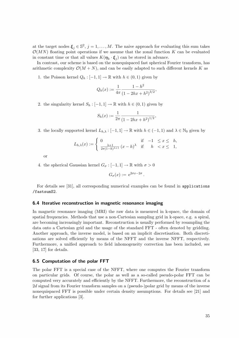
In contrast, our scheme is based on the nonequispaced fast spherical Fourier transform, hasarithmetic complexity O(M +N), and can be easily adapted to such different kernels K as

1. the Poisson kernel Qh : [−1, 1] → R with h ∈ (0, 1) given by

Qh(x) :=14π

1− h2

(1− 2hx+ h2)3/2,

2. the singularity kernel Sh : [−1, 1] → R with h ∈ (0, 1) given by

Sh(x) :=12π

1

(1− 2hx+ h2)1/2,

3. the locally supported kernel Lh,λ : [−1, 1] → R with h ∈ (−1, 1) and λ ∈ N0 given by

Lh,λ(x) :=

{0 if −1 ≤ x ≤ h,

λ+12π(1−h)λ+1 (x− h)λ if h < x ≤ 1,

or

4. the spherical Gaussian kernel Gσ : [−1, 1] → R with σ > 0

Gσ(x) := e2σx−2σ .

For details see [31], all corresponding numerical examples can be found in applications/fastsumS2.

6.4 Iterative reconstruction in magnetic resonance imaging

In magnetic resonance imaging (MRI) the raw data is measured in k-space, the domain ofspatial frequencies. Methods that use a non-Cartesian sampling grid in k-space, e.g. a spiral,are becoming increasingly important. Reconstruction is usually performed by resampling thedata onto a Cartesian grid and the usage of the standard FFT - often denoted by gridding.Another approach, the inverse model, is based on an implicit discretisation. Both discreti-sations are solved efficiently by means of the NFFT and the inverse NFFT, respectively.Furthermore, a unified approach to field inhomogeneity correction has been included, see[33, 17] for details.

6.5 Computation of the polar FFT

The polar FFT is a special case of the NFFT, where one computes the Fourier transformon particular grids. Of course, the polar as well as a so-called pseudo-polar FFT can becomputed very accurately and efficiently by the NFFT. Furthermore, the reconstruction of a2d signal from its Fourier transform samples on a (pseudo-)polar grid by means of the inversenonequispaced FFT is possible under certain density assumptions. For details see [21] andfor further applications [3].

35


In magnetic resonance imaging (MRI) the raw data is measured in k-space, the domain ofspatial frequencies. Methods that use a non-Cartesian (e.g. spiral) sampling grid in k-spaceare becoming increasingly important. Reconstruction is usually performed by resampling thedata onto a Cartesian grid and use the standard FFT. This model is called gridding. Anotherapproach, the inverse model, is based on an implicit discretisation. The gridding model isthe explicit computation of the picture with given Fourier samples. The inverse model is theimplicit computation. We solve both by using the NFFT and the iNFFT for both approaches.Furthermore we are able to give a unified approach to the field inhomogeneity correction. Fordetails see [33, 14].


The polar FFT is a special case of the NFFT, where we compute the Fourier transform onspecial grids. We show that the polar as well as the pseudo-polar FFT can be computed veryaccurately and efficiently by the NFFT. Furthermore, we discuss the reconstruction of a 2dsignal from its Fourier transform samples on a (pseudo-)polar grid by means of the inversenonequispaced FFT. For details see [18] and for further applications [2].

−0.5 0 0.5−0.5

0

0.5

−0.5 0 0.5−0.5

0

0.5

−0.5 0 0.5−0.5

0

0.5

Figure 9.1: Left to right: polar, modified polar, and linogram grid of size R = 16, T = 32.

9.6 Radon transform and computer tomography

We are interested in efficient and high quality reconstructions of digital N×N medical imagesfrom their Radon transform. The standard reconstruction algorithm, the filtered backprojec-tion, ensures a good quality of the images at the expense of O(N3) arithmetic operations.Fourier reconstruction methods reduce the number of arithmetic operations to O(N2 logN).Unfortunately, the straightforward Fourier reconstruction algorithm suffers from unacceptableartifacts so that it is useless in practice. A better quality of the reconstructed images can beachieved by our algorithm based on NFFTs. For details see [45, 44, 46].

9.7 Ridgelet transform

Ridgelets have been designed by Cand‘es et. all. (see e.g. [10]) to deal with line singularitieseffectively by mapping them into point singularities using the Radon transform.

The discrete ridgelet transform is designed by first using a discrete Radon transform basedon NFFT and then applying a dual-tree complex wavelet transform.

37





−0.5 0 0.5−0.5

0

0.5

−0.5 0 0.5−0.5

0

0.5

−0.5 0 0.5−0.5

0

0.5







37





−0.5 0 0.5−0.5

0

0.5

−0.5 0 0.5−0.5

0

0.5

−0.5 0 0.5−0.5

0

0.5







37


6.6 Radon transform, computer tomography, and ridgelet transform

We are interested in efficient and high quality reconstructions of digital N×N medical imagesfrom their Radon transform. The standard reconstruction algorithm, the filtered backprojec-tion, ensures a good quality of the images at the expense of O(N3) arithmetic operations.Fourier reconstruction methods reduce the number of arithmetic operations to O(N2 logN).Unfortunately, the straightforward Fourier reconstruction algorithm suffers from unacceptableartifacts so that it is useless in practice. A better quality of the reconstructed images canbe achieved by our algorithm based on NFFTs. For details see [47, 46, 48] and the directoryapplications/radon.

Another application of the discrete Radon transform is the discrete Ridgelet transform, seee.g. [10]. A simple test program for denoising an image by hard thresholding the ridgeletcoefficients can be found in applications/radon. It uses the NFFT-based discrete Radontransform and the translation-invariant discrete Wavelet transform based on MatLab toolboxWaveLab850 [11]. See [39] for details.

References

[1] C. Anderson and M. Dahleh. Rapid computation of the discrete Fourier transform. SIAMJ. Sci. Comput., 17:913 – 919, 1996.

[2] F. Andersson and G. Beylkin. The fast Gauss transform with complex parameters. J.Comput. Physics, 203:274 – 286, 2005.

[3] A. Averbuch, R. Coifman, D. L. Donoho, M. Elad, and M. Israeli. Fast and accuratepolar Fourier transform. Appl. Comput. Harmon. Anal., 21:145 – 167, 2006.

[4] R. F. Bass and K. Grochenig. Random sampling of multivariate trigonometric polyno-mials. SIAM J. Math. Anal., 36:773 – 795, 2004.

[5] R. K. Beatson and L. Greengard. A short course on fast multipole methods. InM. Ainsworth, J. Levesley, W. A. Light, and M. Marletta, editors, Wavelets, MultilevelMethods and Elliptic PDEs. Clarendon Press, 1997.

[6] P. J. Beatty, D. G. Nishimura, and J. M. Pauly. Rapid gridding reconstruction with aminimal oversampling ratio. IEEE Trans. Med. Imag., 24:799 – 808, 2005.

36

[7] G. Beylkin. On the fast Fourier transform of functions with singularities. Appl. Comput.Harmon. Anal., 2:363 – 381, 1995.

[8] A. Bjorck. Numerical Methods for Least Squares Problems. SIAM, Philadelphia, 1996.

[9] H.-J. Bungartz and M. Griebel. Sparse grids. Acta Numer., 13:147 – 269, 2004.

[10] E. J. Candes, L. Demanet, D. L. Donoho, and L. Ying. Fast discrete curvelet transforms.SIAM Multiscale Model. Simul., 3:861 – 899, 2006.

[11] D. Donoho, A. Maleki, and M. Shaharam. Wavelab 850. http://www-stat.stanford.edu/∼wavelab, 2006.

[12] J. R. Driscoll and D. Healy. Computing Fourier transforms and convolutions on the2–sphere. Adv. in Appl. Math., 15(2):202 – 250, 1994.

[13] J. R. Driscoll, D. Healy, and D. Rockmore. Fast discrete polynomial transforms withapplications to data analysis for distance transitive graphs. SIAM J. Comput., 26:1066– 1099, 1996.

[14] A. J. W. Duijndam and M. A. Schonewille. Nonuniform fast Fourier transform. Geo-physics, 64:539 – 551, 1999.

[15] A. Dutt and V. Rokhlin. Fast Fourier transforms for nonequispaced data. SIAM J. Sci.Stat. Comput., 14:1368 – 1393, 1993.

[16] A. Dutt and V. Rokhlin. Fast Fourier transforms for nonequispaced data II. Appl.Comput. Harmon. Anal., 2:85 – 100, 1995.

[17] H. Eggers, T. Knopp, and D. Potts. Field inhomogeneity correction based on griddingreconstruction. Preprint 06-10, TU-Chemnitz, 2006.

[18] B. Elbel and G. Steidl. Fast Fourier transform for nonequispaced data. In C. K. Chuiand L. L. Schumaker, editors, Approximation Theory IX, Nashville, 1998. VanderbiltUniversity Press.

[19] H. G. Feichtinger, K. Grochenig, and T. Strohmer. Efficient numerical methods in non-uniform sampling theory. Numer. Math., 69:423 – 440, 1995.

[20] M. Fenn, S. Kunis, and D. Potts. Fast evaluation of trigonometric polynomials fromhyperbolic crosses. Numer. Algorithms, 41:339 – 352, 2006.

[21] M. Fenn, S. Kunis, and D. Potts. On the computation of the polar FFT. Appl. Comput.Harmon. Anal., to appear.

[22] M. Fenn and D. Potts. Fast summation based on fast trigonometric transforms at noneq-uispaced nodes. Numer. Linear Algebra Appl., 12:161 – 169, 2005.

[23] M. Fenn and G. Steidl. Fast NFFT based summation of radial functions. SamplingTheory in Signal and Image Processing, 3:1 – 28, 2004.

[24] J. A. Fessler and B. P. Sutton. Nonuniform fast Fourier transforms using min-maxinterpolation. IEEE Trans. Signal Process., 51:560 – 574, 2003.

37

[25] K. Fourmont. Schnelle Fourier–Transformation bei nichtaquidistanten Gittern und to-mographische Anwendungen. Dissertation, Universitat Munster, 1999.

[26] K. Fourmont. Non equispaced fast Fourier transforms with applications to tomography.J. Fourier Anal. Appl., 9:431 – 450, 2003.

[27] R. Franke. http://www.math.nps.navy.mil/∼rfranke/README.

[28] M. Frigo and S. G. Johnson. FFTW, C subroutine library. http://www.fftw.org.

[29] L. Greengard and J.-Y. Lee. Accelerating the nonuniform fast Fourier transform. SIAMRev., 46:443 – 454, 2004.

[30] J. I. Jackson, C. H. Meyer, D. G. Nishimura, and A. Macovski. Selection of a convolutionfunction for Fourier inversion using gridding. IEEE Trans. Med. Imag., 10:473 – 478,1991.

[31] J. Keiner, S. Kunis, and D. Potts. Fast summation of Radial Functions on the Sphere.Computing, 78(1):1–15, 2006.

[32] J. Keiner and D. Potts. Fast evaluation of quadrature formulae on the sphere. PreprintA-06-07, Universitat zu Lubeck, 2006.

[33] T. Knopp, S. Kunis, and D. Potts. Fast iterative reconstruction for MRI from nonuniformk-space data. revised Preprint A-05-10, Universitat zu Lubeck, 2005.

[34] S. Kunis and D. Potts. Fast spherical Fourier algorithms. J. Comput. Appl. Math.,161(1):75 – 98, 2003.

[35] S. Kunis and D. Potts. Stability results for scattered data interpolation by trigonometricpolynomials. revised Preprint A-04-12, Universitat zu Lubeck, 2004.

[36] S. Kunis and D. Potts. Time and memory requirements of the nonequispaced FFT.Preprint 06-01, TU-Chemnitz, 2006.

[37] S. Kunis, D. Potts, and G. Steidl. Fast Gauss transform with complex parameters usingNFFTs. J. Numer. Math., to appear.

[38] J.-Y. Lee and L. Greengard. The type 3 nonuniform FFT and its applications. J. Comput.Physics, 206:1 – 5, 2005.

[39] J. Ma and M. Fenn. Combined complex ridgelet shrinkage and total variation minimiza-tion. SIAM J. Sci. Comput., 28:984–1000, 2006.

[40] N. Nguyen and Q. H. Liu. The regular Fourier matrices and nonuniform fast Fouriertransforms. SIAM J. Sci. Comput., 21:283 – 293, 1999.

[41] A. Nieslony and G. Steidl. Approximate factorizations of Fourier matrices with noneq-uispaced knots. Linear Algebra Appl., 266:337 – 351, 2003.

[42] J. Pelt. Fast computation of trigonometric sums with applications to frequency analysisof astronomical data. In D. Maoz, A. Sternberg, and E. Leibowitz, editors, AstronomicalTime Series, pages 179 – 182, Kluwer, 1997.

38

[43] G. Poplau, D. Potts, and U. van Rienen. Calculation of 3d space-charge fields of bunchesof charged particles by fast summation. In Proceedings of SCEE 2004 (5th InternationalWorkshop on Scientific Computing in Electrical Engineering, 2005.

[44] D. Potts. Fast algorithms for discrete polynomial transforms on arbitrary grids. LinearAlgebra Appl., 366:353 – 370, 2003.

[45] D. Potts. Schnelle Fourier-Transformationen fur nichtaquidistante Daten und Anwen-dungen. Habilitation, Universitat zu Lubeck, 2003.

[46] D. Potts and G. Steidl. New Fourier reconstruction algorithms for computerized tomog-raphy. In A. Aldroubi, A. Laine, and M. Unser, editors, Proceedings of SPIE: WaveletApplications in Signal and Image Processing VIII, volume 4119, pages 13 – 23, 2000.

[47] D. Potts and G. Steidl. A new linogram algorithm for computerized tomography. IMAJ. Numer. Anal., 21:769 – 782, 2001.

[48] D. Potts and G. Steidl. Fourier reconstruction of functions from their nonstandardsampled Radon transform. J. Fourier Anal. Appl., 8:513 – 533, 2002.

[49] D. Potts and G. Steidl. Fast summation at nonequispaced knots by NFFTs. SIAM J.Sci. Comput., 24:2013 – 2037, 2003.

[50] D. Potts, G. Steidl, and A. Nieslony. Fast convolution with radial kernels at nonequis-paced knots. Numer. Math., 98:329 – 351, 2004.

[51] D. Potts, G. Steidl, and M. Tasche. Fast algorithms for discrete polynomial transforms.Math. Comput., 67(224):1577 – 1590, 1998.

[52] D. Potts, G. Steidl, and M. Tasche. Fast Fourier transforms for nonequispaced data: Atutorial. In J. J. Benedetto and P. J. S. G. Ferreira, editors, Modern Sampling Theory:Mathematics and Applications, pages 247 – 270. Birkhauser, Boston, 2001.

[53] R. A. Scramek and F. R. Schwab. Imaging. In R. Perley, F. R. Schwab, and A. Bridle,editors, Astronomical Society of the Pacific Conference, volume 6, pages 117 – 138, 1988.

[54] F. Sprengel. A class of function spaces and interpolation on sparse grids. Numer. Funct.Anal. Optim., 21:273 – 293, 2000.

[55] G. Steidl. A note on fast Fourier transforms for nonequispaced grids. Adv. Comput.Math., 9:337 – 353, 1998.

[56] B. Tian and Q. H. Liu. Nonuniform fast cosine transform and Chebyshev PSTD algo-rithm. J. Electromagnet. Waves Appl, 14:797 – 798, 2000.

[57] A. F. Ware. Fast approximate Fourier transforms for irregularly spaced data. SIAMRev., 40:838 – 856, 1998.

[58] C. Zenger. Sparse grids. In Parallel algorithms for partial differential equations (Kiel,1990), volume 31 of Notes Numer. Fluid Mech., pages 241–251. Vieweg, Braunschweig,1991.

39

nfft 3.0 - tutorial - tu chemnitzpotts/nfft/guide/nfft3.pdf · this tutorial surveys the fast...

Documents