GEOLOGI FOR SAMFUNNETGEOLOGY FOR SOCIETY

NGUNorges geologiske undersøkelseGeological Survey of Norway

Geological Survey ofPostboks 6315 SluppenNO-7491 Trondheim, NorwayTel.: 47 73 90 40 00Telefax 47 73 92 16 20

Report no.: 2014.007Title:Helicopter-borne magnetic and radiometric geophysicalHadseløya areas, in Troms and NordlandAuthors:

Alexandros Stampolidis, Frode Ofstad and VikasBaranwalCounty:

Nordland and Troms

Map-sheet name (M=1:250.000)

Narvik and Svolvær

Deposit name and grid-reference: HinnøyaWGS 84, UTM zone 33W, 530000 E, 7600000 NFieldwork carried out:

July-August 2013Date of report:

March

Summary:NGU conducted an airborne

Tjeldøya and Hadseløya islands, in Troms and Nordlandthe MINN project (Mineral resources in Northern Norway)acquisition, processing and visualization of recorded datasets. The geophysical survey results reportedherein are approximately 8100 line km, covering an area of

Two helicopter-borne systems were used in this survey. More than 95% of thedone with a helicopter-borne system that was designed to obtainradiometric data. It had a Scintrex Csspectrometer installed under the helicopterScintrex Cs-2 for the magnetic field recordingsgamma-rays installed under the helicopter.

The entire survey was flown with 200 m line spacingbut Hadseløya and Nipa, a small part of the western Hinnøya, were flown at 140respectively. The average speed75 km/h, depending mainly on the local topographywhole survey was about 75 m.

Collected data were processed at NGU using Geosoft Oasis Montaj software. Raw total magneticfield data were corrected for diurnalRadiometric data were processed using standard procedures recommended by International AtomicEnergy Association.

Data were gridded with a cell size of 50 x 50 m and presented as shaded rel1:50.000 (Hadseløya) and1:80.000 (Austavågøya, Hinnøya, Tieldøya)

Keywords:

Magnetic

Geological Survey of NorwayPostboks 6315 Sluppen

7491 Trondheim, NorwayTel.: 47 73 90 40 00Telefax 47 73 92 16 20 REPORT

ISSN 0800-3416 Grading: Open

and radiometric geophysical survey at Austvågøya, Hinnøya, TjeldøyaNordland counties.

, Frode Ofstad and VikasClient:

NGU

Municipalities:

Tjeldsund, Lødingen, Sortland, Hadsel og Vågan

Map-sheet no. and -name (M=1:50.000)1331 IV Evenes 1332 III Tjeldsundet 1231 I Lødingen1231 IV Raftsundet, 1232 II1132 II Stokmarknes, 1131

HinnøyaUTM zone 33W, 530000 E, 7600000 N

Number of pages: 36 Price (NOK):Map enclosures:

Date of report:

March 10th 2014Project no.:

342900

NGU conducted an airborne magnetic and radiometric survey over theislands, in Troms and Nordland counties between July

(Mineral resources in Northern Norway). This report describes and documents theion, processing and visualization of recorded datasets. The geophysical survey results reported

line km, covering an area of approximately 1620

borne systems were used in this survey. More than 95% of theborne system that was designed to obtain detailed airborne magnetic and

had a Scintrex Cs-3 magnetometer in a towed bird andinstalled under the helicopter belly. The other helicopter-borne

2 for the magnetic field recordings and a similar 1024 channels RSXinstalled under the helicopter.

survey was flown with 200 m line spacing. The main flight line directionbut Hadseløya and Nipa, a small part of the western Hinnøya, were flown at 140

average speed over different parts of the surveyed areas ranged, depending mainly on the local topography. The average terrain clearance of the bird

Collected data were processed at NGU using Geosoft Oasis Montaj software. Raw total magneticfield data were corrected for diurnal variations and levelled using standard microRadiometric data were processed using standard procedures recommended by International Atomic

cell size of 50 x 50 m and presented as shaded rel(Hadseløya) and1:80.000 (Austavågøya, Hinnøya, Tieldøya).

Geophysics Airborne

Radiometric Technical report

REPORT

at Austvågøya, Hinnøya, Tjeldøya and

Tjeldsund, Lødingen, Sortland, Hadsel og Vågan

name (M=1:50.000)1331 IV Evenes 1332 III Tjeldsundet 1231 I Lødingen

II Gullesfjorden 1232 III SortlandI Austvågøya

Price (NOK): 140,-

Person responsible:

over the Austvågøya, Hinnøya,counties between July-August 2013 as a part of

. This report describes and documents theion, processing and visualization of recorded datasets. The geophysical survey results reported

approximately 1620 km2.

borne systems were used in this survey. More than 95% of the measurements wereed airborne magnetic and

and a 1024 channels RSX-5system was similar, had a

1024 channels RSX-5 spectrometer for

line direction was 90o (E-W),but Hadseløya and Nipa, a small part of the western Hinnøya, were flown at 140o and 145o (NNE-SSW),

over different parts of the surveyed areas ranged daily between 50 and. The average terrain clearance of the bird for the

Collected data were processed at NGU using Geosoft Oasis Montaj software. Raw total magneticand levelled using standard micro-levelling algorithm.

Radiometric data were processed using standard procedures recommended by International Atomic

cell size of 50 x 50 m and presented as shaded relief maps at scales of

Airborne

Technical report

Table of Contents

1. INTRODUCTION........................................................................................................ 5

2. SURVEY SPECIFICATIONS.................................................................................... 6

2.1 Airborne Survey Parameters ....................................................................................... 6

2.2 Airborne Survey Instrumentation ............................................................................... 9

2.3 Airborne Survey Logistics Summary .......................................................................... 9

3. DATA PROCESSING AND PRESENTATION .................................................... 11

3.1 Total Field Magnetic Data.......................................................................................... 11

3.2 Radiometric data ......................................................................................................... 13

4. PRODUCTS ................................................................................................................ 17

5. REFERENCES ........................................................................................................... 18

APPENDIX A1: FLOW CHART OF MAGNETIC PROCESSING ................................................. 19APPENDIX A2: DESCRIPTION OF THE MATLAB CODE ....................................................... 19APPENDIX A3: FLOW CHART OF RADIOMETRY PROCESSING ............................................ 19

TABLES

Table 1. Flight specifications of the surveyed areas.............................................................. 5Table 2. Base station magnetometer locations (WGS-84, UTM-zone 33N) ........................ 7Table 3. Instrument Specifications ......................................................................................... 9Table 4. Survey Specifications Summary............................................................................... 9Table 5. Specified channel windows for the 1024 RSX-5 systems used in this survey..... 13Table 6. List of Geosoft XYZ files available from NGU on request. ................................. 17Table 7. Maps available from NGU on request. .................................................................. 17

4

FIGURES

Figure 1: Surveyed areas.. .................................................................................................................... 5Figure 2: Base station magnetometer locations .................................................................................. 7Figure 3: A base station magnetometer (GEM GSM-19) .................................................................. 8Figure 4: The first helicopter used in survey. ................................................................................... 10Figure 5: The second helicopter used in survey................................................................................ 10Figure 6: An example of Gamma-ray spectrum............................................................................... 13Figure 7: Total Magnetic Field anomaly Austvågøya-Hinnøya-Tjeldøya...................................... 21Figure 8: Magnetic Vertical Gradient Austvågøya-Hinnøya-Tjeldøya.......................................... 22Figure 9: Magnetic Horizontal Gradient Austvågøya-Hinnøya-Tjeldøya ..................................... 23Figure 10: Magnetic Tilt Derivative Austvågøya-Hinnøya-Tjeldøya ............................................. 24Figure 11: Total Magnetic Field anomaly Hadseløya ...................................................................... 25Figure 12: Magnetic Vertical Gradient Hadseløya .......................................................................... 26Figure 13: Magnetic Horizontal Gradient Hadseløya...................................................................... 27Figure 14: Magnetic Tilt Derivative Hadseløya................................................................................ 28Figure 15: Uranium Ground Concentration Austvågøya-Hinnøya-Tjeldøya ............................... 29Figure 16: Thorium Ground Concentration Austvågøya-Hinnøya-Tjeldøya................................ 30Figure 17: Potassium Ground Concentration Austvågøya-Hinnøya-Tjeldøya ............................. 31Figure 18: Ternary Image of Radiation Concentrations Austvågøya-Hinnøya-Tjeldøya............ 32Figure 19: Uranium Ground Concentration Hadseløya.................................................................. 33Figure 20: Thorium Ground Concentration Hadseløya .................................................................. 34Figure 21: Potassium Ground Concentration Hadseløya................................................................ 35Figure 22: Ternary Image of Radiation Concentrations Hadseløya .............................................. 36

5

1. INTRODUCTION

Recognising the impact that investment in mineral exploration and mining can have on thesocio-economic situation of a region, the government of Norway initiated the MINN program(Mineral resources in North Norway). The goal of this program is to enhance the geologicalinformation that is relevant to an assessment of the mineral potential of the three northernmostcounties. The airborne geophysical surveys - helicopter borne and fixed wing- are importantintegral parts of MINN program. The airborne survey results reported herein amount about8100 line km (1620 km2) over the surveyed areas, as shown in Figure 1.

The surveyed area was divided into five sub-regions during the acquisition period. Area A isHadseløya island and was flown at a NNW-SSE direction (140o). Area B eastern part ofAustvågøya, area C southern part of Hinnøya, and D Tjeldøya island were flown at an East-West direction (90o). The last sub-region, E, is the small area called Nipa. It was flown by adifferent helicopter-borne system than the previous four areas, at a NNW-SSE direction(145o).

Table 1. Flight specifications of the surveyed areasSub-

regionName Surveyed

lines (km)Surveyed

area (Km2)Flightdirection

Average flightspeed (km/h)

A Hadseløya 535 103 NNW-SSE 60

B Austvågøya/Hinnøya 1913 378 E-W 53C Hinnøya 4577 925 E-W 75D Tjeldøya 970 190 E-W 70

E Nipa 102 21 NNW-SSE 50Total 8097 1617

Figure 1: Surveyed areas. A. Hadseløya area (red line), B. Austvågøya/Hinnøya area (blue line), C.Hinnøya area (green line), D. Tjeldøya area (black line) and E. Nipa area (brown line).

6

The objective of the airborne geophysical survey was to obtain a dense high-resolution aero-magnetic and radiometric data set over the survey area. These data sets are required for theenhancement of a general understanding of the regional geology of the area. In this regard, thedata can also be used to map contacts and structural features within the area. It also improvesdefining the potential of known zones of mineralization, their geological settings, andidentifying new areas of interest.

The survey incorporated the use of a high-sensitivity Cesium magnetometers, gamma-rayspectrometers and radar altimeters. GPS navigation computer systems with flight pathindicators ensured accurate positioning of the geophysical data with respect to the WorldGeodetic System 1984 geodetic datum (WGS-84).

2. SURVEY SPECIFICATIONS

2.1 Airborne Survey Parameters

NGU used two helicopter-borne systems for the purposes of this survey.

The first system (fig. 4) had a optically pumped Cesium magnetometer (Cs-2) towed 30 meterbelow the helicopter for the magnetic field recordings and a 1024 channel RSX-5 gamma-rayspectrometer fixed under the belly of the helicopter to map ground concentrations ofUranium, Thorium and Potassium. This system was used to measure Nipa (sub-region E in fig1.) and a few survey lines in Tjeldøya (sub-region D in fig 1.), and is described in more detailsin other NGU reports (i.e NGU Report 2013.047)

The second system (fig. 5), that made more than 95% of the measurements in this survey, is ahelicopter-borne system that was designed to obtain detailed airborne magnetic andradiometric data. This system used a Scintrex Cs-3 housed in a 2 m long bird, towed 15meters below the helicopter for the magnetic field recordings and a similar 1024 channelgamma-ray spectrometer to the one that was installed on the first system, to map groundconcentrations of Uranium, Thorium and Potassium.

The airborne survey began on July 14th and ended on August 30th, 2013. A EurocopterAS350-B2 from helicopter company HeliScan AS was used for the major part of the survey,while a Eurocopter AS350-B3 employed to fly over Nipa and some lines in Tjeldøya. Thesurvey lines were spaced 200 m apart throughout the survey, but the fight direction wasdiffering in some sub-regions as shown on Table 1. Instrument operation was performed byHeliscan AS employees.

Large water bodies, rugged terrain and abrupt changes in topography affected the pilot’sability to ‘drape’ the terrain; therefore there are positive and negative variations in sensorheight with respect to the standard helicopter height, which is defined as 60 m plus a height ofobstacles (trees, power lines). The average survey height for the magnetometer was about55m for the first system and about 80 m for the second system, while the spectrometer was atabout 85m for the first system and about 95 m for the second system. Due to bad weatherconditions in the acquisition period and the flight safety rules, parts of some profiles wereflown at high altitudes. These data were discarded during the radiometric processing.

The ground speed of the aircraft varied from 40 – 120 km/h depending on topography, winddirection and its magnitude. On average the ground speed during the whole survey was about70 km/h. The average ground speeds for each sub-region are given in Table 1.

7

Magnetic data were recorded at 0.2 second intervals resulting in approximately 4 m pointspacing. Spectrometry data was recorded every 1 second giving a point spacing ofapproximately 20 meters.

The above parameters were designed to allow for sufficient detail in the data to detect subtleanomalies that may represent mineralization and/or rocks of different lithological and petro-physical composition.

Figure 2: Base station magnetometer locations

A base magnetometer to monitor diurnal variations in the magnetic field, was installed closeto the helicopter base during the whole survey period. The rough topography and theproximity to the areas under investigation impose changes to the helicopter base location, andtherefore changes to the base magnetometer locations which are depicted on figure 2. Namesand locations of the base magnetometer stations are given in Table 2.

Table 2. Base station magnetometer locations (WGS-84, UTM-zone 33N)Base mag

nameLocation UTM E

(m)UTM N

(m)Instrument Sampling

interval (sec)

BM1 Sortland 515050 7617050 GEM GSM-19 3

BM2 Sortland 511060 7614250 GEM GSM-19 3

BM3 Sortland 508150 7612860 GEM GSM-19 3

BM4 Svolvær 485940 7570150 GEM GSM-19 3

BM5 Bogen 581830 7603200 GEM GSM-19Scintrex CS3

31

8

A GEM GSM-19 base station magnetometer was used to record data every 3 seconds. TheCPU clock of the magnetometer was synchronized through the built-in GPS receiver to permitsubsequent removal of diurnal drift. During the last day of the acquisition a Scintrex Cs-3magnetometer was used as base station instead. In order to bring the data from different basestations to the same level, complete recordings from the Andenes Observatory (540960E,7687640N), for the whole period of the survey, were used as reference. The variations in therecorded magnetic field at the base stations were similar to those recorded at the magneticobservatory of Andenes, which lies just 70 km north of the surveyed area.

Figure 3: A base station magnetometer (GEM GSM-19) installed 8.5 km southwest of Sortland

Navigation system uses GPS/GLONASS satellite tracking systems to provide real-time WGS-84 coordinate locations for every second. The accuracy achieved with no differentialcorrections is reported to be 5 m in the horizontal directions. The GPS receiver antenna wasmounted externally to the tail tip of the helicopter.

For quality control, the magnetic, radiometric, altitude and navigation data were monitored ontwo separate windows in the operator's display during flight while they were recorded inASCII data streams to the acquisition PC hard disk drive.

9

2.2 Airborne Survey Instrumentation

Instrument specifications are given in table 3.

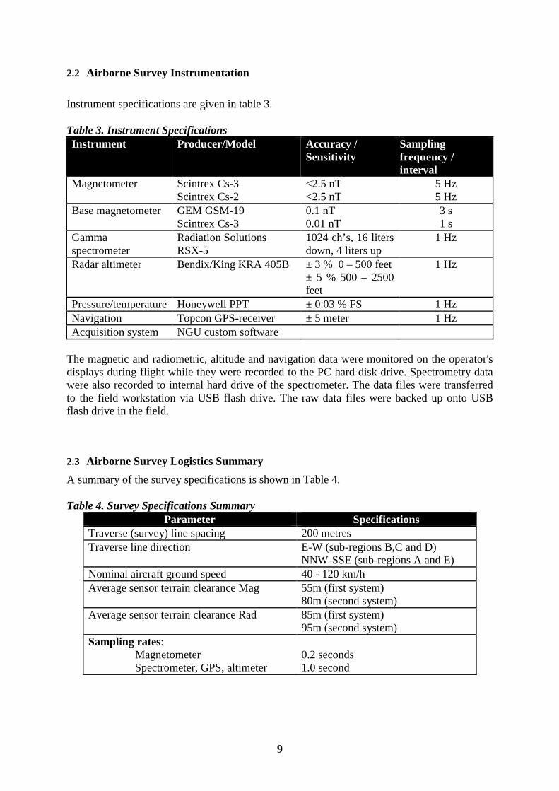
Table 3. Instrument SpecificationsInstrument Producer/Model Accuracy /

SensitivitySamplingfrequency /interval

Magnetometer Scintrex Cs-3Scintrex Cs-2

<2.5 nT<2.5 nT

5 Hz5 Hz

Base magnetometer GEM GSM-19Scintrex Cs-3

0.1 nT0.01 nT

3 s1 s

Gammaspectrometer

Radiation SolutionsRSX-5

1024 ch’s, 16 litersdown, 4 liters up

1 Hz

Radar altimeter Bendix/King KRA 405B ± 3 % 0 – 500 feet± 5 % 500 – 2500feet

1 Hz

Pressure/temperature Honeywell PPT ± 0.03 % FS 1 HzNavigation Topcon GPS-receiver ± 5 meter 1 HzAcquisition system NGU custom software

The magnetic and radiometric, altitude and navigation data were monitored on the operator'sdisplays during flight while they were recorded to the PC hard disk drive. Spectrometry datawere also recorded to internal hard drive of the spectrometer. The data files were transferredto the field workstation via USB flash drive. The raw data files were backed up onto USBflash drive in the field.

2.3 Airborne Survey Logistics Summary

A summary of the survey specifications is shown in Table 4.

Table 4. Survey Specifications SummaryParameter Specifications

Traverse (survey) line spacing 200 metresTraverse line direction E-W (sub-regions B,C and D)

NNW-SSE (sub-regions A and E)Nominal aircraft ground speed 40 - 120 km/hAverage sensor terrain clearance Mag 55m (first system)

80m (second system)Average sensor terrain clearance Rad 85m (first system)

95m (second system)Sampling rates:

MagnetometerSpectrometer, GPS, altimeter

0.2 seconds1.0 second

10

Figure 4: Operator A. Stampolidis with Hummingbird next to the first helicopter used in survey.

Figure 5: Pilots Småland and Lorentzen with Mag bird in front of the second helicopter used in survey.(P1)

11

3. DATA PROCESSING AND PRESENTATION

All data were processed by Alexandros Stampolidis at NGU. The ASCII data files for eachone of the five sub-regions were loaded into separate Oasis Montaj databases. The datasetswere processed consequently according to processing flow charts shown in Appendix A1 andA3.

3.1 Total Field Magnetic Data

At the first stage the raw magnetic data of the five sub-regions were stored in differentdatabases checked for spikes, using the 4th difference calculation as a flag. Obvious spikeswere checked and then manually removed. The data from base stations were also inspectedfor spikes and spikes were removed manually if necessary. Typically, several corrections haveto be applied to magnetic data before gridding – i.e. heading, lag and diurnal correction.

Special magnetic processing problemsThe small wing area of the bird and the relative low flight speed during parts of the survey,caused the bird to swing with a pendulum effect. The 15 m rope gave this pendulum motion aperiod of about 7.5 seconds. The effect of the swinging motion was clearly visible in themagnetic data and made it necessary to apply a special filter in order to reduce the noise thatwas prominent in parts of the survey. This was achieved using a Matlab code developed byAlexandros Stampolidis (see description on Appendix A2). This step was applied before thediurnal corrections.

Diurnal CorrectionsThe temporal fluctuations in the magnetic field of the earth affect the total magnetic fieldreadings during the airborne survey. This is commonly referred to as the magnetic diurnalvariation. These fluctuations can be effectively removed from the airborne magnetic datasetby using a stationary reference magnetometer that records the magnetic field of the earth at agiven short time interval. Magnetic diurnals that were recorded on the base stationmagnetometers, were within the standard NGU specifications during the entire survey(Rønning 2013).

From 14/7 to 24/8 diurnal variations were measured with a GEM GSM-19 base stationmagnetometer, while on 30/8 a Scintrex Cs-3 magnetometer was employed. The base stationcomputer clock was continuously synchronized with GPS clock. The recorded data aremerged with the airborne data and the diurnal correction is applied according to equation (1).

BBTTc B BBB , (1)

Where:

readingsstationBase

levelbasedatumAverage

readingsfieldtotalAirborne

readingsfieldtotalairborneCorrected

B

BB

T

Tc

B

B

B

The average datum base level ( BB ) was set equal to 52510.8 nT for the entire survey,

allowing us to bring all recorded magnetic data to a common level.

12

Corrections for Lag and headingNeither a lag nor cloverleaf tests were performed before the survey. According to previousreports the lag between logged magnetic data and the corresponding navigational data was 1-2fids. Translated to a distance it would be no more than 10 m - the value comparable with theprecision of GPS. A heading error for a towed system is usually either very small or non-existent. So no lag and heading corrections were applied.

Magnetic data processing, gridding and presentation

The total field magnetic anomaly data ( TAB ) were calculated from the diurnal corrected data

( TcB ) after subtracting the IGRF for the surveyed area calculated for the data period (eq.2)

IGRFTcTA BB (2)

The databases of Austvågøya/Hinnøya (B in fig.1), Hinnøya (B and C in fig.1) and Tjeldøya(D in fig.1), that were measured in the same flight direction (E-W), were joined in a singleone after the IGRF correction processing step.

The total field anomaly data were split in lines and then were gridded using a minimumcurvature method with a grid cell size of 50 meters. This cell size is equal to one quarter ofthe 200m average line spacing. In order to remove small line-to-line levelling errors that weredetected on the gridded magnetic anomaly data, the Geosoft Micro-levelling technique wasapplied on the flight line based magnetic database. Then, the micro-levelled channel wasgridded using again a minimum curvature method with 50 m grid cell size.

The processing steps of magnetic data presented so far were performed on point basis. Thefollowing steps are performed on grid basis. The Horizontal and Vertical Gradient along withthe Tilt Derivative of the total magnetic anomaly were calculated from the micro-levelledtotal magnetic anomaly grid. The magnitude of the horizontal gradient was calculatedaccording to equation (3)

y

B

x

BHG TATA

22

(3)

where TAB is the micro-levelled field. The vertical gradient (VG) was calculated by applying

a vertical derivative convolution filter to the micro-levelled TAB field. The Tilt derivative

(TD) was calculated according to the equation (4)

HG

VGTD 1tan (4)

The last step in the magnetic data processing involved a low pass Fourier filter applied on thegridded micro-levelled data. The cutoff wavelength was set equal to 300m (LP300). Thegradients and Tilt derivative were recalculated setting LP300 as input grid in the calculations.

The produced grids for Austavågøya-Hinnøya-Tjeldøya were knitted together with grids forthe small sub-region Nipa (E in fig.1) using the overlapping region to suture the grids. Thegrids of the large area (Austavågøya-Hinnøya-Tjeldøya) were kept unaltered and onlychanges on the Nipa grids were allowed during the knitting.

The results are presented in two series of coloured shaded relief maps, one for Hadseløya(1:50000) and one for the rest of sub-regions (1:80000). The maps for each series are:

A. Total field magnetic anomaly

13

B. Horizontal gradient of total magnetic anomalyC. Vertical gradient of total magnetic anomalyD. Tilt angle (or Tilt Derivative) of the total magnetic anomaly

and they are representative of the distribution of magnetization over the surveyed areas. A listof the produced maps is shown on Table 7.

3.2 Radiometric data

Airborne gamma-ray spectrometry measures the abundance of Potassium (K), Thorium (eTh),and Uranium (eU) in rocks and weathered materials by detecting gamma-rays emitted due tothe natural radioelement decay of these elements. The data analysis method is based on theIAEA recommended method for U, Th and K (International Atomic Energy Agency, 1991;2003). A short description of the individual processing steps of that methodology as adoptedby NGU is given bellow:

Energy windowsThe Gamma-ray spectra were initially reduced into standard energy windows correspondingto the individual radio-nuclides K, U and Th. Figure 6 shows an example of a Gamma-rayspectrum and the corresponding energy windows and radioisotopes (with peak energy inMeV) responsible for the radiation.

Figure 6: An example of Gamma-ray spectrum showing the position of the K, Th, U and Total countwindows.

Table 5. Specified channel windows for the 1024 RSX-5 systems used in this surveyGamma-ray spectrum Cosmic Total count K U ThDown 1022 134-934 454-521 551-617 801-934Up 1022 551-617Energy windows (MeV) >3.07 0.41-2.81 1.37-1.57 1.66-1.86 2.41-2.81

14

The RSX-5 is a 1024 channel system with four downward and one upward looking detectors,which means that the actual Gamma-ray spectrum is divided into 1024 channels. The firstchannel is reserved for the “Live Time” and the last for the Cosmic rays. Table 5 shows thechannels that were used for the reduction of the spectrum.

Live Time correctionThe data were corrected for live time. “Live time” is an expression of the relative period oftime the instrument was able to register new pulses per sample interval. On the other hand“dead time” is an expression of the relative period of time the system was unable to registernew pulses per sample interval. The relation between “dead” and “live time” is given by theequation (5)

“Live time” = “Real time” – “Dead time” (5)where the “real time” or “acquisition time” is the elapsed time over which the spectrum isaccumulated (1 second).

The live time correction is applied to the total count, Potassium, Uranium, Thorium, upwardUranium and cosmic channels. The formula used to apply the correction is as follows:

TimeLiveCC RAWLT

1000000 (6)

where CLT is the live time corrected channel in counts per second, CRAW is the raw channeldata in counts per second and Live Time is in microseconds.

Cosmic and aircraft correctionBackground radiation resulting from cosmic rays and aircraft contamination was removedfrom the total count, Potassium, Uranium, Thorium, upward Uranium channels using thefollowing formula:

)( CosccLTCA CbaCC (7)

where CCA is the cosmic and aircraft corrected channel, CLT is the live time corrected channelac is the aircraft background for this channel, bc is the cosmic stripping coefficient for thischannel and CCos is the low pass filtered cosmic channel.

Radon correctionThe upward detector method, as discussed in IAEA (1991), was applied to remove the effectsof the atmospheric radon in the air below and around the helicopter. Usages of over-watermeasurements where there is no contribution from the ground, enabled the calculation of thecoefficients (aC and bC) of the linear equations that relate the cosmic corrected counts persecond of Uranium channel with total count, Potassium, Thorium and Uranium upwardchannels over water. Data over-land was used in conjunction with data over-water to calculatethe a1 and a2 coefficients used in equation (8) for the determination of the Radon componentin the downward uranium window:

ThU

UThCACACAU

aaaa

bbaThaUaUupRadon

21

221 (8)

where Radonu is the radon component in the downward uranium window, UupCA is thefiltered upward uranium, UCA is the filtered Uranium, ThCA is the filtered Thorium, a1, a2, aU

and aTh are proportional factors and bU an bTh are constants determined experimentally.

The effects of Radon in the downward Uranium are removed by simply subtracting RadonU

from UCA. The effects of radon in the other channels are removed using the followingformula:

15

)( CUCCARC bRadonaCC (9)

where CRC is the Radon corrected channel, CCA is the cosmic and aircraft corrected channel,RadonU is the Radon component in the downward uranium window, aC is the proportionalityfactor and bC is the constant determined experimentally for this channel from over-water data.The same coefficients that were determined from survey data over land and water atAustvågøya-Hinnøya were used for the Radon correction in every sub-region.

Compton StrippingPotassium, Uranium and Thorium Radon corrected channels, are subjected to spectral overlapcorrection. Compton scattered gamma rays in the radio-nuclides energy windows werecorrected by window stripping using Compton stripping coefficients determined frommeasurements on calibrations pads at the Geological Survey of Norway in Trondheim (forvalues, see Appendix A3).

The stripping corrections are given by the following formulas:

bbggA aa11 (10)

1

1

A

gbKbUgThU RCRCRC

ST

(11)

1

aa1

A

bgKbUgThTh RCRCRC

ST

(12)

1

a1a

A

KUThK RCRCRC

ST

(13)

where URC, ThRC, KRC are the radon corrected Uranium, Thorium and Potassium and a, b, g,α, β, γ are Compton stripping coefficients.

Reduction to Standard Temperature and PressureThe radar altimeter data were converted to effective height (HSTP) using the acquiredtemperature and pressure data, according to the expression:

25.101315.273

15.273 P

THH STP

(14)

where H is the smoothed observed radar altitude in meters, T is the measured air temperaturein degrees Celsius and P is the measured barometric pressure in millibars.

Height correctionVariations caused by changes in the aircraft altitude relative to the ground was corrected to anominal height of 60 m. Data recorded at the height above 150 m were considered as non-reliable and removed from processing. Total count, Uranium, Thorium and Potassiumstripped channels were subjected to height correction according to the equation:

STPht HCSTm eCC 60

60 (15)

where CST is the stripped corrected channel, Cht is the height attenuation factor for thatchannel and HSTP is the effective height.

16

Conversion to ground concentrationsFinally, corrected count rates were converted to effective ground element concentrationsusing calibration values derived from calibration pads at the Geological Survey of Norway inTrondheim (for values, see Appendix A3). The corrected data provide an estimate of theapparent surface concentrations of Potassium, Uranium and Thorium (K, eU and eTh).Potassium concentration is expressed as a percentage, equivalent Uranium and Thorium asparts per million. Uranium and Thorium are described as “equivalent” since their presence isinferred from gamma-ray radiation from daughter elements (214Bi for Uranium, 208TI forThorium). The concentration of the elements is calculated according to the followingexpressions:

mSENSmCONC CCC 60_60 / (16)

where C60m is the height corrected channel, CSENS_60m is experimentally determined sensitivityreduced to the nominal height (60m).

Spectrometry data gridding and presentationGamma-rays from Potassium, Thorium and Uranium emanate from the uppermost 30 to 40centimetres of soil and rock in the crust (Minty, 1997). Variations in the concentrations ofthese radioelements largely related to changes in the mineralogy and geochemistry of theEarth’s surface.

The spectrometry data were stored in different databases, one for each sub-region, and theground concentrations were calculated following the processing steps. A list of the parametersused in these steps is given in Appendix A3.

Subsequently, databases of Austvågøya/Hinnøya (B in fig.1), Hinnøya (C in fig.1) andTjeldøya (D in fig.1) were joined into a single database. Then the data were split in lines andground concentrations of the three main natural radio-elements Potassium, Thorium andUranium and total gamma-ray flux (total count) were gridded using a minimum curvaturemethod with a grid cell size of 50 meters. This cell size is equal to one quarter of the 200maverage line spacing. In order to remove small line-to-line levelling errors appeared on thosegrids, the data were micro-levelled as in the case of the magnetic data, and re-gridded with thesame grid cell size. Finally, a 3x3 convolution filter was applied to smooth the microlevelledconcentration grids.

Grid knitting was also applied to join Nipa data as in the magnetic case. A list of the producedmaps is shown on Table 7.

Quality of the radiometric data was within standard NGU specifications (Rønning 2013). Forfurther reading regarding standard processing of airborne radiometric data, we recommend thepublications from Minty et al. (1997).

17

4. PRODUCTS

Processed digital data from the survey are presented as:1. Geosoft XYZ files as show in table 6:

Table 6. List of Geosoft XYZ files available from NGU on request.no. Name Mag Rad1 Austvågøya-Hinnøya-Tjeldøya √ √ 2 Hadseløya √ √ 3 Nipa √ √

2. Georeferenced tiff files (Geo-tiff).

3. Coloured maps (jpg) at the scale 1:50.000 for Hadseløya and 1:80.000 for theAustvågøya-Hinnøya-Tjeldøya are available from NGU on request (see Table 7.).

Table 7. Maps available from NGU on request.Region Map # Scale NameAustvågøyaHinnøyaTjeldøya

2014.007-01 1:80000 Total filed magnetic anomaly2014.007-02 1:80000 Magnetic Vertical Derivative2014.007-03 1:80000 Magnetic Horizontal Derivative2014.007-04 1:80000 Magnetic Tilt Derivative

Hadseløya 2014.007-05 1:50000 Total filed magnetic anomaly2014.007-06 1:50000 Magnetic Vertical Derivative2014.007-07 1:50000 Magnetic Horizontal Derivative2014.007-08 1:50000 Magnetic Tilt Derivative

AustvågøyaHinnøyaTjeldøya

2014.007-09 1:80000 Uranium ground concentration2014.007-10 1:80000 Thorium ground concentration2014.007-11 1:80000 Potassium ground concentration2014.007-12 1:80000 Radiometric Ternary Map

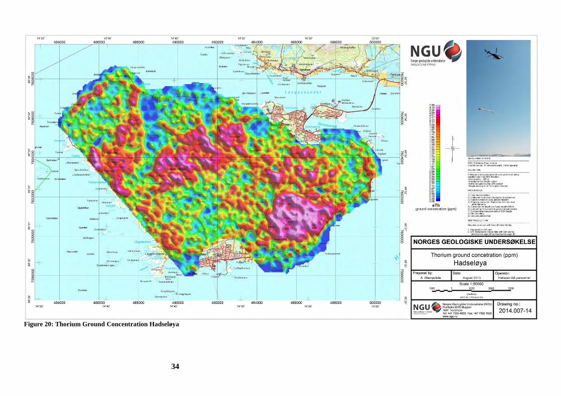
Hadseløya 2014.007-13 1:50000 Uranium ground concentration2014.007-14 1:50000 Thorium ground concentration2014.007-15 1:50000 Potassium ground concentration2014.007-16 1:50000 Radiometric Ternary Map

Downscaled images of the maps are shown on figures 7 to 22.

18

5. REFERENCES

Geosoft 2010: Montaj MAGMAP Filtering, 2D-Frequency Domain Processing of Potential FieldData, Extension for Oasis Montaj v 7.1, Geosoft Corporation

Geotech 1997: Hummingbird Electromagnetic System. User manual, Geotech Ltd, October 1997

Grasty, R.L., Holman, P.B. & Blanchard 1991: Transportable Calibration pads for ground andairborne Gamma-ray Spectrometers. Geological Survey of Canada, Paper 90-23: 62 pp.

IAEA 1991: Airborne Gamma-Ray Spectrometry Surveying, Technical Report No 323, Vienna,Austria, 97 pp.

IAEA 2003: Guidelines for radioelement mapping using gamma ray spectrometry data. IAEA-TECDOC-1363, Vienna, Austria, 173 pp.

Minty, B.R.S. 1997: The fundamentals of airborne gamma-ray spectrometry. AGSO Journal ofAustralian Geology and Geophysics, 17 (2): 39-50.

Minty, B.R.S., Luyendyk, A.P.J. and Brodie, R.C. 1997: Calibration and data processing forgamma-ray spectrometry. AGSO Journal of Australian Geology and Geophysics, 17(2): 51-62.

Naudy, H. and Dreyer, H. 1968: Non-linear filtering applied to aeromagnetic profiles. GeophysicalProspecting, 16(2): 171-178.

Rønning, J.S. 2013: NGUs helikoptermålinger. Plan for sikring og kontroll av datakvalitet. NGUIntern rapport 2013.001, (38 sider).

P1: Photo by Mari Nymoen, Telen Newspaper, Notodden

19

APPENDIX A1: FLOW CHART OF MAGNETIC PROCESSING

Meaning of parameters is described in the referenced literature.

Processing flow:

Quality control. Visual inspection of airborne data and manual spike removal Inspection of basemag data and removal of spikes Special Matlab convolution lowpass-filter for removal of 7.5 sec pendulum noise Import basemag data to Geosoft database Correction of data for diurnal variation and IGRF Splitting flight data by lines Gridding Micro-leveling USGS 2D-Frequency Domain filtering to remove high frequency noise and smooth data Grid knitting

APPENDIX A2: DESCRIPTION OF THE MATLAB CODE

The code is being used to filter the “pendulum effect” periodic noise on the magnetic data. The dataare filtered by calling a Matlab built-in convolution routine called “conv” that convolves the input datavector with a vector that has coefficients of Gaussian lowpass filter at a certain frequency (Freq.1).

If the differences between the input and the filtered data are above a predefined threshold, this part ofthe data is reprocessed be employing a less severe filter (Freq.2) on the input data. Again a thresholdis applied on the differences between the input and the filtered data and in this case if the differencesare above the threshold then the input data are retained for that part on the final filtered dataset.

These steps enable us to preserves the amplitudes of strong anomalies in the data, which will be lostotherwise by typical convolution or Fourier filtering. The cutoff frequency that were used wereFreq.1=0.04Hz and Freq.2=0.09Hz.

APPENDIX A3: FLOW CHART OF RADIOMETRY PROCESSING

Underlined processing stages are applied to the K, U, Th and TC windows.Meaning of parameters is described in the referenced literature.

Processing flow: Quality control Airborne and cosmic correction (IAEA, 2003)

Used parameters: (determined by high altitude calibration flights near Langoya in July 2013for the first system and at Frosta in May 2013 for the second system)

Channel Aircraft background counts Cosmic background counts

first system secondsystem

first system secondsystem

K 7.33 5.36 0.0617 0.0570

U 0.90 1.43 0.0454 0.0467

Th 0.89 0.00 0.0647 0.0643

Uup 0.39 0.70 0.0423 0.0448

Total counts 36.29 42.73 1.0379 1.0317

20

Radon correction using upward detector method (IAEA, 2003)

Used parameters (determined from survey data over water and land at Austvågøya-Hinnøya):

Coefficient Value Coefficient Valueau 0.34094 bu 0.0

aK 1.05146 bK 1.2984

aTh 0.06509 bTh 0.76857

aTC 20.4086 bTC 0.0

a1 0.0857759 a2 0.0173623

Stripping correction (IAEA, 2003)Used parameters (determined from measurements on calibrations pads at the NGU in May2013):

Coefficient first system second systema 0.049524 0.046856

b 0 0

c 0 0

α 0.29698 0.30346

β 0.47138 0.47993

γ 0.82905 0.82316

Height correction to a height of 60 mUsed parameters (determined by high altitude calibration flights at Frosta in Jan 2014):Attenuation factors in 1/m:

Channel first system second systemK -0.008884 -0.009523

U -0.006528 -0.006687

Th -0.006617 -0.007394

TC -0.007331 -0.00773

Converting counts at 60 m heights to element concentration on the groundUsed parameters (determined from measurements on calibrations pads at the NGU in May2013):Sensitivity (elements concentrations per count):

Channel first system second systemK (%/count) 0.007544793 0.007457884

U (ppm/count) 0.088909372 0.087729968

Th (ppm/count) 0.151433049 0.156658412

Microlevelling using Geosoft menu and smoothening by a convolution filtering

Microlevelling parameters valuesDe-corrugation cutoff wavelength (m) 2000

Cell size for gridding (m) 50

Naudy (1968) Filter length (m) 800

21

Figure 7: Total Magnetic Field anomaly Austvågøya-Hinnøya-Tjeldøya

22

Figure 8: Magnetic Vertical Gradient Austvågøya-Hinnøya-Tjeldøya

23

Figure 9: Magnetic Horizontal Gradient Austvågøya-Hinnøya-Tjeldøya

24

Figure 10: Magnetic Tilt Derivative Austvågøya-Hinnøya-Tjeldøya

25

Figure 11: Total Magnetic Field anomaly Hadseløya

26

Figure 12: Magnetic Vertical Gradient Hadseløya

27

Figure 13: Magnetic Horizontal Gradient Hadseløya

28

Figure 14: Magnetic Tilt Derivative Hadseløya

29

Figure 15: Uranium Ground Concentration Austvågøya-Hinnøya-Tjeldøya

30

Figure 16: Thorium Ground Concentration Austvågøya-Hinnøya-Tjeldøya

31

Figure 17: Potassium Ground Concentration Austvågøya-Hinnøya-Tjeldøya

32

Figure 18: Ternary Image of Radiation Concentrations Austvågøya-Hinnøya-Tjeldøya

33

Figure 19: Uranium Ground Concentration Hadseløya

34

Figure 20: Thorium Ground Concentration Hadseløya

35

Figure 21: Potassium Ground Concentration Hadseløya

36

Figure 22: Ternary Image of Radiation Concentrations Hadseløya

Geological Survey of NorwayPO Box 6315, Sluppen7491 Trondheim, Norway

Visitor addressLeiv Eirikssons vei 39, 7040 Trondheim

Tel (+ 47) 73 90 40 00Fax (+ 47) 73 92 16 20E-mail ngu@ngu.no Web www.ngu.no/en-gb/

Norges geologiske undersøkelsePostboks 6315, Sluppen7491 Trondheim, Norge

BesøksadresseLeiv Eirikssons vei 39, 7040 Trondheim

Telefon 73 90 40 00Telefax 73 92 16 20E-post ngu@ngu.no Nettside www.ngu.no

NGUNorges geologiske undersøkelseGeological Survey of Norway