nicot+scanlon es&t 12_si

Environmental Science & Technology:

Water Use for Shale-Gas Production in Texas, US

Jean- Philippe Nicot* and Bridget R. Scanlon

Bureau of Economic Geology, Jackson School of Geosciences, University of Texas at Austin

10100 Burnet Road, Building 130; Austin, TX, USA 78758

*corresponding author: [email protected] – 512 471-6246

Supporting Information:

Submitted March 1, 2012

26 numbered pages

14 figures

6 tables

mailto:[email protected]

Contents:

Units S1

Glossary S2

Conversion to English Units of Tables 1 and 2 S3

A -Transition to Horizontal Wells (historical water use) S4

B- Gas Production and Water Use Track One Another (historical water use) S5

C- Data Collection (historical water use) S6

D- Histograms of Water Use and Water Intensity (historical water use) S7

E- Auxiliary Water Use and Recycling (historical water use) S10

F- Prospectivity Factor (projected water use) S12

G- Distribution of Water use through Time (projected water use) S12

H- Assumption of No Refracking (projected water use) S13

I- Additional Plays—State-Level Water-Use Projections (projected water use) S14

J- Hydraulic-Fracturing Water Use Can be Significant at the County Level (proj. w.u.) S18

K- Water Efficiency of Energy Fuels S21

L- Application of the Methodology to other Plays S24

References S26

Tables:

Table S 1. Table 1 from main paper reproduced in English units S3

Table S 2.Table 2 from main paper reproduced in English units S3

Table S 3. Well count on water-use well data statistics S6

Table S 4. State-level 2008 water use in the mining S14

Table S 5. Projected county-level water use vs. planned water S19

Table S 6. Texas and overall water efficiency of various fuels (oil, gas, lignite) S22

Figures:

Figure S 1. Vertical vs. horizontal wells in the Barnett Shale play S4

Figure S 2. Cumulative gas production and water use; Barnett Shale play S5

Figure S 3. Histograms of water volume and intensity ( 2000–2010); Barnett Shale S7

Figure S 4. Histograms of water volume and intensity; Haynesville Shale S8

Figure S 5. Histograms of water volume and intensity; Eagle Ford S8

Figure S 6. Cumulative distribution function for water volume and intensity; all plays S9

Figure S 7. Locations of frac jobs (2005–2009) S15

Figure S 8. 2008 water use by mining category in Texas S15

Figure S 9. 2008 overall water use in Texas S16

Figure S 10. Summary of 2010–2060 projected net water use (mining industry) S16

Figure S 11. Summary of 2010–2060 projected net water use (oil and gas) S17

Figure S 12. Summary of 2010–2060 projected fracking net water use S17

Figure S 13. County projected fracking net water use vs. 2008 total water-use S20

Figure S 14. Net water-use patterns in various mining industries in Texas S23

Shale-gas water use, Nicot and Scanlon, Supporting Information

S1

Units:

There are numerous volume units even in the SI system, and, in addition, each engineering field

uses its customary units—barrel (bbl) and thousand cubic feet (Mcf) in the oil and gas industry,

million gallons (Mgal) and acre-feet (AF) in the water industry with the added complexity that

“m” or “M” often represents thousand and “MM” represents million in the oil and gas industry,

whereas “M” represent million or mega in the water industry. We used m3 and derivative units in

the main text with customary English unit equivalents that are also summarized below. Energy

units are also numerous, and we used SI units. SI units require the following prefixes: M, mega

for million, G, giga for billion, T, tera for thousand billion.

Mgal = mega gallon = million gallons; 1 Mgal = 3785 m3

Mm3 = mega m

3 = million m

3

Gm3 = giga m

3 = billion m

3 = 1 km

3

kAF = thousand acre-feet; 1 kAF = 1.23 Mm3

= 326 Mgal

GJ = giga joule = billion joules

MMBtu = million British thermal unit; 1 MMBtu = 1.055 GJ

Mcf = thousand cubic feet; 1 Mcf = 1×103 cf = 28.3 m

3

MMcf = million cubic feet; 1 MMcf = 1×106 cf = 0.0283 Mm

3

Bcf = billion cubic feet; 1 Bcf = 1×109 cf = 28.3 Mm

3

Tcf = Tera cubic feet; 1 Tcf = 1×1012

cf = 28.3 Gm3

Tm3 = Tera cubic meter; 1 Tm

3 = 1000 Gm

3 = 1×10

12 m

3


S2

Glossary

Core area: limited spatial area of a play with the highest productivity.

Depressurization: process by with water from an aquifer underlying an open-pit mine must be

withdrawn to decrease its pressure and avoid negative impacts

Enhanced Oil Recovery (EOR): process by which chemicals (CO2, solvents, polymers, etc.) are

injected into a reservoir in order to produce more oil; also called tertiary recovery. It is typically

undertaken after primary recovery (mostly pressure-driven) and waterflooding.

Estimated Ultimate Recovery (EUR): estimated amount of oil or gas potentially recoverable

from a play (play EUR) or a well (well EUR).

Hydraulic fracturing (sometimes spelled fracing or fracking): a stimulation method performed

in low-permeability formations consisting of creation of a connected fracture network by

increasing formation pressure (typically with high-rate water injection).

Completion: suite of operations to bring a well bore to production (including stimulation) after it

has been drilled.

Lateral: approximately horizontal leg of a so-called horizontal well bore. It generally stays in the

target formation and follows its dip.

Proppant: material added to frac fluid, whose role is to keep fractures open after pressure

subsides. Generally made of fit-for-purpose sand grains.

Proppant loading: proppant mass divided by water volume.

Stimulation: a treatment method to enhance production of a well (including hydraulic fracturing).

Waterflood / waterflooding: process by which water, generally saline water previously produced

from other wells but sometimes fresh water, is injected into a reservoir to produce more oil; also

called secondary recovery

Water use vs. net water use/water consumption: all projected water volumes related to fracking

and discussed in the main paper and the Supporting Information are consumptive, comparison to

uses outside of the upstream oil and gas industry are also mostly consumptive but not always.

Water-use intensity: amount of water used per unit length (water use divided by length of

vertical or lateral productive interval).

In the remainder of this supporting-material section we follow the general organization of the

paper. Heading numbering refers to citations in the main text.


S3

Conversion to English Units of Tables 1 and 2

Table S 1. Table 1 from main paper reproduced in English units

Formation Area

(mi2)

Use

(kAF)

Wells WUW

(Mgal)

WUI

(gal/ft)

Proj

(kAF)

Barnett 18,700 117 14,900 2.8 1000 853

TX-Haynesville 7,400 5.3 390 5.7 1120 425

Eagle Ford 20,400 14.6 1040 4.3 770 1,515

Other Shales 721

Tight Formations 725

Area: total area; Use: cumulative water use to 6/2011, Wells: number of wells to 6/2011 WUW: median water use

per horizontal well during the 2009–6/2011 period, WUI: median water-use intensity for horizontal wells during the

2009–6/2011 period, Proj: projected additional total water use by 2060. “Other shales” are mostly located in West

Texas whereas tight formations occur across the state.

Table S 2.Table 2 from main paper reproduced in English units

County 2008 Net Water Use Projected net Water Use

Name Population Area

(mi2)

Total

(kAF)

GW

(%)

SG

(kAF)

SG

(%)

Max

(kAF)

Max

(%)

Max

Year

Barnett

Denton1 637,400 952 98 13 2.7 2.8 1.7 1.7 2010

Johnson 155,200 727 29 45 8.5 29 3.3 11 2010

Parker 111,600 921 17 49 1.7 10 4.0 23 2010

Tarrant1 1,741,00 895 367 5 5.1 1.4 3.1 0.9 2010

Wise 58,500 927 12 42 2.2 19 4.6 40 2010

Eagle Ford

De Witt 20,200 909 6 86 2.3 35 2023

Dimmit 10,000 1,336 10 88 0.0 0.1 5.4 55 2015

Karnes 15,300 759 5 91 2.0 39 2018

La Salle 6,000 1,481 6 95 0.0 0.1 5.8 89 2019

Live Oak 12,100 1,074 7 66 0.8 12 2024

Webb2 238,300 3,394 45 3 0.0 0.0 2.4 5.2 2013

TX-Haynesville

Harrison 64,200 916 37 11 0.1 0.2 2.7 7.4 2017

Panola 23,300 820 8 37 0.0 0.5 2.4 30 2017

San Augustine 9,000 590 2 30 3.3 136 2017

Shelby 26,200 835 9 27 4.7 55 2017

Name: county name, Population: estimated 2008 population, Area: county area, Total: total net water use, GW:

estimated net groundwater use as a percentage of total net water use, SG: 2008 shale-gas net water use and

percentage of 2008 total net water use, Max: projected maximum shale-gas annual net water use and percentage of

2008 total net water use, Max Year: calendar year of projected maximum.

http://www.twdb.state.tx.us/wrpi/wus/2009est/2009County.xls 1 Includes City of Fort Worth and other communities relying primarily on imported surface water

2 Includes City of Laredo

3: Assumes that the water originates from the county in which it is used

http://www.twdb.state.tx.us/wrpi/wus/2009est/2009County.xls


S4

Historical Water Use

A -Transition to Horizontal Wells (historical water use)

Figure S 1 illustrates the transition from mostly vertical to mostly horizontal wells in the Barnett

Shale play. Elsewhere in Texas, some tight-gas plays still have mostly vertical wells, particularly

where operators target multiple horizons.

Figure S 1. Vertical vs. horizontal wells in the Barnett Shale play (incomplete data for 2009).


S5

B- Gas Production and Water Use Track One Another (historical water use)

There is a good match between cumulative gas production and fracking water use, illustrating the

fact that production needs to be constantly sustained by new wells (Figure S 2).

Figure S 2. Cumulative gas production and water use track each other ll in the development /

extension phase of the Barnett Shale play.


S6

C- Data Collection (historical water use)

Although the list of all wells drilled and hydraulically fractured is easily accessible, the amount

of water used is sometimes not readily available for a fraction of the wells. Table S 3 gives the

breakdown in terms of processing raw data downloaded from the vendor database (IHS). Well-

completion data from the Barnett Shale are mostly complete, whereas well-completion data for

the Eagle Ford and Haynesville Shales are less complete, requiring assumptions to access water

use through use of proppant loading and length of laterals.

Wells with water use ≤380 m3 (<0.1 Mgal) were omitted from analysis. This threshold is

somewhat arbitrary but convenient and was used to distinguish current high-volume frac jobs

from simple well stimulation by traditional fracking and acid jobs. They represented two

different populations as shown by bimodal or multimodal histograms of water use per well. In

2010, out of all the plays in Texas with some fracking, 3841 wells underwent fracking with a

water volume >0.1 Mgal and frequently >>0.1 Mgal (Table 8 in Nicot et al.),1 3809 wells, the

vast majority of which is vertical, were stimulated with water volume <0.1 Mgal and often <<0.1

Mgal, and 2712 other wells were drilled but neither fracked or stimulated. A quick analysis

shows that the wells with mild stimulation do not contribute much to the overall water use: 3809

wells × 0.1 Mgal/well / 0.325851 AF/Mgal = 1170 AF or 1.2 kAF (1.4 Mm3) at most and

actually much less because 0.1 Mgal is the upper bound. This value is to be compared to the

>35kAF (45 Mm3) estimated to be used for high-volume fracking during the same time (Table S

4).

Table S 3. Well count on water-use well data statistics to estimate historical fracking water use.

Barnett Haynesville

(TX+LA)

Eagle Ford

Wells % of Total Wells % of Total Wells % of Total

Water use and proppant use 3374 97 394 33 279 59

Estimated from proppant use 70 2 150 12 147 31

Estimated from lateral length 43 1 629 52 46 10

Assigned average water use 2 0 32 3 2 0

Total 3489 100 1,205 100 474 100

Period from 1/1/2009 to 12/31/2010


S7

D- Histograms of Water Use and Water Intensity (historical water use)

The following histograms show distributions of frac-water volume and water intensity in the

Barnett (Figure S 3), Haynesville (Figure S 4), and Eagle Ford (Figure S 5) shales for selected

years. Figure S 6 reproduces the same information and compares plays. The information was

used to estimate projected water use. A detailed examination of water intensity through the years

suggests that the industry is becoming more efficient and uses progressively less water per unit

length of lateral.

Figure S 3. Histograms of frac water volume for vertical wells, horizontal wells, and water

intensity for the 2000–2010 period in the Barnett Shale play (1000 m3 = 0.26 Mgal; 10 m

3/m =

805 gal/ft).


S8

Figure S 4. Histograms of horizontal well frac water volume and water intensity in the

Haynesville Shale play (Texas and Louisiana) (1000 m3 = 0.26 Mgal; 10 m

3/m = 805 gal/ft).

Figure S 5. Histograms of horizontal well frac water volume and water intensity in the Eagle

Ford Shale play (1000 m3 = 0.26 Mgal; 10 m

3/m = 805 gal/ft).


S9

Figure S 6. Data-based cumulative distribution function for horizontal well frac water volume

and water intensity in the Barnett, Haynesville (TX+LA), and Eagle Ford Shale plays (1000 m3 =

0.26 Mgal; 10 m3/m = 805 gal/ft)


S10

E- Auxiliary Water Use and Recycling (historical water use)

Auxiliary water use related to drilling and proppant mining (sand mining for proppant production)

can be counted toward shale-gas development, in addition to fracking.

Drilling water use is variable depending on the play and technological choices of the operator.

Well drilling requires a fluid carrier to remove the cuttings and dissipate heat created at the drill

bit. The fluid also keeps formation-water pressure in check. Broadly, three types of fluids are

used: (1) air, air mixtures, and foams (2) water-based muds, and (3) oil-based muds. Although

the most common method involves water-based muds, shale operators tend to rely on the other

methods more than the other operators. The amount of water used for drilling varies across plays

and, within a play, is operator-dependent. It follows that, water use for drilling shale-play wells

is only loosely correlated with depth. Nicot et al.1 proposed several approaches and suggested an

average of 500 m3 (0.13 Mgal) per well for the ~10,000 wells (40% of which were hydraulically

fractured, and 16% of which were shale-gas wells) drilled in Texas in 2008. DOE2 (p. 64) put

forward an estimate of 1500 and 3700 m3 (400,000 and 1,000,000 gal) to drill a well in the

Barnett and Haynesville shales, respectively. Some operators have released specific information

about drilling water use, but the amount varies across plays and with different operators.3 In this

rapidly evolving technological field, information quickly become outdated; e.g., Chesapeake4

listed values of 950 m3/well (250,000 gal, Barnett), 2300 m

3/well (600,000 gal, Haynesville), and

500 m3/well (125,000 gal, Eagle Ford); that is, 6.2%, 10.8%, and 2.0% of combined drilling and

fracking water use, respectively—lower numbers than those reported by DOE.2

Sand for proppant (one use of industrial sand) is often mined from natural sand deposits and

requires more water than typical aggregate plants because of the grain-size sorting involved,

despite intense water recycling at these facilities. Nicot et al.1 (p.161) estimated industrial

sand/proppant net water use in Texas to be ~2.5 m3 of water per metric ton of proppant (~600

gal/short ton or 0.3 gal/lb). Combining this statistic with an average proppant loading of 72 kg of

proppant/m3 of frac fluid (0.6 lb/gal) yields a value of 0.18 m

3 of water for proppant production

per m3 of frac fluid (0.18 gal of water for proppant production per gal of frac fluid).

Overall, these two additional water uses (drilling and sand mining) amount to an additional

~25% of water use relative to water used solely for fracking. Note that some deep plays such as

the Haynesville Shale use man-made ceramics proppant and that some of the proppant can be

imported from out of state.


S11

Recycling and reuse of fracking fluids are possible only on the fraction flowing back to the

wellhead. This fraction is variable and a function of the play, location within the play, and of the

fracking operational details. Operational issues also render the use of flowback/produced water

feasible only early in the history of the well (weeks). It follows that the usable water volume is

lower and sometimes much lower than the total water volume that flows back. Mantell3 reported

that 10 days after fracking, only 16% and 5% of the frac fluid had been recovered in the Barnett

and Haynesville shales, respectively, although ultimately about 3 to 1 times the injected volume

will be produced from the same plays during the life of the wells in these plays. Another

important parameter is water quality; in some cases treatment of flowback water is not

economical, and the best approach to dispose of flowback water is deep well injection. Nicot et

al.1 estimated that, in the past few years, recycling water use was within the 5–10% range in the

Barnett and ~0% in the Tx-Haynesville shales. No information was collected for the Eagle Ford

Shale. Ultimately, the level of reuse and recycling may revolve around economics relative to

other options such as deep well injection, which is commonly used in Texas.


S12

Projected Water Use

F- Prospectivity Factor (projected water use)

A prospectivity factor is assigned to each county (or portion of county within the play footprint).

It varies in the 0-1 range. A factor close to 1 is typically assigned to counties in the core area

decreasing to 0 at the edge of the gas shale footprint. The prospectivity factor is one of the least

known parameters and it gives a competitive edge to the companies with a good knowledge of it.

Prospectivity factor includes assessment of characteristics that are readily available such as shale

depth and thickness but also elements or features such as amount and type of organic matter,

thermal maturity, burial history, microporosity, and fracture spacing and orientation.

Prospectivity factor also includes impacts of cultural factors such as urban or rural environment.

Although not an issue in Texas, it could also account for difficulties with local topography. By

definition the value of the prospectivity factor is subjective but based on limited objective

information on the elements listed above. The county-level estimates used in this work relied on

educated estimates resulting from discussions with expert geologists.

G- Distribution of Water use through Time (projected water use)

Temporal distribution of water use may be as complex as allowed by data availability. A very

simple methodology would consist is estimating the life of the play (for example, 20 or 40 years)

and assuming a constant rate of drilling/fracking through time and space. In this paper,

drilling/fracking rates are considered variable through time and are characterized by a start year,

a peak year, and an end year at the county level. The start year is either in the past if drilling is

already active in the county or in the future if no well or only a few wells have been drilled. The

start year is assigned as a function of the prospectivity, that is, a more prospective county will

have an earlier start year than a less prospective county. Peak year is approximately 10 years

after the start year and is followed by a long tail of approximately 20 to 50 years until high-

volume fracking stops in the county. Those values were derived from a more detailed work done

on the Barnett Shale and assumed valid for the state as a whole.1 The number of wells fracked in

the peak year is a function of the prospectivity of the county. The four parameters for each

county (start year, peak year, end year, and number of wells fracked at peak year) are then

iterated until (1) the overall number of fracked wells is consistent with the number of drilling rigs

available in the play (in general 50 to 250 rigs) and the “spud-to-spud” time interval (time


S13

between time zero of successive wells, 2 to 5 weeks depending on depth, play and operator) and

(2) the overall peak year of the play is somewhat consistent with the projected evaluation of the

plays as published in the public domain by oil and gas companies, think tanks, and other

consultancies (well and play EURs, IPs).1

H- Assumption of No Refracking (projected water use)

This study assumes that all possible refracking has already been done and that there will be no

need to refrac newer wells. Access to refrac information in Texas is not as straightforward as that

for initial completion. How much refracking of wells already fracked is occurring or will occur is

unclear, and the information is conflicting. Vincent5 did a systematic study of refracking from

the beginning of hydraulic fracturing and concluded that refracking works in some areas and not

in other areas (note that successful or unsuccessful fracs use the same amount of water). Cases

where refracking works are well documented in the literature and cases where refracking does

not work are not documented as often. However, discussions with operators suggest that very

little refracking of recent or future wells will occur. Refracking activities so far have been

restricted to wells completed early in the development of the slick-water fracking technology and,

thus, may be more common for vertical wells. Potapenko et al.6, evaluating Barnett

recompletions, found that despite great success with refracking of vertical wells, little success

has come from refracking of horizontal wells. Gel fracs performed early in the history of the play

may have damaged the formation, and new water fracs have restored its full potential.7 Sinha and

Ramakrishnan8 suggested that 15-20% of the Barnett Shale horizontal wells have some attributes

that make them suitable candidates for refracking. Eventually, the impact of refracking will be a

function of the future price of natural gas, with a higher price likely leading to more refracs.


S14

I- Additional Plays—State-Level Water-Use Projections (projected water use)

In addition to the three plays considered in this study (Barnett, Haynesville, and Eagle Ford

shales), several others have growing potential, as well as many more tight plays. Tight plays are

whole or portions of conventional reservoirs with very low permeability (<1 md) (Figure S 7).

Tight gas plays represented the bulk of fracking before development of shale gas. Wells in these

tight plays tend to be vertical; however, many are horizontal. Table S 4 shows the water-use

breakdown by mining category in Texas for 2008, the last year with a complete data set. Figure S

8 displays the same information in a column chart. Figure S 9 illustrates the fact that mining

(including fracking) water use (mostly consumptive) is a small fraction of total water use in

Texas (mostly consumptive). The projections assume that extrapolation from current trends is

appropriate. Unpredictable events, by their nature, are not included, and the multiplicity of

potential scenarios quickly becomes unmanageable: what year does it begin, how rapidly does it

develop, is it permanent or transient, what is the magnitude of the impact, etc.? Including

uncertainty in changes in water-use projections is extremely difficult; therefore, our approach

focused on a single best estimate. Figure S 10, Figure S 11, and Figure S 12 illustrate water use

(mostly consumptive) through time for the entire mining industry, oil and gas sectors, and

fracking only, respectively.

Table S 4. State-level 2008 water use, mostly consumptive, in the mining industry (not including

any postmining processing water use).1

Hydraulic

Fracturing

EOR Drilling Coal Crushed

Stone

Sand &

Gravel

Industrial

Sands

Others Total

Mm3 44.7 16.0 9.9 24.5 65.7 22.6 12.0 1.6 197.0

kAF 36.2 13.0 8.0 19.9 53.3 18.3 9.7 1.3 159.7

Mgal 11.8×103 4.2×10

3 2.6×10

3 6.5×10

3 17.4×10

3 6.0×10

3 3.2×10

3 0.4×10

3 52.0×10

3


S15

Figure S 7. Map showing locations of all frac jobs in the 2005–2009 time span in Texas.

Approximately 23,500 wells are shown.

Figure S 8. Summary of 2008 water use by mining category in Texas (all sources). All

categories are consumptive except some coal operations withdrawing water from aquifers (that is,

consumptive for the aquifers) and redirecting them to surface water bodies.


S16

Figure S 9. Summary of 2008 overall water use in Texas. Irrigation, livestock, steam electric,

and mining are overall consumptive. Water use for municipal and manufacturing is only partly

consumptive because some of the water is returned to surface water bodies (lakes, rivers) and

could be used again.

Figure S 10. Summary of 2010–2060 projected net water use in the mining industry segment

(some coal water use can be considered as non- consumptive).


S17

Figure S 11. Summary of 2010–2060 projected net water use in the oil and gas segment.

Figure S 12. Summary of 2010–2060 projected fracking shale-gas and tight-formation net water

use.


S18

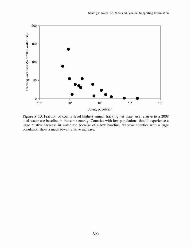
J- Hydraulic-Fracturing Water Use Can be Significant at the County Level (projected water

use)

Fracking net water use does not represent a large fraction of total water use (mostly consumptive)

at the state level; however, it can represent a significant fraction at the county level, particularly

rural counties with low populations, whose main water source is aquifers (Figure S 13). However,

projected fracking demand (that can be met from a strictly groundwater-availability standpoint)

is not necessarily within the projected net water use agreed upon by local governing bodies, i.e.

groundwater conservation districts. At the county level, projected fracking net water use is

sometimes larger than projected pumping for all other uses (Table S 5), as illustrated by the

following example chosen in the Eagle Ford Shale, where most frac water is derived from

groundwater. Karnes County is projected to have a maximum annual fracking net water use of

2.5 Mm3 (2.0 kAF) and an average fracking net water use of 1.3 Mm

3/yr (1.1 kAF/yr) in 2010–

2060. However, local water governmental entities have projected average annual water use for

all usages over the 2010–2060 period (not including fracking) of 2.3 Mm3/yr (1.9 kAF/yr). This

value was agreed upon by various entities to protect long-term use of the aquifers. Including

(exempted) fracking net water use will increase water use by 56% beyond agreed-upon water use.

That is, averaged over the 2010–2060 period, several counties may need to provide more water

for fracking relative to all other planned water uses.


S19

Table S 5. Projected county-level water use vs. planned water use through desired future

conditions.

2008 Water Use Projected Water Use

County Total

(Mm3)

GW

(%)

SG

(Mm3)

SG

(%)

Max frac

(Mm3)

Max frac

(%)

Mean DFC

(Mm3/yr)

1

Mean frac

(Mm3/yr)

Mean frac

(%)

De Witt 7.9 86 2.8 35.4 18.02 1.5 8.3

Dimmit 12.2 88 0.0 0.1% 6.7 55.1 2.73 3.5 130

Karnes 6.2 91 2.5 39.4 2.33 1.3 56.5

La Salle 8.0 95 0.0 0.1% 7.1 89.2 5.33 3.5 66.0

Live Oak 8.4 66 1.0 12.3 14.24 0.5 3,5

Webb 56.0 3 0.0 0.0% 2.9 5.2 1.13 1.5 136

English Units

County Total

(kAF)

GW

(%)

SG

(kAF)

SG

(%)

Max frac

(kAF)

Max frac

(%)

Mean DFC

(kAF /yr)1

Mean frac

(kAF /yr)

Mean frac

(%)

De Witt 6.4 86 2.3 35.4 14.62 1.2 8.3

Dimmit 9.9 88 0.0 0.1% 5.4 55.1 2.23 2.8 130

Karnes 5.1 91 2.0 39.4 1.93 1.1 56.5

La Salle 6.5 95 0.0 0.1% 5.8 89.2 4.33 2.8 66.0

Live Oak 6.8 66 0.8 12.3 11.54 0.4 3,5

Webb 45.4 3 0.0 0.0% 2.4 5.2 0.93 1.2 136

Total: total water use, GW: estimated groundwater-use percentage of total, SG: shale-gas water use and

percentage of total, Max frac: projected maximum shale-gas annual net water use and percentage of 2008

total water use, Mean DFC: mean desired future condition (DFC) pumping 2010–2060, Mean Frac:

projected mean annual fracking net water use 2010–2060 and percentage of DFC pumping. 1De Witt and Live Oak Counties are mostly over the Gulf Coast aquifers.

2TWDB, 2011, GAM Run 10-008 Addendum by S. C. Wade; Groundwater Management Area #15 has chosen

pumping level corresponding to an average drawdown of 12 ft in the Gulf Coast aquifers over the 2010–2060

period across the whole GMA #15 area;

http://www.twdb.state.tx.us/GwRD/GMA/gmahome.htm 3TWDB, 2010, GAM Run 09-034 by S. C. Wade and M. Jigmond; Scenario 4 has been retained by Groundwater

Management Area #13 to establish DFCs corresponding to an average drawdown of 23 ft in the Carrizo aquifer

over the 2010–2060 period across the whole GMA #13 area;

http://www.twdb.state.tx.us/GwRD/GMA/gmahome.htm 4TWDB, 2011, GAM Run 09-008 by W. R. Hutchinson; Scenario 10 has been chosen by Groundwater Management

Area #16 to establish DFCs corresponding to an average drawdown of 94 ft in the Gulf Coast aquifers over the

2010–2060 period across the whole GMA #16 area;

http://www.twdb.state.tx.us/GwRD/GMA/gmahome.htm





S20

Figure S 13. Fraction of county-level highest annual fracking net water use relative to a 2008

total-water-use baseline in the same county. Counties with low populations should experience a

large relative increase in water use because of a low baseline, whereas counties with a large

population show a much lower relative increase.


S21

K- Water Efficiency of Energy Fuels

Water efficiency for energy fuels can be computed in multiple ways all based on the ratio of net

water use in a given period over fuel production (or its energy content) over the same period.

However, depending on the water use and fuel-production pattern (Figure S 14), the ratio for a

given fuel may vary. The geographic base used to compute water efficiency and varying water

efficiencies through time complicates the analysis. For example, fresh water use for waterfloods

(process by which water, generally saline water previously produced from other wells but

sometimes fresh water, is injected into a reservoir to produce more oil) has been decreasing

constantly for several decades, although the fraction of oil extracted through secondary and

tertiary recovery has increased at the same time. Gleick9 concluded that water efficiency for

waterflood oil was >600 liter per gigajoule (L/GJ) (Table S 6). Nicot et al.1 reported a somewhat

lower value of 115 L/GJ in West Texas in 1994. That same value applied to the entire state for

the same year at a time with large oil primary production would yield a low value of 5.8 L/GJ.

Instantaneous water efficiency as computed in 2008 for oil was 13 L/GJ (8.6 L/GJ when applied

to the whole state). Applying fracking net water use to gas production in the entire state in 2008

yields a water efficiency of 4.6 L/GJ. Water efficiency depends also on the granularity of the

system, with oil and gas relative to coal representing opposite extremes. Including

depressurization (process by with water from an aquifer underlying an open-pit mine must be

withdrawn to decrease its pressure and avoid negative impacts) or not affects water efficiency for

lignite by a factor of ~8. A mine requiring large-scale depressurization pumping recently closed

down1 and with it, efficiency numbers would have been less favorable.


S22

Table S 6. Texas and overall water efficiency of various fuels (oil, gas, lignite).

Gleick9 (1994)

DOE10

(2006)

Mantell11

(2009)

(Liter/GJoule)

Nicot et al.1

(Liter/GJoule)

Oil 3-8 [glk]

Waterflood – CO2-EOR 600-640 [glk]

West Texas, 19941 115

Applied to whole state, 1994 (mixed)2 5.8

West Texas, 20023 21.6

Applied to whole state, 2002 (mixed) 14.0

West Texas, 20081 13.0

Applied to whole state, 2008 (mixed) 8.6

Oil refining 25-65[glk]

Gas ~0 [glk]

Barnett Shale4 4.8 [mtl]

Haynesville Shale (TX and LA)4 2.3 [mtl]

Texas shale gas (2010)4 8.3

Including drilling and proppant mining 10.4

All Texas gas (2010)5 4.6

Gas processing6 6 [glk]

Coal (no washing) 3.6-21.6 [doe]

Coal surface mining (no reclamation) 2 [glk]

Coal surface mining (reclamation) 5 [glk]

Lignite (consumption only) ~8.3-16.6

Lignite (depressurization included) ~63-126

Uranium (in situ recovery, no reclamation) ~6.1

Uranium open-pit mining 20 [doe] [glk]

Postmining processing 26-30 [doe] [glk]

The following conversion factors were used: 1 bbl oil ~ 5.9 MMBtu; 1 Mcf gas ~ 1 MMBtu; 1 ton lignite ~ 9-18

MMBtu; 1 lb U ~170 MMBtu; 1 MMBtu = 1.055 GJ; 1Only counties with significant waterflood

2Texas oil production was greater in 1994 (542 million barrels) than in 2002 (365) or 2008 (353)

3All counties, assuming that ~two-thirds of the oil was produced through secondary or tertiary recovery (Nicot et

al.,1, p.114)

4Mantell

11 estimates include all production to EUR (“ultimate water efficiency”), whereas figures extracted from

Nicot et al.1 include only gas produced during the year for which water use was computed (“instantaneous water

efficiency”). Drilling is also included. Mantell11

also included 1.8 gal/MMBtu for the Fayetteville Shale in

Arkansas and 1.05 gal/MMBtu for the Marcellus Shale in Pennsylvania. 52010 water-use fracking for gas wells was 35.2 Mm

3 (28.5 kAF), 2010 total gas production in Texas was 205 Gm

3

(7.25 Tcf) (http://www.rrc.state.tx.us/data/petrofacts/July2011.pdf), with 2010 shale-gas production accounting for

about one-third of it. 6Not all gas produced requires processing.

http://www.rrc.state.tx.us/data/petrofacts/July2011.pdf


S23

Production

Production

Production

Time

Am

ount

Shale gas

Oil

Coal and uranium

Am

ount

Am

ount

Water use

Water use

Water use

Figure S 14. Illustration of net water-use (water consumption) patterns in various mining

industries in Texas. Time frame varies from years to decades. The relative size of the production

and water-use curves and the relative size of the three water use curves are only indicative and

should not be quantitatively compared with one another. Fracking consumes all water upfront

and oil/gas production slowly declines. In the conventional oil production case, the initial

amount of fresh water consumed during waterflood and EOR decreases through time as the water

produced from the production well is reinjected and as oil production reaches a relative plateau.

Typically, both injection and production stop within the same year. Water consumption for

coal/lignite production is very variable in Texas, from almost non-existent to large. The figure

represents a case with sustained depressurization throughout the life of the facility and the

subsequent water needed for reclamation (which lags production by a few years). Uranium

mining follows a similar pattern but for different reasons and with a much smaller absolute water

volume. Most uranium is produced through in-situ recovery in which chemical are injected with

water to leach the uranium from the rock. More water is produced than injected to maintain a

negative pressure and avoid contaminant excursion. A cleaning and reclamation period follows.


S24

L- Application of the Methodology to Other Plays

The methodology formulated in this study can be divided into 2 major steps: (1) obtain and

process historical data and assess trends in key parameters, and (2) apply a prospectivity factor to

obtain an overall water use for the play and then distribute it through time. It is mostly applicable

to plays in which horizontal wells are the production method of choice.

The first step is accomplished through data mining of the IHS or another database to obtain the

water intensity I (m3 or gal of water per m or ft of lateral) and its trend through time. Mapping of

the boreholes in the areas the most densely drilled allows for an estimate of the lateral spacing d.

If the play is new or if the researcher lacks access to databases, ranges of water intensity and of

lateral spacing provided in this work can be used as an initial estimate. Now, imagining that

some domain of area D is entirely drilled with, in essence, parallel laterals covering the whole

domain end to end with a spacing of d, the uncorrected water use Wu for the domain of area D

would be: Wu = D/d×I.

In a second step, the prospectivity factor p is applied to the domain of area D to yield a corrected

water use factor Wc: Wc = p×Wu = p×D/d×I. Details on the prospectivity factor are given in

Section F. If the play has already been active, the p factors can be varied between the different

domains making up the play (counties in this study), with values close to 1 in the core area to

values close to 0 at the edge of the play (keeping in mind that the core is not necessarily at the

center of the play). If no information is available, we suggest a prospectivity factor value taken in

the 0.2-0.4 range. The water use Wc represents the cumulative amount of water used during the

life of the play.

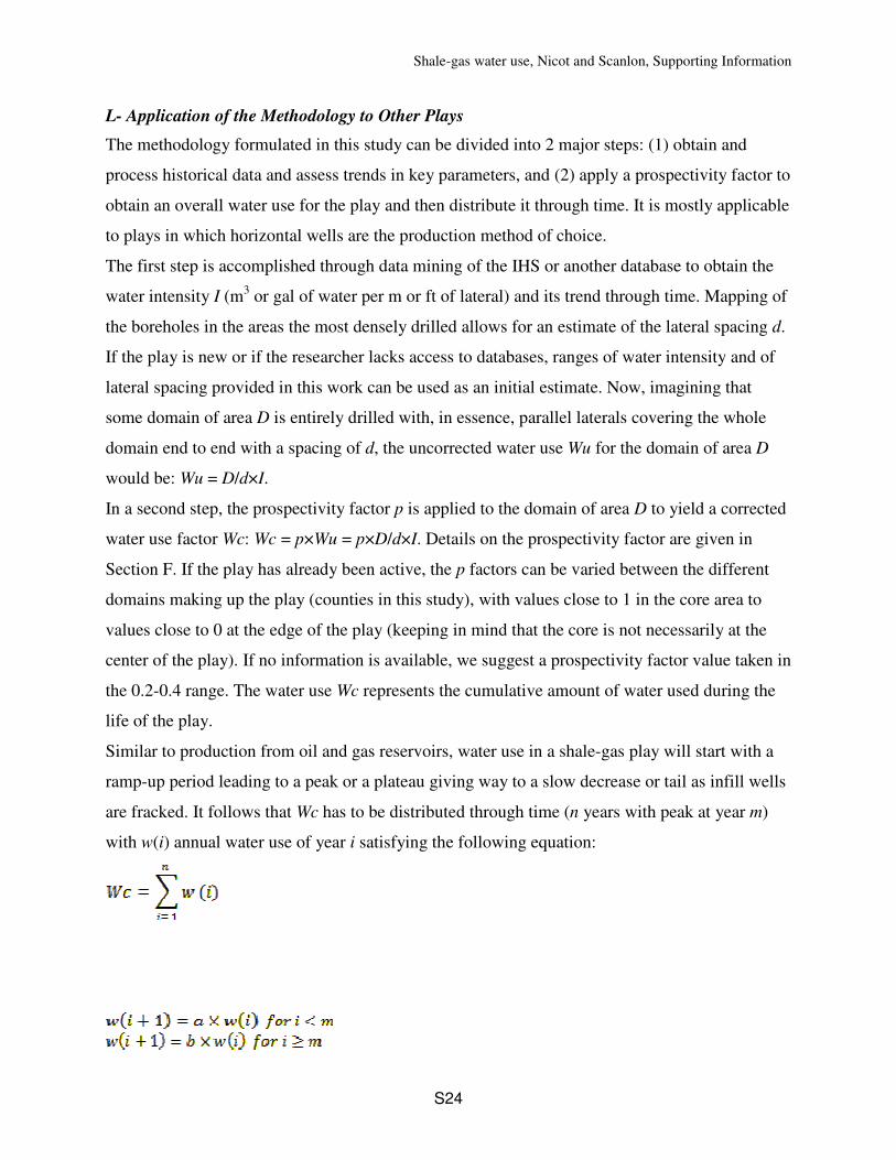
Similar to production from oil and gas reservoirs, water use in a shale-gas play will start with a

ramp-up period leading to a peak or a plateau giving way to a slow decrease or tail as infill wells

are fracked. It follows that Wc has to be distributed through time (n years with peak at year m)

with w(i) annual water use of year i satisfying the following equation:


S25

The constraints simply mean that the time distribution of water use has a triangular shape with

ascending and descending straight lines converging at year m. if no other information is

available, values for parameters n and m can be extracted from Figure 4 of the main paper. It

shows estimated time distribution of projected water use for the three main shale-gas plays in

Texas. Note that this approach assumes no refracking (Section H). Water use values w(i) for

early time (i≤10) have to be consistent with the average time to drill a well and the anticipated

rig count (Section G) in the play, itself consistent with the rig count of the multi-state region

competing for rigs. Finally, recycling/reuse (Section E) is added to the estimated water use

through a time varying factor r(i)≤1. This study assumes that r varies from 1 when no

recycling/reuse occurs to 0.8 for the Barnett and Eagle Ford shale plays in 2060 (that is, 20% of

the water injected is recycled/reused). The net water use for year i is r(i)×w(i) and the total net

water use Wnet in the domain D is:

The net water use Wnet can then be compared to local surface water and groundwater use. All

final projection results presented in this work are net water use (Wnet).


S26

References

1. Nicot, J.-P.; Hebel, A.; Ritter, S.; Walden, S.; Baier, R.; Galusky, P.; Beach, J. A.; Kyle,

R.; Symank, L.; Breton, C. Current and Projected Water Use in the Texas Mining and Oil and

Gas Industry. Bureau of Economic Geology. Report prepared for Texas Water Development

Board 2011, 357 pp.

2. DOE Modern Shale Gas Development in the United States: a Primer. Report prepared by

Ground Water Protection Council, Oklahoma City and ALL Consulting, Oklahoma City, for

Office of Fossil Energy and NETL, U.S. Department of Energy, April 2009, 96 pp.

3. Mantell, M. E. Deep shale natural gas and water use, part two: abundant, affordable,

and still water efficient. Presentation at Ground Water Protection Committee 2010 Annual

Forum “Water and Energy in Changing Climate” September 28, 2010.

4. Chesapeake Information sheets from corporate website,

http://www.chk.com/Environment/Water/Pages/information.aspx 2011.

5. Vincent, M. C. Refracs—Why do they work, and why do they fail in 100 published field

studies? Society of Petroleum Engineers Paper #134330 2010.

6. Potapenko, D. I.; Tinkham, S. K.; Lecerf, B.; Fredd, C. N.; Samuelson, M. L.; Gillard, M.

R.; LeCalvez, J. H.; Daniels, J. L. Barnett Shale refracture stimulations using a novel diversion

technique. Society of Petroleum Engineers Paper #119636 2009.

7. King, G. W. Thirty years of gas shale fracturing: what have we learned. Society of

Petroleum Engineers Paper #133456 2010.

8. Sinha, S.; Ramakrishnan, H., A novel screening method for selection of horizontal

refracturing candidates in shale gas reservoirs. Society of Petroleum Engineers Paper #144032

2011.

9. Gleick, P. H., Water and energy. Annual Rev. Energy Environ. 1994, 19, 267-299.

10. DOE Energy Demands on Water Resources. Department of Energy Report to Congress

on the Interdependency of Energy and Water; Department of Energy: Washington, DC 2006, 80

pp.

11. Mantell, M. E. Deep Shale Natural Gas: Abundant, Affordable, and Surprisingly Water

Efficient. Water/Energy Sustainability Symposium: Groundwater Protection Council (GWPC)

Annual Forum, Salt Lake City, Utah 2009, 15 pp.

http://www.chk.com/Environment/Water/Pages/information.aspx

nicot+scanlon es&t 12_si

Presentations & Public Speaking