NIKHEF/2013-010

Life at the Interface of Particle Physics and String Theory∗

A N Schellekens

Nikhef, 1098XG Amsterdam (The Netherlands)IMAPP, 6500 GL Nijmegen (The Netherlands)IFF-CSIC, 28006 Madrid (Spain)

If the results of the first LHC run are not betraying us, many decades of particle physicsare culminating in a complete and consistent theory for all non-gravitational physics:the Standard Model. But despite this monumental achievement there is a clear senseof disappointment: many questions remain unanswered. Remarkably, most unansweredquestions could just be environmental, and disturbingly (to some) the existence of lifemay depend on that environment. Meanwhile there has been increasing evidence thatthe seemingly ideal candidate for answering these questions, String Theory, gives ananswer few people initially expected: a huge “landscape” of possibilities, that can berealized in a multiverse and populated by eternal inflation. At the interface of “bottom-up” and “top-down” physics, a discussion of anthropic arguments becomes unavoidable.We review developments in this area, focusing especially on the last decade.

CONTENTS

I. Introduction 2

II. The Standard Model 5

III. Anthropic Landscapes 10A. What Can Be Varied? 11B. The Anthropocentric Trap 12

1. Humans are irrelevant 122. Overdesign and Exaggerated Claims 123. Necessary Ingredients 134. Other Potentially Habitable Universes 13

C. Is Life Generic in QFT? 15D. Levels of Anthropic Reasoning 17E. First Signs of a Landscape? 18

1. Particle Physics 192. Cosmology 193. The Cosmological Constant 21

F. Possible Landscapes 241. Fundamental Theories 242. The role of gravity 253. Other Landscapes? 254. Predictive Landscapes 265. Catastrophic Landscapes 276. Expectations and implications 28

IV. String Theory 28A. Generalities 28B. Modular invariance 29

1. Finiteness and Space-time Supersymmetry 302. Ten-dimensional Strings 30

C. D-branes, p-forms and Fluxes 30D. Dualities, M-theory and F-theory 31E. The Bousso-Polchinski Mechanism 32F. Four-Dimensional Strings and Compactifications 32

1. Landscape Studies versus Model Building 332. General Features 333. Calabi-Yau Compactifications 344. Orbifold Compactifications 355. The Beginning of the End of Uniqueness 35

∗ Extended version; see also www.nikhef.nl/∼t58/Landscape

6. Free Field Theory Constructions 357. Early attempts at vacuum counting. 368. Meromorphic CFTs. 379. Gepner Models. 37

10. New Directions in Heterotic strings 3811. Orientifolds and Intersecting Branes 3912. Decoupling Limits 41

G. Non-supersymmetric strings 42H. The String Theory Landscape 43

1. Existence of de Sitter Vacua 432. Counting and Distributions 453. Is there a String Theory Landscape? 46

V. The Standard Model in the Landscape 46A. The Gauge Sector 46

1. Gauge Group and Family Structure 462. The Number of Families 473. Grand Unification in String Theory 484. Coupling Constant Unification 515. The Fine-structure Constant 53

B. Masses and Mixings 541. Anthropic Limits on Light Quark Masses 542. The Top Quark Mass 613. Charged Lepton Masses 624. Masses and Mixings in the Landscape 625. Landscape vs. Symmetries 636. Neutrinos 64

C. The Scales of the Standard Model 661. Changing the Overall Scale 672. The Weak Scale 68

D. Axions 73E. Variations in Constants of Nature 75

VI. Eternal Inflation 77A. Tunneling 77B. The Measure Problem. 77

1. The Dominant Vacuum 782. Local and Global Measures 79

C. Paradoxes 791. The Youngness Problem 792. Boltzmann Brains 80

VII. The Cosmological Constant in the String Landscape 81

VIII. Conclusions 82

2

Acknowledgments 83

References 84

I. INTRODUCTION

In popular accounts, our universe is usually describedas unimaginably huge. Indeed, during the last centurieswe have seen our horizon expand many orders of magni-tude beyond any scale humans can relate to.

But the earliest light we can see has traveled a mere13.8 billion years, just about three times the age of ourplanet. We might be able to look a little bit further thanthat using intermediaries other than light, but soon weinevitably reach a horizon beyond which we cannot see.

We cannot rule out the possibility that beyond thathorizon there is just more of the same, or even nothing atall, but widely accepted theories suggest something else.In the theory of inflation, our universe emerged from apiece of a larger “space” that expanded by at least sixtye-folds. Furthermore, in most theories of inflation ouruniverse is not a “one-off” event. It is much more plau-sible that the mechanism that gave rise to our universewas repeated a huge, even infinite, number of times. Ouruniverse could just be an insignificant bubble in a gi-gantic cosmological ensemble, a “multiverse”. There areseveral classes of ideas that lead to such a picture, butthere is no need to be specific here. The main point isthat other universes than our own may exist, at least ina mathematical sense. The universe we see is really justour universe. Well, not just ours, presumably.

The existence of a multiverse may sound like specula-tion, but one may as well ask how we can possibly becertain that this is not true. Opponents and advocatesof the multiverse idea are both limited by the same hori-zon. On whom rests the burden of proof? What is themost extraordinary statement: that what we can see isprecisely all that is possible, or that other possibilitiesmight exist?

If we accept the logical possibility of a multiverse, thequestion arises in which respects other universes mightbe different. This obviously includes quantities that varyeven within our own universe, such as the distributionof matter and the fluctuations in the cosmic microwavebackground. But the cosmological parameters them-selves, and not just their fluctuations, might vary as well.And there may be more that varies: the “laws of physics”could be different.

Since we observe only one set of laws of physics it is abit precarious to contemplate others. Could there existalternatives to quantum mechanics, or could gravity everbe repulsive rather than attractive? None of that makessense in any way we know, and hence it seems unlikelythat anything useful can be learned by speculating aboutthis. If we want to consider variations in the laws of

physics, we should focus on laws for which we have asolid underlying theoretical description.

The most solid theoretical framework we know is thatof quantum field theory, the language in which the Stan-dard Model of particle physics is written. Quantum fieldtheory provides a huge number of theoretical possibili-ties, distinguished by some discrete and some continuouschoices. The discrete choices are a small set of allowedLorentz group representations, a choice of gauge symme-tries (such as the strong and electroweak interactions),and a choice of gauge-invariant couplings of the remain-ing matter. The continuous choices are the low-energyparameters that are not yet fixed by the aforementionedsymmetries. In our universe we observe a certain choiceamong all of these options, called the Standard Model,sketched in section II. But the quantum field theory weobserve is just a single point in a discretely and contin-uously infinite space. Infinitely many other choices aremathematically equally consistent.

Therefore the space of all quantum field theories pro-vides the solid underlying description we need if we wishto consider alternatives to the laws of physics in our ownuniverse. This does not mean that nothing else couldvary, just that we cannot discuss other variations withthe same degree of confidence. But we can certainly theo-rize in a meaningful way about universes where the gaugegroup or the fermion masses are different, or where thematter does not even consist of quarks and leptons.

We have no experimental evidence about the existenceof such universes, although there are speculations aboutpossible observations in the Cosmic Microwave Back-ground (see section III.E.2). We may get lucky, but ourworking hypothesis will be the pessimistic one that allwe can observe is our own universe. But even then, theclaim that the only quantum field theory we can observein principle, the Standard Model of particle physics, isalso the only one that can exist mathematically, wouldbe truly extraordinary.

Why should we even care about alternatives to ouruniverse? One could adopt the point of view that theonly reality is what we can observe, and that talkingabout anything else amounts to leaving the realm of sci-ence. But even then there is an important consequence.If other sets of laws of physics are possible, even justmathematically, this implies that our laws of physics can-not be derived from first principles. They would be – atleast partly – environmental, and deducing them wouldrequire some experimental or observational input. Cer-tainly this is not what many leading physicist have beenhoping for in the last decades. Undoubtedly, many ofthem hoped for a negative answer to Einstein’s famousquestion “I wonder if God had any choice in creating theworld”. Consider for example Feynman’s question aboutthe value of the fine-structure constant α: “Immediatelyyou would like to know where this number for a couplingcomes from: is it related to pi or perhaps to the base of

3

natural logarithms?”. Indeed, there exist several fairlysuccessful attempts to express α in terms of pure num-bers. But if α varies in the multiverse, such a compu-tation would be impossible, and any successes would bemere numerology.

There is a more common “phenomenological” objec-tion, stating that even if a multiverse exists, still the onlyuniverse of phenomenological interest is our own. Thelatter attitude denies the main theme of particle physicsin the last three decades. Most activity has focused onthe “why questions” and on the problem of “natural-ness”. This concerns the discrete structure of the Stan-dard Model, its gauge group, the couplings of quarks andleptons, the questions why they come in three familiesand why certain parameters have strangely small values.The least one can say is that if these features could bedifferent in other universes, this might be part of the an-swer to those questions.

But there is a more important aspect to the latter dis-cussion that is difficult to ignore in a multiverse. If otherenvironments are possible, one cannot avoid questionsabout the existence of life. It is not hard to imagine en-tire universes where nothing of interest can exist, for ex-ample because the only stable elements are hydrogen andhelium. In those universes there would be no observers.Clearly, the only universes in the multiverse that can beobserved are those that allow the existence of observers.This introduces a bias: what we observe is not a typi-cal sample out of the set of possible universes, unless alluniverses that (can) exist contain entities one might plau-sibly call “observers”. If the Standard Model features weare trying to understand vary over the multiverse, thisis already crucial information. If there is furthermore apossibility that our own existence depends on the valuesof these parameters, it is downright irresponsible to ig-nore this when trying to understand them. Argumentsof this kind are called “anthropic”, and tend to stir upstrong emotions. These are the kind of emotions that al-ways seem to arise when our own place in the cosmos andits history is at stake. One is reminded of the resistanceagainst heliocentricity and evolution. But history is nota useful guide to the right answer, it only serves as re-minder that arguments should be based on facts, not onemotions. We will discuss some of the history and somegeneral objections in section III.

The fact that at present the existence of other universesand laws of physics cannot be demonstrated experimen-tally does not mean that we will never know. One mayhope that one day we will find a complete theory of allinteractions by logical deduction, starting from a princi-ple of physics. For more than half a century, it has beencompletely acceptable to speculate about such theoriesprovided the aim was a unique answer. But it is equallyreasonable to pursue such a theory even if it leads to ahuge number of possible realizations of quantum field the-ories. This is not about “giving up” on the decade long

quest for a unique theory of all interactions. It is simplypointing out a glaring fallacy in that quest. Nothing weknow, and nothing we will argue for here, excludes thepossibility that the traditional path of particle physics to-wards shorter distances or higher energies will lead to aunique theory. The fallacy is to expect that there shouldbe a unique way back: that starting with such a theorywe might derive our universe uniquely using pure math-ematics.

Nowadays few physicist would describe their expecta-tions in such a strong way. There is a variety of pointsof view, spread between two extremes, the uniquenessparadigm and the landscape paradigm. The former statesthat ultimately everything can be derived, whereas themost extreme form of the latter holds that – from nowon – nothing can be derived, because our universe is justa point in a huge distribution. Neither can be correct asstated. The first is wrong because some features in ouruniverse are clearly fluctuations, and hence not deriv-able. So we will have to decide which observables arefluctuations. The fact that we do no see them fluctuateis not sufficient to conclude that they do not. We can-not decide this on the basis of the single event that isour universe. The second paradigm necessarily involvesa moment in time. In the past many physical quantities(such as molecules, atoms and nuclei) have been derivedfrom simpler input data. So if we want to argue that, insome sense, this will no longer be possible, we must ar-gue that we live in a very special moment in the historyof physics. The Standard Model has been pointing inthat direction for decades already, and its current statusstrengthens the case.

On the other side of the energy scale, there exists atheoretical construction that may have a chance to fulfillthe hope of finding the underlying theory: String Theory.It is the third main ingredient of the story, and will beintroduced in section IV. It describes both gravitationaland gauge interactions, as well as matter. Initially itseemed to deliver the unique outcome many were hopingfor, as the strong constraints it has to satisfy appearedto allow only very few solutions.

But within two years, this changed drastically. The“very few solutions” grew exponentially to astronomi-cally large numbers. One sometimes hears claims thatstring theorists were promising a unique outcome. Butthis is simply incorrect. In several papers from around1986 one can find strong statements about large num-bers of possibilities, starting with Narain (1986), shortlythereafter followed by Strominger (1986); Kawai et al.(1987); Lerche et al. (1987); and Antoniadis et al. (1987).Large numbers of solutions had already been found ear-lier in the context of Kaluza-Klein supergravity, reviewedby Duff et al. (1986), but the demise of uniqueness ofstring theory had a much bigger impact.

The attitudes towards these results differed. Someblamed the huge number of solutions on our limited

4

knowledge of string theory, and speculated about a dy-namical principle that would determine the true groundstate, see for example Strominger (1986). Others ac-cepted it as a fact, and adopted the phenomenologicalpoint of view that the right vacuum would have to beselected by confrontation with experiment, as stated byKawai et al. (1987). In a contribution to the EPS con-ference in 1987 the hope for a unique answer was de-scribed as “unreasonable and unnecessary wishful think-ing” (Schellekens, 1987).

It began to become clear to some people that stringtheory was not providing evidence against anthropic rea-soning, but in favor of it. But the only person to statethis explicitly at that time was Andrei Linde (1986b),who simply remarked that “the emergent plenitude of so-lutions should not be seen as a difficulty but as a virtue”.It took ten more years for a string theorist to put thispoint of view into writing (Schellekens, 1998), and fifteenyears before the message was advertised loud and clear bySusskind (2003), already in the title of his paper: “TheAnthropic Landscape of String Theory”.

In the intervening fifteen years a lot had changed. Anessential role in the story is played by moduli, continuousparameters of string theory. String theorists like to em-phasize that “string theory has no free parameters”, andindeed this is true, since the moduli can be understoodin terms of vacuum expectation values (vevs) of scalarfields, and hence are not really parameters. All param-eters of quantum field theory, the masses and couplingsof particles, depend on these scalar vevs. The numberof moduli is one or two orders of magnitude larger thanthe number of Standard Model parameters. This makesthose parameters “environmental” almost by definition,and the possibility that they could vary over an ensembleof universes in a multiverse is now wide open.

The scalar potential governing the moduli is flat inthe supersymmetric limit. Supersymmetry is a symme-try between boson and fermions, which is – at best – anapproximate symmetry in our universe, but also a nearlyindispensable tool in the formulation of string theory. Ifsupersymmetry is broken, there is no reason why the po-tential should be flat. But this potential could very wellhave a disastrous run-away behavior towards large scalarvevs or have computationally inaccessible local minima(Dine and Seiberg, 1985). Indeed, this potential catastro-phe was looming over string theory until the beginningof this century, when a new ingredient known as “fluxes”was discovered by Bousso and Polchinski (2000). Thisgave good reasons to believe that the potential can in-deed have controllable local minima, and that the num-ber of minima (often referred to as “string vacua”) ishuge: an estimate of 10500 given by Douglas (2004a) isleading a life of its own in the literature. These minimaare not expected to be absolutely stable; a lifetime ofabout 14× 109 years is sufficient.

This ensemble has been given the suggestive name “the

Landscape of String Theory”. Our universe would corre-spond to one of the minima of the potential. The min-ima are sampled by means of tunneling processes from aneternally inflating de Sitter (dS) space (Linde, 1986a). Ifthis process continues eternally, if all vacua are sampledand if our universe is one of them (three big IF’s thatrequire more discussion), then this provides a concretesetting in which anthropic reasoning is not only mean-ingful, but inevitable.

This marks a complete reversal of the initial expecta-tions of string theory, and is still far from being univer-sally accepted or formally established. Perhaps it willjust turn out to be a concept that forced us to rethinkour expectations about the fundamental theory. But amore optimistic attitude is that we have in fact reachedthe initial phase of the discovery of that theory.

The landscape also provided a concrete realization ofan old idea regarding the value of the cosmological con-stant Λ, which is smaller by more than 120 orders ofmagnitude than its naive size in Planckian units. If Λvaries over the multiverse, then its smallness is explainedat least in part by the fact that for most of its valueslife would not exist. The latter statement is not debat-able. What can be debated is if Λ does indeed vary, whatthe allowed values are and if anthropic arguments can bemade sufficiently precise to determine its value. The an-thropic argument, already noted by various authors, wassharpened by Weinberg (1987). It got little attention formore than a decade, because Λ was believed to be exactlyzero and because a physical mechanism allowing the re-quired variation of Λ was missing. In the string theorylandscape the allowed values of Λ form a “discretuum”that is sufficiently dense to accommodate the observedsmall value.

This gave a huge boost to the Landscape hypothesisin the beginning of this millennium, and led to an explo-sion of papers in a remarkably broad range of scientificareas: string theory, particle physics, nuclear physics,astrophysics, cosmology, chemistry, biology and geology,numerous areas in mathematics, even history and philos-ophy, not to mention theology. It is impossible to coverall of this in this review. It is not easy to draw a line,but on the rapidly inflating publication landscape we willuse a measure that has its peak at the interface of theStandard Model and String Theory.

An important topic which will not be covered arethe various possible realizations of the multiverse. Es-pecially in popular accounts, notions like “pocket uni-verses”, “parallel universes”, “the many-world interpre-tation of quantum mechanics”, the string landscape andothers are often uncritically jumbled together. They arenot mutually exclusive, but do not all require each other.For example, the first three do not require variationsin the laws of physics, and in particular the StandardModel.

To conclude this introduction we provide a brief list

5

of popular books and reviews covering various points ofview. The anthropic string theory landscape is beau-tifully explained in Susskind (2005). Another excellentpopular book is Vilenkin (2006a). A very readable ac-count of anthropic reasoning in cosmology is Rees (1999).The classic book on the anthropic principle in cosmo-logy is Barrow and Tipler (1986), a mixture of historical,technical, philosophical and controversial material, thathowever can hardly be called “popular”.

Precursors of the present review are Hogan (2000) andDouglas and Kachru (2007). The point of view of theauthor is presented more provocatively in Schellekens(2008). A very accessible review of the cosmological con-stant problem and the Bousso-Polchinski mechanism ispresented in Bousso (2008) and Polchinski (2006). Thebook “Universe or Multiverse” (Carr, 2007) is an inter-esting collection of various thoughts on this subject.

But there is also strong opposition to the landscape,the multiverse and the anthropic principle. One of theearliest works to recognize the emergent string theorylandscape as well as the fine-tunings in our universe isSmolin (1999), but the author firmly rejects anthropicarguments. The very existence of fine-tuning is deniedin Stenger (2011) (see however Barnes (2012) for a de-tailed criticism, and an excellent review). The existenceof the string theory landscape, as well as the validityof anthropic arguments is called into question by Banks(2012), which is especially noteworthy because the au-thor pioneered some of the underlying ideas.

II. THE STANDARD MODEL

Despite its modest name (which we will capitalize tocompensate the modesty a little bit), the Standard Modelis one of the greatest successes in the history of science. Itprovides an amazingly accurate description of the threenon-gravitational interactions we know: the strong, elec-tromagnetic and weak interactions. It successes rangefrom the almost 10-digit accuracy of the anomalous mag-netic moment of the electron to the stunningly precise de-scription of a large number of high energy processes cur-rently being measured at the LHC at CERN, and priorto that at the Tevatron at Fermilab, and many other ac-celerators around the world. Its success was crowned onJuly 4, 2012, with the announcement of the discovery ofthe Higgs boson at CERN, the last particle that was stillmissing. But this success has generated somewhat mixedreactions. In addition to the understandable euphoria,there are clear overtones of disappointment. Many parti-cle physicists hoped to see the first signs of failure of theStandard Model. A few would even have preferred notfinding the Higgs boson.

This desire for failure on the brink of success can beexplained in part by the hope of simply discovering some-thing new and exciting, something that requires new the-

ories and justifies further experiments. But there is an-other reason. Most particle physicists are not satisfiedwith the Standard Model because it is based on a largenumber of seemingly ad hoc choices. Below we will enu-merate them.

We start with the “classic” Standard Model, the ver-sion without neutrino masses and right-handed neutri-nos. In its most basic form it fits on a T-shirt, a verypopular item in the CERN gift shop these days. Its La-grangian density is given by

L = −1

4FµνF

µν

+ iψ /Dψ + conjugate

+ ψiYijψjφ+ conjugate

+ |Dµφ|2 − V (φ) .

(2.1)

In this form it looks barely simple enough to be called“elegant”, and furthermore many details are hidden bythe notation.

a. Gauge group. The first line is a short-hand notationfor the kinetic terms of the twelve gauge bosons, andtheir self-interactions. One recognizes the expression fa-miliar from electrodynamics. There is an implicit sumover eleven additional gauge bosons, eight of which arethe gluons that mediate the strong interactions betweenthe quarks, and three more that are responsible for theweak interactions. The twelve bosons are in one-to-one correspondence with the generators of a Lie alge-bra, which is SU(3)× SU(2)× U(1), usually referred toas the Standard Model “gauge group”, although strictlyspeaking we only know the algebra, not the global grouprealization. The generators of that Lie algebra satisfycommutation relations

[T a, T b

]= ifabcT c, and the real

and fully anti-symmetric (in a suitable basis) constantsfabc specify the coupling of the gauge bosons labeled a, band c to each other. Hence the SU(3) vector bosons(the gluons) self-interact, as do the three SU(2) vectorbosons. The field strength tensors F aµν have the form

F aµν = ∂µAaν−∂νAaµ+gfabcAbµA

cν , where g is the coupling

constant. There are tree such constants in the StandardModel, one for each factor in the gauge group. The willbe denoted as g3, g2 g1. The coupling constant g1 of theabelian factor does not appear yet, because so far thereis nothing the U(1) couples to. Nothing in the formula-tion of the Standard Model fixes the choice of the gaugegroup (any compact Lie algebra can be used) or the val-ues of the coupling constants. All of that information isexperimental input.

b. Fermions. The second line displays, in a short-handnotation, all kinetic terms of the fermions, the quarks andleptons, and their coupling to the twelve gauge bosons.

6

These couplings are obtained by minimal substitution,and are encoded in terms of the covariant derivatives Dµ

Dµ = ∂µ − igiT aAaµ (2.2)

where Aaµ is the vector field, and T a is a unitary SU(3)×SU(2) × U(1) representation matrix, and gi is the rele-vant coupling constant, depending on the label a. Rep-resentations of this Lie algebra are combinations of rep-resentations of the factors, and hence the choice can beparametrized as (r, `, q), where r is an irreducible repre-sentation of SU(3), ` is a non-negative half-integer in-dicating an SU(2) representation, and q is a real num-ber. If we write all fermions in terms of left-handed Weylfermions, as is always possible, the fermion representa-tion of the Standard Model is

(3,2,1

6) + (3,1,−2

3) + (3,1,

1

3) + (1,2,−1

2) + (1,1, 1)

This repeats three times for no known reason. Thesesets are called “families”. There is no theoretical reasonwhy this particular combination of representations is theone we observe, but there is an important restriction onthe fermions from anomaly cancellation. This conditionarises from triangle Feynman diagrams with three ex-ternal gauge bosons or two gravitons and a gauge boson,with a parity violating (γ5) coupling of at least one of thefermions. These amplitudes violate gauge invariance, un-less their group-theory factors cancel. This requires fourcubic and one linear trace over the gauge group genera-tors to vanish. This makes the structure of a single familya bit less arbitrary than it may seem at first sight, butstill leaves an infinity of other possibilities.

The first two lines are nearly completely fixed by sym-metries and depend only on the discrete choices of gaugegroup and representations, plus the numerical value ofthe three real coupling constants.

c. Yukawa Couplings. The third line introduces a newfield φ, a complex Lorentz scalar coupled to the gaugegroup as (1, 2, 1

2 ), another choice dictated by observation,and not by fundamental physics. This line consists of allterms allowed by the gauge symmetry, with an arbitrarycomplex coefficient Yij , the Yukawa coupling, for eachterm. The allowed couplings constitute three complex3 × 3 matrices, for a total of 54 parameters (not all ofwhich are observable, see below).

d. Scalar Bosons. The last line specifies the kinetic termsof the scalar boson, with a minimal coupling to the gaugebosons. The last term is a potential, a function of φ. Thispotential has the form

V (φ) =1

2µ2φ∗φ+

1

4λ(φ∗φ)2. (2.3)

This introduces two more real parameters. Despite themisleading notation, µ2 is just an arbitrary real number,which can have either sign. In the Standard Model it isassumed to have a negative value, and once again this isa choice that is not dictated by any principle. Because ofthe sign, the potential takes the shape of Mexican hat,and the minimum occurs for a non-zero value of φ, andhas the topology of a sphere in four dimensions.

e. The Higgs Mechanism. The experimentally observedform of the Standard Model is obtained by picking anarbitrary point (the choice does not affect the outcome)on the sphere and expanding φ around it. After thisexpansion, the Standard Model Lagrangian takes a con-siderably more complicated form, which occupies severalpages, but everything on those pages is full determined byall the discrete and continuous choices mentioned above.if we ignore the gauge couplings the three modes of thevariation of φ along the sphere appear in the spectrum asmassless Goldstone bosons. But if we take the gauge cou-plings into account, three of the twelve gauge bosons ac-quire a mass by using the three Goldstone bosons as lon-gitudinal components. These are the W± and Z bosonswith masses 80.4 and 91.2 GeV that mediate the weakinteractions. The one remaining mode of the φ field ap-pears in the spectrum as a massive real boson with mass√−2µ2, the famous Higgs boson that has now finally

been discovered, and has a mass of about 126 GeV. Theeight gluons remain massless, as does a linear combi-nation of the original U(1) vector boson (usually called“Y ”) and a generator of SU(2). This linear combinationis the photon. The Yukawa couplings, combined withthe Higgs vev, produce mass matrices for the quarks andcharged leptons. These can be diagonalized by unitaryrotations of the fermion fields. In the end, only 13 of theoriginal 54 parameters are observable, 6 quark masses, 3charged lepton masses and 4 mixing angles [the Cabibbo-Kobayashi-Maskawa (CKM) matrix] which appear in thecoupling of the W bosons to the charge 2

3 quarks and thecharge − 1

3 quarks.

f. The CKM matrix. The CKM matrix is obtained bydiagonalizing two complex matrices, the up-quark massmatrix Mu and the down-quark mass matrix Md, whichare the product of the corresponding Yukawa couplingmatrices and the Higgs vev v:

Du = U†LMuUR; Dd = V †LMdVR; UCKM = U†LVL (2.4)

where Du and Dd are real, positive diagonal matrices.For three families, UCKM can be parametrized by threeangles and a phase. It turns out to be nearly diagonal,which presumably is an important clue. An often used

7

approximate parametrization is

UCKM ≈

1− λ2/2 λ Aλ3(ρ− iη)−λ 1− λ2/2 Aλ2

Aλ3(1− ρ− iη) −Aλ2 1

where λ = 0.226, and corrections of order λ4 have beenignored. For values of the other parameters see Beringeret al. (2012). They will not matter in the rest of thisreview, because the current state of the art does not gobeyond getting the leading terms up to factors of order1, especially the hierarchy of the three mixing angles,θ12 = λ, θ23 ∝ λ2 and θ13 ∝ λ3. The degree of non-reality of the matrix can be expressed in terms of theJarlskog invariant J , which is defined as

Im[VijVklV

∗ilV∗kj

]= J

∑m,n

εikmεjln . (2.5)

This is a very small number: J ≈ 3× 10−5.

g. Quark and Lepton masses. The values of the quark andlepton masses, in GeV, are listed below. See Beringeret al. (2012) for errors and definitions.

u, c, t d, s, b e, µ, τ0.0023 0.0048 0.0005111.275 0.095 0.105

173.5 4.5 1.777

The masses and hierarchies are not explained within theStandard Model; they are simply put in by means of theYukawa coupling matrices.

h. The number of parameters. We now have a total of 18observable parameters, which have now finally all beenmeasured. From the measured values of the W± and Zmasses and the electromagnetic coupling constant e wecan compute g1 = (MZ/MW )e, g2 = MZ/(

√M2Z −M2

W )and the vacuum expectation value v of the scalar φ, usingMW = 1

2g2v. This vacuum expectation value is related

to the parameters in the potential as v = 2√−µ2/λ, and

has a value of about 246 GeV. The Higgs mass determinesµ2, and hence now we also know λ.

i. CP violating terms. There is, however, one more di-mensionless parameter that does not appear on the T-shirt. One can consistently add a term of the form

θg2

3

32π2

8∑a=1

F aµνFaρσε

µνρσ . (2.6)

where the sum is over the eight generators of SU(3). Thisterm is allowed by all gauge symmetries, but forbidden

by P and CP . Neither is a symmetry of nature, how-ever, and hence they cannot be invoked here. The pa-rameter θ, an angle with values between 0 and 2π, is notan observable by itself. By making suitable phase rota-tions of the fermions its value can be changed, but thenthese phase rotations end up in the mass-matrices of thequarks. In the end, this leads to one new physical param-eter, θ = θ−arg det (MuMd), where Mu and Md are thequark mass matrices. A non-zero value for this parameterwould produce a non-zero dipole moment for the neutronand certain nuclei, which so far has not been observed.This puts an upper limit on θ of about 10−10. Note thatone could also introduce a similar term for the SU(2) andU(1) gauge groups, with parameters θ2 and θ1. Howeverθ1 is not observable, because in an abelian theory (2.6)is a total derivative of a gauge-invariant operator. Innon-abelian gauge theories such terms are total deriva-tives of operators that are not gauge invariants, and thatcan be changed by non-perturbative effects (instantons).The CP violating parameter θ2 of SU(2) can be set tozero by means of baryon number phase rotations, usingthe anomaly of baryon number with respect to SU(2).This works provided baryon number is not broken byanything else than that anomaly. If there are explicitbaryon number violating terms, θ2 might be observablein baryon number violating processes, but no such pro-cesses have been seen so far, and – by definition – theStandard Model does not contain such terms. Hence it isunlikely that θ2 will ever be observed, and in any case wewould be beyond the Standard Model already. There-fore we get only one extra parameter, θ, bringing thetotal to 19. Just as with all the other parameters, theStandard Model does not fix its value.

j. Renormalizability. The 19 parameters were obtainedby writing down all interactions allowed by the symmetrywith a mass dimension less than or equal to 4. Withoutthis restriction, infinitely many terms could be added to(2.1), such as four-fermion interactions or polynomials in(φ∗φ). Any such term defines a new mass scale, and wecan consistently “decouple” these terms by sending thesemass scales to infinity.

Such terms are sometimes called irrelevant operators.Conversely, the presence of any such term requires, forquantum consistency, the presence of infinitely many oth-ers. In this sense there is, for example, no arbitrariness inlimiting the scalar potential to terms of at most order fourin φ; this is a consequence of the consistent assumptionthat there no negative dimension terms. The correct-ness of this assumption is under permanent experimen-tal scrutiny. For example, compositeness of a StandardModel particle would manifest itself through operatorswith dimension larger than 4. For many such operators,the lower limit on the mass scale are now around 1 TeV.

Virtual process in quantum field theory make all phys-

8

ical quantities depend, in principle, on all unknownphysics. Loops of particles in Feynman diagrams dependon arbitrarily large momenta, and are therefore sensi-tive to arbitrarily short distances. Furthermore, all par-ticles, including those that have not been discovered yet,are pair-produced. It might appear that this inhibitsany possibility for making predictions. But in quantumfield theories with only non-negative dimension opera-tors, such as the Standard Model, this problem is solvedby lumping all unknowns together in just a finite numberof combinations, corresponding precisely to the parame-ters in the Lagrangian. Since they encapsulate unknownphysics, the values of those parameters are fundamen-tally unknown: they can only be measured. But a finitenumber of measurements produces an unlimited amountof predictive power. Furthermore this is not just true forthe precise values of the Standard Model parameters wemeasure, but also for other parameter values. A quan-tum field theory with twice the observed electron mass isequally consistent as the Standard Model.

This property is called “renormalizability”. In theseventies of last century this was treated as a fundamen-tal principle of nature, but it has lost some status sincethen. It is now more common to say that the StandardModel is just an effective field theory.

As soon as evidence for a new term with dimensionlarger than four is found this will define a limiting massscale Mnew (where “new” stands for new physics). Allcomputations would be off by unknown contributions oforder Q/Mnew, where Q is the mass scale of the processof interest. Since such new terms can be expected to existon many grounds, including ultimately quantum gravity(with a scale Mnew = MPlanck), the Standard Model isjust an effective field theory valid up to some energy scale.

k. Running couplings. As a direct consequence of therenormalization procedure, the values of the constants inthe Lagrangian depend on the energy scale at which theyare measured. In the simplest case, the loop correctionsto a gauge coupling constant have the form

g(Q) = g + β0g3log(Q/Λ) + higher order . . . , (2.7)

where g is the coupling constant appearing in the La-grangian, and Λ is a manually introduced ultravioletcutoff of a momentum integral. We may use g(Q) asthe physical coupling constant to be compared to exper-imental results at a scale Q. This then removes the de-pendence on Λ in all physical quantities to this order.But if we had used instead a different scale Q′ we wouldhave measured a different value for the coupling constant,g(Q′). The value of g(Q′) can be expressed in terms ofg(Q) using Eq. (2.7), and involves a term β0log(Q/Q′).One can do better than this and sum up the leading con-tributions (“leading logs”) of Feynman diagrams of any

order in the loop expansion. This leads to the renormal-ization group equations, with a generic form

dgi(t)

dt= β(gi(t)) , (2.8)

where β is a polynomial in all parameters in the La-grangian. Here t = log(Q/Q0), where Q0 is some ref-erence scale.

These equations can be solved numerically and some-times exactly to determine how the parameters in the La-grangian evolve with energy. Of particular interest is thequestion how the parameters evolve if we increase Q toenergies beyond those explored by current experiments.In many quantum field theories, this has disastrous con-sequences. Typically, these functions have poles (“Lan-dau poles”) where couplings go to infinity and we looseperturbative control over the theory. A famous exceptionare non-abelian gauge theories, such as QCD, with nottoo much matter. In these theories the leading parame-ter, β0, is negative and the coupling approaches zero inthe ultraviolet. In that case there is a Landau pole in theinfrared, so that we loose perturbative control there. InQCD, the energy scale where that happens is the QCDscale.

The loss of perturbative control in the infrared limitcan usually be remedied by means of a non-perturbativedefinition of the action using discretised space-times (lat-tices), as is indeed the case for QCD. But the loss ofperturbative control in the ultraviolet limit cannot behandled by methods that can be deduced from knownphysics. This requires unknown, new physics.

Note that not only the dimensionless parameterschange logarithmically with Q, but also the parameter µ2

in the Higgs potential, even though Eq. (2.7 ) looks dif-ferent in this case: there are additional divergent contri-butions proportional to Λ2. This implies that µ2 may getquantum contributions many orders of magnitude largerthan its observed value, but this by itself does not in-validate the Standard Model, nor its extrapolation. Theparameter µ2 is a renormalized input parameter, just asall others.

l. Range of validity. Now that we finally know all Stan-dard Model couplings including the Higgs self-coupling λwe can see what happens to them if we assume that thereis nothing but the Standard Model. It turns out that un-til we reach the Planck scale they all remain finite; allLandau poles are beyond the Planck scale.

Note that not only the dimensionless parameterschange logarithmically with Q, but also the parameterµ2 in the Higgs potential, even though Eq. (2.7) looksdifferent in this case: there are additional divergent con-tributions proportional to Λ2. This implies that µ2 mayget quantum contributions that are many orders of mag-nitude larger than its observed value. But this by itself

9

does not invalidate the Standard Model, nor its extrapo-lation: the parameter µ2 is a renormalized input param-eter, just as all others.

This is a remarkable fact. If there would be a Landaupole, the Standard Model would predict its own downfall.Surely, new physics would then be needed to regain com-putational control. In the present situation, the StandardModel is not only mathematically complete, but it alsoremains valid until the Planck scale, leaving us ratherclueless about new physics. Note that a randomly cho-sen quantum field theory would not necessarily have thatrange of validity, but that does not yet make it invalidas alternative laws of physics in different universes. Allthat is required is that new physics can be introducedthat can remove the singular behavior and that this newphysics is sufficiently decoupled from low energy physics.

m. The stability bound. The current value of the Higgsmass, and the corresponding value of λ does have aslightly worrisome consequence. The self-coupling λ de-creases and may become negative. If and where wherethat happens depends rather sensitively on the top quarkmass and the QCD coupling constant αs = g2

3/4π, andcan be anywhere from about 1011 GeV to MPlanck. Anegative value for λ in (2.3) looks catastrophic, since itwould appear to make the potential unbounded from be-low, if probed at high energies. But that is too naive.First of all, in the real world, including quantum grav-ity, their will be higher order terms in the potential oforder (φφ∗)n/(MPlanck)n−2, and secondly even in the ab-sence of gravity one should consider the behavior of thecomplete potential at high energy, and not just evolveλ. This requires the computation of the effective poten-tial, and is discussed in detail in Sher (1989). It turnsout that what really happens is that the potential ac-quires a “false vacuum”, a new global minimum belowthe one of the Standard Model. This is not a problem,provided the tunneling amplitude towards that vacuum issufficiently small to yield a lifetime of our vacuum largerthan 13.8×109 years. Furthermore there must be a non-vanishing probability that we ended up and stayed in ourvacuum, and not in the false vacuum, during the earlystages of the universe. Note that even if the probabilityis small this does not really matter, because the false vac-uum has a very large Higgs vev and therefore is unlikelyto allow life. The implications of the Higgs mass on thestability of the vacuum are illustrated in (Degrassi et al.,2012; Ellis et al., 2009). Especially figure 5 in the lat-ter paper shows in a fascinating way where the StandardModel is located relative to the regions of (meta)stability.The stability bound can be avoided in a very easy way byadding a weakly coupled singlet scalar (Lebedev, 2012).Since we cannot distinguish this modification from theStandard Model at low energies, in this sense the Stan-

dard Model can be extrapolated to the Planck scale evenwithout encountering stability problems. Furthermore,it has been argued that the current data also allow theinterpretation that the Higgs coupling is running to thevalue zero at the Planck scale (Bezrukov et al., 2012),with entirely different implications. Note that, contraryto some beliefs, vacuum stability is not automatic in bro-ken supersymmetric theories (Abel et al., 2008).

n. Neutrino masses. The observation of neutrino oscilla-tions implies that the “classic” Standard Model needs tobe modified, because at least two neutrinos must havemasses. Only squares of mass differences can be deter-mined from these experiments. They are

∆m221 = (7.5± 0.2)× 10−5 eV2

|∆m223| = (2.3± 0.1)× 10−3 eV2

In principle, neutrinos could be nearly degenerate in masswith minute differences, but from various cosmologicalobservations we know that the sum of their masses mustbe less than about half an eV (see de Putter et al. (2012)for a recent update). The masses can have a normalhierarchy, m1 < m2 m3 or an inverted hierarchy,m3 m1 < m2. They are labeled 1, 2, and 3 accordingto their νe fraction, in descending order.

The simplest way of accommodating neutrino masses isto add N fermions ψS that are Standard Model singlets1.The numberN is not limited by anomaly constraints, andin particular does not have to be three. To explain thedata one needs N ≥ 2, but N = 2 looks inelegant. Bettermotivated options are N = 3, for right-handed neutrinosas part of families, as in SO(10)-related GUTs, orN 3,in string models with an abundance of singlets.

As soon as singlets are introduced, not only Dirac, butalso Majorana masses are allowed (and hence perhapsobligatory). The most general expression for couplingsand masses is then (omitting spinor matrices)

Lν =

3∑i=1

N∑a=1

ψiνLYiaψaS +

N∑ab

MabψaSψ

bS . (2.9)

The first term combines the three left-handed neutrinocomponent with three (or two) linear combinations of sin-glets into a Dirac mass m, and the second term provides aMajorana mass matrix M for the singlets. This gives riseto a six-by-six neutrino mass matrix with three-by-threeblocks, of the form

Mν =

(0 mm M

)(2.10)

1 One may give Majorana masses to the left-handed neutrinoswithout introducing extra degrees of freedom, but this requiresadding non-renormalizable operators or additional Higgses.

10

The mass scale ofM is not related to any other StandardModel scale and is usually assumed to be large. In theapproximation m M one gets three light neutrinoswith masses of order m2/M and N heavy ones. This iscalled the see-saw mechanism. It gives a very naturalexplanation for the smallness of neutrino masses (whichare more than eight orders of magnitude smaller thanthe muon mass) without unpalatable side-effects. Theoptimal value of the Majorana mass scale is debatable,and can range from 1011 to 1016 GeV depending on whatone assumes about “typical” lepton Dirac masses.

If we assume N ≥ 3 and discard the parameters ofthe heavy sector, which cannot be seen in low-energyneutrino physics, this adds nine parameters to the Stan-dard Model: three light neutrino masses, four CKM-like mixing angles and two additional phases that cannotbe rotated away because of the Majorana nature of thefermions. This brings the total number of parametersto 28. However, as long as the only information aboutmasses is from oscillations, the two extra phases and theabsolute mass cannot be measured.

The current values for the mixing angles are

sin2(2θ12) = 0.857± 0.024

sin2(2θ23) > 0.95

sin2(2θ13) = 0.09± 0.01

Note that the lepton mixing angles, are not all small,unlike the CKM angles for quarks. The fact that θ13 6= 0is known only since 2012, and implies that the CKM-likephase of the neutrino mixing matrix is measurable, inprinciple. This also rules out the once popular idea oftri-bi maximal mixing (Harrison et al., 2002), removinga possible hint at an underlying symmetry.

It is also possible to obtain massive neutrinos with-out adding new degrees of freedom to the classic Stan-dard Model, by adding an irrelevant operator (Weinberg,1980)

1

M(φψL)TC(φψL) (2.11)

where ψL denotes the Standard Model lepton doublets(1, 2,− 1

2 ). This gives rise to neutrino masses of orderv2/M , where v is the Higgs vev of 246 GeV, so thatM must be of order 1014 GeV to get a neutrino massof order 1 eV. An operator of this form is generated ifone integrates out the massive neutrinos of the see sawmechanism, but it might also have a different origin. Justas a direct Majorana mass, this operator violates leptonnumber.

One cannot detect the presence of any of these lep-ton number violating terms with only neutrino oscillationexperiments, not even using the two extra phases in themixing matrix (Bilenky et al., 1980; Doi et al., 1981; Lan-gacker et al., 1987). Experiments are underway to detectlepton number violation (via neutrinoless double beta de-cay) and to observe neutrino masses directly (by studying

the endpoint of the β-decay spectrum of tritium), so thatwe would know more than just their differences.

In the rest of this paper the term “Standard Model”refers to the classic Standard Model plus some mecha-nism to provide the required neutrino mass differences.Since the classic Standard Model is experimentally ruledout, it is inconvenient to insist strictly on the old def-inition and reserve the name “Standard Model” for it.

III. ANTHROPIC LANDSCAPES

The idea that our own existence might bias our obser-vations has never been popular in modern science, butespecially during the last forty years a number of intrigu-ing facts have led scientists from several areas of particlephysics, astrophysics and cosmology in that direction, of-ten with palpable reluctance. Examples are Dirac’s largenumber hypothesis in astrophysics (Carr and Rees, 1979;Carter, 1974), chaotic inflation (Linde, 1986b), quan-tum cosmology (Vilenkin, 1986), the cosmological con-stant (Barrow and Tipler, 1986; Davies and Unwin, 1981;Weinberg, 1987), the weak scale in the Standard Model(Agrawal et al., 1998b), quark and lepton masses in theStandard Model (Hogan, 2000), the Standard Model instring theory (Schellekens, 1998) and the cosmologicalconstant in string theory (Bousso and Polchinski, 2000;Susskind, 2003).

This sort of reasoning goes by the generic name “An-thropic Principle” (Carter, 1974), which will be referredto as “AP” henceforth. Hints at anthropic reasoning canalready be found much earlier in the history of scienceand philosophy. An extensive historical overview can befound in Barrow and Tipler (1986) and Bettini (2004).In modern science the AP first started making its ap-pearance in astrophysics and cosmology, in the seventiesof last century. At that time, particle physicist were justmoving out of fog of nuclear and hadronic physics into thebright new area of the Standard Model. In 1975 GrandUnified Theories were discovered, and it looked like arealization of the ultimate dream of a unique theory ofeverything was just around the corner.

In 1984 string theory re-entered the scene (which ithad occupied before as a theory of hadrons) as a promis-ing theory of all interactions, including gravity. Withinmonths, everything seemed to fall into place. Grand Uni-fied Theories emerged almost automatically, as a conse-quence of just a few consistency conditions, which seemedto allow very few solutions. At that time, nobody in thisfield had any interest in anthropic ideas. They were di-ametrically opposite to what string theory seemed to besuggesting. It still took almost two decades before the“A-word” made its appearance in the string theory lit-erature, and even today mentioning it requires extensiveapologies.

11

The name “anthropic principle” does not really helpits popularity, and is doubly unfortunate. The word“anthropic” suggests that human beings are essential,whereas we should really consider any kind of observer.If observers exist in any universe, then our existence isnot a bias. Furthermore the name suggests a principleof nature. Indeed in some forms of the AP – but notthe one considered here – it is an additional principle ofnature. However, it is pointless to try and change thename. This is what it is called.

There exist many different formulations of the AP,ranging from tautological to just plain ridiculous. SeeBarrow and Tipler (1986) for a discussion of many ofthese ideas. We will avoid old terms like “weak” and“strong anthropic principle” because historically theyhave been used with different meanings in different con-texts, and tend to lead to confusion. In the present con-text, the AP is merely a consequence of the true princi-ples of nature, the ones we already know and the oneswe still hope to discover, embodied in some fundamentaltheory. Discovering those underlying laws of physics isthe real goal. We assume that those laws do not containany statements regarding “life” and “intelligence”. Thisassumption is an important fork in the road, and makinga different choice here leads to an entirely different classof ideas. This assumption may be wrong. Some peoplepoint, for example, to the importance of the role of ob-servers in the formulation of quantum mechanics, or tothe poorly understood notion of “consciousness” as pos-sible counter indications (see e.g. Linde (2002) for an –inconclusive – discussion).

In the rest of this review, the term AP is used inthe following sense. We assume a multiverse, with somephysical mechanism for producing new universes. In thisprocess, a (presumably large) number of options for thelaws of physics is sampled. The possibilities for theselaws are described by some fundamental theory; they are“solutions” to some “equations”. Furthermore we as-sume that we are able to conclude that some other setsof mathematically allowed laws of physics do not allowthe existence of observers, by any reasonable definitionof the latter (and one can indeed argue about that, seefor example Gleiser (2010)).

This would be a rather abstract discussion if we hadno clue what such a fundamental theory might look like.But fortunately there exists a rather concrete idea that,at the very least, can be used as a guiding principle: theString Theory Landscape described in the introduction.The rest of this section does not depend on the details ofthe string landscape, except that at one point we will as-sume discreteness. However, the existence of some kindof landscape in some fundamental theory is a prerequi-site. Without that, all anthropic arguments lose therescientific credibility.

A. What Can Be Varied?

In the anthropic literature many variations of our lawsof physics are considered. It has even been argued thatlife depends crucially on the special physical properties ofwater, which in its turn depend on the bond angle of thetwo hydrogen atoms. But this angle is determined com-pletely by thee-dimensional geometry plus computablesmall corrections. It cannot be changed. There is no ver-sion of chemistry where it is different. Often it is realizedyears later that a variation is invalid, because the param-eter value is fixed for some previously unknown funda-mental reason. One also encounters statements like: wevary parameter X, but we assume parameter Y is keptfixed. But perhaps this is not allowed in a fundamentaltheory. So what can we vary, and what should be keptfixed?

In one case we can give a clear answer to these ques-tions: we can vary the Standard Model within the do-main of quantum field theory, provided we keep a rangeof validity up to an energy scale well above the scale ofnuclear physics. Furthermore, we can vary anything, andkeep anything we want fixed. For any such variation wehave a quantum field theory that is equally good, theoret-ically, as the Standard Model. For any such variation wecan try to investigate the conditions for life. We cannotbe equally confident about variations in the parametersof cosmology (see section III.E.2).

Of course this does not mean that a more fundamen-tal theory does not impose constraints on the StandardModel parameters. The Standard Model is just an effec-tive field theory that will break down somewhere, almostcertainly at the Planck scale and quite possibly well be-fore that. The new physics at that scale may even fixall parameters completely, as believers in the uniquenessparadigm are hoping. Even then, as long as the scale ofnew physics is sufficiently decoupled, it is legitimate andmeaningful to consider variations of the Standard Modelparameters.

Even though it is just an effective field theory, it goestoo far to say that the Standard Model is just the next nu-clear physics. In nuclear physics the limiting, new physicsscale Mnew is within an order of magnitude of the scaleof nuclear physics. Computations in nuclear physics de-pend on many parameters, such as coupling constants,form factors and nucleon-nucleon potentials. These pa-rameters are determined by fitting to data, as are theStandard Model parameters. But unlike the StandardModel parameters, they cannot be varied outside theirobserved values, in any way that makes sense. Thereis no theory of nuclear physics with twice the observedpion-nucleon coupling, and anything else unchanged.

This difference is important in many cases of anthropicreasoning. Some anthropic arguments start with unjusti-fied variations of parameters of nuclear physics. If lifeceases to exist when we mutilate the laws of physics,

12

nothing scientific can be concluded. The only admissi-ble variations in nuclear physics are those that can bederived from variations in the relevant Standard Modelparameters: the QCD scale ΛQCD, and the quark masses.

This raises an obvious question. If the Standard Modelis just an effective field theory, made obsolete one day bysome more fundamental theory, then why can we considervariations in its parameters? What if the fundamentaltheory fixes or constrains its parameters, just as QCDdoes with nuclear physics? The answer is that the rele-vant scale Q for anthropic arguments is that of chemistryor nuclear physics. This is far below the limiting scaleMnew, which is more than a TeV or so. New physics atthat scale is irrelevant for chemistry or nuclear physics.

If we ever find a fundamental theory that fixes thequark and lepton masses, the anthropic argument willstill be valid, but starts playing a totally different rolein the discussion. It changes from an argument for ex-pectations about fundamental physics to a profound anddisturbing puzzle. In the words of (Ellis, 2006a): “in thiscase the Anthropic issue returns with a vengeance: (...)Uniqueness of fundamental physics resolves the parame-ter freedom only at the expense of creating an even deepermystery, with no way of resolution apparent.”

B. The Anthropocentric Trap

There is another serious fallacy one has to avoid: in-correctly assuming that something is essential for life,whereas it is only essential for our life. Any intelligentcivilization (either within our own universe or in an en-tirely different one with different laws of physics) mightbe puzzled about properties in their environment thatseem essential for their existence. But that does not im-ply that life cannot exist under different circumstances.

Let us take this from one extreme to another, from ob-vious fallacies to assumptions that are generally made inanthropic arguments, but should be considered critically.

1. Humans are irrelevant

A tiny, instantaneous variation of the electron massby one part in a million would be fatal for us, even ifjust one percent of the energy difference were convertedto heat. But it would clearly by nonsense to claim thatthe electron mass is fine-tuned to one part in a million.We evolved in these conditions, and would have evolvedequally well with a slightly different value of the electronmass (note that even the word “evolved” already impliesan anthropocentric assumption). Our health is believedto depend crucially on about twenty different elements,but this not mean that all twenty are really needed. Thehormones produced by our thyroids contain iodine, butit is easily imaginable that if no iodine were available in

our environment, evolution would have solved the prob-lem in a different way. It is usually assumed that wateris required, but that may also be too anthropocentric.This is even more true for the existence of DNA. It isimpossible for us to decide theoretically whether thereare other ways of encoding life, although this issue mightone day be solved with real data in our own universe, bydiscovering different forms of life.

2. Overdesign and Exaggerated Claims

Another potential fallacy is to overlook the fact thatsome features that are needed in principle are vastly“overdesigned” in out universe: there is much more ofit then is really required anthropically. The formationof our solar system and evolution require a certain de-gree of smoothness in our environment, but there is noreason why that should extend to the entire universe.The proton has to be sufficiently stable, but it does nothave to live 1031 years; the anthropic limit is about 1020

years (below that decaying protons would produce toomuch radiation). Biological processes need energy, butthat does not mean life requires stars employing nuclearfusion. Only a fraction of about 10−9 of the sun’s energyactually reaches the earth. Furthermore there is life indeep oceans getting its energy from volcanic activity.

Indeed, perhaps one can imagine life in universes wherestars do not ignite, or where there are no nuclear fu-sion reactions at all (Adams, 2008). With just gravity,fermionic matter, photons and quantum mechanics onecan have radiating black holes, and various analogs ofwhite dwarfs and neutron stars, where the force of grav-ity is balanced by degeneracy pressure (the Pauli Princi-ple). These “stars” could radiate energy extracted frominfalling matter or electromagnetic annihilations.

Another important set of anthropic constraints comesfrom abundances of some basic building blocks, like Car-bon in our universe. But these do not have to be largeover the entire universe either. In our universe, the rel-ative Carbon abundance produced by Big Bang Nucle-osynthesis is only about 10−15. The Carbon in our uni-verse must therefore have been produced in early stars.Here one encounters the “Beryllium Bottleneck”: the factthat there is no bound state of two α particles (8Be) ap-peared to cripple carbon production in stars. Famously,Hoyle predicted the existence of a resonance in the Car-bon nucleus that would enhance the process, and indeedthis resonance was found.

This is often referred to as a successful anthropic pre-diction, because Carbon is essential for our kind of life.But it is in fact just a prediction based on the observedabundance of some element. The puzzle would have beenequally big if an element irrelevant for life had an anoma-lously high abundance. Indeed, Hoyle himself apparentlydid not make the link between the abundance of Carbon

13

and life until much later (see Kragh (2010) for a detailedaccount of the history as well as the physics).

The current status of the Hoyle state and its implica-tions will be summarized in section V.B.1.f. Based onwhat we know we cannot claim that life is impossiblewithout this resonance. We do not know which elementabundances are required for life, nor do we know how theyvary over the Standard Model parameter space. Perhapsthere even exists a parameter region where 8Be is sta-ble, and the beryllium bottleneck is absent (Higa et al.,2008). This would turn the entire anthropic argument onits head.

The abundance of Carbon in our own body, about 20%,is several orders of magnitude larger than in our environ-ment, demonstrating the possibility of chemical processesto enhance abundances. If we discover that we live nearan optimum in parameter space, this would be a strongindication of multiverse scanning (a unique theory is notlikely to land there), but as long as the maximum is broador other regions exist there is no need to over-dramatize.Most observers will observe conditions that are most fa-vorable to their existence.

3. Necessary Ingredients

On the other end of the anthropocentric scale one findsrequirements that are harder to argue with. Four dimen-sions (three space and one time) may be required an-thropically (see (Tegmark, 1997) and references therein).The arguments include lack of stability of planetary or-bits and atoms in more than three space dimensions, andthe topological triviality of less than three, which doesnot allow the biological plumbing needed for the kind ofliving organisms we know. These statements are obvi-ously somewhat anthropocentric, but the differences areradical enough to focus on four dimensions henceforth.

Fermionic matter and non-gravitational interactionsare undoubtedly needed. If we assume the validityof quantum mechanics and special relativity and hencequantum field theory, there are only a limit number ofpossibilities. Interactions can be mediated by scalar orvector bosons, and the latter can belong to abelian ornon-abelian gauge groups. It is hard to avoid the conclu-sion that at least one abelian gauge interaction is needed,like electrodynamics in our universe. Electrodynamicprovides a carrier of energy and information, a balancingforce in stars, and chemistry. Photons play a crucial roleduring the early stages of cosmology. The existence ofrepulsive and attractive forces and opposite charges al-lows exact cancellation of the force among macroscopicbodies, and all of this can work only if charges are con-served. Scalars interactions are an unlikely candidate,because they have none of these properties, and scalarstend to be massive. Purely non-abelian interactions can-not be ruled out so easily. They can have a complicated

phase diagram, and the only non-abelian gauge theorywe can study in our universe, QCD, may have an infinitenumber of bound states (nuclei) if we switch off elec-tromagnetism. Can there be life based on some purelynon-abelian gauge theory? With current knowledge wecannot decide that.

In view of the difficulties in defining anthropic con-straints some authors have proposed other criteria thatare under better control and still are a good “proxy”for life. In particular, it seems plausible that the for-mation of complex structures will always be accompa-nied by entropy production in its environment, a crite-rion that would certainly work in our own universe. This“entropic principle” has led to some successes for cosmo-logical parameters (Bousso and Harnik, 2010), but seemsless useful for the subtle details of the Standard Modelparameter space.

4. Other Potentially Habitable Universes

a. Purely electromagnetic universes? Going to extremes,let us ignore the problem of abundances and energysources and focus only on the building blocks of life. Weneed to assume some electromagnetic theory, simply be-cause we know too little about anything else. So let usrestrict attention to universes with at least one masslessphoton species. There must be charged particles, andthere are many choices for their charges. Presumably inany fundamental theory the choices are rational only. Asensible theory is widely expected to have both electricand magnetic charges, and then Dirac quantization im-plies rational charges; this is indeed expected to be true instring theory. This still leaves us with a large number ofchoices of electromagnetic theories. In the weak couplinglimit we could in principle work out the “atomic” spectrain many cases and even say something about molecules.

We know one example which leads to observers: simplytake a set of particles with masses and charges equal tothose of the stable nuclei, and a world such as ours canbe built, with solid planets and living beings. We aretreating the nuclei here as fundamental point particles,with spin 0 or 1

2 . Perhaps something in the chemistryof life is sensitive to fine details such as nuclear struc-ture or magnetic moments, which cannot be mocked upwith fundamental particles, and perhaps there are bot-tlenecks in evolution that depend on such details, butin the spirit of looking for the extremes we can not ex-clude this. We cannot exclude life in universes with onlyelectromagnetism, with fundamental nuclei and electronswhose abundances are due to some kind of baryogenesis,and with stars radiating energy without nuclear fusion,like white dwarfs or neutron stars (Adams, 2008). Per-haps we do not need the strong and the weak interactionsat all! Furthermore, if this extreme possibility works forour kind of fundamental nuclei, there is going to be a

14

huge number of variations that work as well. We mayvary nuclear masses freely, changes charges, allow addi-tional photons.

b. The weakless universe. A much more convincing casecan be made if only the weak interactions are eliminated(Harnik et al., 2006). These authors made some cleverchanges in the theory to mimic physics in our universeas closely as possible. Then one can rely on our ex-perience with conventional physics. In particular, thestrong interactions are still present to power stars in theusual way. In our universe, the weak interactions providechiral gauge symmetries, that protect quark and leptonmasses and reduce the mass hierarchy to just one scale,the weak scale. In the weakless universe only the u, d ands quarks and the electron are kept, and are given smallDirac masses (of order 10−23 in Planckian units; alterna-tively, one may choose extremely small Yukawa couplingsand move the weak scale to the Planck scale).

In our universe, before electroweak freeze-out protonand neutrons are in equilibrium because of weak interac-tions. This leads to a computable Boltzmann suppressedneutron to proton ratio n/p at freeze-out, that does notdepend on primordial quark abundances, and is the mainsource of the observed Helium/Hydrogen ratio. Withoutthe weak interactions, the initial neutron to proton doesdepend on the quark abundances produced in baryoge-nesis. If the number of up quarks and down quarks isthe same, then n/p = 1, and conventional BBN will burnall baryons into 4He by strong interactions only. In theweakless universe, BBN can be made to produce the samehydrogen to helium ratio as in our universe by adjustingeither the primordial quark abundances or the baryon-to-photon ratio. In the later case one can get a substantiallylarger deuterium abundance, and a surviving stable neu-tron background contributing a fraction of about 10−4 tothe critical density.

The larger deuterium abundance comes in handy forhydrogen burning in stars, because they cannot use theweak process pp → De+ν, but can instead can work viapD →3 Heγ. Despite very different stability properties ofnuclei, stellar nucleosynthesis to any relevant nuclei ap-pears possible, and stars can burn long enough tot matchthe billions of years needed for evolution in our universe(although those stars have a significantly reduced lumi-nosity in comparison to the sun).

Another obvious worry is the role of supernova explo-sions. In our universe, stars can collapse to form neu-trons stars. The neutrinos released in this weak interac-tion process can blast the heavy nuclei formed in the starinto space. This process is not available in the weaklessuniverse. What is possible is a type-Ia supernova thatoriginates from accumulation by a white dwarf of ma-terial from a companion. In this case the shock waveis generated by nuclear fusion, and does not require the

weak interactions.While this is a compelling scenario, there are still

many differences with our universe: no known mech-anism for baryogenesis, different stellar dynamics andstars with lower luminosity, a presumably far less effi-cient process for spreading heavy elements, and the ab-sence of plate tectonics and volcanism (driven by the coreof the earth, which is powered mostly by weak decays),which the authors regard as “just a curiosity”. In theweakless universe, after BBN one is left with a poten-tially harmful (Cahn, 1996; Hogan, 2006) stable neutronbackground. Clavelli and White (2006) pointed out thatmaterial ejected from type-Ia supernova has a low oxygenabundance. Since oxygen is the most abundant element(by mass) in the earth’s crust and oceans and in the hu-man body, this would seriously undermine the claim thatthe weakless universe exactly mimics our own. However,it certainly seems plausible that such a universe mightsupport some kind of life, although perhaps far less vig-orously.

It is noteworthy that all differences would seem to di-minish the chances of life. However, that may just be dueto a too anthropocentric way of looking at our own uni-verse. Unfortunately our universe is the only one wherethe required computations have been done completely, bynature itself. In our own universe we may not know themechanism for baryogenesis, but at least we know thatsuch a mechanism must exist.

c. Other cosmologies Instead of changing the quantumfield theory parameters underlying our own universe, onecan also try to change cosmological parameters, such asthe baryon-to-photon ratio, the primordial density per-turbations, the cosmological constant and the curvaturedensity parameter Ω. This was done by Aguirre (2001),and also in this case regions in parameter space could beidentified where certain parameters differ by many ordersof magnitude, and yet some basic requirements of life areunaffected. These cosmologies are based on the cold bigbang model.

d. Supersymmetric Universes. Of all the quantum fieldtheories we can write down, there is a special class that isthe hard to dismiss on purely theoretical grounds: super-symmetric field theories. Any problem in quantum fieldtheory, and especially fine-tuning and stability problems,are usually far less severe in supersymmetric theories. Inthe string theory landscape, supersymmetric vacua arethe easiest ones to describe, and getting rid of supersym-metry is a notoriously difficult problem. If we cannot ruleout supersymmetric theories on fundamental grounds, weshould find anthropic arguments against them.

Fortunately, that is easy. In supersymmetric theorieselectrons are degenerate with scalars called selectrons.

15

These scalars are not constrained by the Pauli principleand would all fill up the s-wave of any atom (Cahn, 1996).Chemistry and stability of matter (Dyson, 1967)(Lieb,1990) would be lost. This looks sufficiently devastat-ing, although complexity is not entirely absent in such aworld, and some authors have speculated about the pos-sibility of life under these conditions, for entirely differentreasons, see e.g. (Banks, 2012; Clavelli, 2006).

Even if supersymmetric worlds are ruled out anthrop-ically, there is still a measure problem to worry about.Supersymmetric landscapes often have flat directions, sothat they form continuous ground states regions. If weare aiming for a discrete landscape, as is the case inthe string theory landscape, the question naturally ariseswhy the continuous regions do not dominate the measure-zero points by an infinite factor. In the string landscape,the discreteness is related to local minima of a poten-tial, and if one ends up anywhere in such a potential onereaches one of the minima. Claiming that only the sur-face area of the minima matters is therefore clearly toonaive. This should be discussed in its proper context, theproblem of defining a measure for eternal inflation.

C. Is Life Generic in QFT?

It may seem that we are heading towards the conclu-sion that any quantum field theory (QFT) allows the ex-istence of life and intelligence. Perhaps any complex sys-tem will eventually develop self-awareness (Banks, 2012).Even if that is true, it still requires sufficient complexityin the underlying physics. But that is still not enough toargue that all imaginable universes are on equal footing.We can easily imagine a universe with just electromag-netic interactions, and only particles of charge 0,±1,±2.Even if the clouds of Hydrogen and Helium in such auniverse somehow develop self-awareness and even intel-ligence, they will have little to be puzzled about in theirQFT environment. Their universe remains unchangedover vast ranges of its parameters. There are no “an-thropic” tunings to be amazed about. Perhaps, as arguedby Bradford (2011), fine tuning is an inevitable conse-quence of complexity and hence any complexity-basedlife will observe a fine-tuned environment. But this juststrengthens the argument that we live in a special place inthe space of all quantum field theories, unless one dropsthe link between complexity and life. But if life can ex-ist without complexity, that just begs the question whythe problem was solved in such a complicated way in ouruniverse.

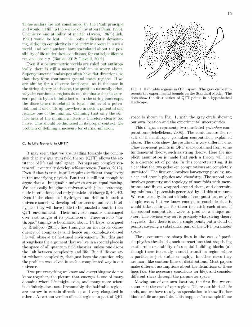
If we put everything we know and everything we do notknow together, the picture that emerges is one of manydomains where life might exist, and many more whereit definitely does not. Presumably the habitable regionsare narrow in certain directions, and very elongated inothers. A cartoon version of such regions in part of QFT

FIG. 1 Habitable regions in QFT space. The gray circle rep-resents the experimental bounds on the Standard Model. Thedots show the distribution of QFT points in a hypotheticallandscape.

space is shown in Fig. 1, with the gray circle showingour own location and the experimental uncertainties.

This diagram represents two unrelated gedanken com-putations (Schellekens, 2008). The contours are the re-sult of the anthropic gedanken computation explainedabove. The dots show the results of a very different one.They represent points in QFT space obtained from somefundamental theory, such as string theory. Here the im-plicit assumption is made that such a theory will leadto a discrete set of points. In this concrete setting, it isclear that the two gedanken computations are completelyunrelated. The first one involves low-energy physics: nu-clear and atomic physics and chemistry. The second oneinvolves geometry and topology of manifolds with mem-branes and fluxes wrapped around them, and determin-ing minima of potentials generated by all this structure.We can actually do both kinds of computations only insimple cases, but we know enough to conclude that itwould take a miracle for them to match each other, ifthe second computation were to produce a unique an-swer. The obvious way out is precisely what string theorysuggests: that there is not a single point, but a cloud ofpoints, covering a substantial part of the QFT parameterspace.

These contours are sharp lines in the case of parti-cle physics thresholds, such as reactions that stop beingexothermic or stability of essential building blocks (al-though there is usually a small transition region wherea particle is just stable enough). In other cases theyare more like contour lines of distributions. Most papersmake different assumptions about the definitions of theselines (i.e. the necessary conditions for life), and considerdifferent slices through the parameter space.

Moving out of our own location, the first line we en-counter is the end of our region. There our kind of lifeends, and we have to rely on speculation to know if otherkinds of life are possible. This happens for example if one

16

of the crucial processes in the functioning of stars is shutoff. Other processes may take over, but stellar lifetimesand/or heavy element abundances may differ by orders ofmagnitude, and we cannot rely on experimental data tobe certain that such a universe will “work”. Beyond thisterra incognita (perhaps more appropriately called “noman’s land”) there is usually another boundary where theconditions become so adverse that any kind of complex-ity can be ruled out. For a discussion along similar linessee Hall and Nomura (2008). In the rest of this reviewwe shall not make this distinction over and over again,and use the adjective “anthropic” rather loosely for anyparameter change that is likely to affect life, whether itis our life or life in general.

Real plots of this kind can be found in many papers,e.g. Agrawal et al. (1998b); Tegmark (1998); Hogan(2000); Tegmark et al. (2006); Hellerman and Walcher(2005); Graesser and Salem (2007); Hall and Nomura(2008); Barr and Khan (2007); Jaffe et al. (2009); Eloret al. (2010); and Barnes (2012).

Even without drawing further conclusions, it is simplyincredibly exciting to see where we are located on theparameter space map, and to see the lines of minor andmajor catastrophes surrounding us. It is a bit like seeingour fragile planet in the vastness of space, on the firstApollo 8 pictures. It is also a great way of appreciatinghow our universe really works. If we do indeed under-stand that, we should be able to change something andwork out the consequences.

Fig. 1 was deliberately drawn in this way to illustrate afew fallacies that are perhaps blatantly obvious, but thatare nevertheless repeated incessantly in the literature.

• Anthropic reasoning will never completely deter-mine the Standard Model. It is quite clear thateven in our own environment there are variationsthat have no conceivable impact on life, such as theτ mass. Furthermore, everything we know suggeststhat there might very well exist other, disconnectedhabitable regions, and even far in the foreseeablefuture our technical abilities will be insufficient torule them out.

• Anthropic reasoning combined with a fundamen-tal theory is not likely to determine the StandardModel either. This would require the density of thecloud to match the size of the anthropic region, insuch a way that precisely one point lands inside it.That would be another miracle.

• There is no reason to expect the maximum of thedensity distribution, even when folded with sam-pling probabilities, to select our vacuum. Comput-ing these maxima is another gedanken computationthat cannot be sensitive to the location of the do-mains, the other gedanken computation.

• The gray region decreases monotonically with time.Some people have tried to reduce arguments of thiskind to absurdity, by claiming that it leads to theconclusion that the density of points would haveto increase as well, in order to have a chance ofgetting one point inside the gray circle. But nocloud of points is needed to explain the presenceof one point in the experimental domain. There isno miracle here that requires such an explanation,because the experimental domain is not determinedby a calculation.

• Bounds on parameters may disappear as others areallowed to vary. Obviously the projection of the re-gions on the axes cover essentially everything, but ifwe intersect them with horizontal or vertical lines,we get narrow bounds. But that this was going tobe true was obvious from the start. In the (me,mτ )plane (keeping everything else fixed), the anthropicdomain is a extremely elongated along the mτ axis,and narrow along the me axis. If for some rea-son we decide that the fundamental parameters are(me −mτ ) and (me +mτ ) we would conclude thatif the latter linear combination is kept fixed, theformer is tightly constrained. Then someone mightpoint out that if (me+mτ ) was also allowed to vary,the bound goes away. People committing this obvi-ous fallacy are apparently either assuming that an-thropic arguments should constrain all parametersto a small circle, or do not understand the notionof small regions in more than one dimension.

If one can show that a parameter is anthropically con-strained, keeping all others fixed, that is a tremendoussuccess. If one can do it while allowing others to vary,that is an even bigger success. Only in cases where strongclaims are made about the actual value of a parameter(especially that it must be small), it becomes really im-portant to ask if the smallness is a consequence of fixingother parameters.

There is one interesting exception to the third point,namely if life in a universe somehow affects the samplingprobability of its offspring. This includes science fictionideas such as scientists making copies of their own uni-verse in experiments. Another variant was proposed by(Smolin, 1994), who argued that collapsing black holescreate new universes with slightly changed parameters,and that universes that are optimized for black hole pro-duction are also optimal for life. This would make themaximum of black hole production a point of attractionin a multiverse. But black holes are not a friendly en-vironment for life, nor a suitable device for transferringinformation. For further discussion see Rothman and El-lis (1993); Barrow (2001); Vilenkin (2006b); and Smolin(2006).

Note that any argument based on sampling probabili-ties, such as the one mentioned above, needs a landscape

17

of possibilities in the first place. Then the anthropic ge-nie is already out of the bottle. In any situation wherethe dots in Fig. 1 are sampled eternally, nothing elseis needed. Sampling probabilities, either determined byfundamental physics or by life itself, may help explain ourlocation within the anthropic domain, but cannot help inexplaining why we are inside a domain. The anthropicargument already explains that. Any second explanationjust creates a new mystery.

There exist numerous proposals for avoiding the an-thropic principle even given the existence of a huge land-scape, see for example (Bouhmadi-Lopez and Vargas Mo-niz, 2007; Brustein and de Alwis, 2006; Firouzjahi et al.,2004; Kawai and Okada, 2011; Kobakhidze and Mersini-Houghton, 2007; Linde and Vanchurin, 2010), but theytend to focus on one anthropic issue (in particular thecosmological constant), and ignore all others. For thecosmological constant, the value zero is a natural pointof attraction, and hence it is on quite general grounds nottoo surprising that it can be singled out by some mecha-nism. But this will not work for the more subtle, thoughfar less extreme tunings of the Standard Model, unless amiracle happens.

D. Levels of Anthropic Reasoning

Even in the interpretation used in this review, one maydistinguish several versions of the AP:

1. AP0: A mere tautology.

2. AP1: An explanation for certain fine tunings.

3. AP2: A predictive method.

AP0: If the fundamental theory allows many universesthat do not allow observers, we should not be puzzled tofind ourselves in one that does. This is true, but not veryuseful.AP1: Suppose we conclude that some variable x, a pri-ori defined on an interval [0, 1] has to lie in an extremelynarrow band of size ε for observers to exist. If the fun-damental theory contains N values of x evenly scatteredover the interval, the chance that none of them is in theobserver range is (1−ε)N . For N = M/ε and small ε thisgoes like e−M . For sufficiently large M , we would agreethat there is nothing surprising about the existence of apoint in the observer band. For concreteness, one maythink of numbers like 10−120 for ε and 10500 for N , sothat M = 10380. These are the kind of numbers thatappear in the discussion of one fine-tuned parameter, thecosmological constant. The chance that a flat distribu-tion contains no points in the observer range would thenbe the absurdly small number exp(−10380). Obviously,the fine-tuning is then explained. Note that we are talk-ing about landscape density distributions here, not about

sampling probabilities in eternal inflation (see section VIfor various approaches towards defining the latter).

AP2: It may be possible to go one step further, anddetermine the most probable point where we should ex-pect to find ourselves within the anthropic window. Thisrequires additional information compared to AP1. Weshould be able to assign a probability to each point, workout the probability distribution, and determine its max-imum. We need to know how often a certain solutionis sampled with respect to others, and we will have tocompare the “fertility” of distinct universes that allowobservers. Universes with more observers are more oftenobserved.This brings some very serious measure prob-lems into the discussion. What counts as an observer,and what counts as an observation? Should we sum overthe entire history of the universe, and how do we includeparts of the universe that are currently behind the hori-zon? How do we even define probabilities in the contextof eternal inflation, where anything that can happen hap-pens an infinite number of times? Furthermore there isthe issue of “typicality” (Vilenkin, 1995a). If we can de-fine and compute a probability distribution, should weexpect to find ourselves at its maximum? Are we “typi-cal”? Does statistics even make sense if we can observejust a single event?

Many criticisms of anthropic reasoning are aimed atthe measure and typicality problems in AP2, and espe-cially its use for predicting the cosmological constant. Seefor example Armstrong (2011); Bostrom (2007); Maoret al. (2008); Muller (2001); Neal (2006); Smolin (2004);and Starkman and Trotta (2006) for a variety of thoughtson this issue. We will return to the measure problem insection VI.

Sampling probabilities are not relevant for AP1. Sup-pose xa is a value of x for which observers can exists,whereas for xb they cannot exist. If N is much smallerthan 1/ε the existence of a habitable value xa in thefundamental theory is mysterious. This becomes no lessmysterious if xa has a vastly larger sampling probability.Would we conclude that we find ourselves in xa becausethat is far more probable, or because nothing can live inxb? Similarly, if xb had a much larger sampling proba-bility, would that affect the conclusion in any way?

Perhaps AP1 is as far as we can ever get. We maydetermine the boundaries of our domain, and find outhow a fundamental theory spreads its “vacua” over thatdomain. There is a lot of interesting physics and math-ematics associated with all of these questions. In theend we may just be satisfied that we roughly understandwhere we are, just as we are not especially obsessed withderiving the orbit and size of our planet in the landscapeof astrophysical objects. Establishing the fundamentaltheory will have to be done by other means, perhapspurely theoretically, and by ruling out alternatives.

18

Sharp predictions, rare even in the golden age of par-ticle physics, are not likely to come from this. An AP1-based prediction would say nothing more than that welive within an anthropic domain, and almost by definitionthat can never be more than a post-diction. AP2-basedpredictions may be possible in cases where some con-tribution to the probabilities is strongly skewed in onedirection. In that case we may predict that we shouldlive close to the edge of an anthropic domain, or the in-tersection point of several edges.

In the context of a multiverse sampling the string land-scape the “anthropic principle” is nothing more than abias we have because we exist as observers. Therefore itmakes no sense to ask if the anthropic principle is falsi-fiable or require that it makes any predictions. It is theunderlying theory that has to be falsifiable.

e. Measures of fine-tuning It is impossible to make amathematically precise statement about the amount of(fine)-tuning. To compute the surface areas we need ameasure on the space of quantum field theories, but thisspace does not come with a measure. By “measure” wemean here a prescription to compute a surface area inFig. 1 in order to decide that an anthropic region is largeor small. This should not be confused with the measureproblem of eternal inflation (see section (VI.B), whichhas to do with the relative sampling rates of vacua.

The most common situation is that of a dimension-ful parameter that is small in Planck units, such as thestrong scale (or the proton mass), the weak scale or thecosmological constant. If one assumes a flat distributionone may say that the parameter is fine-tuned. But ifinstead we use a logarithmic distribution the conclusionwould be different. If the proton mass must be as smallas it is for anthropic reasons, we need to tune it with 19digit precision if the distribution is flat, but with onlytwo digit precision if we only need to tune the exponent.

Therefore it is rather pointless to ask if our universeis “fine-tuned” as long as we only know one vacuum. Ina sufficiently dense discrete landscape this question be-comes well-defined: the discrete points provide a mea-sure. But if the existence of a discrete landscape hasalready been established, the question looses much of itsrelevance.

E. First Signs of a Landscape?

Historically, we are in a remarkable situation. TheStandard Model is consistent, and can be extrapolatedall the way to the Planck scale. Our vacuum may bemetastable, but this is not an inconsistency nor a dis-agreement with any experimental result. We have a com-plete theory of the strong electromagnetic and weak in-teraction that seems to be perfectly adequate. All re-

maining problems of the Standard Model are matters oftaste. There are many unmotivated choices, and manydimensionless parameters are very small. It is worth em-phasizing this point because this is a rare moment in thehistory of physics that may already have passed whenthis review appears in print.

The current situation in particle physics invites an ap-peal to Occam’s razor. Although there are shelves full ofscientific work proposing new physics beyond the Stan-dard Model, it is strange that all of that new physics hasmanaged to hide itself so well. Perhaps nature is playinga really evil trick with us, presenting us with a completeStandard Model just to deceive us. But we cannot avoidasking the obvious question: Could it be that the Stan-dard Model, including a minor extension to accommodateneutrino oscillations, is really all there is? Indeed, sug-gestions in that direction have already been made sometime ago by Shaposhnikov and Tkachev (2006), albeitnot in the context of a landscape.

It is undeniable that this state of affairs has con-tributed to the interest in “anthropic” and “landscape”thinking in particle physics. Could it be true that theStandard Model is like a dart that was thrown repeat-edly at the space of all quantum field theories, until oneof them landed in one of the anthropic domains of Fig.1? This is the central question of this review.

It is clear that the discovery of major new structures,especially new strong interactions, would indicate thatthis sort of thinking is, at best, premature. But thiswould also raise the alarming possibility of an indefiniteseries of matryoska’s of substructure, which we mightnever be able to disentangle completely. Would that be amore attractive option than a landscape? The absence ofmajor new physics in any accelerator experiment in thelast decade may be an indication that we are living ata special time in the history of particle physics, that wemight have our first view of the foothills of a landscape.Perhaps we have reached the interface of bottom-up andtop-down thinking, and our next task is to locate theStandard Model of particle physics within the landscapeof some fundamental theory, perhaps string theory.

Low energy supersymmetry, by far the most discussedoption for new physics, is an attractive compromise.It might be the final step towards a theory of all in-teractions, allowing a smooth interpolation towards thePlanck scale, and could give us important clues aboutthat theory. Nothing we know about low energy super-symmetry gives evidence against the idea of a landscape.It does not reduce the number of parameters, quite thecontrary, and supersymmetry itself plays a crucial rolein understanding the only (part of) a landscape we caneven begin to discuss. But if nature wanted to provide uswith a soft, supersymmetric, landing on the landscape,it could have given some clues a little earlier.

But even in the most extreme landscape scenario, thereare plenty of problems left that require a solution. It is

19

just that the nature of the remaining problems has shiftedin a remarkable way in a certain direction: most prob-lems are now “environmental”, and many have anthropicimplications.

One can roughly order the open problems according totheir urgency, in the following way.

• No consistent theory.

• Disagreement between theory and experiment.

• Environmental, but not anthropic problems.

• Potentially anthropic problems.

We will make an – admittedly rather artificial – sepa-ration between particle physics and cosmology.

1. Particle Physics

The main item in the first category is quantum grav-ity. The Standard Model does not contain gravity, andadding it using standard QFT methods leads to incon-sistencies. Some people would argue that a violation ofthe stability bound on the Higgs self-coupling belongs inthis category as well.

In the second category there is a long list of deviationsof low statistical significance that may one day developinto real problems, astrophysical phenomena for whichthere is no good theoretical model, but which may pointto new particle physics, a hint of a gamma-ray line incosmic rays at 130 GeV (Weniger, 2012) and a 4σ indi-cation for spatial variations of the fine structure constant(Webb et al., 2011).

The last two categories refer to the so-called “why”problems: why are certain parameters or discrete choicesthe way they are. This kind of problem may never besolved. Nothing goes wrong if we cannot find a solution,and there is no experiment we can do to force nature togive us a clue. If in addition different values of a parame-ter have a negative impact on the prospects for life, thenthis fact already provides a clue. Then it becomes evenless obvious that a “solution”, in the traditional sense, isrequired. But we should not jump to conclusions. Sim-ply saying “parameter X has value y, because otherwisewe would not exist” is too simplistic.

In the third category are all Standard Model param-eters that have peculiar values, without any reason tohope that anthropic arguments are going to be of anyhelp. The most important one is the CP-violating angleθ of the strong interactions, arguably the most impor-tant Standard Model problem in the context of a land-scape (Banks et al., 2004; Donoghue, 2004). Anotherexample of non-anthropic parameters with small valuesare the CKM angles, and some of the quark mass ra-tios. The famous questions “why are there three familiesof quarks and leptons” is probably in this category as

well, although the number “3” is not very peculiar froma landscape perspective, so this does not even belong ona list of problems.

The last category consists of all problems related toparameters whose values do potentially have an impacton the existence of life. This includes the group structureand representations of the Standard Model, the scales ofthe strong and the weak interactions (the “gauge hier-archy problem”, see subsection V.C.2), the light quarkmasses and the electron mass (assuming the heavierfermions stay heavy), neutrino masses and perhaps eventhe mass of the top quark. The environmental impact ofthe fermion masses will be discussed in section V.B.

2. Cosmology

For the sake of the argument we will treat cosmologyas a theory with input parameters, although its theoreti-cal underpinnings are far less robust. There are certainlyplenty of “category 1” problems here, especially in infla-tion and pre-big bang cosmology. For Standard Modelparameters it is easier to accept the extreme form of thelandscape paradigm, namely that the Standard Modelmight be merely a point in a huge landscape about whichonly few details can be derived from fundamental physics,just as only a few general features of Mount Everest canbe derived from geology. In cosmology we are simply notin such a situation, or at least not yet.

The main cosmological parameters are the cosmologi-cal constant Λ, the density parameter Ω, the matter den-sity fluctuations Q = δρ/ρ, the dark/baryonic matterratio ζ, the baryon-to-photon ratio η and the parame-ters of inflation (see Tegmark et al. (2006) for a system-atic survey of all parameters). There is no effectivetheory of cosmology where all of these parameters canmanifestly be varied independently and without worry-ing about the impact of changes in our understanding ofgravity. For example, the cosmological constant only hasan observable meaning in a theory of gravity. The notionof decoupling it from gravity, as one can do for StandardModel parameters, does not even make sense. Cosmo-logical variations are highlighted in the book “Just SixNumbers” (Rees, 1999); just one of his six numbers, thefraction of energy released in nuclear reactions, is directlyrelated to Standard Model physics.

Anthropic issues in cosmology will not be discussedin detail in this review, except for the cosmological con-stant, the focal point of a lot of attention. Here we willjust briefly mention some interesting observations.

The main item in the second category is “dark mat-ter”, or more precisely the complete set of problems thatis elegantly solved if we postulate the existence of darkmatter: galaxy rotation curves, the bullet cluster, struc-ture formation, the features of the Cosmic MicrowaveBackground (CMB), the amount of deuterium produced

20

in Big Bang Nucleosynthesis and the matter density ofthe Universe. There is a minority point of view that holdsthat these problems belong in the first category, and re-quire a modification of gravity. But should we really beso surprised if dark matter exists? Is it not a typicalexample of anthropocentric hubris to assume that any-thing that exists in the universe must be observable byus, or made out of the same stuff that we are made of?Postulating dark matter moves this problem largely tocategory four, although there are still serious problemsin computer simulations of galaxy formation which maypoint to a more fundamental problem (see Famaey andMcGaugh (2013) for a list of open problems).

The dark-to-baryonic matter ratio ζ, which is ≈ 5 inour universe, may have anthropic implications, since darkmatter plays an important role in structure formation.This was first discussed for axion dark matter (Linde,1988), because the most popular solution to the strongCP problem, the Peccei-Quinn mechanism, predicts anadditional particle, the axion, that contributes to darkmatter. In contrast to the more popular WIMP darkmatter2, whose abundance is predicted by its interac-tions, axionic dark matter must satisfy constraints whichare in part anthropic in nature (for more on axions seesection V.D). The constraints were made more precise byHellerman and Walcher (2005), who found ζ < 105 andTegmark et al. (2006) who concluded that 2.5 < ζ < 102,using some additional anthropic requirements. These pa-pers also discuss the effect of other parameter variations(in particular Q and Λ) on these bounds. Using assump-tions about a multiverse measure and the number of ob-servers per baryon, Freivogel (2010) gave an anthropicstatistical prediction for ζ roughly in agreement with theobserved value. Although the emphasis on all these pa-pers is on axionic dark matter, some of the conclusionson ζ do not really depend on that.

Most other cosmological parameters are also in thefourth category. Changing any of these substantially hasan impact on some feature in the history and/or currentstatus of the universe that would appear to be catas-trophic at least for our kind of life, and hence it is atleast possible that this is part of the reason we observethe values we do.

But once again, we should not jump to conclusions.An extreme example is the smoothness and isotropy ofthe cosmic microwave background. This fact may be re-garded as environmental, and if it were a wildly fluctu-ating distribution this could have a very negative impacton the prospects for life (Tegmark and Rees, 1998). Butsurely one cannot assume that the entire density pertur-bation function is tuned this way just for life to exist

2 WIMPs are “weakly interacting massive particles”, which arepresent, for example, in certain supersymmetric extensions ofthe Standard Model.

in one galaxy. The most popular solution to this “hori-zon problem” is inflation, which solves another problemwith anthropic relevance, the flatness problem, but alsointroduces some new fine-tunings.

Inflation is an especially rich area for anthropic andlandscape ideas. An early example is Vilenkin (1995a),giving arguments that typical civilizations will see an ex-tremely flat inflaton potential. In Freivogel et al. (2006)anthropic landscape arguments are given suggesting thatthe number of e-folds of inflation will not be much largerthan the observed lower bound of about 60. Accordingto these authors, 59.5 e-folds are required for structureformation, and we should not expect to see much morethan that.

Many features of string theory have the potential to berelevant here such as moduli, axions (Dimopoulos et al.,2008) and D-branes (Kachru et al., 2003a). In Liddle andUrena-Lopez (2006) the possibility of a common originof inflation, dark matter and dark energy in the stringlandscape is discussed. See Burgess (2007); Cicoli andQuevedo (2011); Kallosh (2008); and Quevedo (2002) forreviews of inflation in string theory. But inflation in thestring landscape also introduces new problems, see e.g.Allahverdi et al. (2007); Hall et al. (2006); and Huangand Tye (2009).

Inflationary cosmology also offers interesting opportu-nities for predictions of features of the CMB, see e.g.Ashoorioon (2010); Frazer and Liddle (2011); Holmanet al. (2008); Tegmark (2005); and Yamauchi et al.(2011). Furthermore, the CMB may even give directhints at the existence of a multiverse. There is a chance ofobserving collisions with other bubbles in the multiverse,see for example Aguirre et al. (2007) and WMAP resultspresented by Feeney et al. (2011). Gonzalez-Dıaz andAlonso-Serrano (2011) consider an even more exotic pos-sibility involving non-orientable tunneling. In principlethere might be information about other universes in thedetailed structure of the cosmic microwave background,but at best only in the extreme future (Ellis, 2006b).

Anthropic predictions for the density parameter Ω werealready made a long time ago by Garriga et al. (1999).This work, as well as Freivogel et al. (2006), points outthe plausibility of observing negative spatial curvature,(i.e. Ωk > 0, where Ωk ≡ 1 − Ω) in a multiverse pic-ture. They argue that sixty e-folds of inflation are an-thropically needed, and having a larger number of e-folds is statistically challenged. The current observa-tional constraint is |Ωk| < 10−2. Furthermore, Guthand Nomura (2012) and Kleban and Schillo (2012) pointout that observation of even a small positive curvature(Ωk < −10−4) would falsify most ideas of eternal infla-tion, because tunneling in a landscape gives rise to openFriedmann-Robertson-Walker (FRW) universes.

That the baryon to photon ratio η ≈ 6 × 10−10 mayhave anthropic implications was already observed a longtime ago (see Carr and Rees (1979); Nanopoulos (1980);

21

Linde (1985) but also Aguirre (2001) for critical com-ments), but it is not simply a tunable free parameter.Inflation would dilute any such initial condition, as wouldany baryon number violating process that gets into equi-librium in the early stages of the universe. See Shaposh-nikov (2009) for a list of 44 proposed solutions to thebaryogenesis problem. Most of these solutions generatenew anthropic issues themselves.

This brief summary does not do justice to the vastbody of work on string and landscape cosmology. Furtherreferences can be found in reviews of string cosmology,e.g. Burgess and McAllister (2011).

3. The Cosmological Constant

The cosmological constant Λ is a parameter of classicalgeneral relativity that is allowed by general coordinate in-variance. It has dimension [length]−2 and appears in theEinstein equations as (the metric signs are (−,+,+,+))

Rµν −1

2gµνR+ Λgµν = 8πGNTµν . (3.1)

Without a good argument for its absence one shouldtherefore consider it as a free parameter that must be fit-ted to the data. It contributes to the equations of motionwith an equation of state P = wρ, where P is pressureand ρ is density, with w = −1 (matter has w = 0 andradiation w = 1

3 ). As the universe expands, densities arediluted as (the initial values are hatted)

ρw = ρw

(aa

)−3(1+w)

. (3.2)

As a result, if Λ 6= 0 it will eventually dominate if theuniverse lasts long enough (and if there is no “phantommatter” with w < −1).

However, Λ itself affects the expansion. For Λ < 0the universe collapses in a time ct = π

√3/Λ whereas

for Λ > 0 the universe goes into exponential expansionas exp(

√Λ/3ct). These two cases correspond to exact

maximally symmetric solutions to the Einstein with Λ 6=0 and without matter, and are called Anti-de Sitter (AdS)and de Sitter (dS) spaces respectively. The latter has ahorizon at a distance (

√Λ/3 from the observer. Light

emitted by matter beyond that horizon can never reachthe observer because of the expansion. The fact thatour universe has existed billions of years and that weobserve galaxies at distances of billions of light years givesimmediately an upper limit on |Λ| (see Eq. (3.4) below)which is already known for decades (Barrow and Tipler,1986)).

The fact that the length associated with Λ is of cos-mological size is not surprising in itself, but there issecond interpretation of Λ that puts this in an entirelydifferent perspective. The parameter Λ contributes to

the equations of motion in the same way as vacuum en-ergy density ρvac, which has an energy momentum ten-sor Tµν = −ρvacgµν . Vacuum energy is a constant con-tribution to any (quantum) field theory Lagrangian. Itreceives contributions from classical effects, for exampledifferent minima of a scalar potential and quantum cor-rections (e.g. zero-point energies of oscillators). How-ever, it plays no role in field theory as long as gravityis ignored. It can simply be set to zero. Since vacuumenergy and the parameter Λ are indistinguishable it iscustomary to identify ρvac and Λ. The precise relation is

Λ

8π=GNρvac

c2:= ρΛ . (3.3)

This immediately relates the value of Λ with all otherlength scales of physics, entering in ρΛ, which of courseare very much smaller than the size of the universe. Theextreme version of this comparison is to express ρΛ inPlanck mass per (Planck length)3, which gives a valuesmaller than 10−120. This was clear long before ρΛ wasactually measured.

This huge difference in length scales implies a hugefine-tuning problem. It was noted a long time ago by(Linde, 1974; Veltman, 1975) that the Standard ModelHiggs mechanism induces a huge change in vacuum en-ergy. Other contributions are expected to come from dy-namical symmetry breaking in QCD and inflation. Thelatter is especially hard to avoid, because in most mod-els the exponential is driven by vacuum energy, whichmust therefore have been vastly larger in the inflationaryperiod than it is now. Quantum corrections to vacuumenergy are due to vacuum bubble diagrams (coupling togravitons to generate the

√−g factor). There are contri-

butions from all particles, with opposite sign for bosonsand fermions. These diagrams are quartically ultra-violetdivergent: they are infinite if we naively integrate overarbitrarily large momenta, and they are proportional toM4

cutoff if we assume that nature cuts off the divergenceat some scale M4

cutoff (note that that quantum correc-tions contribute to the density ρvac, and hence Λ getsquartic corrections, not quadratic ones as its dimensionmight suggest). It is likely that the divergent integral arecut off by a consistent theory of quantum gravity (andindeed, string theory does that), and in that case thecut off scale would be the Planck scale. In that case, thenaive order of magnitude for ρΛ is the Planck density, onePlanck mass per Planck volume (5.15× 1096 kg/m3). Inthese units the aforementioned old observational limits,using y × 109 (light)years for the assumed cosmic time(length) scale, are3

|ρΛ| < 3.4y−2 × 10−121 (3.4)

3 In the rest of this section we use ~ = c = GN = 1.

22

The fact that this number is so absurdly small is called“the cosmological constant problem”. The problem canbe mitigated by assuming a smaller cutoff scale for thequantum corrections, but even if we choose the TeV scalethere are still sixty orders of magnitude to be explained.It seems unlikely that the cut-off can be less than that,because then we are in known quantum field theory ter-ritory, and furthermore we then have the classical con-tributions to worry about as well. One may considerradical changes to the theory, so that gravity somehowdoes not couple to vacuum energy at all, but so far noworking proposals exist. See for example (Bousso, 2008;Polchinski, 2006; Weinberg, 1989) for a summary of someof these ideas and why they do not work.

A recent very detailed review is (Martin, 2012). Thispaper, just as (Koksma and Prokopec, 2011) makes theremarkable claim that vacuum energy diagrams are notdivergent in quantum field theory, but finite and pro-portional to m4ln m, with opposite signs for bosons andfermions, and vanishing contributions for photons andgravitons. This would still get us only halfway (there arestill vacuum contributions, a bare contribution, and theloop contributions do not magically cancel). The trou-ble with this claim is that, even if correct, it requiresknowing the full particle spectrum at all mass scales.If QED is embedded in a GUT, there would be extraGUT particles contributing, and the claim that photonsdo not contribute to vacuum energy looses its meaning.The whole point of renormalization is that everythingunknown beyond a certain mass scale is combined intoa few constants, such as Λ. This proposal violates thatprinciple. It can only be useful if we know the completetheory, but in that case we would also know Λ. This justillustrates how hard it is to get rid of contributions fromvacuum diagrams.

The small observational limit led most people to be-lieve that Λ had to be identically zero, for reasons thatwere still to be discovered. But then from observationsof redshifts of distant type-Ia supernovae gave evidencefor accelerated expansion (Perlmutter et al., 1999; Riesset al., 1998). This expansion can be fitted with the Λ-parameter. Combined with more recent data on the cos-mic microwave background this indicates that the contri-bution of Λ to the density of the universe is about 70%of the critical density ρc ≈ 9.9 × 10−27kg/m3, assumingthe standard ΛCDM model of cosmology. Then

ρΛ ≈ +1.3× 10−123 (3.5)

a. Anthropic arguments. The foregoing discussion al-ready implies that there will be an anthropic range forΛ, assuming everything else is kept fixed. Although thismay have been clear to some much earlier, it appears thatthe first paper stating this is Davies and Unwin (1981).

They did not make it quantitative, though. In subse-quent years Banks (1985); Linde (1984); and Sakharov(1984) also discussed anthropic implications of Λ 6= 0.Sakharov’s paper contains the remarkable statement: “Ifthe small value of the cosmological constant is determinedby “anthropic selection”, then it is due to the discreteparameters. This obviously requires a large value of thenumber of dimensions of the compactified space or (and)the presence in some topological factors of a complicatedtopological structure.”

Since Λ must be small to get a large cosmologicallength or time scale, it is obvious that Λ is anthropicallybounded in any universe that has life based on some kindof nuclear or chemical complexity, for any underlying fieldtheory. If one requires that a compact object consistingof N constituents of mass µ (in Planck units) fits insidea dS horizon, one gets Λ . µ2N−2/3 . N−4/3, wherethe second inequality holds for pressure-balanced objects(stars, planets or humans, but not galaxies). In AdSspace the minimal time for biological evolution, somelarge number M times the constituent time scale µ−1,must be smaller than the collapse time, ≈

√3/Λ. This

gives a limit −Λ .M−2µ2. Clearly, both N and M mustbe large but are not computable from first principles; inour universe N ≈ 1027 for a human brain and M 1031

(assuming full biological evolution in a single year). IndS space a better limit can be obtained by weakening theassumptions underlying Weinberg’s argument or by de-termining the maximal size of an object that can breakaway from the exponential expansion. Using results fromHellerman and Walcher (2005), Harnik et al. (2006) de-rived a limit

ρΛ . min[µ4, µ−2N−2

](3.6)

No matter which limit one uses, the conclusion is in anycase that in universes with a value for Λ that is not ex-tremely small life is impossible. Obviously these are verycrude limits, and there is no guarantee that other uni-verses exist where |ρΛ| is as large as one of the bounds.But, crude as it may be, this arguments implies that ifΛ can be treated as a free parameter on a Planckian in-terval, it is clearly true that the reason for its smallnessis anthropic.

If all other parameters are kept fixed at their observedvalues, much tighter bounds can be obtained. Barrowand Tipler (1986) pointed out that if Λ is too largeand negative, the universe would collapse before life hasevolved. The precise limit depends on the time neededfor stars to produce heavy elements, and the time neededfor biological evolution, for which we have no theoreticalestimate, and just one data point. The authors used theaverage life-time of a main-sequence star to get a limit.This quantity can be entirely expressed in terms of Stan-dard Model parameters and the Planck mass, and leads

23

to a limit

|ρΛ| / α−4

(me

mp

)4(mp

MPlanck

)6

= 6.4× 10−120. (3.7)

For negative Λ the collapse of the entire universe is un-questionably a limit, but there are still some importantuncertainties in this bound. Because we have observa-tional evidence for a positive Λ, the bound for negativeΛ may seem irrelevant, but it is interesting for severalreasons, so it is worthwhile to see if it can be made moreprecise. The formula on which it is based is actually theEddington limit, a lower limit on the lifetime for objectsradiating at maximum luminosity. This limit is

Tmin =2

3ε

[(MPlanck

mp

)3]α2m2

p

m2e

tPlanck ≈ 3 million years

where ε is the energy efficiency, the fraction of mass thatcan be converted to energy, ε ≈ .007. The actual limit isequal to ttot = t∗ + tev, where t∗ is the time of the firstsupernova explosion after the big bang (which producedthe required heavy elements) and tev the shortest timeneeded for geological and biological evolution. The lattercannot be determined from first principles. It dependson biological time scales, the evolution of the sun, platetectonics, volcanism, the movement of the solar systemthrough the spiral arms of the galaxy, subtle variationsin the earth’s axis, the moon, Jupiter, meteor impactsand other catastrophic events, effect we do not even knowabout, and most importantly, chance. From the one datapoint we have we know that 13.8 billion years is sufficient.If we assume that we are typical, faster evolution mustbe far less probable, but as long as it is possible it affectsthe limit. The most conservative assumption is that tev

under ideal circumstances could be less than a millionyears, so that the limit is determined by the minimalstellar lifetime. So ttot, the minimal time between the bigbang and evolution until intelligent life, must lie between3 million years and 13.8 billion years. Requiring thatthis is less than the time of collapse, π

√3/Λ, gives ρΛ >

−ρmin, with

1.8× 10−122 < ρmin < 3.8× 10−115 . (3.8)

The limit (3.7) was argued to be valid for positive Λ aswell. However, Weinberg (1987) pointed out that struc-ture that has already formed will not be ripped apartby an expanding universe. Once galaxies have formed,it makes no difference how much time is needed to makestars or evolve life, because the expansion will not inhibitthat from happening. He then derived a limit based onthe assumption that life would not form if the universeexpands too fast to inhibit galaxy formation. The exactform of Weinberg’s bound is

ρΛ <500

729∆3ρ0 , (3.9)

and was derived by studying the collapse of a sphericaloverdensity ∆ using a Robertson-Walker metric. Theoverdensity starts expanding at t = 0 when the universehas a matter density ρ0. For ρΛ = 0 it recollapses andforms structure, but as ρΛ is increased a point is reachedbeyond which the recollapse does not occur anymore.This gives the maximum value of ρΛ for the overdensity∆. The absolute upper limit in a given universe is givenby determining the maximal overdensity that can occur.Since density fluctuations are distributions, there will notbe a strict upper limit, but the number of galaxies thatcan be formed will drop off rapidly beyond a certain ρΛ.

A “lower bound on the anthropic upper bound” can beobtained by observing quasars (centers of young galaxies)at high redshift z, and then extrapolating the observedmatter density back to the corresponding age by multi-plying the present ρmatter by a factor (1+z)3. If we know,empirically, that galaxies can form at such densities, thenvacuum density can not play a role if is smaller than thedensity of matter. With the information available in 1987this argument gave an upper limit of at least 550ρmatter

based on quasars observed at z = 4.4 (the exact pre-factor is 1

3π2(1 + z)3). However, meanwhile dwarf galax-

ies have been observed at z = 10, increasing the boundby almost an order of magnitude (Loeb, 2006). The ob-served value of ρΛ/ρmatteris about 2.5, more than threeorders of magnitude below this upper bound. There isalso an upper bound to this upper bound: at a redshiftof z ≈ 1000 we reach the time of decoupling, and we arecertainly not going to observe galaxies that formed thatearly. This implies an absolute upper limit on ρΛ of order10−113.

b. Estimates of the Value of Λ. Nowadays we can deter-mine the density fluctuations using COBE and WMAP(and recently PLANCK) results. It is instructive tomake a rough estimate using the time of matter-radiationequality as the starting point of structure formation. Anorder of magnitude estimate for the matter density atequality is (Hellerman and Walcher, 2005): ρeq ≈ T 4

eq,Teq ≈ mpη(ζ + 1), where η = 6.3× 10−10 is the baryon-to-photon ratio and ζ the cold dark matter to baryonratio. Using for ∆ the average for the fluctuations,Q ≈ 2 × 10−5 yields ρΛ < 7.3 × 10−125 (with parame-ter values from Tegmark et al. (2006)). Putting in thecorrect factors of order 1, and taking into account thecontribution of neutrinos to matter-radiation equality,lowers this number substantially. Clearly a more carefultreatment of galactic-size density perturbations (whichcontribute with a third power) is needed.

Furthermore the “bound” is not a step function. Oneexpects a mean density of galaxies that falls of with in-creasing ρΛ. Such a function was computed by Efstathiou(1995) based on the results of COBE (but prior to theobservation of accelerated expansion). Although the ob-

24

servation of a positive Λ in 1998 came as a shock tomany, there were already several indications in that di-rection because of the density contribution needed forspatial flatness (as predicted by inflation) and the ageof the universe. This had already been pointed out byWeinberg (1987). The results of Efstathiou (1995) pre-dicted a value for ρΛ in agreement with that expectation,although with large uncertainties, and subject to somecriticisms (Vilenkin, 1995b; Weinberg, 1996). This com-putation was improved and done analytically rather thannumerically by Martel et al. (1998), with similar results.Distributions for ρΛ based on more recent cosmologicaldata can be found in Pogosian and Vilenkin (2007) andTegmark et al. (2006).

Computations of this kind rely on several assump-tions. The distribution of theoretically allowed valuesof ρΛ must be essentially flat near Λ = 0. Since Λ = 0is not a special point from the perspective of quantumgravity, and since the relevant range is extremely smallin Planck units, this seems plausible. Furthermore, thevacuum selection mechanism – for example eternal infla-tion – must not prefer special values either. This is lessobvious, see section VII. It is assumed that observersare correlated with galaxies, and sometimes with stars,planets and baryons, and that we are typical observers(the “principle of mediocrity” of Vilenkin (1995a)).

The computations mentioned above assumed that onlyρΛ varies. The possibility that Q also varies was consid-ered by Tegmark and Rees (1998), who computed the an-thropic bounds 10−6 < Q < 10−4 assuming Λ = 0. Theyalso pointed out that without anthropic bounds on Q,the bound on Λ is invalid. A potentially serious problemwas raised in Banks et al. (2004); Graesser et al. (2004);Garriga and Vilenkin (2006); and Feldstein et al. (2005).Depending on models of inflation, the probability distri-bution may vary so steeply as a function of Q that ex-treme values are strongly preferred, so that the observedvalue Q ≈ 10−5, roughly in the middle of the anthropicrange, has a very low probability of being observed (the“Q-catastrophe”). But even when both ρΛ and Q vary,there is a robust bound on ρΛ/Q

3 (Garriga and Vilenkin,2006). See Vilenkin (2004) for a brief review of anthropicpredictions for the cosmological constant.

We return briefly to the cosmological constant problemin section VII, after the string theory landscape and themeasure problem have been explained.

F. Possible Landscapes

1. Fundamental Theories

The “Anthropic Principle” discussed here is not a prin-ciple of nature, and not our ultimate goal. That goal isa fundamental theory in which different quantum fieldtheories are realized, and can be sampled.

We are not interested in an anthropic principle addedto the Standard Model and General Relativity as an ad-ditional principle of physics. The ultimate goal remainsfinding a “theory of everything”, a theory that agreeswith all current experiments and can be extrapolatedto extreme limits without encountering inconsistencies.

This fundamental theory provides the input distribu-tions for anthropic arguments, and may in principle befalsified with the help of such arguments. But it is thefundamental theory we should try to falsify, and not theanthropic principle, which is only a tool that may helpus finding the theory. Once that has been achieved, theanthropic principle will only be a footnote.

In the rest of this review we will avoid the term “the-ory of everything”, since it sounds a bit too pretentious,and just call it a “fundamental theory”. But whateverit is called, one can raise a number of objections. Per-haps such a theory does not even exist, or perhaps ourmental abilities are too limited to find it, or perhaps wesimply do not have enough information to figure out theanswer. Since, by assumption, we can only extract all ourinformation from an infinitesimal bubble in a multiverse,the latter possibility is a very serious one. One can alsospeculate about fundamental obstacles, along the linesof Goedel’s theorem or Heisenberg’s uncertainty princi-ple that would make it impossible, in principle to everachieve such a goal. Or one may believe in the onionshell paradigm, which states that as we explore nature atever shorted distances, we will continue to discover newphysics forever, like peeling layers from an onion with aninfinity of shells. But most physicists believe that therewould be a last shell at the Planck length, so that thenumber of unknown shells is presumably finite.

The marvelous success of the Standard Model givessome reason for optimism. It might even turn out to bethe last shell. It brings three of the four known interac-tions under control, and hence it seems not too unreason-able to hope that the fourth one can also be mastered.The first attempts to apply the traditional methods ofperturbative quantum field theory to quantum gravitywere made decades ago (’t Hooft and Veltman, 1974) butran into problems. String theory can be considered themost conservative attempt to overcome these problems.It does indeed overcome them in special cases (ten space-time dimensions with supersymmetry). There are goodreasons to believe that in that case it does indeed leadto the desired finite perturbative expansion. But that isnot all we expect from a fundamental theory.

If one accepts the foregoing anthropic arguments, it isnot plausible that the Standard Model is mathematicallyunique. Nothing said so far about a possible fundamen-tal theory requires that. Non-uniqueness of the StandardModel may look like the end of last century’s dreams, butit is only saying that those dreams were to naive. Thenwe need a fundamental theory which allows several, pre-sumably a large number, of alternatives. In general, we

25

will refer to the list of options as the “landscape” of thattheory. This list consists of all universes like our own(which of course must be on the list itself), but with adifferent point in the space of all quantum field theoriesgoverning matter and the non-gravitational interactions.In string theory we can – in some cases – give this no-tion a more precise meaning, where the different pointscorrespond to minima of a potential. The name “land-scape” was, presumably, partly inspired by the hills andvalleys of that potential, as well as by the common usagein other fields, such as the “publishing landscape”.

But we will need more than just a list of options. Therehas to be a way to reach different points in that landscapethrough some kind of physical process, such that they canall be sampled in a process like eternal inflation. Thisdisqualifies the quantum field theory landscape, whereany QFT is allowed, but there is no mechanism to gofrom one to another.

2. The role of gravity

During three-quarters of last century, particle physicsand gravity where mostly treated as separate subjects.All Lorentz covariant theories of particle physics can becoupled straightforwardly to classical general relativity.Furthermore, gravity can be consistently decoupled fromparticle physics by sending Newton’s constant to zero.The fact that quantum gravity did not enjoy the sameconsistency as quantum field theory (in particular the ex-istence of perturbative infinities that cannot be removedby renormalization) was often stated, but seen mostly asa problem of gravity. On the other hand, the remain-ing problems of particle physics – understanding the dis-crete and continuous choices of groups, representationsand parameters – have often been thought to be com-pletely solvable without coupling to gravity. This mightindeed be true. However, there are good grounds to be-lieve that these two theoretical areas must meet.

Indeed, there are a few concrete reasons why one mightexpect (quantum) gravity to play a role in limiting thenumber of options of quantum field theory.

UV completion. The renormalization procedure thatworks so well in quantum field theory requires an in-finite number of fundamentally undetermined parame-ters in quantum gravity. Although in all low-energy ob-servables their contribution is suppressed by powers ofthe Planck mass, this situation is untenable in a theorythat aims at determining the Standard Model parame-ters. Furthermore one cannot solve this problem in grav-ity alone. Gravity can be decoupled from the StandardModel, but not the other way around. Loop correctionsdue to matter are equally important as loop correctionsdue to gravity itself. One has to find a theory of matterand gravity that does not have these problems. This is

the requirement of “UV completeness”. One may expectthis to restrict the possibilities for matter.

Vacuum energy. The energy of the ground state is not anobservable in quantum field theory, and can be set to zeroby subtracting a constant. This is fine as long as a singletheory with fixed parameter values is considered, but assoon as different parameter values are allowed one mightexpect that constant to differ. Gravity does couple tovacuum energy, and therefore it is plausible that in orderto consider different quantum field theories, we have toembed them in a theory of gravity.

Holography. Black hole entropy is proportional to thearea of the horizon. This has led to the idea of hologra-phy, stating that fundamental degrees of freedom shouldbe associated with surface area rather than volume. Thissuggests that theories which consistently describe blackhole physics must place some restrictions on degrees offreedom.

Using these guidelines, we can try to decide whichproperties a fundamental theory should have, and whichcurrent ideas qualify.

3. Other Landscapes?

The String Theory Landscape seems to fit the bill, al-though there is a lot of work still to be done, and a lotthat can go wrong. There are many ideas that are pre-sented as competitors, and here we list a few of them, tosee if they qualify. We will not enter here in a discus-sion about the relative merits of some of these ideas astheories of quantum gravity.

• Loop quantum gravity (Ashtekar, 1986) is amethod for quantizing of gravity, but it does notappear to restrict matter.

• Dynamical triangulations (Ambjorn et al., 2004) ismethod for defining sums over geometries in quan-tum gravity, with the interesting feature that fourdimensions emerge dynamically. But it has nothingto say, so far, about matter coupled to gravity.

• Asymptotically Safe Gravity (Weinberg, 1976),(Reuter, 1998) attempts to deal with the perturba-tive problems of quantum gravity by demonstrat-ing the existence of a non-perturbative ultra-violetfixed point. The other interactions may share thatfeature. However, this does not imply that theycan be derived from such a principle. For exam-ple, non-abelian gauge theories have a perturbativeultra-violet fixed point, but this does not determinethe value of the coupling constant at lower ener-gies, nor the choice of gauge group. Furthermore

26

there is no mechanism for change within this land-scape. Interestingly, in this context (under someadditional assumptions) the Higgs mass was pre-dicted two year prior to its observation (Shaposh-nikov and Wetterich, 2010). This prediction is thatthe Higgs self-coupling vanishes at the Planck scale,and hence the Higgs mass would be exactly at thestability bound. With more up-to-date values ofthe top quark mass the prediction is now too highby about two standard deviations.

• Noncommutative geometry (Chamseddine andConnes, 2008) is claimed to provide an essentiallyunique derivation of the Standard Model, althoughsome features such as the number of families andthe masslessness of the photon do not (yet) comeout, and the appearance of the Standard Modelgauge group involves additional assumptions. Onecan also obtain supersymmetric QCD with thesemethods (van den Broek and van Suijlekom, 2011),suggesting a larger landscape, but it is not clearif distinct theories are physically connected. Inthis context the Higgs mass was also predicted, ata value that is now ruled out, but it is claimedthat can be fixed by means of an additional scalarfield that was previously ignored (Chamseddineand Connes, 2012).

• Finite Unified theories (Heinemeyer et al., 2008) areN = 1 supersymmetric GUTs that can be madeall-loop finite. This has lead to a correct predictionfor the Higgs bosons mass range, more than threeyears before its discovery. This approach does nothave the ambition to provide a theory of all interac-tions, but only to find reductions in the parameterspace. As in the two foregoing cases, there is nomechanism for connecting different points in thislandscape.

• Spontaneously broken local conformal invariancewas argued (’t Hooft, 2011) to be a physically mo-tivated condition that fixes all parameters, leavingonly a (denumerably infinite) number of discretechoices of gauge groups and representations.

All of these ideas may be correct, and they are not nec-essarily mutually exclusive. All we are saying is they donot seem to give rise to an anthropic landscape, and ob-servation that most of these authors will enthusiasticallyagree with. When it comes to that, string really is the“only game in town”.

Note that three of these approaches now claim to pre-dict or postdict the Higgs mass correctly. This was alsodone in the context of string theory (Kane et al., 2012),with additional assumptions, although it is just barely aprediction.

4. Predictive Landscapes

The existence of a landscape does not necessarily implythat all predictive power is lost. We just list some optionshere to counter some common philosophical objections.

Universal Predictions. A large ensemble of possibilitiesmay still have one or more universal predictions. In thecase of the string landscape, what comes closest to thatis a negative prediction, namely the absence of variationsin Standard Model parameters (see section V.E). Theremay be other opportunities for universal predictions be-cause of the universal existence of moduli and axions instring theory.

Sparse Landscapes. If a landscape is small enough, cur-rent data may already be sufficient to find the solutionthat corresponds to our universe. Having determinedthat, all parameters would be known exactly. The Stan-dard Model data has been estimated to provide about 80digits worth of information (Douglas and Kachru, 2007)so that a landscape of, say, 1030 points would realize thispossibility, with a lot of predictions left. But this is notlikely to be true in the string theory landscape, if currentideas about the cosmological constant are correct. Thiswould already require more than 10120 solutions, and acomputation of the cosmological constant with 120 digitprecision in each of them, if we want to pin down the solu-tion exactly. See de Alwis (2007) and Denef and Douglas(2007) for an exposition of some of the problems involved.

Friendly Landscapes. It might happen that some param-eters vary over a wide range, while others are sharplypeaked at definite values. Toy examples of such land-scapes have been constructed using scalar field poten-tials (Arkani-Hamed et al., 2005; Distler and Varadara-jan, 2005). For a large number N of scalars, some param-eters may be distributed widely, whereas others vary bya fraction 1√

N. The widely distributed ones were argued

to be the dimensionful ones, i.e. the weak scale and thecosmological constant. This would allow anthropic argu-ments for the dimensionful parameters to be valid with-out eliminating the possibility for fairly sharp predictionsfor Yukawa couplings and hence quark and lepton masses.There might be enough variability left to allow even theanthropic constraints on those masses to be met. Theymight not be at the peak of their distribution, but an-thropically pushed towards the tail. The required largenumber of scalars does indeed exist in string theory: themoduli.

Overwhelming Statistics. The following example showsthat the dream of an ab initio determination of the Stan-dard Model and all its parameter values is not even neces-sarily inconsistent with anthropic arguments. It requires

27

a large hierarchy of sampling probabilities, the probabil-ity for a vacuum to be selected during eternal inflation.Let us assume that the treacherous problem of definingthese probabilities (see section VI) has been solved, andlet us order the vacua according to this probability. Sup-pose that the mth vacuum has probability εm, where ε isa small number. Furthermore, assume that, on average,only one out of M vacua lands in the anthropic domain.For definiteness, let us take ε = 0.1 and M = 1000. Thefirst anthropic vacuum is not likely to be the one withm = 0, and hence it will have a very small sampling prob-ability, but that does not matter. The point is that thesecond anthropic vacuum would typically have a proba-bility of 10−1000 with respect to the first. This predictionwould have at least the level of confidence of any “tra-ditional” prediction in particle physics. Such a scenariomight be realized if one “master” vacuum dominates thepopulation of vacua by a huge statistical factor, and allother vacua are obtained from it by a sequence of tun-neling events (see section VI). To actually compute thedominant anthropic vacuum would require determiningthe master vacuum, the tunneling rates and the anthropicdomains, all of which are in principle computable with-out experimental input. In practice this seems utterlyimplausible, but in this example all observed anthropicmiracles would be explained, provided the complete setof vacua is large enough and distributed in the right way,and still there would be a nearly unquestionable predic-tion of all parameters.

5. Catastrophic Landscapes

The last scenario implicitly assumes that anthropic re-gions in QFT space are described by step functions, sothat a given QFT either allows or does not allow life. Inreality there will be smooth distributions at the bound-aries, and depending on how fast they fall off there isan important potential problem: outliers in distributionsmay be strongly selected. To illustrate that, consider anextreme version of overwhelming statistics, suggested byLinde and Vanchurin (2010). They consider the possibil-ity that landscape probabilities depend on the cosmolog-ical constant Λ as exp(24π2/Λ), and that Λ can take onlya discrete set of positive values, Λ = n/N , n = 1, . . . N .Here Λ is expressed in Planck units, and N is a largeinteger. In this situation, n = 1 is strongly favored sta-tistically. If we define P (n) as the probability for vacuumn, then we find

P (n)

P (1)= e−24π2N(n−1

n ) . (3.10)

If the most probable vacuum, n = 1, is ours, thenN ≈ 10120, and anything else is suppressed by behe-mothic factors. The authors conclude “This means thatby finding the vacuum with the smallest Λ we fix all

other parameters; no additional anthropic reasoning isrequired”.

But this is not likely to be true. If one can define strictanthropic boundaries in field theory space, as in fig (1),the vacuum with smallest Λ has only a small chance ofending up within the anthropic contours. If any bound-ary line is in reality a contour of a gaussian distribution,with a tail stretching over the entire parameter space,then the n = 1 vacuum is vastly more likely to lie some-where in the tail. Suppose for example a variable x hasan anthropic distribution ∝ exp[−(x − x0)2/(2σ2)], andsuppose vacuum 2 happens, against all odds, to lie nearthe peak. Then vacuum 1 can lie ≈

√N or about 1060

standard deviations away from the peak, and still beatvacuum 2 in overall probability.

This would be the worst possible outcome. It resem-bles uniqueness, but is catastrophically inferior. Therewould be a huge landscape that does not solve any prob-lem. It would not explain any fine tunings, not eventhose of the cosmological constant itself. It is very un-likely that we would ever be able to compute the lowestΛ vacuum, because Λ would depend on all intricacies ofparticle physics, cosmology and of a fundamental the-ory, which would have to be computed with 120 digits ofprecision.

6. Expectations and implications

What kind of landscape can we expect? The specialproperties of the Standard Model suggest a fairly largenumber of possible QFT choices. If we assume the cor-rectness of quantum field theory with regard to vacuumenergy, these choices will have to be discrete, becauseany small changes in any parameter will generate hugecontributions. If we furthermore assume that the cosmo-logical constant does indeed take arbitrary values on theinterval [−1, 1] in Planck units, we need at least 10123

vacua more or less evenly distributed on the interval. Itis also important that such a dense distribution exists forarbitrary choices of the matter sector.

Any demonstration that a given “vacuum” might de-scribe our universe has to rely on the fact that the cosmo-logical constant can always be adjusted to the requiredvalue by adding a sufficiently densely distributed con-stant.

It seems inevitable that this fact also ultimately ruinsthe hope of finding “the” vacuum that precisely corre-sponds to our universe. In principle, a discrete set ofvalues keeps that hope alive. The right vacuum may notbe derivable from scratch, but at least by closing in on itwith experimental data we might finally determine it, andreach a stage where all Standard Model parameters canbe predicted with unlimited precision. Unfortunately, theprevious paragraph shows that for every vacuum that fitsthe Standard Model data, there must be at least 10120

28

more that scan the cosmological constant axis, and weare unable to use that piece of information. It wouldbe nice if the two problems were completely decoupled,so that all 10120 alternatives have exactly the same val-ues for the Standard Model parameters. But this is notplausible. The standard situation in physics is that allchanges in one variable generate changes in any othervariable, unless there is a symmetry forbidding that. Sowe should expect the Standard Model parameters of the10120 variants to form a dense cloud, and the best wecan hope for is that the width of that cloud is extremelysmall, a friendly landscape. See de Alwis (2007)) for asimilar discussion. In Denef and Douglas (2007) compu-tational complexity is discussed in regions in the stringtheory landscape.

IV. STRING THEORY

Just as “Standard Model” and “Anthropic Principle”,“String Theory” is poorly named. It owes its name to itsoriginal formulation: strings propagating through space-time and interacting by splitting and joining. But nowa-days this is merely a general name for an interconnectedweb of theories, including some that do not have a stringinterpretation at all.

It was always clear that this formulation was perturba-tive as an expansion in the number of times strings splitand join. But despite four decades of efforts, we still donot know of what theory it is a perturbative expansion.Furthermore, those efforts have made it clear that what-ever that theory is, some of its regions are not describedby perturbative strings at all, but perhaps by interactinghigher dimensional membranes. The term “string” onlyrefers to some easily accessible entry gates into this theo-retical wonderland. Because that is indeed what it is: anamazing generator of theoretical and mathematical in-sights, which any intelligent civilization in the landscapewill encounter during their development, and which nointelligent civilization can afford to ignore. We cannotbe sure what its ultimate fate will be in the history ofscience: merely an awe-inspiring tool, or a first hint atwhat we can expect from a fundamental theory of all in-teractions. Here we will speculate that the latter is true,and that what we are learning by studying the pertur-bative expansion, and various non-perturbative effects,are indeed fundamental properties of a complete theory.For lack of a better name, we will continue to refer to hiswhole interconnected web of computational methods andmathematical features as “string theory”.

We will only introduce a few basic concepts of stringtheory here. There are many excellent books on this sub-ject, such as the classic Green et al. (1987), the introduc-tory course by Zwiebach (2004), the books by Polchinski(1998) and Kiritsis (2007) and the very recent one byBlumenhagen et al. (2013). These books also provide ex-

tensive references to classic string theory papers, whichwe will omit here unless they have direct relevance to thelandscape.

A. Generalities

In its most basic form, a string amplitude is derivedfrom the following two-dimensional conformally invariantaction

S[X, γ] =

− 1

4πα′

∫dσdτ

√−det γ

∑αβ

γαβ∂αXµ∂βX

µgµν .(4.1)

Here Xµ(σ, τ) is a map from the two-dimensional surfaceswept out by the string (the world-sheet, with coordi-nates σ and τ) into space time, γαβ is the metric on thatsurface, and gµν is the space-time metric. The Reggeslope parameter α′ (the notation is an awkward histori-cal relic) has the dimension [length]2, and is related tothe tension of the string as T = 1/2πα′.

The two-dimensional metric γ can be integrated out, sothat the action takes the form of a surface area. Ampli-tudes are computed by performing a path-integral oversurfaces weighted by a factor exp(−iS/~). For closedstrings without external lines these surfaces are sphereswith multiple handles, n-tori, which can be describedin complex coordinates by the theory of Riemann sur-faces. Scattering amplitudes are obtained by consid-ering surfaces with external lines, obtained by gluingtubes to the surface. An important feature of this two-dimensional field theory is that it is not only Poincareinvariant (which ensures that the amplitudes do not de-pend on the way the surfaces are parametrized) but alsoconformally invariant. This means that, as a first step,the Poincare group is enlarged by adding scale transfor-mations. transformations. In higher dimensions with pspace and q time dimensions this extends the Poincaregroup to SO(p+1, q+1), but in two dimensions the con-formal group has an infinite number of generators. Thisinfinite symmetry is the reason why string theory is somuch more powerful than its analogs with world sheets ofone dimension (particles) and three or more dimensions(membranes). Conformal invariance is important for theconsistency of string theory (absence of unphysical states(“ghosts”) in the space-time spectrum, and it is thereforeessential to maintain it when the theory is quantized.

Upon quantization by standard methods, one finds aspectrum that describes an infinite tower of massive par-ticles (the vibrational modes of the string) plus a fewmassless ones and a tachyon. The massless ones are asymmetric tensor Gµν , an anti-symmetric tensor Bµν anda scalar φ, the dilaton. The tree-level scattering ampli-tudes can be matched to field theory Feynman diagramsobtained by decomposing the string into its modes. In

29

particular one finds contributions that correspond to ex-change of the symmetric tensor, which precisely matchthose obtained from quantized Einstein gravity. Thisimplies a relation between Newton’s constant GN (in Dspace-time dimensions) and α′

GN ∝ g2s(α′)

12 (D−2), (4.2)

where gs is the string coupling constant defined below.The parameter α′ also sets the mass scale for the stringexcitations. Consequently, their spacing is in multiplesof the Planck scale. The space-time metric gµν in (4.1)should be viewed as a space-time background in whichthe string propagates. The background can be curved(then gµν depends on X), but it is subject to consistencyconditions that follow from the quantization. They implyEinstein’s equations plus higher order corrections, butalso restrict the number of space-time dimensions. Fora flat metric, this yields the requirement D = 26. Theother two massless fields, Bµν and a scalar φ, can beincluded in a generalization of (4.1) as background fields.The dilaton couples as

S(X, γ, φ) ∝∫dσdτ

√γR(γ)φ . (4.3)

This introduces a dependence of amplitudes on the Eu-ler index χ of the surface as e−χφ. (χ = 2 for a sphere,χ = 0 for a torus, and χ = 2(1− g) for a genus-g surface,a sphere with g handles; each external line adds a factorgs). Hence the constant mode φ0 of φ provides a weightfactor for surfaces of different topology. This defines aloop expansion parameter: the string coupling constantgs = eφ0 . It is not a constant set by hand in the action,but it is the vacuum expectation value of a scalar field.Therefore its value can be set dynamically. The only gen-uine parameter is α′, but this is a dimensionful quantitythat sets the scale for everything else.

The bosonic string action can be generalized by addingtwo-dimensional fermions ψµ to the two-dimensionalbosons Xµ, both with µ = 0, . . . , D − 1. Quantiza-tion consistency then requires the existence of a two-dimensional supersymmetry called world-sheet supersym-metry relating the bosons and the fermions. These arecalled fermionic strings. In flat space, they can only beconsistently quantized if D = 10.

Another generalization is to consider two-dimensionalsurfaces that are not oriented, such as the Klein bottle,and surfaces with boundaries, such as the annulus. Thisleads to theories of open and closed strings, that can existin 26 and 10 dimensions for bosonic and fermionic stringsrespectively.

Furthermore one can make use of the fact that in freetwo-dimensional theories left- and right-moving modescan be treated independently. In closed string theoriesone can even use bosonic string modes for the left-moversand fermionic ones for the right-movers. These are called

heterotic strings, and their flat space-time dimension islimited by the smaller of the two, namely D = 10.

B. Modular invariance

Although the string theory spectrum consists of an in-finite set of particles, string theory is not simple a quan-tum field theory with an infinite number of fields. Thedifference becomes manifest in the simplest closed stringone-loop graph, the torus. At lowest order, the relevantintegral takes the form∫

d2τ

(Im τ)2(Im τ)(2−D)/2 Tr e2iπτ(L0− c

24 )e−2iπτ(L0− c24 ) .

The operators L0 − c24 and L0 − c

24 are the two-dimensional Hamiltonians of the left- and right-movingmodes, and the trace is over the tensor product of thetwo Hilbert spaces. The integral in QFT would be overthe entire complex upper half plane, and is clearly diver-gent near τ = 0. But in string theory the contributionsto this integral consists of infinitely many identical copiesof each other, and they would be over-counted if we wereto integrate over the entire upper half plane. These iden-tical copies are related by the following transformation

τ → aτ + b

cτ + d, a, b, c, d ∈ Z, ad− bc = 1. (4.4)

The restriction to a single copy is allowed providedthat the integrand is invariant under this transforma-tion, which implies strong constraints on the spectrumof eigenvalues of L0 and L0. These are known as mod-ular invariance constraints. To avoid the over-countingwe can then limit ourselves to one region, and in par-ticular we may choose one that excludes τ = 0, therebyexplicitly avoiding the field theory divergence. The lat-ter is essentially factored out as an infinite over-countingmultiplicity.

1. Finiteness and Space-time Supersymmetry

Modular invariance is the real reason why closed stringtheory is UV finite. This holds for any closed string the-ory, including the bosonic string. There is a wide-spreadbelief that in order to deal with UV divergences in quan-tum gravity and/or quantum field theory nature must besupersymmetric at its deepest level. However, the UVfiniteness of closed strings has nothing to do with space-time supersymmetry.

The τ -integral may still diverge for another reason: thepresence of tachyons in the spectrum. Furthermore, ifthe one-loop integral is non-zero, there is a dilaton tad-pole, which leads to divergences at two loops and be-yond because the dilaton propagator is infinite at zeromomentum. But both of these problems are related to

30

an inappropriate choice of the background, and are IRrather than UV. The tachyon signals an instability, anexpansion around a saddle point of the action. They areabsent in certain fermionic string theories. Their absencerequires fermions in the spectrum, but does not requiresupersymmetry.

The one-loop integral gives a contribution Λ to thevacuum energy (the cosmological constant), and impliesthat the one-loop diagram with one external dilaton lineis nonzero: a tadpole. In general, tadpoles indicate thatthe equations of motion are not satisfied. In this case thedilaton tadpole signals that the flat background space-time that was used is not a solution to the equationsof motion; instead one must use de Sitter (dS) or Antide Sitter (AdS) space with precisely the value Λ as itscosmological constant (Fischler and Susskind, 1986a,b).Unfortunately this argument only provides an explana-tion for the presence of the tadpole, but it does not pro-vide an exact (A)dS. For AdS spaces that problem hasbeen solved in certain cases (using the AdS/CFT corre-spondence), but for dS space this is considerably morecomplicated. This is especially disturbing because theobservation of accelerated expansion of the universe sug-gests that we live in a dS space with an extremely smallcosmological constant. Even disregarding the smallness,the very existence of a positive cosmological constant is aproblem in string theory (and also in quantum field the-ory). Some see this as merely a technical problem, whileothers regard it as an obstacle that is so fundamentalthat any attempts at making approximations must fail(see (Banks, 2012)).

Space-time supersymmetry automatically implies ab-sence of tachyons and the dilaton tadpole, but it is notan exact symmetry of nature, and therefore cannot beused to argue for their absence.

2. Ten-dimensional Strings

The condition of modular invariance is automati-cally satisfied for the bosonic string, but imposes rela-tions among the boundary conditions of the world-sheetfermions. These conditions have several solutions: su-persymmetric ones and non-supersymmetric ones, withand without tachyons, and even fermionic string theorieswith only bosons (including tachyons) in the spectrum(“type 0 strings”).

The best-known solutions are the supersymmetricones. There are two closed fermionic superstrings, calledtype-IIA and type-IIB, and two heterotic superstrings,distinguished by having a gauge algebra E8 × E8 orSO(32). Open string theories have to satisfy an addi-tional constraint: cancellation of tadpoles for the χ = 1surfaces, the disk and the crosscap. This leads to just onetheory, called type-I, with gauge group SO(32). Apartfrom the type-IIA theory, all of these theories have chi-

ral fermions in their spectrum. In ten-dimensional fieldtheories, chiral fermions were known to lead to disas-trous inconsistencies (chiral anomalies) which could onlybe avoided by contrived-looking combinations of fields(Alvarez-Gaume and Witten, 1984). Precisely thesefields came out of string theory. In heterotic strings, ad-ditional interactions are required to achieve this (Greenand Schwarz, 1984), and those interactions are indeedfound in the string effective field theory. These “mira-cles” ignited the string revolution of 1984. After 1984,closed strings (especially the E8 × E8 heterotic strings)dominated the field, and there was a tendency to view allothers as unwelcome artifacts of the construction meth-ods that would disappear on closer scrutiny. But pre-cisely the opposite happened.

C. D-branes, p-forms and Fluxes

A second revolution took place around 1995, and orig-inated in part from a new insight in open string bound-ary conditions. It was always clear that one may con-sider two possible boundaries: the Neumann boundarycondition, which respects space-time Poincare invariance,and the Dirichlet boundary condition, that explicitly vi-olates it by fixing the endpoint of the open string to adefinite space-time point. The breakthrough was under-standing that this could have a perfectly consistent in-terpretation by assuming that the open string ends ona physical object localized in space-time, and spanninga subspace of it, a membrane (Polchinski, 1995). Ind space-time dimensions, the endpoints of open stringswith d−k Neumann boundary conditions and k Dirichletboundary conditions sweep out a m-dimensional surfacecalled a Dm-brane (where the “D” stands for Dirichletand m = d− k − 1).

These D-branes are part of string theory as non-perturbative solutions, like solitons in field theory (seeDuff et al. (1995) for a review). Since they are non-perturbative, they cannot be read off directly from thelow energy effective action of string theory, but they dobetray their existence because they are sources of mass-less fields which do appear in the spectrum. These fieldsare anti-symmetric tensors of rank p, called p-forms. Thesource for such p-form fields are membranes with p−1 di-mensional space-like surfaces (Mp−1 branes) that sweepout a p dimensional world volume Vp as they propagate.A p-form field Ap has a field strength tensor Fp+1, whichis an anti-symmetric tensor with p+1 indices. All of thesestatements are fairly straightforward generalizations ofMaxwell’s theory of electrodynamics in four dimensions,which correspond to the case p = 1. In this case thesources are M0 branes (particles) that sweep out a one-dimensional world line. The relation between fields, fieldstrengths, source branes and their world volumes can be

31

summarized as follows:

Ap → Fp+1 → Mp−1 → Vp . (4.5)

One can define a magnetic dual of these fields, againin analogy with electric-magnetic duality in electromag-netism. In general, this relates the field strength Fn to afield strength Fd−n in the following way

Fµ1...µn= εµ1,...µd

Fµn+1...µd . (4.6)

In this way the field Ap is related to a field Ad−p−2,and the source Mp−1 branes are dual to Md−p−3 branes.For electromagnetism in d = 4 dimensions (p = 1) thisyields point-like electric charges, dual to point-like mag-netic charges.

The analogy with electrodynamics extends to a quan-tization condition for the dual brane charges, analogousto the Dirac quantization condition for electric and mag-netic charges, eg = 2πk, k ∈ Z. This will play an im-portant role in the following. On compact manifolds,these p-form fields can wrap around suitable topologicalcycles of the correct dimension to support them. Thesewrapped fields are called “fluxes”. A very instructivetoy model, using the monopole analogy, can be found inDenef et al. (2007).

In the closed string spectrum of type-II strings, p-formfields originate from the left-right combination of space-time spinors, which in their turn originate from world-sheet fermions with periodic boundary conditions alongthe closed string, called Ramond fermions. For this rea-son the part of the spectrum containing these fermions isreferred to as the “RR-sector”. In type-IIA string theo-ries, the RR tensor fields have odd rank p, and they aresources of Dp−1 branes, starting with the D0 branes thatcorrespond to particles. In type-IIB strings the p-formtensor fields have even rank, and the branes odd rank.

In string theory one always has 2-forms Bµν which aresourced by 1-dimensional objects, the strings themselves.In ten dimensions, these are dual to five-branes. In type-II strings this gives rise to “NS5-branes”, called this waybecause the Bµν field originates from the combination ofleft- and right moving Neveu-Schwarz fermions with anti-periodic boundary conditions along the closed string. Inheterotic strings they are called heterotic five-branes.

D. Dualities, M-theory and F-theory

The discovery of branes led to a plethora of proven andconjectured relations between a priori different stringconstructions. The ten-dimensional E8×E8 and SO(32)heterotic strings can be related to each other after com-pactifying each of them on a circle, inverting its radius(R → α′/R; this is called target space duality or T-duality), and giving vevs to suitable background fields(Ginsparg, 1987). The same is true for type-IIA and

type-IIB strings (Dai et al., 1989; Dine et al., 1989). TheSO(32) heterotic string was shown to be related to thetype-I SO(32) string under inversion of the string cou-pling constant, g → 1/g (strong coupling duality or S-duality; Polchinski and Witten (1996)).

S-duality, foreseen several years earlier by Font et al.(1990), produces a remarkable result for the remainingten-dimensional theories. Type-IIA is mapped to an 11-dimensional theory compactified on a circle (Townsend,1995; Witten, 1995). The radius of the circle is propor-tional to the string coupling constant and is invertedas in T-duality. For infinitely large radius one obtainsan uncompactified 11-dimensional theory; in the limit ofsmall radius this compactification describes the weaklycoupled type-IIA theory. The 11-dimensional theory isnot a string theory. It is called “M-theory”. Its field the-ory limit turned out to be the crown jewel of supergrav-ity: D = 11 supergravity, which until then had escapedthe new developments in string theory. Because of theexistence of a three-form field in its spectrum it is be-lieved that it is described by interacting two-dimensionaland/or five dimensional membranes.

A similar relation holds for the E8×E8 heterotic string.Its strong coupling limit can be formulated in terms of11-dimensional M-theory compactified on a line-segment(Horava and Witten, 1996), the circle with two halfs iden-tified. This is sometimes called “heterotic M-theory”.

Strong coupling duality maps type-IIB strings to them-selves (Hull and Townsend, 1995). Furthermore the self-duality can be extended from an action just on the stringcoupling, and hence the dilaton, to an action on the entiredilaton-axion multiplet. This action is mathematicallyidentical to the action of modular transformations on thetwo moduli of the torus, Eq. (4.4), and corresponds tothe group SL(2,Z). This isomorphism suggests a geo-metric understanding of the self-duality in terms of acompactification torus T2, whose degrees of freedom cor-respond to the dilaton and axion field. An obvious guesswould be that the type-IIB string may be viewed as atorus compactification of some twelve-dimensional the-ory (Vafa, 1996). But there is no such theory. The firstattempts to develop this idea led instead to a new piece ofthe landscape called “F-theory”, consisting only of com-pactifications and related to E8×E8 heterotic strings andM-theory by chains of dualities.

E. The Bousso-Polchinski Mechanism

It was realized decades ago (Linde, 1984) that anti-symmetric tensor fields might play an important role insolving the cosmological constant problem. Such tensorsare natural generalizations of vector fields Aµ to tensorswith an arbitrary number of anti-symmetrized indices.The one of interest here is the field strength with themaximum number of indices in four space-time dimen-

32

sions, Fµνρσ. They appear as field strengths of threeindex anti-symmetric tensor fields Aµνρ, which can ex-ist in four space-time dimensions, but they have triv-ial dynamics, no propagating modes, and hence thereare no “photons” associated with them. Such four-indexfield strengths can get constant values without breakingLorentz invariance, namely Fµνρσ = cεµνρσ, where εµνρσis the Lorentz-invariant completely anti-symmetric four-index tensor; it is unique up to normalization, which isfixed in the standard way as εµνρσε

µνρσ = −24. Thepresence of such a classical field strength in our universeis unobservable unless we couple the theory to gravity. Ifwe do, it gives a contribution similar to the cosmologicalconstant Λ, in such a way that the latter is replaced by

Λphys = Λ− 1

48FµνρσF

µνρσ = Λ +1

2c2. (4.7)

In string theory c is not an arbitrary real number: itis quantized (Bousso and Polchinski, 2000). This is dueto a combination of the well-known Dirac quantizationargument for electric charges in theories with magneticmonopoles, and string theory dualities. The formula forthe cosmological constant now looks something like this

Λphys = Λ +1

2n2f2 , (4.8)

where f is some number derived from the string the-ory under consideration. If instead of Fµνρσ we were toconsider an electromagnetic field, f would be somethinglike the strength of the electromagnetic coupling e: somenumber of order 1. For generic negative values of Λ wewould be able to tune Λphys to an extremely small valueonly if f is ridiculously small.

However, it turns out that string theory typically con-tains hundreds of fields Fµνρσ. Taking N such fields intoaccount, the result now becomes

Λphys = Λ +1

2

N∑i=1

n2i f

2i . (4.9)

One would expect the values for the real numbers fi to bedifferent. Again an analogy with electromagnetic fieldsis useful. Although for the Standard Model we need justone such vector field, string theory may contain morethan one. Generically, these will all have different fine-structure constants, or in other words different values forthe electromagnetic couplings ei.

If indeed the values of fi are distinct and incommensu-rate, then Eq. (4.9) defines a dense discrete set of values.Bousso and Polchinski called it a “discretuum”. It is aneasy exercise to show that with N equal to a few hun-dred, and values for fi of the order of electromagneticcouplings and small integers ni, one can indeed obtainthe required small value of Λphys, given some negative Λ.

This realizes a dynamical neutralization of Λ first pro-posed by Brown and Teitelboim (1987, 1988) (see Feng

et al. (2001) for a related string realisation). This makesany field strength Fµνρσ (and hence Λ) decay in discretesteps by bubble nucleation. This process stops as Λapproaches zero. This is analogous to the decay of anelectric field between capacitor plates by pair creationof electron-positron pairs. However, Brown and Teitel-boim (as well as Abbott (1985) in an analogous model)already pointed out an important problem in the singlefield strength case they considered. First of all, as notedabove, one has to assume an absurdly small value for f .But even if one does, the last transition from an expand-ing dS universe to ours would take so long to completethat all matter would have been diluted (the “empty uni-verse problem”). With multiple four-form field strengths,both problems are avoided; see Bousso (2008) for details.

All the ingredients used in the foregoing discussion arealready present in string theory; nothing was added byhand. In particular large numbers of fields Fµνρσ arepresent, and the quantization of the field strengths fol-lows using standard arguments.

F. Four-Dimensional Strings and Compactifications

There are essentially two ways of building string the-ories in four dimensions. One is to choose another back-ground space-time geometry, and the other is to changethe world-sheet theory. The geometry can be chosen asa flat four-dimensional space combined with a compactsix-dimensional space. This is called “compactification”.This is not simply a matter of hand-picking a manifold:it must satisfy the equations of motion of string theory,and must be stable. Indeed, an obvious danger is thata given manifold simply “decompactifies” to six flat di-mensions. The world-sheet theory can be modified bychoosing a different two-dimensional conformal field the-ory. In the action (4.1) and its supersymmetric analogonly free bosons X or free fermions ψ are used. One canchoose another two-dimensional field theory that satisfiesthe conditions of conformal invariance. This is called aconformal field theory (CFT). In particular one may useinteracting two-dimensional theories. Only Xµ and ψµ,µ = 0, . . . 3, must remain free fields.

The simplest compactification manifold is a six-dimensional torus. This can be described both in termsof space-time geometry, or by means of a modified world-sheet CFT (bosons with periodic boundaries). However,the resulting theories only have non-chiral fermions intheir spectrum.

The next hurdle was taken very rapidly thereafter: toconstruct chiral string theories in four dimensions. Thefirst examples were obtained by assuming that the ex-tra six dimensions were not flat space, but a compactmanifold. The equations of motion of string theory, plussome simplifying assumptions that were relaxed in sub-sequent papers, required this space to be a Calabi-Yau

33

manifold, a Ricci-flat manifold with three complex di-mensions. Soon many other methods were found, andthe bewildering choice of possibilities led to a massiveeffort that is still continuing today.

As in ten dimensions, all four-dimensional string theo-ries are related to others by strong-weak dualities, targetspace dualities and combinations thereof. This suggestsa connected “landscape” of four-dimensional strings.

We will present here just a brief sketch of the stringcompactification landscape. For further details we rec-ommend the very complete book by Ibanez and Uranga(2012) and references therein.

1. Landscape Studies versus Model Building

The amount of work on string compactifications orfour-dimensional string constructions is too vast to re-view here. Most of this work is focused on finding exam-ples that match the Standard Model as closely as pos-sible. This is important, at the very least as an exis-tence proof, but it is not what we will focus on in thisreview. Our main interest is not in finding a “model”where property X is realized, but the question if we canunderstand why we observe property X in our universe,given anthropic and landscape constraints. The relativeimportance of these two points of view depends on howoptimistic one is about the chances of finding the exactStandard Model as a point in the landscape.

2. General Features

Even if the massless spectrum matches that of theStandard Model, such a theory contains infinitely manyadditional particles: massive string excitations, Kaluza-Klein modes as in field theory compactifications, andwinding modes due to strings wrapping the compactspaces.

Their masses are respectively proportional to the stringscale, the inverse of the compactification radius or thecompactification radius itself. In world-sheet construc-tions the different kinds of modes are on equal footing,and have Planckian masses. In geometric constructionsone can consider large volume limits, where other massdistributions are possible. But in any case, of all themodes of the string only the massless ones are relevantfor providing the Standard Model particles, which will ac-quire their masses from the Higgs mechanism and QCD,as usual.

All Standard Model fermions (by definition this doesnot include right-handed neutrinos) are chiral. Their leftand right handed components couple in a different wayto the weak interactions, and this implies that they canonly acquire a mass after weak symmetry breaking. Thisimplies that their mass is proportional to the Higgs vev.

Therefore one can say that the weak interactions protectthem from being very massive. It is very well possiblethat for this reason all we have seen so far at low energyis chiral matter. In attempts at getting the StandardModel from string theory, it is therefore reasonable torequire that the chiral spectra match. If one does that,one finds that in general large quantities of additionalvector-like matter, whose mass is not protected by theweak interactions. Typically, if one requires three chiralfamilies, one gets N + 3 families and N mirror families.If the N families “pair off” with the N mirror families toacquire a sufficiently large mass, the low energy spectrumagrees with the data.

For phenomenological, but more importantly practicalreasons most efforts have not focused on getting the SM,but the MSSM, the Minimal Supersymmetric StandardModel. But it turns out that “minimal” is not exactlywhat one typically finds. Usually there are many addi-tional fields that have not (yet) been observed. In addi-tion to the superpartners of all the Standard Model par-ticles and the additional Higgs field of the MSSM, theyinclude moduli, axions, additional vector bosons, addi-tional “vector-like” matter and additional exotic matter.

Moduli are massless scalar singlets whose presence canbe understood in terms of continuous deformations of thecompactification manifold or other features of the classi-cal background fields. The vacuum expectation values ofthese fields generate the deformations. Typically, thereare tens or hundreds of them. In the more general settingof M-theory, the dilaton is part of this set as well.

Axions may be thought of as the imaginary part ofthe moduli, which are complex scalars in supersymmet-ric theories. It is useful to make the distinction, be-cause mechanisms that give masses to moduli, as is re-quired for phenomenological reasons, sometimes leave theimaginary part untouched. Axions may provide essentialclues about the landscape, see section V.D. These re-main then as massless Goldstone bosons of a shift sym-metry. On general grounds one expects that theories ofgravity have no exact global symmetries, so that the ax-ions ultimately acquire a mass from non-perturbative ef-fects. This mass can be exponentially suppressed withrespect to the string scale. One of the axions is the four-dimensional Bµν field.

Most string spectra have considerably more vectorbosons than the twelve we have seen so far in nature.Even if the presence of SU(3), SU(2) and U(1) as fac-tors in the gauge group is imposed as a condition, onerarely finds just the Standard Model gauge group. Inheterotic strings one is usually left with one of the E8

factors. Furthermore in nearly all string constructionsadditional U(1) factors are found. A very common oneis a gauged B − L symmetry.

Furthermore one often finds particles that do notmatch any of the observed matter representations, northeir mirrors. Notorious examples are particles with frac-

34

tional electric charge or higher rank tensors. These aregenerically called “exotics”. If there are exotics that arechiral with respect to SU(3)×SU(2)×U(1), these spec-tra should be rejected, because any attempt to makesense of such theories is too far-fetched to be credible.These particles may be acceptable if they are vector-like, because one may hope that they become massiveunder generic perturbations. All particles that have notbeen seen in experiments must somehow acquire a largeenough mass. This is one of the main challenges of stringphenomenology, the effort to connect string theory withparticle physics phenomenology.

Although superfluous particles may appear to be acurse, some of them may turn out to be a blessing. Allquantum field theory parameters depend on the moduli,and hence the existence of moduli is a first step towardsa landscape of possibilities. This should be viewed asa good feature of string theory. Furthermore the largenumber of moduli opens the way to a solution of the cos-mological constant problem, by allowing a large numberof vacua densely covering the range of possibilities. Apopular estimate for the number of vacua is 10500, andthe exponent is determined by the number of moduli.

Axions can play a role in solving the strong CP prob-lem, and may also provide a significant part of dark mat-ter. Additional gauge groups are often needed as “hiddensectors” in model building, especially for supersymmetrybreaking. Extra U(1)’s may be observable trough kineticmixing (Goodsell and Ringwald, 2010) with the StandardModel U(1), via contributions to the action proportionalto FµνV

µν , where F is the Y field strength, and V theone of the extra U(1)’s. Vector-like particles and exoticsmight be observed and provide evidence for string theory,though this is wishful thinking.

Some of the undesirable features may not be as genericas they seem. They may just be an artefact of the nec-essarily primitive methods at our disposal. Our intu-ition from many years of four-dimensional string modelbuilding may well be heavily distorted by being too closeto the supersymmetric limit, and by algebraically simpleconstructions. Perhaps a generic, non-supersymmetric,moduli-stabilized string ground state has no gauge groupat all, so that the gauge group we observe is a rare, butanthropically required deviation from normality. It maywell be that a in a generic string ground state only chiralmatter is light, as expected on the basis of standard QFTlore (any mass term that is allowed is indeed present). Ifthat turns out not to be the case, these features must beviewed as evidence against string theory.

3. Calabi-Yau Compactifications

A torus compactification preserves all space super sym-metries, and hence on ends up with N = 4 supersymme-try in four dimension. The maximal number of super

symmetries that allows chiral fermions in four dimen-sions is N = 1 This problem can be overcome by choos-ing a different background geometry. In general, thismeans that one chooses a six-dimensional compact man-ifold, with classical field configurations for all the mass-less fields: gravity, the dilaton, the Bµν field and thegauge fields. This was first applied to the E8 × E8 het-erotic string (Candelas et al., 1985). These authors foundconsistent compactifications by using six-dimensional,Ricci-flat, Kahler manifolds with SU(3) holonomy, calledCalabi-Yau manifolds. They assumed that the Bµν fieldstrength Hµνρ vanishes, which leads to the consistencycondition

dH = Tr R ∧R− 1

30Tr F ∧ F = 0. (4.10)

This implies in particular a relation between the gravita-tional and gauge field backgrounds. This condition canbe solved by using a background gauge field that is equalto the spin connection of the manifold, embedded in anSU(3) subgroup of one of the E8 factors. In compactifi-cations of this kind one obtains a spectrum with a gaugegroup E6 × E8. The group E6 contains the StandardModel gauge group SU(3) × SU(2) × U(1) plus two ad-ditional U(1)’s. The group E8 is superfluous but hidden(Standard Model particles do not couple to it), and mayplay a role in supersymmetry breaking.

If some dimensions of space are compactified, ten-dimensional fermion fields are split as

Ψ+(x, y) = ΨL(x)Ψ+(y) + ΨR(x)Ψ−(y) (4.11)

where x denote four-dimensional and y six-dimensionalcoordinates, + denotes one chirality in ten six dimen-sions, and L,R denote chirality in four dimensions. Thenumber of massless fermions of each chirality observedin four dimensions is determined by the number of zero-mode solutions of the six-dimensional Dirac equation inthe background of interest. These numbers are equal totwo topological invariants of the Calabi-Yau manifold,the Hodge numbers, h11 and h12. As a result one ob-tains h11 chiral fermions in the representation (27) andh12 in the (27) of E6. The group E6 is a known ex-tension of the Standard Model, an example of a GrandUnified Theory, in which all three factors of the StandardModel are embedded in one simple Lie algebra. It is notthe most preferred extension; a Standard Model familycontains 15 or 16 (if we assume the existence of a right-handed neutrino) chiral fermions, not 27. However, sincethe 11 superfluous fermions are not chiral with respect toSU(3)× SU(2)×U(1), they can acquire a mass withoutthe help of the Higgs mechanism, in the unbroken Stan-dard Model. Therefore these masses may be well abovecurrent experimental limits.

The number of Calabi-Yau manifolds is huge. Kreuzerand Skarke (2002) enumerated a subset associated withfour-dimensional reflexive polyhedra. This list contains

35

more than 470 million topological classes with 31,108 dis-tinct Hodge number pairs. The total number of topologi-cal classes of Calabi-Yau manifolds has been conjecturedto be finite.

Strominger (1986) considered more general geomet-ric background geometries with torsion, leading to somany possibilities that the author concluded “all pre-dictive power seems to have been lost”.

4. Orbifold Compactifications

One can also compactify on a six-dimensional torus,but this does not yield chiral fermions; the same istrue for the more general asymmetric torus compacti-fications with 6 left-moving and 22 right-moving “chi-ral” bosonsfound by Narain (1986). But string theorycan also be compactified on tori with discrete identifica-tions. The simplest example is the circle with the upperhalf identified with the lower half, resulting in a line seg-ment. These are called orbifold compactifications (Dixonet al., 1985), and do yield chiral fermions. These meth-ods opened many new directions, such as orbifolds withgauge background fields (“Wilson lines”) (Ibanez et al.,1987), and were soon generalized to asymmetric orbifolds(Narain et al., 1987), where “asymmetric” refers to theway left- and right-moving modes were treated.

5. The Beginning of the End of Uniqueness

Several other methods were developed around the sametime. Narain’s generalized torus compactifications leadto a continuous infinity of possibilities, but all withoutchiral fermions. Although this infinity of possibilities isnot really a surprising feature for a torus compactifica-tion, Narain’s paper was an eye-opener because, unlikestandard six-dimensional torus compactifications, thisapproach allowed a complete modification of the gaugegroup.

Free field theory constructions, discussed in more de-tail below, allowed a more systematic exploration of cer-tain classes of string theories. It became clear veryquickly that there was a plethora of possibilities. Un-like Narain’s constructions, these theories can have chiralfermions, and furthermore they did not provide a contin-uum of options, but only discrete choices. With the ben-efit of hindsight, one can now say that all these theoriesdo have continuous deformations, which can be realizedby giving vacuum expectation values to certain masslessscalars in the spectrum. Since these deformed theories donot have a free field theory descriptions, these deforma-tions are not manifest in the construction. They are theworld sheet construction counterparts of the geometricmoduli. This does however not imply that the plethoraof solutions can simply be viewed as different points in

one continuous moduli space. Since many spectra are chi-rally distinct, it is more appropriate to view this as thediscovery of a huge number of distinct moduli spaces,all leading to different physics. Fifteen years later, workon moduli stabilisation provided hints at the existenceof non-trivial potentials on these moduli spaces, with ahuge number of metastable local minima. This explosivegrowth of possibilities comes on top of the one discoveredin 1986.

Already as early as 1986 it became customary to thinkof the different four-dimensional string theories or com-pactifications as “vacua” or “ground states” of a funda-mental theory (see for example the discussion at the endof Kawai et al. (1987)). Here one also finds the remarkthat perhaps our universe is merely a sufficiently long-lived metastable state. All this work from 1986 gave thefirst glimpse of what much later became known as the“string theory landscape”.

6. Free Field Theory Constructions

World-sheet methods started being explored in 1986.The first idea was to exploit boson-fermion equivalence intwo dimensions. In this way the artificial distinction be-tween the two can be removed, and one can describe theheterotic string entirely in terms of free fermions (Kawaiet al. (1986b) and Antoniadis et al. (1987)) or free bosons(Lerche et al., 1987). These constructions are closely re-lated, and there is a huge area of overlap: constructionsbased on complex free fermions pairs can be written interms of free bosons. However, one may also considerreal fermions or free bosons on lattices that do not allowa straightforward realization in terms of free fermions.

a. Free fermions Both methods have to face the prob-lem of finding solutions to the conditions of modular in-variance. In the fermionic constructions this is done byallowing periodic or anti-periodic boundaries on closedcycles on the manifold for all fermions independently.Modular transformations change those boundary condi-tions, and hence they are constrained by the requirementsof modular invariance. These constraints can be solvedsystematically (although in practice usually not exhaus-tively). Very roughly (ignoring some of the constraints),the number of modular invariant combinations is of or-der 2

12n(n−1) for n fermions. There are 44 right-moving

and 18 left-moving fermions, so that there are potentiallyhuge numbers of string theories. In reality there are how-ever many degeneracies.

b. Free Bosons: Covariant Lattices In bosonic construc-tions the modular invariance constraints are solved byrequiring that the momenta of the bosons lie on a

36

Lorentzian even self-dual lattice. This means that thelattice of quantized momenta is identical to the latticedefining the compactified space, and that all vectors haveeven norm. Both conditions are defined in terms of ametric, which is +1 for left-moving bosons and −1 forright-moving ones. These bosons include the ones ofNarain’s torus, plus eight right-moving ones represent-ing the fermionic degrees of freedom, ψµ and the ghostsof superconformal invariance. These eight bosons orig-inate from the bosonic string map (originally developedfor ten-dimensional strings by Englert et al. (1986)) usedby Lerche et al. (1987) to map the entire fermionic sec-tor of the heterotic string was to a bosonic string sector.Then the Lorentzian metric has signature ((+)22, (−)14)),and the even self-dual lattice is denoted Γ22,14 called a co-variant lattice because it incorporates space-time Lorentzinvariance for the fermionic string (starting from freefermions, Kawai et al. (1987) found a related constructionin terms of odd self-dual lattices). Since the conditionsfor modular invariance are invariant under SO(22, 14)Lorentz transformations, and since the spectrum of L0

and L0 is changed under such transformations, theirwould appear to be a continuous infinity of solutions.But the right-moving modes of the lattice are stronglyconstrained by the requirement of two-dimensional su-persymmetry, which is imposed using a non-linear real-ization discovered by Antoniadis et al. (1986) (other re-alizations exist, see for example Schellekens and Warner(1988) and Waterson (1986)). This leads to the “tripletconstraint” first formulated in Kawai et al. (1986b). Thismakes the right-moving part of the lattice rigid. Thecanonical linear realization of supersymmetry, relatingXµ to ψµ, on the other hand leads to lattices Γ22,6 ×E8

with complete Lorentz rotation freedom in the first fac-tor, which is just a Narain lattice.

7. Early attempts at vacuum counting.

The rigidity of the right-moving part of the lattice dis-cretizes the number of solutions, which is in fact finite fora given world-sheet supersymmetry realization. A verycrude attempt to estimate the number of solutions wasmade by Lerche et al. (1986), and works as follows. Onecan map the right-moving bosons to a definite set of 66left-moving bosons, while preserving modular invariance.This brings us into the realm of even self-dual Euclideanlattices, for which powerful classification theorems exist.

Such lattices exist only in dimensions that are a mul-tiple of eight, and have been enumerated for dimensions8, 16 and 24, with respectively 1,2 and 24 solutions (in8 dimensions the solution is the root lattice of E8, in 16dimensions they are E8 ⊕E8 and the root lattice of D16

plus a spinor weight lattice, and in 24 dimensions thesolutions were enumerated by Niemeier (1973)). Thereexists a remarkable formula (the “Siegel mass formula”)

which gives information about the total number of dis-tinct lattices Λ of dimension 8k in terms of :∑

Λ

g(Λ)−1 =1

8kB4k

4k−1∏j=1

B2j

4j(4.12)

Here g(Λ) is the order of the automorphism group of thelattice Λ and B2j are the Bernouilli numbers. Since theautomorphisms include the reflection symmetry, g(Λ) ≥2. If we assume that the lattice of maximal symmetry isD8k (the root lattice plus a spinor, which is a canonicalway to get an even self-dual lattice)) we have a plausibleguess for the upper limit of g(Λ) as well, namely the sizeof the Weyl group of D8k, 28k−1(8k)!. This assumptionis incorrect for k = 1, where the only lattice is E8, andk = 2, where the lattice E8 × E8 wins against D16, butfor k = 3 and larger the Weyl group of D8k is largerthan the automorphism group of the lattice (E8)k. Fork = 3 the assumption has been checked in Conway andSloane (1982) for all 24 Niemeier lattices. Making thisassumption we get

1

4kB4k

4k−1∏j=1

B2j

4j< N8k < 28k−1(8k − 1)! B4k

4k−1∏j=1

B2j

4j

(4.13)which for k = 11 gives 10930 < N88 < 101090 (in Lercheet al. (1986) this number was estimated rather inaccu-rately as 101500; all numbers quoted here are based onan exact computation).

From a list of all N88 lattices one could read off allthe free bosonic CFTs with the world-sheet supersym-metry realization discussed above. In particular, thisshows that the total number is finite. However, thereis a very restrictive subsidiary constraint due to the factthat 66 of the 88 bosons were obtained from the rightmoving sector. Those bosons must have their momentaon a D3 × (D7)9 lattice and satisfy an additional con-straint inherited from world sheet supersymmetry, thetriplet constraint. Perhaps a more reasonable estimateis to view this as a lattice with 32 orthogonal buildingblocks, D3×(D7)9×(D1)22, which should be combinato-rially similar to (D1)32 then the relevant number wouldbe N32, which lies between 8 × 107 and 2.4 × 1051. Butunlike N88, N32 is not a strict limit, and furthermore isstill subject to the triplet constraint.

All of this can be done explicitly for 10 dimensionalstrings. Then one needs the lattices of dimension 24, andeight of the 24 lattices satisfy the subsidiary constraintsfor ten-dimensional strings (Lerche et al., 1986), namelythe presence of a D8 factor.

8. Meromorphic CFTs.

The concept of chiral conformal field theories and evenself-dual lattices can be generalized to interacting theo-ries, the so-called meromorphic conformal field theories

37

(Goddard, 1989). These can only exist if the centralcharge c (the generalization of the lattice dimension toCFT) is a multiple of 8. For c = 8 and c = 16 these mero-morphic CFTs are just chiral bosons on even self-duallattices, but for c = 24 there 71 CFT’s are conjectured(Schellekens, 1993) to exist including the 24 Niemeierlattices (most of them have indeed been constructed).Gauge symmetries in the vast majority of the heteroticstrings in the literature (for exceptions see for exampleCandelas et al. (1997)) are mathematically described interms of affine Lie algebras, a kind of string generalizationof simple Lie-algebras, whose representations are charac-terized by a Lie-algebra highest weight and an additionalinteger parameter k called the level. In the free boson the-ories the only representations one encounters have k = 1,and the total rank equals the number of compactifiedbosons in the left-moving sector, 22 for four-dimensionalstrings, and 24 for Niemeier lattices. All even self-duallattices are direct sums of level 1 affine algebras plus anumber of abelian factors (U(1)’s), which we will call thegauge group of the theory. In meromorphic CFT’s the re-striction to level one is removed. The list of 71 meromor-phic CFTs contains 70 cases with a gauge group whosetotal central charge is 24, plus one that has no gaugegroup at all, the “monster module”. Just one of theseyields an additional ten-dimensional string theory withtachyons and an E8 realized as an affine Lie algebra atlevel 2. This solution was already known (Kawai et al.,1986a), and was obtained using free fermions.

The importance of the meromorphic CFT approach isthat it gives a complete classification of all solutions with-out assuming a particular construction method. In fourdimensions the same method can be used. For example,from a list of meromorphic CFTs with c = 88 all four-dimensional string theories with a given realization ofworld-sheet supersymmetry (namely the same one usedabove) can be obtained, independent of the constructionmethod. Unfortunately next to nothing is known aboutmeromorphic CFTs for c ≥ 32. It is not known if, likelattices, they are finite in number. Their gauge groupscan have central charges that are not necessarily 0 or thetotal central charge of the meromorphic CFT. It is notknown if the gauge groups are typically large or small.There is an entire landscape here that is totally unex-plored, but hard to access.

So far this method of mapping a heterotic theory toa meromorphic CFT has only been applied to a world-sheet supersymmetry realization using the triplet con-straint. But this can be generalized to other realiza-tions of world-sheet supersymmetry, including perhapsthe ones discussed in the next section.

The point we are trying to make here is that despitemany decades of work, we are probably still only able tosee the tip of a huge iceberg.

9. Gepner Models.

In 1987 world-sheet constructions were extended fur-ther by the use of interacting rather than free two-dimensional conformal field theories (Gepner, 1988).The “building blocks” of this construction are two-dimensional conformal field theories with N = 2 world-sheet supersymmetry. These building blocks are com-bined (“tensored”) in such a way that they contribute inthe same way to the energy momentum tensor as six freebosons and fermions. This is measured in terms of thecentral charge of the Virasoro algebra, which must havea value c = 9. In principle the number of such buildingblocks is huge, but in practice only a very limited set isavailable, namely an infinite series of “minimal models”with central charge c = 3k/(k+2), for k = 1 . . .∞. Thereare 168 distinct ways of adding these numbers to 9.

With the constraints of superconformal invariancesolved, one now has to deal with modular invariance. Inexact CFT constructions the partition function takes theform

P (τ, τ) =∑ij

χi(τ)Mijχj(τ) (4.14)

where χi are characters of the Virasoro algebra, tracesover the entire Hilbert space built on the ground statelabeled i by the action of the Virasoro generators Ln:

χi(τ) = Tre2πiτ(L0−c/24) (4.15)

The multiplicity matrix M indicates how often theground states |i〉|j〉 occurs in the spectrum. Its entriesare non-negative integers, and it is severely constrainedby modular invariance. Note that in (4.14) we allowedfor the possibility that the left- and right-moving modeshave a different symmetry (a different extension of su-perconformal symmetry) with different sets of charactersχ and χ. But then the conditions for modular invarianceare very hard to solved. They can be trivially solved ifthe left and right algebras are the same. Then modularinvariance demands that M must commute with the ma-trices S and T that represent the action of the modulartransformations τ → −1/τ and τ → τ + 1 on the charac-ters. This has always at least one solution, Mij = δij .

However, assuming identical left and right algebras iscontrary to the basic idea of the heterotic string. In-stead Gepner model building focuses on a subset, namelythose spectra that can be obtained from a symmetrictype-II spectrum by mapping one of the fermionic sec-tors to a bosonic sector. For this purpose we can use thesame bosonic string map discussed above. This resultsin a very special and very limited subset of the possiblebosonic sectors.

Using the discrete symmetries of the building blocks,for each of the 168 tensor combinations a number ofdistinct modular invariant partition functions can be

38

constructed, for a grand total of about five thousand(Schellekens and Yankielowicz, 1990). Each of them givesa string spectrum with a gauge group E6 ×E8 (or occa-sionally an extension of E6 to E7 or E8) with masslesschiral matter in the representations (27) and (27) of E6,exactly like the Calabi-Yau compactifications discussedabove.

Indeed, it was understood not long thereafter thatthere is a close relationship between these “Gepner mod-els” and geometric compactifications on Calabi-Yau man-ifolds. Exact correspondences between their spectra werefound, including the number of singlets. This led to theconjecture that Gepner Models are Calabi-Yau compact-ifications in a special point of moduli space. Evidencewas provided by a conjectured relation between of N = 2minimal models to critical points of Landau-Ginzburgmodels (Lerche et al., 1989; Vafa and Warner, 1989).

Getting the right number of families in this class ofmodels has been challenging, since this number turns outto be quantized in units of six or four in nearly all casesthat were studied initially. The only exception is a classstudied by Gepner (1987). We will return to this problemlater.

10. New Directions in Heterotic strings

a. New embeddings. The discovery of heterotic M-theoryopened many new directions. Instead of the canoni-cal embedding of the SU(3) valued spin-connection ofa Calabi-Yau manifold, some of these manifolds admitother bundles that can be embedded in the gauge group.In general, condition (4.10) is then not automatically sat-isfied, but in heterotic M-theory one may get extra con-tributions from heterotic five branes (Lalak et al., 1999;Lukas et al., 1999).

In this way one can avoid getting the Standard Modelvia the complicated route of E6 Grand Unification. Someexamples that have been studied are SU(4) bundles(Braun et al., 2006), U(1)4 bundles (Anderson et al.,2012) and SU(N) × U(1) bundles (Blumenhagen et al.,2006) which break E8 to the more appealing SO(10)GUTs, to SU(5) GUTs, or even directly to the StandardModel. Extensive and systematic searches are underwaythat have resulted in hundreds of distinct examples (An-derson et al., 2011) with the exact supersymmetric Stan-dard Model spectrum, without even any vector-like mat-ter (but with extra gauge groups and the usual large num-bers of singlets). However, the gauge group contains ex-tra U(1)’s and an E8 factor, and large numbers of gaugesinglets, including unstabilized moduli. There can be sev-eral Higgs multiplets. To break the GUT groups down tothe Standard Model background gauge fields on suitableWilson lines are used. For this purpose one needs a man-ifold with a freely acting (i.e. no point on the manifoldare fixed by the action) discrete symmetry. One then

identifies points on the manifold related by this symme-try and adds a background gauge field on a closed cycleon the quotient manifold (a Wilson line).

b. Free fermionic construction. In-depth explorations(Assel et al., 2011) have been done of a subclass offermionic constructions using a special set of free fermionboundary conditions that allows spectra with three fami-lies to come out. This work focuses on Pati-Salam model.Other work (Renner et al., 2011, 2012) explores the varia-tions of the “NAHE” set of free fermion boundary condi-tions. This is a set of fermion boundary vectors proposedby Antoniadis et al. (1989) that are a useful starting pointfor finding “realistic” spectra.

c. The Heterotic Mini-landscape. This is a class of orb-ifold compactifications on a torus T 6/Z6 cleverly con-structed so that the heterotic gauge group E8×E8 is bro-ken down to different subgroups in different fixed points,such as SO(10), SU(4)2 and SU(6)× SU(2). This leadsto the notion of local unification (Buchmuller et al., 2005,2006; Forste et al., 2004). The Standard Model gaugegroup is the intersection of the various “local” gauge re-alized at the fixed points. Fields that are localized nearthe fixed points must respect its symmetry, and hence bein complete multiplets of that group. Unlike field the-ory GUTs, these models have no limit where SO(10) isan exact global symmetry. In this way one can makesure that matter families are in complete spinor repre-sentations of SO(10), while Higgs bosons need not be incomplete representations of SO(10), avoiding the notori-ous doublet splitting problem of GUTs. The number of3-family models in this part of the landscape is of ordera few hundred, and there is an extensive body of workon their phenomenological successes and problems, seefor example Lebedev et al. (2007) and Nilles et al. (2009)and references therein.

d. Heterotic Gepner Models As explained above, the orig-inal Gepner models are limited in scope by the require-ment that the left and right algebras should be the same.There is no such limitation in free CFT constructions,but they are limited in being non-interacting in two di-mensions. What we would like to have is asymmetric, in-teracting CFT construction. Examples in this class havebeen obtained using a method called “heterotic weightlifting” (Gato-Rivera and Schellekens, 2011a). In the left-moving sector one of the superconformal building blocks(combined with one of the E8 factors) is replaced by an-other CFT that has no superconformal symmetry, butis isomorphic to the original building block as a modulargroup representation. This opens up an entirely new area

39

of the heterotic string landscape. It turns out that thedifficulty in getting three families now disappears.

11. Orientifolds and Intersecting Branes

The Standard Model comes out remarkably easily fromthe simplest heterotic strings. But that is by no meansthe only way. Another way to get gauge groups in stringtheory is from stacks of membranes. If open strings endon a D-brane that does not fill all of space-time, a dis-tinction must be made between their fluctuations awayfrom the branes, and the fluctuations of their endpointson the branes. The former are standard string vibrationsleading to gravity (as well as a dilaton, and other vibra-tional modes of closed strings), whereas fluctuations ofthe endpoints are only observable on the brane, and giverise to fermions and gauge interactions.

a. Brane Worlds This then leads to the “brane-world”scenario, where our universe is assumed to be a Dp−1

brane embedded in a higher dimensional space-time.Then all observed matter and gauge interactions (i.e.the Standard Model) would be localized on the brane,whereas gravity propagates in the bulk. The additionaldimensions must be assumed to be compact in order tomake them unobservable, but since they can only be ob-served using gravitation, the limits are completely un-related to the distance scales probed at the LHC. Fromtests of the 1/r2 dependence of Newton’s law of gravityone get a limit of about .1 mm; anything smaller is cur-rently unobservable. The brane world idea was proposedas a possible solution to the gauge hierarchy problem(Arkani-Hamed et al., 1998). By allowing gravity to ex-pand into extra dimensions below distances of .1 mm onecan explain the observed weakness of gravity in terms ofa dilution of the field lines into extra dimensions. Ourlarge observed Planck scale would just be an illusion, re-lated to the fundamental scale of gravity Mgrav as

M2Planck ∝ (Mgrav)2+n(R)n (4.16)

where n is the number of extra dimensions and R theircompactification radius. For moderately large R one canobtain a large 4-dimensional Planck scale from a moder-ately small (for example in the TeV range) fundamentalscale of gravity. This inspired followed other construc-tions, where the extra dimensions were assumed to benot flat, but warped (Randall and Sundrum, 1999).

However, these solutions to the hierarchy problem arenot our main interest here. Furthermore, they are putunder severe stress by the recent LHC results.

b. Chan-Paton groups. The possibility of getting gaugetheories and matter from branes sparked another di-

rection of research with the goal of getting the Stan-dard Model from open string theories. To get towardsthe Standard Model, one starts with type-II string the-ory, and compactifies six dimensions on a manifold.This compactified manifold may have a large radius, asin the brane world scenario, but this is optional. Inthese theories one finds suitable D-branes coinciding withfour-dimensional Minkowski space, and intersecting eachother in the compactified directions. These can be D5,D7 or D9 branes in type-IIB and D6 branes in type-IIA(some other options can be considered, but require morediscussion; see for example Ibanez and Uranga (2012)).Each such brane can give rise to a gauge group, called aChan-Paton gauge group, which can be U(N), Sp(N) orO(N) (Marcus and Sagnotti, 1987). By having severaldifferent branes one can obtain a gauge group consistingof several factors, like the one of the Standard Model.The brane intersections can give rise to massless stringexcitations of open strings with their ends on the twointersecting branes. These excitations can be fermions,and they can be chiral. Each open string end endowsthe fermion with a fundamental representation of one ofthe two Chan-Paton groups, so that the matter is in abi-fundamental representation of those gauge groups.

Remarkably, a Standard Model family has precisely theright structure to be realized in this manner. The firstexample was constructed by Ibanez et al. (2001) and iscalled the “Madrid model”. It consists of four stacksof branes, a U(3) stack giving the strong interactions, aU(2) or Sp(2) stack for the weak interactions, plus twoU(1) stacks. The Standard Model Y charge is a linearcombination of the unitary phase factors of the first, thirdand fourth stack (the stacks are labeled a . . . d)

Y =1

6Qa +

1

2Qc −

1

2Qd.

This configuration is depicted in Fig. 2(a).

c. The three main classes. There are other ways of gettingthe Standard Model. If there are at most four branestacks involved, they fall into three broad classes, labeledby a real number x. The Standard Model generator is ingeneral some linear combination of all four brane charges(assuming stack b is U(2) and not Sp(2)), and takes theform (Anastasopoulos et al., 2006)

Y = (x− 1

3)Qa + (x− 1

2)Qb + xQc + (x− 1)Qd. (4.17)

Two values of x are special. The case x = 12 leads to a

large class containing among others the Madrid model,Pati-Salam models (Pati and Salam, 1974) and flippedSU(5) (Barr, 1982) models. The value x = 0 gives riseto classic SU(5) GUTs (Georgi and Glashow, 1974). Toget Standard Model families in this case one needs chiralanti-symmetric rank-2 tensors, which originate from open

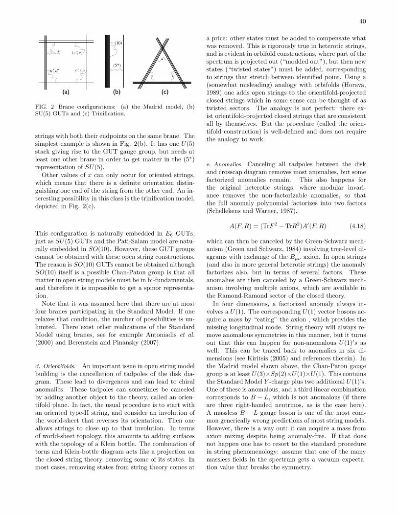
40

e+, vR

(e, )(u, d)

u, d

(10)

(5*)

Monday, 17 September 2012Monday, 17 September 2012

(a) (b) (c)

FIG. 2 Brane configurations: (a) the Madrid model, (b)SU(5) GUTs and (c) Trinification.

strings with both their endpoints on the same brane. Thesimplest example is shown in Fig. 2(b). It has one U(5)stack giving rise to the GUT gauge group, but needs atleast one other brane in order to get matter in the (5∗)representation of SU(5).

Other values of x can only occur for oriented strings,which means that there is a definite orientation distin-guishing one end of the string from the other end. An in-teresting possibility in this class is the trinification model,depicted in Fig. 2(c).

This configuration is naturally embedded in E6 GUTs,just as SU(5) GUTs and the Pati-Salam model are natu-rally embedded in SO(10). However, these GUT groupscannot be obtained with these open string constructions.The reason is SO(10) GUTs cannot be obtained althoughSO(10) itself is a possible Chan-Paton group is that allmatter in open string models must be in bi-fundamentals,and therefore it is impossible to get a spinor representa-tion.

Note that it was assumed here that there are at mostfour branes participating in the Standard Model. If onerelaxes that condition, the number of possibilities is un-limited. There exist other realizations of the StandardModel using branes, see for example Antoniadis et al.(2000) and Berenstein and Pinansky (2007).

d. Orientifolds. An important issue in open string modelbuilding is the cancellation of tadpoles of the disk dia-gram. These lead to divergences and can lead to chiralanomalies. These tadpoles can sometimes be canceledby adding another object to the theory, called an orien-tifold plane. In fact, the usual procedure is to start withan oriented type-II string, and consider an involution ofthe world-sheet that reverses its orientation. Then oneallows strings to close up to that involution. In termsof world-sheet topology, this amounts to adding surfaceswith the topology of a Klein bottle. The combination oftorus and Klein-bottle diagram acts like a projection onthe closed string theory, removing some of its states. Inmost cases, removing states from string theory comes at

a price: other states must be added to compensate whatwas removed. This is rigorously true in heterotic strings,and is evident in orbifold constructions, where part of thespectrum is projected out (“modded out”), but then newstates (“twisted states”) must be added, correspondingto strings that stretch between identified point. Using a(somewhat misleading) analogy with orbifolds (Horava,1989) one adds open strings to the orientifold-projectedclosed strings which in some sense can be thought of astwisted sectors. The analogy is not perfect: there ex-ist orientifold-projected closed strings that are consistentall by themselves. But the procedure (called the orien-tifold construction) is well-defined and does not requirethe analogy to work.

e. Anomalies Canceling all tadpoles between the diskand crosscap diagram removes most anomalies, but somefactorized anomalies remain. This also happens forthe original heterotic strings, where modular invari-ance removes the non-factorizable anomalies, so thatthe full anomaly polynomial factorizes into two factors(Schellekens and Warner, 1987),

A(F,R) = (TrF 2 − TrR2)A′(F,R) (4.18)

which can then be canceled by the Green-Schwarz mech-anism (Green and Schwarz, 1984) involving tree-level di-agrams with exchange of the Bµν axion. In open strings(and also in more general heterotic strings) the anomalyfactorizes also, but in terms of several factors. Theseanomalies are then canceled by a Green-Schwarz mech-anism involving multiple axions, which are available inthe Ramond-Ramond sector of the closed theory.

In four dimensions, a factorized anomaly always in-volves a U(1). The corresponding U(1) vector bosons ac-quire a mass by “eating” the axion , which provides themissing longitudinal mode. String theory will always re-move anomalous symmetries in this manner, but it turnsout that this can happen for non-anomalous U(1)′s aswell. This can be traced back to anomalies in six di-mensions (see Kiritsis (2005) and references therein). Inthe Madrid model shown above, the Chan-Paton gaugegroup is at least U(3)×Sp(2)×U(1)×U(1). This containsthe Standard Model Y -charge plus two additional U(1)’s.One of these is anomalous, and a third linear combinationcorresponds to B − L, which is not anomalous (if thereare three right-handed neutrinos, as is the case here).A massless B − L gauge boson is one of the most com-mon generically wrong predictions of most string models.However, there is a way out: it can acquire a mass fromaxion mixing despite being anomaly-free. If that doesnot happen one has to resort to the standard procedurein string phenomenology: assume that one of the manymassless fields in the spectrum gets a vacuum expecta-tion value that breaks the symmetry.

41

f. Boundary RCFT constructions. Just as in the heteroticstring, one can construct spectra using purely geometricmethods, orbifold methods or world-sheet constructions.Most work in the literature uses the second approach.

World-sheet approaches use boundary CFT: confor-mal field theory on surfaces with boundaries and cross-caps. This requires an extension of the closed stringHilbert space with “states” (in fact not normalizable,and hence not in the closed string Hilbert space) that de-scribe closed strings near a boundary, or in the presenceof orientation reversal. An extensive formalism for com-puting boundary and crosscap states in (rational) CFTwas developed in the last decade of last century, startingwith work by Cardy (1989), developed further by sev-eral groups, including Bianchi and Sagnotti (1990); Pra-disi et al. (1996); Fuchs and Schweigert (1998); Behrendet al. (2000); and Huiszoon et al. (1999), culminating ina simple and general formula (Fuchs et al., 2000). For anextensive review of this field see Angelantonj and Sag-notti (2002). This was applied by Dijkstra et al. (2005)to orientifolds of Gepner models, and led to a huge (of or-der 200.000) number of distinct string spectra that matchthe chiral Standard Model. This set provides an exten-sive scan over the orientifold landscape.

These spectra are exact in perturbative string theoryand not only the massless but also all massive states areknown explicitly. There are no chiral exotics, but in gen-eral there are large numbers of the ubiquitous vector-likestates that plague almost all exact string spectra. Alltadpoles are canceled, but in most cases this requireshidden sectors. However, there are a few cases whereall tadpoles cancel entirely among the Standard Modelbranes (hence no hidden sector is present) and further-more the superfluous B−L vector bosons acquires a massfrom axion mixing. These spectra have a gauge groupwhich is exactly SU(3)× SU(2)× U(1) (there are a fewadditional vector bosons from the closed sector, but theperturbative spectrum contains no matter that is chargedunder these bosons; this is the same as in the type IIAstring, which contains a vector boson that only couplesto non-perturbative states, D0-branes).

g. Results Orientifold model building has been very ac-tively pursued during the first decade of this century. Itis impossible to review all the different approaches andtheir successes and failures here, but fortunately an ex-tensive review is available (Blumenhagen et al., 2005a).The original work proposing the Madrid model (Ibanezet al., 2001) also found non-supersymmetric examples,but since only RR tadpoles were canceled and not NS-NS tadpoles, these were not stable. The search for sta-ble, supersymmetric examples took some time but wasfinally successful (Cvetic et al., 2001) although initiallythe spectra were plagued by the presence of chiral (butnon-anomalous) exotic matter.

12. Decoupling Limits

Brane model building led to an interesting change instrategy. Whereas string theory constructions were orig-inally “top-down” (one constructs a string theory andthen compares with the Standard Model), using branesone can to some extent work in the opposite direction,“bottom-up”. The idea is to start with the StandardModel and construct a brane configuration to match it,using branes localized at (orbifold) singularities. Thenthis brane configuration may be embedded in string the-ory at a later stage. This point of view was pioneered byAldazabal et al. (2000). This is a useful approach in openstring models because the gauge fields are localized onD-branes. This makes it possible to decouple gravity bysending the compactification radius to infinity. By con-trast, in heterotic string models both gravity and gaugeinteractions originate from closed string exchange, andsuch a decoupling limit would not make sense. Exampleswith Z3 singularities were given by the aforementionedauthors. Berenstein et al. (2002) considered the discretegroup ∆27, and Verlinde and Wijnholt (2007) used D3-branes on a del Pezzo 8 singularity.

The other extreme is to take the details of the StandardModel for granted and focus on issues like moduli, super-symmetry breaking and hierarchies. In this case one hasto assume that once the latter are solved, the StandardModel can be added. Both points of view are to some ex-tent a return to the “old days” of quantum field theory.On the one hand, the techniques of branes and higherdimensions are used to enrich old ideas in GUT modelbuilding; on the other hand, string theory is treated as a“framework”, analogous to quantum field theory, wheregauge groups, representations and couplings are inputrather than output.

Decoupling of gravity is an important element in recentwork on F-theory GUTs (Beasley et al., 2009a,b; Don-agi and Wijnholt, 2011b) obtained by compactifying F-theory on elliptically fibered Calabi-Yau fourfolds. Thisallows the construction of models that may be thought ofas non-perturbative realizations of the orientifold SU(5)GUT models depicted in Fig. 2(b), solving some of theirproblems, especially absence of the top-Yukawa coupling,which is perturbatively forbidden. This has led to a re-vival of Grand Unified Theories, invigorated with fea-tures of higher dimensional theories. We will returnto this in sections V.A.4 and V.B.5. See reviews byHeckman (2010); Leontaris (2011); Maharana and Palti(2013); and Weigand (2010) for further details.

An example in the second category is recent work inthe area of M-theory compactifications (Acharya et al.,2012). Getting chiral N=1 supersymmetric spectra in M-theory requires compactification on a seven dimensionalmanifold with G2 holonomy (Acharya and Witten, 2001),also known as a Joyce manifold. Much less is knownabout M-theory than about string theory, and much less

42

is known about Joyce manifolds than about Calabi-Yaumanifolds, since the powerful tool of complex geometryis not available. For this reason the Standard Model istreated as input rather than output, in the spirit of QFT.

Another kind of compactification that allows splittingthe problem into decoupled parts is the LARGE VolumeScenario (Balasubramanian et al., 2005), originally in-vented for the purpose of moduli stabilization (see sectionIV.H.1). Here both kinds of decoupling limits have beendiscussed, and there have also been steps towards puttingboth parts together (Conlon et al., 2009). This illustratesthat focusing on decoupling limits does not mean that theoriginal goal of a complete theory is forgotten. Indeed,there also exist global F-theory constructions (Blumen-hagen et al., 2010; Marsano et al., 2013).

G. Non-supersymmetric strings

Although the vast majority of the literature on stringconstructions concerns space-time supersymmetric spec-tra, in world-sheet based methods – free bosons andfermions, Gepner models, and certain orbifolds – it is aseasy to construct non-supersymmetric ones. In fact, itis easier, because space-time supersymmetry is an addi-tional constraint. These spectra are generally plagued bytachyons, but by systematic searches one can find exam-ples where no tachyons occur. This was first done in tendimensions by Alvarez-Gaume et al. (1986) and Dixonand Harvey (1986). These authors found a heteroticstring theory with a SO(16)× SO(16) gauge group, theonly tachyon-free non-supersymmetric theory in ten di-mensions, out of a total of seven. Four-dimensional non-supersymmetric strings were already constructed shortlythereafter (Kawai et al., 1986a; Lerche et al., 1987). Allof these examples employ off-diagonal left-right pairingsof partition functions. In the absence of space-time su-persymmetry, tachyonic character exist, but they may bepaired with a non-tachyonic one so that there is no phys-ical tachyon. The result can be interpreted by means of“mis-aligned supersymmetry” (Dienes, 1994). Finitenessof the vacuum energy at one-loop is due to alternatingboson and fermion surpluses at subsequent levels.

In orientifold models there are two additional ways toremove the closed string tachyons. They may also be pro-jected out by the Klein-bottle diagram (Sagnotti, 1995),or it is possible to consider supersymmetric closed stringtheories with supersymmetry broken only in the opensector. An ten-dimensional example of the latter kindwas described by Sugimoto (1999), and this is knownin general as “Brane Supersymmetry Breaking” (Anto-niadis et al., 1999).

After adding open strings one also has to worry alsoabout tachyons in the open sector. These may be avoidedby judicious choices of Chan-Paton multiplicities. Inaddition, one has to make sure that the crosscap and

disk tadpoles cancel, which implies an additional con-straint on these choices. Examples satisfying all theseconstraints were found using orbifold methods by Ange-lantonj (1998) (see also Angelantonj and Sagnotti (2002)for further references) and using Gepner orientifolds byGato-Rivera and Schellekens (2009). The latter authorseven tried to obtain the chiral Standard Model spectrumin this manner, but without success, presumably just be-cause the sample size was too small.

Non-supersymmetric strings can have a vacuum energyΛ of either sign. See for example Dienes (2006) for adistribution of values of the vacuum energy for a class ofheterotic strings. There also exist examples where Λ van-ishes exactly to all orders in perturbation theory (Kachruet al., 1999) but probably this feature does not hold be-yond perturbation theory (Harvey, 1999).

One might think that in the absence of any evidencefor low energy supersymmetry, and because of the ev-idence in favor of an accelerated expansion of the uni-verse, non-supersymmetric strings with a positive cos-mological constant are a better candidate for describingour universe than the much more frequently studied su-persymmetric ones. But the absence of supersymmetryis a serious threat for the stability of these theories, evenin the absence of tachyons in the perturbative spectrum.All of these theories have massless particles, which in-clude at least the dilaton, and usually many others. Ab-sence of tachyons only says something about the secondorder terms in scalar potentials. Higher order terms canstill destabilize these theories. In many cases there aretachyons in spectra continuously connected to them. InGinsparg and Vafa (1987) and Nair et al. (1987) this wasanalyzed for the O(16) × O(16) string, where the con-tinuous parameters were obtained by compactification ofone dimension. The (meta)-stability of brane supersym-metry breaking is discussed by Angelantonj and Dudas(2007).

There is always a dilaton tadpole. This signals that theflat background space-time that was used is not a solu-tion to the equations of motion; instead one must use deSitter (dS) or Anti-de Sitter (AdS) space with preciselythe value Λ as its cosmological constant (Fischler andSusskind, 1986a,b). Unfortunately this argument onlyprovides an explanation for the presence of the tadpole,but does not provide an exact (A)dS solution.

H. The String Theory Landscape

From the huge amount of work described in the previ-ous chapter we have learned that string theory can de-scribe all gross features of a supersymmetrized version ofthe Standard Model. But there are still some major (andmany minor) obstacles: supersymmetry must be broken,all moduli must be stabilized, a cosmological constantmust be generated, and that constant must be absurdly

43

small and positive.All of these requirements are needed for phenomeno-

logical reasons, but they also have anthropic implications.If that were not the case, we should already ask ourselveswhy string theory, to first approximation, tends to pre-dict all of these features so catastrophically wrong.

It is possible that the supersymmetric vacua we areable to discuss are merely an irrelevant corner in a huge,predominantly non-supersymmetric landscape. Thiswould mean that our current view is completely dis-torted by our technical limitations. This may be true,but it is not a useful working hypothesis. The exact non-supersymmetric string theories discussed above illustratethis point: it has been very hard to to make progress inthis area of string theory.

Fortunately there does exist a plausible anthropic argu-ment why the – apparently – ubiquitous supersymmetricvacua are not observed, see sec. III.B.4. With super-symmetry out of the way, the other two major prob-lems change character. It not very plausible that in anon-supersymmetric theory there would be exactly flatmoduli potentials or an exactly vanishing cosmologicalconstant. One could contemplate the possibility that welive in a universe where one or more moduli are slowlyrunning away to infinity. They would then drag vari-ous constants of nature along with them, and changingconstants of nature evidently create anthropic problems.This will be discussed in section V.E. It seems howevermore plausible that we need to find stable points in thepotential.

If such stable point exist, all moduli will get masses.There are important restrictions on their masses. Ifthey are extremely small, moduli can mediate long-rangeforces that would be observed as violations of the equiva-lence principle. But since nature abhors light scalars thisis not a major worry. Any mass below the scale of super-symmetry breaking would be unnatural, so the expectedmass of the moduli is the supersymmetry breaking scale.

A crucial test for the string landscape is the existenceof (meta)stable dS vacua. They are needed for three rea-sons: there is evidence that our own universe approachessuch a space at late times, eternal inflation requires theexistence of at least one dS vacuum, and cosmic inflationin our own universe may need, at least approximately, adS space as well. Furthermore, for explanations of ap-parent anthropic tunings we need a large number of suchspaces, and they have to be distributed in the right way.

1. Existence of de Sitter Vacua

The art of constructing dS vacua is based on as-sembling the many ingredients of the string toolboxin a controlled way: branes, fluxes, orientifold planes,non-perturbative effects (usually in the concrete formsof “brane instantons” or gaugino condensation), world-

sheet perturbative corrections and string perturbativecorrections. Fortunately, several fairly recent review arti-cles are available, e.g. Grana (2006); Douglas and Kachru(2007); Blumenhagen et al. (2007b); Denef (2008) andthe slightly more accessible one by Denef et al. (2007).Here we will just give a brief summary, and mention somerecent developments.

The most explicit results have been obtained in type-IIB (and related F-theory) compactifications. One startswith a Calabi-Yau compactification. The continuous de-formations of such manifolds are described by moduliof two different kinds: h21 complex structure (“shape”)moduli and h11 Kahler (“size”) moduli, where h21 andh11 are the Hodge numbers of the CY manifold. One canadd 3-form RR and NS fluxes, 5-form fluxes, denotedF3, H3 and F5 respectively, and D3 and D7 branes.

In type-IIB theories the 3-form fluxes can stabilize allcomplex structure moduli. This stabilization is due to atree-level term in the superpotential that takes the form(Gukov et al., 2000)

Wflux =

∫(F3 − τH3) ∧ Ω , (4.19)

where τ = a + ie−φ, and a is the axion and φ the dila-ton. The dependence on the complex structure moduliis through Ω, the holomorphic three-form of the Calabi-Yau manifold. This term also fixes the dilaton and axion.However, Wflux does not depend on the Kahler moduliand hence cannot fix them. This leaves therefore at leastone modulus unfixed, since every CY manifold has atleast one Kahler modulus.

The next step is to try and fix the size moduli with non-perturbative terms in the superpotential. These take theform W ∝ exp(iλs), where s is the size modulus and λa parameter. Such terms can be generated by instantonsassociated with Euclidean D3-branes (Witten, 1996) orfrom gaugino condensation in gauge groups on wrappedD7 branes. Assuming at least one of these effects tobe present, Kachru et al. (2003b) (usually referred toas KKLT) obtained string vacua with all moduli stabi-lized. This work builds on several earlier results, such asDasgupta et al. (1999); Giddings et al. (2002); and Kle-banov and Strassler (2000) and other references cited.KKLT considered the special case h11 = 1, so that onlyone size modulus needs to be stabilized. They arguedthat by suitable choices of fluxes one can obtain solu-tions where supersymmetry is unbroken, and all world-sheet and string perturbative corrections (i.e the α′ andgs expansion) are small. The solution obtained in thisway has a negative vacuum energy, and is a fully stabi-lized supersymmetric AdS vacuum. This is achieved bychoosing fluxes so that Wflux is small, the volume is largeand the dilaton (which determines the string coupling)is stabilized at a point where the coupling is small. Here“small” and “large” refer to tunings by just a few ordersof magnitude.

44

This is however just a “scenario”, since the existenceof the non-perturbative effects still needs to be demon-strated. Many would-be instantons do not contribute be-cause of superfluous zero-modes. It turns out that mod-els with just one Kahler modulus do not work, and thatinstanton contributions are “not generic” (Denef et al.,2004; Robbins and Sethi, 2005) but still occur sufficientlyoften to allow a huge number of solutions.

The next step is more problematic and more contro-versial. One must break supersymmetry and obtain adS vacuum (this is called “up-lifting”). In KKLT thisis done by adding an anti-D3 brane in a suitable loca-tion on the Calabi-Yau manifold, such that the validityof the approximations is not affected. Anti-D3 branesexplicitly violate supersymmetry, and hence after intro-ducing them one loses the control offered by supergravity.Of course, supersymmetry must be broken anyway, butit would be preferable to break it spontaneously ratherthan explicitly. Attempts to realize the KKLT upliftingin supergravity or string theory have failed so far (Benaet al., 2012, 2013), but opinions differ on the implica-tions of that result. There exist several alternatives toD3-brane uplifting (see e.g. Burgess et al. (2003); Salt-man and Silverstein (2004); Lebedev et al. (2006); andalso Covi et al. (2008) and Westphal (2008) for furtherreferences.)

The result of a fully realized KKLT construction is astring vacuum that is free of tachyons, but one still has toworry about non-perturbative instability. The uplift con-tribution vanishes in the limit of large moduli, so thereis always a supersymmetric vacuum in that limit, sepa-rated from the dS vacuum by the uplifted barrier thatstabilized the AdS vacuum. One can work out the tun-neling amplitude, and KKLT showed that it is genericallymuch larger than the observed lifetime of our universe,yet well below the theoretical upper limit in dS space,the Poincare recurrence time. See also Westphal (2008)for a systematic analysis of several kinds of minima.

An alternative scenario was described by Balasubra-manian et al. (2005). The starting point is the same:type-IIB fluxes stabilizing the complex structure mod-uli and the dilaton and axion. But these authors useα′ corrections to their advantage rather than tuning pa-rameters to minimize them. By means of suitable (α′)3

corrections they were able to find minima where all mod-uli are stabilized at exponentially large volumes in non-supersymmetric AdS vacua. The fact that α′ correc-tions can be important at large volumes may be counter-intuitive, but can be understood in terms of the no-scale structure of the underlying supergravity. For otherwork discussing the importance of perturbative correc-tions see Becker et al. (2002); Berg et al. (2006); Bobkov(2005); and von Gersdorff and Hebecker (2005). Addi-tional mechanisms are then needed to lift the vacuum todS.Aan explicit example was presented recently by Louiset al. (2012). This scenario requires special Calabi-Yau

manifolds with h21 > h11 > 1 and a structure consistingof one large topological cycle and one or more small ones.This has been given the suggestive name “Swiss Cheesemanifold”. Not every Calabi-Yau manifold has this prop-erty, but several hundreds are known (Cicoli et al., 2012b;Gray et al., 2012). A natural hierarchy can be obtainedby associating Standard Model branes with the small cy-cles. This is called the LARGE volume scenario (LVS).

Although type-IIA and type-IIB string theories in tendimensions only differ by a single sign flip, the discussionof moduli stabilization for the compactified theories isvastly different. This is because in type-IIA theories theavailable RR-fluxes are even-forms, and the available D-branes are D-even branes. Since there still are three formNS-fluxes one now gets flux potentials that depend on thecomplex structure moduli and others that depend on theKahler moduli. As a result, all moduli can now be stabi-lized classically by flux potentials (DeWolfe et al., 2005)(see however McOrist and Sethi (2012)). Unfortunately,it can also be shown (Hertzberg et al., 2007) that none ofthe aforementioned ingredients can be used to lift thesetheories to dS. There are more ingredients available, butso far no explicit examples are known (see Danielssonet al. (2011) for a recent attempt).

Moduli stabilization for heterotic M-theory was dis-cussed by Braun and Ovrut (2006). Supersymmetry isbroken and a lift to dS achieved using heterotic five-branes and anti-five-branes. For the perturbative het-erotic strings in the “mini-landscape” a scenario for mod-uli stabilization was presented by Dundee et al. (2010).Acharya et al. (2006) discussed this for M-theory com-pactifications on manifolds with G2 holonomy. Theseauthors do not use fluxes, because in this class of mod-els they would destroy the hierarchy. Instead, all moduliare stabilized by non-perturbative contributions gener-ated by strong gauge dynamics. To this end they in-troduce two “hidden sector” gauge groups. A similarmechanism was applied to type-IIB theories by Bobkovet al. (2010). These arguments often rely on plausiblebut unproven assumptions about terms in potentials andnon-perturbative effects. In explicit models the requiredterms may be absent, even though generically allowed.

2. Counting and Distributions

Fluxes are characterized by integers specifying how of-ten they wrap the topological cycles on the manifold.However, the total number of possibilities is limited byconditions for cancellation of tadpoles. For a large classof F-theory constructions this condition takes the form

ND3 −ND3 +1

2π4α′2

∫H3 ∧ F3 =

χ(X)

24, (4.20)

where the first two terms denote the net contributionfrom D3-branes, the third one the contribution due to

45

fluxes and the right hand side is a contribution (“tadpolecharge”) from orientifold planes (Sethi et al., 1996); χ(X)is the Euler number of a Calabi-Yau fourfold defining theF-theory under consideration. Since the flux contributionis always positive this makes the number of possibilitiesfinite.

This has been the starting point for estimates of thetotal number of flux vacua. Douglas (2004a) gave thefollowing estimate (based on Ashok and Douglas (2004)and Denef and Douglas (2004))

Nvac ≈(2πL)K/2

(K/2)!, (4.21)

where L is the aforementioned tadpole charge and K thenumber of distinct fluxes. For typical manifolds this givesnumbers of order 10N , where N is of order a few hun-dred. This is the origin of the (in)famous estimate 10500.Note that Eq. (4.21) should still be summed over dis-tinct manifolds, that it only counts fluxes and no othergadgets from the string theory toolbox, and that none ofthese 10500 vacua includes the Standard Model, becauseno structure (like intersecting D-branes or singularities)is taken into account to produce chiral matter. Indeed,the presence of chiral matter may influence moduli sta-bilization in a negative way (Blumenhagen et al., 2008).

It is noteworthy that this formula turns a nuisance (alarge number of moduli) into a virtue: the large numberof moduli gives rise to the exponent of Eq. (4.21), andit is this large exponent that makes neutralization of thecosmological constant possible. This is not automaticallytrue for all string compactifications and moduli stabiliza-tion mechanisms; the existence of a sufficiently large setof vacua has to be demonstrated in each case. Bobkov(2009) has shown that fluxless G2 compactifications ofM-theory also yield a large discretuum of vacua.

In type-IIA constructions there are also tadpole con-ditions to satisfy, but in this case they do not reduce thevacuum count to a finite number. Instead it was foundthat supersymmetric AdS vacua exist at arbitrarily largevolume, in combination with an arbitrarily small cosmo-logical constant. This implies that the total number ofvacua is infinite, but it can be made finite by makinga phenomenologically inspired cut on the volume of thecompactification. Acharya and Douglas (2006) presentedgeneral arguments suggesting that the number of stringvacua must be finite, if one puts upper bounds on thecosmological constant and the compactification volume.

The most important contribution not taken into ac-count in Eq. (4.21) is the effect of supersymmetry break-ing. These computations count supersymmetric AdSvacua. They must still be lifted to dS by a supersym-metry breaking contribution. Already in Douglas (2004a)the possibility was mentioned that most of the AdS vacuamight become tachyonic if such a lift is applied. Recentwork seems to indicate that this is indeed what happens.In Chen et al. (2012b) this was investigated for type-IIA

vacua and in Marsh et al. (2012a) for supergravity. Theseauthors analyze general scalar potentials using randommatrices to determine the likelihood that the full massmatrix is positive definite. They find that this is expo-nentially suppressed by a factor ≈ exp(−cNp), where Nis the number of complex scalar fields and p is estimatedto lie in the range 1.3 to 2. This suppression can be re-duced if a large subset of the scalars is decoupled by giv-ing them large supersymmetric masses. Then only thenumber of light scalars contributes to the suppression.Even more worrisome results were reported recently byGreene et al. (2013). In a study of landscapes modeledwith scalar fields, they found a doubly exponential de-crease of the number of meta-stable vacua as a functionof the number of moduli, due to dramatic increases intunneling rates.

3. Is there a String Theory Landscape?

It is generally accepted that there exists a large land-scape of fully stabilized supersymmetric AdS solutions.But these do not describe our universe. Not in the firstplace because of the observation of accelerated expansionof the universe, but because of the much more establishedfact that our vacuum is not supersymmetric. Supersym-metric vacua have a vacuum energy that is bounded fromabove at zero. Supersymmetry breaking makes positivecontributions to vacuum energy. Hence if stable non-supersymmetric vacua exist (which few people doubt), itwould be highly surprising if their vacuum energy couldnot surpass the value zero. Most arguments for or againstthe existence of dS vacua do not really depend on the signof the cosmological constant; +10−120 is nearly indistin-guishable from −10−120. Hence one would expect dis-tributions to behave smoothly near zero, although theymay drop off rapidly.

By now there are many constructions of dS vacua, al-though there are always some assumptions, and it is of-ten not possible to check the effect of higher order world-sheet or string loop corrections. But given the large num-ber of possibilities, it would require a miracle for all ofthem to fail. If that is the case there should exist somegeneral no-go theorem that was overlooked so far.

But the mere existence of vacua with positive Λ is notenough. To make use of the Bousso-Polchinski neutral-ization of Λ a sufficiently dense discretuum of such vacuais needed. This mechanism relies on the fact that what-ever the contribution of particle physics, cosmology andfundamental theory is, it can always be canceled to 120significant digits by flux contributions, without makingactual computations with that precision. If in reality thesedistributions are severely depleted in part of the range, orhave a highly complicated non-flat structure, this argu-ment would fail. There might still exist a huge landscape,but it would be useless.

46

The mighty landscape of a decade ago has been erod-ing at an alarming rate. The actual number of vacuais the product of huge numbers divided by huge sup-pression factors. Perhaps this will re-ignite dreams of aunique theory. Could it be that the product is exactlyone, with the Standard Model and the observed cosmo-logical constant as the only survivor? That would be anabsurd example of the second gedanken computation ofsection III.C. Any hopes that landscape erosion will re-duce the number of de Sitter vacua to one are unfounded,but there is a risk that it will be reduced to zero.

More fundamental objections against the use of effec-tive potentials in quantum gravity or the formulation ofQFT and string theory in de Sitter space have been raisedby Banks (2012). If these objections are valid, we maynot have any theoretical methods at our disposal to dealwith the apparent accelerated expansion of the universe.

V. THE STANDARD MODEL IN THE LANDSCAPE

In this chapter we will discuss how the main features ofthe Standard Model fit in the String Theory Landscape,taking into account anthropic restrictions and analyticaland numerical work on landscape distributions.

It would be interesting to know if there are any quan-tum field theories that do not have a place somewhere inthe string landscape. For a discrete, non-supersymmetriclandscape, obviously a continuous infinity of quantumfield theories is not realized in any vacuum, but one canphrase this question in a meaningful way for supersym-metric theories. In (Vafa, 2005) it was argued that in-deed such a “swampland” of non-realizable quantum fieldtheories indeed exists, one of the examples being the ten-dimensional anomaly free U(1)496 N = 1 gauge theory.Further evidence is provided in (Fiol, 2010). Perhapsthere is no swampland for supersymmetric theories insix dimensions, but this could be due to the much morepowerful chiral anomaly constraints (Kumar and Taylor,2011). In four dimensions this issue remains unsettled.

A. The Gauge Sector

It is by now abundantly clear that string theory canreproduce the discrete structure of the Standard Model:the gauge group and chiral fermion representations. Wecannot even begin to enumerate all the papers that suc-ceeded in doing this.

1. Gauge Group and Family Structure

a. Why SU(3) × SU(2) ×U(1)? From the landscape per-spective, one might hope that the gauge group can be un-derstood using string theory plus anthropic constraints.The anthropic constraints are hard to determine, but all

three factors of the gauge group are needed for our kindof life. Electromagnetism is so essential that it is im-possible to imagine life without it. One can imagine lifewithout SU(3)color and only electromagnetism, but it isby no means obvious that such universes will really cometo life. The weak interactions also play a crucial role inour universe, but perhaps not in every habitable one (seesection III.B.4).

The choice of fermion representation is also essential,but it is even harder to determine what happens if wechange it. It is possible that it is chiral in order to keepthe fermions light (a plausible reason why SU(2)weak

might be needed). Chiral fermions have chiral anoma-lies that must be canceled. This fixes to some extentthe particle content of a single quark and lepton family,if one insists on simplicity. See Shrock (2008) for somegedanken variations of the representations in a family.

If life requires electromagnetism, a non-abelian stronginteraction group, and a chiral spectrum that becomesnon-chiral after symmetry breaking at energies far be-low the Planck scale, perhaps the one-family StandardModel is the simplest option one can write down. Morecomplicated possibilities are easy to find. For example,changing the number of colors from 3 to some odd in-teger N and the quark charges to p/N for suitable p,one can find an infinite series of cousins of the StandardModel (Shrock, 1996) that, for all we know, are anthropi-cally equally valid. It is likely that in the landscape smallgroups are statistically favored: then N = 3 would be thefirst acceptable value. If furthermore small numbers ofgauge group factors are also favored, our Standard Modelmight be the statistically dominant anthropic choice.

It has also been suggested that the choice N = 3 forthe number of colors (with everything else kept fixed) isa consequence of the fact that only for N = 3 there isa simple GUT embedding (Shrock, 2007). This expla-nation would require the landscape to be dominated byGUT gauge groups.

b. Landscape scans of groups and representations. Therehave been several studies of distributions of groups andrepresentations in sub-landscapes, but because of lackof a sufficiently well-defined question there is no goodanswer either. For free fermion constructions of heteroticstrings see e.g Dienes (2006); Dienes et al. (2007); Renneret al. (2011, 2012).

In Blumenhagen et al. (2005b) this was done for orien-tifold models. Kumar and Wells (2005) derived a formulaof the average gauge group rank (for D3-brane gaugegroups of type-IIB flux vacua). Anastasopoulos et al.(2006) gave a classification of all brane models with atmost four brane stacks that contain the Standard Model,and a scan for realizations of these options in Gepnerorientifolds was presented. For other work on distribu-tions of gauge group features see Balasubramanian et al.

47

(2010) and Kumar (2006). An important caveat is thatall of these studies are done on exact realizations in spe-cial points in moduli space. This is therefore not truelandscape “statistics”. One would really like to see dis-tributions of physical quantities for fully stabilized dSvacua, but this is not technically possible at present.These studies are also plagued by over-counting prob-lems. Only some features of a spectrum are sampled,and one cannot be certain if two identical spectra stilldiffer in some other respect. For this reason, comparingtotal numbers of “vacua” between different approaches ismeaningless. Drawing conclusions is also made difficultbecause of limited sampling (Dienes and Lennek, 2007,2009).

2. The Number of Families

a. Why three families? We are made out of just one fam-ily of fermions. There are no good arguments why threefamilies should be anthropically required, although someunconvincing arguments can be pondered, based on therole of the s quark in QCD, of the muon in biologicalmutations, the top quark in weak symmetry breaking, orthe CP-violating CKM angle in baryogenesis. See alsoSchellekens (2008) and Gould (2010) for arguments andcounter-arguments.

Perhaps one day we will discover a good anthropic rea-son for three families. If not, the number of families wasjust picked out of a distribution. Multiple families area generic feature in string theory, due to to topologicalquantities like Hodge numbers of compactification man-ifolds or intersection numbers of branes (although oftenthis notion is muddled by attempts to distinguish familiesin order to explain mass hierarchies).

b. Landscape scans of the number of families. Landscapestudies of the number of families tend to suffer from lamp-post artifacts: initial studies of simple models favor mul-tiples of four or six families and disfavor three, but asmore general models are studied the number three be-comes less and less challenged.

The number of families was studied first in the contextof heterotic Calabi-Yau compactifications (with SU(3)spin connection embedded in E8) and their CFT real-izations, especially Gepner models and orbifolds, wherethe number of families is half the Euler number of themanifold. Systematic studies of Gepner compactifica-tions with E6 and SO(10) gauge groups were presentedby Fuchs et al. (1990) and Schellekens and Yankielowicz(1990). In all but one exceptional case4 (Gepner, 1987),

4 This Gepner model is closely related the first three-family Calabi-Yau manifold, see (Schimmrigk, 1987).

the number of families is a multiple of six or – less often–four. Gato-Rivera and Schellekens (2010) enlarged thescope by allowing broken GUT groups and asymmetricrealizations of space-time and world-sheet supersymme-try (which are not required in the bosonic sector of theheterotic string, but automatically imposed in symmetricconstructions). This did not lead to additional cases ofthree-family models. The reason why the number threewas so hard to get has never been understood, but theproblem disappears in more general constructions. Forexample, a much larger scan of Euler numbers of classesof Calabi-Yau manifolds (Kreuzer and Skarke, 2002) doesnot show a strong suppression of Euler number six. Fur-thermore, in Gepner constructions the problem disap-pears if one uses different building blocks for the left-and the right-moving sector. Modular invariance makesthis hard to do, but matching building blocks which areisomorphic (in the sense of the modular group) but notidentical can be constructed, and lead to family distribu-tions that are peaked at zero (which is anthropically ex-cluded) and fall of slowly (Gato-Rivera and Schellekens,2011a,b) In these distributions, three families are aboutas common as one, two and four, but numbers larger thansix occur only rarely. This behavior persists in the moregeneral class of orbifold permutations of Gepner models(Maio and Schellekens, 2011).

A similar conclusion can be drawn for free-fermionicconstructions of heterotic strings. Here modular invari-ance can be solved in general, and hence this approachdoes not suffer from a bias towards symmetric construc-tions, as do the Gepner models. However, it should bekept in mind that most scan done in this context are bi-ased towards three families because a special choice offermion boundary conditions, the so-called NAHE set(Antoniadis et al., 1989) is used, a priori designed toproduce three families. It has been suggested that inthis context the number of families can be understood as“(10-4)/2”, i.e. half the number of compactified dimen-sions (Faraggi et al., 2004), but in a systematic scan ofthis class (Faraggi et al., 2007) a distribution was foundthat is peaked around zero, and with three families oc-curring in about 15% of all cases.

In most other constructions only three family spectrahave been studied, so that we cannot be certain how spe-cial they are. In the “heterotic mini-landscape”, see e.g.Lebedev et al. (2007, 2008b), the requirement of havingthee families reduces the sample size by more than anorder of magnitude. This is in rough agreement with theforegoing results.

In orientifold models the family distribution also peaksat zero, but falls off more rapidly. In a study of Gep-ner orientifolds with Standard Model gauge groups (Dijk-stra et al., 2005) the number of three family spectra wasabout two orders of magnitude less than those with twofamilies. Qualitatively similar results were obtained forT 6/Z2 × Z2 orientifolds by Gmeiner et al. (2006). These

48

authors found a large dip in the distribution preciselyfor three families. However, a more detailed analysis ofthe same class (Rosenhaus and Taylor, 2009) does notshow such a dip. These authors found most spectra inthe tail of the distribution at large moduli, not consid-ered in (Gmeiner et al., 2006) (however, they also foundthat in this tail there is a huge suppression due to K-theory constraints, which was estimated, but not fullytaken into account). A general analysis of brane inter-section numbers (giving rise to chiral fermions) for thisclass, using both analytical and numerical methods, waspresented by Douglas and Taylor (2007). These conclu-sions depend strongly on the kind of orbifold considered.For example, Gmeiner and Honecker (2008) found largenumbers of three family models for T 6/Z ′6 orientifolds(the prime indicates a certain action of Z6 on the torusT 6. On the other hand, in an extensive study of freefermion orientifolds, no three family models were found((Kiritsis et al., 2009)).

Taking all these results together one may conclude thatgetting three families may be slightly more difficult thangetting one or two, but it is at worst a landscape natu-ralness problem at the level of a few percent, and eventhis suppression may be due to the examples being toospecial. Therefore it is legitimate at this point to viewthe number of families simply as a number that came outof a distribution, which requires no further explanation.

3. Grand Unification in String Theory

a. Fractional Charges. A remarkable feature of the quarkand lepton families is the absence of fractional electriccharges for color singlets. There is no evidence that freefractionally charged particles exist in nature, with a limitof less than 10−20 in matter (Perl et al., 2009), undercertain assumptions about their charges. If indeed thereare none, the global Standard Model gauge group is notSU(3)× SU(2)×U(1), but S(U(3)×U(2)). The reasonis that the former allows representations with any realvalues for the U(1) charge, whereas in the latter case thecharges are restricted by the rule

t33

+t22

+1

6= 0 mod 1, (5.1)

where t3 is the triality of the SU(3) representation andt2 the duality of SU(2), twice the spin modulo inte-gers. This relation implies integral charges for color-singlet states. But this is just an empirical rule. Nothingwe know at present imposes such a relation. Anomalycancellation restricts the allowed charges, but arbitrarycharges, even irrational ones, can be added in non-chiralpairs or as scalar fields. In fundamental theories one mayexpect charges to come out quantized (due to Dirac quan-tization for magnetic monopoles), but that still does notimply that they are quantized in the correct way.

Already for almost four decades we know an excellentexplanation for the empirical fact (5.1): Grand Unifica-tion, which embeds the Standard Model in a single, sim-ple gauge group SU(5) (Georgi and Glashow, 1974). Sofar this idea remains just a theory. In its simplest formit made a falsifiable prediction, the decay of the proton,and this was indeed falsified. It also predicts magneticmonopoles, but these are too heavy to produce in acceler-ators, and any primordial ones would have been dilutedby inflation. Despite the falsification, the basic idea isstill alive, because it is not hard to complicate the theory(for example by making it supersymmetric) and avoidthe falsification. Low energy supersymmetry lifts the ex-pected proton life time from 1030 years to 1036 years,just outside the range of current experiments (there areother potential sources of proton decay in supersymmet-ric theories, which must be carefully avoided). The ideaof group-theoretic unification is too compelling to giveup on, but to strengthen the argument we must convinceourselves that the absence of fractional charges in ouruniverse could not have an anthropic origin.

It is obvious that the existence of fractionally chargedparticles with suitable chosen masses and abundancescan be potentially catastrophic. For example, the elec-tron might decay into two or more lighter half-integralcharges. But then one would still have to rule out atomsusing some of these particles instead of electrons. Obvi-ously the lightest fractionally charged particle would bestable, and this would seriously frustrate chemistry, stel-lar dynamics and big bang nucleosynthesis. But it is hardto see how one can turn this into an anthropic argumentagainst any such particle, regardless of mass, abundance,and charge.

Hence we must conclude that the structure of the Stan-dard Model gauge group strongly suggests an embeddingin SU(5) or a larger group, at a more fundamental level.For a while it seemed reasonable that one day a new,more symmetric theory would be found with a built-inGUT structure.

Indeed, if Grand Unification is a fundamental law ofphysics, one might hope to find a theory that unequivo-cally predicts it. But string theory is not that theory. Itseemed like that for a while in 1984, when GUTs cameout “naturally” from Calabi-Yau compactifications of theE8 × E8 heterotic string, but within a few years it be-came clear that GUTs are by no means the only possibleoutcome, and that furthermore the GUTs obtained fromCalabi-Yau related compactifications do not genericallybreak in the correct way to the Standard Model gaugegroup. Let us first understand why GUT gauge groupscome out so easily.

b. Heterotic Strings. There are two equivalent ways ofunderstanding why Grand Unification emerges so easilyin E8 × E8 heterotic strings. In Calabi-Yau compact-

49

ification this comes from the embedding of the SU(3)holonomy group of the manifold in one of the E8 fac-tors, breaking it to E6, an acceptable but not ideal GUTgroup. In world-sheet constructions this is a consequenceof the “bosonic string map” (Lerche et al., 1987) used tomap the fermionic (right-moving) sector of the theoryinto a bosonic one, in order to be able to combine itin a modular invariant way with the left-moving sector.The bosonic string map takes the fermionic sector of aheterotic or type-II string, and maps it to a bosonic sec-tor. The world-sheet fermions ψµ transform under theD-dimensional Lorentz group SO(D−1, 1). The bosonicstring map replaces this by an SO(D+ 6)×E8 affine Liealgebra, which manifests itself as a gauge group in space-time. In (Lerche et al., 1987) this trick was used to mapthe problem of finding modular invariants to the alreadysolved problem of characterizing even self-dual lattices.This automatically gives rise to a four-dimensional the-ory with an SO(10)×E8 gauge group and chiral fermionsin the spinor representation of the first factor.

Finding modular invariant partition functions for inter-acting CFTs is a much harder problem. But one can startwith a canonical solution, a symmetric pairing of the left-and the right-moving degrees of freedom, which is auto-matically modular invariant. Unfortunately that is notvery suitable for heterotic strings, where the right sectoris fermionic and the left sector bosonic. This is where thebosonic string map comes in. To get a modular invari-ant heterotic string one can start with a symmetric andmodular invariant type-II string, and map the fermionicsector to a bosonic sector. In the process, one obtainsan SO(D + 6) × E8 gauge symmetry for free. This wasindeed the method used in (Gepner, 1988). For D = 4this yields SO(10) (we ignore the E8), and furthermoreit is automatic that space-time fermions belong to thespinor representation of that group. This is the perfectGUT theory. The 16-dimensional spinor of SO(10) con-tains precisely one family of the Standard Model, with aright-handed neutrino.

This SO(10) group is seen by many as the ideal GUTgroup. The somewhat less ideal E6 appearing in typi-cal Calabi-Yau compactifications is an artifact of theseconstructions. This has to do with space-time super-symmetry. If one requires the spectrum to be supersym-metric in space-time, an additional is needed. This goesby many names, such as GSO-projection, β-projection,spectral flow, or adding a spinor root to the chiral alge-bra. But in any cases it implies a modification of theright, fermionic sector of the theory. This violates mod-ular invariance unless we also change the left, bosonicsector. The canonical way of doing that is by adding aspinor root to SO(10), turning it into E6. But there areother ways than the canonical one. In many cases, onecan find another operator that transforms under modu-lar transformations exactly as the spinor root, but has adifferent conformal weight (the eigenvalue of L0, which is

observed as mass). Consequently it is not visible in themassless particle spectrum, and in particular SO(10) isnot extended to E6.

Therefore the appearance of E6 in early string con-structions is probably best viewed as a “lamp-post” ef-fect. It is what happens in the most easily accessiblefully symmetric constructions, but it is not generic. Thegeneric gauge group is SO(10) with matter in the spinorrepresentation.

These SO(10) GUTs are the best hope for believ-ers in the uniqueness paradigm. There is indeed some-thing unique about it: the (16) of SO(10) is the smallestanomaly free complex irreducible representation for anyLie-algebra. But this is spoiled a little because it oc-curs three times. Still, with only slight exaggeration onecan state that this ideal GUT group emerges uniquelyfrom the heterotic string. All we had to do is specifythe space-time dimension, D = 4, and apply the bosonicstring map, and we get SO(10) for free.

But this is as good as it gets. Nothing in the struc-ture of the Standard Model comes out more convinc-ingly than this. A mechanism to break SO(10) toSU(3)×SU(2)×U(1) can be found, but it does not comeout automatically. Furthermore, it works less nicely thanin field theory GUTs. The heterotic string spectrum doesnot contain the Higgs representation used in field theory.The breaking can instead be achieved by adding back-ground fields (Wilson lines).

But in that case the full spectrum of these heteroticstrings will never satisfy (5.1), and it is precisely the deepunderlying structure of string theory that is the culprit.In a string spectrum every state is relevant, as is fairly ob-vious from the modular invariance condition. Removingone state destroys modular invariance. In this case, whatone would like to remove are the extra gauge bosons inSU(5) ⊂ SO(10) in comparison to SU(3)×SU(2)×U(1).To do this one has to add something else to the spectrum,and it turns out that the only possibility is to add some-thing that violates (5.1) and hence is fractionally charged(Schellekens, 1990). The possible presence of fractionalcharges in string spectra was first pointed out by Wenand Witten (1985) and the implications were discussedfurther in Athanasiu et al. (1988).

c. Fractional charges in Heterotic spectra. The occurrenceof fractional charges in heterotic string spectra has beenstudied systematically for free fermion constructions andfor heterotic Gepner models. All these models realizethe gauge group in the canonical heterotic way, as a sub-group of SO(10) (which may be further extended to E6).There is a total of four distinct subgroups that one mayencounter within SO(10). These subgroups are furthersubdivided into several classes, distinguished by the min-imal electric charge quantum that occurs in their spectra.These charge quanta are not determined by group the-

50

ory in quantum field theory, but by affine Lie algebrasin string theory. This gives a total of eight possibilities,with charge quanta given in curly brackets:

SU(3)× SU(2)× U(1)× U(1) 16 ,

13 ,

12

SU(3)× SU(2)L × SU(2)R × U(1) 16 ,

13

SU(4)× SU(2)L × SU(2)R 12

plus SU(5)×U(1) and SO(10), which automatically yieldinteger charges. This classification applies to all con-structions in the literature where the Standard Modelis realized with level 1 affine Lie algebras, with a stan-dard Y charge normalization, embedded via an SO(10)group. The minimal electric charge must be realized inthe spectrum, but it is in principle possible that fraction-ally charged particles are vector-like (so that they mightbecome massive under deformations of the theory), havePlanck-scale masses or are coupled to an additional in-teraction that confines them into integer charges, just asQCD does with quarks.

But how often does this happen? In (Assel et al.,2011) a large class of free fermionic theories with Pati-Salam spectra. These authors did find examples withthree families where all fractionally charged particles areat the Planck mass, but only in about 10−5 of the chiralspectra. In (Gato-Rivera and Schellekens, 2010, 2011a,b;Maio and Schellekens, 2011) a similar small fraction wasseen, but examples were only found for even numbers offamilies. These authors also compared the total numberof spectra with chiral and vector-like fractional charges,and found that about in 5% to 20% of the chiral, non-GUT spectra the fractional charges are massless, butvector-like. They also found some examples of confinedfractional charges.

If one assumes that in genuine string vacua vector-like particles will always be very massive, this is a mildlandscape naturalness problem. But avoiding fractionalcharges by chance is an unattractive solution. There maybe a better way out. In orbifold models SO(10) is bro-ken using background gauge fields on Wilson lines. Inthis process fractional charges must appear, and there-fore they must be in the twisted sector of the orbifoldmodel. If the Wilson lines correspond to freely actingdiscrete symmetries of the manifold (see (Witten, 1985)),the twisted sector fields are massive, and hence all frac-tionally charge particles are heavy. This method is com-monly used in Calabi-Yau based constructions, e.g. (An-derson et al., 2010), but is chosen for phenomenologicalreasons, and hence this does not answer the question whynature would have chosen this option. Also in the het-erotic mini-landscape an example was found (Blaszczyket al., 2010), but only after numerous examples withmassless, vector-like fractional charges. But these au-thors suggested another rationale for using freely actingsymmetries, namely that otherwise the Standard ModelY charge breaks if the orbifold singularities are “blown

up”. It is not clear how that would impact models atthe exact orbifold point without blow-up, but at least itsuggests a solution.

Another disappointment from the perspective of theuniqueness paradigm is that the natural appearanceof SO(10) is really just a lamppost effect as well.Generic heterotic strings constructed using free fermionor bosonic methods can have many other gauge groups.If SO(10) comes out, that is just by choice.

d. Higher Level Heterotic String GUTs. Within the con-text of heterotic strings there is another way of dealingwith the unification problem. It is possible to constructheterotic string theories with affine Lie algebras of levelshigher than 1. The first example was the aforementionedE8 level 2 in 10 dimensions, which is non-supersymmetricand tachyonic. In four dimension one can construct suchtheories as well ((Lewellen, 1990)) and even get GUTgauge groups ((Kakushadze and Tye, 1997)). This re-moves one problem of the level 1 GUTs, namely that thegauge group can now be broken in the standard way usedin field theory GUTs, by means of a Higgs mechanism.By emulating field theory GUTs one can reproduce theirsuccess The canonical case is the breaking of SU(5) toSU(3) × SU(2) × U(1). This requires a Higgs boson inthe adjoint representation of SU(5), and matter in thatrepresentation be massless if SU(5) is realized as a level1 affine algebra. Adjoints can only appear in the gaugeboson sector, either as gauge bosons or as gauginos, butnot in the matter sector. Allowing higher levels solvesthat problem, but at a price. Adjoint representationsare now allowed, but so are other tensor representations.The beauty of the canonical heterotic GUTs is that onlyfundamental representation of SU(3) and SU(2) are al-lowed as massless states. This is a huge improvement overquantum field theory, where there is no restriction on therepresentations. But this is partly lost if one considershigher levels. The Standard Model can be “accommo-dated”, but there is no construction where it really comesout as naturally as one might have hoped.

e. GUTs and Intersecting Brane Models. Yet another pos-sibility to get the Standard Model is by means of stacks ofintersecting branes or similar constructions, as discussedin section IV.F.11. The three main classes discussedthere allow various GUT groups, such as the Pati-Salamgroup, trinification or SU(5). Fractional charges are au-tomatically avoided for open strings with both ends on aStandard Model stack, in all classes. But this is partly bydesign: these brane configurations are constructed to giveat least all the particles in a Standard Model family, andthen it turns out that there is no room anymore for addi-tional matter. If additional branes are added that do notcontribute to the Standard Model gauge group (as “hid-

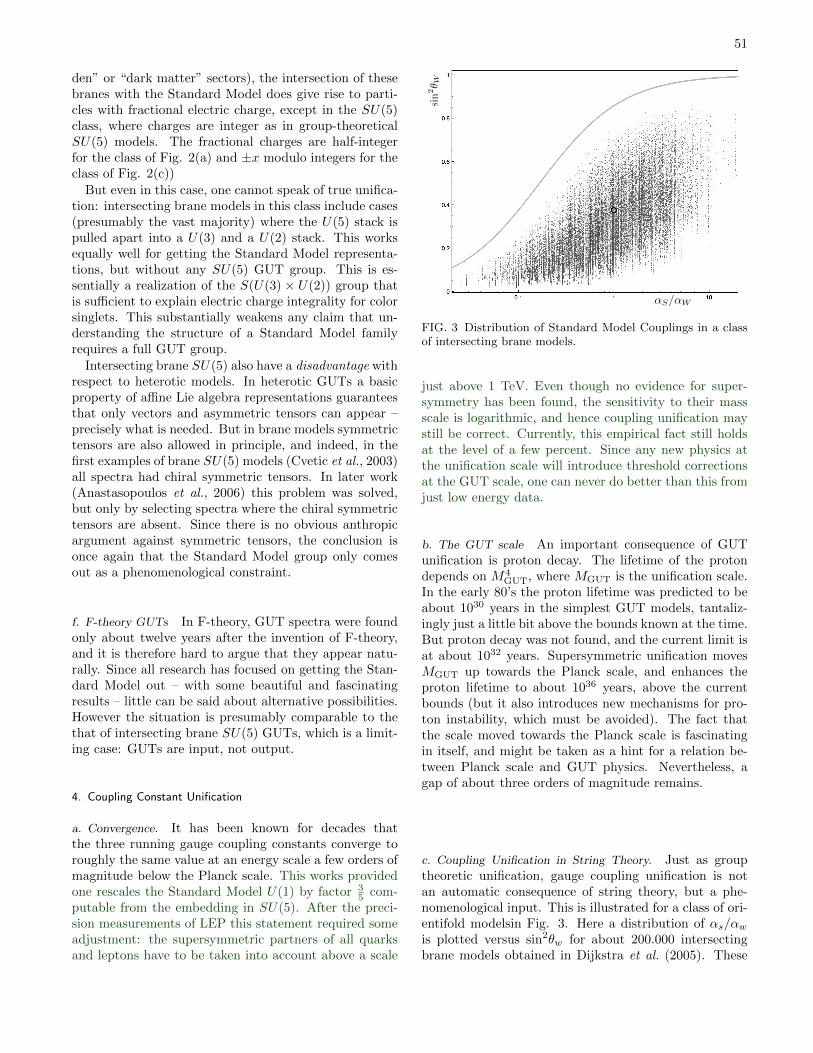
51

den” or “dark matter” sectors), the intersection of thesebranes with the Standard Model does give rise to parti-cles with fractional electric charge, except in the SU(5)class, where charges are integer as in group-theoreticalSU(5) models. The fractional charges are half-integerfor the class of Fig. 2(a) and ±x modulo integers for theclass of Fig. 2(c))

But even in this case, one cannot speak of true unifica-tion: intersecting brane models in this class include cases(presumably the vast majority) where the U(5) stack ispulled apart into a U(3) and a U(2) stack. This worksequally well for getting the Standard Model representa-tions, but without any SU(5) GUT group. This is es-sentially a realization of the S(U(3) × U(2)) group thatis sufficient to explain electric charge integrality for colorsinglets. This substantially weakens any claim that un-derstanding the structure of a Standard Model familyrequires a full GUT group.

Intersecting brane SU(5) also have a disadvantage withrespect to heterotic models. In heterotic GUTs a basicproperty of affine Lie algebra representations guaranteesthat only vectors and asymmetric tensors can appear –precisely what is needed. But in brane models symmetrictensors are also allowed in principle, and indeed, in thefirst examples of brane SU(5) models (Cvetic et al., 2003)all spectra had chiral symmetric tensors. In later work(Anastasopoulos et al., 2006) this problem was solved,but only by selecting spectra where the chiral symmetrictensors are absent. Since there is no obvious anthropicargument against symmetric tensors, the conclusion isonce again that the Standard Model group only comesout as a phenomenological constraint.

f. F-theory GUTs In F-theory, GUT spectra were foundonly about twelve years after the invention of F-theory,and it is therefore hard to argue that they appear natu-rally. Since all research has focused on getting the Stan-dard Model out – with some beautiful and fascinatingresults – little can be said about alternative possibilities.However the situation is presumably comparable to thethat of intersecting brane SU(5) GUTs, which is a limit-ing case: GUTs are input, not output.

4. Coupling Constant Unification

a. Convergence. It has been known for decades thatthe three running gauge coupling constants converge toroughly the same value at an energy scale a few orders ofmagnitude below the Planck scale. This works providedone rescales the Standard Model U(1) by factor 3

5 com-putable from the embedding in SU(5). After the preci-sion measurements of LEP this statement required someadjustment: the supersymmetric partners of all quarksand leptons have to be taken into account above a scale

S/W

sin

2 W

FIG. 3 Distribution of Standard Model Couplings in a classof intersecting brane models.

just above 1 TeV. Even though no evidence for super-symmetry has been found, the sensitivity to their massscale is logarithmic, and hence coupling unification maystill be correct. Currently, this empirical fact still holdsat the level of a few percent. Since any new physics atthe unification scale will introduce threshold correctionsat the GUT scale, one can never do better than this fromjust low energy data.

b. The GUT scale An important consequence of GUTunification is proton decay. The lifetime of the protondepends on M4

GUT, where MGUT is the unification scale.In the early 80’s the proton lifetime was predicted to beabout 1030 years in the simplest GUT models, tantaliz-ingly just a little bit above the bounds known at the time.But proton decay was not found, and the current limit isat about 1032 years. Supersymmetric unification movesMGUT up towards the Planck scale, and enhances theproton lifetime to about 1036 years, above the currentbounds (but it also introduces new mechanisms for pro-ton instability, which must be avoided). The fact thatthe scale moved towards the Planck scale is fascinatingin itself, and might be taken as a hint for a relation be-tween Planck scale and GUT physics. Nevertheless, agap of about three orders of magnitude remains.

c. Coupling Unification in String Theory. Just as grouptheoretic unification, gauge coupling unification is notan automatic consequence of string theory, but a phe-nomenological input. This is illustrated for a class of ori-entifold modelsin Fig. 3. Here a distribution of αs/αwis plotted versus sin2θw for about 200.000 intersectingbrane models obtained in Dijkstra et al. (2005). These

52

spectra are of the Madrid model type depicted in Fig.2(a). Since the gauge couplings are not related, onewould not expect them to respect gauge coupling uni-fication, and indeed they do not. One gets a broad cloudof points around the GUT point, indicated by the blackcircle. In this corner of the landscape, coupling unifica-tion is a mere coincidence.

In corners of the landscape with group-theoretic GUTunification, coupling unification is often problematic.This can perhaps be attributed to the fact that stringtheory is simply more constraining than field theory, butit is still an indication that the perfect string-GUT hasnot yet been found.

Heterotic GUTs predict a value for the unification scalethat is substantially too large. In F-theory GUTs thebreaking of the SU(5) GUT group is usually achieved nei-ther by Higgses in the (24) (as in field theory) nor by Wil-son lines (as in heterotic strings) but by U(1) flux in thehypercharge direction (see however (Marsano et al., 2013)for an F-theory example with Wilson line breaking). Thismay help solving the notorious doublet-triplet splittingproblem, but also spoils coupling unification (see Blu-menhagen (2009) and also Donagi and Wijnholt (2011a)for a discussion of various contributions to thresholds).Since there are often exotics that can contribute to therunning it may still be possible to match the observedlow energy couplings, but this turns the apparent con-vergence into a strange accident.

d. Unification versus anthropic arguments. Coupling con-stant unification could lead to a clash between anthropictuning and fundamental symmetries. If the low energyvalues of the three couplings g1, g2 and g3 are all tightlyanthropically constrained, it would be strange if theycould still meet each other at a higher scale. Put differ-ently, to optimize the Standard Model for life, it would bebetter not to be constrained by a coupling constant rela-tion, unless this is an inevitable feature of a fundamentaltheory. In the string landscape, it is not.

Of the three constants, g3 is indeed anthropically con-strained. It determines ΛQCD and the proton mass. Wewill discuss this in section V.C. The weak coupling g2

is much less constrained: thresholds of weak decays aremuch more important than the decay rates themselves.The constraints on g1, or almost equivalently on α, arediscussed below. It does not appear to be tightly con-strained, except perhaps in fine-tunings of certain nu-clear levels. Unless these are much more severe than wecurrently know, coupling unification would not get in theway of anthropic constraints. It has two free parameters,a mass scale and the value of the unified coupling at thatscale, which allow sufficient freedom to tune both ΛQCD

and α. Alternatively, one could argue that the value ofΛQCD is tuned to its anthropic value by means of tuningof α, assuming Grand Unification (Carr and Rees, 1979;

Hogan, 2000).

e. Just a Coincidence? Standard model families have anundeniable GUT structure. One might have hoped thata bit more of that structure would emerge from a fun-damental theory in a “natural” way, even taking intoaccount the fact that part of this structure has anthropicrelevance. GUTs can be found in several areas of stringtheory; see Raby (2011) for a review. But a compellingtop-down argument in favor of GUTs is missing. Bothgroup-theoretical and coupling unification are options instring theory, not predictions. Nevertheless, one couldstill speculate that Grand Unification is chosen in thestring landscape either because GUTs are statistically fa-vored – despite suggestions that symmetry is not favored(Douglas, 2012) – or that it offers anthropic advantages.For example, it might turn out to play a role in inflationor baryogenesis after all, although the originally proposedGUT-based baryogenesis mechanism does not work.

But is it just a coincidence that the three running cou-pling constants seem to converge to a single point, closeto, but just below the Planck scale? It would not bethe only one. The little-known mass formula for lep-tons pointed out by Koide (1983), me + mτ + mµ =23 (√me +

√mµ +

√mτ )2, is seen by most people as a

coincidence, because it relates pole masses at differentmass scales. But it predicts the τ mass correctly with0.01% accuracy, a whole lot better than the few percentaccuracy of GUT coupling unification. Another poten-tial coincidence, allowed by the current data within twostandard deviations, is that the self-coupling of the Higgsboson might run towards zero with vanishing β-function,exactly at the Planck mass (Bezrukov et al., 2012), abehavior predicted in the context of asymptotically safegravity (see however Hebecker et al. (2012) for an alter-native idea in string theory). Note that this coincidenceis incompatible with GUT coupling unification: the lat-ter requires low-energy supersymmetry, but the formerrequires a pure Standard Model. So at least one of thesetwo coincidences must be just that.

5. The Fine-structure Constant

The fine-structure constant enters in nearly all an-thropically relevant formulas, but it is often not verysharply constrained. Rather than tight constraints, onegets a large number of hierarchies of scales, such as sizesof nuclei, atoms, living beings, planets, solar systemsand galaxies, as well as time scales and typical ener-gies of relevant processes. See Barrow and Tipler (1986);Bousso et al. (2009b); Carr and Rees (1979); and Pressand Lightman (1983) for attempts to express these scalesin terms of fundamental parameters, usually including α.

An example of a hierarchical condition is the require-

53

ment that the Bohr radius should be substantially largerthan nuclear radii, i.e. α(me/mp) 1, presumably an-thropically required, but not a very strong restriction onα. A stronger condition follows from the upper and lowerlimits of stellar masses (Barrow and Tipler, 1986)(

α2mp

me

)3/4

Nmp .M? . 50 Nmp , (5.2)

where N is the typical number of baryons in a star, N =(MPlanck/mp)

3. Requiring that the upper limit be largerthan the lower one yields α2 . 200(me/mp), or α . 0.3.See Barnes (2012) and chapter IV of Tegmark (1998) forfascinating plots of many other limits.

The value of α is constrained from above by the compe-tition between strong and electromagnetic interactions.The electromagnetic contribution to the neutron-protonmass difference is about 0.5 MeV and proportional toα. Changing α by a factor of three destabilizes the pro-ton, but this is far from determining α. In nuclei, totalstrong interaction binding energies scale with the numberof nucleons N , electromagnetic repulsion energy scalesas αN2/R, and R scales as N1/3. Hence the maximumnumber of nucleons in a nucleus scales as α−3/2 (Hogan,2000). Increasing α by a factor of three implies drasticchanges, but also here a tight bound is hard to obtain.The precise location of nuclear levels is much more sensi-tive to α, and might give tight lower and upper bounds,for example via the Beryllium bottleneck. But to drawany conclusions one would have to recompute all poten-tially relevant nuclear levels and all types of nucleosyn-thesis. As a function of α, levels may not just move out ofconvenient locations, but also into convenient locations.

A lower bound on α can be derived from limits on theCMB fluctuations Q (Tegmark and Rees, 1998). In ouruniverse, Q ≈ 10−5. If Q is too large, galaxies would betoo dense and planetary orbits would be disrupted toofrequently; if Q is too small the galaxies could be unableto form stars or retain heavy elements after a supernovaexplosion. Clearly these are not strict limits, but takingthem at face value one finds that the anthropic upperlimit on Q is ≈ 10−4, and scales with α16/7, whereas thelower limit is Q ≈ 10−6, scaling with α−1[ln(−α)]−16/9.For smaller α the upper limit decreases and the lowerlimit increases. The window closes if α is about a factorfive smaller than 1/137.04. This assumes everything elseis kept fixed. Although the origin of the α-dependenceis a complicated matter, the fact that a lower bound isobtained is ultimately traceable to the need for electro-magnetic cooling of matter in galaxy formation, and therole of electromagnetic radiation in the functioning of thesun. Obviously, switching off electromagnetism is bad forour health.

Although the fine-structure constant is obviously rele-vant in chemistry, the lack of competition with anotherforce makes this an unlikely area for fine-tunings. In

King et al. (2010) the dependence of the chemistry of life-supporting molecules on α as well as the electron/protonmass ratio is studied. This includes the bond angle andbond length of the water molecule, and many reactionenergies. Substantial changes are found only if α is in-creased by an order of magnitude or more. Ultimatelythe special properties of water (expansion upon freezing)may be destroyed, but there is no useful limit here. Itcannot be excluded that somewhere in the chemical re-action chain leading to complex biochemical moleculesthere are bottlenecks that strongly depend on α, but wemay never know.

Lieb and Yau (1988) proved the existence of an upperbound on α based on the stability of many-body systems(i.e. many nuclei and many electrons), but the value ofthat bound is too uncertain to be of any relevance.

The competition between gravity and electromag-netism in stars is another place to look for anthropic re-lations. An interesting one concerns the surface tempera-ture of typical stars compared to the ionization tempera-ture of molecules, Tion ≈ α2me. These two temperaturesare remarkably close. Since the former temperature de-pends on the relative strength of gravity and the latterdoes not, the coincidence implies a relation between thestrength of the two interactions. Equating these temper-atures gives the fascinating relation

α6

(me

mp

)2

≈(

mp

MPlanck

). (5.3)

Numerically, both sides of this relation are 4.5 × 10−20

and 7.7 × 10−20. Although this is close, the actual tem-peratures are proportional to the fourth root of thesenumbers so that the sensitivity is less than the formulasuggests (often the square of this relation is presented,making it look even more spectacular). But does thecloseness of those two temperatures have any anthropicsignificance? Carter has conjectured that it might. Dueto the temperature coincidence, typical stars are on thedividing line between radiative and convective, and heargued that this might be linked to their ability to formplanetary systems (see Barrow and Tipler (1986) andCarr and Rees (1979) for a discussion). Perhaps a morecredible relation was suggested by Press and Lightman(1983), who argued that solar radiation would either betoo damaging or not useful for photosynthesis if thesetemperatures were very different.

In a substantial part of the anthropic literature, start-ing with Carr and Rees (1979), GUT relations are usedto link the value of α to the mass of the proton via log-arithmic running. But it in the spirit of the discussionin sec. III.A it is better not to do that. In the Stan-dard Model there is a clear decoupling between knownphysics and speculative physics (GUTs or strings), andone should therefore consider unconstrained variations ofα. Such variations are physically meaningful even if we

54

find evidence for GUTs. Since the only landscape we cantalk about, the string theory landscape, does not imposeGUT unification, there is even less reason to impose itas a constraint on valid low energy physics. In the stringlandscape, there is no justification for the statement thatratio mp/MPlanck is forced to small values by tuning α(see e.g. (Hogan, 2000).

B. Masses and Mixings

1. Anthropic Limits on Light Quark Masses

In the Standard Model quark masses are eigenvalues ofYukawa coupling matrices λ multiplied by the Higgs vevv. Therefore anthropic constraints on these masses takethe form of long elongated regions in the Standard Model(λ, v) parameter space, with rescalings in λ compensatingthose of v. All constraints come from the effect of changesin the quark masses on QCD, and do not depend on theorigin of these masses.

Several slices through this parameter space have beenconsidered in the literature. One can vary Yukawa cou-plings while keeping v fixed. This allows masses of up to200 GeV in order to avoid Landau poles in the couplings.One may also vary v while keeping the Yukawa couplingsfixed. This allows arbitrarily large quark masses, but theelectron mass also varies, so that the sign of quantitieslike md−mu−me cannot be flipped. In all cases a deci-sion has to be made what to do with ΛQCD. Some authors(e.g. Agrawal et al. (1998b)) assume a fixed coupling ata high scale (inspired by GUTs) and take into accountrenormalization group corrections to ΛQCD caused by theother parameter changes. Others vary ΛQCD so that aver-age nucleon masses remain unchanged Jaffe et al. (2009).One may also simply leave ΛQCD unchanged, and varyquark masses freely. Any choice of masses can be re-alized in the Standard Model, so one could in principleexplore the full space of possibilities for all six quarks. Ifone also allows the charged lepton and neutrino massesto cover the full range, one gets a complicated patchworkof regions with different degrees of habitability. But mostresearch in this area has focused on our own neighbor-hood, assuming two or three quarks are light. An earlydiscussion of the environmental impact of fermion masses– carefully avoiding mentioning anthropic implications –can be found in Cahn (1996).

The only admissible variations in hadronic and nuclearphysics are those that can be derived from variations inthe relevant Standard Model parameters: the QCD scaleΛQCD, and the dimensionless ratios

mu

ΛQCD,

md

ΛQCD,

ms

ΛQCD, (5.4)

although we will often just write mu,md and ms. Thestrange quark is light enough to make a sizable contribu-tion to nucleon masses by virtual processes (see Kaplan

and Klebanov (1990)) and some authors take its vari-ation into account (Jaffe et al., 2009), even allowing itto become as light as the u and d quarks. In the limitmu = md = 0, the chiral limit, the theory has an exactSU(2)L×SU(2)R symmetry, which is spontaneously bro-ken. In this limit the pion, the Goldstone boson of thebroken symmetry, is exactly massless. In the real world ithas a mass proportional to

√ΛQCD(mu +md), and the

pions are the only hadrons whose mass vanishes in thechiral limit. All other hadron masses are proportional toΛQCD.

Ideally, one would like to have a contour plot of the var-ious anthropic constraints in the parameter plane (5.4).Many older papers studying these effects discuss themin terms of strong interaction parameters that cannotbe varied independently in QCD. The superior methodfor QCD computations is lattice gauge theory, because itcan in principle fully simulate the full non-perturbativetheory. In practice, however, it is limited to relativelysimple operators, and has difficulties reaching the chi-ral limit mu,md → 0 because the quark Compton wavelength exceeds the lattice size. The next best techniquein this limit is chiral perturbation theory, which treatsthe quark masses as small perturbations of the chirallimit theory. Other techniques that are used include theMIT bag model, the Skyrme model and meson-exchangenucleon-nucleon potentials.

The quark mass dependent anthropic bounds are re-lated to the existence and stability of matter relevant forcomplex chemistry and biology, the abundances of thismatter due to big bang and stellar nucleosynthesis, stel-lar lifetimes and energy production in stars, roughly inorder of decreasing anthropocentricity. Some importantpotentially catastrophic boundary lines one may crosswhen changing parameters are:

• Instability or absence of hydrogen (1H). At this

boundary line our kind of life ceases to exist, butthere is no good reason why deuterium (or eventritium) could not take over its role in biochem-istry. Some life forms on earth tolerate heavy wa-ter quite well, and did not even evolve in a puredeuterium environment. A bigger worry is stellarburning, which in our universe relies heavily on hy-drogen fusion, and would be drastically different.Even without hydrogen there are still plenty of al-ternatives, but it is not clear whether such starswould have the right lifetimes and other propertiesto allow biochemical evolution. Finally, beyond thehydrogen stability line the neutron becomes stable,and on free neutron background can have a varietyof nasty consequences (Cahn, 1996; Hogan, 2006).Note that Hydrogen instability by electron captureoccurs before free proton instability, because thelatter costs 2mec

2 more energy.

• Instability of all di-nucleons. Beyond this line any

55

kind of synthesis of heavier elements from nucle-ons would have to start with three-body processes.In our universe stable deuterium serves as a step-ping stone. Its importance can be observed in thedeuterium bottleneck in nucleosynthesis. Althoughdeuterium is stable, it is disintegrated by photons.Therefore 4He synthesis only starts after the pho-ton density has dropped sufficiently. Even with-out stable deuterium, nucleosynthesis in stars maystill be possible in extremely dense environments.Furthermore, even an unstable, but long-lived deu-terium would still enhance the rates. But in anycase, beyond the di-nucleon stability line we are interra incognita.

• Instability or all hydrogen isotopes. Beyond thisline there is no stable hydrogen, deuterium or tri-tium (nor higher isotopes). One would have toargue that life can be based purely on complexmolecules without hydrogen of any kind.

• Instability of all heavy elements. Beyond this lineany elements beyond Helium become unstable. Itdoes not matter much which one we choose, becausetheir instability boundaries are close to each other.So one can use 12

6 C (one of the most strongly boundones) as a benchmark. The instability of these el-ements would deprive us of any scenario for theexistence of complexity. Low abundance of theseelements is a less serious issue, because it is hardto decide what the minimal required abundance is.

Now let us see how these lines are crossed if we varyStandard Model parameters. It is convenient to considervariations along the mu−md and mu +md axes (isospinviolating and isospin preserving), because the effects ofthese variations are rather different.

a. The proton-neutron mass difference. The most obviousfeature of the quark masses is the extremely small upquark mass. This is especially noteworthy since in thetwo heavy families the charge 2

3 quarks are considerablyheavier than the − 1

3 quarks. If the up and down quarkmasses were equal the proton is expected to be heavierthan the neutron because of the larger electromagneticrepulsion. The relevant parameter for weak decay of theproton or neutron is ∆ = mn −mp −me = .782, in ouruniverse. We will keep neutrino masses negligibly smallin this section. To relate ∆ to quark masses we haveto overcome the problem that quarks are confined, sothat their masses can only be measured indirectly. Fur-thermore, like all Standard Model parameters, the quarkmasses depend on the energy scale at which they aremeasured. The Particle data group gives the followingmasses for the three light quarks (in the MS scheme at a

scale of ≈ 2 GeV)

mu= 2.3+0.7−0.5MeV

md= 4.8+0.7−0.3 MeV

ms= 95± 5MeV

The scale at which these are defined is not the rightone for computing nucleon masses. For example, the pro-ton neutron mass difference has a contribution equal tomu −md, provided one uses quark masses at the correctscale. But the exact scale is hard to determine, and run-ning the quark masses to low energy scales is complicatedbecause perturbation theory breaks down. An empiricalway of dealing with this is to scale the mu−md mass dif-ference so that it equals the proton neutron mass differ-ence minus the estimated electromagnetic contribution.The latter is εEM ≈ .5 MeV, and is to first approximationproportional to αΛQCD (see (Quigg and Shrock, 2009) formore details). Hence the mass difference, in terms of thequarks masses given above, is

mn −mp = Z(md −mu)− εEM (5.5)

Here Z is an empirical scale factor, relating quark massesdefined at some high scale to the observed mass differ-ence. This parametrizes renormalization group running,which cannot be reliably calculated at low energy. Theelectromagnetic mass difference εEM ≈ 0.5 MeV is to firstapproximation proportional to αΛQCD (see Quigg andShrock (2009) for more details). For the quark massesat 2 GeV quoted by the Particle Data Group (Beringeret al., 2012) one gets Z = 0.7.

The aforementioned hydrogen stability line is crossedwhen this quantity changes sign. What happens afterthat is qualitatively clear. As we move towards morenegative values all nuclei become unstable, because theproton-neutron mass difference overcomes the bindingenergy and protons inside nuclei can decay. Analogously,if we increase mn − mp − me the neutron becomes lessstable and can decay within nuclei. Since nuclei withonly protons do not exist, this implies also that all nucleidecay.

If md −mu is increased, the neutron becomes less sta-ble, so that it starts decaying within nuclei. Since neu-trons are required for nuclear stability, this eventuallyimplies instability of all nuclei. If md −mu is decreased,the proton becomes unstable. First the hydrogen atombecomes unstable against electron capture, for a slightlyhigher value the free proton can decay, and eventuallyall nuclei become unstable. It is convenient to express alllimits in terms of the available energy, ∆ = mn−mp−me

in neutron decay. We will assume that neutrino massesremain negligible. From electron capture and β decay ofnuclei one gets respectively the following limits

M(A,Z)−M(A,Z−1) < δ(∆) < M(A,Z+1)−M(A,Z).

56

The masses M(A,Z) used here are atomic masses, andhence include electron masses. Changes in atomic bind-ing energies are ignored. Furthermore it is assumed herethat the proton or neutron are not ejected from thenucleus. This would lead to only marginally differentbounds, c.f. Jaffe et al. (2009). Near the nuclear stabil-ity line the first bound is usually negative and the secondusually positive. If one of these limits is exceeded, theatom (A,Z) is not stable.

To obtain exact quantitative results for these thresholdsone has to take into account changes in binding energiesas a function of the quark masses. This effect is probablysmall (and zero if only me is varied) because the resultdepends only on differences in binding energy of nucleiwith the same numbers of nucleons and the strong forceis isospin invariant. One may hope that the changes areminimized if mu + md is kept fixed, because then themass of the pions and several other relevant mesons doesnot change, and hence binding energies may not changemuch either. But it is not always possible to keep mu +md fixed, and vary mu − md while keeping the massespositive.

Keeping all these caveats in mind, we get the followinglimits for some nuclei of interest:

1H 0 < ∆2H − 2.2 MeV < ∆ < 2.2 MeV3H − 8.5 MeV < ∆ < .762 MeV

4He − 22.7 MeV < ∆< 23.6 MeV126C − 12.6 MeV < ∆ < 18.12 MeV

147N .62 MeV < ∆ < 5.92 MeV

168O − 9.6 MeV < ∆ < 16.2 MeV

To obtain absolute bounds one should also considerproton-rich or neutron-rich nuclides that are not stablein our universe, but may be stable for different valuesof ∆, such as 9

6C. In Agrawal et al. (1998b) argumentsare given against the stability of proton rich (Z N)nuclei. Even taking all this into account, the maximumvariation in ∆ is about ±25MeV (which translates to ±35for the quark masses given earlier). Beyond that no sta-ble nuclei exist. This is a very conservative bound. Longbefore reaching this bound catastrophic changes occur,and there is no guarantee that the few stable nuclei canactually be synthesized.

Note that only the linear combination mn −mp −me

is bounded by these arguments. (Hogan, 2000) has ob-served that the reaction

p+ p→ D + e+ + ν (5.6)

is sensitive to mn−mp+me, and shuts down if this quan-tity is increased by more than .42 MeV. This reaction isa step in hydrogen burning in the sun and hence this isdefinitely a boundary of our domain in parameter space.

However, (Weinberg, 2005) has pointed out that one re-place the outgoing e+ by an ingoing e−. The resultingthree-body interaction also does the job (although lessefficiently), but only restricts mn −mp −me.

b. Nuclear binding. While it is intuitively obvious thatincreasing or decreasing mu −md by a few tens of MeVin both directions will lead to instability of all nuclei, thisis far less obvious for variations in mu+md. An intuitiveargument is suggested by the lightness of the pion. Thepion mass increases with

√mu +md, which decrease the

range of the one-pion exchange potential, and this couldmake nuclei less stable. But one-pion exchange is not acorrect description of nuclear physics. In the literature,estimates have been given of the effect of quark masschanges on binding of heavy nuclei based on effectivefield theory and models for nuclear matter. In Damourand Donoghue (2008) the binding energy per nucleon forheavy nuclei (16O and 208Pb were used as benchmarks)was studied as a function of scalar and vector contactinteractions. These give contributions to the binding en-ergies that are large, and opposite in sign. Scalar in-teractions give a negative contribution that is an orderof magnitude larger than the actual binding energy, andreceive important contributions from two-pion exchange.The latter decreases with increasing pion mass. Becauseof the large cancellations, only a moderate increase inpion mass would make the positive contributions over-whelm the negative one and destabilize nuclei. Thesearguments may not convince QCD purists, but do theyprovide a rationale for substantial dependence of nuclearbinding on mu +md. According to these authors, a con-servative estimate for the maximum allowed increase inmu +md is about 64%.

c. Bounds on the Higgs vev. The limits discussed aboveare often expressed in terms of allowed variations of theHiggs vacuum expectation value, under the assumptionthat the Yukawa couplings are kept fixed. The upperbound of ∆ of 25 MeV translates into an upper boundon v/v0 (where v0 is the observed value) of about 20. Thenegative lower bound has no effect, because v cannot benegative. But if one just requires stability of hydrogen1H under electron capture, the bound is ∆ > 0, whichimplies (but note that the error in md −mu is huge)

v

v0>

εEM

Z(md −mu)−me≈ 0.4 . (5.7)

Here we used the method of Damour and Donoghue(2008); in Hogan (2006) the lower bound was estimatedas 0.6 ± 0.2 using lattice results on isospin violation(Beane et al., 2007). If we also use the more model-dependent nuclear binding bounds, the window for v/v0

is quite small, 0.4 < v/v0 < 1.64.

57

Limits on v/v0 were first presented by Agrawal et al.(1998b), who estimated an upper limit v/v0 < 5, from acombination of the two arguments on stability of nucleidiscussed above. In this work the Higgs mass parame-ter µ2 is varied over its entire range, from −M2

Planck to+M2

Planck, while keeping all other parameters in the La-

grangian fixed. Then if µ2 is negative, v =√−µ2/λ,

and v/v0 can lie anywhere between 0 and 1017 GeV. Theanthropic range is in any case extremely small in com-parison to the full allowed range.

Because of the possible implications for the gauge hi-erarchy problem, it is important to exclude the entirerange, not just the small region around us. If v is in-creased to much larger values, there is still an importantqualitative change. As the md −mu mass differences in-creases, at some point the lightest three up-quark statewill be lighter than the proton. This is the ∆++, about300 MeV heaver than the proton because of QCD effects.There is a small range where both the proton and the∆++ are stable. If there are no nuclear bound states (asseems plausible) of these objects this universe is compa-rable to a pure helium or helium plus hydrogen universe,and probably lifeless (Agrawal et al., 1998b).

One may apply analogous arguments in the two-Higgscase. In many models, there are separate Higgs bosonsfor up and down quarks. Then an interesting variationis to keep all Yukawa couplings fixed and allow the twoHiggs scales to vary independently. Then larger hierarchyin the up-quark sector is taken as a given. (Barr andKhan, 2007) argue that rough equality of mu and md isanthropically required, so that the large ratio of the topquark and bottom quark mass are predicted.].

Although the weak scale is linked to the Higgs mech-anism, which operates for µ2 < 0, it is also interestingto see if the mechanism itself is anthropically needed,in other words if life plausibly exists for µ2 > 0. Forpositive µ2 the Higgs potential does not have the famil-iar “Mexican hat” shape, but now the weak interactionsymmetry is broken by quark condensates, 〈qq〉 ∝ f3

π ,where fπ is the pion decay constant. (see Quigg andShrock (2009) for a interesting discussion of closely re-lated cases.) This is the usual chiral symmetry breakingmechanism of QCD, except that all quark flavors partic-ipate democratically, because they are all massless priorto chiral symmetry breaking. These vacuum expectationvalues feed into the Higgs system via the Yukawa cou-plings, and the dominant contribution comes from thetop quark. This generates a vev for the Standard ModelHiggs boson, which in its turn generates all quark andlepton masses via the Yukawa couplings. The Higgs vac-uum expectation value is given by v = λt(f

3π/µ

2) forµ2 >> f2

π (for simplicity we will focus on this case here).The pion decay constant is proportional to ΛQCD, which,in keeping with the philosophy behind this work, is keptfixed. Hence all quark and lepton masses are computablenumbers, and they are smaller by a factor ≈ 10−9 than

the values observed in our universe. In particular theelectron mass is reduced by a factor 109, and hence thecharacteristic time scale of chemistry becomes larger bythe same factor, while biochemical energies and tempera-tures are reduced. Agrawal et al. (1998b) argued that inthat case it would take too long for the universe to cooloff sufficiently to allow biochemical life; stars would haveburned out already. They also point out that most pro-tons would have decayed, but this can be circumventedeasily by not having Grand Unification.

An important loophole in this argument was pointedout by Barr and Khan (2007). The original discussionignored accelerated expansion, which had not been dis-covered yet. In a universe with accelerated expansioncooling occurs much more rapidly, which invalidates theargument. However Barr and Khan (2007) point anotherlimit: if the electrons mass decreases by a factor y plan-ets increase in size by a factor y3, and their average den-sity can drop below the cosmological constant density.In that case the expansion would presumably rip themapart. Note that the density of matter in Planck units is≈ (αme)

3mp = 2.2× 10−93.

d. Big Bang Nucleosynthesis. Understanding the synthe-sis of heavy elements in our universe has been one ofthe great successes of last century physics. It is a com-plicated and delicate process, starting with production ofsome light elements during the hot phase of the Big Bang,followed by synthesis of heavier elements in stars and su-pernovae. Several of these processes are rather sensitiveto the values of Standard Model parameters, such as thelight quark masses, ΛQCD, α, and the scale and strengthof the weak interactions. It is important to distinguishobservational and anthropic constraints.

In our kind of universe Big Bang Nucleosynthesis(BBN) leads mainly to production of 4He, 1H, and smallamounts of deuterium, tritium and lithium. The mainpotential impact of BBN is therefore a destructive one:there might be too little hydrogen left. A hydrogen-lessuniverse is anthropically challenged, but there are no ob-vious arguments against the other extreme, a helium-lessuniverse (Carr and Rees, 1979). Helium is needed as astepping stone to heavier elements, but can also be madein stars.

In which extreme we end up is to a large extent de-termined by the electroweak freeze-out temperature (thetemperature where the rate of electroweak n↔ p conver-sions drops below the expansion rate)

Tf ≈(GNG4F

) 16

= (v/MPlanck)13 v ≈ 0.66 MeV , (5.8)

where v is the Higgs vev. At temperatures above Tf

protons and neutrons are in thermodynamic equilib-rium, and their ratio is given by a Boltzmann factor,

58

n/p = exp[−(mn − mp)/Tf ]. At Tf the ratio n/p is“frozen”, and only decreases slightly because of neutrondecay. After freeze-out, the outcome of BBN is deter-mined only by strong interactions, which conserve flavor.They burn essentially all remaining baryons into helium,removing equal amounts of p and n. Hence one ends upwith a fraction of hydrogen equal to (p − n)/(p + n) atfreeze-out. This fraction approaches the danger zone (no1H) if (

mn −mp

v

)(MPlanck

v

) 13

→ 0. (5.9)

This remarkable quantity involves all four interactions,since mn − mp receives contributions from quark massdifferences (proportional to v) and electromagnetic ef-fects. The latter are proportional to ΛQCD, and in thisway BBN is sensitive to changes in that scale (Knellerand McLaughlin, 2003).

There are two remarkable order of magnitude coinci-dences here: Tf ≈ mn−mp, and the neutron lifetime τn isof order the duration of nucleosynthesis. It is not clear ifthese have any anthropic relevance. Increasing mn −mp

and decreasing τn to more “natural” values leads to alarger fraction of 1H. It is almost as if these quantitiesare anti-anthropically tuned! The hydrogen fraction isonly moderately sensitive to increases of v, since for largev the dependence cancels out in the first factor, and theneutron lifetime decreases. Even if we ignore the latter,an increase of v by a factor 1000 decreases the mass frac-tion of hydrogen from 75% to 6%. It is hard to arguethat this would not be enough. It is fascinating that Tf

and mn − mp have the same order of magnitude, eventhough they have a completely different origin. However,the anthropic impact of this coincidence is not so clear,as long as no thresholds are crossed (especially nucleonand di-nucleon stability, see below). Note that to get intothe danger zone one would have to make mn −mp evensmaller than it already is: this would be anti-anthropictuning! The other natural way to get into the dangerzone is to enlarge v. But for large v the dependence on vcancels out in the first factor. Consequently an increaseof v by a factor 103 still gives a universe with about 2%of hydrogen, and it is hard to argue convincingly thatthis is not enough. Another interesting fact is that inour universe the free neutron decays with a life-time ofabout 880 seconds, remarkably close to the duration ofBig Bang Nucleosynthesis, given the wide range of weakinteraction lifetimes. If the neutron decayed much faster,we would end up with a universe consisting mostly outof hydrogen.

No strict limit will follow from such an argument, but itis quite possible that the number of observers per baryondrops off sharply in the limit of vanishing hydrogen abun-dance. In our universe we have ended up with about 75%hydrogen and 25% Helium. It is possible that the opti-mum is somewhere near this point.

e. Few-Nucleon systems. The stability properties of twoand three nucleon systems certainly look fine-tuned in ouruniverse: Deuterium is just bound by 1.1 MeV per nu-cleon, di-protons and di-neutrons are just not bound byabout 60-70 keV. Tritium is much more strongly boundthan deuterium but β-decays to 3He. But a decrease ofthe neutron-proton mass difference by a mere 20 keV(!)would make it stable. Once β-decay is forbidden, tritiummay be stable even after the deuterium stability line hasbeen crossed, because of its higher binding energy.

Possible consequences of tritium stability on stars,apart from its potential role in chemistry, were discussedby Gould (2012). This author speculates that changesin fusion processes in stars could affect the formation ofplanets.

In much of the literature on anthropic tuning one findsthe claim that stability of the di-proton would have ahuge effect on BBN. The idea was that all protons wouldbe fused to di-protons (which then decays to Deuterium,which is then burned into Helium), so that no 1H Hy-drogen would be left (a stable di-neutron may also haveobservable effects (Kneller and McLaughlin, 2004), butthey are less likely to have anthropic implications.)

This claim is based on the mistaken assumption thatthe di-proton production cross-section should be compa-rable to that of deuterium. However, there are impor-tant differences: Coulomb repulsion for pp and identicalparticle effects (Bradford, 2009; MacDonald and Mul-lan, 2009). In particular, deuterium and di-proton/di-neutron have different spin wave functions, because theS = 1 state of the deuteron (the lowest state for dy-namical reasons) is forbidden for two identical nucleons.Although these authors consider illegitimate variations

of the “old-fashioned effective strong coupling constant”(not αs) or nuclear potentials, the main point appearsto be a valid one: even if di-nuclei are stable, this willnot strongly affect big bang nucleosynthesis. But thesearguments do not demonstrate that there are any validparameter values for which the di-nucleons are stable.

Stability of di-nuclei does have a huge impact on stars.If the di-proton were stable, the deuteron production ratecould be ten orders of magnitude larger than in our uni-verse, with unknown consequences (Bradford, 2009). Sothe di-proton stability line – if it exists at all – marks theend of our region and the beginning of terra incognita.

The tritium stability line can undoubtedly be crossedby changing the quark masses, but for the other stabilitylines this cannot be decided without a more detailed lookat nuclear binding. The dependence of binding on quarkmasses is still uncertain. For instance, it is not clearif the deuteron is bound in the chiral limit; see Beaneand Savage (2003a,b); and Epelbaum et al. (2003). Forrecent results and references on the impact of variationsof quark masses on nuclear forces and BBN see Berengut

59

et al. (2013)5.

There are many studies of the effect of quark masseson nuclear binding in order to constrain possible varia-tions of parameters since the time of BBN and/or solvethe primordial Lithium problem. According to Flam-baum and Wiringa (2007) an upward change of the pionmass of 60% would make the deuteron unbound, whereasa downward change by 15% would make the di-neutronbound; see also Carrillo-Serrano et al. (2012)

Lattice computations are still in their infancy, and can-not get close enough to small quark masses (Beane et al.,2012; Chen et al., 2012a; Ishii et al., 2007; Yamazakiet al., 2011). A result that might have implications in thiscontext was presented in (Braaten and Hammer, 2003),who pointed out that QCD is remarkable close to a criti-cal infrared limit cycle in the three nucleon system, whichcan possibly be reached by small quark mass variations.

Properties of few-nucleon systems are potentially an-thropically relevant, and appear to be fine-tuned, but toolittle is known about either to draw firm conclusions.

f. The triple alpha process. BBN ends with a universeconsisting mainly of protons, electrons and α-particles.Fusion to heavier elements is inhibited because there areno stable nuclei with A = 5 or A = 8. Hence there are nopaths with only two-particle reactions leading to heaviernuclei. The most obvious path to 12C is α + α → 8Be,followed by 8Be + α → 12C. But 8Be is unstable witha lifetime of about 10−16 seconds, so this does not lookpromising.

There are at least three remarkable facts that improvethe situation. First of all, the 8Be ground state is a verynarrow resonance in the αα-channel, enhancing the firstprocess. The narrowness of this resonance is due to aremarkable tuning of strong versus electromagnetic in-teractions (Higa et al., 2008). Secondly, there is a reso-nance of 12C (the second excitation level) that enhancesthe second process. Finally, a logical third step in thischain, 12C + α → 16O, is not enhanced by a resonance.If that were the case all 12C would be burned to 16O.Indeed, there is a resonance in 16O (at 7.10 MeV) thatlies close to, but just below the 12C +α threshold at 7.16MeV.

5 Many papers studying the impact of variations on BBN or thetriple-alpha process consider observational constraints, for thepurpose of detecting variations in constants of nature. Thisshould not be confused with anthropic constraints. Anothersource of confusion is that some authors convert variations inthe strong force to variations in α via an assumed GUT relation,as explained in Calmet and Fritzsch (2002) and Langacker et al.(2002). This greatly enhances the sensitivity to variations in α,see e.g. Ekstrom et al. (2010).

The reaction rate of the triple-α process is proportionalto (Burbidge et al., 1957)

r3α ∝ Γγ

(NαkBT

)3

e−ε/kBT , (5.10)

where ε ≈ 397 keV is the energy of the 12C resonanceabove the 3α threshold, Γγ is de width of its radiativedecay into 12C and Nα is the α-particle number den-sity. Since the participating α-particles are from the tailof a thermal distribution, raising the resonance energydecreases the 12C production rate rapidly, lowering it in-creases 12C production. This formula enters into the cal-culation of element abundances, which can be comparedwith observations. Assuming 12C synthesis takes placein the late stage of red giants at temperatures of order108K one can then fit ε to the observed abundances, bymoving the resonance along the exponential tail. Thiswas done by Hoyle (1954) and led to a prediction for ε,which in its turn led to a prediction of an excited level of12C at 7.65 MeV above the ground state. This resonance(now known as the “Hoyle state”) was indeed found. Foran excellent account of the physics and the history seeKragh (2010).

Since the abundance of Carbon is at stake, it is tempt-ing to draw anthropic conclusions. But Hoyle’s resultis merely an observational statement, not an anthropicstatement. Determining the true anthropic relevance ofthe Hoyle state is a difficult matter. Changing the res-onance changes the stars themselves, because the triple-alpha process is their source of energy. One must takeinto account not only 12C production, but also the burn-ing of 12C to 16O. These processes are all strongly tem-perature dependent, and may occur in a variety of typesof stars of very different masses. Even if most 12C weobserve is made in red giants, one must allow for the pos-sibility that in different universes other processes domi-nate. Furthermore, an energy level of 12C is not a freeparameter; one would really have to study the full, com-bined effect of changing Standard Model parameters onall relevant processes. One has to make assumptionsabout the chances for life in an environment with dif-ferent 12C to 16O ratios. Even if all 12C is burned to 16Oand heavier elements, one has to rule out the possibilityof Carbon-less life based on heavier elements. It is there-fore not surprising that different authors have come torather different conclusions.

Without the Hoyle state the third excited state of 12Cat 9.64 could take over its role, but then stars wouldburn at such high temperatures that even primordial 12Cwould be destroyed (Livio et al., 1989). Hence the exis-tence of the Hoyle state is indeed important for our kindof life. However, according to Weinberg (2005) the exis-tence of the Hoyle state in 12C can be understood on thebasis of collective dynamics of α-particles. The same αα-potential that produces the 8Be ground state would give

60

rise to nα oscillator-like excitations in A = 4n,Z = 2nnuclei, appearing above the nα threshold. This demysti-fies the existence of the Hoyle state for n = 3, but doesnot predict its location relative to (A − 4, Z − 2) + αthreshold. Both the sign and the size of that differenceare crucial.

The quantitative effect of changes of the resonance en-ergy away from its value of 288 keV was studied by Livioet al. (1989). These authors varied the excitation level inlarge steps, and found that for an upward change of 277keV or more very little 12C is produced, but for an in-crease of 60 KeV they did not find a significant change. Adownward variation by 60 keV led to a four-fold increasein the 12C mass fraction, suggesting that we are not liv-ing at the anthropic optimum (“things could be worse,but they could easily be much better”, in the words ofthe authors); but this statement does not take into ac-count the reduction of Oxygen. Schlattl et al. (2004),using more advanced stellar evolution codes that followthe entire evolution of massive stars, found that in a bandof ±100 keV around the resonance energy the changes inabundances are small.

Compared to ε = 397 keV this suggest a tuning of nomore than about 20%, but the really relevant question ishow 12C and 16O production vary as function of StandardModel parameters. This is an extremely complicated is-sue, since a proper treatment requires keeping track of allchanges in nuclear levels, the rates of all processes andthe effect on models for stellar evolution. Processes thatare irrelevant in our universe may become dominant inothers. Most work in this area has focused just on findingout how the Hoyle state moves.

To decide how fine-tuned this is one would like to seethe effect of Standard Model parameter changes. A firststep in that direction was made by Oberhummer et al.(2000), who studied the effect on the resonance energyof rescalings of the nucleon-nucleon and Coulomb poten-tials. They concluded that changes of 0.5% and 4% re-spectively led to changes in C or O abundances by sev-eral orders of magnitude (factors 30 to a 1000). Thesechanges correspond to shift in the Hoyle state energyof about 130 keV (Schlattl et al., 2004), and hence thisconclusion is in rough agreement with Livio et al. (1989).However, in Schlattl et al. (2004) the same group consid-ered a more sophisticated model of stellar evolution (in-cluding the possibility of C-production in helium flashes),and concluded that their conclusions on fine-tuning were“considerably weakened”.

Although rescaling of the nuclear force is more mean-ingful then an ad hoc rescaling of a nuclear energy level, itis still not a valid parameter change. A step towards thatgoal was made by Epelbaum et al. (2013). These authorsinvestigate the quark mass dependence of the 12C and16O productions rates using “nuclear lattice simulations.”This is a combination of chiral effective field theory withsimulations of non-perturbative nucleon-pion theory on

a lattice (not to be confused with lattice QCD). Theseauthors conclude that 12C and 16O production would sur-vive a 2% change in the light quark masses or the finestructure constant. Beyond this band (which correspondsto a change of around 100 keV in the Hoyle state energy)substantial changes can be expected.

One can try to convert these survivability bands interms of variations of the Higgs vev, the common scale ofthe quark masses. The naive expectation is that enlarg-ing the Higgs vev increases the pion mass, which weakensthe nuclear potential, which, according to Oberhummeret al. (2000), increases the resonance energy and hencelowers the C/O ratio. If one focuses only on 12C (assum-ing Oxygen can be made elsewhere), this would put anupper limit on the Higgs vev v.

Indeed, Hogan (2006) concludes that there is an upperlimit for v. Using the aforementioned simple potentialmodel for collective oscillations of α-particles suggestedby Weinberg (2005), the author estimates that the en-ergy gap between the Hoyle state and the 3α thresh-old scales with (v/v0)

12 . But since the triple alpha pro-

cess is main energy source of the star, it must scale itstemperature by the same factor to maintain equilibrium.Then the triple alpha rate, and hence the 12C produc-tion rate stays the same, but the change in temperatureaffects all other reaction rates. For reaction rates thatare not thought to be very sensitive to changes in v, likeα + 12C → 16O this implies a change in reaction ratesby a factor exp[(E/T )((v/v0)

12 − 1)], where E/T is es-

timated to be about 30. For an increase of v/v0 by 5%the 16O burning rate doubles, and most 12C is expectedto burn to 16O. For a decrease of v/v0

16O productiondecreases, but perhaps 16O could still be produced inhotter stars. Therefore Hogan (2006) only puts an upperlimit on the allowed increase of v of about 5%. This isstill an order of magnitude tighter than the upper boundon v from nuclear binding (see sect. (V.B.1.c), but thereis a disturbing discrepancy in all these estimates. Sen-sitivities differ by an order of magnitude, and there isnot even agreement on the existence of upper and lowerbounds. But Jeltema and Sher (2000), using the resultsof Oberhummer et al. (2000) mentioned above, find alower limit on v about 1% below its observed value. Notethat this lower bound is derived assuming the same physi-cal requirement, namely sufficient Carbon production. Inother words, Jeltema and Sher (2000) and Hogan (2006)find a different sign for the dependence of the Carbonproduction rate on v.Although the discrepancy may bedue to the different treatment of nuclear forces, there isanother difference: in the first work the strong interac-tion scale is kept fixed, whereas in the second the strongcoupling is kept fixed at the GUT scale. Then ΛQCD

changes due to changes in quark mass thresholds affect-ing the running of αs. This appears to be the dominanteffect.

Expressed in terms of changes if v, the results of Epel-

61

baum et al. (2013) indicate that the Hoyle state energygoes up when v is increased, but there are contributingterms with different signs and large errors. Therefore theopposite dependence is not entirely ruled out.

The Hoyle resonance has also received attention be-cause it may give bounds on temporal variations of con-stants of nature. If some constants were different duringthe early stages of the universe this would affect 12C or16O production, and this may lead to disagreement withobserved abundances. To investigate this (Ekstrom et al.,2010) have studied massive (15 and 60 M) populationIII stars believed to be the earliest ones formed in our uni-verse. To parametrize variations they allow a rescaling ofboth the strong and the Coulomb interaction potential.They find a sensitivity at the per mille level to changesin the strong force. Note however that these are observa-tional bounds and not anthropic bounds, and hence it isnot surprising that they are tighter than those mentionedabove. These authors also give bounds on allowed frac-tional variations of the fine structure constant of order10−5, but these are obtained from the strong interactionbounds using the assumption of Grand Unification. Thedirect bounds on α are far weaker than those of strongforce variations.

In (Higa et al., 2008) the αα resonance is examinedusing effective field theory, and these authors observethe scattering length is enhanced by a factor a 1000 incomparison to its natural value. This is due to fine-tuned cancellations between several strong interactioncontributions, as well as cancellations between strong andCoulomb contributions. Since the cross section is propor-tional to the square of the scattering length, this is a hugeeffect. They also observed that an increase of the stronginteraction range by 20% would make 8Be ground statestable. This would remove the Beryllium bottleneck al-together, and lead to such drastic changes that the conse-quences are hard to estimate. Perhaps 12C could alreadybe produced in Big Bang Nucleosynthesis. If stability of8Be can be achieved within the Standard Model parame-ter space, this would turn the anthropic question up-sidedown: why do we live in a universe with 12C produc-tion bottleneck, given the absence of that bottleneck inothers?

Even the most conservative interpretation of all thiswork still implies that a minute change of v with respectto ΛQCD in either direction has drastic consequences.Note that the full scale of v/v0 goes up to 1017, andthe variations discussed above are by just a few percent.

2. The Top Quark Mass

The top quark may not seem an obvious target foranthropic arguments, but it may well be important be-cause of it large coupling to the Higgs boson, which playsa dominant role in the renormalization group running

of parameters. In supersymmetric theories, this largecoupling may drive the Higgs µ2 parameter to negativevalues, triggering electroweak symmetry breaking (seeIbanez and Ross (1982); since this work preceded the topquark discovery, the authors could only speculate aboutits mass).

The large top quark mass may also play an importantrole in the Standard Model, although the mechanism isless clear-cut, see Feldstein et al. (2006). These authorsargue that in a landscape the top quark mass is pushed tolarge values to enhance vacuum stability. This issue wasre-analyzed recently by Giudice et al. (2012) using therecent data on the Higgs mass and under somewhat dif-ferent assumptions. They conclude that the quark massesmay be understood in terms of a broad distribution cen-tered around one GeV, with the light quark masses andthe top quark mass as outliers, pushed to the limits byanthropic (atomic or stability) pressures.

3. Charged Lepton Masses

The electron mass is bounded from above by the limitsfrom nuclear stability already discussed in section V.B.If the electron is a factor 2.5 heavier, hydrogen 1H is un-stable against electron capture; if one can live with tri-tium the bound goes up to about 10 MeV. Beyond thatbound most heavy nuclei are unstable as well. See Jenk-ins (2009) for other, less restrictive bounds, for examplethe fact that a much heavier electron (by a factor & 100)would give rise to electron-catalyzed fusion in matter.

There are several arguments for smallness of the elec-tron mass in comparison to the proton mass. The bound(me/mp)

1/4 1 is important for having matter with lo-calized nuclei (Barrow and Tipler, 1986), but there is noclear limit. Limits on hierarchies of scales (e.g. Bohrradius versus nuclear radius, see section V.A.5) are notvery tight because the electron mass is multiplied withpowers of α.

There are also lower bounds on the electron mass, butmostly qualitative ones. Lowering the electron mass en-hances the Thomson scattering cross section that deter-mines the opacity of stars. It affects the temperature ofrecombination and all chemical and biological tempera-tures. The stellar mass window (5.2) gives a bound on me

because the lower limit must be smaller than the upperone: me > 0.005 α2mp ≈ 250 eV.

If muon radiation plays an important role in DNA mu-tations, then the location of the muon mass just belowthe pion mass would be important (see footnote 17 inBanks et al. (2004)). But the danger of anthropocentrismis enormous here.

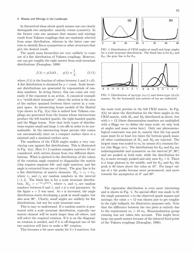
62

4. Masses and Mixings in the Landscape

In theoretical ideas about quark masses one can clearlydistinguish two antipodes: anarchy versus symmetry. Inthe former case one assumes that masses and mixingsresult from Yukawa couplings that are randomly selectedfrom some distribution, whereas in the latter case onetries to identify flavor symmetries or other structures thatgive the desired result.

The quark mass hierarchies are very unlikely to comeout of a flat distribution of Yukawa couplings. However,one can get roughly the right answer from scale-invariantdistributions (Donoghue, 1998)

f(λ) = ρ(λ)dλ , ρ(λ) ∝ 1

λ, (5.11)

where f(λ) is the fraction of values between λ and λ+dλ.A flat distribution is obtained for ρ = const. Scale invari-ant distributions are generated by exponentials of ran-dom numbers. In string theory, this can come out veryeasily if the exponent is an action. A canonical exampleis a “world-sheet instanton”, where the action is the areaof the surface spanned between three curves in a com-pact space. In intersecting brane models of the Madridtype shown in Fig. 2(a) this is indeed how Yukawa cou-plings are generated from the branes whose intersectionsproduce the left-handed quarks, the right-handed quarksand the Higgs boson. Note that both types of distribu-tions require small and large λ cut-offs in order to be nor-malizable. In the intersecting brane picture this comesout automatically since on a compact surface there is aminimal and a maximal surface area.

The smallness of the CKM angles makes a very con-vincing case against flat distributions. This is illustratedin Fig. 4(a). Here 2×2 random complex matrices M areconsidered, with entries chosen from two different distri-butions. What is plotted is the distribution of the valuesof the rotation angle required to diagonalize the matrix(this requires separate left- and right matrices, and theangle is extracted from one of them). The gray line is fora flat distribution of matrix elements, Mij = r1 + ir2,where r1 and r2 are random numbers in the interval[−1, 1]. The black line is for a scale invariant distribu-tion, Mij = e−sr1e2πir2 , where r1 and r2 are randomnumbers between 0 and 1, and s is a real parameter. Inthe figure s = 5 was used. As s is increased, the angledistribution starts developing a peak at small angles, butalso near 90. Clearly, small angles are unlikely for flatdistributions, but not for scale invariant ones.

This is easy to understand. If a random matrix is gen-erated with a scale invariant distribution, typically onematrix element will be much larger than all others, andwill select the required rotation. If it is on the diagonal,no rotation is needed, and if it is off-diagonal one of thetwo matrices will have to make a 90 rotation.

This becomes a bit more murky for 3×3 matrices, but

0 30 60 900 30 60 90

(a) (b)

FIG. 4 Distribution of CKM angles at small and large anglesfor a scale invariant distribution. The black line is for θ12 andθ23, the gray line is for θ13.

-6 -5 -4 -3 -2 -1 0 1-6 -5 -4 -3 -2 -1 0 1

FIG. 5 Distribution of up-type (u,c,t) and down-type (d,s,b)masses. On the horizontal axis powers of ten are indicated.

the main trait persists in the full CKM matrix. In Fig.4(b) we show the distribution for the three angles in theCKM matrix, with Mu and Md distributed as above, butwith s = 12 (these dimensionless numbers are multipliedwith a Higgs vev to define the mass scale; we only lookat angles and mass ratios here). Only one phenomeno-logical constraint was put in, namely that the top quarkmass must be at least ten times the bottom quark mass;all other combinations of Mu and Md are rejected. Thelargest mass was scaled to mt by means of a common fac-tor (the Higgs vev). The distributions for θ12 and θ23 areindistinguishable and symmetric on the interval [0, 90]and are peaked at both ends, while the distribution forθ13 is more strongly peaked and only near θ13 = 0. Thereis a large plateau in the middle, and for θ12 and θ23 thepeak is 40 times above the value at 45. For larger val-ues of s the peaks become more pronounced, and movetowards the asymptotes at 0 and 90.

The eigenvalue distribution is even more interestingand is shown in Fig. 5. No special effort was made to fitthe single parameter s to the observed quark masses andmixings; the value s = 12 was chosen just to get roughlyin the right ballpark, for illustrative purposes only. Notethat the difference between the two plots is entirely dueto the requirement mt > 10 mb. Renormalization grouprunning was not taken into account. This might favorlarge top quark masses because of the infrared fixed pointof the Yukawa couplings (Donoghue, 1998).

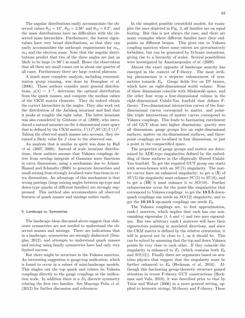
63

The angular distributions easily accommodate the ob-served values θ12 = 13, θ23 = 2.38 and θ13 = 0.2, andthe mass distributions have no difficulties with the ob-served mass hierarchies. Furthermore, the lowest eigen-values have very broad distributions, so that they caneasily accommodate the anthropic requirements for mu,md and the electron mass. Note that the angular distri-butions predict that two of the three angles are just aslikely to be large (≈ 90) as small. Hence the observationthat all three are small comes out in about one quarter ofall cases. Furthermore there are large central plateaus.

A much more complete analysis, including renormal-ization group running, was done by Donoghue et al.(2006). These authors consider more general distribu-tions, ρ(λ) = λ−δ, determine the optimal distributionfrom the quark masses, and compute the median valuesof the CKM matrix elements. They do indeed obtainthe correct hierarchies in the angles. They also work outthe distribution of the Jarlskog invariant and find thatit peaks at roughly the right value. The latter invariantwas also considered by Gibbons et al. (2009), who intro-duced a natural measure on the 4-dimensional coset spacethat is defined by the CKM matrix, U(1)2\SU(3)/U(1)2.Taking the observed quark masses into account, they ob-tained a likely value for J close to the observed one.

An analysis that is similar in spirit was done by Hallet al. (2007, 2008). Instead of scale invariant distribu-tions, these authors assume that Yukawa couplings de-rive from overlap integrals of Gaussian wave functionsin extra dimensions, using a mechanism due to Arkani-Hamed and Schmaltz (2000) to generate hierarchies andsmall mixing from strongly localized wave functions in ex-tra dimensions. An advantage of this mechanism is thatwrong pairings (large mixing angles between up-type anddown-type quarks of different families) are strongly sup-pressed. This method also accommodates all observedfeatures of quark masses and mixings rather easily.

5. Landscape vs. Symmetries

The landscape ideas discussed above suggest that elab-orate symmetries are not needed to understand the ob-served masses and mixings. There are indications thatin a landscape, symmetries are strongly disfavored (Dou-glas, 2012), and attempts to understand quark massesand mixing using family symmetries have had only verylimited success.

But there might be structure in the Yukawa matrices.An interesting suggestion is gauge-top unification, whichis found to occur in a subset of mini-landscape models.This singles out the top quark and relates its Yukawacouplings directly to the gauge couplings at the unifica-tion scale. In addition there is a D4 discrete symmetryrelating the first two families. See Mayorga Pena et al.(2012) for further discussion and references.

In the simplest possible orientifold models, for exam-ples the ones depicted in Fig. 2, all families are on equalfooting. But this is not always the case, and there aremany examples where different families have their end-points on different branes. This gives rise to Yukawacoupling matrices where some entries are perturbativelyforbidden, but can be generated by D-brane instantons,giving rise to a hierarchy of scales. Several possibilitieswere investigated by Anastasopoulos et al. (2009).

Almost the exact opposite of landscape anarchy hasemerged in the context of F-theory. The most strik-ing phenomenon is a stepwise enhancement of sym-metries towards E8. Gauge fields live on D7 branes,which have an eight-dimensional world volume. Fourof these dimensions coincide with Minkowski space, andthe other four wrap a four-dimensional volume in theeight-dimensional Calabi-Yau fourfold that defines F-theory. Two-dimensional intersection curves of the four-dimensional curves correspond to matter, and point-like triple intersections of matter curves correspond toYukawa couplings. This leads to fascinating enrichmentof old GUT ideas into higher dimensions: gravity seesall dimensions, gauge groups live on eight-dimensionalsurfaces, matter on six-dimensional surfaces, and three-point couplings are localized in four dimensions, or justa point in the compactified space.

The properties of gauge groups and matter are deter-mined by ADE-type singularities defined by the embed-ding of these surfaces in the elliptically fibered Calabi-Yau fourfold. To get the required GUT group one startswith seven-branes with an SU(5) singularity. The mat-ter curves have an enhanced singularity; to get a (5) ofSU(5) the singularity must enhance SU(5) to SU(6), andto get a (10) it must enhance it to SO(10). Furtherenhancements occur for the point-like singularities thatcorrespond to Yukawa couplings: to get the 10.5.5 down-quark couplings one needs an SO(12) singularity, and toget the 10.10.5 up-quark couplings one needs E6.

The Yukawa couplings are, to first approximation,rank-1 matrices, which implies that each has one non-vanishing eigenvalue (t, b and τ) and two zero eigenval-ues. But two arbitrary rank-1 matrices will have theireigenvectors pointing in unrelated directions, and sincethe CKM matrix is defined by the relative orientation, itwill in general not be close to 1, as it should be. Thiscan be solved by assuming that the top and down Yukawapoints lie very close to each other. If they coincide thesingularity is enhanced to E7 (which contains both E6

and SO(12)). Finally there are arguments based on neu-trino physics that suggest that the singularity must befurther enhanced to E8 (Heckman et al., 2010). Al-though this fascinating group-theoretic structure gainedattention in recent F-theory GUT constructions (Heck-man and Vafa, 2010), it was described prior to that byTatar and Watari (2006) in a more general setting, ap-plied to heterotic strings, M-theory and F-theory. These

64

authors derived the E7 structure requiring the absenceof baryon number violation dimension-4 operators.

To get non-zero values for the other masses, a mech-anism like the one of Froggatt and Nielsen (1979) wasproposed. This works by postulating one or more addi-tional U(1)’s and assigning different charges to the dif-ferent families. The U(1)’s are spontaneously brokenby charged scalar fields. In the unbroken theory someYukawa couplings are forbidden by charge conservation,but there will in general be allowed non-renormalizablecouplings (defining a scale MFN) involving powers ofscalars. If the scalars get a vev, the forbidden couplingsare generated with coefficients proportional to powers ofthat vev, normalized by powers MFN. This gives rise toreasonable hierarchies if the scalar vevs are εMFN, withε of order .1.

Heckman and Vafa (2010) showed that similar U(1)symmetries automatically exist in certain F-theory com-pactifications, and that they could lead to the re-quired hierarchies and small mixing angles. Theseare parametrized in terms of a small parameter ε ≈√αGUT ≈ 0.2. But to actually obtain deviations from

rank-1 matrices has been a fairly long struggle, sincesome expected contributions turned out to respect theexact rank-1 structure. For recent work and further ref-erences see Font et al. (2013).

But important questions remain. Why would we findourselves at or close to an E8 point in the landscape? ACKM matrix close to 1 is phenomenologically, but not an-thropically required. It is not clear how the exact valuesare distributed. One should also ask the question if, inany of the methods discussed, the quark mass hierarchiesand mixings would have been even roughly predicted, ifwe had not known them already.

6. Neutrinos

There is a lot to say about neutrino masses in stringtheory and other theories, but here we will focus on land-scape and anthropic issues. For for a summary of whatis known about neutrinos see chapter II, and for a recentreview of various new ideas see Langacker (2012).

Neutrinos differ from quarks and the other leptons inseveral important ways: they are much lighter, some oftheir mixing angles are large, they do not have a similarhierarchical mass spectrum and they are not charged, sothat they can have Majorana masses. From the landscapeperspective, the objective is not only to find concreteexamples where all these features are realized, but tounderstand also why we find ourselves in such a universe.Here there is an interesting confrontation between “newphysics” and anthropic arguments.

On the one hand, small neutrino masses are explainedconvincingly by the seesaw mechanism, which requiresnothing more than a number of singlet fermions, Yukawacouplings between these singlets and the lepton doubletsand Majorana masses for the singlets. In the string land-scape the singlets are generically present because mostStandard Model realizations are SO(10)-related and be-cause singlets are abundant in nearly all string compact-ifications. Unlike SO(10)-related singlets, generic sin-glets usually do not have Yukawa couplings with chargedleptons, but those couplings may be generated by scalarvevs; see Buchmuller et al. (2007) for an explicit heteroticstring example.

Majorana masses tend to be a bigger obstacle. It isnot obvious that string theory satisfies the QFT lore that“anything that is allowed is obligatory”, which would im-ply that all allowed masses are non-zero, and in particularthat all singlets must have Majorana masses. In an ex-tensive study of the superpotential of a class of heteroticstrings, Giedt et al. (2005) found no examples of suchmass terms. Even if such examples were found in othercases (e.g. Buchmuller et al. (2007) and Lebedev et al.(2008a)), this still casts doubts on the generic presence ofMajorana masses. But perhaps the examples are too spe-cial, and perhaps all singlet fermions have large massesin generic, non-supersymmetric, fully stabilized vacua.If not, string theory is facing the serious problem of pre-dicting, generically, a plethora of massless or light singletfermions. Even if they do not have Dirac couplings andhence do not participate in a neutrino see-saw, this is aproblem in its own right.

Just as Yukawa couplings, Majorana masses can begenerated by scalar vevs, but one can also obtain Ma-jorana masses in exact string theory. In the context oforientifold models of the Madrid type this can in principlebe achieved as follows. In these models there is always aB−L symmetry. Usually this symmetry is exact and leadsto a massless gauge boson (Dijkstra et al., 2005). Thisis in disagreement with experiment, and since masslessB−L gauge bosons are ubiquitous in string theory, it isreasonable to ask why we do not see one in our universe.The answer may be anthropic: B−L gauge bosons lead toa repulsive force between protons and neutrons and maydestabilize nuclei. There would also be drastic changesin atoms and chemistry. But let us take this for grantedand consider the small set of cases where the B−L sym-metry is broken because of mixing with axions (this isanalogous to the Green-Schwarz mechanism for anoma-lous U(1)’s, but in some cases this mechanism breaksanomaly-free U(1)’s as well). In those cases a Majo-rana mass may be generated by non-perturbative effectsdue to D-brane instantons (Argurio et al., 2007; Blumen-hagen et al., 2007a; Cvetic et al., 2007; Florea et al., 2007;Ibanez and Uranga, 2007). This does indeed work, but inpractice the relevant instanton contributions are nearlyalways killed by a surplus of zero-modes (Ibanez et al.,

65

2007). Even if one assumes that this is an artifact ofspecial models, there is still another problem: instantongenerated terms have logarithmically distributed scales.Since D-brane instantons have mass-scales that are unre-lated to those of the Standard Model gauge group, theirscale is not linked to the Standard Model scale. Butthere is also no particular reason why it would be thelarge scale needed for small neutrino masses.

If a large number of singlet neutrinos is involved inthe see-saw mechanism, as string theory suggests, thismay have important benefits. It raises the upper limitfor leptogenesis (Eisele, 2008) and also raises the seesawscale (Ellis and Lebedev, 2007).

b. Anthropic arguments. Neutrinos are not constituentsof matter, so that they do not have to obey “atomic” an-thropic bounds. Nevertheless, they have a number of po-tential anthropic implications. In our universe, neutrinosplay a role in big bang nucleosynthesis, structure forma-tion, supernova explosions, stellar processes, the decay ofthe neutron, pions and other particles, the mass densityof the universe and possibly leptogenesis.

Many of these processes would change drastically ifneutrino masses were in the typical range of charged lep-tons, but one should not jump to anthropic argumentstoo quickly. The fact that universes may exist whereweak interactions – including neutrinos – are not evennecessary (Harnik et al., 2006) underscores that point.But there are a few interesting limits nonetheless.

If the sum of all neutrino masses exceeds 40 eV theywould overclose the universe. But there is no need to ar-gue if this is an observational or an anthropic constraint,because for much larger masses (larger than the pionmass) they would all be unstable, invalidating any suchargument. An interesting limit follows from leptogene-sis (Fukugita and Yanagida, 1986), which sets an upperbound to neutrino masses of 0.1 eV (Buchmuller et al.,2003). If this is the only available mechanism for gener-ating a net baryon density this would imply an anthropicupper bound on neutrino masses.

Tegmark et al. (2005) gave a rationale for small neu-trino masses based on galaxy formation. They arguedthat fewer galaxies are formed in universes with largerneutrino masses. If the distribution of neutrino massesdoes not favor very small values, this leads to an optimumat a finite value, which is about 1 eV (for

∑mν). This

is barely consistent with the aforementioned leptogene-sis limit. Note that this mechanism favors Dirac masses.The seesaw mechanism with GUT-scale Majorana massesgives distributions that are too strongly peaked at zero.

c. Landscape distributions. In the neutrino sector onecan still make predictions. Until recently, this included

the angle θ13, which until 2012 was consistent with zero,an implausible value from the landscape perspective.

The other opportunities for prediction are the masses,or at least their hierarchy. Generically, any model thatgives the required large quark and lepton mass hierarchieswill tend to produce hierarchies in the neutrino sector aswell. Therefore it is not surprising that all work listedbelow prefers a normal hierarchy (the inverted hierarchyrequires two relatively large, nearly degenerate masses).

The two large neutrino mixing angles are an obviouschallenge for distributions that produce small quark mix-ing angles. But there are several ways in which neutrinomasses could be different from quark and charged leptonmasses. First of all, right-handed neutrinos might notbelong to families the way quarks and leptons do. Sec-ondly, there may be hundreds of them, not just three,and thirdly the origin of their Majorana mass matrix isnot likely to be related to that of the Higgs coupling.

Donoghue et al. (2006) studied neutrino mixing angledistributions using Dirac couplings distributed like thoseof quarks, and with three right-handed neutrinos. Thesewere assumed to have a Majorana matrix with randommatrix elements, with various distributions. These au-thors find that with these minimally biased assumptionsthe likelihood of getting the observed mixing angles isonly about 5% to 18%, with the latter value occurring fora small Majorana scale of about 107 GeV. They stronglypredict a normal hierarchy, a wide distribution of θ13 dis-favoring the value zero, and a Majorana neutrino mass(as would be observed in neutrinoless double-beta decay)of order 0.001 eV.

The approach studied by Hall et al. (2007, 2009), men-tioned above for quarks, can accommodate neutrino mix-ing by assuming that wave functions of lepton doubletsare less localized than those of quarks. The Majoranamass matrices are generated using overlap integrals ofrandomized gaussian wave functions. This works, but ismore biased towards the observed result.

Neutrino masses and mixings have also been studiedin F-theory (Bouchard et al., 2010). An interesting pre-diction is that the hierarchy is not just normal, but moreconcretely m1 : m2 : m3 ≈ αGUT :

√αGUT : 1 with

αGUT ≈ 0.04. Using the two mass splittings this givesneutrino masses of approximately 2, 9 and 50 meV. Thepredicted value for θ13 is equal to

√αGUT, and is com-

patible with the recently observed vale.

C. The Scales of the Standard Model

The classic Standard Model has two scales, the strongand the weak scale. To first approximation the strongscale, ΛQCD, determines the proton mass, and the weakscale determines the masses of the quarks and leptons.The proton mass owes less than 1% of its mass to theup and down quarks. Indeed, the proton mass is non-

66

vanishing in the limit of vanishing quark masses, andwould be only a little bit smaller in that limit.

The weak scale and the strong scale have a rather dif-ferent origin in the Standard Model. The former is di-rectly related to the only dimensionful parameter in theLagrangian, the parameter µ2, whereas the latter comesout as a pole in the running of the QCD coupling constanttowards the IR region. This produces a dimensionful pa-rameter, ΛQCD, from a dimensionless one, αs = g2

s/4π.This is known as “dimensional transmutation”. At oneloop order, the logarithmic running of αs determinesΛQCD in the following way

αs(Q2) =

1

β0 ln(Q2/Λ2QCD)

, (5.12)

with β0 = (33 − 2Nf )/12π, where Nf is the number ofquark flavors, Nf = 6. Here Q is the relevant energyscale. If we measure the function at one scale, it is de-termined at any other scale. One can invert this relationto obtain

ΛQCD = Q e−1/(2β0α(Q2)), (5.13)

Note that ΛQCD is a free parameter, which can be tradedfor αs(Q

2) at some fixed scale, if desired.Two things are remarkable about the weak and strong

scales. Both are very much smaller than the Planck scale

MPlanck =

√~c5GN

= 1.2209× 1019 GeV, (5.14)

and they are within about two or three orders of mag-nitude from each other. The smallness of both scales isresponsible for the extreme weakness of gravity in com-parison to the other forces. This fact has important an-thropic implications.

There are many ways of varying these scales whilekeeping other parameters fixed. Many papers on an-thropic arguments in astrophysics, such as Carr and Rees(1979), study the effect of varying mp/MPlanck. However,mp is not a Standard Model parameter. It is mainly de-termined by ΛQCD, but it is ultimately also affected bythe weak scale. If we move up that scale by a few ordersof magnitude while keeping the Yukawa couplings fixed,the quark masses rather than ΛQCD dominate the pro-ton mass. Many other things change as well, making ithard to arrive at a clean conclusion. If we enlarge theproton mass by enlarging ΛQCD, it is not just the protonmass that changes, but also the strength of the strongcoupling.

1. Changing the Overall Scale

The cleanest way of studying the effect of varying theQCD scale is to vary all Standard Model scales by the

same factor L with respect to MPlanck. This keeps allof nuclear physics and chemistry unchanged, except forthe overall scale. No thresholds are crossed, and everyallowed process remains allowed in rescaled universes.Hence the chemistry of life is unaffected.

This change keeps us within realm of quantum fieldtheory, except for a few caveats. To keep the argumentclean we should rescale everything by L, including newscales that have not been observed yet, such as a GUTscale or a Majorana mass scale for neutrinos. But weshould avoid pushing any scale beyond the Planck scale.This would imply a maximum value for L. This caveatapplies only if such a new scale is relevant for the ex-istence of life, and that does not seem very likely. Theother caveat is the fact that the Planck scale itself entersinto the argument, because we are comparing the Stan-dard Model scale to it. Strictly speaking, this impliesthat we are making implicit assumptions about the fun-damental theory of gravity, and not just quantum fieldtheory. The only way this could be relevant is if for somevalues of L no valid quantum field exists. This is the casein theories with large extra dimensions, where the weak-ness of gravity is explained by making the gravitationalfield expand into a higher dimensional space that opensup as soon as we probe some short distance. This dis-tance could be as large as .1mm (Arkani-Hamed et al.,1998). If nature is fundamentally like this, the Planckscale is just an illusion, and there would be a maximumto the allowed rescaling of the Standard Model; therewould simply be no theory that holds for values largerthan that maximum. If large extra dimensional modelsare just realized in a corner in a landscape, but not dueto some presently unknown fundamental restriction, thiscaveat is irrelevant.

If we increase all mass scales by a factor L, all timescales will be reduced by a factor L, and hence we canexpect evolution to go L times faster in Planck time units.But the lifetime of stars like our sun changes by a factorL−3 (Carr and Rees, 1979) in the same units. For amodest rescaling of L ≈ 10, this means that our sunwould last a factor 100 less compared to evolution, anddies before evolution has produced anything of interest.To make use of this argument, we will have to assumethat the time evolution needed on earth is about typical,and at least not atypically slow. Furthermore one canreplace the sun by a star with less brightness and a longerlifetime. For increasing L one will then slowly move outto the tail of the distribution of stars. In the words ofCarr and Rees (1979): “there is no basis for being at allquantitative”. But it seems clear that somewhere in therange between 10−19 and 1 there will be an anthropicboundary on the mp/MPlanck axis.

Indeed, if we go to extremes and make L is so largethat mp approaches MPlanck we encounter very adverseconditions. Basic kinematics implies a maximum for thenumber of nucleons in objects with gravitation balanced

67

by internal pressure. This maximum is ≈ (MPlanck/mp)3,

and determines the maximum number of nucleons in starsto within a factor of order 10 (Carr and Rees, 1979). If weincrease mp (by increasing L) we will reach a point wherethe maximum is smaller than the number of nucleonsin a human brain, which means that brain-sized objectscollapse into black holes. If we set the necessary numberof nucleons in a brain conservatively at about 1024, wefind a limit of mp 10−8MPlanck. Here we are almostcertainly beyond the boundary.

These objects are just clusters of nucleons, not nec-essarily hot enough to have nuclear fusion. It is proba-bly not too anthropocentric to assume that stars shouldignite, not just to have stars as sources of energy buteven more importantly as processing plants of elementsheavier than Lithium. The conditions for this to hap-pen have been analyzed by Adams (2008). In this paper,the boundaries for existence of stars are determined as afunction of three parameters, the gravitational fine struc-ture constant αG = (mp/MPlanck)2, the electromagneticfine structure α = e2/4π, and a composite parameterC that determines nuclear reaction rates. The bound-aries are shown in Fig. 5 of that paper, as a functionof log(G/G0) and log(α/α0), where G is Newton’s con-stant and the subscript 0 indicates the value observed inour universe. Three different boundary lines are shownfor three values of C. The maximum value of all curvesoccurs for a value of G/G0 of about 107. Since a varia-tion of G while keeping mp fixed is equivalent to a vari-ation of m2

p keeping G fixed, this would imply that mp

could be three to four orders of magnitude larger thanobserved without a catastrophic change in the existenceof stars. Some authors (Stenger, 2011) interpret this asevidence against anthropic fine-tuning, However, as dis-cussed in (Barnes, 2012), one can also look at it in theopposite way, namely that this argument offers an an-thropic understanding for about 80% of the smallnessof (mp/MPlanck), on a logarithmic scale. It all dependson the definition of fine-tuning and which measure onechooses. Furthermore, if we consider the scale variationdiscussed above, the limit get considerably tighter. Thequantity C has the dimension [mass]−3. It depends in acomplicated way on the strong and the weak scale, butif we enlarge both by the same factor while keeping ev-erything else fixed, it is reduced by a factor L3. FromFig. 5 of (Adams, 2008) we can then estimate the con-sequences. The result is that the combined StandardModel scale cannot be enlarged by more than about afactor 10 without losing nuclear fusion in stars6. Thisargument depends more strongly on keeping everythingbut the scale fixed than the first one, but the broadervariations considered in Adams (2008) – including some

6 Thanks to Fred Adams for clarifying this point.

that may not be realizable in any underlying quantumfield theory – cover many possibilities already.

It is more difficult to find a lower bound on the over-all scale. For smaller values, stars continue to exist, buttheir average size increases with respect to those of be-ings built out of the same number of protons as we are.An interesting argument that get closer to fixing the scaleis the “Carter coincidence” (5.3), especially in the inter-pretation of Press and Lightman (1983). For fixed val-ues of α, this implies that if the overall Standard Modelscale is lowered, typical stars would become too hot forbiochemistry. The trouble with arguments of this kindis however that parameters of stars have a distribution,and one could move towards the tail of that distribution.Then probabilistic arguments are needed, with all theinherent caveats.

Variation of all Standard Model mass scales with re-spect to the Planck mass was studied by Graesser andSalem (2007). These authors consider the effect of chang-ing the Planck mass on several cosmological processes,such as inflation, baryogenesis, big bang nucleosynthe-sis, structure formation and stellar dynamics, and findthat the anthropic window on the scale is narrow (lessthan an order of magnitude in either direction), if othercosmological parameters are kept fixed.

The most important point is the following. In textsabout particle physics one often finds the statement: “itis a big mystery why the scale of the Standard Model is somuch smaller than the Planck mass”. Some authors makethat statement only about the weak scale, because theyconsider the smallness of the strong scale understood interms of (5.13). It is indeed true that (5.13) makes itmuch easier to get a small scale, if one tunes the scale bytuning αs(MPlanck). But that does not change the factthat the smallness of both scales is anthropically required.The fact that the strong scale is distributed logarithmi-cally is not in dissonance with anthropic reasoning, whichonly requires logarithmic tuning. Note that we are notassuming GUT coupling constant unification here, un-like most of the anthropic literature, e.g. Carr and Rees(1979) and Hogan (2000). We will return to that subjectlater.

2. The Weak Scale

The smallness of the weak scale, also known as thegauge hierarchy problem, is not just a matter of verysmall ratios, but now there is also a fine-tuning prob-lem. The small parameter µ2 gets contributions fromquantum corrections or re-arrangements of scalar poten-tials that are proportional to M2, where M is the rele-vant large scale. Hence it looks like these terms must betuned to thirty significant digits so that they add up tothe very small µ2 we observe. This is clearly a “why”problem. Even if one decomposes µ2 into several terms,

68

it remains a parameter in the Lagrangian which can takeany real value without violating any consistency condi-tion. Some formulations of the hierarchy problem evenviolate basic quantum mechanics. It makes no sense tosay that µ2 gets large quantum corrections, because thatstatement would imply that individual quantum correc-tions are observables. It is also dangerous to use lan-guage like “stabilizing the hierarchy”, because there isno instability. Unfortunately this is often confused withthe stability bound on the Higgs potential, see chapter(II). If the Higgs boson were 10 GeV heavier, the lat-ter problem would not exist, but the gauge hierarchyfine-tuning is unaltered. On the other hand, althoughthe large gauge hierarchy is clearly anthropic, as arguedabove, one should not jump to the conclusion that there-fore the hierarchy problem does not require a solution interms of fundamental physics.

a. Anthropic Bounds on the Weak Scale. An obvious ef-fect of changing the weak scale is a changing the massof the W and Z boson, and hence the strength of theweak interactions. But the anthropic relevance of theweak interactions is questionable, as discussed in section(III.B.4). A much more important anthropic implicationof changing the weak scale is that this changes all quarkand charged lepton masses by a common factor. Theidea that the weak scale might be anthropically deter-mined was suggested for the first time (at least in pub-lic) by Agrawal et al. (1998a). All bounds follow from theanthropic bounds on quark and lepton masses discussedin section (V.B), if we keep the Yukawa couplings fixedand vary µ2. This is certainly a legitimate change in theStandard Model effective field theory. It has been ar-gued that under certain conditions, this kind of variationoccurs generically in string theory landscapes (see sec-tion (III.F.4) But what happens if we allow the Yukawacouplings to vary as well?

One needs additional assumptions on the distributionof Yukawa couplings in the landscape to arrive at a con-clusion. If very small Yukawa couplings are extremelyunlikely, then the conclusion that the weak scale must besmall for anthropic reasons remains valid. Otherwise it ismerely an interesting observation about the value of µ2

given everything else. Donoghue et al. (2010) compute alikelihood function for the Higgs vev using a scale invari-ant distribution function of the Yukawa couplings, deter-mined from the observed distribution of quark masses.Using this distribution, and a flat distribution in v, boththe Higgs vev and the Yukawa couplings are allowed tovary, under the assumption that the Yukawa distributiondoes not depend on v. The conclusion is that values closeto the observed vev are favored.

However, Gedalia et al. (2011) make different assump-tions. These authors also consider, among others, scaleinvariant distributions. But scale invariant distributions

require a cutoff to be normalizable. If one assumes thatvalues as small as λy = 10−21 have a similar likelihood asvalues of order 1, then it is statistically easier to get threesmall masses (for the u and d quarks and for the electron)using small Yukawa couplings and a large Higgs vev thanthe way it is done in our universe. If furthermore one as-sumes a weakless universe as discussed in Harnik et al.(2006), the conclusion would be that in the multiversethere are far more universes without than with weak in-teractions, given atomic and nuclear physics as observed.See however Giudice et al. (2012) for a way of avoidingthe runaway to small Yukawas and large Higgs vevs.

If indeed in the string landscape extremely small valuesof Yukawa couplings are not strongly suppressed, and ifweakless universes are as habitable as ours (which is notas obvious as Gedalia et al. (2011) claim), this providesone of the most convincing arguments in favor of a so-lution to the hierarchy problem: a mechanism that tiltsthe distribution of µ2 towards smaller values. Note thatwe are implicitly assuming here that µ2 comes out ofsome “landscape” distribution. We will argue below thatthis is the only sensible interpretation of essentially allproposed solutions to the hierarchy problem.

b. Natural Solutions to the Hierarchy Problem. The factthat a logarithmic behavior works for the strong scalehas led to speculation that a similar phenomenon shouldbe expected for the weak scale. At first sight the moststraightforward solution is to postulate an additional in-teraction that mimics QCD and generates a scale by di-mensional transmutation. The earliest idea along theselines is known as “technicolor”. Another possibility isthat there exist large extra dimensions, lowering thehigher-dimensional Planck scale to the TeV region. Butthe most popular idea is low energy supersymmetry(susy). The spectacular results from the LHC experi-ments have put all these ideas under severe stress, butlow energy susy remains a viable possibility. For thisreason this is the only option that we will consider moreclosely here.

c. Low Energy Supersymmetry. Low energy susy does notdirectly explain the smallness of the Higgs parameterµ2, but rather the “technical naturalness” problem. Inthe Standard Model, the quantum corrections to µ2 arequadratically sensitive to high scales. In the supersym-metric Standard Model, every loop contribution is can-celed by a loop of a hypothetical particle with the samegauge quantum numbers, but with spin differing by halfa unit, and hence opposite statistics: squarks, sleptonsand gauginos. None of these additional particles has beenseen so far. Supersymmetry is at best an exact symmetryat high energies. Supersymmetry more than doubles theparticle content of the Standard Model; in addition to

69

“superpartners” for each known particle, an additionalHiggs multiplet is needed. The up-type quarks get theirmass from one of them, Hu, and down-type quarks thecharged leptons get their mass from Hd. After weak sym-metry breaking five massive scalar fields remain, insteadof the single Higgs boson of the Standard Model.

Rather than a single dimensionful parameter µ2 thesupersymmetrized Standard Model has at least two, aparameter which, somewhat confusingly, is traditionallycalled µ, and a scale MS corresponding to susy break-ing. The latter scale may be generated by dimensionaltransmutation, and this is the basis for susy as a solu-tion to the hierarchy problem. But the additional scaleµ, which can be thought of as a supersymmetric Higgsmass prior to weak symmetry breaking, requires a bitmore discussion. To prevent confusion we will equip thesupersymmetric µ-parameter with a hat.

All supermultiplets are split by an amount propor-tional to MS , and there is a good reason why only the su-perpartners are lifted, and not the Standard Model parti-cles themselves: they can all get masses without breakingSU(2) × U(1). The fact that none of the superpartnershas been observed so far implies that MS must be in theTeV range, although precise statements are hard to makewithout a much more detailed discussion. The parame-ter µ determines the mass of the fermionic partners ofthe Higgs bosons, and it also determines the masses ofthe Higgs bosons themselves, through mass terms of theform ‖µ‖2(h†uhu + h†dhd), where hu and hd are the scalarcomponents of the Higgs multiplets. Unlike the StandardModel Higgs mass terms these terms are positive definite.The familiar “Mexican hat” potential can only be gen-erated after supersymmetry breaking, which contributesadditional terms that can be negative.

Since we argued above that µ2, just as µ, is merelya parameter that can take any value, it may seem thatnothing has been gained. The difference lies in the quan-tum corrections these parameters get. For the µ2 pa-rameter these quantum corrections take the (simplified)form

µ2phys = µ2

bare +∑

αiΛ2 + logarithms, (5.15)

whereas for µ one finds

µphys = µbare

(1 +

∑βilog(Λ/Q) + . . .

). (5.16)

Here “bare” denotes the parameter appearing in the La-grangian and “phys” the observable, physical parame-ter, defined and measured at some energy scale Q; Λ de-notes some large scale at which the momentum integralsare cut off. Note that µphys vanishes if µbare vanishes.This is because for vanishing µ the theory gains an addi-tional symmetry, a chiral symmetry for the fermions. Allamplitudes violating that symmetry must vanish in thelimit where the symmetry breaking parameter goes to

zero. This is ’t Hooft’s criterion for technical naturalness(’t Hooft, 1980). No symmetry is gained if the StandardModel parameter µ2 is set to zero (scale invariance is nota quantum symmetry), and hence the quantum correc-tions to µ2 do not vanish in that limit.

If one views this as a standard renormalization pro-cedure where µ2

phys and µphys are renormalized param-eters there is strictly mathematically still no differ-ence between these two situations, because the left-handsides are all that can be measured, and Λ is irrelevant.But intuitively there are two important differences, thequadratic Λ-dependence of (5.15) and the proportionalityof (5.16) with µ. Usually, discussions of naturalness donot go beyond this intuitive level. However, this can bemade precise if we assume that all quantities are definedin a landscape where all quantities are well-defined and Λis some large but finite scale, as would be the case in thestring theory landscape. Then (5.15) tells us that µ2

phys

is an infinite sum of terms proportional to Λ2 with coef-ficients αi that are numbers of order 1 depending on thelocation in the landscape. If we now consider the com-plete distribution of values of µ2

phys over the landscape,

we find that µ2phys is some number of order 1 times Λ2.

If the distribution is flat and Λ ≈ MPlanck, we need atotal number of about 1035 points to have a chance toencounter one point in the landscape where µ2

phys is closeto the observed value. On the other hand, the same argu-ment applied to µ gives us no information about how it isdistributed. The logarithms are of order one, and do notplay a role in the discussion, and we need additional in-formation about the distribution of µ in the fundamentaltheory in order to be able to say anything more. That dis-tribution could be logarithmic, or even a delta-functionat zero, or it could even be flat in µ (which is still betterthan flat in µ2). The question why µ is of order the weakscale and not much larger is known as the “µ-problem”.The advantage of low energy supersymmetry is that atleast there is a chance of finding a mechanism to makeµ small, whereas without low energy supersymmetry wehave no other option than assuming that our universewas picked out of a large enough distribution.

If there were nothing anthropic about µ2 it would bepreposterous to claim that we observe a very unlikelysmall value just by chance. This might appear to leadto the conclusion (Weinberg, 2005) “If the electroweaksymmetry breaking scale is anthropically fixed, then wecan give up the decades long search for a natural solutionof the hierarchy problem”. But the anthropic and thenatural solution are not mutually exclusive. Beforejumping to conclusions, we should ask ourselves why wewant a solution to the hierarchy problem.

The answer depends on whether one adopts theuniqueness paradigm or the landscape paradigm. Ad-vocates of the former might be perfectly happy ifµ2/M2

Planck came out as a combination of powers of π

70

and other fundamental numbers, but they would not ex-pect that. Hence they believe that there must exist amissing ingredient that determines that scale. Low en-ergy supersymmetry, with all of its parameters fixed bysome fundamental theory is then an excellent candidate.If the µ-parameter as well as the scale of supersymmetrybreaking are determined by something analogous to di-mensional transmutation, it is entirely possible that thesmall number comes out as an exponential of numbers oforder 1, which conceivably could be computed exactly.However, using just low energy physics it is not possibleto make this scenario precise. The scale of supersymme-try breaking (which determines the mass of the super-partners, the squarks, sleptons and gauginos) might beseveral orders of magnitude above the weak scale, withthe gap being bridged by computable small numbers orpowers of coupling constants. In this case at least threenumbers must come out just right to get the anthrop-ically required small mass scale: the strong scale, thevalue of µ and the supersymmetry breaking scale.

But most discussions of naturalness, especially in thetechnical sense, are implicitly assuming a landscape. Asstated in (Hall and Nomura, 2008): “It is very impor-tant to notice that in talking about naturalness, we aredealing, either explicitly or implicitly, with an ensemblein which parameters of the theory are varied according tosome definite distribution. If one adopts the landscapeparadigm, the rationale for a natural solution of the hi-erarchy problem would be that the unnatural solutioncomes at a high statistical price, µ2/M2

Planck ≈ 10−35.

d. The Supersymmetry Breaking Scale. Low energy susylowers the statistical price by replacing MPlanck by Msusy,the susy breaking scale. Here we define it as the typicalscale of super multiplet mass splittings7. This suggeststhat the statistical price for a small weak scale can beminimized by setting Msusy ≈ µ. This is the basis fortwo decades of predictions of light squarks, sleptons andgauginos, which, despite being much more sophisticatedthan this, have led to two decades of wrong expectations.But in a landscape, the likelihood P (µ) for a weak scaleµ is something like

P (µ) = Pnat(µ,Msusy)Plandscape(Msusy). (5.17)

The first factor is the naive naturalness contribution,Pnat(µ,Msusy) ∝ µ2/M2

susy, and the second one is thefraction of vacua with a susy breaking scale Msusy.

7 At least two distinct definition of the susy breaking scale are usedin the literature. Furthermore there exist several mechanisms for“mediation” of susy breaking, such as gauge and gravity media-tion. The discussion here is only qualitative, and does not dependon this. See Douglas and Kachru (2007) for further details.

During the last decade there have been several at-tempts to determine Plandscape(Msusy). One such argu-ment, suggested by Douglas (2004b) and Susskind (2004)suggested that it increases with a power given by thenumber of susy breaking parameters (F and D terms).If true, that would rather easily overcome the (Msusy)−2

dependence of the first factor. However, this assumesthat all these sources of susy breaking are independent,which is not necessarily correct (Denef and Douglas,2005). Other arguments depend on the way susy is bro-ken (called “branches” of the landscape in Dine et al.(2005)). The arguments are presented in detail in sectionV.C of Douglas and Kachru (2007). An important con-tributing factor that was underestimated in earlier workis the fact that vacua with broken susy are less likelyto be stable. This can lead to a huge suppression (Chenet al., 2012b; Marsh et al., 2012a). There are large factorsgoing in both directions, but the net result is uncertainat present.

One might expect intuitively that there should be an-other suppression factor Λ4/M4

susy in Eq. (5.17) due tothe fact that unbroken susy can help fine-tuning the cos-mological constant Λ just as it can help fine-tuning µ(Banks et al., 2004; Susskind, 2004). But this is wrong,basically because it is not true that Λ = 0 in supergrav-ity. In general one gets Λ ≤ 0, which must be canceled to120 digit precision just as in the non-supersymmetric the-ories. There is a branch with Λ = 0 before susy breaking,but this requires a large (R-)symmetry, which is statisti-cally unlikely (Dine and Sun, 2006).

Despite the inconclusive outcome there is an importantlesson in all this. Conventional bottom-up naturalnessarguments that make no mention of a landscape are blindto all these subtleties. If these arguments fail in the onlylandscape we are able to discuss, they should be viewedwith suspicion. Even if in the final analysis all uncertainfactors conspire to favor low energy susy in the stringtheory landscape, the naive naturalness arguments wouldhave been correct only by pure luck.

e. Moduli. There is another potentially crucial featureof string theory that conventional low energy susy argu-ments are missing: moduli (including axions). This pointwas made especially forcefully by Acharya et al. (2012)and earlier work cited therein.

It has been known for a long time that moduli can leadto cosmological problems (Banks et al., 1994; de Carloset al., 1993; Coughlan et al., 1983). If they are stableor long-lived they can overclose the universe; if they de-cay during or after BBN they will produce additionalbaryonic matter and destroy the successful BBN predic-tions. For fermionic components of moduli multipletsthese problems may sometimes be solved by dilution dueto inflation. But bosonic moduli have potentials, andwill in general be displaced from their minima. Their

71

time evolution is governed by the equation

φ+ 3Hφ+∂V

∂φ= 0, (5.18)

where H is the Hubble constant. If V = 12m

2φ2 +higher order and H m then the second term domi-nates over the third, and φ gets frozen at some constantvalue (“Hubble friction”). This lasts until H drops be-low m. Then the field starts oscillating in its potential,and releases its energy. The requirement that this doesnot alter BBN predictions leads to a lower bound on thescalar moduli mass of a few tens of TeV (30 TeV, fordefiniteness).

Furthermore one can argue (Acharya et al., 2010b) thatthe mass of the lightest modulus is of the same order ofmagnitude as the gravitino mass, m3/2. The latter massis generically of the same order as the soft susy breakingscalar masses: the squarks and sleptons searched for atthe LHC. This chain of arguments leads to the predictionthat the sparticle masses will be a few tens of TeV, out ofreach for the LHC, probably even after its upgrade. Butthere was also a successful (though fairly late and ratherbroad) prediction of the Higgs mass8 (Kane et al., 2012).

However, there are loopholes in each step of the chain.Light moduli can be diluted by “thermal inflation” (Lythand Stewart, 1996), and the mass relation between grav-itinos and sparticles can be evaded in certain string the-ories. The actual result of Acharya et al. (2010b) is thatthe lightest modulus has a mass smaller than m3/2 timesa factor of order 1, which can be large in certain cases.Hence this scenario may be generic, but is certainly notgeneral.

The relation between m3/2 and fermionic super par-ticles (Higgsinos and gauginos) is less strict and moremodel-dependent. They might be lighter than m3/2 byone to two orders of magnitude and accessible at theLHC. Gaugino mass suppression in fluxless M-theorycompactifications is discussed by Acharya et al. (2007).This was also seen in type-IIB compactifications, withtypical suppression factors of order log(MPlanck/m3/2)(Choi et al., 2004; Choi and Nilles, 2007; Conlon andQuevedo, 2006).

A susy scale of 30 TeV introduces an unnatural fine-tuning of five orders of magnitude9, the “little hierar-chy”. This tuning requires an explanation beyond themere phenomenological necessity. The explanation could

8 The Higgs mass, ≈ 126 GeV was also correctly predicted in fi-nite unified theories, see Heinemeyer et al. (2008) and on thebasis of asymptotically safe gravity, see Shaposhnikov and Wet-terich (2010). Bottom-up supersymmetric models, ignoring mod-uli, suggested an upper limit of at most 120 GeV.

9 In comparison with a weak scale of ≈ 100 GeV and expressedin terms of the square of the scale, in accordance with the scaledependence of quantum corrections.

be anthropic, which would be much better than observa-tional. A universe that seems fine-tuned for our existencemakes a lot more sense than a universe that seems fine-tuned just to misguide us.

Could this explain the 30 TeV scale? Statements like“the results of BBN are altered” or “the universe is over-closed” if moduli are lighter do indeed sound potentiallyanthropic. But it is not that simple. Constraints fromBBN are mostly just observational, unless one can arguethat all hydrogen would burn to helium. Otherwise, whatBBN can do, stars can do better. Overclosure just meansdisagreement with current cosmological data. Observersin universes just like ours in all other respects might ob-serve that they live in a closed universe with Ω 1,implying recollapse in the future. But the future is notanthropically constrained. The correct way to compareuniverses with light moduli anthropically to ours is to ad-just the Hubble scale so that after inflation Ω ≈ 1. Thiswould give a universe with different ratios of matter den-sities, but it is not at all obvious that those ratios wouldbe catastrophic for life. Without such an argument, theclaim that moduli require a 30 TeV susy scale is muchless convincing. See also Giudice and Rattazzi (2006) fora different view on a possible anthropic origin of the littlehierarchy.

f. The Cost of Susy. Another anthropically relevant im-plication of low-energy susy is stability of baryons. Su-persymmetry allows “dimension-4” operators that vio-late baryon number and lepton number that do not existin the Standard Model: they are group-theoretically al-lowed, but contain an odd number of fermions. If all theseoperators are present with O(1) coefficients they give riseto anthropically disastrous proton decay. This can besolved by postulating a discrete symmetry that forbidsthe dangerous couplings (most commonly R-parity, butthere are other options, see Berasaluce-Gonzalez et al.(2011) for a systematic summary). In the landscapeglobal symmetries are disfavored, but R-parity may bean exception (Dine and Sun, 2006). Landscape stud-ies of intersection brane models indicate that they occurrarely (Anastasopoulos et al., 2013; Ibanez et al., 2012),but since they are anthropically required one can toleratea large statistical price.

But apart from anthropically required tunings, susy isalso observationally fine tuned. There are dimension fiveoperators that can give rise to observable but not catas-trophic proton decay. A generic supersymmetric exten-sion of the Standard Model gives rise to large violationsof flavor symmetry: for general soft mass term, the diag-onalization of squark matrices requires unitary rotationsthat are not related to those of the quarks. There arealso substantial contributions to CP-violating processes.All of these problems can be solved, but at a statisticalprice that is hard to estimate, and hard to justify. Mov-

72

ing the susy breaking scale to 30 TeV ameliorates someof these problems, but does not remove them.

Since susy has failed to fully solve the hierarchy prob-lem, we must critically examine the other arguments sup-porting it. The so-called “WIMP-miracle”, the claimthat stable superpartners precisely give the requiredamount of dark matter, has been substantially watereddown in recent years. On closer inspection, it is off bya few orders of magnitude (Arkani-Hamed et al., 2006),and a “non-thermal” WIMP miracle has been suggested(Acharya et al., 2009) in its place. Although this is basedon WIMPs produced in out of equilibrium decays of mod-uli, and fits nicely with string theory, two miracles is onetoo many. Axions are a credible dark matter candidate,and several authors have suggested scenarios where bothkinds of dark matter are present (Acharya et al., 2012;Tegmark et al., 2006). But then we could also do with-out WIMPs altogether. Furthermore dark matter is con-strained anthropically. Although crude arguments basedon structure formation of Hellerman and Walcher (2005)still allow a rather large window of five orders of mag-nitude, this is not much larger than the uncertainty ofthe WIMP miracle. Furthermore it is far from obviousthat life would flourish equally well in dense dark matterenvironments so that the true anthropic bound might bemuch tighter. The other main argument, gauge couplingunification, has already been discussed in section V.A.4.It is more seriously affected by problems at the stringscale than by the upward motion of the susy scale, onwhich it only depends logarithmically.

Ideas like split supersymmetry (a higher mass scalejust for the superpartners of fermions) and high scalesupersymmetry (a larger susy scale) are becoming moreand more salonfahig in recent years. Perhaps counter-intuitively, their scales are constrained from above by theHiggs mass measurement (Giudice and Strumia, 2012):in supersymmetric theories the Higgs self-coupling can-not become negative, as it appears to be doing. It ishard to avoid the idea that the most natural scenario isno supersymmetry. But that would also imply that ev-erything we think we know about the landscape is builton quicksand. This is a huge dilemma that we will heara lot more about in the future.

D. Axions

Arguably the most serious problem of the StandardModel – ignoring cosmology – is the absence of any expla-nation why the CP-violating angle θ of the strong inter-actions is as small as it is, see section II. Unlike the largegauge hierarchy, the extreme smallness of the strong CP-violating angle θ has few anthropic implications. Apartfrom producing as yet unobserved nuclear dipole mo-ments, θ can have substantial effects on nuclear physics,including anthropically relevant features like deuteron

binding energies and the triple-alpha process. In Ubaldi(2010) the reaction rate of the triple-alpha process wasfound to be ten times larger if θ = 0.035. But at best thiswould explain two to three of the observed ten orders ofmagnitude of fine tuning.

In a huge landscape we could attribute the small valueof θ to pure chance, but accepting that possibility un-dermines any discussion of other fine-tuning problems.Another option is that one of the quark masses (whichcould only be mu) vanishes or is extremely small, butthat option is in 4σ disagreement with the data. Fur-thermore this just shifts the fine-tuning problem from θto one of the quark masses. There are other options,but one solution stands out because of its simplicity, themechanism discovered by There are several possible so-lutions, but one stands out because of its simplicity: themechanism discovered by Peccei and Quinn (1977). Itrequires nothing more than adding a scalar a and a non-renormalizable coupling:

∆L =1

2∂µa∂

µa+a

32π2fa

∑a

F aµνFaρσε

µνρσ, (5.19)

where fa is the “axion decay constant”. Since FF (whereFµν = 1

2εµνρσFρσ) is a total derivative, after integration

by parts the second term is proportional to ∂µa. Hencethere is a shift symmetry a → a + ε. This allows us toshift a by a constant −θfa so that the FF term (2.6)is removed from the action. However, the shift symme-try is anomalous with respect to QCD because the FFterm is a derivative of a gauge non-invariant operator.Through non-perturbative effects the anomaly generatesa potential with a minimum at a = 0 of the form

V (a) ∝ Λ4QCD (1− cos(a/fa)) . (5.20)

Note that θ is periodic with period 2π, so that the shiftsymmetry is globally a U(1) symmetry. It was pointedout by Weinberg (1978) and Wilczek (1978) that thisbreaking of the U(1) symmetry leads to a pseudo-scalarpseudo-Goldstone boson, which was called “axion”. Themass of this particle is roughly Λ2

QCD/fa, but if we takeinto account the proportionality factors in (5.20) the cor-rect answer is

ma =mπfπfa

F (mq), (5.21)

where fπ is the pion decay constant and F (mq) a functionof the (light) quark masses that is proportional to theirproduct. The scale fa was originally assumed to be thatof the weak interactions, leading to a mass prediction oforder 100 KeV, that is now ruled out. But soon it wasrealized that fa could be chosen freely, and in particularmuch higher, making the axion “harmless” or “invisible”(see Kim (1987) and references therein). This works ifthe coupling fa is within a narrow window. For small fa

73

the constraint is due to the fact that supernovae or whitedwarfs would cool too fast by axion emission. This givesa lower limit fa > 109 GeV.

The upper limit is cosmological. In the early universethe axion field would be in a random point θ0 in the range[0, 2π] (“vacuum misalignment”). The potential (5.20) isirrelevant at these energy scales. During the expansionand cooling of the universe, the field remains at that valueuntil the Hubble scale drops below the axion mass. Thenthe field starts oscillating in its potential, releasing thestored energy, and contributing to dark matter densities.The oscillating axion field can be described as a Bose-Einstein condensate of axions. Despite the small axionmass, this is cold dark matter: the axions were not ther-mally produced. Axions may in fact be the ideal darkmatter candidate (Sikivie, 2012).

The axion contribution to dark matter density is pro-portional to

Ωa ∝ (fa)1.18sin2(1

2θ0), (5.22)

(see Bae et al. (2008) for a recent update and earlier ref-erences). The requirement that this does not exceed theobserved dark matter density leads to a limit fa < 1012

GeV, unless θ0 ≈ 0. This results in a small allowed win-dow for the axion mass: 6 µeV < ma < 6 meV. Observ-ing such a particle is hard, but one may use the fact thataxions couple (in a model-dependent way) to two pho-tons. Several attempts are underway, but so far withoutpositive results. The location of the axion window is fas-cinating. It is well below the GUT and Planck scales,but roughly in the range of heavy Majorana masses insee-saw models for neutrinos. It is also close to the pointwhere the extrapolated Higgs self-coupling changes sign,although there are large uncertainties.

There are many string-theoretic, landscape and an-thropic issues related to axions. Candidate axions oc-cur abundantly in string theory (see Svrcek and Witten(2006) for details and earlier references). Indeed, theywere already discussed in the very first paper on het-erotic string phenomenology Witten (1984). There is a“universal” or “model-independent” axion related to theBµν field that occurs in any string theory. In compacti-fied strings one has, in addition to these, zero-modes ofthe compactified ten-dimensional Bµν field with indices µand ν in the compactified directions. Then the number ofzero-modes depends on the topology of the compactifica-tion manifold. These are called “model-dependent” ax-ions. In type-II strings Kaluza-Klein modes of compact-ified RR anti-symmetric tensor fields yield many manymore axions. Furthermore the required couplings arepresent in string theory, and can be derived from thetree-level or one-loop terms that cancel anomalies in theGreen-Schwarz mechanism.

But exact global symmetries, like axion shift symme-tries, are not supposed to exist in theories of quantum

gravity, and hence they are not expected to exist in stringtheory. Therefore one expects all the candidate axions toacquire a mass. The Peccei-Quinn (PQ) mechanism canonly work if a light axion survives with couplings to QCD,and with a mass contribution from other sources that ismuch smaller than the QCD-generated mass.

There is a second worry. In supersymmetric theories(which includes all string theories we can discuss) ax-ions can be thought of as imaginary parts of complexscalar fields in chiral multiplets. The real part is some-times called the saxion, and is a modulus in string theory.Moduli must be stabilized. Because axions have deriva-tive couplings, they are far less constrained than mod-uli. In particular, they are not constrained by fifth forcelimits, nor do they decay to affect BBN abundances. Formoduli, those constraints give a lower mass limit of order10 TeV (although there ways out). Mechanisms that givesuch masses to moduli may give the same masses to theaxionic components, which is fatal for their role as PQaxions. Axion-components of flux-stabilized moduli getstabilized as well, and hence acquire a large mass. Thesame is true for stabilization due to instanton inducedterms in the superpotential, of the form exp(aρ); theseterms stabilize both the real as the imaginary componentof the complex field ρ. Furthermore some axions are pro-jected out by orientifold projections, while others can be“eaten” by vector bosons in a Stueckelberg mechanismthat give mass to anomalous U(1)’s (and often even tonon-anomalous U(1)’s.

However, in most string theories there exist candidateaxions that are exactly massless to all orders in pertur-bation theory, and which must therefore get their massesfrom non-perturbative effects. These effects can be ex-pected to give rise to axion masses proportional to e−S ,where S is an instanton action.

It is not likely that a light axion exists just for QCD.From the string theory perspective, it would seem strangethat out of the large number of candidate axions justone survives. From the gauge theory perspective, manydifferent gauge groups with many different non-abelianfactors are possible. Either they generically come withaxions, or QCD is a special case for no apparent reason.Even the Standard Model itself has a second non-abelianfactor. Although SU(2) has no observable θ-angle, itwould seem absurd that a PQ-mechanism exists just tomake the observable θQCD parameter vanish.

This has led to the notion of an “axiverse” (Arvan-itaki et al., 2010), a plethora of axions, with massesspread logarithmically over all scales; only the mass ofthe QCD axion is determined by (5.21). Realizationsof an axiverse have been discussed in fluxless M-theorycompactifications (Acharya et al., 2010a) and in type-IIBmodels in the LARGE Volume Scenario (Cicoli et al.,2012a). Both papers consider compactifications withmany Kahler moduli that are stabilized by a single non-perturbative contribution rather than a separate contri-

74

bution for each modulus. Then all Kahler moduli can bestabilized, but just one “common phase” axion acquiresa large mass. All remaining ones get tiny masses fromother instantons. For supersymmetric moduli stabiliza-tion (such as the KKLT scenario, but unlike LVS) a no-gotheorem was proved by Conlon (2006), pointing out thatfor each massless axion there would be a tachyonic sax-ion after up-lifting. But in Choi and Jeong (2007) a gen-eralization of the KKLT scenario was considered wherethis problem is avoided. Axions in the heterotic mini-landscape were discussed by Choi et al. (2009). Theyconsider discrete symmetries that restrict the superpo-tential, so that the lowest order terms have accidentalU(1) symmetries that may include a PQ symmetry.

The upper limit fa < 1012 GeV is problematic for ax-ions in string theory, which generically prefers a higherscale (Svrcek and Witten, 2006). A way out of thisdilemma is to assume that the misalignment angle in Eq.(5.22) is small. This is an option if the PQ phase tran-sition occurred before inflation, so that we just observea single domain of a multi-domain configuration with adistribution of values of θ0. If the phase transition oc-curred after inflation, we would instead observe an av-erage of sin2θ0, equal to 1

2 . To allow an increase of fato the GUT or string scale of about 1016 GeV a valueof θ0 ≈ 10−3 would be sufficient. One could even as-sume that this value came out “by accident”, which isstill a much smaller accident than required for the strongCP problem. However, the fact that the upper limit onfa is due to the axion’s contribution to dark matter hasled to the suggestion that we live in an inflated domainwith small θ0 not by accident, but for anthropic reasons(Linde, 1991). Furthermore, the fact that this parame-ter is an angle and that axions are not strongly coupledto the rest of the landscape makes it an ideal arena foranthropic reasoning (Wilczek, 2004). This was exploredin detail by Tegmark et al. (2006) and Freivogel (2010).The upper bound on the axion decay constant can beraised if there is a non-thermal cosmological history, forexample caused by decay of ≈ 30 TeV moduli (Acharyaet al., 2012).

Whatever solution is proposed for the strong CP prob-lem, it should not introduce a fine-tuning problem thatis worse. Therefore models specifically constructed andtuned to have a QCD axion in the allowed window, butwhich are rare within their general class, are suspect.This appears to be the case in all models suggested so far.The “rigid ample divisors” needed in the M-theory andtype-II constructions mentioned above are not generic,and the discrete symmetries invoked in heterotic con-structions may be a consequence of the underlying math-ematical simplicity of the orbifold construction. But it isdifficult to estimate the amount of fine tuning that reallygoes into these models.

The anthropic tuning required to avoid the upperbound on fa was discussed by Mack (2011). This au-

thor concludes that avoiding constraints from isocurva-ture fluctuations in the CMB, which are observationaland not anthropic, requires tuning of both θ0 and theinflationary Hubble scale to small values. The amount oftuning is more than the ten orders of magnitude neededto solve the strong CP problem. This problem increasesexponentially if there are many axions (Mack and Stein-hardt, 2011).

There are numerous possibilities for experiments andobservations that may shed light on the role of axionsin our universe, and thereby provide information on thestring theory landscape. The observation of tensor modesin the CMB might falsify the axiverse (Acharya et al.,2010a; Fox et al., 2004). See Arvanitaki et al. (2010);Marsh et al. (2012b); and Ringwald (2012) for a variety ofpossible signatures, ongoing experiments and references.

E. Variations in Constants of Nature

If we assume that constants of nature can take differentvalues in different universes, it is natural to ask if theymight also take different values within our own universe.In the Standard Model the parameters are fixed (witha computable energy scale dependence) and cannot takedifferent values at different locations or times withoutviolating the postulate of translation invariance.

There is a lot of theoretical and observational interestin variations of constants of nature, and for good rea-sons. The observation of such a variation would havea huge impact on current ideas in particle physics andcosmology. See Langacker et al. (2002) for a concisereview and Uzan (2003) for a more extensive one, andChiba (2011) for an update on recent bounds and ob-servations. The observations include high precision ex-periments using atomic clocks, the Oklo nuclear site (anatural occurrence of nuclear fission, about 2 billion yearsago), quasar absorption spectra, the CMB and Big BangNucleosynthesis. Note that these phenomena occur onhugely different timescales, so that they cannot be easilycompared. Some observations explicitly look for time de-pendence, but for distant objects like quasars one cannotdisentangle time and space dependence so easily. Theobserved phenomena depend on various combinations ofconstants, and the results are most often presented interms of variations in α or the electron/proton mass ra-tio µ = me/mp. In both cases the relevant limits orreported signals are of order 10−15 per year. The bestcurrent limits on ∆α/α are about 10−17 per year, fromatomic clocks and from the Oklo natural nuclear reactor.Recently a limit ∆µ/µ < 10−7 was found by comparingtransitions in methanol in the early universe (about 7 bil-lion years ago) with those on earth at present (Bagdon-aite et al., 2012). This is for a look-back time of 7 billionyears, so this correspond to a limit on the average varia-tion of 1.4 × 10−17 per year. There are also constraints

75

on the variation of Newton’s constant from a variety ofhigh precision observations, such as lunar laser ranging,binary systems, the Viking mars lander, Big Bang Nu-cleosynthesis and the CMB. These give limits of order10−12 per year.

But in addition to limits there have also been positiveobservations. Using the Keck observatory in Hawaii andthe Very Large Telescope (VLT) in Chili, Webb et al.(2011) reported a spatial variation of α. Earlier obser-vations at Keck of a smaller value of α, at that timeinterpreted as a temporal variation (Webb et al., 2001),combined with more recent VLT observations of a largervalue, fit a dipole distribution in the sky. These resultshave a statistical significance of 4-5σ. There are also re-ports of variations in µ and the cosmological constantalong the same dipole direction, but with not more than2σ significance, see Berengut et al. (2010) and Damourand Donoghue (2011). Note hat the size of the ∆α/αvariation in a single direction is about 10−15 per year,and hence would disagree with the atomic clock and Oklobounds, assuming a linear time dependence. But theremay be no such discrepancy if it is interpreted as a spatialvariation, even taking into account the Earth’s motionthrough the dipole (Flambaum and Berengut, 2010). Itis not clear why α should vary more than other param-eters, especially µ. The latter is sensitive to ΛQCD andthe Higgs vev. The former is expected to vary muchmore strongly than α if one assumes GUTs (Calmet andFritzsch, 2002; Langacker et al., 2002); the former is ex-pected, in certain landscape toy models, to vary muchstrongly more than dimensionless parameters.

There are no good theoretical ideas for the expectedsize of a variation, if any. In string theory, and quite gen-erally in theories with extra dimensions, the couplingsare functions of scalar fields, and are determined by thevacuum expectation value of those fields, subject to equa-tions of motion of the form (5.18). This makes it possibleto maintain full Poincare invariance and relate the varia-tions to changes in the vacuum. For example, the actionfor electrodynamics takes the form

L = − 1

4e2e−φ/MPlanckFµνF

µν , (5.23)

where φ is the dilaton field or one of the other moduli.Variations in φ lead to variations in α

∆α ∝ δφ

MPlanck(5.24)

All other parameters of the Standard Model have a de-pendence on scalar fields as well. Although this formal-ism allows variations in α, it is clearly a challenge toexplain why they would be as small as 10−15 per year.Note that this is about 10−66 in Planck units, the naturalunits of a fundamental theory like string theory.

This is reminiscent of the cosmological constant prob-lem and the flatness problem, where it seemed reason-

able to assume that a ridiculously small number is actu-ally zero. But we have strong indications that at leastfor the cosmological constant this assumption is wrong.It is clear that Planck size variations in couplings areanthropically not acceptable, nor are far smaller varia-tions. Parameters should stay within the absolute an-thropic bounds, and even much smaller variations thanthat could be catastrophic. If parameters like α andµ were to change substantially during evolution, therewould not be enough time for organisms to adapt to thechanges in energy levels of their molecules. Althoughit is hard to arrive at a strict limit from such an argu-ment, it seems clear that changes far larger than 10−15

per year would be acceptable, so that the near constancyof parameters cannot be explained anthropically. It alsoseems preposterous to assume that a complete function,not just a value, is fine-tuned for the existence of life.Furthermore any such argument would still allow almostarbitrarily large spatial variations.

While fast changes have a negative impact, slowchanges might be beneficial. It is unlikely that the Stan-dard Model parameters are at their optimal anthropicvalue for BBN, Stellar Nucleosynthesis and biologicalevolution simultaneously. If parameters could changeslowly, we might expect to find ourselves in a universewhere the parameters were optimized for each cosmolog-ical epoch. Apparently that is not the case, because evenduring BBN the parameters differed at most a few per-cent from their current values.

Hence the observation of a variation in any Stan-dard Model parameter would imply a huge fine-tuningproblem, with little hope of an anthropic explanation.Then the most attractive way out is that within ouruniverse these parameters really are constants, althoughthey must vary in the multiverse.Then the most attrac-tive way out is that within our universe these parametersreally are constants, although they must vary in the mul-tiverse. The string theory landscape solves this problemin an elegant way, because each of its “vacua” is at thebottom of a deep potential, completely suppressing anypossible variations of the moduli at sub-Planckian ener-gies.

This can be seen by considering the effect of changes invevs of moduli fields on vacuum energy. Here one encoun-ters the problem that contributions to vacuum energy inquantum field theory are quartically divergent. But thiscannot be a valid reason to ignore them completely, asis often done in the literature on variations of constantsof nature. Banks et al. (2002) have pointed out that if acut-off Λcutoff is introduced in quantum field theory, thenthe effect of a change in α on vacuum energy V is

δV ∝ ∆α(Λcutoff)4. (5.25)

With Λcutoff = 100 MeV, the QCD scale, and assumingthat vacuum energy should not dominate at the earlieststages of galaxy formation (corresponding to the time

76

when quasar light was emitted), this gives a bound of∆α/α < 10−37. If one assumes that δV depends on ∆αwith a power higher than 1, this bound can be reduced,but a power of at least 8 is required to accommodatethe observed variation. This can only be achieved bya correspondingly extreme tuning of the scalar potential.Spatial variations are restricted by similar arguments, al-though less severely.

This is a general field theoretic argument, but it explic-itly assumes a temporal, and not a spatial variation. It isassumed that quasars observed today give us informationabout the early stages of our own galaxy. In field theo-retic models smooth spatial variations are harder to ob-tain than temporal variations (Olive and Pospelov, 2008),but it is possible the variation is due to the existence ofdifferent domains, with changes of α across a domainwall, which one can try to localize (Olive et al., 2012).

In the string theory landscape Λcutoff is of order thePlanck scale, and the cosmological constant is a sum ofterms of order M4

Planck which cancel with 120 digit preci-sion. Even the tiniest change in one of the contributionswould completely ruin the cancellation, and the corre-sponding part of space-time would either collapse or ex-pand exponentially. It α changes by 10−5 in comparisonto the value on earth is simply not possible that we ob-serve a quasar there, and this is true for both temporaland spatial variations (for temporal changes the limit is∆α/α < 10−104 (Banks et al., 2002)).

One may still entertain the thought that we are wit-nessing a entirely different vacuum of the string land-scape, with a vacuum energy tuned to a very small valueby a different combination of fluxes (or other features)than in our own domain. But there is no good reasonwhy such a distinct vacuum would only differ from oursby a minor variation of α, and nothing more substantial.It is not even clear why it should couple to the samephoton. Another possibility is that one modulus has es-caped moduli stabilization and has remained extremelylight, providing an almost flat direction along which sev-eral “constants” vary, canceling each other’s contributionto the cosmological constant. But light moduli that havesignificant couplings tend to generate “fifth forces” vio-lating the equivalence principle. This is a general prob-lem associated with variations in constants of nature, asobserved a long time ago by (Dicke, 1957). For a recentdiscussion see (Damour and Donoghue, 2011).

Currently the observation of variations in constants ofnature is still controversial, but there is a lot at stake.Evidence for variations would be good news for half ofthis review, and bad news for the other half. If the pa-rameters of the Standard Model already vary within ourown universe, the idea that they are constants can beput into the dustbin of history, where it would be joinedalmost certainly by the string theory landscape. Stringtheory would be set back by about two decades, to thetime where it was clear that there were many “solutions”,

without any interpretation as “vacua” with a small cos-mological constant.

VI. ETERNAL INFLATION

If string theory provides a huge “landscape” with alarge number of “vacua”, how did we end up in one par-ticular one? Some process where new universes are cre-ated from already existing is evidently required. This no-tion precedes the string theory landscape by many years,see for example Linde (1987), and especially Fig. 3. Theanswer is eternal inflation, a nearly inevitable implicationof most theories of inflation. In theories of inflation it isnearly inevitable that inflation is eternal. In slow-rollinflation this happens if inflation stops only in certainregions of the universe, whereas the rest continues ex-panding. It may then happen that several distinct vacuamay be reached as the endpoint of inflation. This is calledslow-roll eternal inflation (SREI). Classically, the inflat-ing universe is described by a dS space-time. But dS uni-verses are not believed to be absolutely stable (Susskind,2003). Locally, decays can occur, when bubbles of othervacua form and expand. This is called false vacuum eter-nal inflation (FVEI). Whether inflation really is eternaldepends on the decay rate: the total volume of false vac-uum must grow faster than it decays or stops inflating. Ifin the string theory landscape there is at least one suchvacuum, as soon as the multiverse ends up in such a con-figuration it will start inflating eternally. Even our ownuniverse could be that vacuum, provided it lives an orderof magnitude longer than its current age. Then “typical”universes will have a long period of eternal inflation intheir past. See Guth (2000); Linde (2002); and Freivo-gel (2011) for more discussion and references. If there isa possibility for transitions to other universes, then thiswould inevitably trigger an eternal process of creationof new universes. Here “eternal” means future eternal.Whether this also implies past-eternal has been a mat-ter of debate, see Mithani and Vilenkin (2012); Susskind(2012b,c).

For different views on eternal inflation or on populat-ing the landscape see respectively Mersini-Houghton andPerry (2012) and Hawking and Hertog (2006).

A. Tunneling

In the case of FVEI the decays can take place in var-ious ways. The best known process were described byColeman and De Luccia (1980) and by Hawking andMoss (1982). The former describes tunneling betweenfalse vacua, and the latter tunneling of a false vacuumto the top of the potential. The precise interpretationof these processes requires more discussion, see e.g. Af-fleck (1981); Brown and Weinberg (2007); and Weinberg

77

(2007). These processes generate the nucleation of bub-bles of other vacua which expand, and then themselvesspawn bubbles of still more vacua (Lee and Weinberg,1987). Tunneling between dS vacua may occur in bothdirections, up and down in vacuum energy, although up-tunneling is strongly suppressed with respect to down-tunneling (see e.g. Schwartz-Perlov and Vilenkin (2006))

Γi→j = Γj→i exp

(24π2

[1

Λj− 1

Λi

]). (6.1)

The endpoint of tunneling may be another dS vacuum,but it may also be a Minkowski or AdS vacuum. Whethertunneling from Minkowski to AdS is possible is disputedin (Dvali, 2011; Garriga et al., 2011). Minkowski vacuado not inflate, and AdS universes collapse classically ina finite amount of time. Up-tunneling from these vacuato dS space is impossible, and therefore they are calledterminal vacua. They are “sinks in the probability flow”(Ceresole et al., 2006; Linde, 2007). According to Bousso(2012) and Susskind (2012a) their existence in the land-scape may be essential for understanding the arrow oftime and for avoiding the Boltzmann Brain problem (seebelow). Even though a large portion of an eternallyexpanding universe ends up in a terminal vacuum, therest continues expanding forever. A typical observer isexpected to have a long period of eternal inflation inhis/her/its past (Freivogel, 2011).

B. The Measure Problem.

The word “eternal” suggests an infinity, and this isindeed a serious point of concern. As stated in many pa-pers: “In an eternally inflating universe, anything thatcan happen will happen; in fact, it will happen an infinitenumber of times”. This, in a nutshell, is the measureproblem (see reviews by Vilenkin (2006c); Guth (2007);Freivogel (2011); and Nomura (2012)). If we want tocompute the relative probability for events A and B, onemay try to define it by counting the number of occur-rences of A and those of B, and taking the ratio. Butboth numbers are infinite.

At this point one may even question the very conceptof probability, in a situation where we will never morethan one item in a set. But cosmology is in exactly thesame situation, and this is what gives rise to the “cos-mic variance” problem. In fact, all arguments in particlephysics that rely on naturalness make implicit assump-tions about probabilities. The same is true for all predic-tions in particle physics. Suppose a class of models fitsall the Standard Model data, and a large fraction of thatclass has a certain property, for example an additionalZ ′ boson. We look like then to predict the existenceof this boson. But without a notion of probability anda measure on the class of models, such statements are,strictly speaking, meaningless. Usually the existence of a

notion of probability is take for granted, and some naivemeasure is used.

Infinities are not unusual in physics, especially whenwe wander into unknown territory. They may sometimesbe taken care of by some kind of regularization, wherethe infinity is cut off. This then defines a “measure”.One may hope that at the end one can take the cutoff toinfinity. During the past two decades many such regular-izations (“measures”) have been tried. A first test is tocompute some ratios of probabilities, and check if theyeven make sense. The earliest attempts led to absurdparadoxes.

Infinities may also indicate that something fundamen-tal is missing. For example, in quantum field theoryseveral kinds of infinities occur. Infrared divergencesmerely tell us that we should use appropriate initialstates; renormalizable ultraviolet divergences tell us thatsome parameters in the theory are “external” and cannotbe determined by the theory itself; Landau poles in therunning of couplings towards large energies point to newphysics. In the present case, it could well be that theinfinities signal that entirely new ingredients are neededthat do not follow from the underlying theory (string the-ory and/or quantum mechanics). The final verdict aboutthis is not in yet.

It is not that hard to think of definitions that cut off theinfinities, but many of them make disastrous predictions.For example, they may predict that observers – even en-tire solar systems with biological evolution – created bythermal or quantum fluctuations (“Boltzmann Brains”)vastly outnumber ones like ourselves, with a cosmologi-cal history that can be traced back in a sensible way. Orthey may predict that universes just a second youngerthan ours are far more numerous (the “Youngness para-dox”). See section VI.C for a more detailed explanationof these paradoxes.If these predictions go wrong, theygo wrong by double exponentials, and a formalism thatgives this kind of a prediction cannot be trusted for anyprediction.

1. The Dominant Vacuum

An ingredient that could very well be missing is a the-ory for the initial conditions of the multiverse. It wouldbe unduly pessimistic to assume that this is a separateingredient that cannot be deduced from string theory (orwhatever the theory of quantum gravity turns out to be).If it cannot be deduced by logical deduction, it might beimpossible to get a handle on it.

But eternal inflation may make this entire discussionunnecessary, provided all vacua are connected by physicalprocesses. In that case, successive tunneling events maydrive all of them to the same “attractor”, the longestlived dS vacuum whose occupation numbers dominatethe late time distribution. This is called the “dominant

78

vacuum” (Garriga et al., 2006; Garriga and Vilenkin,1998; Schwartz-Perlov and Vilenkin, 2006). Since tun-neling rates are exponentially suppressed, this vacuummay dominate by a huge factor. Then the overwhelmingmajority of vacua would have this attractor vacuum inits history. This would erase all memory of the initialconditions.

If the space of vacua is not physically connected, itfalls apart into disconnected components, each with aseparate dominant vacuum. Then we are faced with theproblem of determining in which component our universeis located. A disconnected landscape is a nightmare sce-nario. It is like having a multitude of “theories of every-thing”, and given the numbers one usually encounters themultitude might be a huge number. But in (Brown andDahlen, 2011) it was argued that despite some potentialproblems (vacua not connected by instantons, or onlyconnected through sinks (Clifton et al., 2007) – all dSvacua are reachable with non-zero transition rates. Thisresult holds for minima of the same potential, but argu-ments were given for parts of the landscape with differenttopologies as well. See Danielsson et al. (2007); Chialvaet al. (2008); and Ahlqvist et al. (2011) for a discussionof connections between Calabi-Yau flux vacua.

The “dominant vacuum” may sound a bit like the olddream of a selection principle. Could this be the math-ematically unique vacuum that many people have beenhoping for? Since it can in principle be determined fromfirst principles (by computing all vacuum transition am-plitudes) it is not very likely that it would land exactlyin an anthropic point in field theory space, see Fig. 1.Douglas (2012) argues that the dominant vacuum maybe the dS vacuum with the lowest supersymmetry break-ing scale, since broken supersymmetry destabilizes thevacuum. That scale is likely to be many orders of magni-tude below the Standard Model scale, and is assumed tobe not anthropic. Otherwise it would lead to the clearlywrong prediction that the vast majority of observers inthe string theory landscape see an extremely small su-persymmetry breaking scale. If the dominant vacuum isnot itself anthropic, the anthropic vacuum reached fromit by the largest tunneling amplitude is now a strongcandidate for describing our universe. With extreme op-timism one may view this as an opportunity to computethis vacuum from first principles (Douglas, 2012). Un-fortunately, apart from the technical obstacles, there is amore fundamental problem: the dominant vacuum itselfdepends on the way the measure is defined.

2. Local and Global Measures

The earliest attempts at defining a measure tried todo so globally for all of space-time by defining a timevariable and imposing a cut-off. Several measures of thiskind have been proposed, which we will not review here;

see the papers cited above and references therein.

But a comparison with black hole physics provides animportant insight why this may not be the right thingto do. There is a well-known discrepancy between in-formation disappearing into a black hole from the pointof view of an infalling observer or a distant observer.In the former case information falls into the black holewith the observer, who does not notice anything peculiarwhen passing the horizon, whereas in the latter case thedistant observer will never see anything crossing the hori-zon. A solution to this paradox is to note that the twoobservers can never compare each others observations.Hence there is no contradiction, as long as one does nottry to insist on a global description where both picturesare simultaneously valid. This is called black hole com-plementarity (and has come under some fire recently; seeAlmheiri et al. (2013) and Braunstein et al. (2013) andlater papers for further discussion).

The same situation exists in eternal inflation. The ex-panding dS space, just like a black hole, also has a hori-zon. In many respects, the physics is in fact analogous(Gibbons and Hawking, 1977). If it is inconsistent todescribe black hole physics simultaneously from the dis-tant and infalling observer perspective, the same shouldbe true here. This suggests that one should only countobservations within the horizon. This idea has been im-plemented by several authors in somewhat different ways.The causal patch measure (Bousso, 2006) only takes intoaccount observations in the causal past of the future end-point of a word line. Several variations on this idea existwhich we will not attempt to distinguish here. Remark-ably, in some cases these local measures are equivalentto global ones (local/global duality), see Bousso et al.(2009a) and Bousso and Yang (2009).

Using only quantum mechanical considerations, No-mura (2011) has developed a picture that only includesobservations by a single observer. In the end, proba-bilities are then defined as in quantum mechanics, assquares of absolute values of coefficients of a quantumstate. In this approach, “the multiverse lives in probabil-ity space”, and this is claimed to be tantamount to themany-world interpretation of quantum mechanics. Sucha relation has been pointed out by others as well (Aguirreet al., 2011; Bousso and Susskind, 2012; Susskind, 2003;Tegmark, 2009), but it is too early to tell whether allthese ideas are converging.

The current status can be summarized by two quotesfrom recent papers. Nomura (2012) states emphatically“The measure problem in eternal inflation is solved”,whereas just a year earlier Guth and Vanchurin (2011)concluded “We do not claim to know the correct answerto the measure question, and so far as we know, nobodyelse does either.”

79

C. Paradoxes

1. The Youngness Problem

Attempts at regulating the infinities in the definitionof the measure can easily lead to bizarre results. One ap-proach, the proper time cutoff (Linde and Mezhlumian,1993; Vilenkin, 1995a) is to choose a cutoff in some globaltime variable. This implies that there is a global notionof time that applies not only to the eternally inflatingspace, but also to all bubble universes created in it. Thisobviously involves an arbitrary choice of reference frame,and it has to be demonstrated that this does not mat-ter. Now multiplicities of event can be made finite byonly counting events prior to the cutoff. This leads tothe problem that after our universe started, the eternallyinflating space around it continues to expand, produc-ing other universes. While our universe goes through itsevolution, an immense number of others got started. Be-cause of the global time definition, this number is well-defined and calculable. If we analyze the resulting setof universes at the present time, then we would find thatour own universe is vastly out-numbered by younger ones.The use of a measure comes with a notion of typicality,sometimes called the “principle of mediocrity” (Vilenkin,1995a). One would like predict features of our own uni-verse by postulating that among all universes the one welive in is typical, given the required conditions for life.Given a measure we can compute the relative rates ofvarious features, and check if we are typical or not. Inthe present case, we would find that most observers simi-lar to ourselves would find themselves in a much youngeruniverse (Guth, 2007). If such arguments go wrong, theyusually do not go wrong by a small percentage. In thisparticular case, our own universe is outnumbered by uni-verses just a second(!) younger than ours by a factorexp[1037] (note the double exponential, which occurs fre-quently in this kind of argument). This means that eitherwe are highly atypical (and with extremely high proba-bility the only civilization in our own universe, as (Guth,2000) remarks jokingly), or that there is something ter-ribly wrong with the measure.

2. Boltzmann Brains

Another notorious problem is the Boltzmann Brainparadox (Bousso and Freivogel, 2007; Dyson et al., 2002;Page, 2008). If our universes continues an eternal expan-sion it will eventually enter a stage where all stars haveburned out, all life has disappeared, all black holes haveevaporated and all protons have decayed (see (Dyson,1979)(Adams and Laughlin, 1997) for a early accounts).Even in the Standard Model the proton eventually de-cays due to weak instantons or gravitational effects, andtherefore after a mere 10100 years there would be no pro-

ton left.

To appreciate the relevant time scales one can com-pare this to the Poincare recurrence time (Dyson et al.,2002). This is defined by analogy with finite systems,which cycle through all available states in a finite time.The number of states, and hence the entropy of dS spaceis indeed finite, and given by SdS = A/4GN (Gibbonsand Hawking, 1977), where A is the area of the even hori-zon. The area is 4πL2 = 4π/Λ. Therefore SdS is roughlyequal to 10120 (the inverse of the cosmological constant inPlanck units), and this gives a recurrence time of roughlyexp[10120] years (there is no need to be precise abouttimes scales here, because expressed in Planck secondsor Hubble times the number is essentially the same). Onthis time scale, the first 10100 years during which thevisible universe lives and dies are irrelevant.

On such enormous time scales even the most unlikelyphenomena will eventually occur, and this includes thefluctuation of observers, or even part of the universeout of the vacuum. This can happen due to quan-tum or thermal fluctuations. The latter (like a bro-ken teacup that spontaneously re-assembles itself fromits fragments) are possible because an empty dS uni-verse has a non-zero temperature TdS = HΛ/2π, whereHΛ =

√Λ/3 is the Hubble parameter associated with the

expansion. For our universe, this gives a temperature ofabout 2×10−30K, so that kT corresponds to 10−69 kg inmass units. Hence the Boltzmann suppression for fluc-tuating a single hydrogen atom out of the vacuum isabout exp(−1042) (this ignores suppression factors dueto baryon number violation, which give irrelevant con-tributions to the exponent). If we define a minimal ob-server as a human brain, this gives a suppression factorof about exp(−1069). This sort of thermal fluctuationoccurs exp(10120) × exp(−1069) ≈ exp(10120) times perrecursion time. Quantum fluctuations are much less sup-pressed if one only requires the state to exist for a veryshort time; see (Page, 2007a) for a discussion of variousoptions. However the status of quantum fluctuations asobservers is more controversial (Carlip, 2007)(Davenportand Olum, 2010).

Such a “Boltzmann brain” could be in any on the quan-tum states a brain can have: most of them completelynon-sensical, but an extremely small fraction would havethe same memories as observers living today. The prob-lem is that if our universe continuous expanding eternally,freak observers outnumber ordinary ones by fantasticallylarge numbers.

To some this argument may seem absurd. Freak ob-servers appear to be in no way comparable to us. Onemay, for example, call their consciousness, scientific cu-riosity, or their chances of survival into question. Perhapsthe flaw in the argument is a misuse of the notion of typ-icality? See Bousso et al. (2008); Garriga and Vilenkin(2008); Hartle and Srednicki (2007); and Page (2007b)for different views on this. But one can make the ar-

80

gument a lot less bizarre by assuming that our entiresolar system, or if necessary the entire galaxy, pops outof the vacuum in the state it had 4 billion years ago (re-placing a single brain by the entire Milky Way galaxychanges the second exponent from 69 to 112, but therewould still be about exp[10120] freak galaxies per recur-rence time). Then ordinary evolution can take place, andintelligent beings would evolve that develop science andthat can in all respects be compared to ourselves, exceptthat they observe no other galaxies and no CMB. Suchobservers would still outnumber us by a double exponen-tial. As much as one would like to reject such reasoningas nonsensical, it is difficult to find a convincing counterargument.

But there are several ways out. The measure problemis one possible culprit. In an infinite universe, both thenumber of ordinary observers and the number of freakobservers becomes infinite. This infinity must be reg-ulated. In a landscape, one has to consider not justour universe, but all universes that can produce freakobservers (this includes universes that would not be an-thropic in the conventional sense, because freak observerscan avoid most evolutionary bottlenecks; however com-plexity is still a requirement). For discussion of the impli-cations of the measure on the Boltzmann brain problemsee Bousso et al. (2008); De Simone et al. (2010); andVilenkin (2007). In addition to the choice of measure,the lifetime of the universe is evidently relevant. For ouruniverse, attempts to derive a limit have led to vastly dif-ferent estimates from as little as 20 billion years (Page,2008) to exp(1040±20) years (“the least precise predic-tion in the history of science”, as Freivogel and Lippert(2008) proudly remark). The huge difference is due toa different choice of measure: Page (2008) includes allthe volume created by the exponential expansion. Thisincludes regions that are not in causal contact, and thatperhaps should not be included (see below). If the limitwould be 20 billion years, it seems very unlikely that allrelevant vacua in the string landscape satisfy it, but for adoubly-exponential limit chances are much better. Thisis still a very strong constraint: every single vacuum inthe landscape should have a decay width per volume thatis larger than the production rate of freak observers. InKKLT-type vacua this bound seems to be satisfied (Dineet al., 2008; Freivogel and Lippert, 2008; Westphal, 2008).There is yet another way out. If the fundamental param-eters of the Standard Model are slowly varying, we maygradually move out of the anthropic region of parameterspace (Carlip, 2007), so that for most of the future ofour universe observers can simply not exist. However,slowly-moving parameters are not expected in the stringlandscape.

VII. THE COSMOLOGICAL CONSTANT IN THESTRING LANDSCAPE

The anthropic explanation for the smallness of Λ re-quires a fundamental theory with a distribution of valuesof Λ, realizable in different universes. In string theory,this is provided by the Bousso-Polchinski discretuum (seesection IV.E). This yields a dense set of 10hundreds dis-crete points over the full Planckian range10 of ρΛ. If thisset does indeed exist, it would be fair to say that stringtheory combined with anthropic arguments explains thefirst 120 digits of ρΛ on a particular slice through pa-rameter space. Unfortunately, the point is weakened bythe fact that all those digits are zero, and that there isno sound prescription for going beyond that. is not likecomputing fifth order corrections in QED to get the nextdigits of g−2.

To go beyond this we need better control of inflation,to deal with variations in Q, better control of other as-pects of cosmology to take into account the effect of otherparameters. We also need a solution to the measure prob-lem and a better understanding of the issues of typicalityand the definition of observers. At this moment the sub-ject is still very much in a state of flux, without clear con-vergence to a definitive answer. For example, using dif-ferent assumptions about the measure and different waysof parametrizing observers, Bousso et al. (2007), De Si-mone et al. (2008) and (Larsen et al., 2011) obtainedcosmological constant distributions that peak closer tothe observed value than earlier work using the Weinbergbound. The first authors used the amount of entropyproduced in a causal patch as a proxy for observers. Thesecond used a global measure, and the last group usedthe solution to the measure problem proposed by No-mura (2011); the latter two use conventional anthropiccriteria.

An important test for solutions to the problem iswhether they can explain coincidences (see e.g. Garrigaand Vilenkin (2003)). The most famous of these is the“why now” problem: why do we live fairly close (within afew billion years) to the start of vacuum energy domina-tion. By its very definition, this is an anthropic question.Another striking coincidence is the order of magnitude ofthe absolute value of upper and lower bounds on Λ (c.f.Eq. (3.7)). In other words, the life span of typical starsis comparable to the age of the universe and the startingtime of vacuum energy domination. This depends on anapparent coincidence between cosmological parametersand Standard Model parameters, ρΛ ≈ (mp/MPlanck)6.

In essentially all work determining Λ one of the co-incidences is input, and determines the scale for the Λ

10 The smoothness of this distribution near zero is important, andrequires further discussion, see Schwartz-Perlov and Vilenkin(2006) and Olum and Schwartz-Perlov (2007).

81

distribution. For example in work based on galaxy for-mation, the quantity Q3ρeq determines that scale, butthe “why now” coincidence is not solved. On the otherhand, in Bousso et al. (2007) the time of existence ofobservers is the input scale, so that the “why now” prob-lem is solved if ρΛ peaks near 1 on that scale. This thenturns the proximity of the maximum ρΛ for galaxy for-mation, i.e. the Weinberg bound, into a unexplainedcoincidence. If the cosmological constant can be com-puted as a pure number, as suggested for example byPadmanabhan (2012), all these coincidences remain un-explained. The same is true if ρΛ can be expressed interms of some Standard Model parameters, or if it is de-termined by the lowest possible value in the discretuum(see below). In all cases additional arguments will beneeded to explain these coincidences, or they will remainforever as unsolved naturalness problems.

Still more coincidences are listed in Bousso et al.(2009b). These authors attempt to explain them by argu-ing that landscape distributions may drive us towards theintersection of multiple catastrophic boundaries, beyondwhich life is impossible. The boundaries are computedusing traditional anthropic arguments in universes withStandard-Model-like particle physics. They conjecturethat the gauge hierarchy, via the aforementioned stellarlifetime coincidence, might be related to the cosmologicalconstant hierarchy. The latter may then find an explana-tion in the discreteness of the landscape, a possibility alsosuggested by Bousso et al. (2011a). This requires a to-tal number of (anthropic) string vacua of about 10120. Avery different approach to coincidences is used by Boussoet al. (2011b), who argue that the coincidences can beunderstood entirely in terms of the geometry of cutoffsthat define the measure in eternal inflation. They usea minimal anthropic assumption, namely that observersare made out of matter.

Several authors hope to avoid the anthropic argument,even though they accept the existence of a landscape,by suggesting that the probability distribution of ρΛ ispeaked at zero. However, strong peaking near zero forpure dS spaces is not likely to work. Only gravity canmeasure the cosmological constant, and in the early uni-verse, when the ground state is selected, its value isnegligible in comparison to all other contributions. SeePolchinski (2006) for a more extensive explanation of thispoint.

Despite this objection, some authors speculate thatsomehow the cosmological constant is driven to the low-est positive value Λmin. The value of Λmin is then roughlyequal to the inverse of N , the total number of vacua. Forvariations on this idea see Kane et al. (2005) and Lindeand Vanchurin (2010). A different proposal was made inKobakhidze and Mersini-Houghton (2007), who suggestΛmin = 1/N2. In Sarangi et al. (2009) and Tye (2006),it is argued that due to “resonance tunneling” all vacuahave very short lifetimes, except some with very small

Λ. Ideas of this kind would leave all apparent anthropictunings unexplained.

In the full set of string vacua, not just pure dS butincluding matter, there may well exist a unique vacuum,defined by having the smallest positive Λ. But this isnot likely to be our universe, since a unique vacuum willnot satisfy the other anthropic requirements. Even if forsome reason it is strongly selected, this will generate run-away behavior in other variables, or leads to the kind ofcatastrophic predictions explained in section III.F.5.

Some authors use an analogy with solid state physicsto argue that because of tunneling the true ground statewave function is a Bloch wave. But there is an importantdifference. In solid state physics observation times aremuch larger than tunneling times, whereas in the land-scape it is just the other way around. If observations aremade at times much shorter than the tunneling time, thisleads to collapse of the wave function and decoherence.Furthermore, in the landscape there must exist tunnelingprocesses that change gauge groups, representations andparameters. These can therefore not be treated as su-perselection sectors. The best one could hope to get is alinear combination of amplitudes with different values ofall Standard Model and cosmological parameters, whichdoes not solve the problem of determining them.

Should we expect to understand why Λ > 0 in our uni-verse, or is the sign just selected at random? On the onehand, from the perspective of vacuum energy in quantumfield theory the point Λ = 0 is not special. Nor is it spe-cial from the anthropic perspective: life with Λ < 0 seemsperfectly possible. On the other hand, classical physicsand cosmology at late times are extremely sensitive tothe sign: the universe either collapses or expands. Onemight say that the sign of Λ matters, but the sign of ρΛ

does not. The difference in sign implies important differ-ences in quantum physics. The definition of the S-matrixin quantum field theory (and string theory) is problem-atic in dS. There is an AdS/CFT correspondence but no(known) dS/CFT correspondence. Tunneling amplitudesbetween vacua are singular for Λ→ 0 (see section VI). InAdS spaces any possibility of life finishes at the crunch,and it matters how closely one can approach it; in dSspaces life is not limited by a crunch, but by the burn-ing out of stars within the Hubble horizon (see Peacock(2007) for an interesting discussion). Note that many au-thors consider only positive values for Λ, and some thatdo not (e.g. Bousso et al. (2011b)) actually predict neg-ative Λ more strongly than positive Λ. The differencesbetween AdS and dS are too large to assume blindly thatwe ended up in a dS universe purely by chance.

Many other aspects of the cosmological constant prob-lem and possible solutions are reviewed by Weinberg(1989); Polchinski (2006); and Bousso (2008).

82

VIII. CONCLUSIONS

Barring surprises, we are facing a choice between tworoads. One of them, the traditional symmetry-basedroad of particle physics, may ultimately lead nowhere.A uniquely determined theory of the universe and all ofits physics leaves us with profound conundrums regardingthe existence of life. The other road, leading towards ahuge landscape, is much more satisfactory in this respect,but is intrinsically much harder to confirm. Low energysupersymmetry might have helped, but is a luxury wemay not have. The Susy-GUT idea, the lamppost of thesymmetry road, is losing its shine. GUTs do not fit ascomfortably in the string landscape as most people be-lieve, and susy does not fit well with the data; the waysout are increasingly becoming epicyclical. Confusingly,the opposite is also true: GUTs still look as attractive asever from a low energy perspective, and the landscape,despite many arguments going both ways, may prefer lowenergy susy after all.

Will we ever know? Here are some possible future de-velopments that would cast serious doubts on the stringtheory landscape

• The evidence for a well-distributed and connecteddS landscape in string theory crumbles.

• Low-energy supersymmetry is strongly predicted,but not seen at LHC (or vice-versa).

• Solid evidence for variations of constants of natureemerges.

There is movement on all of these fronts, and in twentyyears we will probably have a different view on all ofthem. There are plenty of other possibilities for game-changing developments.

In the string theory landscape, the key concept link-ing all these issues is: Moduli. This is where all linesmeet: supersymmetry breaking and its scale, variationsof constants, axions and the strong CP problem, (eternal)inflation, dark matter, the cosmological constant and/orquintessence, and ultimately the existence and featuresof the string landscape itself.

But suppose there is no convincing experimental falsi-fication on any of these issues, then will we ever know?Ultimately the convincing evidence may have to comefrom theory alone. Of all the open theoretical issues,the measure problem of eternal inflation is probably thebiggest headache. But not everything hinges on that. Inthe context of string theory, the following problems canbe addressed without it.

• Derive string theory from a principle of nature.

• Establish its consistency.

• Prove that it has a landscape.

• Prove that the Standard Model is in that landscape.

• Show that all quantities are sufficiently densely dis-tributed to explain all anthropic fine-tunings.

• Confirm that these vacua are connected by somephysical process, so that they can all be sampled.

Perhaps this is as far as we will ever be able to go.We may never be able to derive our laws of physics, butwe may just feel comfortable with our place in the land-scape. This requires understanding our environment, notjust the point where we live, but also the region aroundit. This can fail dramatically and cast severe doubts oncertain landscape assumptions. Therefore a large part ofthis review has been devoted to all the impressive workthat has been done in this area during the last decade.There is great physics in anthropic reasoning!

ACKNOWLEDGMENTS

The author would like to thank Fred Adams, Pas-cal Anastasopoulos, Luke Barnes, Reinier de AdelhartToorop, Shanta de Alwis, Raphael Bousso, Michele Ci-coli, Kiwoon Choi, John Donoghue, Michael Douglas,Ben Freivogel, Gian Giudice, Mariana Grana, StefanGroot-Nibbelink, Arthur Hebecker, Lennaert Huiszoon,Renato Higa, Gordy Kane, Andre Lukas, Ulf Meissner,Sander Mooij, Piet Mulders, Hans-Peter Nilles, KalliopiPetraki, Fernando Quevedo, Robert Richter, Marc Sher,Gary Shiu, Rob Timmermans, Patrick Vaudrevange,Jordy de Vries, Timo Weigand and Bernard de Wit fordiscussions, e-mail exchanges and for pointing out mis-prints, and apologizes for all the details of those dis-cussions that did not make in into this review. Spe-cial thanks to Beatriz Gato-Rivera and Marieke Postmafor carefully reading the manuscript, critical commentsand discussions. Also thanks to the Newton Institute,Cambridge, and the CERN theory group for hospital-ity. This work has been partially supported by fund-ing of the Spanish Ministerio de Economıa y Com-petitividad, Research Project FIS2012-38816, and bythe Project CONSOLIDER-INGENIO 2010, ProgrammeCPAN (CSD2007-00042).

83

REFERENCES

Abbott, L. (1985), Phys.Lett. B150, 427.Abel, S. A., J. R. Ellis, J. Jaeckel, and V. V. Khoze (2008),

arXiv:0807.2601 [hep-ph].Acharya, B. S., K. Bobkov, G. Kane, P. Kumar, and

D. Vaman (2006), Phys.Rev.Lett. 97, 191601, arXiv:hep-th/0606262 [hep-th].

Acharya, B. S., K. Bobkov, G. L. Kane, P. Kumar,and J. Shao (2007), Phys.Rev. D76, 126010, arXiv:hep-th/0701034 [hep-th].

Acharya, B. S., K. Bobkov, and P. Kumar (2010a), JHEP1011, 105, arXiv:1004.5138 [hep-th].

Acharya, B. S., and M. R. Douglas (2006), hep-th/0606212.Acharya, B. S., G. Kane, and E. Kuflik (2010b),

arXiv:1006.3272 [hep-ph].Acharya, B. S., G. Kane, and P. Kumar (2012),

Int.J.Mod.Phys. A27, 1230012, arXiv:1204.2795 [hep-ph].Acharya, B. S., G. Kane, S. Watson, and P. Kumar (2009),

Phys.Rev. D80, 083529, arXiv:0908.2430 [astro-ph.CO].Acharya, B. S., and E. Witten (2001), arXiv:hep-th/0109152

[hep-th].Adams, F. C. (2008), JCAP 0808, 010, arXiv:0807.3697

[astro-ph].Adams, F. C., and G. Laughlin (1997), Rev.Mod.Phys. 69,

337, arXiv:astro-ph/9701131 [astro-ph].Affleck, I. (1981), Phys.Rev.Lett. 46, 388.Agrawal, V., S. M. Barr, J. F. Donoghue, and D. Seckel

(1998a), Phys.Rev.Lett. 80, 1822, arXiv:hep-ph/9801253[hep-ph].

Agrawal, V., S. M. Barr, J. F. Donoghue, and D. Seckel(1998b), Phys.Rev. D57, 5480, arXiv:hep-ph/9707380[hep-ph].

Aguirre, A. (2001), Phys.Rev. D64, 083508, arXiv:astro-ph/0106143 [astro-ph].

Aguirre, A., M. C. Johnson, and A. Shomer (2007),Phys.Rev. D76, 063509, arXiv:0704.3473 [hep-th].

Aguirre, A., M. Tegmark, and D. Layzer (2011), Phys.Rev.D84, 105002, arXiv:1008.1066 [quant-ph].

Ahlqvist, P., B. R. Greene, D. Kagan, E. A. Lim, S. Sarangi,et al. (2011), JHEP 1103, 119, arXiv:1011.6588 [hep-th].

Aldazabal, G., L. E. Ibanez, F. Quevedo, and A. Uranga(2000), JHEP 0008, 002, arXiv:hep-th/0005067 [hep-th].

Allahverdi, R., A. R. Frey, and A. Mazumdar (2007),Phys.Rev. D76, 026001, arXiv:hep-th/0701233 [hep-th].

Almheiri, A., D. Marolf, J. Polchinski, and J. Sully (2013),JHEP 1302, 062, arXiv:1207.3123 [hep-th].

Alvarez-Gaume, L., P. H. Ginsparg, G. W. Moore, andC. Vafa (1986), Phys.Lett. B171, 155.

Alvarez-Gaume, L., and E. Witten (1984), Nucl.Phys. B234,269.

de Alwis, S. (2007), Phys.Lett. B647, 194, arXiv:hep-th/0607148 [hep-th].

Ambjorn, J., J. Jurkiewicz, and R. Loll (2004),Phys.Rev.Lett. 93, 131301, arXiv:hep-th/0404156 [hep-th].

Anastasopoulos, P., M. Cvetic, R. Richter, and P. K. Vau-drevange (2013), JHEP 1303, 011, arXiv:1211.1017 [hep-th].

Anastasopoulos, P., T. Dijkstra, E. Kiritsis, andA. Schellekens (2006), Nucl.Phys. B759, 83, arXiv:hep-th/0605226 [hep-th].

Anastasopoulos, P., E. Kiritsis, and A. Lionetto (2009),JHEP 0908, 026, arXiv:0905.3044 [hep-th].

Anderson, L. B., J. Gray, Y.-H. He, and A. Lukas (2010),JHEP 1002, 054, arXiv:0911.1569 [hep-th].

Anderson, L. B., J. Gray, A. Lukas, and E. Palti (2011),Phys.Rev. D84, 106005, arXiv:1106.4804 [hep-th].

Anderson, L. B., J. Gray, A. Lukas, and E. Palti (2012),JHEP 1206, 113, arXiv:1202.1757 [hep-th].

Angelantonj, C. (1998), Phys.Lett. B444, 309, arXiv:hep-th/9810214 [hep-th].

Angelantonj, C., and E. Dudas (2007), Phys.Lett. B651, 239,arXiv:0704.2553 [hep-th].

Angelantonj, C., and A. Sagnotti (2002), Phys.Rept. 371, 1,arXiv:hep-th/0204089 [hep-th].

Antoniadis, I., C. Bachas, and C. Kounnas (1987), Nucl.Phys.B289, 87.

Antoniadis, I., C. Bachas, C. Kounnas, and P. Windey(1986), Phys.Lett. B171, 51.

Antoniadis, I., E. Dudas, and A. Sagnotti (1999), Phys.Lett.B464, 38, arXiv:hep-th/9908023 [hep-th].

Antoniadis, I., J. R. Ellis, J. Hagelin, and D. V. Nanopoulos(1989), Phys.Lett. B231, 65.

Antoniadis, I., E. Kiritsis, and T. Tomaras (2000), Phys.Lett.B486, 186, arXiv:hep-ph/0004214 [hep-ph].

Argurio, R., M. Bertolini, G. Ferretti, A. Lerda, and C. Pe-tersson (2007), JHEP 0706, 067, arXiv:0704.0262 [hep-th].

Arkani-Hamed, N., A. Delgado, and G. Giudice (2006),Nucl.Phys. B741, 108, arXiv:hep-ph/0601041 [hep-ph].

Arkani-Hamed, N., S. Dimopoulos, and G. Dvali (1998),Phys.Lett. B429, 263, arXiv:hep-ph/9803315 [hep-ph].

Arkani-Hamed, N., S. Dimopoulos, and S. Kachru (2005),arXiv:hep-th/0501082 [hep-th].

Arkani-Hamed, N., and M. Schmaltz (2000), Phys.Rev. D61,033005, arXiv:hep-ph/9903417 [hep-ph].

Armstrong, S. (2011), arXiv:1110.6437 [physics.data-an].Arvanitaki, A., S. Dimopoulos, S. Dubovsky, N. Kaloper,

and J. March-Russell (2010), Phys.Rev. D81, 123530,arXiv:0905.4720 [hep-th].

Ashok, S., and M. R. Douglas (2004), JHEP 0401, 060,arXiv:hep-th/0307049 [hep-th].

Ashoorioon, A. (2010), JCAP 1004, 002, arXiv:1001.5172[hep-th].

Ashtekar, A. (1986), Phys.Rev.Lett. 57, 2244.Assel, B., K. Christodoulides, A. E. Faraggi, C. Kounnas, and

J. Rizos (2011), Nucl.Phys. B844, 365, arXiv:1007.2268[hep-th].

Athanasiu, G. G., J. J. Atick, M. Dine, and W. Fischler(1988), Phys.Lett. B214, 55.

Bae, K. J., J.-H. Huh, and J. E. Kim (2008), JCAP 0809,005, arXiv:0806.0497 [hep-ph].

Bagdonaite, J., P. Jansen, C. Henkel, H. Bethlem, K. Menten,and W. Ubachs (2012), Science 339 (6115), 46.

Balasubramanian, V., P. Berglund, J. P. Conlon, andF. Quevedo (2005), JHEP 0503, 007, arXiv:hep-th/0502058 [hep-th].

Balasubramanian, V., J. de Boer, and A. Naqvi (2010),Phys.Lett. B682, 476, arXiv:0805.4196 [hep-th].

Banks, T. (1985), Nucl.Phys. B249, 332.Banks, T. (2012), arXiv:1208.5715 [hep-th].Banks, T., M. Dine, and M. R. Douglas (2002),

Phys.Rev.Lett. 88, 131301, arXiv:hep-ph/0112059 [hep-ph].

Banks, T., M. Dine, and E. Gorbatov (2004), JHEP 0408,058, arXiv:hep-th/0309170 [hep-th].

Banks, T., D. B. Kaplan, and A. E. Nelson (1994), Phys.Rev.D49, 779, arXiv:hep-ph/9308292 [hep-ph].

84

Barnes, L. A. (2012), Publications of the Astronomical Soci-ety of Australia 29 (4), 529, arXiv:1112.4647 [physics.hist-ph].

Barr, S., and A. Khan (2007), Phys.Rev. D76, 045002,arXiv:hep-ph/0703219 [HEP-PH].

Barr, S. M. (1982), Phys.Lett. B112, 219.Barrow, J., and F. Tipler (1986), The Anthropic Cosmological

Principle (Oxford University Press (1986)).Barrow, J. D. (2001), Annals of the New York Academy of

Sciences 950, 139.Beane, S., et al. (NPLQCD Collaboration) (2012), Phys.Rev.

D85, 054511, arXiv:1109.2889 [hep-lat].Beane, S. R., K. Orginos, and M. J. Savage (2007),

Nucl.Phys. B768, 38, arXiv:hep-lat/0605014 [hep-lat].Beane, S. R., and M. J. Savage (2003a), Nucl.Phys. A717,

91, arXiv:nucl-th/0208021 [nucl-th].Beane, S. R., and M. J. Savage (2003b), Nucl.Phys. A713,

148, arXiv:hep-ph/0206113 [hep-ph].Beasley, C., J. J. Heckman, and C. Vafa (2009a), JHEP 0901,

058, arXiv:0802.3391 [hep-th].Beasley, C., J. J. Heckman, and C. Vafa (2009b), JHEP 0901,

059, arXiv:0806.0102 [hep-th].Becker, K., M. Becker, M. Haack, and J. Louis (2002), JHEP

0206, 060, arXiv:hep-th/0204254 [hep-th].Behrend, R. E., P. A. Pearce, V. B. Petkova, and J.-B. Zuber

(2000), Nucl.Phys. B570, 525, arXiv:hep-th/9908036 [hep-th].

Bena, I., M. Grana, S. Kuperstein, and S. Massai (2012),arXiv:1212.4828 [hep-th].

Bena, I., M. Grana, S. Kuperstein, and S. Massai (2013),Phys.Rev. D87, 106010, arXiv:1206.6369 [hep-th].

Berasaluce-Gonzalez, M., L. E. Ibanez, P. Soler, and A. M.Uranga (2011), JHEP 1112, 113, arXiv:1106.4169 [hep-th].

Berengut, J., V. Dzuba, V. Flambaum, J. King, M. Kozlov,et al. (2010), arXiv:1011.4136 [astro-ph.CO].

Berengut, J., E. Epelbaum, V. Flambaum, C. Hanhart,U.-G. Meissner, et al. (2013), Phys.Rev. D87, 085018,arXiv:1301.1738 [nucl-th].

Berenstein, D., V. Jejjala, and R. G. Leigh (2002),Phys.Rev.Lett. 88, 071602, arXiv:hep-ph/0105042 [hep-ph].

Berenstein, D., and S. Pinansky (2007), Phys.Rev. D75,095009, arXiv:hep-th/0610104 [hep-th].

Berg, M., M. Haack, and B. Kors (2006), Phys.Rev.Lett. 96,021601, arXiv:hep-th/0508171 [hep-th].

Beringer, J., et al. (Particle Data Group) (2012), Phys. Rev.D 86, 010001.

Bettini, S. (2004), arXiv:physics/0410144 [physics].Bezrukov, F., M. Y. Kalmykov, B. A. Kniehl, and M. Sha-

poshnikov (2012), JHEP 1210, 140, arXiv:1205.2893 [hep-ph].

Bianchi, M., and A. Sagnotti (1990), Phys.Lett. B247, 517.Bilenky, S. M., J. Hosek, and S. Petcov (1980), Phys.Lett.

B94, 495.Blaszczyk, M., S. Nibbelink Groot, M. Ratz, F. Ruehle,

M. Trapletti, et al. (2010), Phys.Lett. B683, 340,arXiv:0911.4905 [hep-th].

Blumenhagen, R. (2009), Phys.Rev.Lett. 102, 071601,arXiv:0812.0248 [hep-th].

Blumenhagen, R., M. Cvetic, P. Langacker, andG. Shiu (2005a), Ann.Rev.Nucl.Part.Sci. 55, 71, arXiv:hep-th/0502005 [hep-th].

Blumenhagen, R., M. Cvetic, and T. Weigand (2007a),Nucl.Phys. B771, 113, arXiv:hep-th/0609191 [hep-th].

Blumenhagen, R., F. Gmeiner, G. Honecker, D. Lust, andT. Weigand (2005b), Nucl.Phys. B713, 83, arXiv:hep-th/0411173 [hep-th].

Blumenhagen, R., T. W. Grimm, B. Jurke, and T. Weigand(2010), Nucl.Phys. B829, 325, arXiv:0908.1784 [hep-th].

Blumenhagen, R., B. Kors, D. Lust, and S. Stieberger(2007b), Phys.Rept. 445, 1, arXiv:hep-th/0610327 [hep-th].

Blumenhagen, R., D. Lust, and S. Theisen (2013), Basicconcepts of string theory (Springer Verlag).

Blumenhagen, R., S. Moster, and E. Plauschinn (2008),JHEP 0801, 058, arXiv:0711.3389 [hep-th].

Blumenhagen, R., S. Moster, and T. Weigand (2006),Nucl.Phys. B751, 186, arXiv:hep-th/0603015 [hep-th].

Bobkov, K. (2005), JHEP 0505, 010, arXiv:hep-th/0412239[hep-th].

Bobkov, K. (2009), arXiv:0906.5359 [hep-th].Bobkov, K., V. Braun, P. Kumar, and S. Raby (2010), JHEP

1012, 056, arXiv:1003.1982 [hep-th].Bostrom, N. (2007), “Observation selection theory and cos-

mological fine-tuning,” in Universe or Multiverse?, editedby B. Carr (Cambridge University Press) pp. 431–443.

Bouchard, V., J. J. Heckman, J. Seo, and C. Vafa (2010),JHEP 1001, 061, arXiv:0904.1419 [hep-ph].

Bouhmadi-Lopez, M., and P. Vargas Moniz (2007), JCAP0705, 005, arXiv:hep-th/0612149 [hep-th].

Bousso, R. (2006), Phys.Rev.Lett. 97, 191302, arXiv:hep-th/0605263 [hep-th].

Bousso, R. (2008), Gen.Rel.Grav. 40, 607, arXiv:0708.4231[hep-th].

Bousso, R. (2012), Phys.Rev. D86, 123509, arXiv:1112.3341[hep-th].

Bousso, R., and B. Freivogel (2007), JHEP 0706, 018,arXiv:hep-th/0610132 [hep-th].

Bousso, R., B. Freivogel, S. Leichenauer, and V. Rosen-haus (2011a), Phys.Rev.Lett. 106, 101301, arXiv:1011.0714[hep-th].

Bousso, R., B. Freivogel, S. Leichenauer, and V. Rosenhaus(2011b), Phys.Rev. D84, 083517, arXiv:1012.2869 [hep-th].

Bousso, R., B. Freivogel, and I.-S. Yang (2008), Phys.Rev.D77, 103514, arXiv:0712.3324 [hep-th].

Bousso, R., B. Freivogel, and I.-S. Yang (2009a), Phys.Rev.D79, 063513, arXiv:0808.3770 [hep-th].

Bousso, R., L. J. Hall, and Y. Nomura (2009b), Phys.Rev.D80, 063510, arXiv:0902.2263 [hep-th].

Bousso, R., and R. Harnik (2010), Phys.Rev. D82, 123523,arXiv:1001.1155 [hep-th].

Bousso, R., R. Harnik, G. D. Kribs, and G. Perez (2007),Phys.Rev. D76, 043513, arXiv:hep-th/0702115 [HEP-TH].

Bousso, R., and J. Polchinski (2000), JHEP 0006, 006,arXiv:hep-th/0004134 [hep-th].

Bousso, R., and L. Susskind (2012), Phys. Rev. D85, 045007,arXiv:1105.3796 [hep-th].

Bousso, R., and I.-S. Yang (2009), Phys.Rev. D80, 124024,arXiv:0904.2386 [hep-th].

Braaten, E., and H. Hammer (2003), Phys.Rev.Lett. 91,102002, arXiv:nucl-th/0303038 [nucl-th].

Bradford, R. (2009), J. Astrophys. Astr. 30, 119–131 30, 119.Bradford, R. (2011), Int.J.Theor.Phys. 50, 1577.Braun, V., Y.-H. He, B. A. Ovrut, and T. Pantev (2006),

JHEP 0605, 043, arXiv:hep-th/0512177 [hep-th].Braun, V., and B. A. Ovrut (2006), JHEP 0607, 035,

arXiv:hep-th/0603088 [hep-th].

85

Braunstein, S. L., S. Pirandola, and K. Zyczkowski (2013),Physical Review Letters 110, 101301, arXiv:0907.1190[quant-ph].

van den Broek, T., and W. D. van Suijlekom (2011), Com-mun.Math.Phys. 303, 149, arXiv:1003.3788 [hep-th].

Brown, A. R., and A. Dahlen (2011), Phys.Rev.Lett. 107,171301, arXiv:1108.0119 [hep-th].

Brown, A. R., and E. J. Weinberg (2007), Phys.Rev. D76,064003, arXiv:0706.1573 [hep-th].

Brown, J. D., and C. Teitelboim (1987), Phys.Lett. B195,177.

Brown, J. D., and C. Teitelboim (1988), Nucl.Phys. B297,787.

Brustein, R., and S. de Alwis (2006), Phys.Rev. D73, 046009,arXiv:hep-th/0511093 [hep-th].

Buchmuller, W., P. Di Bari, and M. Plumacher (2003),Nucl.Phys. B665, 445, arXiv:hep-ph/0302092 [hep-ph].

Buchmuller, W., K. Hamaguchi, O. Lebedev, S. Ramos-Sanchez, and M. Ratz (2007), Phys.Rev.Lett. 99, 021601,hep-ph/0703078.

Buchmuller, W., K. Hamaguchi, O. Lebedev, and M. Ratz(2005), Nucl.Phys. B712, 139, hep-ph/0412318.

Buchmuller, W., K. Hamaguchi, O. Lebedev, and M. Ratz(2006), Phys.Rev.Lett. 96, 121602, hep-ph/0511035.

Burbidge, M. E., G. Burbidge, W. A. Fowler, and F. Hoyle(1957), Rev.Mod.Phys. 29, 547.

Burgess, C. (2007), Class.Quant.Grav. 24, S795,arXiv:0708.2865 [hep-th].

Burgess, C., R. Kallosh, and F. Quevedo (2003), JHEP 0310,056, arXiv:hep-th/0309187 [hep-th].

Burgess, C., and L. McAllister (2011), Class.Quant.Grav. 28,204002, arXiv:1108.2660 [hep-th].

Cahn, R. N. (1996), Rev.Mod.Phys. 68, 951.Calmet, X., and H. Fritzsch (2002), Eur.Phys.J. C24, 639,

arXiv:hep-ph/0112110 [hep-ph].Candelas, P., G. T. Horowitz, A. Strominger, and E. Witten

(1985), Nucl.Phys. B258, 46.Candelas, P., E. Perevalov, and G. Rajesh (1997), Nucl.Phys.

B507, 445, arXiv:hep-th/9704097 [hep-th].Cardy, J. L. (1989), Nucl.Phys. B324, 581.Carlip, S. (2007), JCAP 0706, 001, arXiv:hep-th/0703115

[hep-th].de Carlos, B., J. Casas, F. Quevedo, and E. Roulet (1993),

Phys.Lett. B318, 447, arXiv:hep-ph/9308325 [hep-ph].Carr, B. J., Ed. (2007), Universe or Multiverse? (Cambridge

University Press).Carr, B. J., and M. Rees (1979), Nature 278, 605.Carrillo-Serrano, M., I. Cloet, K. Tsushima, A. Thomas, and

I. Afnan (2012), arXiv:1208.3009 [nucl-th].Carter, B. (1974), Confrontation of Cosmological Theories

with Observational Data, IAU Symp 63 , 291[Republishedin Gen. Relativ. Gravit. (2011) 43:3225–3233].

Ceresole, A., G. Dall’Agata, A. Giryavets, R. Kallosh, andA. D. Linde (2006), Phys.Rev. D74, 086010, arXiv:hep-th/0605266 [hep-th].

Chamseddine, A. H., and A. Connes (2008), J.Geom.Phys.58, 38, arXiv:0706.3688 [hep-th].

Chamseddine, A. H., and A. Connes (2012), arXiv:1208.1030[hep-ph].

Chen, J.-W., T.-K. Lee, C.-P. Liu, and Y.-S. Liu (2012a),Phys.Rev. C86, 054001, arXiv:1012.0453 [nucl-th].

Chen, X., G. Shiu, Y. Sumitomo, and S. H. Tye (2012b),JHEP 1204, 026, arXiv:1112.3338 [hep-th].

Chialva, D., U. H. Danielsson, N. Johansson, M. Larfors, and

M. Vonk (2008), JHEP 0802, 016, arXiv:0710.0620 [hep-th].

Chiba, T. (2011), Prog. Theor. Phys. 126, , 993,arXiv:1111.0092 [gr-qc].

Choi, K., A. Falkowski, H. P. Nilles, M. Olechowski, andS. Pokorski (2004), JHEP 0411, 076, arXiv:hep-th/0411066[hep-th].

Choi, K., and K. S. Jeong (2007), JHEP 0701, 103,arXiv:hep-th/0611279 [hep-th].

Choi, K., and H. P. Nilles (2007), JHEP 0704, 006,arXiv:hep-ph/0702146 [HEP-PH].

Choi, K.-S., H. P. Nilles, S. Ramos-Sanchez, and P. K. Vau-drevange (2009), Phys.Lett. B675, 381, arXiv:0902.3070[hep-th].

Cicoli, M., M. Goodsell, A. Ringwald, M. Goodsell, andA. Ringwald (2012a), JHEP 1210, 146, arXiv:1206.0819[hep-th].

Cicoli, M., M. Kreuzer, and C. Mayrhofer (2012b), JHEP1202, 002, arXiv:1107.0383 [hep-th].

Cicoli, M., and F. Quevedo (2011), Class.Quant.Grav. 28,204001, arXiv:1108.2659 [hep-th].

Clavelli, L. (2006), Int.J.Mod.Phys. E15, 1157, arXiv:hep-th/0508207 [hep-th].

Clavelli, L., and I. White, R.E. (2006), arXiv:hep-ph/0609050 [hep-ph].

Clifton, T., A. D. Linde, and N. Sivanandam (2007), JHEP0702, 024, arXiv:hep-th/0701083 [hep-th].

Coleman, S. R., and F. De Luccia (1980), Phys.Rev. D21,3305.

Conlon, J. P. (2006), JHEP 0605, 078, arXiv:hep-th/0602233[hep-th].

Conlon, J. P., A. Maharana, and F. Quevedo (2009), JHEP0905, 109, arXiv:0810.5660 [hep-th].

Conlon, J. P., and F. Quevedo (2006), JHEP 0606, 029,arXiv:hep-th/0605141 [hep-th].

Conway, J., and N. Sloane (1982), Journal of Number Theory14, 83.

Coughlan, G., W. Fischler, E. W. Kolb, S. Raby, and G. G.Ross (1983), Phys.Lett. B131, 59.

Covi, L., M. Gomez-Reino, C. Gross, J. Louis, G. A. Palma,et al. (2008), JHEP 0806, 057, arXiv:0804.1073 [hep-th].

Cvetic, M., I. Papadimitriou, and G. Shiu (2003), Nucl.Phys.B659, 193, arXiv:hep-th/0212177 [hep-th].

Cvetic, M., R. Richter, and T. Weigand (2007), Phys.Rev.D76, 086002, arXiv:hep-th/0703028 [hep-th].

Cvetic, M., G. Shiu, and A. M. Uranga (2001),Phys.Rev.Lett. 87, 201801, arXiv:hep-th/0107143 [hep-th].

Dai, J., R. Leigh, and J. Polchinski (1989), Mod.Phys.Lett.A4, 2073.

Damour, T., and J. F. Donoghue (2008), Phys.Rev. D78,014014, arXiv:0712.2968 [hep-ph].

Damour, T., and J. F. Donoghue (2011), Class.Quant.Grav.28, 162001, arXiv:1104.4872 [gr-qc].

Danielsson, U. H., S. S. Haque, P. Koerber, G. Shiu,T. Van Riet, et al. (2011), Fortsch.Phys. 59, 897,arXiv:1103.4858 [hep-th].

Danielsson, U. H., N. Johansson, and M. Larfors (2007),JHEP 0703, 080, arXiv:hep-th/0612222 [hep-th].

Dasgupta, K., G. Rajesh, and S. Sethi (1999), JHEP 9908,023, arXiv:hep-th/9908088 [hep-th].

Davenport, M., and K. D. Olum (2010), arXiv:1008.0808[hep-th].

Davies, P., and S. Unwin (1981), Phys.Lett. B98, 274.De Simone, A., A. H. Guth, A. D. Linde, M. Noorbala,

86

M. P. Salem, et al. (2010), Phys.Rev. D82, 063520,arXiv:0808.3778 [hep-th].

De Simone, A., A. H. Guth, M. P. Salem, and A. Vilenkin(2008), Phys.Rev. D78, 063520, arXiv:0805.2173 [hep-th].

Degrassi, G., S. Di Vita, J. Elias-Miro, J. R. Espinosa, G. F.Giudice, et al. (2012), arXiv:1205.6497 [hep-ph].

Denef, F. (2008), in String theory and the real world:From particle physics to astrophysics, Proceedings, SummerSchool in Theoretical Physics, Les Houches, France, July2-27, 2007 (North Holland) pp. 483–610, arXiv:0803.1194[hep-th].

Denef, F., and M. R. Douglas (2004), JHEP 0405, 072,arXiv:hep-th/0404116 [hep-th].

Denef, F., and M. R. Douglas (2005), JHEP 0503, 061,arXiv:hep-th/0411183 [hep-th].

Denef, F., and M. R. Douglas (2007), Annals Phys. 322,1096, arXiv:hep-th/0602072 [hep-th].

Denef, F., M. R. Douglas, and B. Florea (2004), JHEP 0406,034, arXiv:hep-th/0404257 [hep-th].

Denef, F., M. R. Douglas, and S. Kachru (2007),Ann.Rev.Nucl.Part.Sci. 57, 119, arXiv:hep-th/0701050[hep-th].

DeWolfe, O., A. Giryavets, S. Kachru, and W. Taylor (2005),JHEP 0507, 066, arXiv:hep-th/0505160 [hep-th].

Dicke, R. H. (1957), Rev. Mod. Phys. 29, 355.Dienes, K. R. (1994), Nucl.Phys. B429, 533, arXiv:hep-

th/9402006 [hep-th].Dienes, K. R. (2006), Phys.Rev. D73, 106010, arXiv:hep-

th/0602286 [hep-th].Dienes, K. R., and M. Lennek (2007), Phys.Rev. D75,

026008, arXiv:hep-th/0610319 [hep-th].Dienes, K. R., and M. Lennek (2009), Phys.Rev. D80,

106003, arXiv:0809.0036 [hep-th].Dienes, K. R., M. Lennek, D. Senechal, and V. Wasnik

(2007), Phys.Rev. D75, 126005, arXiv:0704.1320 [hep-th].Dijkstra, T., L. Huiszoon, and A. Schellekens (2005),

Nucl.Phys. B710, 3, arXiv:hep-th/0411129 [hep-th].Dimopoulos, S., S. Kachru, J. McGreevy, and J. G. Wacker

(2008), JCAP 0808, 003, arXiv:hep-th/0507205 [hep-th].Dine, M., G. Festuccia, A. Morisse, and K. van den Broek

(2008), JHEP 0806, 014, arXiv:0712.1397 [hep-th].Dine, M., P. Y. Huet, and N. Seiberg (1989), Nucl.Phys.

B322, 301.Dine, M., D. O’Neil, and Z. Sun (2005), JHEP 0507, 014,

arXiv:hep-th/0501214 [hep-th].Dine, M., and N. Seiberg (1985), Phys.Lett. B162, 299.Dine, M., and Z. Sun (2006), JHEP 0601, 129, arXiv:hep-

th/0506246 [hep-th].Distler, J., and U. Varadarajan (2005), arXiv:hep-

th/0507090 [hep-th].Dixon, L. J., and J. A. Harvey (1986), Nucl.Phys. B274, 93.Dixon, L. J., J. A. Harvey, C. Vafa, and E. Witten (1985),

Nucl.Phys. B261, 678.Doi, M., T. Kotani, H. Nishiura, K. Okuda, and E. Takasugi

(1981), Phys.Lett. B102, 323.Donagi, R., and M. Wijnholt (2011a), Adv. Theor. Math.

Phys. 15, 1523, arXiv:0808.2223 [hep-th].Donagi, R., and M. Wijnholt (2011b), Adv. Theor. Math

.Phys. 15, 1237, arXiv:0802.2969 [hep-th].Donoghue, J. F. (1998), Phys.Rev. D57, 5499, arXiv:hep-

ph/9712333 [hep-ph].Donoghue, J. F. (2004), Phys.Rev. D69, 106012, arXiv:hep-

th/0310203 [hep-th].Donoghue, J. F., K. Dutta, and A. Ross (2006), Phys.Rev.

D73, 113002, arXiv:hep-ph/0511219 [hep-ph].Donoghue, J. F., K. Dutta, A. Ross, and M. Tegmark (2010),

Phys.Rev. D81, 073003, arXiv:0903.1024 [hep-ph].Douglas, M. R. (2004a), Comptes Rendus Physique 5, 965,

arXiv:hep-th/0409207 [hep-th].Douglas, M. R. (2004b), arXiv:hep-th/0405279 [hep-th].Douglas, M. R. (2012), in Strings, Gauge Fields and the Ge-

ometry Behind. The Legacy of Max Kreuzer. (World Scien-tific) pp. 261–288, arXiv:1204.6626 [hep-th].

Douglas, M. R., and S. Kachru (2007), Rev.Mod.Phys. 79,733, arXiv:hep-th/0610102 [hep-th].

Douglas, M. R., and W. Taylor (2007), JHEP 0701, 031,arXiv:hep-th/0606109 [hep-th].

Duff, M., R. R. Khuri, and J. Lu (1995), Phys.Rept. 259,213, arXiv:hep-th/9412184 [hep-th].

Duff, M., B. Nilsson, and C. Pope (1986), Phys.Rept. 130,1.

Dundee, B., S. Raby, and A. Westphal (2010), Phys.Rev.D82, 126002, arXiv:1002.1081 [hep-th].

Dvali, G. (2011), arXiv:1107.0956 [hep-th].Dyson, F. (1967), J. Math. Phys. 8 (8), 1538.Dyson, F. J. (1979), Rev.Mod.Phys. 51, 447.Dyson, L., M. Kleban, and L. Susskind (2002), JHEP 0210,

011, arXiv:hep-th/0208013 [hep-th].Efstathiou, G. (1995), Mon.Not.Roy.Astron.Soc. 274 (L73).Eisele, M.-T. (2008), Phys.Rev. D77, 043510,

arXiv:0706.0200 [hep-ph].Ekstrom, S., A. Coc, P. Descouvemont, G. Meynet,

K. A. Olive, et al. (2010), AIP Conf.Proc. 1269, 21,arXiv:0911.2420 [astro-ph.SR].

Ellis, G. F. (2006a), in Philosophy of Physics, edited byJ. Butterfield and J. Earman (North Holland) arXiv:astro-ph/0602280 [astro-ph].

Ellis, G. F. (2006b), Gen.Rel.Grav. 38, 1209, arXiv:astro-ph/0603266 [astro-ph].

Ellis, J., J. Espinosa, G. Giudice, A. Hoecker, and A. Riotto(2009), Phys.Lett. B679, 369, arXiv:0906.0954 [hep-ph].

Ellis, J. R., and O. Lebedev (2007), Phys.Lett. B653, 411,arXiv:0707.3419 [hep-ph].

Elor, G., H.-S. Goh, L. J. Hall, P. Kumar, and Y. Nomura(2010), Phys.Rev. D81, 095003, arXiv:0912.3942 [hep-ph].

Englert, F., H. Nicolai, and A. Schellekens (1986), Nucl.Phys.B274, 315.

Epelbaum, E., H. Krebs, T. A. Lahde, D. Lee, andU.-G. Meissner (2013), Phys.Rev.Lett. 110, 112502,arXiv:1212.4181 [nucl-th].

Epelbaum, E., U.-G. Meissner, and W. Gloeckle (2003),Nucl.Phys. A714, 535, arXiv:nucl-th/0207089 [nucl-th].

Famaey, B., and S. McGaugh (2013), J.Phys.Conf.Ser. 437,012001, arXiv:1301.0623 [astro-ph.CO].

Faraggi, A., C. Kounnas, S. Nooij, and J. Rizos (2004),Nucl.Phys. B695, 41, arXiv:hep-th/0403058 [hep-th].

Faraggi, A. E., C. Kounnas, and J. Rizos (2007), Phys.Lett.B648, 84, arXiv:hep-th/0606144 [hep-th].

Feeney, S. M., M. C. Johnson, D. J. Mortlock, and H. V.Peiris (2011), Phys.Rev. D84, 043507, arXiv:1012.3667[astro-ph.CO].

Feldstein, B., L. J. Hall, and T. Watari (2005), Phys.Rev.D72, 123506, arXiv:hep-th/0506235 [hep-th].

Feldstein, B., L. J. Hall, and T. Watari (2006), Phys.Rev.D74, 095011, arXiv:hep-ph/0608121 [hep-ph].

Feng, J. L., J. March-Russell, S. Sethi, and F. Wilczek (2001),Nucl.Phys. B602, 307, arXiv:hep-th/0005276 [hep-th].

Fiol, B. (2010), JHEP 1007, 090, arXiv:0809.1525 [hep-th].

87

Firouzjahi, H., S. Sarangi, and S. Tye (2004), JHEP 0409,060, arXiv:hep-th/0406107 [hep-th].

Fischler, W., and L. Susskind (1986a), Phys.Lett. B171, 383.Fischler, W., and L. Susskind (1986b), Phys.Lett. B173, 262.Flambaum, V., and J. Berengut (2010), , 383.Flambaum, V., and R. B. Wiringa (2007), Phys.Rev. C76,

054002, arXiv:0709.0077 [nucl-th].Florea, B., S. Kachru, J. McGreevy, and N. Saulina (2007),

JHEP 0705, 024, arXiv:hep-th/0610003 [hep-th].Font, A., L. E. Ibanez, D. Lust, and F. Quevedo (1990),

Phys.Lett. B249, 35.Font, A., L. E. Ibanez, F. Marchesano, and D. Regalado

(2013), JHEP 1303, 140, arXiv:1211.6529 [hep-th].Forste, S., H. P. Nilles, P. K. Vaudrevange, and A. Wingerter

(2004), Phys.Rev. D70, 106008, arXiv:hep-th/0406208[hep-th].

Fox, P., A. Pierce, and S. D. Thomas (2004), arXiv:hep-th/0409059 [hep-th].

Frazer, J., and A. R. Liddle (2011), JCAP 1102, 026,arXiv:1101.1619 [astro-ph.CO].

Freivogel, B. (2010), JCAP 1003, 021, arXiv:0810.0703 [hep-th].

Freivogel, B. (2011), Class.Quant.Grav. 28, 204007,arXiv:1105.0244 [hep-th].

Freivogel, B., M. Kleban, M. Rodriguez Martinez, andL. Susskind (2006), JHEP 0603, 039, arXiv:hep-th/0505232 [hep-th].

Freivogel, B., and M. Lippert (2008), JHEP 0812, 096,arXiv:0807.1104 [hep-th].

Froggatt, C., and H. B. Nielsen (1979), Nucl.Phys. B147,277.

Fuchs, J., L. Huiszoon, A. Schellekens, C. Schweigert,and J. Walcher (2000), Phys.Lett. B495, 427, arXiv:hep-th/0007174 [hep-th].

Fuchs, J., A. Klemm, C. Scheich, and M. G. Schmidt (1990),Annals Phys. 204, 1.

Fuchs, J., and C. Schweigert (1998), Nucl.Phys. B530, 99,arXiv:hep-th/9712257 [hep-th].

Fukugita, M., and T. Yanagida (1986), Phys.Lett. B174, 45.Garriga, J., D. Schwartz-Perlov, A. Vilenkin, and S. Winitzki

(2006), JCAP 0601, 017, arXiv:hep-th/0509184 [hep-th].Garriga, J., B. Shlaer, and A. Vilenkin (2011), JCAP 1111,

035, arXiv:1109.3422 [hep-th].Garriga, J., T. Tanaka, and A. Vilenkin (1999), Phys.Rev.

D60, 023501, arXiv:astro-ph/9803268 [astro-ph].Garriga, J., and A. Vilenkin (1998), Phys.Rev. D57, 2230,

arXiv:astro-ph/9707292 [astro-ph].Garriga, J., and A. Vilenkin (2003), Phys.Rev. D67, 043503,

arXiv:astro-ph/0210358 [astro-ph].Garriga, J., and A. Vilenkin (2006), Prog.Theor.Phys.Suppl.

163, 245, arXiv:hep-th/0508005 [hep-th].Garriga, J., and A. Vilenkin (2008), Phys.Rev. D77, 043526,

arXiv:0711.2559 [hep-th].Gato-Rivera, B., and A. Schellekens (2009), Phys.Lett.

B671, 105, arXiv:0810.2267 [hep-th].Gato-Rivera, B., and A. Schellekens (2010), Nucl.Phys.

B841, 100, arXiv:1003.6075 [hep-th].Gato-Rivera, B., and A. Schellekens (2011a), Nucl.Phys.

B846, 429, arXiv:1009.1320 [hep-th].Gato-Rivera, B., and A. Schellekens (2011b), Nucl.Phys.

B847, 532, arXiv:1012.0796 [hep-th].Gedalia, O., A. Jenkins, and G. Perez (2011), Phys.Rev.

D83, 115020, arXiv:1010.2626 [hep-ph].Georgi, H., and S. Glashow (1974), Phys.Rev.Lett. 32, 438.

Gepner, D. (1987), arXiv:hep-th/9301089 [hep-th].Gepner, D. (1988), Nucl.Phys. B296, 757.von Gersdorff, G., and A. Hebecker (2005), Phys.Lett. B624,

270, arXiv:hep-th/0507131 [hep-th].Gibbons, G., and S. Hawking (1977), Phys.Rev. D15, 2738.Gibbons, G. W., S. Gielen, C. Pope, and N. Turok (2009),

Phys.Rev.Lett. 102, 121802, arXiv:0810.4368 [hep-ph].Giddings, S. B., S. Kachru, and J. Polchinski (2002),

Phys.Rev. D66, 106006, arXiv:hep-th/0105097 [hep-th].Giedt, J., G. Kane, P. Langacker, and B. D. Nelson (2005),

Phys.Rev. D71, 115013, arXiv:hep-th/0502032 [hep-th].Ginsparg, P. H. (1987), Phys.Rev. D35, 648.Ginsparg, P. H., and C. Vafa (1987), Nucl.Phys. B289, 414.Giudice, G., and R. Rattazzi (2006), Nucl.Phys. B757, 19,

arXiv:hep-ph/0606105 [hep-ph].Giudice, G. F., G. Perez, and Y. Soreq (2012),

arXiv:1207.4861 [hep-ph].Giudice, G. F., and A. Strumia (2012), Nucl.Phys. B858, 63,

arXiv:1108.6077 [hep-ph].Gleiser, M. (2010), Int.J.Mod.Phys. D19, 1299,

arXiv:1002.1651 [hep-th].Gmeiner, F., R. Blumenhagen, G. Honecker, D. Lust,

and T. Weigand (2006), JHEP 0601, 004, arXiv:hep-th/0510170 [hep-th].

Gmeiner, F., and G. Honecker (2008), JHEP 0807, 052,arXiv:0806.3039 [hep-th].

Goddard, P. (1989), .Gonzalez-Dıaz, P. F., and A. Alonso-Serrano (2011),

Phys.Rev. D84, 023008, arXiv:1102.3784 [astro-ph.CO].Goodsell, M., and A. Ringwald (2010), Fortsch.Phys. 58, 716,

arXiv:1002.1840 [hep-th].Gould, A. (2010), arXiv:1011.2761 [hep-ph].Gould, A. (2012), arXiv:1207.2149 [astro-ph.CO].Grana, M. (2006), Phys.Rept. 423, 91, arXiv:hep-th/0509003

[hep-th].Graesser, M. L., S. D. Hsu, A. Jenkins, and M. B. Wise

(2004), Phys.Lett. B600, 15, arXiv:hep-th/0407174 [hep-th].

Graesser, M. L., and M. P. Salem (2007), Phys.Rev. D76,043506, arXiv:astro-ph/0611694 [astro-ph].

Gray, J., Y.-H. He, V. Jejjala, B. Jurke, B. D. Nelson, et al.(2012), Phys.Rev. D86, 101901, arXiv:1207.5801 [hep-th].

Green, M. B., J. Schwarz, and E. Witten (1987), SuperstringTheory, Vol. 1 and 2 (Cambridge University Press).

Green, M. B., and J. H. Schwarz (1984), Phys.Lett. B149,117.

Greene, B., D. Kagan, A. Masoumi, E. Weinberg, andX. Xiao (2013), arXiv:1303.4428.

Gukov, S., C. Vafa, and E. Witten (2000), Nucl.Phys. B584,69, arXiv:hep-th/9906070 [hep-th].

Guth, A. H. (2000), Phys.Rept. 333, 555, arXiv:astro-ph/0002156 [astro-ph].

Guth, A. H. (2007), J.Phys.A A40, 6811, arXiv:hep-th/0702178 [HEP-TH].

Guth, A. H., and Y. Nomura (2012), Phys.Rev. D86, 023534,arXiv:1203.6876 [hep-th].

Guth, A. H., and V. Vanchurin (2011), arXiv:1108.0665[hep-th].

Hall, L. J., and Y. Nomura (2008), Phys.Rev. D78, 035001,arXiv:0712.2454 [hep-ph].

Hall, L. J., M. P. Salem, and T. Watari (2007), Phys.Rev.D76, 093001, arXiv:0707.3446 [hep-ph].

Hall, L. J., M. P. Salem, and T. Watari (2008),Phys.Rev.Lett. 100, 141801, arXiv:0707.3444 [hep-ph].

88

Hall, L. J., M. P. Salem, and T. Watari (2009), Phys.Rev.D79, 025010, arXiv:0810.2561 [hep-th].

Hall, L. J., T. Watari, and T. Yanagida (2006), Phys.Rev.D73, 103502, arXiv:hep-th/0601028 [hep-th].

Harnik, R., G. D. Kribs, and G. Perez (2006), Phys.Rev.D74, 035006, arXiv:hep-ph/0604027 [hep-ph].

Harrison, P., D. Perkins, and W. Scott (2002), Phys.Lett.B530, 167, arXiv:hep-ph/0202074 [hep-ph].

Hartle, J. B., and M. Srednicki (2007), Phys.Rev. D75,123523, arXiv:0704.2630 [hep-th].

Harvey, J. A. (1999), Phys.Rev. D59, 026002, arXiv:hep-th/9807213 [hep-th].

Hawking, S., and T. Hertog (2006), Phys.Rev. D73, 123527,arXiv:hep-th/0602091 [hep-th].

Hawking, S., and I. Moss (1982), Phys.Lett. B110, 35.Hebecker, A., A. K. Knochel, and T. Weigand (2012), JHEP

1206, 093, arXiv:1204.2551 [hep-th].Heckman, J. J. (2010), Ann.Rev.Nucl.Part.Sci. 60, 237,

arXiv:1001.0577 [hep-th].Heckman, J. J., A. Tavanfar, and C. Vafa (2010), JHEP

1008, 040, arXiv:0906.0581 [hep-th].Heckman, J. J., and C. Vafa (2010), Nucl.Phys. B837, 137,

arXiv:0811.2417 [hep-th].Heinemeyer, S., M. Mondragon, and G. Zoupanos (2008),

JHEP 0807, 135, arXiv:0712.3630 [hep-ph].Hellerman, S., and J. Walcher (2005), Phys.Rev. D72,

123520, arXiv:hep-th/0508161 [hep-th].Hertzberg, M. P., S. Kachru, W. Taylor, and M. Tegmark

(2007), JHEP 0712, 095, arXiv:0711.2512 [hep-th].Higa, R., H.-W. Hammer, and U. van Kolck (2008),

Nucl.Phys. A809, 171, arXiv:0802.3426 [nucl-th].Hogan, C. J. (2000), Rev.Mod.Phys. 72, 1149, arXiv:astro-

ph/9909295 [astro-ph].Hogan, C. J. (2006), Phys.Rev. D74, 123514, arXiv:astro-

ph/0602104 [astro-ph].Holman, R., L. Mersini-Houghton, and T. Takahashi (2008),

Phys.Rev. D77, 063511, arXiv:hep-th/0612142 [hep-th].’t Hooft, G. (1980), NATO Adv.Study Inst.Ser.B Phys. 59,

135.’t Hooft, G. (2011), Found.Phys. 41, 1829, arXiv:1104.4543

[gr-qc].’t Hooft, G., and M. Veltman (1974), Annales Poincare

Phys.Theor. A20, 69.Horava, P. (1989), Nucl.Phys. B327, 461.Horava, P., and E. Witten (1996), Nucl.Phys. B460, 506,

arXiv:hep-th/9510209 [hep-th].Hoyle, F. (1954), Astrophys. J. Suppl. Ser. 1. 121.Huang, Q.-G., and S.-H. Tye (2009), Int.J.Mod.Phys. A24,

1925, arXiv:0803.0663 [hep-th].Huiszoon, L., A. Schellekens, and N. Sousa (1999), Phys.Lett.

B470, 95, arXiv:hep-th/9909114 [hep-th].Hull, C., and P. Townsend (1995), Nucl.Phys. B438, 109,

arXiv:hep-th/9410167 [hep-th].Ibanez, L., A. Schellekens, and A. Uranga (2007), JHEP

0706, 011, arXiv:0704.1079 [hep-th].Ibanez, L., A. Schellekens, and A. Uranga (2012), Nucl.Phys.

B865, 509, arXiv:1205.5364 [hep-th].Ibanez, L., and A. Uranga (2007), JHEP 0703, 052,

arXiv:hep-th/0609213 [hep-th].Ibanez, L. E., F. Marchesano, and R. Rabadan (2001), JHEP

11, 002, arXiv:hep-th/0105155 [hep-th].Ibanez, L. E., H. P. Nilles, and F. Quevedo (1987), Phys.Lett.

B187, 25.Ibanez, L. E., and G. G. Ross (1982), Phys.Lett. B110, 215.

Ibanez, L. E., and A. M. Uranga (2012), String theory andparticle physics: An introduction to string phenomenology(Cambridge University Press).

Ishii, N., S. Aoki, and T. Hatsuda (2007), Phys.Rev.Lett. 99,022001, arXiv:nucl-th/0611096 [nucl-th].

Jaffe, R. L., A. Jenkins, and I. Kimchi (2009), Phys.Rev.D79, 065014, arXiv:0809.1647 [hep-ph].

Jeltema, T. E., and M. Sher (2000), Phys.Rev. D61, 017301,arXiv:hep-ph/9905494 [hep-ph].

Jenkins, A. (2009), Acta Phys. Pol. Proc. Suppl. B2, 283,arXiv:0906.0029 [hep-th].

Kachru, S., R. Kallosh, A. D. Linde, J. M. Maldacena, L. P.McAllister, et al. (2003a), JCAP 0310, 013, arXiv:hep-th/0308055 [hep-th].

Kachru, S., R. Kallosh, A. D. Linde, and S. P. Trivedi(2003b), Phys.Rev. D68, 046005, arXiv:hep-th/0301240[hep-th].

Kachru, S., J. Kumar, and E. Silverstein (1999), Phys.Rev.D59, 106004, arXiv:hep-th/9807076 [hep-th].

Kakushadze, Z., and S. H. Tye (1997), Phys.Lett. B392, 335,arXiv:hep-th/9609027 [hep-th].

Kallosh, R. (2008), Lect.Notes Phys. 738, 119, arXiv:hep-th/0702059 [HEP-TH].

Kane, G., P. Kumar, R. Lu, and B. Zheng (2012), Phys.Rev.D85, 075026, arXiv:1112.1059 [hep-ph].

Kane, G., M. Perry, and A. Zytkow (2005), Phys.Lett. B609,7.

Kaplan, D. B., and I. R. Klebanov (1990), Nucl.Phys. B335,45.

Kawai, H., D. Lewellen, and S. Tye (1986a), Phys.Rev. D34,3794.

Kawai, H., D. C. Lewellen, and S. H. Tye (1986b),Phys.Rev.Lett. 57, 1832.

Kawai, H., D. C. Lewellen, and S. H. Tye (1987), Nucl.Phys.B288, 1.

Kawai, H., and T. Okada (2011), 35 pages, 11 figures.v2: added Section 5.3 with comments on the Wick rota-tion of the Lorentzian gravity. v3 some comments added,arXiv:1110.2303 [hep-th].

Kim, J. E. (1987), Phys.Rept. 150, 1.King, R. A., A. Siddiqi, W. D. Allen, and H. F. Schaefer

(2010), Phys. Rev. A 81, 042523.Kiritsis, E. (2005), Phys.Rept. 421, 105, arXiv:hep-

th/0310001 [hep-th].Kiritsis, E. (2007), String theory in a nutshell (Princeton Uni-

versity Press).Kiritsis, E., M. Lennek, and B. Schellekens (2009), JHEP

0902, 030, arXiv:0811.0515 [hep-th].Kleban, M., and M. Schillo (2012), JCAP 1206, 029,

arXiv:1202.5037 [astro-ph.CO].Klebanov, I. R., and M. J. Strassler (2000), JHEP 0008, 052,

arXiv:hep-th/0007191 [hep-th].Kneller, J. P., and G. C. McLaughlin (2003), Phys.Rev. D68,

103508, arXiv:nucl-th/0305017 [nucl-th].Kneller, J. P., and G. C. McLaughlin (2004), Phys.Rev. D70,

043512, arXiv:astro-ph/0312388 [astro-ph].Kobakhidze, A., and L. Mersini-Houghton (2007),

Eur.Phys.J. C49, 869, arXiv:hep-th/0410213 [hep-th].Koide, Y. (1983), Phys.Rev. D28, 252.Koksma, J. F., and T. Prokopec (2011), arXiv:1105.6296

[gr-qc].Kragh, H. (2010), Archive For History of Exact Sciences

64 (6), 721.Kreuzer, M., and H. Skarke (2002), Adv.Theor.Math.Phys.

89

4, 1209, arXiv:hep-th/0002240 [hep-th].Kumar, J. (2006), Int.J.Mod.Phys. A21, 3441, arXiv:hep-

th/0601053 [hep-th].Kumar, J., and J. D. Wells (2005), Phys.Rev. D71, 026009,

arXiv:hep-th/0409218 [hep-th].Kumar, V., and W. Taylor (2011), Adv.Theor.Math.Phys.

15, 325, arXiv:0906.0987 [hep-th].Lalak, Z., S. Pokorski, and S. Thomas (1999), Nucl.Phys.

B549, 63, arXiv:hep-ph/9807503 [hep-ph].Langacker, P. (2012), Ann.Rev.Nucl.Part.Sci. 62, 215,

arXiv:1112.5992 [hep-ph].Langacker, P., S. Petcov, G. Steigman, and S. Toshev (1987),

Nucl.Phys. B282, 589.Langacker, P., G. Segre, and M. J. Strassler (2002),

Phys.Lett. B528, 121, arXiv:hep-ph/0112233 [hep-ph].Larsen, G., Y. Nomura, and H. Roberts (2011), Phys.Rev.

D84, 123512, arXiv:1107.3556 [hep-th].Lebedev, O. (2012), Eur.Phys.J. C72, 2058, arXiv:1203.0156

[hep-ph].Lebedev, O., H. P. Nilles, S. Raby, S. Ramos-Sanchez,

M. Ratz, et al. (2007), Phys.Lett. B645, 88, arXiv:hep-th/0611095 [hep-th].

Lebedev, O., H. P. Nilles, S. Raby, S. Ramos-Sanchez,M. Ratz, et al. (2008a), Phys.Rev. D77, 046013,arXiv:0708.2691 [hep-th].

Lebedev, O., H. P. Nilles, S. Ramos-Sanchez, M. Ratz,and P. K. Vaudrevange (2008b), Phys.Lett. B668, 331,arXiv:0807.4384 [hep-th].

Lebedev, O., H. P. Nilles, and M. Ratz (2006), Phys.Lett.B636, 126, arXiv:hep-th/0603047 [hep-th].

Lee, K.-M., and E. J. Weinberg (1987), Phys.Rev. D36, 1088.Leontaris, G. K. (2011), PoS CORFU2011, 095,

arXiv:1203.6277 [hep-th].Lerche, W., D. Lust, and A. Schellekens (1986), Phys.Lett.

B181, 71.Lerche, W., D. Lust, and A. Schellekens (1987), Nucl.Phys.

B287, 477.Lerche, W., C. Vafa, and N. P. Warner (1989), Nucl.Phys.

B324, 427.Lewellen, D. C. (1990), Nucl.Phys. B337, 61.Liddle, A. R., and L. A. Urena-Lopez (2006), Phys.Rev.Lett.

97, 161301, arXiv:astro-ph/0605205 [astro-ph].Lieb, E. (1990), Bull. Am. Math. Soc. 22 (1), 1.Lieb, E. H., and H.-T. Yau (1988), Phys.Rev.Lett. 61, 1695.Linde, A., and V. Vanchurin (2010), arXiv:1011.0119 [hep-

th].Linde, A. D. (1974), JETP Lett. 19, 183.Linde, A. D. (1984), Rept.Prog.Phys. 47, 925.Linde, A. D. (1985), Phys.Lett. B160, 243.Linde, A. D. (1986a), Mod.Phys.Lett. A1, 81.Linde, A. D. (1986b), Phys.Lett. B175, 395.Linde, A. D. (1987), Phys.Scripta T15, 169.Linde, A. D. (1988), Phys.Lett. B201, 437.Linde, A. D. (1991), Phys.Lett. B259, 38.Linde, A. D. (2002), in Science and Ultimate Reality, edited

by J. Barrow, pp. 426–458, arXiv:hep-th/0211048 [hep-th].Linde, A. D. (2007), JCAP 0701, 022, arXiv:hep-th/0611043

[hep-th].Linde, A. D., and A. Mezhlumian (1993), Phys.Lett. B307,

25, arXiv:gr-qc/9304015 [gr-qc].Livio, M., D. Hollowell, A. Weiss, and J. W. Truran (1989),

Nature 340, 281.Loeb, A. (2006), JCAP 0605, 009, arXiv:astro-ph/0604242

[astro-ph].

Louis, J., M. Rummel, R. Valandro, and A. Westphal (2012),JHEP 1210, 163, arXiv:1208.3208 [hep-th].

Lukas, A., B. A. Ovrut, and D. Waldram (1999), Phys.Rev.D59, 106005, arXiv:hep-th/9808101 [hep-th].

Lyth, D. H., and E. D. Stewart (1996), Phys.Rev. D53, 1784,arXiv:hep-ph/9510204 [hep-ph].

MacDonald, J., and D. Mullan (2009), Phys.Rev. D80,043507, arXiv:0904.1807 [astro-ph.CO].

Mack, K. J. (2011), JCAP 1107, 021, arXiv:0911.0421 [astro-ph.CO].

Mack, K. J., and P. J. Steinhardt (2011), JCAP 1105, 001,arXiv:0911.0418 [astro-ph.CO].

Maharana, A., and E. Palti (2013), Int.J.Mod.Phys. A28,1330005, arXiv:1212.0555 [hep-th].

Maio, M., and A. Schellekens (2011), Nucl.Phys. B848, 594,arXiv:1102.5293 [hep-th].

Maor, I., L. Krauss, and G. Starkman (2008), Phys.Rev.Lett.100, 041301, arXiv:0709.0502 [hep-th].

Marcus, N., and A. Sagnotti (1987), Phys.Lett. B188, 58.Marsano, J., H. Clemens, T. Pantev, S. Raby, and H.-H.

Tseng (2013), JHEP 1301, 150, arXiv:1206.6132 [hep-th].Marsh, D., L. McAllister, and T. Wrase (2012a), JHEP 1203,

102, arXiv:1112.3034 [hep-th].Marsh, D. J., E. Macaulay, M. Trebitsch, and P. G. Ferreira

(2012b), Phys.Rev. D85, 103514, arXiv:1110.0502 [astro-ph.CO].

Martel, H., P. R. Shapiro, and S. Weinberg (1998), Astro-phys.J. 492, 29, arXiv:astro-ph/9701099 [astro-ph].

Martin, J. (2012), Comptes Rendus Physique 13, 566,arXiv:1205.3365 [astro-ph.CO].

Mayorga Pena, D. K., H. P. Nilles, and P.-K. Oehlmann(2012), JHEP 1212, 024, arXiv:1209.6041 [hep-th].

McOrist, J., and S. Sethi (2012), JHEP 1212, 122,arXiv:1208.0261 [hep-th].

Mersini-Houghton, L., and M. J. Perry (2012),arXiv:1211.1347 [hep-th].

Mithani, A., and A. Vilenkin (2012), arXiv:1204.4658 [hep-th].

Muller, B. (2001), in From integrable models to gauge theories,edited by V. e. e. a. Gurzadyan, pp. 251–260, arXiv:astro-ph/0108259 [astro-ph].

Nair, V., A. D. Shapere, A. Strominger, and F. Wilczek(1987), Nucl.Phys. B287, 402.

Nanopoulos, D. V. (1980), Phys.Lett. B91, 67.Narain, K. (1986), Phys.Lett. B169, 41.Narain, K., M. Sarmadi, and C. Vafa (1987), Nucl.Phys.

B288, 551.Neal, R. M. (2006), arXiv:math/0608592 [math.ST].Niemeier, H. (1973), J. Number Theory (5), 142.Nilles, H. P., S. Ramos-Sanchez, M. Ratz, and P. K. Vau-

drevange (2009), Eur.Phys.J. C59, 249, arXiv:0806.3905[hep-th].

Nomura, Y. (2011), JHEP 1111, 063, arXiv:1104.2324 [hep-th].

Nomura, Y. (2012), Astron.Rev. 7, 36, arXiv:1205.2675 [hep-th].

Oberhummer, H., A. Csoto, and H. Schlattl (2000), Science289, 88, arXiv:astro-ph/0007178 [astro-ph].

Olive, K. A., M. Peloso, and A. J. Peterson (2012),arXiv:1204.4391 [astro-ph.CO].

Olive, K. A., and M. Pospelov (2008), Phys.Rev. D77,043524, arXiv:0709.3825 [hep-ph].

Olum, K. D., and D. Schwartz-Perlov (2007), JCAP 0710,010, arXiv:0705.2562 [hep-th].

90

Padmanabhan, T. (2012), arXiv:1210.4174 [hep-th].Page, D. N. (2007a), JCAP 0701, 004, arXiv:hep-th/0610199

[hep-th].Page, D. N. (2007b), arXiv:0707.4169 [hep-th].Page, D. N. (2008), Phys.Rev. D78, 063535, arXiv:hep-

th/0610079 [hep-th].Pati, J. C., and A. Salam (1974), Phys.Rev. D10, 275.Peacock, J. (2007), Mon.Not.Roy.Astron.Soc. 379, 1067,

arXiv:0705.0898 [astro-ph].Peccei, R., and H. R. Quinn (1977), Phys.Rev.Lett. 38, 1440.Perl, M. L., E. R. Lee, and D. Loomba (2009), Ann. Rev.

Nucl. Part. Sci. 59, 47.Perlmutter, S., et al. (Supernova Cosmology Project) (1999),

Astrophys.J. 517, 565, arXiv:astro-ph/9812133 [astro-ph].Pogosian, L., and A. Vilenkin (2007), JCAP 0701, 025,

arXiv:astro-ph/0611573 [astro-ph].Polchinski, J. (1995), Phys.Rev.Lett. 75, 4724, arXiv:hep-

th/9510017 [hep-th].Polchinski, J. (1998), String theory. Vol. 1 and 2 (Cambridge

University Press).Polchinski, J. (2006), in Proceedings, 23rd Solvay Conference

in Physics, pp. 216–236, arXiv:hep-th/0603249 [hep-th].Polchinski, J., and E. Witten (1996), Nucl.Phys. B460, 525,

arXiv:hep-th/9510169 [hep-th].Pradisi, G., A. Sagnotti, and Y. Stanev (1996), Phys.Lett.

B381, 97, arXiv:hep-th/9603097 [hep-th].Press, W., and A. Lightman (1983), Phil. Trans. Roy. Soc.

(London) A , 310.de Putter, R., O. Mena, E. Giusarma, S. Ho, A. Cuesta,

et al. (2012), Astrophys.J. 761, 12, arXiv:1201.1909 [astro-ph.CO].

Quevedo, F. (2002), Class.Quant.Grav. 19, 5721, arXiv:hep-th/0210292 [hep-th].

Quigg, C., and R. Shrock (2009), Phys.Rev. D79, 096002,arXiv:0901.3958 [hep-ph].

Raby, S. (2011), Rept. Prog. Phys. 74, 036901,arXiv:1101.2457 [hep-ph].

Randall, L., and R. Sundrum (1999), Phys.Rev.Lett. 83,3370, arXiv:hep-ph/9905221 [hep-ph].

Rees, M. (1999), Just six numbers: The deep forces that shapethe universe (Weidenfeld & Nicolson).

Renner, T., J. Greenwald, D. Moore, and G. Cleaver (2011),arXiv:1111.1917 [hep-ph].

Renner, T., J. Greenwald, D. Moore, and G. Cleaver (2012),Eur.Phys.J. C72, 2167, arXiv:1111.1263 [hep-ph].

Reuter, M. (1998), Phys.Rev. D57, 971, arXiv:hep-th/9605030 [hep-th].

Riess, A. G., et al. (Supernova Search Team) (1998), Astron.J.116, 1009, arXiv:astro-ph/9805201 [astro-ph].

Ringwald, A. (2012), Phys.Dark Univ. 1, 116,arXiv:1210.5081 [hep-ph].

Robbins, D., and S. Sethi (2005), Phys.Rev. D71, 046008,arXiv:hep-th/0405011 [hep-th].

Rosenhaus, V., and W. Taylor (2009), JHEP 0906, 073,arXiv:0905.1951 [hep-th].

Rothman, T., and G. Ellis (1993), Q. J. R. astr. Soc. 34, 201.Sagnotti, A. (1995), in Supersymmetry and unification of

fundamental interactions, Palaiseau, Susy 95, edited byI. Antoniadis and H. Videau (Ed. Frontieres) pp. 473–484,arXiv:hep-th/9509080 [hep-th].

Sakharov, A. (1984), Sov.Phys.JETP [Zh. Eksp. Teor. Fiz. 87,375] 60, 214.

Saltman, A., and E. Silverstein (2004), JHEP 0411, 066,arXiv:hep-th/0402135 [hep-th].

Sarangi, S., G. Shiu, and B. Shlaer (2009), Int.J.Mod.Phys.A24, 741, arXiv:0708.4375 [hep-th].

Schellekens, A. (1987), in Proceedings of the 1987 EPS-HEPconference, Uppsala, pp. 272–278.

Schellekens, A. (1990), Phys.Lett. B237, 363.Schellekens, A. (1993), Commun.Math.Phys. 153, 159,

arXiv:hep-th/9205072 [hep-th].Schellekens, A. (1998), “Naar een waardig slot,” (In Dutch,

English translation in arXiv:physics/0604134).Schellekens, A. (2008), Rept.Prog.Phys. 71, 072201,

arXiv:0807.3249 [physics.pop-ph].Schellekens, A., and N. Warner (1987), Nucl.Phys. B287,

317.Schellekens, A., and N. Warner (1988), Nucl.Phys. B308,

397.Schellekens, A., and S. Yankielowicz (1990), Nucl.Phys.

B330, 103.Schimmrigk, R. (1987), Phys.Lett. B193, 175.Schlattl, H., A. Heger, H. Oberhummer, T. Rauscher, and

A. Csoto (2004), Astrophys.Space Sci. 291, 27, arXiv:astro-ph/0307528 [astro-ph].

Schwartz-Perlov, D., and A. Vilenkin (2006), JCAP 0606,010, arXiv:hep-th/0601162 [hep-th].

Sethi, S., C. Vafa, and E. Witten (1996), Nucl.Phys. B480,213, arXiv:hep-th/9606122 [hep-th].

Shaposhnikov, M. (2009), J.Phys.Conf.Ser. 171, 012005.Shaposhnikov, M., and I. Tkachev (2006), Phys.Lett. B639,

414, arXiv:hep-ph/0604236 [hep-ph].Shaposhnikov, M., and C. Wetterich (2010), Phys.Lett.

B683, 196, arXiv:0912.0208 [hep-th].Sher, M. (1989), Phys.Rept. 179, 273.Shrock, R. (1996), Phys.Rev. D53, 6465, arXiv:hep-

ph/9512430 [hep-ph].Shrock, R. (2007), Phys.Rev. D76, 055010, arXiv:0704.3464

[hep-th].Shrock, R. (2008), Phys.Rev. D78, 076009, arXiv:0809.0087

[hep-ph].Sikivie, P. (2012), arXiv:1210.0040 [astro-ph.CO].Smolin, L. (1994), arXiv:gr-qc/9404011 [gr-qc].Smolin, L. (1999), The Life of the Cosmos (Oxford University

Press).Smolin, L. (2004), in Universe or Multiverse?, edited by B. J.

Carr (Cambridge University Press) pp. 323–366, arXiv:hep-th/0407213 [hep-th].

Smolin, L. (2006), arXiv:hep-th/0612185 [hep-th].Starkman, G. D., and R. Trotta (2006), Phys.Rev.Lett. 97,

201301, arXiv:astro-ph/0607227 [astro-ph].Stenger, V. (2011), The Fallacy of Fine-Tuning: Why the

Universe is Not Designed for Us (Prometheus Books).Strominger, A. (1986), Nucl.Phys. B274, 253.Sugimoto, S. (1999), Prog.Theor.Phys. 102, 685, arXiv:hep-

th/9905159 [hep-th].Susskind, L. (2003), in Universe or Multiverse?, edited by

B. J. Carr (Cambridge University Press) pp. 247–266,arXiv:hep-th/0302219 [hep-th].

Susskind, L. (2004), in From fields to strings, Vol. 3, edited byM. Shifman (World Scientific) pp. 1745–1749, arXiv:hep-th/0405189 [hep-th].

Susskind, L. (2005), The cosmic landscape: String theory andthe illusion of intelligent design (Little, Brown).

Susskind, L. (2012a), arXiv:1203.6440 [hep-th].Susskind, L. (2012b), arXiv:1205.0589 [hep-th].Susskind, L. (2012c), arXiv:1204.5385 [hep-th].Svrcek, P., and E. Witten (2006), JHEP 0606, 051,

91

arXiv:hep-th/0605206 [hep-th].Tatar, R., and T. Watari (2006), Nucl.Phys. B747, 212,

arXiv:hep-th/0602238 [hep-th].Tegmark, M. (1997), Class.Quant.Grav. 14, L69, arXiv:gr-

qc/9702052 [gr-qc].Tegmark, M. (1998), Annals Phys. 270, 1, arXiv:gr-

qc/9704009 [gr-qc].Tegmark, M. (2005), JCAP 0504, 001, arXiv:astro-

ph/0410281 [astro-ph].Tegmark, M. (2009), “Many Worlds in Context,” in Many

worlds? Everett, quantum theory, and reality, edited byA. K. S. Saunders, J. Barrett and D. Wallace (Oxford Uni-versity Press) pp. 553–581, arXiv:0905.2182 [quant-ph].

Tegmark, M., A. Aguirre, M. Rees, and F. Wilczek (2006),Phys.Rev. D73, 023505, arXiv:astro-ph/0511774 [astro-ph].

Tegmark, M., and M. J. Rees (1998), Astrophys.J. 499, 526,arXiv:astro-ph/9709058 [astro-ph].

Tegmark, M., A. Vilenkin, and L. Pogosian (2005), Phys.Rev.D71, 103523, arXiv:astro-ph/0304536 [astro-ph].

Townsend, P. (1995), Phys.Lett. B350, 184, arXiv:hep-th/9501068 [hep-th].

Tye, S.-H. (2006), arXiv:hep-th/0611148 [hep-th].Ubaldi, L. (2010), Phys.Rev. D81, 025011, arXiv:0811.1599

[hep-ph].Uzan, J.-P. (2003), Rev.Mod.Phys. 75, 403, arXiv:hep-

ph/0205340 [hep-ph].Vafa, C. (1996), Nucl.Phys. B469, 403, arXiv:hep-th/9602022

[hep-th].Vafa, C. (2005), arXiv:hep-th/0509212 [hep-th].Vafa, C., and N. P. Warner (1989), Phys.Lett. B218, 51.Veltman, M. (1975), Phys.Rev.Lett. 34, 777.Verlinde, H., and M. Wijnholt (2007), JHEP 0701, 106,

arXiv:hep-th/0508089 [hep-th].Vilenkin, A. (1986), Phys.Rev. D33, 3560.Vilenkin, A. (1995a), Phys.Rev.Lett. 74, 846, arXiv:gr-

qc/9406010 [gr-qc].Vilenkin, A. (1995b), in Proceedings, 1st RESCEU Interna-

tional Symposium, Tokyo, edited by N. S. K. Sato, T. Sug-inohara (Univ. Acad. Pr., Tokyo) gr-qc/9512031 [gr-qc].

Vilenkin, A. (2004), in Universe or Multiverse?, editedby B. Carr (Cambridge University Press) pp. 163–179,arXiv:astro-ph/0407586 [astro-ph].

Vilenkin, A. (2006a), Many Worlds in One: The Search forOther Universes (Hill and Wang).

Vilenkin, A. (2006b), arXiv:hep-th/0610051 [hep-th].Vilenkin, A. (2006c), arXiv:hep-th/0602264 [hep-th].Vilenkin, A. (2007), JHEP 0701, 092, arXiv:hep-th/0611271

[hep-th].Waterson, G. (1986), Phys.Lett. B171, 77.Webb, J., J. King, M. Murphy, V. Flambaum, R. Carswell,

et al. (2011), Phys.Rev.Lett. 107, 191101, arXiv:1008.3907[astro-ph.CO].

Webb, J., M. Murphy, V. Flambaum, V. Dzuba, J. D. Bar-row, et al. (2001), Phys.Rev.Lett. 87, 091301, arXiv:astro-ph/0012539 [astro-ph].

Weigand, T. (2010), Class.Quant.Grav. 27, 214004,arXiv:1009.3497 [hep-th].

Weinberg, E. J. (2007), Phys.Rev.Lett. 98, 251303,arXiv:hep-th/0612146 [hep-th].

Weinberg, S. (1976), “Critical Phenomena for Field Theo-rists,” HUTP-76-160.

Weinberg, S. (1978), Phys.Rev.Lett. 40, 223.Weinberg, S. (1980), Phys.Rev. D22, 1694.

Weinberg, S. (1987), Phys.Rev.Lett. 59, 2607.Weinberg, S. (1989), Rev.Mod.Phys. 61, 1.Weinberg, S. (1996), in Critical Dialogues in Cosmology,

edited by N. Turok (World Scientific, Singapore) pp. 195–203, arXiv:astro-ph/9610044 [astro-ph].

Weinberg, S. (2005), in Universe or Multiverse?, editedby B. Carr (Cambridge University Press) pp. 29–42,arXiv:hep-th/0511037 [hep-th].

Wen, X.-G., and E. Witten (1985), Nucl.Phys. B261, 651.Weniger, C. (2012), JCAP 1208, 007, arXiv:1204.2797 [hep-

ph].Westphal, A. (2008), JHEP 0801, 012, arXiv:0705.1557 [hep-

th].Wilczek, F. (1978), Phys.Rev.Lett. 40, 279.Wilczek, F. (2004), in Universe or Multiverse?, edited

by B. Carr (Cambridge University Press) pp. 151–162,arXiv:hep-ph/0408167 [hep-ph].

Witten, E. (1984), Phys.Lett. B149, 351.Witten, E. (1985), Nucl.Phys. B258, 75.Witten, E. (1995), Nucl.Phys. B443, 85, arXiv:hep-

th/9503124 [hep-th].Witten, E. (1996), Nucl.Phys. B474, 343, arXiv:hep-

th/9604030 [hep-th].Yamauchi, D., A. Linde, A. Naruko, M. Sasaki,

and T. Tanaka (2011), Phys.Rev. D84, 043513,arXiv:1105.2674 [hep-th].

Yamazaki, T., Y. Kuramashi, and A. Ukawa (2011),Phys.Rev. D84, 054506, arXiv:1105.1418 [hep-lat].

Zwiebach, B. (2004), A first course in string theory (Cam-bridge University Press).