NIST Measurement Services:

Natural Gas Flow Calibration Service (NGFCS) NIST Special Publication 1081

Aaron N. Johnson U. S. Department of Commerce Technology Administration National Institute of Standards and Technology

i

Table of Contents for the Natural Gas Flowmeter Calibration Service (NGFCS)

ABSTRACT........................................................................................................................... 1

1 INTRODUCTION................................................................................................................. 2 2 DESCRIPTION OF MEASUREMENT SERVICES ........................................................ 3 2.1 Flow Capacity and Capabilities of the NGFCS............................................................... 4 2.2 Description of the Calibration Facility ............................................................................ 5 2.3 Mathematical Formulation of Volumetric and Mass Flow.............................................. 5 2.4 General Calibration Procedures....................................................................................... 6 2.5 Available Pipeline Sizes and Required Safety Inspections for Flanges .......................... 8 2.6 Flowmeter Types Typically Calibrated ........................................................................... 9 2.7 Procedures for Submitting a Flowmeter for Calibration ................................................. 9 3 OVERVIEW OF THE PROCESS USED TO ESTABLISH TRACEABILITY................. 9

3.1 Overview of Five Stage Traceability Process used to Establish NIST Traceability...... 10 3.2 Description of Critical Flow Venturis (CFVs) and their Calibration Parameters ......... 13 3.3 Summary of the Uncertainty of the Five Stage Traceability Process............................ 14

4 CALIBRATION ANALYSIS OF THE FIVE STAGE TRACEABILITY PROCESS 15 4.1 STAGE 1: Calibration and Uncertainty of LP CFVs .................................................... 16 4.2 STAGE 2: Calibration and Uncertainty of the MP CFVs ............................................. 20 4.3 STAGE 3: Calibration and Uncertainty of the HP CFVs .............................................. 24 4.4 STAGE 4: Calibration and Uncertainty of the nine TMWS.......................................... 26 4.5 STAGE 5: Typical Uncertainty of a Flowmeter Calibration......................................... 34 5 SUMMARY AND CONCLUSIONS ................................................................................. 36 REFERENCES.................................................................................................................... 37 APPENDIX A: CFV Calculations ..................................................................................... 40 APPENDIX B: Analysis of Selected Stage 4 Uncertainty Components......................... 42 APPENDIX C: Analysis of Selected Stage 5 Uncertainty Components......................... 50 APPENDIX D: Sample Calibration Report ..................................................................... 54

1

Abstract This document describes NIST’s high pressure natural gas flow calibration service (NGFCS). Flow calibrations are conducted offsite at the Colorado Experimental Engineering Station Incorporated (CEESI) in Garner, Iowa. A parallel array of nine turbine meter working standards (TMWS) are used to calibrate customer flowmeters over a flow range from 0.25 m3/s to 9 m3/s at nominal pressures of 7500 kPa and at ambient temperatures. Over this flow range the expanded uncertainty varies from 0.25 % to 0.27 % (increasing at lower flows). All flowmeter calibrations are traceable to NIST standards. In particular, each of the nine TMWS is traceable to the NIST’s primary flow standards via a bootstrap process using critical flow venturis (CFVs), while auxiliary measurements (e.g., pressure, temperature, frequency, etc.) are traceable to the appropriate NIST standard. This document provides a detailed analysis of the bootstrap procedure used to establish NIST traceability and the uncertainty of this procedure. In addition, the document gives information about the flow measurement capabilities of the NGFCS (i.e., types of meters calibrated, calibration setup, calibration procedures, a sample calibration report, etc.).

2

1. INTRODUCTION NIST has extended its flow measurement capabilities to include natural gas flows at pressures and temperature conditions commensurate with U.S. gas pipeline distribution companies. Because NIST does not have natural gas flow measurement facilities of the necessary scale, a new approach has been developed that utilizes Cooperative Research and Development Agreements (CRADA) and Qualified Manufacturers Listings (QML) to augment NIST primary flow measurement standards. This combination is the basis for a new NIST flowmeter calibration service for large flowmeters ranging in size from 200 mm to 750 mm (8 inches to 30 inches) diameter that operate over a pressure range of approximately 6.2 MPa to 9 MPa (900 psi to 1 300 psi) at ambient temperature in natural gas flows. To realize these capabilities NIST has established a QML for private sector suppliers having the capability of providing the necessary facilities and operational expertise. Currently one provider, Colorado Engineering Experiment Station, Inc. (CEESI), has met this NIST QML requirement. To establish and improve the necessary chain of traceability to the SI, NIST engages in collaborative research efforts with CEESI under the terms of a Cooperative Research and Development Agreement (CRADA) These efforts ensure that improvements in NIST primary flow measurement standards, in working standards used in establishing traceability, and in improvements to metrological control capabilities are implemented in a timely and efficient manner. NIST works with CEESI in two distinct modes to provide this calibration service. In the operational mode, NIST uses the QML to purchase services provided by CEESI for individual calibration tests for a particular NIST customer. The test data obtained is derived from procedures and protocols specified by NIST that are performed at CEESI under NIST metrological control. CEESI provides access to its facilities and the expertise necessary to test the metering device of a customer at an agreed upon cost. Under the terms of the CRADA NIST and CEESI engage in cooperative research efforts to develop and improve the traceability ladder that extends NIST’s on-site, primary, gas flowrate measurement standards to the pipeline conditions attained at CEESI’s Garner, Iowa test site. These research efforts investigate flow phenomena affecting the traceability ladder with the intent of improving various aspects of flow traceability. The result of these joint activities is the Natural Gas Flow Calibration Service (NGFCS). A key aspect of the NGFCS is that NIST maintains metrological control of flowmeter calibrations performed at CEESI’s Garner, Iowa facility. The following measures are taken by NIST to ensure metrological control:

1) A path of traceability is established and maintained linking the calibration of a meter under test (MUT) at CEESI to NIST’s primary flow standards.

2) The NIST quality system, compliant with ISO 17025 [i], is extended to these calibration activities.

3) Each calibration is monitored via a secure internet connection. 4) All auxiliary instrumentation (e.g., pressure transducers, temperature sensors, frequency

counters, etc.) necessary for flow calibrations are traceable to NIST via transfer standards provided by and maintained by NIST.

5) Control charts that validate the performance of both auxiliary instrumentation and flowmeter check standards are maintained by NIST.

6) The calibration process is highly automated to increase reproducibility and decrease the risk of human error.

3

7) Diagnostics are used to quantify flow stability levels, line pack (or mass storage) effects, the impact of changing environmental conditions, and other parameters affecting calibration results.

8) The results of each flowmeter calibration are validated by a check standard installed in series with the meter under tests (MUT).

9) The raw calibration data is analyzed by NIST. 10) The calibration report is written by NIST. 11) The facility is periodically compared to other national metrology institutes within the

framework of the CIPM Mutual Recognition Arrangement (i.e., international key comparisons) to detect potential biases in the calibration results.

The focus of this document is to provide a description of the traceability ladder that extends from NIST’s primary flow standards to the working standards used for flow meter calibration at pipeline conditions. It is also a reference guide for customers looking for specific information about operational aspects of NIST’s natural gas flow calibration service (e.g., types and sizes of flowmeters that can be calibrated, flow capacity, how to schedule a calibration, cost of a calibration, turnaround time, etc.) as well as a technical resource that provides the underlying metrological details of how flow traceability to NIST is established and the uncertainty budget resulting from this process. 2. DESCRIPTION OF MEASURMENT SERVICES NIST calibration services are continuously being upgraded. Customers should consult the following web address http://www.cstl.nist.gov/div836/Group_02/index_836.02.html to find the most current information regarding the calibration services (e.g., calibration fees, turnaround times, technical contacts, shipping procedures, etc.).

Table 2.1. Typical natural gas concentration at CEESI’s Iowa flow facility.

Component Mole (%)

Methane 94.8 to 96.2 Ethane 1.5 to 2.3

Propane 0.055 to 0.3 iButane 0.0008 to 0.03 nButane 0.0003 to 0.04 iPentane 0 to 0.01 nPentane 0 to 0.006

C6+ 0 to 0.006 Nitrogen 1.4 to 1.8

Carbon Dioxide 0.5 to 0.7 Hydrogen 0.05 to 0.27

Helium 0.03 to 0.04

4

2.1 Flow Capacity and Capabilities of the NGFCS The NGFCS can calibrate both volumetric based and mass based flowmeters. The volumetric flow range extends from 0.25 m3/s (1.5 × 104 L/min or 3.2 × 104 acfh) to 9 m3/s (5.4 × 105 L/min or 1.14 × 106 acfh) at a nominal pipeline pressure of 7 500 kPa ± 1 200 kPa (1 088 psi ± 174 psi) and at a nominal temperature of 292.5 K ± 7.5 K (66.8 °F ± 13.5 °F). 1 The expanded uncertainties for volumetric flow calibrations vary from 0.25 % to 0.27 %, increasing at lower flows. Mass flow capabilities extend from 5.9 kg/s (13.1 lbm/s) to 533 kg/s (1175.8 lbm/s) with uncertainties ranging from 0.26 % to 0.28 % depending on flow. The typical natural gas composition for flow calibrations is shown in Table 2.1. NIST is working toward extending the calibration flow range to 0.1 m3/s and to reducing the uncertainty to 0.2 % over the entire flow range. The following website http://www.cstl.nist.gov/div836/Group_02/index_836.02.html should be consulted for current capabilities.

762 mm

914mm

Flow Regulating Station

Flow Inlet

1067 mm

TP

TMWS1

f

MUT

P T

508 mm

762 mm

305 mm

305 mm

305 mm

Outlets

A B

C

D

E

MUT

P T

610 mm

MUT

P T

762 mm

Test Sections

Flow

TP

TMWS2

f

TP

TMWS8

f

305 mm

TP

TMWS9

f

Turbine MeterWorking Standards

(TMWS) 1 to 9

762 mm

914mm

Flow Regulating Station

Flow Inlet

1067 mm

TTPP

TMWS1

ff

MUT

P T

508 mmMUT

P T

MUT

P T

MUT

P T

508 mm

762 mm

305 mm

305 mm

305 mm

Outlets

A B

C

D

E

MUT

P T

610 mmMUT

P T

MUT

P T

MUT

P T

610 mm

MUT

P T

762 mmMUT

P T

MUT

P T

MUT

P T

762 mm

Test Sections

Flow

TTPP

TMWS2

ff

TTPP

TMWS8

ff

305 mm

TTPP

TMWS9

ff

Turbine MeterWorking Standards

(TMWS) 1 to 9

Figure 2.1. CEESI Iowa Flowmetering Facility

1 Note that the variation in pressure and temperature occur seasonally, and not during a flowmeter calibration.

5

2.2 Description of the Calibration Facility NIST flow calibrations are conducted at CEESI’s Iowa flow facility. This facility is shown in Fig. 2.1. The dry pipeline quality natural gas that enters the custody transfer junction in pipeline A is transported throughout the northwest region of the United States in pipelines B, C, and D. During a flowmeter calibration a fraction of the gas from pipeline A is diverted to pipeline E where it is measured by a parallel array of up to nine turbine meter working standards (TMWS). The flow measured by the TMWS is used to determine the flow at the MUT installed downstream in one of three appropriately sized test sections. Flow exiting the MUT is returned to pipelines B, C, and/or D as appropriate. A gas chromatograph (not shown in the figure) located upstream of the TMWS array on pipeline E is used to measure the gas composition. Each of the nine TMWS is instrumented with a pair of pressure transducers, a pair of temperature sensors, and a pair of frequency counters. The redundant measurements guard against erroneous instrumentation readings. The MUT is also instrumented with redundant pressure and temperature instrumentation (and frequency when necessary). 2.3 Mathematical Formulation of Volumetric and Mass Flow Application of the principle of conservation mass shows that the mass flow at the MUT equals

leakstn

9

1nn, -Δ-∑ TMWSMUT mmmm &&&& δ

=

= (2.1)

where nTMWS,m& is the mass flow through the nth TMWS; nδ is the TMWS selector function, which equals zero when the nth TMWS shutoff valve is closed (i.e., no flow) and unity when it is open; stΔm& is the rate of mass storage (or line pack) in the connecting pipe volume between the TMWS and the MUT; and leakm& is the net rate of mass leakage out of the connecting volume. Leak check procedures ensure that leakm& is negligible relative to the measured flow. Similarly, stable flow conditions are maintained so that stΔm& is small relative to MUTm& . Consequently, both

leakm& and stΔm& are taken to be zero when computing MUTm& , but are included in the uncertainty budget. With this simplification the mass flow at the MUT is

n1n

n,n,∑ TMWSTMWSMUT δρN

qm=

=& . (2.2)

where the product of density ( n,TMWSρ ) and volumetric flow ( n,TMWSq ) is substituted for mass flow.

The volumetric flow measured by the nth TMWS is proportional to the rotational frequency of the respective turbine blade ( n,TMWSf )

6

n,

n,n,

TMWS

TMWSTMWS K

fq = (2.3)

where the inverse of the meter factor or K-factor ( n,TMWSK ) is the constant of proportionality. The K-factor of each TMWS is traceable to NIST primary flow standards via an array of critical flow venturis (CFVs). The measurement results and uncertainties of this traceability chain are outlined in Section 3 and discussed in detail in Section 4. Substitution of Eqn. 2.3 into Eqn. 2.2 yields an expression for mass flow entirely in terms of parameters associated with the turbine meter

∑1n n,

n,n,n

TMWS

TMWSTMWSMUT

N

Kf

m=

⎟⎟⎠

⎞⎜⎜⎝

⎛= ρδ& . (2.4)

The expression for volumetric flow is derived by dividing by the density at the MUT ( MUTρ )

n1n n,

n,n,∑TMWS

TMWS

MUT

TMWSMUT δ

ρρN

Kf

q=

⎟⎟⎠

⎞⎜⎜⎝

⎛⎟⎟⎠

⎞⎜⎜⎝

⎛= . (2.5)

Alternative formulations for mass flow (Eqn. 2.4) and for volumetric flow (Eqn. 2.5) can be derived by using the equation of state for gas density

TRZP

u

M=ρ (2.6)

where P and T are respectively, the measured pressure and temperature, uR is the universal gas constant, Z is the compressibility factor as determined from REFPROP 8 Thermodynamic Database [ii], and ∑ kkNG

xM=M is the molar mass of the natural gas mixture - a linear sum of

kM (the molar mass of the kth component) multiplied by kx (the mole fraction of the kth component) summed over all the mixture components. Combining Eqn. 2.6 with Eqns. 2.4 and 2.5 respectively yields the following formulation for mass flow

∑1 nnun

nnn

TMWS

NGMUT

N

n KTRZPm f

=⎥⎦

⎤⎢⎣

⎡=

Mδ& (2.7)

and volumetric flow

∑1 n,

n,

n,n,

n,n

TMWS

TMWS

TMWS

MUT

TMWS

MUT

MUT

TMWSMUT

N

n Kf

ZZ

TT

PP

q=

⎟⎟⎠

⎞⎜⎜⎝

⎛⎟⎟⎠

⎞⎜⎜⎝

⎛⎟⎟⎠

⎞⎜⎜⎝

⎛⎟⎟⎠

⎞⎜⎜⎝

⎛= δ , (2.8)

respectively. 2.4 General Calibration Procedures The general procedures for calibrating a MUT are divided into four parts including A) installation procedures, B) pre-flow calibration checks and procedures, C) flow calibration procedures, and D) post processing calibration procedures. Here, we summarize these procedures for a typical calibration. The full lists of procedures are included in the NIST NGFCS Quality Manual.

7

A. Installation Procedures 1. Install MUT in the appropriately sized test section:

a. Upstream and downstream piping will be a minimum of 10 D and 5 D respectively unless otherwise specified where D is the pipe diameter.

b. Check to ensure that inside diameter of the upstream piping is within 1 % of the meter bore or the manufacturer’s specifications. Make sure that there is not a observable discontinuity in diameter between upstream diameter and meter bore diameter.

c. Ensure flange faces at the inlet and exit of the meter match up with inlet and exit piping. d. Upstream flanges and gaskets shall not protrude into the flow stream by more than 1 % of

the internal pipe diameter. 2. Install thermal well(s)/temperature transmitter(s) between 1 D and 5 D downstream of

the meter. 3. Install pressure transmitters. 4. Document (sketch), upstream and downstream piping, the location of pressure and

temperature taps, and other fittings relative to MUT. 5. Photograph calibration setup including MUT and instrumentation.

B. Pre-Flow Calibration Checks and Procedures 1. Remove any air left in the pipeline from meter installation. 2. Perform leak checks at 2 MPa, 4 MPa, 6 MPa, and at operating line pressures 3. Check proper operation of data acquisition system including readouts of pressure,

temperature, and frequency.

Table 2.2. Sequence of flow set points for a typical calibration. (Second half of dataset is used to assess hysteresis effects and reproducibility)

Set Point Number

Flow Set Point

No. of Repeats at Set Point

1 minq (Typically 55 m/min or 3 ft/s) 3 2 10 % of maxq 3 3 25 % of maxq 3 4 40 % of maxq 3 5 70 % of maxq 3 6 100 % of maxq 3

Interrupt and reestablish nominal flow 7 100 % of maxq 3 8 70 % of maxq 3 9 40 % of maxq 3

10 25 % of maxq 3 11 10 % of maxq 3 12 minq (Typically 55 m/min or 3 ft/s) 3

13 1 Verification Point taken

(between 40 % and 70 % of maxq ) 1

8

C. Calibration Procedures 1. Determine the minimum ( minq ) and maximum ( maxq ) flows for the calibration.

2. Determine the appropriate flow set points (see Table 2.2). 3. Determine how many of the nine TMWS are needed to achieve the flow set points. 4. Establish steady flow through the MUT at the desired flow set points. 5. Data Collection and Calculations:

a. Collect data (i.e., temperature, pressure, and frequency necessary for flow determination) for approximately 120 s. (The software data rate is about 1 Hz so that approximately 120 points are collected).

b. The software calculates the desired flow at all 120 points using Eqn. 2.7 for mass flow or Eqn. 2.8 for volumetric flow.

c. The time averaged value of volumetric flow (or mass flow) is defined as the arithmetic average of the 120 flow points.

d. The flow set point is repeated as specified in Table 2.2. 6. Follow the protocol in Table 2.2.

a. If the current set point number is not equal to either 6 or 12 then increment the set point number by one and return to step 2.

b. If the current set point number equals 6 then interrupt and reestablish the nominal flow before returning to step 2 and starting set point number 7.

c. If set point number 12 has just been completed proceed to step 7. 7. If an ultrasonic flowmeter is being calibrated, then calculate the Flow Weighted Mean

Error (FWME) per AGA 9 [iii]. a. Electronically install the FWME adjustment into the ultrasonic flowmeter. b. If directed by customer and suitable for the meter design multi-point linearization

techniques will be used to electronically install adjustment. b. Once the meter factor(s) is electronically installed, 1 verification point shall be taken as

denoted in Table 2.2 (Note that verification points are performed only if electronic adjustments are made to the flowmeters).

c. Upon completion of the Verification point, if available, the meter shall be put into a “Read Only” mode.

D. Post Processing Calibration Procedures 1. Raw data sent to NIST electronically. 2. NIST checks stability criteria to assess the quality of the data. 3. NIST ensures data is consistent with check standards used in series with the MUT

during the calibration. 4. If data quality is acceptable, NIST processes data and compares results to values

determined by the software at the time of calibration. 5. NIST checks to ensure post processed calibration factors match those electronically

installed in ultrasonic flowmeter. 6. NIST writes and sends out the calibration report.

2.5 Available Pipeline Sizes and Required Safety Inspection for Flanges Flowmeters can be calibrated in pipe sizes ranging from 30.48 cm (12 inches) to 76.2 cm (30 inches). When a customer submits upstream and downstream pipe lengths along with the flowmeter to be calibrated, the associated flanges should be rated to withstand a minimum pressure of 10 MPa at ambient temperatures (i.e., flange ratings must be 600 lb or higher).

9

Additionally, for safety reasons, customers must have all flange welds x-rayed and hydrostatically tested before shipping their flowmeters for calibration. 2.6 Flowmeter Types Typically Calibrated The vast majority of flowmeters calibrated by the NGFCS are ultrasonic flowmeters that are used for the custody transfer of natural gas. However, other flowmeters types can also be calibrated. Table 2.3 shows a list of flowmeters types that are calibrated. Some flowmeter types not listed here may also be suitable for calibration. Contact NIST staff for details.

Table 2.3 Typical Flowmeters Calibrated

Flowmeter Types

Ultrasonic Flowmeters Turbine Flowmeters

V-Cone Flowmeters

Coriolis Meters

Subsonic Venturis/Nozzles

Sonic Venturis/Nozzles

Positive Displacement Meters

Variable Area Flowmeters (Rotameters)

Vortex Shedding Flowmeters

2.7 Procedures for Submitting a Flowmeter for Calibration The Fluid Metrology Group follows the policies and procedures described in Chapters 1, 2, and 3 of the NIST Calibration Services Users Guide [iv]. These chapters can be found on the internet at the following addresses:

1. http://ts.nist.gov/ts/htdocs/230/233/calibrations/Policies/policy.htm 2. http://ts.nist.gov/ts/htdocs/230/233/calibrations/Policies/domestic.htm 3. http://ts.nist.gov/ts/htdocs/230/233/calibrations/Policies/foreign.htm

Chapter 2 gives instructions for ordering a calibration for domestic customers and has the sub-headings: (A) Customer Inquiries; (B) Pre-arrangements and Scheduling; (C) Purchase Orders; (D) shipping, Insurance, and Risk of Loss; (E) Turnaround Time; and (F) Customer Checklist. Chapter 3 gives special instructions for foreign customers. 3. OVERVIEW OF THE PROCESS USED TO ESTABLISH TRACEABILITY This section gives an overview of the five stage procedure used to establish the traceability chain between a flowmeter calibrated at CEESI’s Iowa facility back to NIST’s primary flow standards. A key element of the five stage process was the critical flow venturi (CFV) bootstrap process. NIST’s low pressure, low flow standards were used to calibrate multiple CFVs, which were used in parallel to provide traceability at pipeline conditions for natural gas flows. A description of the CFVs and their basic calibration parameters are described, and an overview of the uncertainty attributed to this scale-up procedure is presented.

10

3.1 Overview of the Five Stage Procedure used to Establish NIST Traceability The traceability chain linking flowmeters calibrated at CEESI’s Iowa facility in natural gas to NIST’s low pressure, air flow primary standard were accomplished in five stages. A diagram of the five stage process is shown in Fig. 3.1. The first column in each row identifies the calibration stage, followed by the flow standard, the reference flowmeter being calibrated, the fluid medium, the expanded uncertainty (i.e., k = 2) of the reference flowmeter, and the calibrated flow (or Reynolds number) range of the reference flowmeter. The nominal pressure conditions for all five stages are also specified in the figure.

Stage WorkingFluid

Filtered dry air

Filtered dry air

Filtered dry air

NaturalGas

1

2

3

4

5

NaturalGas

Standard

NISTPVTt

NIST 26 m3 PVTt

LP Nozzle Bank

MP Nozzle Bank

4x P0

TMWS Array

P ≈ 7500 kPa

9 x

HP Nozzle Bank

P0 ≈ 7500 kPa

P0 ≈ 350 to 700 kPa

ReferenceMeter

LP CFVs

P0 ≈ 350 to 700 kPa

4 x

4 x

8 x

9 x

MP CFVs(Upstream of LP CFVs)

4x P0

HP CFVs(Upstream of MP CFVs)

16x P0

MUTP ≈ 7500 kPa

MUT(Downstream of TMS)

TMWS

P ≈ 7500 kPa

(Upstream of HP CFVs)

Expanded Uncertaintyof Reference Flowmeter

0.10%

0.13%

0.17%

0.24 % to 0.25 %

0.25 % to 0.27 %

Flow or Reynolds NumberRange

LP CFV Re Range 1.1 × 106

to2.4 × 106

MP CFV Re Range 3.7 × 106

to8.6 × 106

HP CFV Re Range(dry air) 20 × 106

to27.5 × 106

HP CFV Re Range(natural gas)

24 × 106

to27.5 × 106

TMWS Flow Range 0.25 m3/s

to9.0 m3/s

( )P ≈ 7500 kPaand T ≈ ambient

Figure 3.1. Schematic of the five stage process used to establish traceability of a MUT at CEESI’s Iowa natural gas flow facility to NIST 26 m3 PVTt primary flow standard.

In Stage 1, the NIST 26 m3 PVTt flow standard [vvi - vii] was used to successively calibrate four CFVs in air over a pressure range extending from 350 kPa to 700 kPa. For these CFVs this pressure range corresponded to a Reynolds numbers range from 1.1 × 106 to 2.4 × 106. The four CFVs are referred to throughout this document as the low pressure (LP) CFVs. The expanded uncertainty of each of the LP CFVs was 0.10 % as verified in Section 4.1.

11

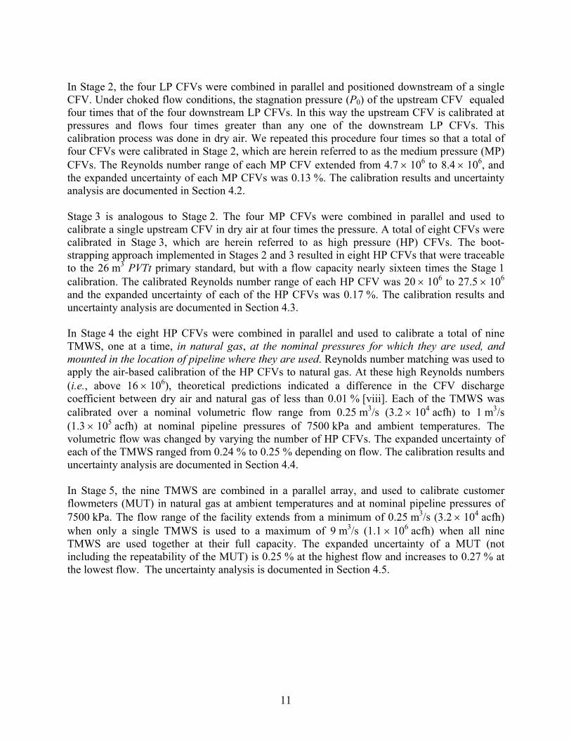
In Stage 2, the four LP CFVs were combined in parallel and positioned downstream of a single CFV. Under choked flow conditions, the stagnation pressure (P0) of the upstream CFV equaled four times that of the four downstream LP CFVs. In this way the upstream CFV is calibrated at pressures and flows four times greater than any one of the downstream LP CFVs. This calibration process was done in dry air. We repeated this procedure four times so that a total of four CFVs were calibrated in Stage 2, which are herein referred to as the medium pressure (MP) CFVs. The Reynolds number range of each MP CFV extended from 4.7 × 106 to 8.4 × 106, and the expanded uncertainty of each MP CFVs was 0.13 %. The calibration results and uncertainty analysis are documented in Section 4.2. Stage 3 is analogous to Stage 2. The four MP CFVs were combined in parallel and used to calibrate a single upstream CFV in dry air at four times the pressure. A total of eight CFVs were calibrated in Stage 3, which are herein referred to as high pressure (HP) CFVs. The boot-strapping approach implemented in Stages 2 and 3 resulted in eight HP CFVs that were traceable to the 26 m3 PVTt primary standard, but with a flow capacity nearly sixteen times the Stage 1 calibration. The calibrated Reynolds number range of each HP CFV was 20 × 106 to 27.5 × 106 and the expanded uncertainty of each of the HP CFVs was 0.17 %. The calibration results and uncertainty analysis are documented in Section 4.3. In Stage 4 the eight HP CFVs were combined in parallel and used to calibrate a total of nine TMWS, one at a time, in natural gas, at the nominal pressures for which they are used, and mounted in the location of pipeline where they are used. Reynolds number matching was used to apply the air-based calibration of the HP CFVs to natural gas. At these high Reynolds numbers (i.e., above 16 × 106), theoretical predictions indicated a difference in the CFV discharge coefficient between dry air and natural gas of less than 0.01 % [viii]. Each of the TMWS was calibrated over a nominal volumetric flow range from 0.25 m3/s (3.2 × 104 acfh) to 1 m3/s (1.3 × 105 acfh) at nominal pipeline pressures of 7500 kPa and ambient temperatures. The volumetric flow was changed by varying the number of HP CFVs. The expanded uncertainty of each of the TMWS ranged from 0.24 % to 0.25 % depending on flow. The calibration results and uncertainty analysis are documented in Section 4.4. In Stage 5, the nine TMWS are combined in a parallel array, and used to calibrate customer flowmeters (MUT) in natural gas at ambient temperatures and at nominal pipeline pressures of 7500 kPa. The flow range of the facility extends from a minimum of 0.25 m3/s (3.2 × 104 acfh) when only a single TMWS is used to a maximum of 9 m3/s (1.1 × 106 acfh) when all nine TMWS are used together at their full capacity. The expanded uncertainty of a MUT (not including the repeatability of the MUT) is 0.25 % at the highest flow and increases to 0.27 % at the lowest flow. The uncertainty analysis is documented in Section 4.5.

12

Figure 3.2 Four Photographs showing the CFVs with end caps and three different size nozzle fixtures Figure 3.2 shows four photographs that include (A) the single aperture nozzle fixture used in Stage 1 to calibrate the LP CFVs; (B) the four LP CFVs with end caps (C) the four aperture nozzle fixture used both in Stage 2 to hold the four LP CFVs and again in Stage 3 to hold the four MP CFVs, and (D) the twenty-one aperture nozzle fixture used in Stage 4 to calibrate the nine TMWS. In Stage 4, the maximum flow was obtained with the HP CFVs mounted in only eight of the possible twenty-one apertures. Additional apertures (which allow for higher flows in the future) were not used. The unused apertures remain sealed for the entire calibration process. The end caps shown in Fig. 3.2 A, B, and D manually screw onto the downstream end of the CFVs to prevent flow. The end caps were used in the Stage 4 calibration of the TMWS using the eight HP CFVs. Initially, two of the eight HP CFVs were uncapped. The remaining six were systematically uncapped to change the volumetric flow through the TMWS being calibrated. The apertures on the face of the nozzle fixtures in Fig. 3.2 A, C, and D, were dimensioned so that once the CFVs were installed they are both sealed and held in place by friction. When the nozzle fixture (with CFVs installed) was mounted in the pipeline, the pressure gradient necessary to choke the CFVs also added to the integrity of the seal. An illustration of the single CFV nozzle fixture installed in the appropriate sized pipeline is shown in Fig. 3.3. This figure corresponds to the Stage 1 calibration setup of the LP CFVs.

13

Flow Direction

Pressure

Temperature Single LP CFV installed in nozzle fixture

10.16 cm20.32 cm

Flow DirectionFlow Direction

PressurePressure

Temperature Single LP CFV installed in nozzle fixture

10.16 cm20.32 cm

Figure 3.3. Stage 1 Calibration setup for LP CFVs

3.2 Description of CFVs and their Calibration Parameters The LP, MP, and HP CFVs used to bootstrap between NIST low pressure, low air flow standard and pipeline scale flows of natural gas were designed according to the ISO 9300 standard [ix]. These flowmeters were selected because of their excellent reproducibility, simple geometric design, straightforward application, and well understood physics. The two dimensionless calibration parameters relevant for CFVs are the discharge coefficient ( dC ) and the Reynolds number ( Re ). The discharge coefficient is a ratio of the actual mass flow ( m& ) to the theoretical mass flow ( thm& ) based on one-dimensional isentropic conditions. The theoretical mass flow is [x]

0u

02

th 4 TRCPdm s Mπ

=& (3.1)

and the discharge coefficient is

Ms02

0u

thd

4=≡

CPdπ

TRmmm

C&

&

& (3.2)

where 0P is the stagnation pressure, 0T is the stagnation temperature, uR is the universal gas constant, M is the molecular weight, d is the throat diameter, and sC is the critical flow function. Appendix A explains how 0P , 0T , and sC are calculated in this work. The Reynolds number definition used herein is

0u0

s0

0

th =4

≡TRμ

CdPdμπ

mRe

M&, (3.3)

where 0μ is the dynamic viscosity evaluated at 0P , 0T . All thermodynamic properties are computed using the REFPROP 8.0 Thermodynamic Database [ii]. The calibration results for Stages 1 through 3 are expressed by plots of dC versus Re . Table 3.1 lists the throat diameters of the four LP CFVs ( LPd ), the four MP CFVs ( MPd ), and the eight HP CFVs ( HPd ) referenced by their serial numbers. The throat diameters of the four LP CFVs were measured to tolerances better than 0.001 mm at a 95 % confidence level by the

14

Precision Engineering Division at NIST. The use of highly accurate d values cause the calibration data for the four LP CFVs to collapse onto a single curve that follows trends predicted by theoretical CFV models [xixii - xiii]. The throat diameters of the MP and HP CFVs are defined so that the MP CFVs and the HP CFVs can be characterized by a single calibration curve that is consistent with the LP CFVs and with theory.

Table 3.1. LP CFVs measured d values and MP and HP CFVs estimated d values.

Total No. of CFVs

LP CFVs

LPd (mm)

MP CFVs

MPd (mm)

HP CFVs

HPd (mm)

1 #2 25.3932 #10 25.3944 #1 25.4123 2 #3 25.3910 #11 25.3952 #7 25.3822 3 #4 25.3935 #12 25.3959 #8 25.3804 4 #5 25.3883 #13 25.3854 #14 25.3958 5 N/A N/A N/A N/A #15 25.3870 6 N/A N/A N/A N/A #17 25.3789 7 N/A N/A N/A N/A #19 25.3921 8 N/A N/A N/A N/A #20 25.4006

3.3 Summary of the Uncertainty of the Five Stage Calibration Process The uncertainty of the five stage traceability scheme is determined using the GUM procedure [xiv]. The uncertainty for each of the five stages is summarized in the bar graph shown in Fig. 3.4. The height of each of the rectangles depicts the standard uncertainty (i.e., k = 1) of the stage it represents. The sum of all five rectangles is 100 % and the root-sum-square of the standard uncertainties multiplied by a coverage factor of two is the expanded uncertainty (i.e., k = 2) of the MUT. For flows ranging from 0.25 m3/s to 9 m3/s (at a nominal pressure of 7500 kPa and at ambient temperatures) the expanded uncertainty varies from 0.27 % to 0.25 %, decreasing with increasing flow.

0

10

20

30

40

50

Stage 1 Stage 2 Stage 3 Stage 4 Stage 5

0.049 %0.041 %

0.051 %

0.082 %

0.051 %

P, T, & misc

NIST Flow Std.K-factor Reprod.

CFV cross-talkCFV species effects

% C

ontr

ibut

ion

to U

ncer

tain

ty

0

10

20

30

40

50

Stage 1 Stage 2 Stage 3 Stage 4 Stage 5Stage 1 Stage 2 Stage 3 Stage 4 Stage 5

0.049 %0.041 %

0.051 %

0.082 %

0.051 %

P, T, & misc

NIST Flow Std.K-factor Reprod.

CFV cross-talkCFV species effects

% C

ontr

ibut

ion

to U

ncer

tain

ty

Figure 3.4. The standard uncertainty and the percent contribution to the total uncertainty of each stage for

MUTq = 2.25 m3/s. (The height of each rectangle indicates the uncertainty contribution in percent for the corresponding stage.)

15

The legend in Fig. 3.4 shows the five different shading patterns used in the bar graph. The three lined shading patterns (i.e., , , ) denote uncertainty components that NIST plans to reduce in the near future. These include the uncertainty introduced in Stage 1 corresponding to the NIST flow standard ( ), the uncertainty introduced in Stage 4 attributed to the reproducibility of the TMWS K-factors ( ), and the uncertainty introduced in Stages 2, 3, and 4 attributed to cross-talk (i.e., interference effects) between the CFVs mounted in a common plenum ( ). The CFV interference effects will be reduced by increasing the spacing between the CFVs used in parallel. The K-factor reproducibility is currently based on only two calibrations. We anticipate lower values in the future as repeated calibrations provide a larger data set to more accurately determine the long term random effects and flowmeter drift. Lastly, NIST is currently working to reduce the uncertainty of the NIST flow standard used in Stage 1. The two solid shading patterns (i.e., and ) in Stages 2, 3, 4, and 5 include multiple uncertainty sources that have been grouped together. The first pattern of solid shading ( ) includes uncertainty components attributed to pressure and temperature measurements, line pack effects, and various other sources. A detailed listing of the individual uncertainty components contained in these groupings is included in Section 4 and in references [xv, xvi]. The second pattern of solid shading ( ) is attributed to CFV species effects. CFV species effects include uncertainty contributions from the following four thermodynamic properties: sC for air in Stage 3, and sC , Z , and M for natural gas in Stage 4. The cause of this uncertainty is twofold. First, the uncertainty attributed to sC in Stages 3 and 4 is a consequence of calibrating the HP CFVs in air, but applying the calibration to natural gas. Second, the Stage 4 uncertainty attributed to Z and M results because the density of the natural gas is required to convert from the mass flow predicted by the HP CFVs to volumetric flow needed for the TMWS calibration. The uncertainties of these parameters are already nearly optimized, and are not likely to be reduced in the near future. 4. CALIBRATION ANALYSIS OF THE FIVE STAGE TRACEABILITY PROCESS This section provides a detailed analysis of the calibration results and uncertainty for each of the five stages used to establish traceability to NIST. The governing calibration equations are developed for each of the five stages. The uncertainty introduced by each stage is determined using the method of propagation of uncertainty [xvii]. The GUM procedure [xviii] is followed whereby uncertainty sources are categorized as either Type A (i.e., those which are evaluated by statistical methods) or Type B (i.e., those which are evaluated by other means). Uncertainties having subcomponents belonging to both Type A and Type B are categorized as (A, B). The uncertainty analysis accounts for correlated uncertainty sources within and between each of the five stages. In all five stages the flow properties (e.g., the critical flow function, density, viscosity, etc.) are calculated using the REFPROP 8 Thermodynamic Database [ii]. In the first three stages the working fluid is air. The mole fraction of water vapor is maintained below 4.1 × 10-5 so that the air can be considered to be dry air. However, effects of water vapor are considered in the uncertainty budget. Table 4.1 shows the composition of dry air used to calculate flow properties in this work. The air composition is the average value of multiple references [xix - xxxxi].

16

Table 4.1 Composition of air used in Stages 1 through 3

Species Mole Fraction (%) Nitrogen 78.0849 Oxygen 20.9478 Argon 0.934

Carbon Dioxide 0.0314

4.1 STAGE 1: Calibration and Uncertainty of LP CFVs

Calibration of the LP CFVs In Stage 1, NIST’s 26 m3 PVTt primary flow standard was used to calibrate the four LP CFVs in dry air. The PVTt flow standard uses a timed collection technique to determine the LP CFV mass flow. The flow emanating from the LP CFV was diverted from the bypass into the nearly evacuated collection tank for a measured time interval. The average gas temperature and pressure in the collection tank as well as in the inventory volume were measured before and after the filling process. These measurements were used in conjunction with the REFPROP 8 Thermodynamic Database [ii] to determine the initial and final densities of the gas in the collection tank ( i

Tρ and fTρ ), and in the inventory volume ( i

Iρ and fIρ ). In the absence of leaks,

the time averaged mass flow equals the change in mass within the collection tank (i.e., gas density change in the collection tank multiplied by the collection tank volume) plus the change in mass in the inventory volume (i.e., gas density change in the inventory volume multiplied by the inventory tank volume) divided by the collection time

tVVm

Δ-- I

iI

fIT

iT

fT )()( ρρρρ +

=& (4.1)

where TV is the collection tank volume; IV is the inventory volume; and tΔ is the collection time interval. The standard relative uncertainty of PVTt mass flow measurements is

( )[ ]mmu && = 0.045 %. A detailed description of the PVTt system and its uncertainty can be found in references [v-vii].

VacuumExhaustValve

LP CFV

TankInlet

Valve CollectionTank

Bypass

Fan

FanDuct

BypassValve

Steady FlowSource

InventoryVolume

Tm P

VacuumExhaustValve

LP CFV

TankInlet

Valve CollectionTank

Bypass

Fan

FanDuct

BypassValve

Steady FlowSource

InventoryVolume

Tm P

Figure 4.1. Schematic of NIST 26 m3 PVTt Primary Flow Standard

17

The mass flows measured by the PVTt flow standard were used to calculate dC values for each of the four LP CFVs using Eqn. 3.2, while the Reynolds number was computed using Eqn. 3.3. Figure 4.2 shows the calibration data for all four LP CFVs plotted on a logarithmic Reynolds number axis. Included in the figure are the results for the MP and HP CFVs. These results are plotted along with the LP CFV data so that general trends for all three stages of CFV calibration data (i.e., Stages 1, 2, and 3) can be easily observed. The MP and HP CFV data, however, are not discussed in this section, but are covered in Sections 4.2 and Sections 4.3, respectively. The LP CFV data shown in the figure incorporate two different PVTt calibrations, the first in 2004, and the second two years later in 2006. In both sets of calibration data the four LP CFVs are depicted by triangles having four different orientations. Open triangles are used for the 2004 dataset (i.e., - CFV #2; - CFV #3; - CFV #4; - CFV #5) while closed triangles are used for the 2006 data set (i.e., - CFV #2; - CFV #3; - CFV #4; - CFV #5). For clarity, this nomenclature is also denoted in the legend of Fig. 4.2. Each data point in the figure is the average of a minimum of four repeated PVTt flow measurements at the same nominal flow. In general, the standard deviation of the four (or more in some cases) repeated flow measurements is 0.006 %.

0.991

0.992

0.993

0.994

0.995

0.996

0.997

Re

Cd

105 106 107 108

0.1 %Stage 3HP CFV

Data

Stage 2MP CFV

Data

MP & HP CFVCurve Fit

LP CFVCurve Fit

TurbulentFlow

CFV Theory

2004 2006LP CFVs#2

#4#5

#3

Laminar FlowCFV Theory

0.998

Stage 1LP CFVcore Re

range

0.991

0.992

0.993

0.994

0.995

0.996

0.997

Re

Cd

105 106 107 108105 106 107 108

0.1 %0.1 %Stage 3HP CFV

Data

Stage 2MP CFV

Data

MP & HP CFVCurve Fit

LP CFVCurve Fit

TurbulentFlow

CFV Theory

2004 2006LP CFVs 2004 2006LP CFVs#2#2

#4#5#5

#3#3

Laminar FlowCFV Theory

0.998

Stage 1LP CFVcore Re

range

Figure 4.2. Calibration data for the LP, MP, and HP CFVs.

The theoretical dC values for the laminar CFV flow model ( ) [viii] and the turbulent CFV flow model ( ) [viii] are plotted with the calibration data in Fig. 4.2 to clearly illustrate that

18

the LP CFV results lie almost entirely in the transitional flow regime. As expected, the portion of the calibration data below 610<Re closely follows the laminar flow model. However, at higher Reynolds numbers the data falls slightly below the turbulent flow model. The apparent discrepancy at higher Reynolds numbers could be the result of the flow not being fully turbulent. In any circumstance the difference (i.e., less than 0.1 %) is well within expected capability of the turbulent flow model.

In total, the LP CFV results include 95 data points that span a Reynolds number range from 6.5 × 105 to 2.8 ×106. However, only CFV #3 and CFV #5 were calibrated over this extended Reynolds number range. The core Reynolds number range for which all four LP CFVs were calibrated extends from 1.1 × 106 to 2.4 × 106, corresponding to stagnation pressures ranging from 350 kPa to 700 kPa at ambient temperatures. The data within the core Reynolds number range is used in Stage 2 when the array of LP CFVs are used to calibrate the MP CFVs. The Reynolds numbers values outside this core region were obtained primarily to ensure that the data followed the expected theoretical trends in the laminar and turbulent flow regimes. Within the core region, dC values were measured at no less than 11 equally spaced Re to capture the changes in concavity that occur in the transitional flow regime. Considering that the core data includes four different LP CFVs, each calibrated twice two years apart, and that the data lies entirely in the transitional flow regime, the tight overlap between the data is remarkable. As indicated in the figure, the data in the core region for all four LP CFVs can be represented by a single calibration curve

52-2

51-10d, ++=LP

FIT RebRebbC

(4.2)

where the coefficients 0b , 1b , and 2b are given in Table 4.2, and the standard deviation of the curve fit residuals is 0.018%. The same polynomial expression is used to fit the calibration data for the MP and HP CFVs, and their curve fit coefficients are also included in Table 4.2. Lastly, the curve fits shown in Fig. 4.2 agree to better than 0.05 % with data from PTB (flowing air at low flows and natural gas at high flows) and with LADG-LNE (flowing air) [xxii ]. This comparison was done using the following nozzles, CFV #2, CFV #3, CFV #4, and CFV #5.

Table 4.2. Calibration Coefficients for LP, MP, and HP CFVs and the Reynolds number range where the fit is valid.

CFV ReMIN ReMAX b0 b1 b2

(-----) (-----) (-----) (-----) (-----) (-----)

LP CFVs 1.1 × 106 2.4 × 106 1.101 -3.917 35.683

MP CFVs 3.69 × 106 2.74 × 107 1.0003 -0.1323 0

HP CFVs 3.69 × 106 2.74 × 107 1.0003 -0.1323 0

19

Uncertainty Analysis of the LP CFVs When the method of propagation of uncertainty is applied to Eqn. 3.2 (i.e., the calibration equation used for the LP CFVs in Stage 1) the result is2

( ) ( ) ( ) ( ) 2

0

02

0

022

d

d

LP1LP1LP1 41

⎥⎦

⎤⎢⎣

⎡+⎥

⎦

⎤⎢⎣

⎡+⎥⎦

⎤⎢⎣⎡=⎥

⎦

⎤⎢⎣

⎡TTu

PPu

mmu

CCu

&

& ( ) 2

LP14 ⎥⎦

⎤⎢⎣⎡+

ddu ( ) 2

LP141

⎥⎦⎤

⎢⎣⎡+

MMu

( ) 2

u

u41

⎥⎦

⎤⎢⎣

⎡+

RRu ( ) 2

s

s

LP1⎥⎦

⎤⎢⎣

⎡+

CCu ( ) 2

d

d

LPFIT

FIT

⎥⎥⎦

⎤

⎢⎢⎣

⎡+

C

Cu

(4.3)

where the subscript “LP1” indicates the Stage 1 LP CFVs, and ][ FITFITdd )( CCu is the standard

deviation of the curve fit residuals. In this expression, the correlations of sC with 0P and 0T have been neglected. In a more exact representation the normalized sensitivity coefficients of 0P and 0T would include the appropriate pressure and temperature derivatives of sC . However, a sensitivity study showed that these dependencies could be omitted with negligible error in both Stages 1 and 2 where the pressure is sufficiently low. On the other hand, we include these dependencies in the uncertainty expressions in Stages 3, 4, and 5 where the pressure is substantially higher. Furthermore, the correlation between 0P and 0T (through their common dependence on the specific heat ratio, γ , and on the Mach number, M , [see Eqns. A1 and Eqn. A2 in Appendix A]) affects the uncertainty budget by less than 1 × 10-6 and is ignored.

Table 4.3. Stage 1 Uncertainty Budget for the LP CFV Discharge Coefficient

Unc. Components for Stage 1 LP CFVs Rel. Unc. (k=1)

Sen. Coeff.

Perc. Contrib.

Unc. Type

Comments

LP CFV Discharge Coeff., Cd = 0.9936 (× 10-6) (-----) (%) (A or B)

PVTt primary standard, ( m& = 675.2 g/s) 450 1.0 79.9 A, B Based on References [v - vii]

Stag. Pres.; (P0 = 570.0 kPa) 118 1.0 5.5 A, B Fit residuals, drift, cal std, etc.

Stag. Temp.; (T0 = 296.0 K) 176 0.5 3.1 A, B Spatial Sampling error, drift, fit residuals, etc .

Nominal Throat diameter; (d = 2.54 cm) 0* 2.0 0 B Nom. value is fixed betwn. Stages 1 and 2

Molar Mass; (M = 28.9646 g/mol) 25 0.5 0.1 A, B Variation in air comp. [xix-xxi]

Univ. gas constant; (Ru = 8314.47 J/kmol K) 2 0.5 0.0 A, B See Reference [xxiii]

Critical Flow Function; ( LPs,C =0.6865 ) 0* 1.0 0 B Same flow cond. in Stages 1 and 2

CFV Curve Fit Residuals 170 1.0 11.4 A Fit Residuals, Hysteresis, and Reproducibility

Combined Uncertainty 503 100

2 For convenience, all uncertainty formulas give the square of the actual value unless otherwise noted.

20

Based on Eqn. 4.3, the Stage 1 uncertainty for the discharge coefficient was 0.05 % with a coverage factor of k = 1. The various uncertainty sources are itemized in Table 4.3. The abbreviated titles in the heading of the table, “Rel. Unc.”, “Sen. Coeff.”, “Perc. Contrib.”, and “Unc. Type”, are taken to mean the following: (1) standard relative uncertainty; (2) normalized sensitivity coefficient; (3) percent contribution of a single component to the overall uncertainty; and (4) the uncertainty type, respectively. By far, the largest component is the relative standard uncertainty of the PVTt primary standard (450 × 10-6). Brief explanations of the remaining uncertainty components are provided in Table 4.3 under the heading “Comments”. Throughout this document an asterisk (*) next to an uncertainty value in the “Rel. Unc.” column is used to indicate self-canceling measurement errors between adjacent stages. In Table 4.3 the asterisk is used next to the uncertainties for the nominal CFV throat diameter and the critical flow function. Both of these uncertainties are self-canceling since biases introduced in Stage 1 identically cancel with biases of opposite polarity in Stage 2. For example, any bias in the value of the throat diameter used in Stage 1 cancels when the same value of d is used in Stage 2. This argument also applies to the critical flow function since the LP CFVs are used in Stage 2 for the same gas type (i.e., dry air) and at the same nominal conditions (i.e., 0P and 0T ) for which they were calibrated in Stage 1. 4.2 STAGE 2: Calibration and Uncertainty of the MP CFVs

Calibration of the MP CFVs using the LP CFVs In Stage 2, the four LP CFVs calibrated in Stage 1 are combined in a parallel array and used to calibrate four MP CFVs, one at a time. The calibration setup is shown in Fig. 4.3. Both the downstream LP CFVs and the upstream MP CFV have a CPA 50E flow conditioner3 installed upstream of their respective pressure and temperature instrumentation. A heat exchanger is used to bring the cold jet exiting the MP CFV back to room temperature conditions before the flow is measured by the array of LP CFVs.

Du = 15.24 cm

Heat Exchanger

PTm

Tm P

CPA 50E FlowConditioner

CPA 50E FlowConditioner LP CFVs

MP CFVDirection

Flow

Dd = 30.48 cm

Du = 15.24 cm

Heat Exchanger

Heat Exchanger

PPPTmTmTmTm

TmTmTm PP

CPA 50E FlowConditioner

CPA 50E FlowConditioner LP CFVs

MP CFVDirection

Flow

Direction

Flow

Dd = 30.48 cm

Figure 4.3. Schematic showing the setup for the Stage 2 calibration of the MP CFV using four LP CFVs calibrated

in Stage 1 (figure not drawn to scale)

3 Throughout this document certain commercial equipment, instruments, or materials are identified to foster

understanding. Such identification does not imply recommendation or endorsement by the National Institute of Standards and Technology, nor does it imply that the materials or equipment identified are necessarily the best available for the purpose.

21

The operating conditions for the downstream LP CFVs are controlled so that 0P and 0T are nearly equal to their Stage 1 values. Because the working fluid is the same as that in Stage 1 (i.e., dry air), the resulting Reynolds number range corresponds to the values used in the Stage 1 LP CFV calibration. By applying the principle of conservation of mass and using the LP CFVs as working standards, the mass flow through the upstream MP CFV is

21n

nd,nth, Δ∑2

LPLP2MP2 mCmm

N&&& +=

=

(4.4)

where 42 =N is the number of LP CFVs mounted in the downstream nozzle fixture, and LP2nth,m&

is the Stage 2 theoretical mass flow for the LP CFVs which is calculated using Eqn. 3.1; and 2Δm& is the rate of mass storage in the connecting volume between the array of LP CFVs and the

MP CFV. The mass storage (i.e., line pack) term accounts for density transients in the connecting volume. Because 2Δm& is small relative to MP2m& , we set 2Δm& equal to zero in Eqn. 4.4; however, the uncertainty attributed to line pack is included in the uncertainty budget.

The calibration procedure begins by establishing steady-state flow conditions at the desired stagnation pressure. Subsequently, pressure and temperature data is collected for approximately 360 s. The data acquisition system cycles at 1.5 Hz, resulting in approximately 540 pressure and temperature data points. At each data point 0P , 0T , sC , and Re are computed at both the LP CFVs and at the MP CFV using the methods explained in Section 3.2 and in Appendix A. These values are used to calculate the MP CFV discharge coefficient

∑2

LP

MP

LP

MP2MP2

LP2LP2

LP2

MP2

MP

MP

1nnd,2

2n,

s,0

s,0

0

0

thd ≡

N

,

,

,

, Cdd

CPCP

TT

mmC

=⎟⎟⎠

⎞⎜⎜⎝

⎛⎟⎟⎠

⎞⎜⎜⎝

⎛=⎥

⎦

⎤⎢⎣

⎡&

& (4.5)

where the subscripts “LP2” and “MP2” correspond, respectively, to the Stage 2 LP and MP CFVs. The CFV throat diameters are given in Table 3.1, and )( LP

LPFIT

LPd,nd, ReCC = is the LP CFV

calibration curve given in Eqn. 4.2. The reported MPdC values are averaged over the 360 s data

collection interval. In the worst case, the standard deviation of the mean for this averaging process is 0.002 %, which is negligible relative to other sources of uncertainty, and is therefore not included in the uncertainty budget.

The MPdC values are measured at a minimum of five discrete MPRe values. A minimum of two

MPdC measurements are made at each of the five Reynolds numbers so that a total of no less than

ten measurements are made. A typical calibration begins at the minimum pressure set point, LP20,P =375 kPa (or MP20,P = 1500 kPa). The set point is increased in equal increments until

reaching its maximum value at the fifth pressure set point, LP20,P =630 kPa (or

MP20,P = 2520 kPa). After finishing the fifth data collection, the flow is shutdown (i.e., zero flow) and then reestablished at the maximum set point. The sixth data collection is taken at the maximum set point. The pressure set point is subsequently decreased in equal increments until reaching its minimum value at the tenth set point. This method of collecting data accounts for repeatability, short term reproducibility, and hysteresis effects.

22

The averaged MPdC data is depicted in Fig. 4.2 (shown earlier in Section 4.1) where the symbol

( ) represents the results of all four MP CFVs. This data set includes a total of 77 points and spans a Reynolds number range from 3.7 × 106 to 8.6 × 106. Unlike the LP CFV data, the MP CFV data is entirely within the turbulent flow regime. Moreover, the entire MP CFV data set can be fit to a single calibration curve

51-MPFIT 10d, += RebbC

(4.6)

where the coefficients 0b and 1b are given in Table 4.2. Considering that the data corresponds to five different CFVs, the small degree of scatter in the data is remarkable; moreover, the standard deviation of the curve fit residuals is only 0.017 %. Perhaps more remarkable is the fact that the same curve also fits the eight HP CFVs in Section 4.3.

Uncertainty Analysis of the MP CFVs The uncertainty of the MP CFV discharge coefficients is determined by applying the law of propagation of uncertainty to Eqn. 4.5. Because all four LP CFVs are traceable to the same calibration standard, many of their common uncertainty sources are correlated. When these correlations are taken into account, the resulting expression for uncertainty is

( ) ( ) ( ) 2

d

d

2

22

d

d

LP

LP

MP

1-1⎥⎦

⎤⎢⎣

⎡⎟⎟⎠

⎞⎜⎜⎝

⎛ +=⎥

⎦

⎤⎢⎣

⎡CCu

NNr

CCu ( ) ( ) 2

0

02

0

0

LP2MP2⎥⎦

⎤⎢⎣

⎡+⎥

⎦

⎤⎢⎣

⎡+

PPu

PPu

( ) 2

0

0

MP241

⎥⎦

⎤⎢⎣

⎡+

TTu ( ) 2

0

0

LP241

⎥⎦

⎤⎢⎣

⎡+

TTu ( ) 2

MP24 ⎥⎦

⎤⎢⎣⎡+

ddu ( ) 2

LP24 ⎥⎦

⎤⎢⎣⎡+

ddu

( ) 2

s

s

MP2⎥⎦

⎤⎢⎣

⎡+

CCu ( ) 2

s

s

LP2⎥⎦

⎤⎢⎣

⎡+

CCu ( ) 2

d

d

MPFIT

FIT

⎥⎥⎦

⎤

⎢⎢⎣

⎡+

C

Cu 2IE,2+ u

22

MP2

Δ

⎥⎥⎦

⎤

⎢⎢⎣

⎡+

mm&

&

(4.7)

where LPdd ][ CCu )( in the first term is the uncertainty for a single LP CFV used by itself. Its uncertainty is determined using Eqn. 4.3 and its value is given in Table 4.3. The uncertainty of all four LP CFVs used together is given by the entire first term, including LPdd ][ CCu )( and the

coefficient in parenthesis to which it is multiplied. The coefficient multiplying LPdd ][ CCu )( accounts for the correlation between the four LP CFVs where the correlation coefficient ( LPr ) specifies the degree of correlation. In the hypothetical case when 0=LPr (i.e., no correlated

sources of uncertainty), the coefficient multiplying LPdd ][ CCu )( is 21 N , indicating that the uncertainty of all four LP CFVs used together is less than their individual use. On the other hand, if 1=LPr (i.e., perfectly correlated uncertainty sources), the coefficient multiplying

LPdd ][ CCu )( is unity, and there is no difference in uncertainty between using a single LP CFV or multiple LP CFVs together. In the scope of the current work we expect the correlation coefficient to be close to unity since many of the uncertainty sources are correlated. Using the method outlined in reference [xv], we calculated the correlation coefficient to be 920=LP .r .

23

The last three terms in Eqn. 4.7 are the uncertainties attributed to the standard deviation of the MP CFVs curve fit residuals,

MPFITFIT ][ dd )( CCu ; followed by the uncertainty caused by

interference effects (i.e., cross-talk) between the four downstream LP CFVs, ( 2IE,u ); and lastly the uncertainty attributed to the line packing effect, ][ MP22Δ mm && . The uncertainty attributed to interference effects was measured experimentally by varying the number of open LP CFVs (between two and four) in the nozzle fixture, and comparing the performance to an upstream reference CFV held at constant mass flow. These tests were done on three different occasions and showed that the maximum influence of interference effects was 500 × 10-6. Assuming a rectangular distribution the standard uncertainty attributed to interference effects is 289 × 10-6. The uncertainty attributed to the line packing effect was assessed by multiplying the connecting volume by the average rate of density change (in the connecting volume) during the collection. An itemized list of all the uncertainty components along with brief explanations of their uncertainty values are given in Table 4.4.

Table 4.4. Stage 2 Uncertainty Budget for the MP CFV Discharge Coefficient.

Unc. Components for Stage 2 MP CFVs. Rel. Unc. (k=1)

Sen. Coeff.

Perc. Contrib.

Unc. Type

Comments

MP CFV Discharge Coeff., Cd = 0.9936 (× 10-6) (-----) (%) (A or B) Discharge Coeff. For array of 4 LP CFVs, ( LP

dC = 0.9936) 487 1 57.6 A, B Stage 1 calibration (Corr. effects included)

MP Stag. Pres.; (P0 = 2280 kPa) 125* 1 3.7 A, B Uncorr. Unc.: Random Effects, Data Acq., Barometric. Pres.

LP Stag. Pres.; (P0 = 570 kPa) 129 1 3.9 A, B Cal. Std., Random Effects, Data Acq., Barometric Pres.

MP Stag. Temp.; (T0 = 295 K) 230 0.5 3.1 A, B Cal. Std., Random Effects., Spatial Non-uniformity, etc.

LP Stag. Temp.; (T0 = 291 K) 241 0.5 3.5 A, B Cal. Std., Random Effects., Spatial Non-uniformity, etc.

MP Critical Flow Function; ( MPs,C = 0.6912) 0* 1 0 A,B Perfectly correlated betwn. Stages 2 and 3

LP Critical Flow Function; ( LPs,C = 0.6865) 0* 1 0 A,B Perfectly correlated betwn. Stages 1 and 2

Nominal Diameter MP CFV, (d = 2.54 cm) 0* 2 0 B Perfectly correlated betwn. Stages 2 and 3

Nominal Diameter LP CFV, (d = 2.54 cm) 49* 2 2.3 B Unc. for thermal expansion betwn. Stages 1 and 2

LP CFV Curve Fit Residuals 170 1 6.9 A Std. Dev. of Curve Fit Residuals, (see Section 4.1)

Interference effects of multiple CFVs in a Common Plenum 289 1 19.8 B Exp. varying number of open

CFVs in nozzle fixture

Line pack effect 27 1 0.2 B Based on measured dtρVd in connecting volume during cal.

Combined Uncertainty 648 100 When the uncertainties listed in Table 4.4 are used in Eqn. 4.7 the relative standard uncertainty for MP

dC is 648 ×10-6 (k = 1). As expected, the largest uncertainty contribution derives from the

24

Stage 1 calibration of the four LP CFVs. The value for this uncertainty (487 × 10-6) is slightly less than that given in Table 4.3 for the Stage 1 analysis because 1<LPr . As discussed in Section 4.1, the asterisk (*) next to selected uncertainty components indicates our assumption that the correlated measurement errors between adjacent stages identically cancel. In the cases where an asterisk is positioned next to the pressure or temperature uncertainties the correlation is caused by the same transducer being used to measure the same nominal conditions in adjacent stages. In this case the listed uncertainties consist entirely of the uncorrelated uncertainty sources. When there is ambiguity as to whether an uncertainty source is perfectly correlated, we conservatively define it to be uncorrelated. 4.3 STAGE 3: Calibration and Uncertainty of the HP CFVs

Calibration of the HP CFVs In Stage 3 the MP CFVs are configured in parallel and used to calibrate a total of eight HP CFVs, one at a time, in dry air. The calibration setup is similar to the Stage 2 setup shown in Fig. 4.3, but in this case a single HP CFV is positioned upstream of the four MP CFVs configured in parallel. The Stage 3 stagnation pressure at the MP CFVs is controlled so that the Reynolds number overlaps values from the previous calibration stage. The resulting Reynolds number range for the MP CFVs varies from 5.4 × 106 to 7.5 × 106, and the Reynolds number range for the upstream HP CFV varies from 2.0 × 107 to 2.75 × 107. The pressures and flows of the HP CFVs are approximately 16 times the Stage 1 values for the LP CFVs. The calibration procedure is similar to the calibration of the MP CFVs. After establishing steady state flow conditions in the pipeline, data is collected for approximately 200 s resulting in approximately 270 data points. At each data point we compute 0P , 0T , sC , and Re at the MP CFVs and at the HP CFV using the methods described in Section 3.1. These values are used to calculate the HP CFV discharge coefficient

∑3

MP

HP3

MP3

HP3HP3

P3MP3

MP3

HP3

HP

HP

1nd,2

2n,

s,0

Ms,0

0

0

thd m

m≡N

n,

,

,

, Cd

dCPCP

TT

C=

⎟⎟⎠

⎞⎜⎜⎝

⎛⎟⎟⎠

⎞⎜⎜⎝

⎛=⎥

⎦

⎤⎢⎣

⎡&

& (4.8)

where the subscripts “MP3” and “HP3” correspond, respectively, to the Stage 3 MP and HP CFVs, and 4=3N is the number of MP CFVs mounted in the downstream nozzle fixture. The throat diameters of the CFVs are obtained from Table 3.1, and )( MP

MPFIT

MPd,nd, ReCC = is the MP

CFV calibration curve given by Eqn. 4.6. The reported HPdC values are averaged over the 200 s

data collection interval. The averaging process introduces negligible uncertainty since in the worst case, the standard deviation of the mean is less than 0.001 %.

For each HP CFV, HPdC measurements are made at a minimum of three discrete HPRe values. In

most cases these measurements were made on two separate occasions so that six measurements are made in total. The format for collecting the data is analogous to the procedure described in Section 4.2. The entire data set for all eight HP CFVs consists of 43 points. The data is shown in Fig. 4.2 (shown earlier in Section 4.1) where the same symbol ( ) is used to represent all eight HP CFVs. The eight HP CFVs fit a single calibration curve

25

51-HPFIT 10d, RebbC +=

(4.9)

where the coefficients 0b and 1b are given in Table 4.2, and the standard deviation of the curve fit residuals is 0.02%.

Uncertainty Analysis of the HP CFVs The uncertainty of the HP CFVs is determined by applying the method of propagation of uncertainty to Eqn. 4.8. The resulting expression of uncertainty is analogous to Eqn. 4.7 for the MP CFVs

( )=⎥

⎦

⎤⎢⎣

⎡2

d

d

HPCCu ( ) ( ) 2

nd,

nd,

3

3

MP

MP 1-1

⎥⎥⎦

⎤

⎢⎢⎣

⎡⎟⎟⎠

⎞⎜⎜⎝

⎛ +

CCu

NNr ( ) 2

0

02

0

s

s

0

HP3HP3∂∂1 ⎥

⎦

⎤⎢⎣

⎡

⎥⎥⎦

⎤

⎢⎢⎣

⎡⎟⎟⎠

⎞⎜⎜⎝

⎛++

PPu

PC

CP

( ) 2

0

02

0

s

s

0

HP3HP3∂∂-

21

⎥⎦

⎤⎢⎣

⎡⎥⎦

⎤⎢⎣

⎡⎟⎟⎠

⎞⎜⎜⎝

⎛+

TTu

TC

CT ( ) 2

0

0

MP3⎥⎦

⎤⎢⎣

⎡+

PPu ( ) 2

0

0

MP341

⎥⎦

⎤⎢⎣

⎡+

TTu

( ) 2

s

s

HP3⎥⎦

⎤⎢⎣

⎡+

CCu ( ) 2

s

s

MP3⎥⎦

⎤⎢⎣

⎡+

CCu ( ) 2

HP34 ⎥⎦

⎤⎢⎣⎡+

ddu ( ) 2

MP34 ⎥⎦

⎤⎢⎣⎡+

ddu

( ) 2

d

d

MPFIT

FIT

⎥⎥⎦

⎤

⎢⎢⎣

⎡+

C

Cu 2IE,3+ u

23

HP

Δ⎥⎦

⎤⎢⎣

⎡+

mm&

&

(4.10)

where in this case the MP CFV correlation coefficient is MPr = 0.95. The normalized sensitivity coefficients for HP00 )( ][ PPu and HP00 )( ][ TTu include the pressure and temperature derivatives of sC , respectively. These additional terms take into account the uncertainty in sC attributed to uncertainties in the stagnation conditions. At the lower pressures in Stages 1 and 2 these additional terms made a negligible contribution to the uncertainty and were omitted. However, at the elevated pressures in Stages 3 through 5 they are not negligible and are therefore included.

26

Table 4.5. Stage 3 Uncertainty Budget for the HP CFV Discharge Coefficient.

Unc. Components for Stage 3 HP CFVs. Rel. Unc. (k=1)

Sen. Coeff.

Perc. Contrib.

Unc. Type

Comments

HP CFV Discharge Coeff., Cd = 0.9960 (× 10-6) (-----) (%) (A or B) Discharge Coeff. For array of 4 MP CFVs, ( MP

dC = 0.9947) 635 1 56.4 A, B Stage 2 calibration (Corr. effects included)

HP Stag. Pres.; (P0 = 9120 kPa) 279 1.03 11.6 A, B Pres. Cal. Std., Random Effects, Data Acq., Barometric. Pres.

MP Stag. Pres.; (P0 = 2280 kPa) 123* 1 2.1 A, B Uncorr. Unc: Random Effects, Data Acq., Barometric Pres. (Corr. Unc. are self-canceling)

HP Stag. Temp.; (T0 = 295 K) 238 0.64 3.2 A, B See Reference [xv] (Corr. Unc. are self-canceling)

MP Stag. Temp.; (T0 = 290 K) 234* 0.5 1.9 A, B See Reference [xv] (Corr. Unc. are self-canceling)

HP Critical Flow Function; ( HPs,C = 0.7097) 215 1 5.8 A,B Comp. of four Therm. Databases [ii, xxiv - xxvxxvi]

MP Critical Flow Function; ( MPs,C = 0.6916) 0* 1 0 A,B Perfectly correlated betwn. Stages 2 and 3

Nominal Diameter HP CFV, (d = 2.54 cm) 0* 2 0 B Perfectly correlated betwn. Stages 3 and 4

Nominal Diameter MP CFV, (d = 2.54 cm) 49* 2 1.4 B Unc. for thermal expansion betwn. Stages 1 and 2

MP CFV Curve Fit Residuals 200 1 5.6 A Std. Dev. of Curve Fit Residuals, (see Section 4.2)

Interference effects of multiple CFVs in a Common Plenum 289 1 11.7 B See Section 4.2

Line pack effect 44 1 0.3 B Based on measured dtρVd in connecting volume during cal.

Combined Uncertainty 849 100 4.4 STAGE 4: Calibration and Uncertainty of the TMWS

Calibration of the TMWS In Stage 4 all nine TMWS were individually calibrated in natural gas at their place of use and at their nominal operating conditions. Each TMWS was calibrated against the HP CFVs that were calibrated in air in Stage 3. The air based calibration can be applied to nozzles flowing natural gas by accounting for real gas effects via the critical flow function, and by matching the Reynolds number. At these high Reynolds numbers (i.e., Re > 16 x 106) turbulent CFV theory predicts that the difference between the dC values for air and natural gas are less than 0.01 % [xxii]. Because the viscosity of natural gas is less than dry air, matching the Reynolds number required that 0P in the natural gas flow be approximately 20 % lower than its value in dry air. During the calibration process the HP CFVs were maintained below their measured choking pressure ratio (i.e., pressure downstream of the HP CFVs divided by the stagnation pressure) of 0.942.

27

Du = 30.48 cm

Dd = 76.2 cm

FlowConditioner HP CFV

Array

TMWS

P

f

T

Tm1

Tm2P

UltrasonicFlowmeter

Body

Ts

Flow Direction

Du = 30.48 cm

Dd = 76.2 cm

FlowConditioner HP CFV

Array

TMWS

P

f

T

Tm1

Tm2P

UltrasonicFlowmeter

Body

Ts

Flow Direction

Figure 4.4. Schematic showing the setup for the Stage 4 calibration of the TMWS using the array of HP CFVs

calibrated in Stage 3 (not drawn to scale) The TMWS were calibrated twice, once in May 2006, and again in June 2007. A schematic of the calibration setup is shown in Fig 4.4 including the auxiliary pressure, temperature, and frequency measurements. For both tests, redundant instrumentation was used to measure frequency and pressure at the TMWS, and averaged values were used for these two measurements. The temperature at the TMWS was measured with a single resistance temperature device (RTD) installed in a thermowell. Pre-calibration tests showed the maximum effect of the thermowell on the measured temperature was 50.8 mK (0.017 %). A flow conditioner was installed downstream of the TMWS just before the array of HP CFVs. The conditioner was used to reduce jetting effects as the flow transitions from the smaller 30.48 cm (12 inch) diameter pipeline to the larger 76.2 cm (30 inch) diameter pipeline. Just downstream of the flow conditioner the first temperature measurement (i.e., m1T in Fig. 4.4) was made by averaging the readings of 10 RTDs spaced at equal distances around the circumference of the pipe. The lengths of the RTDs vary so that their penetration depth into the flow stream ranged from 5 cm (i.e., near the pipe wall) to 36 cm (i.e., near the pipe centerline). In this way the temperature was sampled at multiple radii across the cross section. The uncertainty attributed to temperature variation within the cross section was taken to be the standard deviation of the 10 RTDs. Two pipe diameters ( dD ) downstream, just before the array of HP CFVs, a second temperature measurement was made (i.e., m2T in Fig. 4.4) using 10 RTDs evenly distributed around the circumference of the pipeline. None of the RTDs at either cross section were installed in thermowells. Figure 4.5 includes four pictures showing the flow conditioner (A); the calibration setup (B); the 10 RTDs used to measure m2T (C); and the HP CFV array (D). The eight HP CFVs calibrated in Stage 3 were installed in the twenty-one aperture nozzle fixture. The nozzle fixture was installed in the pipeline that houses an ultrasonic flowmeter. Although the ultrasonic flowmeter was not used in the current work it can provide additional temperature information in the future if necessary. To this point, all temperature information was determined using the RTDs. For the May 2006 test only the 10 RTDs that measure m1T were used. The second set of 10 RTDs used to measure m2T were added for the June 2007 tests to determine the uncertainty attributed to axial temperature gradients. The static pressure instrumentation (not shown in Fig. 4.5B) was located approximately one diameter upstream of the HP CFVs on the bottom of the pipe.

28

Equations 3.1 and 3.2 in Appendix A were used to calculate the stagnation pressure and temperature, respectively.

Flow Direction

HP CFVNozzle Fixture

Tm1Tm2

Location ofFlow Conditioner

(Viewed from Downstream) (Viewed from Downstream)

Flow Conditioner

10 RTD’s used to Measure Tm2 HP CFV Array Installed in Pipeline

A B

C D

(Viewed from Upstream)

HP CFV Array Setup

Flow Direction

HP CFVNozzle Fixture

Tm1Tm2

Location ofFlow Conditioner

(Viewed from Downstream) (Viewed from Downstream)

Flow Conditioner

10 RTD’s used to Measure Tm2 HP CFV Array Installed in Pipeline

A B

C D

(Viewed from Upstream)

HP CFV Array Setup

Flow Direction

HP CFVNozzle Fixture

Tm1Tm2

Location ofFlow Conditioner

(Viewed from Downstream) (Viewed from Downstream)

Flow Conditioner

10 RTD’s used to Measure Tm2 HP CFV Array Installed in Pipeline

A B

C D

(Viewed from Upstream)

HP CFV Array Setup

Figure 4.5. Four pictures showing the flow conditioner (A); the configuration of HP CFV array (B); the 10 RTD’s used to measure Tm2 (C); and twenty-one nozzle fixture installed in pipeline (D).

The protocol for calibrating the TMWS is shown in Table 4.6. At the start of the calibration all eight HP CFVs in the nozzle fixture were capped, additional apertures in the nozzle fixture not containing CFVs were sealed, and the TMWS shutoff valves were closed. Subsequently, the pipeline was pressurized to the operating pressure and leak checks are performed. After eliminating any leaks, the end caps were removed from two of the CFVs (i.e., CFV #8 and CFV #17). When steady state conditions were obtained each of the nine TMWS was individually calibrated at the first flow set point. Data was collected for 120 s at each set point, and flow measurements were repeated a minimum of three times at each set point. An additional CFV was uncapped (i.e., opened) at each subsequent set point until all eight HP CFVs were opened as shown in the table. This procedure resulted in each TMWS being calibrated at seven set points over a flow range extending from 0.25 m3/s (3.2 × 104 acfh) to 1 m3/s (1.3 × 105 acfh) at a reference temperature near ambient conditions and a reference pressure of approximately 7500 kPa.

29

Table 4.6. Calibration protocol for the nine TMWS using the eight HP CFVs. Note that the symbol “O” indicates an open CFV (i.e., end cap removed) and the symbol “X” indicates a closed CFV (i.e., end cap securely fastened to divergent section of the CFV). Reference conditions for volumetric flows in the table are at ambient temperature and nominally at 7500 kPa.

Set

Point No.

Nominal Flow

No. of Open CFVs

HP CFVs

(-----) (m3/s) (acfh) (-----) CFV #8

CFV #17

CFV #7

CFV #14

CFV #20

CFV #15

CFV #1

CFV #19

1 0.25 3.2 × 104 2 O O X X X X X X 2 0.375 4.8 × 104 3 O O O X X X X X 3 0.5 6.4 × 104 4 O O O O X X X X 4 0.625 7.9 × 104 5 O O O O O X X X 5 0.75 9.5 × 104 6 O O O O O O X X 6 0.875 1.1 × 105 7 O O O O O O O X 7 1 1.3 × 105 8 O O O O O O O O

Mass conservation can be used to show that the flow at the TMWS being calibrated is

mCm

q ρρ

N

TMWS

4

TMWS

HPHP

TMWS4

1=n

nd,nth, Δ+= ∑ &&

(4.11)

where 4N is the number of open HP CFVs which varies between two and eight; 4Δm& is the rate of mass storage in the connecting volume between the TMWS and the nozzle bank; and

TMWS][ ugas=TMWS TZRPρ M is the density of natural gas at the TMWS where ( ) P,T,xZZ k=

is the compressibility factor calculated using the REFPROP 8 thermodynamic database [ii] and ∑ kkgas = MxM , is the mixture’s molar mass. The gas composition ( xk ) was measured during

the testing with an industrial grade gas chromatograph (GC) that was calibrated prior to the testing using a certified gas standard. The theoretical mass flow of the nth HP CFV ( HP

nth,m& ) was determined using Eqn. 3.1. The HP CFV discharge coefficient was determined via the calibration curve fit, )(= HP

HPFIT

HPd,nd, ReCC , given by Eqn. 4.9 where the throat Reynolds number, ( HPRe )

was calculated using Eqn. 3.3. The calibration performance of each of the nine TMWS was determined by the K-factor, ( TMWS≡ qfK ) a ratio of the turbine blade frequency ( f ) divided by volumetric flow ( TMWSq ). Combining Eqn. 4.11 with the K-factor definition yields

⎥⎥⎦

⎤

⎢⎢⎣

⎡⎟⎠⎞

⎜⎝⎛

⎟⎟⎠

⎞⎜⎜⎝

⎛=

=∑

4HP

HPTMWSHP 1

nd,2

n,0

s0

gas

u4

N

nCd

PTZ

TCPR

fK

Mπ

(4.12)

where 4Δm& from Eqn. 4.11 is set to zero when determining the K-factor, but accounted for in the uncertainty budget. Figure 4.6 shows the K-factors for all nine TMWS plotted versus the

30

volumetric flow for the May 2006 data ( ) and the June 2007 data ( ). The solid line ( ) is a polynomial curve fit of the data

33

2210 TMWSTMWSTMWSFIT +++= qcqcqccK (4.13)

where the curve fit coefficients 0c , 1c , 2c , and 3c are given in Table 4.7.

210.2

210.4

210.6

210.8

211.0

211.2

211.4

0.2 0.4 0.6 0.8 1.0 TMWSq

TMWS #1

0.1 %

209.4

209.6

209.8

210.0

210.2

210.4

0.2 0.4 0.6 0.8 1.0

TMWS #2

0.1 %

TMWSq

210.2

210.4

210.6

210.8

211.0

211.2

211.4

0.2 0.4 0.6 0.8 1.0 TMWSq

TMWS #1

0.1 %

210.2

210.4

210.6

210.8

211.0

211.2

211.4

0.2 0.4 0.6 0.8 1.0210.2

210.4

210.6

210.8

211.0

211.2

211.4

0.2 0.4 0.6 0.8 1.0 TMWSq

TMWS #1

0.1 %0.1 %

209.4

209.6

209.8

210.0

210.2

210.4

0.2 0.4 0.6 0.8 1.0

TMWS #2

0.1 %

TMWSq

209.4

209.6

209.8

210.0

210.2

210.4

0.2 0.4 0.6 0.8 1.0

TMWS #2

0.1 %0.1 %

TMWSq

209.8

210.0

210.2

210.4

210.6

0.2 0.4 0.6 0.8 1.0 TMWSq

TMWS #3

0.1 %

209.4

209.6

209.8

210.0

210.2

0.2 0.4 0.6 0.8 1.0

TMWS #4

TMWSq

0.1 %

209.8

210.0

210.2

210.4

210.6

0.2 0.4 0.6 0.8 1.0 TMWSq

TMWS #3

0.1 %

209.8

210.0

210.2

210.4

210.6

0.2 0.4 0.6 0.8 1.0209.8

210.0

210.2

210.4

210.6

0.2 0.4 0.6 0.8 1.0209.8

210.0

210.2

210.4

210.6

0.2 0.4 0.6 0.8 1.0209.8

210.0

210.2

210.4

210.6

0.2 0.4 0.6 0.8 1.0 TMWSq

TMWS #3

0.1 %0.1 %

209.4

209.6

209.8

210.0

210.2

0.2 0.4 0.6 0.8 1.0

TMWS #4

TMWSq

0.1 %

209.4

209.6

209.8

210.0

210.2

0.2 0.4 0.6 0.8 1.0

TMWS #4

TMWSq

0.1 %0.1 %

209.6

209.8

210.0

210.2

210.4

210.6

0.2 0.4 0.6 0.8 1.0

TMWS #5

TMWSq

0.1 %

TMWS #6

209.8

210.0

210.2

210.4

210.6

0.2 0.4 0.6 0.8 TMWSq

1.0

0.1 %

209.6

209.8

210.0

210.2

210.4

210.6

0.2 0.4 0.6 0.8 1.0

TMWS #5

TMWSq

0.1 %

209.6

209.8

210.0

210.2

210.4

210.6

0.2 0.4 0.6 0.8 1.0

TMWS #5

TMWSq

0.1 %0.1 %

TMWS #6

209.8

210.0

210.2

210.4

210.6

0.2 0.4 0.6 0.8 TMWSq

1.0

0.1 %

TMWS #6

209.8

210.0

210.2

210.4

210.6

0.2 0.4 0.6 0.8 TMWSq

1.0

0.1 %0.1 %

31

208.2

208.6

209.0

209.4

209.8

210.2

0.2 0.4 0.6 0.8 1.0 TMWSq

TMWS #7

0.2 %

TMWSq

207.2

207.4

207.6

207.8

208.0

208.2

208.4

208.6

0.2 0.4 0.6 0.8 1.0

TMWS #8

0.1 %

208.2

208.6

209.0

209.4

209.8

210.2

0.2 0.4 0.6 0.8 1.0 TMWSq

TMWS #7

0.2 %

208.2

208.6

209.0

209.4

209.8

210.2

0.2 0.4 0.6 0.8 1.00.2 0.4 0.6 0.8 1.0 TMWSq

TMWS #7

0.2 %

TMWSq

207.2

207.4

207.6

207.8

208.0

208.2

208.4

208.6

0.2 0.4 0.6 0.8 1.0

TMWS #8

0.1 %

TMWSq

207.2

207.4

207.6

207.8

208.0

208.2

208.4

208.6

0.2 0.4 0.6 0.8 1.0

TMWS #8

0.1 %0.1 %

209.4

209.6

209.8

210.0

210.2

210.4

210.6

0.2 0.4 0.6 0.8 1.0

TMWS #9

TMWSq

0.1 %

209.4

209.6

209.8

210.0

210.2

210.4

210.6

0.2 0.4 0.6 0.8 1.0

TMWS #9

TMWSq

0.1 %

209.4

209.6

209.8

210.0

210.2

210.4

210.6

0.2 0.4 0.6 0.8 1.00.2 0.4 0.6 0.8 1.0

TMWS #9

TMWSq

0.1 %0.1 %

Figure 4.6. K-factor (pulse/m3) calibration curves ( ) for all nine TMWS plotted versus volumetric flow

(m3/s) with the squares ( ) denoting the May 2006 data and the triangles ( ) signifying the June 2007 data. (The picture at the lower right shows the nine TMWS.)

Table 4.7. Fit coefficients for the K-factors of the nine TMWS given in Eqn. 4.13 along with the standard

deviation of the fit residuals.

Curve Fit Coefficients Position Number

TMWS Serial

Number 0c 1c 2c 3c Std. Dev.

of Fit Residuals

(-----) (-----) (pulse/m3) (pulse·s/m6) (pulse·s3/m9) (pulse·s3/m12) (%) 1 97500360 210.911 -0.380 0 0 0.067 2 95380241 210.459 -2.103 1.20 0 0.05 3 97500361 210.306 -0.205 -0.001 0 0.043 4 97500359 209.982 -0.392 0 0 0.067 5 95070034 210.57 -1.99 1.265 0 0.059 6 97310070 210.64 -1.559 0.973 0 0.048 7 94200263 210.692 -4.404 2.233 0 0.056 8 95380242 209.579 -6.208 6.872 -2.753 0.053 9 97470201 210.678 -1.926 1.029 0 0.051

32

The May 2006 and June 2007 data sets generally showed good agreement, and were well within the K-factor measurement uncertainty of 0.24 % to 0.25 %. Excluding TMWS #4, the two sets of data overlap at the majority of flows. In general, the reproducibility between the two data sets (i.e., percent difference of the average K-factor’s of the May and June data sets) was better at high flows than at lower flows. The larger reproducibility at lower flows could be attributed to problems measuring the lower frequencies in the May data. The larger reproducibility could also in part be caused by temperature stratification in the 70.62 diameter pipeline at the HP CFV array or by line pack (i.e., mass storage effects) resulting from temperature transients in the connecting volume between the TMWS and the HP CFVs. Both of these phenomena are more prevalent at lower flows. In this work we incorporated the uncertainty associated with reproducibility into the calibration curve fit given in Eqn. 4.13. This was done by using both the May 2006 and the June 2007 data in the curve fitting process. On average, the standard deviation of the fit residuals is 0.056 %. The individual values for each TMWS are given in Table 4.7.

The K-factors curve fits of the nine TMWS are approximately the same magnitude and generally slope downward with increasing flow. A few of TMWS (i.e., #2, #5, and #6) have K-factors that reach a minimum value near 0.8 m3/s before increasing slightly over the remainder of the calibrated flow range. For both the May 2006 and June 2007 data sets the repeatability (i.e., standard deviation of three or more repeated points at the same nominal flow taken sequentially) generally improved at higher flows. In the May 2006 data set the repeatability was generally 0.02 % at high flows and 0.035 % at low flows. The repeatability of the June 2007 data was generally better than the May 2006 data set, being less than 0.01 % at high flow and approximately 0.02 % at low flows.

Uncertainty Analysis for the Calibration of the TMWS The uncertainty in the K-factor is determined by applying the law of propagation of uncertainty to Eqn. 4.12. The resulting expression for relative uncertainty is

( )=⎥⎦

⎤⎢⎣⎡ 2

KKu ( ) 2

d

d

4

4

HP

HP 1-1⎥⎦

⎤⎢⎣

⎡⎟⎟⎠

⎞⎜⎜⎝

⎛ +C

)C(uN

Nr ( ) 2

s

s

HP4⎥⎦

⎤⎢⎣

⎡+

CCu ( ) 2

TMWS4⎥⎦⎤

⎢⎣⎡+

ZZu ( ) 2

⎥⎦

⎤⎢⎣

⎡+

ffu

( ) 2

u

u41

⎥⎦

⎤⎢⎣

⎡⎟⎠⎞

⎜⎝⎛+

RRu ( ) 2

p

p

HP

4⎥⎥⎦

⎤

⎢⎢⎣

⎡+

ddu ( )k

2tot+ Mu ( )k

2tot+ xu ( )Pu2

tot+

( )Tu2tot+ ( ) 2

FIT

FIT⎥⎦

⎤⎢⎣

⎡+

KKu 2

IE,4+ u 2unchoke+ u 2

species+ u2

4

TMWSTMWS

Δ⎥⎦

⎤⎢⎣

⎡+

qm

ρ&

(4.14)

where the terms )( k2tot xu , ( )Pu 2

tot , ( )Tu 2tot , and )( k

2tot Mu are interim variables, that group

together like uncertainty terms. For example, ( )Pu 2tot is the combined pressure uncertainty for

both the TMWS and the HP CFVs. Detailed explanations of these four terms are discussed in Appendix B. The last five terms in Eqn. 4.14 are the following: (1) ][ FITFIT )( KKu is the standard deviation of the curve fit residuals; (2) IE,4u is the uncertainty attributed to interference (or cross-talk) effects caused by the spacing between the CFVs in the nozzle fixture; (3) unchokeu is the uncertainty attributed to CFV unchoking effects; (4) speciesu is the uncertainty in the CFV

33

discharge coefficient attributed to applying the air calibrated CFVs in natural gas at the same Reynolds number; and (5) 4Δm& is the uncertainty attributed to the line packing effect. The K-factor uncertainty decreases slightly with increasing volumetric flow. At the lowest flow (i.e., 4N = 2), the uncertainty is 1 231 × 10-6 for k = 1 while at the highest flow (i.e., 4N = 8) the uncertainty decreases to 1 190 × 10-6 for k = 1. The decrease in uncertainty at higher flows is a result of several factors including 1) reduced temperature transients in the connecting volume leading to less line pack, 2) reduced spatial temperature gradients in the 76.2 cm diameter pipe immediately upstream of the array of HP CFVs, and 3) a lower uncertainty contribution from the HP CFVs (i.e., the coefficient multiplying HPdd ][ CCu )( in Eqn. 4.14 decreases as 4N increases).

An itemized list of all of the uncertainty components is provided in Table 4.8 for the highest flow where TMWSq = 1 m3/s and 4N = 8. As expected, the largest source of uncertainty (812 × 10-6) derives from the Stage 3 calibration of the HP CFVs. The uncertainty value given in Table 4.8 for the discharge coefficient of eight CFVs used together is less than the uncertainty given previously in Table 4.5 for a single HP CFV used by itself because HPr < 1. In particular, the correlation coefficient was calculated to be HPr = 0.91. A brief description of the uncertainty components are discussed in the table under comments.

34

Table 4.8. Uncertainty of the TMWS K-factor.

K-Factor Uncertainty for TMWS Rel. Unc. (k=1)

Sen. Coeff.

Perc. Contrib.

Unc. Type

Comments

TMWSq = 1 m3/s (8 CFVs opened) (× 10-6) (-----) (%) A or B

Discharge Coefficient, ( HPdC = 0.9936) 815 -1 46.8 A, B From Stage 3 unc. anal. (corr.

effects incl.)

Critical Flow Function, ( NGs,C = 0.7386) 302 -1 6.4 A, B See Appendix B

Compressibility Factor, ( TMWSZ = 0.8143) 240 -1 4.1 A, B See Appendix B

Frequency, (f = 45.9254 Hz) 47 1 0.2 B Manuf. Spec.

Univ. Gas Constant, (Ru = 8314.472 J/kmol·K) 2 -0.75 0 B See Reference [xxiii]

Throat diameter, (d = 2.5396 cm) 49* -2 0.7 B Unc. for Thermal Expansion between Stages 3 and 4

Total Species Molar Mass Unc. 4.5 1 0 B Assumed the Std. Unc. of molar mass for various gas comp. is

][ kk )( MMu =10× 10-6

Total Species Composition Unc. 150 1 1.6 A, B See Appendix B

Total Pressure Uncertainty 286 1 5.7 A, B See Appendix B

Total Temperature Uncertainty 336 1 8.0 A, B See Appendix B

K-factor fit Residuals 560 1 22.1 A Std. Dev. of Curve Fit Residuals

Interference Effects of multiple CFVs in a common plenum 214 1 3.2 B

Exp. varied spacing of CFVs in nozzle fixture with 21 apertures; (Rect. Dist.)

Unchoking Effects 116 1 0.9 B Based on unchoking tests done in low pressure air (Rect. Dist.)

CFV Species Effects 58 1 0.2 B Based on CFV Theory at high Reynolds Number [xxii]

Line Packing Effect 40 1 0.1 B Based on measured dtρVd in connecting volume during cal.

Combined Uncertainty 1191 100

4.5 STAGE 5: Typical Uncertainty of a Flowmeter Calibration A description of the Iowa flow facility, the methodology used for measuring volumetric flow, and the flowmeter calibration procedures were described previously in Sections 2.2 through 2.4. This section documents the uncertainty for a typical volumetric flow calibration. Repeatability and reproducibility of the MUT is not included in the analysis. We begin with the equation used for determining the volumetric flow at the MUT

∑5

TMWS

TMWS

TMWS

MUT

TMWS

MUT

MUT

TMWS

MUT

TMWSMUT

1 n,

n,

n,n,

n,N

n Kf

ZZ

TT

PP

q=

⎟⎟⎠

⎞⎜⎜⎝

⎛⎟⎟⎠

⎞⎜⎜⎝

⎛⎟⎟⎠

⎞⎜⎜⎝

⎛⎟⎟⎠

⎞⎜⎜⎝

⎛⎟⎟⎠

⎞⎜⎜⎝

⎛=

MM

MUT

5Δρ

m&− (4.15)

35

given previously by Eqn. 2.8, but repeated here for convenience. In this version of the equation the mass storage effects are included )(Δ 5m& , and the ratio of the TMWS to MUT molar masses are not assumed to cancel. Temporal fluctuations in the gas composition entering the Iowa facility result in a spatial distribution of the mole fraction ( kx ) in the piping between the TMWS and the MUT. The difference in kx at the TMWS and MUT cause TMWSM and MUTM to differ. Since the fluctuations are small, this difference can be neglected when calculating MUTq , but should be considered in the uncertainty budget. The uncertainty caused by these fluctuations are typically largest at low flows when the residence time is largest between the TMWS and the MUT. By applying the method of propagation of uncertainty to Eqn. (4.15) the uncertainty for volumetric flow of a MUT is

( ) ( ) ( ) ( ) 22

5

52

TMWSTMWS

TMWS

MUT

1-1⎥⎦

⎤⎢⎣

⎡+⎥⎦

⎤⎢⎣⎡

⎟⎟⎠

⎞⎜⎜⎝

⎛ +=⎥

⎦

⎤⎢⎣

⎡ffu

KKu

NNr

qqu ( ) ( )TuPu 2

tot2tot ++

( )Zu2tot+ ( )k

2tot Mu+ ( )k

2tot xu+

25

MUTMUT

Δ⎥⎦

⎤⎢⎣

⎡+

qm

ρ&

(4.16)

where the correlation coefficient is TMWSr = 0.92, and for brevity the total uncertainty of pressure, )(tot Pu ; temperature, )(tot Tu ; the compressibility factor, )(tot Zu ; species molar masses, )( ktot Mu ; and gas composition, )( ktot xu ; have been grouped together into like terms. The total uncertainties for P , T , and Z include the uncertainties from measurements made both at the MUT and at the array of TMWS, and the total uncertainties for kx and kM include the respective uncertainties from all of the constituents in the natural gas mixture.

Table 4.9 provides an itemized list of all of the uncertainty components along with a brief explanation of how it was obtained. For selected components a more detailed explanation is given in Appendix C. The relative uncertainty in the MUT volumetric flow ranges from 1246 × 10-6 at the highest flow (10.7 m3/s) to 1355 × 10-6 at the lowest flow (0.25 m3/s). The increased uncertainty at low flows is caused by the increased effect of line packing and by the increased value of the coefficient that multiplies ( )[ ]TMWSKKu due to a smaller value of 5N .

36

Table 4.9. Uncertainty of a typical volumetric MUT.

MUT Volumetric Flow Unc. Rel. Unc. (k=1)

Sen. Coeff.

Perc. Contrib.

Unc. Type Comments

MUTq = 2.5 m3/s (3 TMWS opened) (× 10-6) (-----) (%) A or B

K-factor, (K=211.7 pulse/m3) 1169 1 86.3 A, B From Stage 4 unc. anal. (corr. effects incl.)

Total Pressure Uncertainty 263 1 4.4 A, B Unc. of Pres. Meas. at MUT and TMWS. (see Appendix C)

Total Temperature Uncertainty 351 1 7.7 A, B Unc. of Temp. Meas. at MUT and TMWS. (see Appendix C)

Frequency, (f = 91.851 Hz) 47 1 0.1 A, B Calibration Records

Total Species Composition Unc. 118 1 0.9 A Based on Typical Fluctuations in gas composition (see Appendix C)

Total Species Molar. Mass Unc. 0 1 0 B Perfect correlation betwn. Mk at TMWS & MUT (see Appendix C)

Total Compressibility Factor Unc. 0 1 0 B Perfect correlation betwn. ZMUT & ZTMWS (see Appendix C)

Line Packing Effect 85 1 0.5 B Based on Historical dtρVd in connecting volume during cal.

Combined Uncertainty 1262 100 5. SUMMARY AND CONCLUSIONS This document describes NIST’s Natural Gas Flowmeter Calibration Service (NGFCS). Flow calibrations are conducted at the CEESI Iowa natural gas flow facility in Garner, Iowa. However, all flow calibrations are traceable to NIST’s low pressure air primary flow standard. Traceability is accomplished in five stages. Figure 3.1 shown earlier in Section 3.1 summarizes the five stage process and list the uncertainty introduced at each stage. The detailed results of this process including flow calibration results and a GUM compliant uncertainty analysis are given in Section 4 of this document. The expanded uncertainties for volumetric flow calibrations vary from 0.25 % to 0.27 %, increasing at lower flows. The current flow range extends from 1.5 × 104 L/min (3.2 × 104 acfh) to 5.4 × 105 L/min (1.14 × 106 acfh) at a nominal pipeline pressure of 7500 kPa (1088 psi ) and at a nominal temperature of 292.5 K (66.8°F). NIST is actively working to both reduce the uncertainty and to extend the lower end of the flow range as discussed in Section 3.3. The NIST website should be consulted for the current capabilities of the NGFCS http://www.cstl.nist.gov/div836/Group_02/index_836.02.html. xxvii, xxviii, xxix, xxx

37

REFERENCES [i] International Organization for Standardization, General requirements for the competence of

testing and calibration laboratories, ISO/IEC FDIS 17025:2005(E).

[ii] Lemmon, E. W., McLinden, M. O., and Huber, M. L., REFPROP 23: Reference Fluid Thermodynamic and Transport Properties, NIST Standard Reference Database 23, Version 8, National Institute of Standards and Technology, Boulder, Colorado, 2007.

[iii] American Gas Association (AGA); Measurement of Gas by Multipath Ultrasonic Meters; Transmission Measurement Committee Report No. 9 2nd edition (AGA9), AGA, April 2007.

[iv] Marshall, J. L., NIST Calibration Services Users Guide, NIST Special Publication 250, National Institute of Standards and Technology, Gaithersburg, MD, January, 1998.

[v] Johnson, A. N., Wright, J. D., Moldover, M. R., and Espina, P. I, Temperature Characterization in the Collection Tank of the NIST 26 m3 PVTt Gas Flow Standard, Metrologia, 40 (2003), pp. 211-216.

[vi] Johnson, A. N., and Wright, J. D., Revised Uncertainty Analysis of NIST 26 m3 PVTt Flow Standard, Proceedings of the International Symposium on Fluid Flow Measurement, Queretaro, Mexico, (2006).

[vii] Johnson, A. N., Wright, J. D., Gas Flowmeter Calibrations with the 26 m3 PVTt Standard, NIST Special Publication 250-1046, National Institute of Standards and Technology, Gaithersburg, MD, (2006).

[viii] Mickan, B., Kramer, R., Dopheide, D., Determination of Discharge Coefficient of Critical Nozzles Based on Their Geometry and The Theory of Laminar and Turbulent Boundary Layers, Proceedings of the International Symposium on Fluid Flow Measurement, Queretaro, Mexico, (2006).

[ix] International Standards Organization, Measurement of Gas Flow by Means of Critical Flow Venturi Nozzles, ISO 9300:2005(E).

[x] John, J. E., Gas Dynamics, Allyn and Bacon, Inc, 2nd edition, Boston, 1984.

[xi] Stratford, B. S., The Calculation of the Discharge Coefficient of Profiled Choked Nozzles and the Optimum Profile for Absolute Air Flow Measurement, Journal Royal Aeron. Soc., Vol. 68, No, 640, April 1964.

[xii] Tang. S., Discharge Coefficients for Critical Flow Nozzles and Their Dependence on Reynolds Numbers, Ph.D. Thesis, Princeton Univ., 1969.

[xiii] Geropp, D., Laminare Grenzschichten In Ebenen Und RotationssymmetrischenLavalduesen, Deutsche Luft- Und Raumfart, Forschungsbericht, pp. 71-90, 1971.

[xiv] Taylor, B. N. and Kuyatt C. E., Guidelines for the Evaluating and Expressing the Uncertainty of NIST Measurement Results, NIST Technical Note-1297, MD,1994.

38

[xv] Johnson, A. N. and Kegel, T., Uncertainty and Traceability for the CEESI Iowa Natural

Gas Facility, J. Res. Natl. Inst. Stand. Technol. 109, 345-369, (2004).

[xvi] Johnson, A. N. and Johansen, B., U.S. National Standards for High Pressure Natural Gas Flow Measurement, Proc. of the 2008 Measurement Science Conference, Anaheim, CA (2008).

[xvii] Coleman, H. W., and Steele, W. G., Experimentation and Uncertainty Analysis for Engineers, John Wiley and Sons, Inc., New York, NY, 1989.

[xviii] Taylor, B. N. and Kuyatt C. E., Guidelines for the Evaluating and Expressing the Uncertainty of NIST Measurement Results, NIST TN-1297, MD,1994.

[xix] J. Hilsenrath, C. W. Beckett, W. S. Benedict, L. Fano, H. J. Hoge, J. F. Masi, R. L. Nuttall, Y. S. Touloukian, H. W. Wooley, Tables of Thermal Properties of Gases, U.S. Department of Commerce NBS Circular 564, 1955.

[xx] Weast, R. C., CRC Handbook of Chemistry and Physics, CRC Press Inc., 58th edition, Ohio, 1977.

[xxi] Mackenzie, F. T. and Mackenzie, J. A., Our changing planet. Prentice-Hall, Upper Saddle River, NJ, p 288-307, 1995 (After Warneck, 1988; Anderson, 1989; Wayne, 1991.)

[xxii] Mickan, B., Kramer, R., Dopheide, D., Hotze, H., Hinze, H., Johnson, A, Wright, J., Vallet, J.-P., Comparisions by PTB, NIST, and LNE-LADG, in Air and Natural Gas with Critical Venturi Nozzles Agree within 0.05 %, Proceedings of the International Symposium on Fluid Flow Measurement, Queretaro, Mexico, (2006).

[xxiii] Moldover, M. R., Trusler, J. P. M., Edwards, T. J., Mehl, J. B., and Davis, R. S., Measurement of the Universal Gas Constant R Using a Spherical Acoustic Resonator, NIST J. of Res., 93, (2), 85–143, 1988.

[xxiv] American Gas Association (AGA); Compressibility Factor of Natural Gas and Other Related Hydrocarbon Gases, AGA Transmission Measurement Committee Report No. 8 (AGA8), 1994.

[xxv] Kunz, O., Klimeck, R., Wagner, W., and Jaeschke, M. The GERG-2004 Wide-Range Equation of State for Natural Gases and Other Mixtures,GERG TM15, 2007.

[xxvi] Lemmon, E. W., McLinden, M. O., and Huber, M. L., NIST Standard Reference Database 23: Reference Fluid Thermodynamic and Transport Properties-REFPROP Version 7.0 National Institute of Standards and Technology, Standard Reference Data Program, Gaithersburg, 2002.

[xxvii] Johnson, R. C., Calculations of Real-Gas Effects in Flow Through Critical Nozzles, Journal of Basic Engineering, September 1964, pp. 519.

39

[xxviii] McLinden, M. O., and Cornelia, L., Apparatus for wide-

ranging, high-accuracy fluid (p,ρ,T) measurements based on a compact two-sinker densimeter, J. Chem. Thermodynamics 39 (2007) 507–530

[xxix] Boggs, P. T., et. al., User's Reference Guide for ODRPACK Version 2.01 -- Software for Weighted Orthogonal Distance Regression, NIST IR 4834, U.S. Government Printing Office, 1992.

[xxx] Boggs, P. T., et. al., Orthogonal Distance Regression, Contemporary Mathematics, Volume 112: Statistical Analysis of Measurement Error Models and their Applications, P. J. Brown and Wayne A. Fuller, Editors, pp. 183-194, American Mathematical Society, Providence, Rhode Island, 1990.

APPENDIX A: CFV Calculations

40

TangentPoint

LC

minimumlength

FlowDirection

D D

Distances notdrawn to scale

Throat

bPmT P

TangentPoint

LC

minimumlength

FlowDirection Tangent

Point

LCLCLC

minimumlength minimumlength minimumlength

FlowDirection

D D

Distances notdrawn to scale

Throat

bPmTmT P

Figure A1. Cross sectional cut of a toroidal shaped ISO 9300 CFV [ix]

Figure A.1 shows an cross sectional cut of a toroidal throat CFV. The CFV profile consists of a circular arc extending slightly beyond the throat cross section to a point of tangency, followed by a conical divergent section with a half angle between 2 and 6 degrees. As shown in the figure the static pressure, P , is measured one pipe diameter (D) upstream of the CFV inlet while the temperature, mT , is measured with a either a thermistor or RTD two pipe diameters upstream of the inlet. The static pressure is used to calculate the stagnation pressure

1-20 2

1-1 γγ

γ⎥⎦

⎤⎢⎣

⎡⎟⎠⎞

⎜⎝⎛+= MPP , (A1)

where vp CCγ = is the specific heat ratio evaluated at the measured temperature and pressure, and M is the Mach number in the approach pipe, and the stagnation temperature is calculated using

( )⎥⎦

⎤⎢⎣

⎡⎟⎠⎞

⎜⎝⎛+= rMTT -1

21-1 2

m0γ (A2)

where 750= .r is the recovery factor, a parameter accounting for the viscous heating that occurs as the gas irreversibly comes to rest on surface of the temperature probe. The accuracies of Eqns. A1 and A2 increase at lower Mach numbers. For the largest Mach numbers in this work ( 0160< .M ) the difference between P and 0P is less than 0.019 % while for mT and 0T the difference is less than 0.002 %. Consequently, more than 99 % of the uncertainty in 0P and 0T derive from P and mT , respectively, and uncertainty contributions from γ , M , and r can be neglected.

The freestream Mach number can be calculated using either of the two methods. When the mass flow, m& , through the CFV is known (i.e., the CFV is being calibrated), the Mach number can be calculated using

APPENDIX A: CFV Calculations

41

cDm

cuM 2

4ρπ

&=≡ (A3)

where u is average flow velocity in approach pipe, and ρ and c are the gas density and sound speed, respectively. On the other hand, when the CFV is being used to determine m& the Mach number can be determined by inverting the following expression

( ) ( )γγγ

γβ

22122

211

12

−+

⎥⎦

⎤⎢⎣

⎡⎟⎟⎠

⎞⎜⎜⎝

⎛⎟⎠⎞

⎜⎝⎛ −

+⎟⎟⎠

⎞⎜⎜⎝

⎛+

= MM (A4)

derived from one-dimensional compressible flow theory [x] where Dd≡β . To avoid inverting Eqn. A4 we used the following low Mach number approximation

( ) ( ) ( )

⎥⎥

⎦

⎤

⎢⎢

⎣

⎡

⎟⎟⎠

⎞⎜⎜⎝

⎛+

−−⎟⎟⎠

⎞⎜⎜⎝

⎛+

=−−− 12

4223

2 12211

121 γγγ

γβ

γβM (A5)

which for 61<β (as in this work) introduces a negligible error (i.e., less than 0.000001 %). Virial effects in CFV flows are accounted for by the real gas critical flow function

M0

0utts P

TRaC

ρ= . (A6)

This thermodynamic property is computed numerically by integrating along an adiabat to determine the density ( tρ ) and sound speed ( ta ) at the CFV throat [xxvii]. These integrations were conducted using the REFPROP 8 Thermodynamic Database [ii].

APPENDIX B: Analysis of Selected Stage 4 Uncertainty Components

42

Appendix B supports the uncertainty analysis of the nine TMWS in Section 4.4. These TMWS were calibrated against an array of HP CFVs shown in Fig. 4.4 and the K-factor was determined by Eqn. 4.12. The uncertainty of the K-factor was determined by Eqn. 4.14, derived using the GUM procedure [xiv]. Table 4.8 gives numerical values for the uncertainty components in this equation. Additional details are provided below for the following five uncertainty components: 1) )(tot Pu , the total pressure uncertainty; 2) )(tot Tu , the total temperature uncertainty; 3) )( ktot Mu , the total uncertainty of the species molar masses; 4) TMWS)( ][ ZZu , the uncertainty of the compressibility factor; 5) )( ktot xu the total uncertainty attributed to the measured gas composition.

Table B1. Uncertainty of the two pressure transducers used to measure the average pressure at the TMWS

Unc. of TMWS Pressure Abs. Unc.

Rel. Unc. (k=1)

Perc. Contrib.

Unc. Type

Comments

TMWS Pressure, P = 7500 kPa (Pa) (× 10-6) (%) A or B

Uncorrelated Unc.

Short Term Random Uncertainty 270.1 38 2.4 A Calibration Control Charts

Long Term Random Uncertainty 1556.3 217 78.8 A Calibration Control Charts

Data Acquisition (Agilent 34970A) 331.3 46 3.6 B Manuf. spec.

Correlated Unc.

Dead Weight Pressure Standard (Ametek EPC 2000) 414.2 58 5.6 B Based on Manuf. Calibration

Ambient Temperature Effect 543.8 76 9.6 B Manuf. spec.

Transducer mounting orientation 0.0 0 0.0 B Calibrated and used in the same mounting position

Propagation of Uncorrelated Sources 1614 225 84.8

Propagation of Correlated Sources 684 95 15.2

Combined Uncertainty 1753 244 100

Total Pressure Uncertainty: utot(P) Pressure measurements were made both at the TMWS being calibrated and at the array of HP CFVs as shown in Fig. 4.4 of Section 4.4. The pressure at the TMWS was measured using two transducers, and the recorded pressure was the average of the two readings. Likewise, the pressure at the array of HP CFVs was also measured using two transducers. All four transducers were calibrated by the same pressure standard. Moreover, the nominal pressures at both the TMWS and at the array of HP CFVs were identical. Since the transducers were used to measure the same conditions and are traceable to the same standard, some of their uncertainty sources are correlated. Tables B1 and B2 itemize both the correlated and uncorrelated uncertainty sources corresponding to measurements at the TMWS and at the HP CFVs respectively. The standard uncertainties are TMWS)( ][ PPu = 244× 10-6 at the TMWS and HP00 )( ][ PPu = 200× 10-6 at the array of HP CFVs.

APPENDIX B: Analysis of Selected Stage 4 Uncertainty Components

43

The expression for the total pressure uncertainty, ( )Putot , is derived using the propagation of uncertainty

( )Pu 2tot

( ) 2

0

02

0

s

s

0

HP∂∂1 ⎥

⎦

⎤⎢⎣

⎡⎥⎦

⎤⎢⎣

⎡⎟⎟⎠

⎞⎜⎜⎝

⎛+=

PPu

PC

CP ( ) 22

TMWSTMWS∂∂-1 ⎥⎦

⎤⎢⎣⎡

⎥⎦

⎤⎢⎣

⎡⎟⎠⎞

⎜⎝⎛+

PPu

PZ

ZP

( ) ( )

TMWSHPTMWS

c

0

0c

0

s

s

0∂∂-1

∂∂12- ⎥⎦

⎤⎢⎣⎡

⎥⎦

⎤⎢⎣

⎡⎥⎦

⎤⎢⎣

⎡⎟⎠⎞

⎜⎝⎛

⎥⎦

⎤⎢⎣

⎡⎟⎟⎠

⎞⎜⎜⎝

⎛+

PPu

PPu

PZ

ZP

PC

CP

(B1)

where the first two terms include the standard pressure uncertainties at the HP CFV array and the TMWS, and the last term accounts for the correlated uncertainties, TMWS00c )( ][ PPu = 95 × 10-6 and HP00c )( ][ PPu = 95 × 10-6, listed in Tables B1 and B2 respectively. The derivative expressions in Eqn. B1 are computed numerically using finite difference methods. Based on Eqn. (B1) the total relative pressure uncertainty equals ( )Putot = 243 × 10-6 for k = 1.

Table B2. Uncertainty of two pressure transducers used to measure the average pressure at the array of HP CFVs

Unc. of Pressure at HP CFV Array Abs. Unc.

Rel. Unc. (k=1)

Perc. Contrib.

Unc. Type

Comments

HP CFV Stag. Pressure, 0P = 7500 kPa (Pa) (× 10-6) (%) A or B

Uncorrelated Unc.

Short Term Random Uncertainty 408.9 57 8.1 A Calibration Control Charts

Long Term Random Uncertainty 1143.0 159 63.5 A Calibration Control Charts

Data Acquisition (Agilent 34970A) 331.4 46 5.4 B Manuf. spec.

Dynamic Pressure 84.7 12 0.3 B Sensitivity Study: Calc. P0 based on Eqn (A1) assuming [u(M)/M]= 10 % & [u(γ)/γ ]= 5 %

Correlated Unc.

Dead Weight Pressure Standard (Ametek EPC 2000) 414.2 58 8.3 A, B Based on Manufactures Calib.

Ambient Temperature Effect 543.8 76 14.4 B Manuf. spec.

Transducer mounting orientation 0.0 0 0 B Always in same mounting position

Propagation of Uncorrelated Sources 1261 176 77.3

Propagation of Correlated Sources 684 95 22.7

Combined Uncertainty 1435 200 100

Total Temperature Uncertainty: utot(T) Temperature measurements were made both at the TMWS and at the array of HP CFVs as shown previously in Fig. 4.4 of Section 4.4. At the TMWS temperature was measured using a single RTD installed in a thermowell. Prior to starting the flow calibration tests we expereimentally characterized the temperature uncertainty attributed to the thermowell. These tests were done at

APPENDIX B: Analysis of Selected Stage 4 Uncertainty Components

44

the lowest flow when end conduction effects are largest due to reduced convection heat transfer. The standard uncertainty due to the thermowell was 172 × 10-6 (or 50 mK). The pipe diameter upstream of the HP CFVs is 2.5 times the size of the pipe diameter at the TMWS. Since the gas density is nearly the same in both sections of pipe, the velocity in the approach piping of the HP CFV is lower than the velocity at the TMWS by a factor of nearly 6.25. The low gas velocity upstream of the HP CFVs (i.e., ranging from 0.5 m/s to 2 m/s) causes a spatial temperature distribution in the gas due to stratification. To account for spatial temperature variations we measured the temperature at two axial locations in the pipe indicated by m1T and m2T in Fig. 4.4. Both m1T and m2T are the average of 10 RTDs spaced evenly around the pipe circumference. The lengths of the RTDs vary so that their insertion depths into the flow stream span multiple radii within the cross section as shown in Fig. 4.5C. Another temperature measurement indicated by sT in Fig. 4.4 is made using a single RTD located 8 dD upstream of the HP CFV array in the 30.48 cm diameter pipeline. None of the RTDs used to measure m1T , m2T , or sT are installed in thermowells. The configuration of RTDs used to measure the temperature upstream of the HP CFV array are used to assess the uncertainty attributed to spatial temperature variations in the gas both in the cross sectional and axial directions. The uncertainty attributed to cross sectional temperature variation is taken to be the standard deviation of the 10 RTDs while the uncertainty in the axial direction is determined by comparing m1T , m2T , and sT .

Table B3. Uncertainty of temperature ( TMWST ) at the TMWS

Unc. of TMWS Temperature Abs. Unc.

Rel. Unc. (k=1)

Perc. Contrib.

Unc. Type

Comments

Temp. at TMWS, T = 295 K (mK) (× 10-6) (%) A or B

Uncorrelated Unc.

Fit Residuals/Reproducibility 13.1 44 3.4 A Calibration Control Charts

Effect of Thermowell 50.8 172 50.6 B RTD Exp. with and w/o Thermowell

Data Acquisition (Agilent 34970A) 17.5 60 6 B Manuf. spec.

Temp. Non-uniformity 30 102 17.7 B Comparison with nearby RTD

RTD Self Heating 31.7 107 19.7 B Exp. varied current

Correlated Unc.

Temperature Transfer Standard 5.8 20 0.7 B Calibration by Manuf.

Ambient Temperature Effect 5.3 18 0.5 B Manuf. Spec.

100 Ohm Standard Resistor 8.6 29 1.4 A Std. Dev. of 3 Calibration

Propagation of Uncorrelated Sources 70.5 239 97.4

Propagation of Correlated Sources 11.6 39 2.6

Combined Uncertainty 71.4 242 100

APPENDIX B: Analysis of Selected Stage 4 Uncertainty Components

45

Two sets of TMWS flow calibrations were done, the first in May 2006 and the second in June 2007. The second temperature m2T was not measured in the May 2006 test. In this test, the axial temperature uncertainty was estimated by comparing m1T to sT . On average, the difference between these temperatures was less than 12 mK. The small difference indicated that the measured temperature, m1T , is a reliable estimate of the true average temperature, in spite of the standard deviation of the 10 RTDs being, on average, 151 mK. In the June 2007 tests three temperatures, m1T , m2T and sT , were used to assess the axial temperature differences. These three temperatures agreed to within 20 mK or better, except at the lowest flow (i.e., 0.25 m3/s) where the difference between m1T and m2T exceeded 100 mK. The two sets of 10 RTDs used to measured m1T and m2T , respectively, were used assess the size of temperature differences at two cross sections upstream of the HP CFV array. At high flows the standard deviations of the 10 RTDs used to measure m1T and m2T were both 15 mK, while at low flows the standard deviations were 120 mK and 78 mK respectively.

Table B4. Uncertainty stagnation temperature ( HP0,T ) at HP CFV Array

Unc. of HP CFV Temperature Abs. Unc.

Rel. Unc. (k=1)

Perc. Contrib.

Unc. Type

Comments

HP CFV Stag. Temp., T0=295 K (mK) (× 10-6) (%) A or B

Uncorrelated Unc.

Fit Residuals/Reproducibility 13.1 44 4 A Calibration Control Charts

Data Acquisition (Agilent 34970A) 17.5 60 7.1 B Manuf. spec. (Rect. Dist.)

Axial Temperature Differences 20.2 69 9.4 B Diff. betwn. Tm2 and Tm1 with 8 HP CFVs opened

Cross sectional Temperature Differences 47.9 162 53.1 A Std. Dev. of 10 RTD’s with 8 HP CFVs opened

RTD Self Heating 31.7 107 23.2 B Exp. varied current

Stag. vs. meas. Temp. 0.7 3 0 B Sensitivity Study: Calc. T0 based on Eqn (A2) assuming [u(M)/M]= 10 % & [u(γ)/γ ]= 5 %

Correlated Unc.

Temperature Transfer Standard (Ametek EPC 2000) 5.8 20 0.8 A, B Manuf. Calibration

Ambient Temperature Effect 5.3 18 0.6 B Manuf. spec. (Rect. Dist.)

100 Ohm Standard Resistor 8.6 29 1.7 A Based on Calibration

Propagation of Uncorrelated Sources 65.8 223 97.0

Propagation of Correlated Sources 11.6 39 3.0

Combined Uncertainty 67 227 100

The uncertainty components for the single RTD installed at the TMWS, and for both sets of 10 RTDs installed upstream of the array of HP CFVs are listed in Tables B3 and B4, respectively.

APPENDIX B: Analysis of Selected Stage 4 Uncertainty Components

46

The uncertainty components are categorized into correlated and uncorrelated sources. In this case the correlated sources of uncertainty result from the RTDs being traceable to the same temperature standard, and from the standard resistor in the current loop used to measure temperature. Applying the method of propagation of uncertainty, the total temperature uncertainty is

( )Tu2tot

( ) 2

0

02

0

s

s

0

HP∂∂-

21

⎥⎦

⎤⎢⎣

⎡⎥⎦

⎤⎢⎣

⎡⎟⎟⎠

⎞⎜⎜⎝

⎛=

TTu

TC

CT ( ) 22

TMWS∂∂1 ⎥⎦

⎤⎢⎣⎡

⎥⎦

⎤⎢⎣

⎡⎟⎠⎞

⎜⎝⎛++

TTu

TZ

ZT

( ) ( )TMWSHP

c

0

0c

0

s

s

0∂∂1

∂∂-

212- ⎥⎦

⎤⎢⎣⎡

⎥⎦

⎤⎢⎣

⎡⎥⎦

⎤⎢⎣

⎡⎟⎠⎞

⎜⎝⎛+⎥

⎦

⎤⎢⎣

⎡⎟⎟⎠

⎞⎜⎜⎝

⎛TTu

TTu

TZ

ZT

TC

CT

(B2)

where the first two terms, TMWS)( ][ TTu = 242 × 10-6 and HP00 )( ][ TTu = 227 × 10-6, are the standard temperature uncertainties at the TMWS and HP CFV array, and

TMWS)(c ][ TTu = 27 × 10-6 and TMWS)(c ][ TTu = 27 × 10-6 in the last term are the correlated uncertainties. The derivative sensitivity coefficients are calculated numerically using finite differences. Using Eqn. B2 with the appropriate uncertainty components in Tables B3 and B4 the total standard temperature uncertainty is ( )Tu tot = 339 × 10-6 (k = 1). Uncertainty of the Compressibility Factor: utot(Z) The compressibility factor was computed using the REFPROP 8 Thermodynamic Database. In general, the uncertainty of the compressibility factor for this equation of state can range from 0.02 % to 0.1 % (k = 2) depending on the constituents of the natural gas mixture, as well as the specific pressure and temperature used to evaluate Z . In the present work we determined the uncertainty of the REFPROP 8 compressibility factor ( R8Z ) for natural gas compositions corresponding to the Iowa flow facility (see Table 2.1 of Section 2.1) at typical pipeline pressures of 7500 kPa and at ambient temperature conditions. The uncertainty was assessed by comparing values of the compressibility factor calculated with the REFPROP 8 Database ( R8Z ) to experimentally measured ( measZ ) at the same conditions. The comparison was done using gas samples extracted from the Iowa flow facility. The compressibility factor of gas samples obtained from the Iowa flow facility was measured at two pressures along an isotherm of 298.15 K. These measurements were made near the minimum (6837 kPa) and maximum (8018 kPa) operating pressures of the Iowa facility. The compressibility factor measurements were done by NIST Physical and Chemical Properties Division using a two sinker densimeter [xxviii]. A three step process was implemented to determine measZ . In the first step, the density of the gas sample was measured at the two pressures of interest (6837 kPa and 8018 kPa) at 298.15 K. Next, the density of the sample gas was determined at multiple lower pressures ranging from 600 kPa to 3000 kPa at 298.15 K. The low pressure data was fit to the virial equation of state with the molar mass (M ) treated as an unknown constant that was determined by the regression analysis,

DρCρBρTRρP 32u +++1= M . The virial coefficients (which herein are divided by the

molar mass, MBB ≡ , MCC ≡ , and MDD ≡ ) were also determined by the regression

APPENDIX B: Analysis of Selected Stage 4 Uncertainty Components

47

analysis. The curve fit used density as the independent variable so that the point of zero density (i.e., the ideal gas limit) was inversely proportional to M . The random uncertainties associated with this fitting process were determined using the ODR regression package [xxix, xxx]. Systematic uncertainties related to biases in the measurements of density, pressure, and temperature were considered separately. The total uncertainty in M was estimated to be 88 × 10-

6 (k = 2). In the final step M was used in conjunction with the density measurements from the first step to determine the compressibility factor, TRPZ uρM= . Following the GUM [xviii] the uncertainty in the measured compressibility factor

( ) 2

meas

meas⎥⎦

⎤⎢⎣

⎡ZZu ( ) ( ) ( ) ( ) ( ) 2

u

u2222

⎥⎦

⎤⎢⎣

⎡+⎥

⎦

⎤⎢⎣

⎡+⎥⎦

⎤⎢⎣⎡+⎥⎦

⎤⎢⎣⎡+⎥⎦

⎤⎢⎣⎡=

RRuu

TTu

PPuu

ρρ

MM (B3)

included standard uncertainty contributions (i.e., k = 1) from the molar mass (44 × 10-6); temperature (7 × 10-6), pressure (31 × 10-6), density (15 × 10-6), and the universal gas constant (2 × 10-6). Adding these components in quaditure and taking the square root gave a standard uncertainty of ][ measmeas )( ZZu = 56 × 10-6 (k = 1). The uncertainty of R8Z (i.e., the compressibility factor predicted by the REFPROP 8 Thermodynamic Database) includes uncertainty contributions from (1) the measured value of the compressibility factor; (2) the difference between the measured and predicted values of the compressibility factor at the same P, T, and xk conditions; and (3) the gas composition values (xk) determined by the GC relative to their actual values. An expression for the uncertainty of R8Z that accounts for these three uncertainty sources is

( ) 2

R8

R8⎥⎦

⎤⎢⎣

⎡ZZu ( ) 2

meas2

meas

meas3

1R8 −+⎥

⎦

⎤⎢⎣

⎡=

ZZZZu ( )∑

1k

2

k

k2

k

k∂∂K

xxu

xZ

Zx

=⎟⎟⎠

⎞⎜⎜⎝

⎛⎟⎟⎠

⎞⎜⎜⎝

⎛+ (B4)

where the difference between the measured and predicted Z values (i.e., the second term) is assumed to follow a rectangular distribution so that its standard uncertainty was 219 × 10-6 for k = 1. to The last term accounts for the uncertainty in R8Z caused by the uncertainty in mole fractions ( kx ) measured by the gas chromatograph (GC). Monte Carlo simulations [xvii] predicted this uncertainty to be 80 × 10-6 (k = 1). In the simulation both the pressure and temperature are held fixed at 8018 kPa and 298.15 K, respectively, while each component in the composition was randomly varied in a Gaussian distribution centered around the measured gas composition. The uncertainty in the gas composition )( kxu included contributions from the uncertainty of the certified gas standard that was used to calibrate the GC, and the historical reproducibility of the GC. Based on Eqn. B4 the uncertainty of the ][ R8R8)( ZZu = 240 × 10-6 (k = 1). As an additional check of the estimated uncertainty we compared the compressibility factor calculated by the REFPROP 8 Thermodynamic Database with values computed by three other databases including the AGA 8 [xxiv], GERG [xxv], and REFPROP 7 [xxvi] thermodynamic databases. Comparisons were made at the same pressure, temperature, and gas composition as used in the above analysis. The standard deviation of the four different thermodynamic databases

APPENDIX B: Analysis of Selected Stage 4 Uncertainty Components

48

was 0.01 %. The good agreement of the four different equations of state gives a good indication that the gas mixture was well characterized at the conditions of interest. This result is not totally unexpected since the Iowa gas contains very little higher hydrocarbons as shown in Table 2.1 of Section 2.1. Total Uncertainty of Species Molar Masses: utot(Mk) The total uncertainty of the species molar masses is

( )k2tot Mu ( )∑

1k

2

k

k2

kk

NG41 K

MMuMx

=⎥⎦

⎤⎢⎣

⎡⎟⎟⎠

⎞⎜⎜⎝

⎛=

M (B5)

where kM is the molar mass of the kth species, and NGM is the molar mass of the natural gas, and the uncertainty of the molar mass of each component was estimated to be

( )[ ]kk MMu = 10× 10-6. Based on Eqn. B5 the total uncertainty of the species molar masses was )( ktot Mu = 4.5× 10-6.

Total Gas Composition Uncertainty: utot(xk) The gas composition is measured using an industrial grade GC located upstream of the TMWS in the Iowa facility. The typical composition of gas at the Iowa facility is given in Table 2.1 of Section 2.1. Although the gas composition does not explicitly appear in Eqn. 4.12 used to determine the K-factor, it is contained in several of the variables. The three most significant variables influenced by xk include the molar mass ( NGM ), the compressibility factor ( TMWSZ ), and the critical flow function ( NGs,C ). The composition is also needed to determine the Reynolds number of the HP CFVs ( HPRe ) in Eqn 3.3, and the stagnation pressure ( 0P ) and temperature ( 0T ) given in Eqns. A1 and A2 of Appendix A. However, the uncertainty from these sources is small relative to the other components and are therefore omitted. Considering only contributions from the molar mass, the compressibility factor, and the critical flow function, the total uncertainty in gas composition is

( )k2tot xu ( )∑

1k

2

k

k2

k

k

k

s

s

kkk∂

∂-∂∂-

21 TMWS

TMWSNG

K

xxu

xZ

Zx

xC

CxMx

=⎥⎦

⎤⎢⎣

⎡⎥⎦

⎤⎢⎣

⎡⎟⎟⎠

⎞⎜⎜⎝

⎛⎟⎟⎠

⎞⎜⎜⎝

⎛⎟⎟⎠

⎞⎜⎜⎝

⎛=

M (B6)

where )( kxu is the standard composition uncertainty. The linear sum of the sensitivity coefficients in Eqn. B6 accounts for correlated effects between NGM , TMWSZ , and NGs,C . A Monte Carlo simulation calculated the total composition uncertainty to be )( ktot xu = 150 × 10-6

(k = 1). The calculated uncertainty was significantly reduced by correlated effects between NGM ,

TMWSZ , and NGs,C since separate Monte Carlo analysis on each of these variables indicated their individual uncertainties attributed to )( kxu to be ])([ NGNG MMu = 300 × 10-6,

])([ NGNG ZZu = 100 × 10-6, and ])([ NGNG s,s, CCu = 40 × 10-6, respectively. All of the Monte Carlo calculations were done at constant pressure and temperature conditions of 298. 15 K and 7500 kPa, respectively.

APPENDIX B: Analysis of Selected Stage 4 Uncertainty Components

49

In the above analysis the uncertainty of the gas composition )( kxu was calculated as the root-sum-square of the uncertainty of the certified gas standard used to calibrate the GC, and the historical reproducibility of the GC. As a secondary estimate of )( kxu , NIST collected gas samples from the Iowa facility and analyzed the composition independently by two different methods. The first method collected a gas sample and had its composition measured by the Gas Metrology and Classical Methods Group at NIST. The difference in the molar mass of the two measurements was less than 0.05 %. The second method measured the molar mass using a two sinker densimeter (see the uncertainty of the compressibility factor above). The agreement between the molar mass computed from the Iowa GC composition measurements and the densimeter measurement was 0.023 %. Moreover, the molar mass measurement done using the densimeter was independent of gas composition. Therefore, the good agreement between the two measurements gives us confidence that the Iowa GC is performing adequately, and perhaps just as important is not omitting the measurement of any important constituents.

APPENDIX C: Analysis of Selected Stage 5 Uncertainty Components

50

Appendix C supports the uncertainty analysis of a MUT in Section 4.5. The calibration setup is shown in Fig. 2.1 of Section 2.2. A MUT is calibrated against a parallel array of up to nine TMWS. The TMWS are used to determine the volumetric flow at the MUT based either on Eqn. 2.8 of Section 2.3 or an analogous formulation given in Eqn. 4.15 of Section 4.5. The latter is more appropriate to use when using the GUM procedure [xviii] to determine uncertainty. Based on this procedure the uncertainty of volumetric flow is governed by Eqn. 4.16, and the values of components given in this equation are listed in Table 4.9. This appendix explains how numerical values were obtained for the following five uncertainty components: (1) )(tot Pu , the total pressure uncertainty; (2) )(tot Tu , the total temperature uncertainty; (3) )( ktot Mu , the total uncertainty of the species molar masses; (4) )(tot Zu , the total uncertainty of the compressibility factor; and (5) )( ktot xu the total uncertainty attributed to the measured gas composition.

Table C1. Uncertainty of pressure transducers used to measure the average pressure at the array of MUT

Unc. of Pressure at MUT Abs. Unc.

Rel. Std. Unc. (k=1)

Perc. Contrib.

Unc. Type

Comments

MUT Pressure, MUTP = 7173.9 kPa (Pa) (× 10-6) (%) A or B

Uncorrelated Uncertainty

Short Term Random Uncertainty14 1147.8 160 56.1 A Calibration Control Charts

Long Term Random Uncertainty1 717.4 100 21.9 A Calibration Control Charts

Data Acquisition (Agilent 34970A) 219.2 30.6 2.1 B Manuf. spec.

Correlated Uncertainty

Calibration Transfer Standard 414.2 57.7 7.3 A, B Based on Manufactures Calib.

Ambient Temperature Effect 543.8 75.8 12.6 B Manuf. spec.

Transducer mounting orientation 0 0 0 B Always in same mounting position

Propagation of Uncorrelated Sources 1371.2 191.1 80.1

Propagation of Correlated Sources 683.6 95.3 19.9

Combined Uncertainty 1532 214 100

Total Pressure Uncertainty: utot(P) During a flow calibration pressure measurements are made both at the MUT and at each of the TMWS being used. The uncertainty components for pressure measurements at the MUT are listed in Table C1. Although the uncertainty components for the TMWS pressure measurements are not shown, they are analogous to those shown in Table C1 for the MUT. The components are congruent since the nominal pressure being measured, the transducer type, and the standard used to calibrate both the MUT and the TMWS pressure transducers are the same.

1 Short term random effects account for those effects that vary randomly during the time it takes to complete a single calibration while long term random effects include random variations between multiple calibrations.

APPENDIX C: Analysis of Selected Stage 5 Uncertainty Components

51

The total uncertainty of the pressure measurements includes uncertainty sources from both the TMWS and the MUT. Because all of the characterizations of these transducers are traceable to the same calibration standard, the bias uncertainty components are assumed to completely cancel and the total uncertainty in pressure is given by

( ) =2tot Pu

( ) ( )⎟⎟

⎠

⎞

⎜⎜

⎝

⎛⎥⎦

⎤⎢⎣

⎡+⎥

⎦

⎤⎢⎣

⎡⎥⎦

⎤⎢⎣

⎡⎟⎠⎞

⎜⎝⎛

2u

5

2u

2

TMWSMUT

1∂∂-1

PPu

NPPu

PZ

ZP (C1)

where 5N is the number of TMWS in use, the uncorrelated pressure components, ( )[ ]MUTu PPu and ( )[ ]TMWSu PPu , both equal 191 × 10-6. In addition, each transducer has the same random uncertainties. The random uncertainty components are from the short term random effects (160 × 10-6), the long term random effects (100 × 10-6), and the data acquisition (31 × 10-6). When Eqn. (C1) is used with these values, the total pressure uncertainty equals

( )Pu tot = 263 × 10-6.

Table C2. Uncertainty of temperature ( MUTT ) at MUT

Unc. of HP CFV Temperature Abs. Unc.

Rel. Std. Unc. (k=1)

Perc. Contrib.

Unc. Type Comments

HP CFV Stag. Temp., TMUT =295 K (mK) (× 10-6) (%) A or B

Uncorrelated Unc.

Digital Accuracy 59 200 37.9 A Manuf. Specs.

Stability 58.4 198 37.2 Manuf. Specs.

Data Acquisition (Agilent 34980A) 16.3 55 2.9 B Manuf. spec. (Rect. Dist.)

RTD Self Heating 14.7 50 2.3 B Exp. varied current

Correlated Unc.

Temperature Transfer Standard 20 68 4.4 A, B Manuf. Calibration

Ambient Temperature Effect 37.5 127 15.3 B Manuf. spec. (Rect. Dist.)

Propagation of Uncorrelated Sources 85.9 291 80.3

Propagation of Correlated Sources 42.5 144 19.7

Combined Uncertainty 95.8 325 100

Total Temperature Uncertainty: utot(T) The temperatures at the MUT and at each of the TMWS are measured using a pair of the Rosemount 3144 RTDs. The uncertainty components for temperature measurements at the MUT are listed in Table C2. The analogous temperature components at the TMWS are not listed, but are similar in magnitude since the same transducer types are used, these transducers have been calibrated by the same temperature standard, and the transducers are used in application to measure the same nominal temperature.

APPENDIX C: Analysis of Selected Stage 5 Uncertainty Components

52

The total temperature uncertainty includes contributions from both the MUT and the TMWS. Because of the high degree of similarity between the TMWS and the MUT temperature measurements, bias uncertainty components completely cancel and the total relative uncertainty in temperature is given by

( ) =2tot Tu

( ) ( )⎟⎟

⎠

⎞

⎜⎜

⎝

⎛⎥⎦

⎤⎢⎣

⎡+⎥⎦

⎤⎢⎣

⎡⎥⎦

⎤⎢⎣

⎡⎟⎠⎞

⎜⎝⎛+

2u

5

2u

2

TMWSMUT

1∂∂1

TTu

NTTu

TZ

ZT (C2)

where 5N is the number of TMWS in use, and the uncorrelated temperature uncertainty components, ( )

MUTu ][ TTu and ( )TMWSu ][ TTu , both equal 313 × 10-6. In this case, the

uncorrelated uncertainty components are assumed to include the digital accuracy (200 × 10-6), the stability (198 × 10-6), the ambient temperature effect (127 × 10-6), the data acquisition (6 × 10-6), and probe heat transfer effects (50 × 10-6). Using these values in conjunction with Eqn. (C2), the total temperature uncertainty equals ( )Tu tot = 340 × 10-6. Total Uncertainty of Species Molar Masses: utot(Mk) The total uncertainty of the species molar masses is

( )k2tot Mu ( )∑

1k

2

k

k2

kk2

MUTMUT

TMWS1K

MMuMx

=⎥⎦

⎤⎢⎣

⎡⎟⎟⎠

⎞⎜⎜⎝

⎛⎟⎟⎠

⎞⎜⎜⎝

⎛−=

MMM . (C3)

where MUTM and TMWSM are the molar masses at the TMWS and MUT, respectively. Since these molar masses are practically equal (i.e., MUTM = TMWSM in Eqn. C3), )( ktot Mu is identically zero. Total Uncertainty of Gas Composition: utot(xk) During a Stage 5 flowmeter calibration the gas composition (or mole fraction; kx ) will differ slightly between the MUT and the TMWS. This difference in kx results from small fluctuations in the gas composition entering the Iowa flow facility. Since the residence times differ for the gas to travel from the measurement location to the MUT versus the TMWS, the instantaneous values of composition differ at these two locations. The resulting uncertainty attributed to this difference is

( ) =k2tot xu ∑

1k

2

k

2

k

k

k

k k

∂∂-

∂∂

Kx

xxx

xZ

Zx

=⎥⎦

⎤⎢⎣

⎡⎟⎟⎠

⎞⎜⎜⎝

⎛ σMM

(B3)

where kx xk

σ is the standard deviation of typical fluctuations for each species in the natural gas mixture. This uncertainty is conservatively estimated to be large, including, the reproducibility of the gas chromatograph used to make the composition measurements. Using this expression the total uncertainty in gas composition is ( )ktot xu = 208 × 10-6. Total Uncertainty of the Compressibility Factor: utot(Z) The compressibility factor is determined at the MUT as well as at each TMWS being used. In all cases, the REFPROP 8.0 Thermodynamic Database [ii] is used to evaluate the compressibility

APPENDIX C: Analysis of Selected Stage 5 Uncertainty Components

53

factor. Since the nominal pressure, temperature, and gas composition are the same at the MUT and at the TMWS array, the uncertainty resulting from the thermodynamic database completely cancels, yielding a zero uncertainty.

NIST Test Number: 836-270542-04-04 Service ID Number: 18015C Calibrated on July 8, 2007 by Gina Kline and Aaron Johnson Page 1 of 11

APPENDIX D: SAMPLE CALIBRATION REPORT

FOR

AN ULTRASONIC FLOWMETER

July 8, 2007

Mfg.: Ultrasonic Flowmeter Builders, Inc.

Serial Number: 1234 Bore Diameter: 30.322 cm (11.938 inch)

submitted by

Advanced Technology Ultrasonics, Inc.

1829 Flowmeter Rd. Metertown, MD 123456

Purchase Order No. A123 dated June 24, 2007

The ultrasonic flowmeter identified above was calibrated in dry pipeline quality natural gas using a parallel array of three turbine meter working standards. The calibration was completed in accordance with the American Gas Association Transmission Report Number 9 5 . Thermodynamic properties (e.g., speed of sound, density, etc.) are computed using the REFPROP 8.0 Thermodynamic Database 6 in its AGA 8 mode. This database is effectively equivalent to the AGA 10 Thermodynamic database, having sound speed and density values that agree with the AGA 10 model to better than 0.00001% and 0.000002 %, respectively over the range of pressures, temperatures, and gas compositions relevant to this calibration. The calibration was performed at the Colorado Engineering Experimental Station Incorporated (CEESI) flow facility located at 2365 240th St. in Garner, Iowa 50438 under NIST’s metrological control. The traceability of all auxiliary flow measurements for pressure, temperature, frequency, etc. are maintained by NIST. In addition, flow determination is based on an array of the turbine

5 American Gas Association (AGA); Measurement of Gas by Multipath Ultrasonic Meters; Transmission Measurement

Committee Report No. 9 2nd edition (AGA9), AGA, April 2007. 6 Lemmon, E. W., et. al., REFPROP 23: Reference Fluid Thermodynamic and Transport Properties, NIST Standard Reference

Database 23, Version 8, National Institute of Standards and Technology, Boulder, Colorado, 2007.

SAMPLE CALIBRATION REPORT Gas Flowmeter, S/N 1234 Advanced Technology Ultrasonics, Inc. Purchase Order No. A123

NIST Test Number: 836-270542-04-04 Service ID Number: 18015C Calibrated on July 8, 2007 by Gina Kline and Aaron Johnson Page 2 of 11

meter working standards that are traceable to NIST’s primary flow standards via a bootstrap process using critical flow venturis transfer standards.7,8

The flowmeter was calibrated at six flows and at each flow, three (or more) measurements were gathered on two different occasions. These measurements are used to produce averages at each of the six flows so that the plots are averages of six or more individual calibration measurements. This report contains tabulations of both the averaged flow results and the individual data points. At the conclusion of the calibration, the flow adjustment is electronically installed in the flowmeter and single verification point is taken to confirm proper meter operation. The ultrasonic flowmeter of bore diameter of D = 30.322 cm (11.938 inch) and serial number 1234 was installed in a piping test section of approximately 30.48 cm (12 inch) diameter located downstream of the turbine meter array. The volumetric flow ( NISTQ ) at the meter under test was determined by summing the flow through all of the open turbine meter working standards and applying conservation of mass. A photograph of the flowmeter installation is shown in Figure 1. Table 1 shows the pressure, temperature, and data acquisition system used in the calibration. The nominal temperature and pressure during the test was 295.44 K (72.12 °F) and 8 376.9 kPa (1 215.0 psia), respectively. The serial numbers of the three turbine meter working standards used to determine the volumetric flow are 97500360 (1), 95380241 (2), and 7500361 (3), respectively, where the number in parenthesis immediately following the serial number specifies the position of the turbine meter in the array at the time of calibration. The nominal composition of the natural gas mixture during the calibration and verification is given in Table 3.

Figure 1. Photograph of the flowmeter installed in the pipeline

7 Johnson, A. N. and Wright, J. D., Gas Flowmeter Calibrations with the 26 m3 PVTt Standard, NIST Special Publication 250-

1046, National Institute of Standards and Technology, Gaithersburg, MD, (2006). 8 Johnson, A. N. and Kegel, T. Uncertainty and Traceability for the CEESI Iowa Natural Gas Facility, J. Res. Natl. Inst. Stand.

Technol., 109, pp. 345-369 (2004).

SAMPLE CALIBRATION REPORT Gas Flowmeter, S/N 1234 Advanced Technology Ultrasonics, Inc. Purchase Order No. A123

NIST Test Number: 836-270542-04-04 Service ID Number: 18015C Calibrated on July 8, 2007 by Gina Kline and Aaron Johnson Page 3 of 11

Table 1. Specification of data acquisition system, the pressure transducers, and the temperature transducers used

for the calibration.

Data Acquisition

Barometric Pressure

Gauge Pressure Temperature

Agilent 34980 A

(QC #999)

PCU 300 (QC # 300)

2 Rosemount 3051 Pressure Transmitters

(QC# 901 & 902)

2 Rosemount 3144 RTD Transmitters

(QC# 950 & 951)

  HGFDCA B E

Flow Direction

Figure 2. Labeling of uni-directional flowmeter installation configuration (Labels are described in Table 2) This piping configuration meets straight-run requirements for AGA9.

Table 2. Itemized list detailing the piping sections (e.g., lengths, orientation, serial numbers); the flowmeter being

calibrated (e.g., type, size, serial number); the flow conditioner (e.g., type, orientation, serial number); and thermowell location during the calibration process in Fig. 2

Components Specified in Fig. 2 Description

A – Pipe Section (Straight pipe or Elbow) Straight Pipe.

B – Pipe Section Length = 5.1 D , (SN 01-111345)

C – Flow Conditioner Flow Profile Fixer (SN -02-12345); Flow direction and mounting location verified

D – Pipe Section Length = 5.03 D , (SN 01-111346)

E – Flowmeter Ultrasonic Flowmeter Builders with diameter (SN 1234)

F – Pipe Section Length = 5.05 D , (SN 01-111347)

G – Thermowell Location Distance to closest flowmeter flange face is 2 D

H – Pipe Section (Straight pipe or Elbow) Straight Pipe.

SAMPLE CALIBRATION REPORT Gas Flowmeter, S/N 1234 Advanced Technology Ultrasonics, Inc. Purchase Order No. A123

NIST Test Number: 836-270542-04-04 Service ID Number: 18015C Calibrated on July 8, 2007 by Gina Kline and Aaron Johnson Page 4 of 11

Table 3. Normalized gas composition measured with gas chromatograph (SN 9007671) at the start and end of the

calibration, and at the start and end of the verification point.

Normalized Mole Fraction (%)

Component Start of Calibration

End of Calibration

Start of Verification

Point

End of Verification

Point Methane 94.8865 94.9474 94.9355 94.937 Ethane 2.3172 2.2630 2.2709 2.2712

Propane 0.2264 0.2176 0.2170 0.2177 Iso Butane 0.0185 0.0181 0.0179 0.0181

Butane 0.0228 0.0222 0.0218 0.0223 Iso Pentane 0.0050 0.0051 0.0052 0.0049

Pentane 0.0037 0.0037 0.0037 0.0038 Hexane (C6+) 0.005 0.005 0.0049 0.0049

Nitrogen 1.6206 1.6422 1.6479 1.6457 Carbon Dioxide 0.6543 0.6330 0.638 0.6392

Hydrogen 0.2053 0.2080 0.2019 0.2006 Helium 0.0347 0.0347 0.0353 0.0346

Heating Value 1 012.1 1 011.5 1 003.6 1 003.6 Total Un-Normalized 99.9012 99.9012 99.9012 99.9012

The velocity in the piping immediately upstream of the ultrasonic flow meter is determined by dividing the NIST’s volumetric flow ( NISTQ ) determined by the turbine meter working standards by the piping cross sectional area ( 42

cs DA π= )

2NIST

cs

NISTNIST

4D

QA

QVπ

== (1)

where D = 30.322 cm (11.938 inch). The calibration factor is

meter

NIST

meter

NIST

QQ

VV

==φ (2)

the ratio of the NIST measured velocity ( NISTV ) and the velocity reported by the flowmeter ( meterV ), or alternatively, the ratio of the NIST’s determined volumetric flow ( NISTQ ) divided by

the meter volumetric flow ( 4meter2

meter VDQ π= ). The calibration factor is defined so that when it is multiplied with the meter velocity (or the meter volumetric flow) the result is the NIST calibrated velocity (or NIST volumetric flow). The error in the meter volumetric flow is defined as the percent difference between the NIST value and the meter reported value

SAMPLE CALIBRATION REPORT Gas Flowmeter, S/N 1234 Advanced Technology Ultrasonics, Inc. Purchase Order No. A123

NIST Test Number: 836-270542-04-04 Service ID Number: 18015C Calibrated on July 8, 2007 by Gina Kline and Aaron Johnson Page 5 of 11

⎟⎟⎠

⎞⎜⎜⎝

⎛=⎟⎟

⎠

⎞⎜⎜⎝

⎛−=

φφε -11001100

NIST

meterQQ

. (3)

which can also be expressed in terms of the calibration factor. The calibration results are presented in Figure 3 and in Table 4. Figure 3 plots the velocity determined by the Turbine meter standards versus the error and Table 4 gives the averaged calibration results and their expanded uncertainty. In addition, the speed of sound calculated by the flowmeter is compared to values computed the REFPROP 8.0 Thermodynamic Database at the measured pressure, temperature, and gas composition. Table 5 shows the individual data points (i.e., before averaging) for the calibration process.

VNIST (m/s)

VNIST (ft/s)

% E

rror(

ε)

-1.0

-0.8

-0.6

-0.4

-0.2

0.0

0.2

0.4

0.6

0.8

1.0

-1.0

-0.8

-0.6

-0.4

-0.2

0.0

0.2

0.4

0.6

0.8

1.0

0 5 10 15 20 25 30 350 5 10 15 20 25 300 5 10 15 20 25 30

0 20 40 60 80 1000 20 40 60 80 1000 20 40 60 80 100

Figure 3. Calibration results showing the percent difference in NIST flow ( NISTQ ) with the measured flow ( meterQ ) plotted versus the reported meter velocity ( NISTV ) for ultrasonic flowmeter serial number 1234. The error bars denote the combined expanded uncertainties shown in Table 4. (For convenience the velocity units are plotted both in m/s and ft/s.)

SAMPLE CALIBRATION REPORT Gas Flowmeter, S/N 1234 Advanced Technology Ultrasonics, Inc. Purchase Order No. A123

NIST Test Number: 836-270542-04-04 Service ID Number: 18015C Calibrated on July 8, 2007 by Gina Kline and Aaron Johnson Page 6 of 11

Table 4. Calibration results for ultrasonic flowmeter serial number 1234. (The results are tabulated in both SI and English units.)

Flow NIST Velocity

Meter Flow

NIST Flow

% Flow Error

Calib. Factor

Expand.Unc.

REFPROP 8.0 Sound Speed

Meter Avg Sound Speed

% Diff. Sound Speed

( NISTV ) ( meterQ ) ( NISTQ ) (ε ) (φ ) ( eU ) [% FS] [m/s] [m3/s] [m3/s] [%] [ ] [%] [m/s] [m/s] [%]

100 30.724 2.2143 2.2186 -0.20 1.0020 0.26 423.31 423.31 0.00 70 21.508 1.5492 1.5531 -0.25 1.0025 0.26 423.79 423.71 0.02 40 12.291 0.8853 0.8876 -0.26 1.0026 0.26 424.04 424.02 0.00 25 7.6828 0.5531 0.55478 -0.30 1.0031 0.27 424.08 423.98 0.02 10 3.0742 0.22112 0.22199 -0.40 1.0039 0.28 423.84 423.75 0.02 3 0.9151 0.06566 0.06608 -0.64 1.0064 0.28 423.63 423.47 0.04

[% FS] [ft/s] [acfh] [acfh] [%] [ ] [%] [ft/s] [ft/s] [%]

100 100.80 281 506 282 061 -0.20 1.0020 0.26 1 388.82 1 388.80 0.002 70 70.56 196 954 197 448 -0.25 1.0025 0.26 1 390.40 1 390.11 0.02 40 40.326 112 546 112 839 -0.26 1.0026 0.26 1 391.20 1 391.15 0.00 25 25.206 70 317 70 531 -0.30 1.0031 0.27 1 391.35 1 391.01 0.02 10 10.086 28 111.0 28 222.0 -0.40 1.0039 0.28 1 390.54 1 390.27 0.02 3 3.002 8 347.3 8 401.7 -0.64 1.0064 0.28 1 389.85 1 389.34 0.04

SAMPLE CALIBRATION REPORT Gas Flowmeter, S/N 1234 Advanced Technology Ultrasonics, Inc. Purchase Order No. A123

NIST Test Number: 836-270542-04-04 Service ID Number: 18015C Calibrated on July 8, 2007 by Gina Kline and Aaron Johnson Page 7 of 11

Table 5. Calibration results of point by point data for ultrasonic flowmeter serial number 1234.

Pt Time NIST

Velocity ( NISTV )

Meter Flow

( meterQ )

NIST Flow

( NISTQ )

% Flow. Error (ε )

Calib. Factor (φ )

Temp. Pres. REFPROP 8.0

Sound Speed

Avg. Meter Sound Speed

% Sound Speed Diff.

[ ] [ ] [m/s] [m3/s] [m3/s] [%] [ ] [K] [kPa] [m/s] [m/s] [%] 1 7:01:25 AM 30.722 2.2138 2.2185 -0.21 1.0021 295.21 8 313.0 423.27 423.24 0.0062 7:03:40 AM 30.725 2.2141 2.2187 -0.21 1.0021 295.24 8 307.6 423.32 423.31 0.0033 7:05:47 AM 30.726 2.2146 2.2188 -0.19 1.0019 295.27 8 306.3 423.35 423.37 -0.0074 7:11:30 AM 21.504 1.5492 1.5528 -0.23 1.0023 295.57 8 349.8 423.78 423.69 0.0215 7:13:47 AM 21.509 1.5491 1.5532 -0.26 1.0026 295.58 8 350.1 423.78 423.70 0.0196 7:15:48 AM 21.504 1.5489 1.5528 -0.25 1.0025 295.58 8 350.2 423.82 423.73 0.0237 7:21:04 AM 12.292 0.8852 0.8876 -0.27 1.0027 295.65 8 390.2 424.03 424.00 0.0068 7:23:07 AM 12.289 0.8852 0.8874 -0.25 1.0025 295.66 8 388.9 424.03 424.02 0.0029 7:25:27 AM 12.289 0.885 0.8874 -0.27 1.0027 295.67 8 388.9 424.05 424.05 0.00010 7:30:56 AM 7.6844 0.553 0.5549 -0.34 1.0034 295.69 8 401.5 424.14 424.05 0.02111 7:33:19 AM 7.6761 0.5526 0.5543 -0.31 1.0031 295.63 8 401.3 424.08 423.98 0.02412 7:35:40 AM 7.6913 0.5536 0.5554 -0.32 1.0033 295.58 8 400.8 424.03 423.91 0.02713 7:41:24 AM 3.0695 0.2207 0.22165 -0.43 1.0043 295.49 8 407.6 423.92 423.83 0.02214 7:43:28 AM 3.0663 0.22055 0.22142 -0.39 1.0039 295.42 8 405.8 423.84 423.75 0.02215 7:45:35 AM 3.0796 0.2216 0.22238 -0.35 1.0035 295.34 8 404.4 423.75 423.68 0.01716 7:51:25 AM 0.9147 0.06566 0.06605 -0.59 1.0059 295.21 8 407.7 423.70 423.56 0.03417 7:53:48 AM 0.9217 0.06613 0.06656 -0.65 1.0065 295.12 8 406.0 423.62 423.45 0.04118 7:56:09 AM 0.9155 0.06568 0.06611 -0.65 1.0065 295.06 8 404.5 423.56 423.40 0.038

Shutdown Flow and Reestablish Set point 19 8:12:49 AM 0.9141 0.06563 0.06601 -0.58 1.0058 295.06 1 219.0 423.56 423.40 0.03820 8:14:50 AM 0.9126 0.06544 0.0659 -0.70 1.0070 295.12 1 219.2 423.62 423.45 0.04121 8:17:01 AM 0.9118 0.06541 0.06584 -0.65 1.0066 295.21 1 219.4 423.70 423.56 0.03422 8:22:10 AM 3.0735 0.2211 0.22194 -0.38 1.0038 295.34 1 219.0 423.75 423.68 0.01723 8:24:12 AM 3.0768 0.22136 0.22218 -0.37 1.0037 295.42 1 219.2 423.84 423.75 0.02224 8:26:19 AM 3.0793 0.22138 0.22236 -0.44 1.0044 295.49 1 219.4 423.92 423.83 0.02225 8:31:48 AM 7.6761 0.5527 0.5543 -0.29 1.0029 295.58 1 218.4 424.03 423.91 0.02726 8:34:05 AM 7.6899 0.5539 0.5553 -0.25 1.0025 295.63 1 218.5 424.08 423.98 0.02427 8:36:08 AM 7.6788 0.5528 0.5545 -0.31 1.0031 295.69 1 218.5 424.14 424.05 0.02128 8:41:47 AM 12.289 0.8851 0.8874 -0.26 1.0026 295.67 1 216.7 424.05 424.05 0.00029 8:43:58 AM 12.296 0.8857 0.8879 -0.25 1.0025 295.66 1 216.7 424.03 424.02 0.00230 8:46:00 AM 12.293 0.8854 0.8877 -0.26 1.0026 295.65 1 216.9 424.03 424.00 0.00631 8:51:30 AM 21.510 1.5493 1.5533 -0.26 1.0026 295.58 1 211.1 423.82 423.73 0.02332 8:53:32 AM 21.508 1.5495 1.5531 -0.23 1.0023 295.58 1 211.1 423.78 423.70 0.01933 8:55:53 AM 21.510 1.5492 1.5533 -0.26 1.0026 295.57 1 211.0 423.78 423.69 0.02134 9:01:34 AM 30.721 2.2142 2.2184 -0.19 1.0019 295.27 1 204.7 423.35 423.37 -0.00735 9:03:53 AM 30.726 2.2144 2.2188 -0.20 1.0020 295.24 1 204.9 423.32 423.31 0.00336 9:05:58 AM 30.724 2.2145 2.2186 -0.19 1.0019 295.21 1 205.7 423.27 423.24 0.006

SAMPLE CALIBRATION REPORT Gas Flowmeter, S/N 1234 Advanced Technology Ultrasonics, Inc. Purchase Order No. A123

NIST Test Number: 836-270542-04-04 Service ID Number: 18015C Calibrated on July 8, 2007 by Gina Kline and Aaron Johnson Page 8of 11

Upon Completion of the calibration the coefficients in Table 6 listed below were input into the meter and then the meter was put into a Read Only mode. Subsequently a single verification point was done as shown in Figure 5 and in Tables 7 and 8, respectively.

Table 6. Calibration coefficients electronically installed in ultrasonic flowmeter serial number 1234.

Register Name Value Register Name Value 328 FwdFlwRt1 281 506 340 FwdMtrFctr1 1.0020 329 FwdFlwRt2 196 954 341 FwdMtrFctr2 1.0025 330 FwdFlwRt3 112 546 342 FwdMtrFctr3 1.0026 331 FwdFlwRt4 70 317 343 FwdMtrFctr4 1.0031 332 FwdFlwRt5 28 111.0 344 FwdMtrFctr5 1.0039 333 FwdFlwRt6 8 347.3 345 FwdMtrFctr6 1.0064 334 FwdFlwRt7 0 346 FwdMtrFctr7 1 335 FwdFlwRt8 0 347 FwdMtrFctr8 1 336 FwdFlwRt9 0 348 FwdMtrFctr9 1 337 FwdFlwRt10 0 349 FwdMtrFctr10 1 338 FwdFlwRt11 0 350 FwdMtrFctr11 1 339 FwdFlwRt12 0 351 FwdMtrFctr12 1

% E

rror (

ε)

-1.0

-0.8

-0.6

-0.4

-0.2

0.0

0.2

0.4

0.6

0.8

1.0

-1.0

-0.8

-0.6

-0.4

-0.2

0.0

0.2

0.4

0.6

0.8

1.0

0 5 10 15 20 25 30 350 5 10 15 20 25 300 5 10 15 20 25 30

0 20 40 60 80 1000 20 40 60 80 1000 20 40 60 80 100

VNIST (m/s)

VNIST (ft/s)

Figure 4. Verification results showing the error percent difference in NIST flow ( NISTQ ) with the measured flow ( meterQ ) plotted versus the reported meter velocity ( NISTV ) for ultrasonic flowmeter serial number 1234. The error bar represents the combined expanded uncertainty shown in Table 7.

SAMPLE CALIBRATION REPORT Gas Flowmeter, S/N 1234 Advanced Technology Ultrasonics, Inc. Purchase Order No. A123

NIST Test Number: 836-270542-04-04 Service ID Number: 18015C Calibrated on July 8, 2007 by Gina Kline and Aaron Johnson Page 9 of 11

Table 7. Single point verification results for ultrasonic flowmeter serial number 1234. (The results are tabulated in both SI and English units.)

Flow NIST. Velocity

Meter Flow

NIST Flow

% FlowError

REFPROP 8.0 Sound Speed

Meter Avg Sound Speed

% Diff. Sound Speed

( NISTV ) ( meterQ ) ( NISTQ ) (ε ) [% FS] [m/s] [m3/s] [m3/s] [%] [m/s] [m/s] [%]

55 16.896 1.2200 1.2201 -0.01 423.93 423.92 0.002

[% FS] [ft/s] [acfh] [acfh] [%] [ft/s] [ft/s] [%]

55 55.434 155 102 155 119 -0.01 1 390.85 1 390.81 0.002

Table 8. Verification results of point by point data for ultrasonic flowmeter serial number 1234.

Pt Time NIST

Velocity ( NISTV )

Meter Flow

( meterQ )

NIST Flow

( NISTQ )

% Flow. Error (ε )

Temp. Pres. REFPROP 8.0 Sound Speed

Avg. Meter Sound Speed

% Sound Speed Diff.

[ ] [ ] [m/s] [m3/s] [m3/s] [%] [K] [kPa] [m/s] [m/s] [%] 1 9:19:56 AM 16.893 1.2196 1.2199 -0.02 295.49 8 374.1 423.89 423.83 0.0142 9:22:01 AM 16.893 1.2199 1.2199 0.00 295.57 8 373.3 423.94 423.93 0.0023 9:24:14 AM 16.903 1.2205 1.2206 -0.01 295.59 8 371.1 423.96 423.99 -0.007

SAMPLE CALIBRATION REPORT Gas Flowmeter, S/N 1234 Advanced Technology Ultrasonics, Inc. Purchase Order No. A123

NIST Test Number: 836-270542-04-04 Service ID Number: 18015C Calibrated on July 8, 2007 by Gina Kline and Aaron Johnson Page 10 of 11

Updated register files produced by the flowmeter are also provided with each calibration report. These files are not included in this sample report since the content and format of these files differ substantially among flowmeter manufactures. An analysis was performed to assess the uncertainty of the results obtained for the meter under test.5,6,7 The process involves identifying the equations used in calculating the calibration result (measurand) so that the sensitivity of the result to uncertainties in the input quantities can be evaluated. The approximately 67 % confidence level uncertainty of each of the input quantities is determined, weighted by its sensitivity, and combined with the other uncertainty components by root-sum-square to arrive at a combined uncertainty ( cu ). The combined uncertainty is multiplied by a coverage factor of k = 2.0 to arrive at an expanded uncertainty ( eU ) of the measurand with approximately %95 confidence level. As described in the references, if one considers a generic basis equation for the measurement process, which has an output, y , based on N input quantities, ix ,

),,,( N21 xxxyy K= (4)and all uncertainty components are uncorrelated, the normalized expanded uncertainty is given by,

( ) ( ) ( )∑=

⎟⎟⎠

⎞⎜⎜⎝

⎛==

N

xxusk

yyu

ky

yU1i

2

i

i2i

ce (5)

In the normalized expanded uncertainty equation, the s)'x(u i are the standard uncertainties of each input, and ss 'i are their associated sensitivity coefficients, given by,

yx

xys i

ii ∂

∂= (6)

The normalized expanded uncertainty equation is convenient since it permits the usage of relative uncertainties (in fractional or percentage forms) and of dimensionless sensitivity coefficients. The dimensionless sensitivity coefficients can often be obtained by inspection since for a linear function they have a magnitude of unity. For this calibration, the uncertainty includes the base uncertainty as determined in the SP250 Supplement for natural gas flow measurements3 and the reproducibility8 of the measurements. The values of uncertainty given in Table 4 include contribution from both these sources. To

5 International Organization for Standardization, Guide to the Expression of Uncertainty in Measurement, Switzerland, 1996

edition. 6 Taylor, B.N. and Kuyatt, C.E., Guidelines for Evaluating and Expressing the Uncertainty of NIST Measurement Results,

NIST TN 1297, 1994 edition. 7 Coleman, H.W. and Steele, W.G., Experimentation and Uncertainty Analysis for Engineers, John Wiley and Sons, 2nd ed., 1999. 8 Reproducibility is herein defined as the closeness of agreement between measurements with the flow changed and then

returned to the same nominal value

SAMPLE CALIBRATION REPORT Gas Flowmeter, S/N 1234 Advanced Technology Ultrasonics, Inc. Purchase Order No. A123

NIST Test Number: 836-270542-04-04 Service ID Number: 18015C Calibrated on July 8, 2007 by Gina Kline and Aaron Johnson Page 11 of 11

measure the reproducibility of the test, the standard deviation of the discharge coefficient at each of the nominal flows was used to calculate the relative standard uncertainty (the standard deviation divided by the mean and expressed as a percentage). The reproducibility was propagated along with the other uncertainty components to calculate the combined uncertainty. Using the values given above, results in the expanded uncertainties listed in the data table and shown as error bars in Figure 4.

For the Director, National Institute of Standards and Technology

Project Leader’s Official Signature Aaron Johnson Fluid Metrology Group Process Measurements Division Chemical Science and Technology Laboratories