nitrogen service
DESCRIPTION
okTRANSCRIPT
STUDY OF CRYOGENIC CYCLES WITH
ASPEN - HYSYS SIMULATIONS A PROJECT REPORT SUBMITTED IN PARTIAL FULFILLMENT
OF THE REQUIREMENTS FOR THE DEGREE OF
Bachelor of TechnologyBachelor of TechnologyBachelor of TechnologyBachelor of Technology
inininin
Mechanical EngineeringMechanical EngineeringMechanical EngineeringMechanical Engineering
By
SUNIL MANOHAR DASH
Roll-10503073
Under The Guidance of
Prof. Sunil Kumar Sarangi
Department of Mechanical Engineering National Institute of Technology
Rourkela 2008-09
2
National Institute of Technology, Rourkela.
CERTIFICATE
This is to certify that the project work entitled “Study of Cryogenic Cycles with
ASPEN-HYSYS Simulations” by Sunil Manohar Dash has been carried out under my
supervision in partial fulfillment of the requirements for the degree of Bachelor of
Technology during session 2008-09 in the Department of Mechanical Engineering,
National Institute of Technology, Rourkela and this work has not been submitted
elsewhere for a degree.
Place: Rourkela Prof. Sunil Kumar Sarangi
Date: Dept. of Mechanical Engg.
Director, N.I.T. Rourkela.
Rourkela.

3
ACKNOWLEDGEMENTACKNOWLEDGEMENTACKNOWLEDGEMENTACKNOWLEDGEMENT
I wish to express my heartfelt thanks and deep sense of gratitude to Prof. Sunil Kumar
Sarangi for his excellent guidance and whole hearted involvement during our project
work. I am also indebted to him for his encouragement, affection and moral support
through out the project. I am also thankful to him for his valuable time he has provided
with the practical guidance at every step of the project work.
I would also like to sincerely thank Prof K. P. Maity and Prof P.J. Rath who with their
valuable comments and suggestions during the viva voce helped me immensely. I would
like to thank them because they were the ones who constantly evaluated me, corrected me
and had been the guiding light for me.
Lastly, I would like express my deepest thank to Mr. Balaji who was helpful to me
during various stage of my project work. Also thanks to my friends, Ph.D scholars, who
directly or indirectly helped me in this project work.
Sunil Manohar Dash.
Dept.of Mechanical Engg.
Roll No. 10503073.
N.I.T Rourkela.
PIN-769008.
4
ABSTRACT
Computer-aided process design programs, often referred to as process simulators, flow
sheet simulators, or flow sheeting packages, are widely used in process design. Aspen
HYSYS by Aspen Technology is one of the major process simulators that are widely
used in chemical and thermodynamic process industries today. It specializes on steady-
state analysis. System simulation is the calculation of operating variables such as
pressure, temperature and flow rates of energy and fluids in a thermal system operating in
a steady state. The equations for performance characteristics of the components and
thermodynamic properties along with energy and mass balance form a set of
simultaneous equations relating the operating variables. The mathematical description of
system simulation is that of solving these set of simultaneous equations which may be
non-linear in nature.
Cryogenics is the branch of engineering that is applied to very low temperature
refrigeration applications such as in liquefaction of gases and in the study of physical
phenomenon at temperature of absolute zero. The various cryogenic cycles as LINDE
cycle, CLAUDE cycle etc govern the liquefaction of various industrial gases as Nitrogen,
Helium etc. The following work aims to simulate the cryogenic cycles with the help of
the simulation tool ASPEN HYSYS where all calculations are done at steady state and
the results hence obtained.
5
LIST OF FIGURES.
Fig No. Title Page No.
2.1 Showing line diagram of LINDE cycle. 14
2.2 Showing T~S diagram of LINDE cycle 15
2.3 Showing a schematic of Claude Cycle with T~S diagram 17
2.4 Process Flow diagram for air distillation process 20
3.1 Flow diagram for a simple Cryogenic Cycle 23
working on the principle of Claude Cycle.
5.1 Shows partially solved LINDE cycle. 35
5.2 Flowsheet for LINDE cycle created in Aspen Hysys. 36
5.3 Showing the Claude cycle using ASPEN Hysis 41
6.1 showing the PFD of LINDE Cycle 46
6.2 Plot showing Temp vs Heat flow rate for Heat Exchanger 48
6.3 Plot showing Temp vs Delta Temp for Heat Exchanger 49
6.4 Plot showing Temp vs Overall Conductance 50
6.5 showing the PFD of CLAUDE Cycle 51
6.6 Plot showing Temp vs HeatFlow for Heat Exchanger -1. 52
6.7 Plot showing Temp vs HeatFlow for Heat Exchanger -2 55
6.8 Plot showing Temp vs HeatFlow for Heat Exchanger -3. 56
6.9 Excel Plot of liquid N2 o/p with fraction of N2 58
passing through stream 3”.
6.10 Excel Plot of liquid N2 o/p with fraction of N2 59
passing through stream 3”.
6.11 Excel Plot of liquid N2 o/p with fraction of N2 60
passing through stream 3”.
6.12 Excel Plot of liquid N2 o/p with fraction of N2 60
passing through stream 3”.
6.13 Excel Plot of liquid N2 o/p with Turbo expander efficiency 61

6
TABLE OF CONTENT
Page No.
CERTIFICATE 2
ACKNOWLEDGEMENT 3
ABSTRACT 4
LIST OF FIGURES 5
CHAPTER-1- INTRODUCTION 8
1.1 Gas liquefaction systems 10
1.2 System performance parameters 10
1.3 The thermodynamically ideal system 10
1.4 Production of low temperatures 11
1.4.1 Joule Thompson effect 11
1.4.2 Adiabatic expansion 11
1.5 Existing Gas liquefaction systems 11
CHAPTER-2- LITERATURE SURVEY 12
2.1 Thermodynamic and Cryogenic Cycles Review 13
2.1.1 Thermo dynamic Cycles 13
2.1.2 Cryogenic Cycles 14
2.2 Applications of Cryogenics 18
2.2.1 Air Separation Process 18
CHAPTER-3- NUMERICAL ANALYSIS 21
3.1 System Simulation 22
3.2 Sequential Modular Approach 22
3.3 Solution Methodology 24
CHAPTER-4- ASPEN HYSYS AS PROCESS
MODELLING TOOL 26
4.1 Aspen Hysys as the simulation tool 27

7
CHAPTER-5- ASPEN HYSYS SIMULATION 31
5.1 Problem Specifications 32
5.1.1.1 Problem no 1 32
5.1.1.2 Process Flow Diagram 32
5.1.1.3 Basic description of the flowsheet 36
5.1.1.4 The Process 37
5.1.1.5 The components or the blocks or the equipments 37
5.2.1 Problem no 2 40
5.2.2 Process Flow Diagram 40
5.2.3 The Process 41
5.2.4 The components or the blocks or the equipments 42
CHAPTER-6- RESULTS AND DISCUSSION 45
6.1 LINDE Cycle Simulation Results. 46
6.1.1 GRAPHS 48
6.2 CLAUDE Cycle Simulation Results. 51
6.2.1 GRAPHS 54
6.3 Comparison between LINDE and CLAUDE Cycle 61
CHAPTER-7- CONCLUSION 62
7.1 Summery of the Work Done 63
7.2 Future Scope. 63
CHAPTER-8- BIBLIOGRAPHY 64

8
CHAPTERCHAPTERCHAPTERCHAPTER----1111

9
INTRODUCTION
Now a day the process industries are faced with an increasingly
competitive environment, ever changing market conditions and government regulations.
Yet they a still have to increase productivity and profitability. The business objective can
be achieved by reducing time required to get new products to market, increasing the
quantity and quality of product produced and designing plants for an optimum
performance along their life cycle. In industries these complicated problems are often not
solved by hand for two reasons.
� Human Error.
� Time constraints
There are many different simulation programs used in industry depending
on the field of application and desired simulation product. When used to its full capability
‘ASPEN’ can be a very powerful tool for an engineer to achieve major business benefits.
� Ensuring more efficient and profitability design.
� Improving plant control, operability.
� Eliminating process bottle necks and minimizing process network.
� Reducing human error and time requirement.
The inherent flexibility contributes through its design, combined with the
unparallel accuracy and robustness provided by it, leads to represent a more realistic
model. It can be used for variety of field including oil and gas production, refining,
chemical processing, environment study, power generation, cryogenic applications.

10
1.1 Gas liquefaction systems
This chapter discusses several systems used to liquefy the cryogenic fluids. The
performance of the various systems is specified by the system performance parameters or
payoff functions.
1.2 System performance parameters
There are three payoff functions used to indicate the performance of the liquefaction
systems:
1. Work required per unit mass of gas compressed.
2. Work required per unit mass of gas liquefied.
3. Fraction of the total flow of gas that is liquefied.
1.3 The thermodynamically ideal system
In order to have a means of comparison of liquefaction systems through the figure of
merit, let first analyze the thermodynamically ideal liquefaction system. This system is
ideal in the thermodynamic sense, but it is not ideal as far as practical system is
concerned. The perfect cycle in thermodynamics is the Carnot cycle. Liquefaction is
essentially an open system process consists of, a reversible isothermal compression
followed by a reversible isentropic expansion. The gas to be liquefied is compressed
reversibly and isothermally from ambient conditions to some high pressure. This high
pressure is selected so that gas will become saturated liquid upon reversible isentropic
expansion through the expander. The pressure attained at the end of isothermal
compression is extremely high in the order of 70 Bars, which is the reason it is not an
ideal process for a practicable system.

11
1.4 Production of low temperatures
1.4.1 Joule Thompson effect
Most of the practical liquefaction systems utilize an expansion valve or a Joule Thomson
valve to produce low temperatures. If the first law of steady flow is applied to the
expansion valve, for zero heat transfer and zero work transfer and for negligible kinetic
and potential changes, gives h1= h2. There is a region in which an expansion through the
valve produces an increase in temperature, while in another region the expansion results
in a decrease in temperature. The expansion valve should be operated in liquefaction
system in the region where there is a net decrease in temperature results. The curve that
separates two regions is called the inversion curve. The effect of change in temperature
for an isenthalpic change in pressure is represented by the Joule-Thompson coefficient.
1.4.2 Adiabatic expansion
The second method of producing low temperatures is the adiabatic expansion of the gas
through a work producing device, such as an expansion engine. In the ideal case, the
expansion would be reversible and adiabatic and therefore isentropic. In this case an
isentropic coefficient is defined which expresses the temperature change due to a pressure
change at constant entropy.
1.5 Existing Gas liquefaction systems
Of the various gas liquefaction techniques developed by various cryogenic experts, some
of them are listed below:-
1: Linde System.
2: Claude System.
3: Kaptiza System.
4: Heylandt System.
5: Cascade System.
The following project work emphasizes on the two basic and widely used liquefaction
systems i.e the Linde cycle and the Claude cycle for liquefaction of industrial gases.

12
CHAPTERCHAPTERCHAPTERCHAPTER----2222

13
LITERATURE SURVEY
2.1 Thermodynamic and Cryogenic Cycles Review.
2.1.1 Thermo dynamic Cycles
A thermodynamic cycle is a series of thermodynamic processes which returns a system to
its initial state. Properties depend only on the thermodynamic and thus do not change
over a cycle. Variables such as heat and work are not zero over a cycle, but rather are
process dependent. A thermodynamic process may be defined as the energetic evolution
of a thermodynamic system proceeding from an initial state to a final state. Paths through
the space of thermodynamic variables are often specified by holding certain
thermodynamic variables constant.
Some of the thermodynamic processes are given below:
� An isobaric process is a thermodynamic process in which the pressure stays
constant: ∆p = 0.
� An isochoric process, also called an isovolumetric process, is a process during
which volume remains constant.
� An isothermal process is a change in which the temperature of
the system stays constant: ∆T = 0.
� A polytropic process is a thermodynamic process that obeys the relation:
PVn = C,
Where P is pressure, V is volume, n is any real number (the polytropic index),
and C is a constant.
Some of the thermodynamics are: Carnot cycle, Ericsson cycle, Stirling cycle, Otto cycle.
14
2.1.2 Cryogenic Cycles
The field of cryogenics advanced during World War II when scientists found that metals
frozen to low temperatures showed more resistance to wear. Cryogenic is the branch of
physics and engineering that involves the study of very low temperature, how to produce
them, how material behave to those temperature. A process is said to be cryogenic if the
operating temperature is below -1500c or 123k. For most of cryogenic work the temp
range lies between 4k -77k. Specifically Linde and Claude cycle is discussed for the
present study.
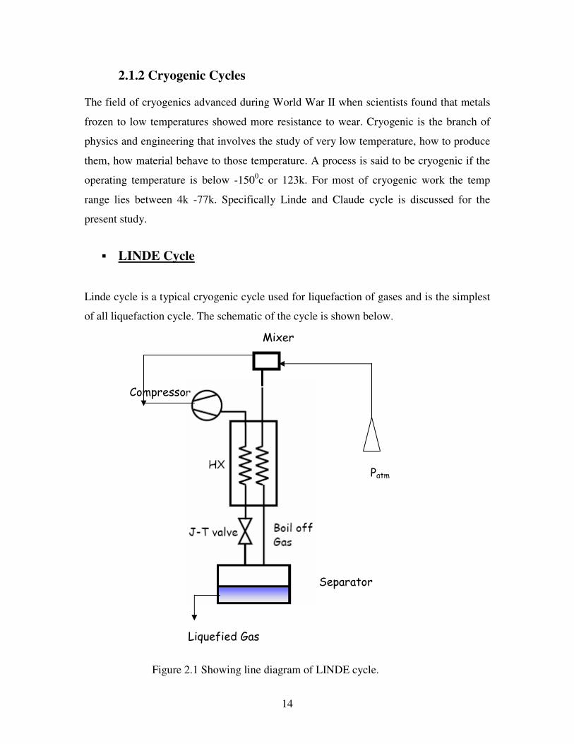
� LINDE Cycle
Linde cycle is a typical cryogenic cycle used for liquefaction of gases and is the simplest
of all liquefaction cycle. The schematic of the cycle is shown below.
Mixer
Compresso Liquefied Gas.
Patm
Separator
Liquefied Gas
Figure 2.1 Showing line diagram of LINDE cycle.

15
Figure 2.2 Showing T~S diagram of LINDE cycle.
Components Used
1. COMPRESSOR: - It is a device used to reduce the volume of gaseous air and
increase the pressure. Generally for cryogenic application compressor with high
compression ratio are used. To achieve high stage compression ratio a number of
compressor are used in series rather using a single compressor. It also reduces
work consumption. For present work isothermal compression process is used.
2. HEAT EXCHANGER: - Heat exchangers are devices which transfer heat from
hot fluid stream to cold fluid stream. In heat exchanger hot fluid temperature
decreases and there is increase in temperature of cold fluid. By losing heat hot
fluid is prepared for throttling process and similarly by gaining heat cold fluid
heated up for compression process.
3. VALVE: - A throttling valve is used to reduce the pressure of the compressed air
so that liquid air can be produced and stored. The process is assumed to be
isenthalpic expansion.

16
4. SEPARATOR/DISTILLATION COLUMN: - In this chamber air is separated
into desired components like liquid N2, liquid O2 etc and the gaseous part is again
recirculated.
5. MIXER: - It is a device helps to maintain a constant flow rate of air into the
compressor. The extra amount of air is added into incoming stream from
separator. The process is assumed to be isobaric.
A basic differentiation between the various refrigeration cycles lies in the expansion
device. This may be either an expansion engine like expansion turbine or reciprocating
expansion engine or a throttling valve. The expansion engine approaches an isentropic
process and the valve an isenthalpic process. Isentropic expansion implies an adiabatic
reversible process while isenthalpic expansions are irreversible. In the Linde’s system,
the basic principle of isenthalpic expansion is also incorporated where as in Claude’s
cycle involves both isentropic and isenthalpic expansion procedure.
� CLAUDE Cycle
The expansion through an expansion valve is an irreversible process thermodynamically
speaking. Thus if we wish to approach closer to the ideal performance, we must seek a
better process to produce lower temperatures. In the Claude system energy is removed
from the gas stream by allowing it to do some work in an expansion engine or an
expander. If the expansion engine is reversible and adiabatic, the expansion process is
isentropic and a much lower temperature is attained than that for an isenthalpic
expansion.

17
Fig 2.3 Showing a schematic of Claude Cycle with T~S diagram.
The Claude nitrogen liquefaction system differs from the simple Linde’s system by the
addition of an expander and a second heat exchanger. In this system, the nitrogen is
compressed isothermally to approximately 40 atmospheric pressure between points 1 and
2 as in figure 2.3. The high pressure nitrogen is partially cooled by passing through the
first heat exchanger between points 2 and 3.
A portion of nitrogen about 80 percent at point 3 is bled and cooled by expansion in an
expander between points 3 and 8.The remaining portion passes through the second heat
exchanger between points 3 and 4.The nitrogen from the second heat exchanger is
throttled irreversibly between points 4 and 5 at atmospheric pressure. The liquid nitrogen
is removed by the separator at point 6. The lower temperature nitrogen from the expander
at point 8 is mixed with the unliquefied nitrogen from the separator at point 7, giving the
increased mass flow of nitrogen at point 4. This nitrogen passes through the two heat
exchangers to the compressors.

18
2.2 Applications of Cryogenics
1. Cryogenic Technology is used for production of Gases for industrial and
commercial applications. In this process liquefaction and purification of Helium,
Nitrogen gases are done. Also using this technique production of inert gases is
done.
2. Cryogenics is very crucial for aerospace application. This technology is very
critical for wind tunnel testing application. High performance wind tunnel
required rapid movement of Nitrogen gas around the aerodynamic circuit.
3. Cryogenic is required for Frozen Food Industries for preservation of food item
depending upon type of food item and whether they are cooked or not before
freezing..
4. Cryogenic has got lot of application in medical field. It is wildly used in MRI
equipment for diagnosis of diseases.
5. Cryogenic has got a great role in chilled water storage system.
In particular air separation process is discussed.
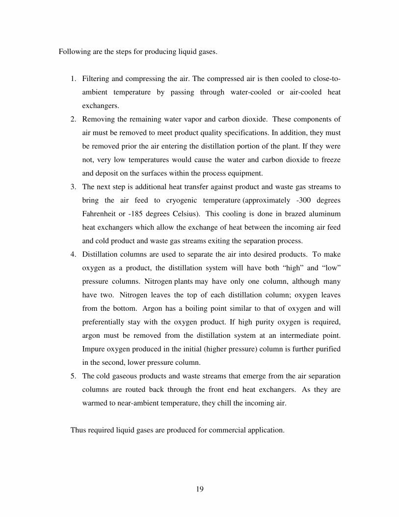
2.2.1 Air Separation Process
Cryogenic air separation process is one of the most popular air separation process used to
produce purified components of air, in particular oxygen, nitrogen, and argon. In
cryogenic gas processing various equipments like distillation column, heat exchanger,
cold inter connecting pipes are used at very low temperature. Hence all these equipments
must be well insulated. Process cycles are somewhat different depending upon how
many products are desired (either nitrogen or oxygen; oxygen and nitrogen; or nitrogen,
oxygen and argon); the required product purities; gaseous product delivery pressures; and
whether one or more products will be produced and stored in liquid form.
19
Following are the steps for producing liquid gases.
1. Filtering and compressing the air. The compressed air is then cooled to close-to-
ambient temperature by passing through water-cooled or air-cooled heat
exchangers.
2. Removing the remaining water vapor and carbon dioxide. These components of
air must be removed to meet product quality specifications. In addition, they must
be removed prior the air entering the distillation portion of the plant. If they were
not, very low temperatures would cause the water and carbon dioxide to freeze
and deposit on the surfaces within the process equipment.
3. The next step is additional heat transfer against product and waste gas streams to
bring the air feed to cryogenic temperature (approximately -300 degrees
Fahrenheit or -185 degrees Celsius). This cooling is done in brazed aluminum
heat exchangers which allow the exchange of heat between the incoming air feed
and cold product and waste gas streams exiting the separation process.
4. Distillation columns are used to separate the air into desired products. To make
oxygen as a product, the distillation system will have both “high” and “low”
pressure columns. Nitrogen plants may have only one column, although many
have two. Nitrogen leaves the top of each distillation column; oxygen leaves
from the bottom. Argon has a boiling point similar to that of oxygen and will
preferentially stay with the oxygen product. If high purity oxygen is required,
argon must be removed from the distillation system at an intermediate point.
Impure oxygen produced in the initial (higher pressure) column is further purified
in the second, lower pressure column.
5. The cold gaseous products and waste streams that emerge from the air separation
columns are routed back through the front end heat exchangers. As they are
warmed to near-ambient temperature, they chill the incoming air.
Thus required liquid gases are produced for commercial application.
20
Figure 2.4 Process Flow diagram for air distillation process.

21
CHAPTERCHAPTERCHAPTERCHAPTER----3333
22
NUMERICAL ANALYSIS
3.1 System Simulation
System simulation is the calculation of operating variables such as pressure, temperature,
and flow rates, energy of fluids in a thermal system operating in a steady state. The
equations for performance characteristics of the components and thermodynamic
properties along with energy and mass balance form a set of simultaneous equations
relating the operating variables. The mathematical description of system simulation is
that of solving these simultaneous equations many of which are non-linear.
One of the most common techniques used in simulating complex systems is the
sequential modular approach which is described subsequently.
3.2 Sequential Modular Approach
Sometimes it is possible to start with the input information and immediately calculate the
output of a component. The output information from the first component is all that is
needed to calculate the output information for the next component and so on to the final
component of the system, whose output is the output information of the system. Such a
system simulation consists of sequential calculations and hence the name sequential
modular approach.
Other methods of simulations include the Successive substitution or the Gauss Seidel
iterative technique and the Newton’s Raphsons Technique.
The various system simulation techniques were thoroughly studied and applied to
simulate some simple and complex systems which would be described subsequently.
For the present study Claude Cycle is discussed more specifically. The problem is to find
out the yield of liquid nitrogen under given conditions.

23
Figure 3.1 Flow diagram for a simple Cryogenic Cycle working on the principle of
Claude Cycle.
8
24
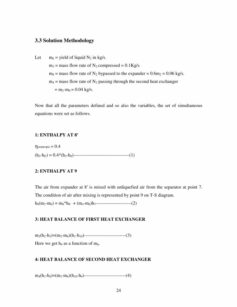
3.3 Solution Methodology
Let m6 = yield of liquid N2 in kg/s.
m2 = mass flow rate of N2 compressed = 0.1Kg/s
m8 = mass flow rate of N2 bypassed to the expander = 0.6m2 = 0.06 kg/s.
m4 = mass flow rate of N2 passing through the second heat exchanger
= m2-m8 = 0.04 kg/s.
Now that all the parameters defined and so also the variables, the set of simultaneous
equations were set as follows.
1: ENTHALPY AT 8′
ηisentropic = 0.4
(h3-h8′) = 0.4*(h3-h8)------------------------------------(1)
2: ENTHALPY AT 9
The air from expander at 8′ is mixed with unliquefied air from the separator at point 7.
The condition of air after mixing is represented by point 9 on T-S diagram.
h9(m2-m6) = m8*h8′ + (m4-m6)h7-----------------------(2)
3: HEAT BALANCE OF FIRST HEAT EXCHANGER
m2(h2-h3)=(m2-m6)(h1-h10)---------------------------(3)
Here we get h9 as a function of m6.
4: HEAT BALANCE OF SECOND HEAT EXCHANGER
m4(h3-h4)=(m2-m6)(h10-h9)---------------------------(4)
25
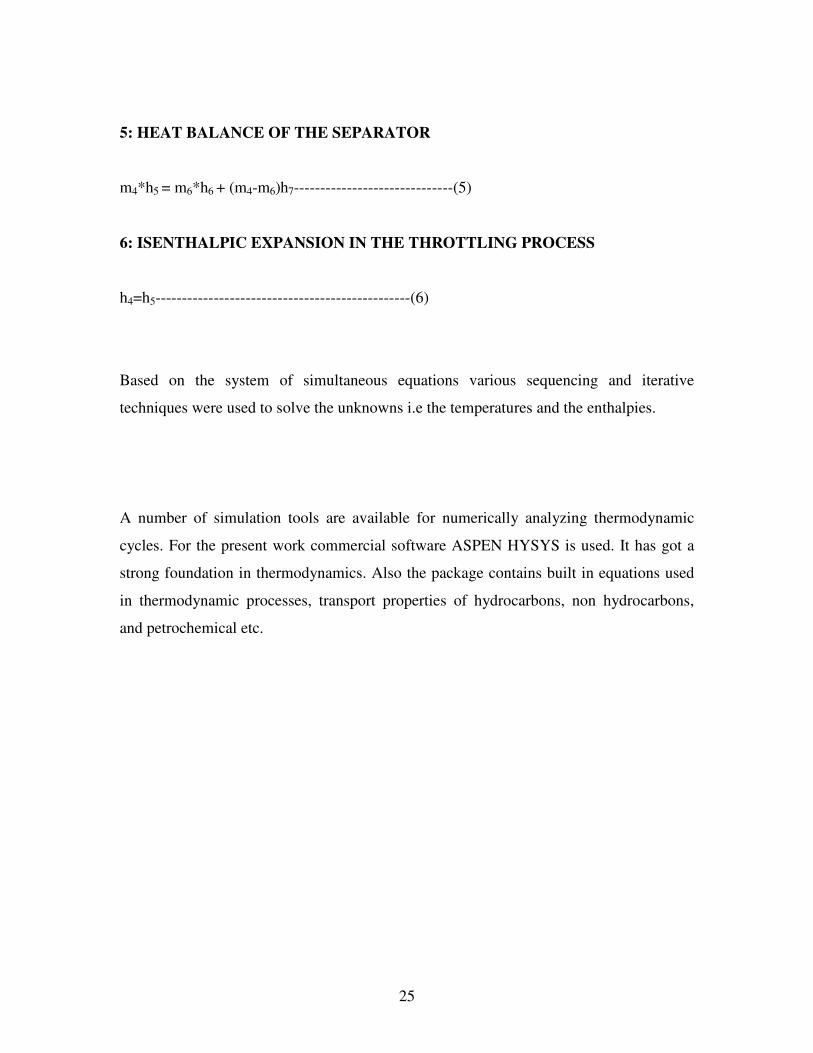
5: HEAT BALANCE OF THE SEPARATOR
m4*h5 = m6*h6 + (m4-m6)h7------------------------------(5)
6: ISENTHALPIC EXPANSION IN THE THROTTLING PROCESS
h4=h5------------------------------------------------(6)
Based on the system of simultaneous equations various sequencing and iterative
techniques were used to solve the unknowns i.e the temperatures and the enthalpies.
A number of simulation tools are available for numerically analyzing thermodynamic
cycles. For the present work commercial software ASPEN HYSYS is used. It has got a
strong foundation in thermodynamics. Also the package contains built in equations used
in thermodynamic processes, transport properties of hydrocarbons, non hydrocarbons,
and petrochemical etc.

26
CHAPTERCHAPTERCHAPTERCHAPTER----4444
27
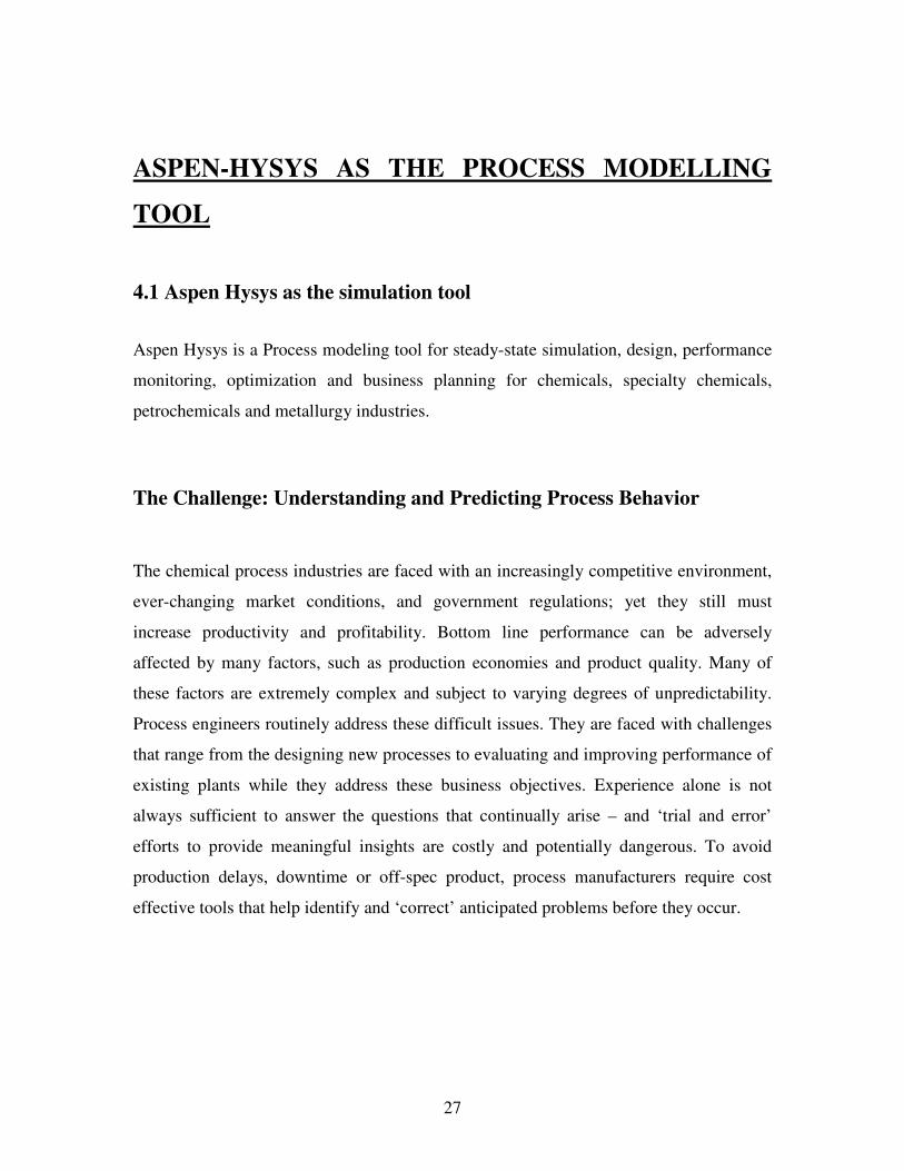
ASPEN-HYSYS AS THE PROCESS MODELLING
TOOL
4.1 Aspen Hysys as the simulation tool
Aspen Hysys is a Process modeling tool for steady-state simulation, design, performance
monitoring, optimization and business planning for chemicals, specialty chemicals,
petrochemicals and metallurgy industries.
The Challenge: Understanding and Predicting Process Behavior
The chemical process industries are faced with an increasingly competitive environment,
ever-changing market conditions, and government regulations; yet they still must
increase productivity and profitability. Bottom line performance can be adversely
affected by many factors, such as production economies and product quality. Many of
these factors are extremely complex and subject to varying degrees of unpredictability.
Process engineers routinely address these difficult issues. They are faced with challenges
that range from the designing new processes to evaluating and improving performance of
existing plants while they address these business objectives. Experience alone is not
always sufficient to answer the questions that continually arise – and ‘trial and error’
efforts to provide meaningful insights are costly and potentially dangerous. To avoid
production delays, downtime or off-spec product, process manufacturers require cost
effective tools that help identify and ‘correct’ anticipated problems before they occur.
28
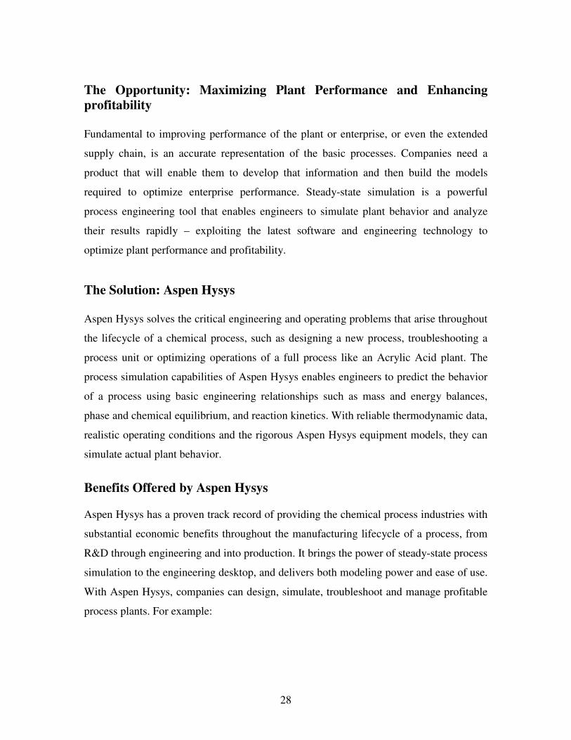
The Opportunity: Maximizing Plant Performance and Enhancing
profitability
Fundamental to improving performance of the plant or enterprise, or even the extended
supply chain, is an accurate representation of the basic processes. Companies need a
product that will enable them to develop that information and then build the models
required to optimize enterprise performance. Steady-state simulation is a powerful
process engineering tool that enables engineers to simulate plant behavior and analyze
their results rapidly – exploiting the latest software and engineering technology to
optimize plant performance and profitability.
The Solution: Aspen Hysys
Aspen Hysys solves the critical engineering and operating problems that arise throughout
the lifecycle of a chemical process, such as designing a new process, troubleshooting a
process unit or optimizing operations of a full process like an Acrylic Acid plant. The
process simulation capabilities of Aspen Hysys enables engineers to predict the behavior
of a process using basic engineering relationships such as mass and energy balances,
phase and chemical equilibrium, and reaction kinetics. With reliable thermodynamic data,
realistic operating conditions and the rigorous Aspen Hysys equipment models, they can
simulate actual plant behavior.
Benefits Offered by Aspen Hysys
Aspen Hysys has a proven track record of providing the chemical process industries with
substantial economic benefits throughout the manufacturing lifecycle of a process, from
R&D through engineering and into production. It brings the power of steady-state process
simulation to the engineering desktop, and delivers both modeling power and ease of use.
With Aspen Hysys, companies can design, simulate, troubleshoot and manage profitable
process plants. For example:
29
• The R&D group has come up with a new process for manufacturing a commodity
chemical. They have detailed physical and thermodynamic property data and have
had successful pilot plant operations. How do you evaluate the commercial
feasibility of using this process?
• The main process line has recently come up after a turnaround during which
several de-bottlenecking operations were performed. However, the results are
falling short of design. How do you explore the impact of key operating variables
upon operation of the process line to see what can be done to improve
performance?
Aspen Hysys Features
Aspen Hysys is a component of the Aspen Engineering Suite™ (AES), an integrated set
of products designed specifically to promote best engineering practices and to optimize
and automate the entire innovation and engineering workflow process throughout your
plant and across your enterprise. Automatically integrate process models with your
engineering knowledge databases, investment analyses, production optimization and
numerous other business processes. Aspen Hysys contains data, physical properties, unit
operation models, built-in defaults, reports and other features and capabilities developed
for specific industrial applications, such as electrolyte simulation. Key Aspen Hysys
features are listed below:
• Windows® Interoperability. Interface contains a process flowsheet view for
graphical layout, data browser view for entering data, the patented Next expert
guidance system to guide the user through a complete and consistent definition of
the process flowsheet.
• Plot Wizard. Enables the user to easily create plots of simulation results.
• Flowsheet Hierarchy and Templates. Collaborative engineering is supported
through hierarchy blocks that allow sub-flowsheets of greater detail to be
encapsulated in a single high-level block. These hierarchy blocks can be saved as
flowsheet templates in libraries.

30
• Equation-Oriented Modeling. Advanced specification management for equation
oriented model configuration and sensitivity analysis of the whole simulation or
specific parts of it. The unique combination of Sequential Modular and Equation
Oriented solution technology allows the user to simulate highly nested processes
encountered typically in the chemical industry.
• Thermo physical Properties. Physical property models and data are key to
generating accurate simulation results that can be used with confidence. Aspen
Hysys uses the extensive and proven physical property models, data and
estimation methods available in Aspen Properties™, which covers a wide range
of processes from simple ideal behavior to strongly non-ideal mixtures and
electrolytes. The built-in database contains parameters for more than 8,500
components, covering organic, inorganic, aqueous, and salt species and more than
37,000 sets of binary interaction parameters for 4,000 binary mixtures.
• Convergence Analysis to automatically analyze and suggest optimal tear streams,
flowsheet convergence method and solution sequence for even the largest
flowsheets with multiple stream and information recycles.
• Sensitivity Analysis to conveniently generate tables and plots showing how
process performance varies with changes to selected equipment specifications and
operating conditions.
• Design Specification capabilities to automatically calculate operating conditions
or equipment parameters to meet specified performance targets.
• Data-Fit to fit process model to actual plant data and ensure an accurate,
validated representation of the actual plant.
• Determine Plant Operating Conditions that will maximize any objective
function specified, including process yields, energy usage, stream purities and
process economics.
• Simulation Basic Manager. This feature available in Aspen Hysys for using
different fluids like nitrogen, air, acetylene as per requirement. Also several fluid
packages like BWRS, MWRS, and ASME are provided to calculate properties at
different states.

31
CHAPTERCHAPTERCHAPTERCHAPTER----5555

32
ASPEN HYSYS SIMULATIONS
For the present study an attempt has made to simulate LINDE Cycle for liquefaction of
Air and CLAUDE Cycle for liquefaction of Nitrogen. The details of two cycles are
discussed below.
5.1 Problem Specifications
5.1.1 Problem no 1.
To represent LINDE cycle as shown in figure 2.1 using ASPEN HYSYS for the
following given condition and calculate amount of liquid air is separated in the separator.
1) Mass flow rate of air 1 kg/hr at 1 bar pressure.
2) Compression Ratio 250:1.
3) Inlet temperature of air 270C
4) After throttling valve pressure drops to 1.2 bars.
5) Iso Thermal compression process in compressor.
6) Iso Enthalpic throttling in Valve.
5.1.2 Process Flow Diagram
To represent above LINDE cycle in Aspen Hysys the first step is to make a process flow
diagram (PFD). In Simulation Basic Manager a fluid package is to be selected along with
the fluid which is to be cycled in the process. For the present work air is selected as fluid
and BWRS as fluid package. Now using an option “Enter to simulation Environment”
PFD screen is started. An object palette will appear at right hand side of the screen.

33
In the object palette a number of components available some are given below.
i. Streams (Material/Energy streams)
ii. Vessels (Separator and Tanks)
iii. Heat Transfer Equipments (Heat exchanger, Valves)
iv. Rotating Equipments.
v. Piping Equipments.
vi. Solid Handling.
vii. Reactor.
viii. Logical.
ix. Sub Flow sheet.
x. Short Cut Column.
Streams
Compressors
Mixer
Object Palette.
Recycler

34
Some of the components used.
Where P-100 is a centrifugal pump.
K-100 is a compressor.
K-101 is an expander.
Where MIX-100 is a mixer.
VLV-100 is a valve.
LNG-100 is a LNG heat exchanger.
V-100 3-phase separator.
35
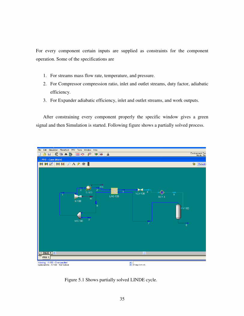
For every component certain inputs are supplied as constraints for the component
operation. Some of the specifications are
1. For streams mass flow rate, temperature, and pressure.
2. For Compressor compression ratio, inlet and outlet streams, duty factor, adiabatic
efficiency.
3. For Expander adiabatic efficiency, inlet and outlet streams, and work outputs.
After constraining every component properly the specific window gives a green
signal and then Simulation is started. Following figure shows a partially solved process.
Figure 5.1 Shows partially solved LINDE cycle.

36
Above process is partially solved because all the streams are not in blue color (4, 5
streams). Following figure shows a solved LINDE cycle with all streams in blue.
Figure 5.2 Flowsheet for LINDE cycle created in Aspen Hysys.
5.1.3 Basic description of the flowsheet
The above flowsheet in Aspen Hysys shows the various components and the material
streams needed to bring about the liquefaction of the air. It consists of a mixer, an
isentropic compressor, a cooler, a shell and tube countercurrent heat exchanger, an
isenthalpic J-T valve, a separator which performs flash operations and a splitter which
takes care of the mass convergence problems. These components or the equipments are
termed as the blocks in the language of Aspen Hysys.
37
5.1.4 The Process
A Fresh feed stream of air at 300K and 1.0 bar enters the mixer, goes through the
compressor where both pressure and temperature both increases. The temperature of the
output feed stream is usually in the order of >400 K and hence it has to be cooled before
entering the shell and tube heat exchanger. Hence an intermediate after cooler is used so
as to bring down the temperature of the hot fluid in the order of around 300 K. The hot
fluid enters the tube side inlet whereby it is cooled down by the downstream shell side
cold stream. Then it goes through an isenthalpic J-T valve whereby an isenthalpic flash
results in decreasing the temperature of the fluid. The vapor fraction is usually of the
order of 0.92 and it can be decreased or alternatively the cold can be increased taking
care of the heat exchanger performance. The vapor liquid mixture which comes out of the
valve enters the separator where the separator flashes the vapor liquid mixture and the
desired liquid air can be collected from bottom. The remaining vapor rises and is directed
towards the shell side of the heat exchanger where by its temperature increases. The out
stream from the heat exchanger cannot be directly mixed with the feed stream as it results
in some convergence problems. This can be taken care off by using a mixer with a
specified mix fraction. This mixer purges a fraction of the recycled outlet stream from the
heat exchanger and gradually mixes the whole of the incoming recycle stream with the
fresh feed and the cycle goes on.
5.1.5 The components or the blocks or the equipments
The description of the various components and the conditions at which they operate are
described subsequently.
a: Mixer (MIX-100)
The outlet and the inlet pressure to be the same = 1.0 bar inside the mixture whose main
purpose is to mix two incoming streams and send the outlet stream at some intermediate
and equilibrium state. We consider a fresh feed stream of Air entering the mixer at 300 K
and 1.0 Bar at the rate of 1 Kg/hr and also the final recycle stream entering into it at the
38
same pressure. These two streams mix and the output stream 1 goes to the compressor.
The temperature estimate is roughly given a guess of 300 K.
b: Compressor (K-100)
The compressor is modeled to be isentropic with an isentropic efficiency of 85%. The
discharge pressure is 250 bars and hence a pressure ratio of 250/1.0 is considered.
c: After Cooler(E-100)
The pressurized stream that comes out of the compressor is too hot to enter into the tube
side of the heat exchanger and hence an after cooler with a flash specification of 300 K
temperature and 250 bars is considered. There are no pressure drops inside it.
d: Heat exchanger(LNG-100)
The heat exchanger as used in the simulation is a countercurrent shell and tube heat
exchanger where the hot fluid flows through the tube side and the cold fluid through the
shell side. A pressure drop of 1 bar is occurring during the flow in hot stream and 0.2 bar
in cold stream. The exchanger duty is given an initial guess a minimum temperature
approach of 10 K is estimated.
e: J-T Valve(VLV-100)
An isentropic J-T valve is used in LINDE cycle which works at a constant enthalpy and is
such that with decrease in pressure an appreciable drop in temperature is brought about.
The specification given is with a calculation type of Adiabatic flash for specified outlet
pressure and a pressure drop of 247.8 bars. The valid phases are vapor liquid mixture.
f: Phase separator(V-100)
For the purpose of flashing the vapor liquid mixture that comes out of the J-T valve, a
phase separator is used with the flash specifications given with pressure =1.2 bar and a
temperature of 90K which is just a guess value to start the iterative technique.
39
g: Recycler(RCY-1)
It is used for checking the convergence criteria. Generally at the place of under-constraint
situation this is used to restrict the degree of freedom. After the convergence input and
output conditions are with in the tolerance limit.
The inputs for the various blocks were given systematically including the guess values so
that all the minimum informations were available and the simulation was ready to run.
The following data are available with us,
1: Temperature of feed=300 K
2: LP=1.0 bar in the LINDE cycle
3: HP=250 bar in the LINDE cycle
4: Mass flow rate of the feed stream=1 Kg/hr
5: Isentropic efficiency of the compressor=85%
Simulation results for the above LINDE cycle will be discussed in chapter-6. To
increases the amount of liquefaction rate and efficiency of process some modification are
made and an extra turbo expander is used along with a more Heat Exchanger. Detail
specifications for CLAUDE cycle is mentioned as Problem no 2.

40
5.2.1 Problem no 2.
To represent CLAUDE cycle as shown in figure 2.3 using ASPEN HYSYS for the
following given condition and calculate amount of liquid N2 is separated and the
optimum condition for maximum liquid output.
1. Operating Pressure (inlet) = 1 bar.
2. Compression Ratio 40:1.
3. Isothermal compression in compressor.
4. Inlet temperature N2 of 270C.
5. After throttling valve pressure drops to 1.3 bars.
6. Iso Enthalpic throttling in Valve.
7. Expander Efficiency varies from 0.4 to 0.6.
8. Fraction of liquid separated from main stream varies 0.6 to 0.8.
9. Volume flow rate of liquid N2 is 300 nm3/hr.
Where 300 nm3/hr. can be converted to mass flow rate. It is found to be 0.11 Kg/s
at a temp 300K. (From simple Gaseous principles).
5.2.2 Process Flow Diagram
To represent above CLAUDE cycle in Aspen Hysys the first step is to make a process
flow diagram (PFD). In Simulation Basic Manager a fluid package is to be selected along
with the fluid which is to be cycled in the process. For the present work N2 is selected as
fluid and BWRS as fluid package. Now using an option “Enter to simulation
Environment” PFD screen is started. An object palette will appear at right hand side of
the screen. Components like compressor, LNG heat exchangers, J-T Valve, 3-Phase
Separator, Turbo expander, Mixer, Recyclers are selected to draw PFD. These
components or the equipments are termed as the blocks in the language of Aspen Hysys.
Following figure 5.3 shows flowsheet diagram of CLAUDE cycle.
41
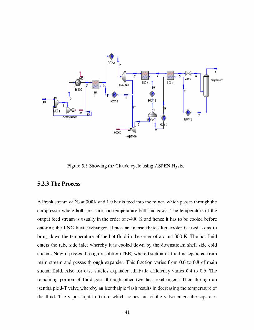
Figure 5.3 Showing the Claude cycle using ASPEN Hysis.
5.2.3 The Process
A Fresh stream of N2 at 300K and 1.0 bar is feed into the mixer, which passes through the
compressor where both pressure and temperature both increases. The temperature of the
output feed stream is usually in the order of >400 K and hence it has to be cooled before
entering the LNG heat exchanger. Hence an intermediate after cooler is used so as to
bring down the temperature of the hot fluid in the order of around 300 K. The hot fluid
enters the tube side inlet whereby it is cooled down by the downstream shell side cold
stream. Now it passes through a splitter (TEE) where fraction of fluid is separated from
main stream and passes through expander. This fraction varies from 0.6 to 0.8 of main
stream fluid. Also for case studies expander adiabatic efficiency varies 0.4 to 0.6. The
remaining portion of fluid goes through other two heat exchangers. Then through an
isenthalpic J-T valve whereby an isenthalpic flash results in decreasing the temperature of
the fluid. The vapor liquid mixture which comes out of the valve enters the separator

42
where the separator flashes the vapor liquid mixture and the desired liquid N2 can be
collected from bottom. The remaining vapor rises and is directed towards the shell side of
the heat exchanger where by its temperature increases. The out stream from the heat
exchanger (HX-3) get mixed with the expanded stream coming from expander and passes
through the other two heat exchangers. The out stream from the heat exchanger cannot be
directly mixed with the feed stream as it results in some convergence problems. This can
be taken care off by using a mixer with a specified mix fraction. This mixer purges a
fraction of the recycled outlet stream from the heat exchanger and gradually mixes the
whole of the incoming recycle stream with the fresh feed and the cycle goes on.
5.2.4 The components or the blocks or the equipments
The description of the various components and the conditions at which they operate are
described subsequently.
a: Mixer (MIX-1, MIX-2)
The outlet and the inlet pressure to be the same = 1.0 bar inside the mixture (MIX-1)
whose main purpose is to mix two incoming streams and send the outlet stream at some
intermediate and equilibrium state. A fresh feed stream of N2 entering the mixer at 300 K
and 1.0 Bar at the rate of 0.1 Kg/s and also the final recycle stream entering into it at the
same pressure. These two streams mix and the output stream 1 goes to the compressor.
The temperature estimate is roughly given a guess of 300 K. In the other mixture (MIX-
2) the streams coming from expander and third heat exchanger mixes.
b: Compressor
The compressor is modeled to be isentropic with an isentropic efficiency of 85%. The
discharge pressure is 40 bars and hence a pressure ratio of 40/1.0 is considered.
43
c: After Cooler(E-100)
The pressurized stream that comes out of the compressor is too hot to enter into the tube
side of the heat exchanger and hence an after cooler with a flash specification of 300 K
temperature and 40 bars is considered. There are no pressure drops inside it.
d: Heat exchanger(HX-1, HX-2, HX-3)
The heat exchanger as used in the simulation is a countercurrent shell and tube heat
exchanger where the hot fluid flows through the tube side and the cold fluid through the
shell side. A pressure drop of 0.1 bars occurring during the flow in each stream. The
exchanger duty is given an initial guess a minimum temperature approach of 10 K is
estimated.
e: Splitter(TEE-100)
Stream 3 coming from HX-1 is passed through splitter which separates a definite fraction
of (0.6 to 0.8) fluid from main stream and allowed to bled later stage. The remaining
portion of the fluid moves through other heat exchangers. This separation helps to
achieve lower temperature and desired output conditions.
f: J-T Valve
An isentropic J-T valve is used in CLAUDE cycle which works at a constant enthalpy
and is such that with decrease in pressure an appreciable drop in temperature is brought
about. The specification given is with a calculation type of Adiabatic flash for specified
outlet pressure and a pressure drop of 38.4 bars. The valid phases are vapor liquid
mixture.
g: Phase separator
For the purpose of flashing the vapor liquid mixture that comes out of the J-T valve, a
phase separator is used with the flash specifications given with pressure =1.3 bar and a
temperature of 90K which is just a guess value to start the iterative technique.
44
h: Expander
It a rotating device used for expansion of separated fluid in the splitter. The expansion
process is assumed to be isentropic. Adiabatic efficiency of expander is varied from 0.4
to 0.6 for different case studies.
i: Recycler(RCY-1, RCY-2, RCY-3, RCY-4, RCY-5)
It is used for checking the convergence criteria. Generally at the place of under-constraint
situation this is used to restrict the degree of freedom. After the convergence input and
output conditions are with in the tolerance limit.
The inputs for the various blocks were given systematically including the guess values so
that all the minimum information was available and the simulation was ready to run.
The following data are available with us,
1: Temperature of feed=300 K
2: LP=1.0 bar in the CLAUDE cycle
3: HP=250 bar in the CLAUDE cycle
4: Mass flow rate of the feed stream=0.1 Kg/s
5: Isentropic efficiency of the compressor=85%
6: Expander efficiency = 0.4, 0.5, 0.6.
7: Fraction of fluid separated = 0.6, 0.62, 0.64, 0.66…etc.
Simulation results for the above CLAUDE cycle will be discussed in chapter-6. Also a
comparison between LINDE and CLAUDE cycle is done to show the more efficient
process of liquefaction.

45
CHAPTERCHAPTERCHAPTERCHAPTER----6666

46
RESULTS AND DISCUSSIONS
In this chapter simulation results for both LINDE and CLAUDE are discussed separately
and later a comparison is made between those to verify which cycle is better for
liquefaction process.
6.1 LINDE Cycle Simulation Results.
Figure 6.1 showing the PFD of LINDE Cycle
As previously discussed the objective is to find out amount of liquid air output (stream 6).
The details of mass flow rate, temperature, vapor fraction, pressure are given in tabulated
format below.
47
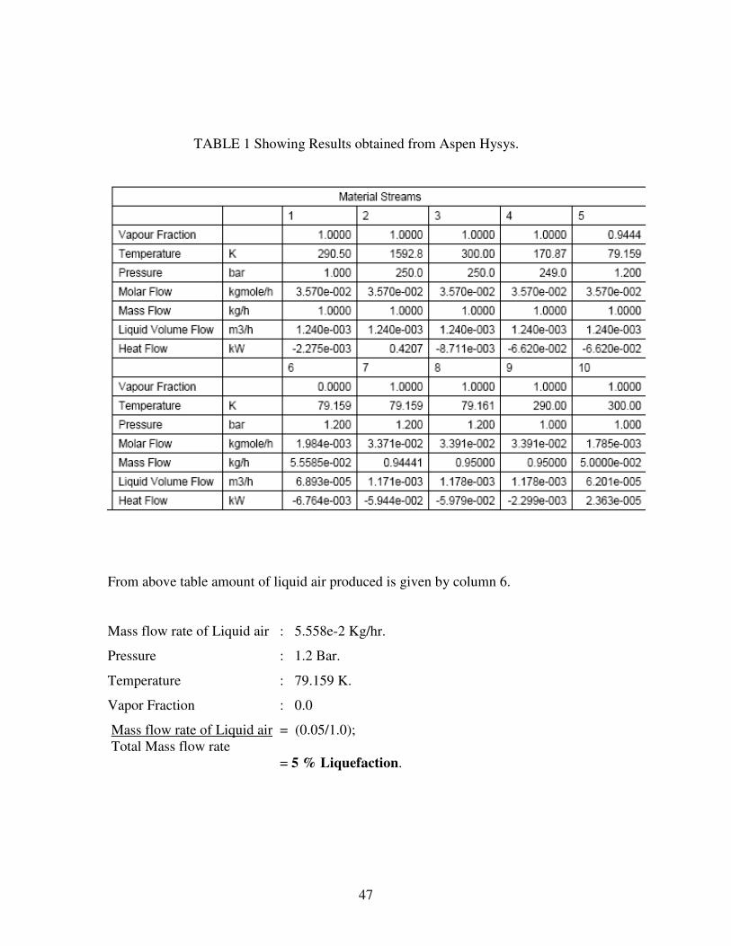
TABLE 1 Showing Results obtained from Aspen Hysys.
From above table amount of liquid air produced is given by column 6.
Mass flow rate of Liquid air : 5.558e-2 Kg/hr.
Pressure : 1.2 Bar.
Temperature : 79.159 K.
Vapor Fraction : 0.0
Mass flow rate of Liquid air = (0.05/1.0);
Total Mass flow rate
= 5 % Liquefaction.
48
6.1.1 GRAPHS:-
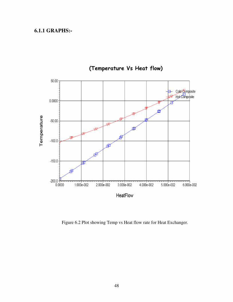
(Temperature Vs Heat flow)
Figure 6.2 Plot showing Temp vs Heat flow rate for Heat Exchanger.
49
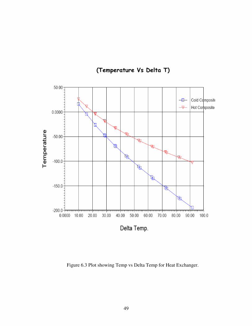
(Temperature Vs Delta T)
Figure 6.3 Plot showing Temp vs Delta Temp for Heat Exchanger.
50
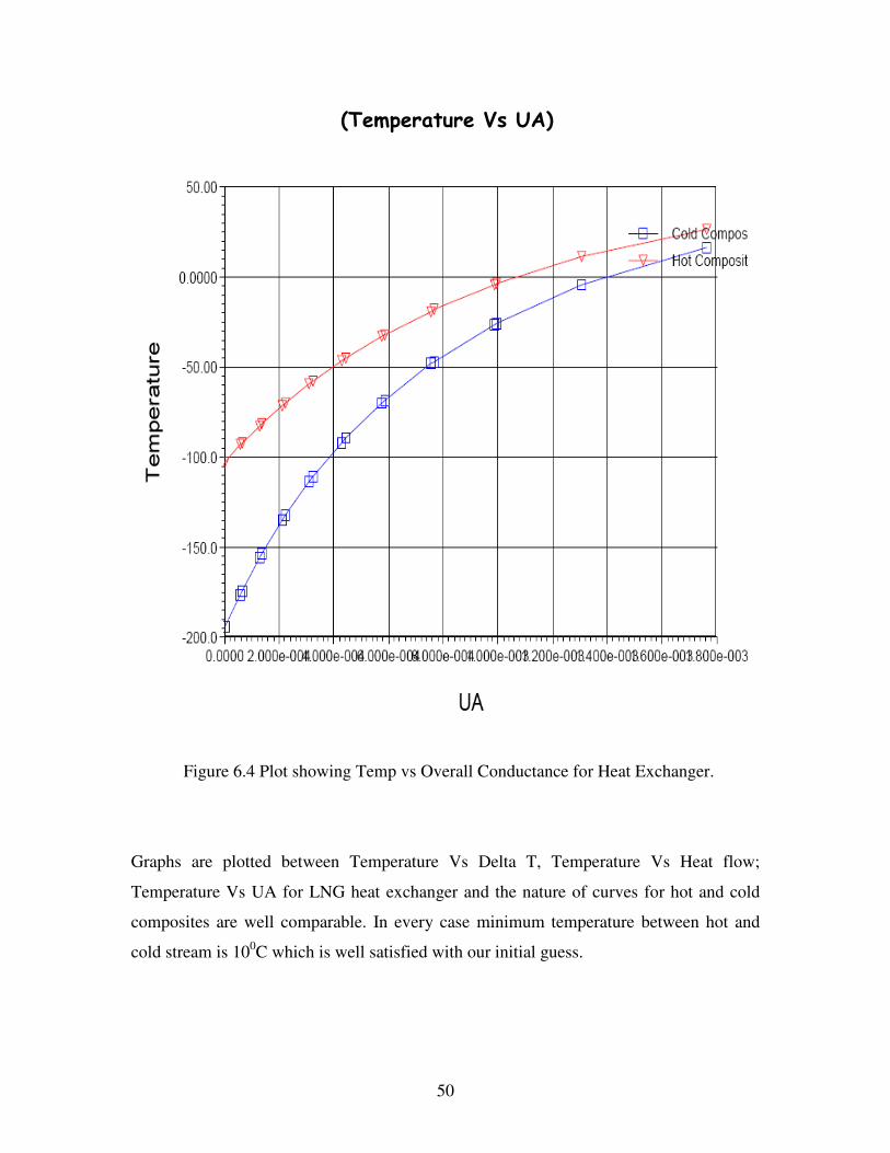
(Temperature Vs UA)
Figure 6.4 Plot showing Temp vs Overall Conductance for Heat Exchanger.
Graphs are plotted between Temperature Vs Delta T, Temperature Vs Heat flow;
Temperature Vs UA for LNG heat exchanger and the nature of curves for hot and cold
composites are well comparable. In every case minimum temperature between hot and
cold stream is 100C which is well satisfied with our initial guess.
51
6.2 CLAUDE Cycle Simulation Results.
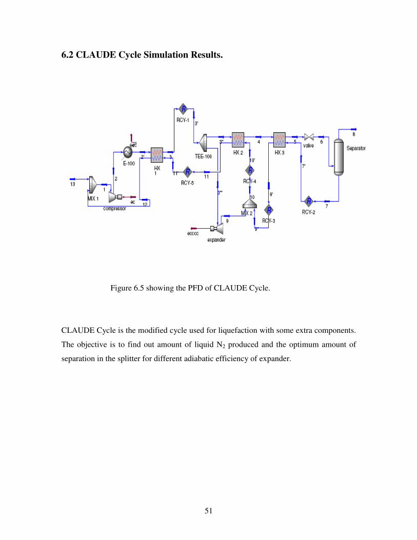
Figure 6.5 showing the PFD of CLAUDE Cycle.
CLAUDE Cycle is the modified cycle used for liquefaction with some extra components.
The objective is to find out amount of liquid N2 produced and the optimum amount of
separation in the splitter for different adiabatic efficiency of expander.

52
Attach the pics…………newclaude2.pdf
53
Above table shows the optimum flow rate condition for expander efficiency 40% and
separation through splitter is 0.68 of the main stream fluid. The column 7 shows the
amount of liquid N2 produced.
Mass flow rate of liquid N2 : 8.635e-003 kg/s.
Temperature : 79.55 K
Vapor fraction : 0.0
Pressure : 1.3 bars.
Mass flow rate of liquid N2 = (0.00864/ 0.032)
(Total Mass flow rate of liquid N2
in main stream after separation)
= 27 % of liquefaction.
Now the graphs are plotted to know the temperature variation of three Heat Exchangers
used. Those are shown below.

54
6.2.1 GRAPHS
(((( For HXFor HXFor HXFor HX----1111 ))))
Figure 6.6 Plot showing Temp vs HeatFlow for Heat Exchanger -1.
55
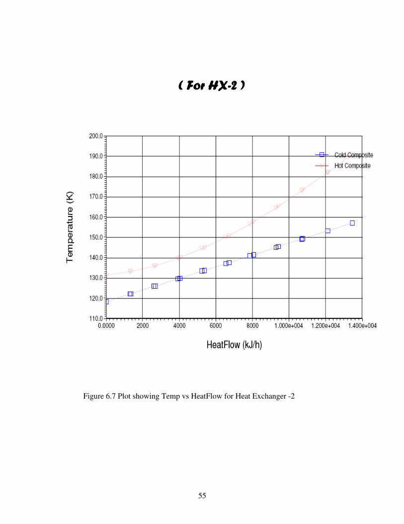
(((( For For For For HXHXHXHX----2 2 2 2 ))))
Figure 6.7 Plot showing Temp vs HeatFlow for Heat Exchanger -2

56
(((( For For For For HXHXHXHX----3 3 3 3 ))))
Figure 6.8 Plot showing Temp vs HeatFlow for Heat Exchanger -3.
Above graphs show that in all heat exchanger minimum approach is 10K. Also the
variation of temperature is well comparable with the theoretical results. It should be noted
that in HX-3 the hot stream temp reduction is very less (<10K). This gives a idea for the
future work for completing the CLAUDE cycle with out HX-3.

57
As mentioned earlier a number of simulations are done by varying the efficiency of turbo
expander. Those are discussed as different Cases in following. The objective of present
work is to find out optimum condition for maximum liquefaction.
Case1: ( Expander adiabatic efficiency 40% )
Fraction of flow in main
stream(3’’) after separation in
splitter.
Liquid N2 in Kg/s.
0.28 8.21E-03
0.3 8.35E-03
0.32 8.64E-03
0.34 8.58E-03
0.36 8.27E-03
0.38 8.21E-03
0.4 7.96E-03
0.42 7.96E-03
0.44 7.82E-03
0.46 7.63E-03
From above table the mass flow rate is found maximum for the fraction of separation
0.32. An excel plot is made using above data to show the peak value.
58
For 40% Expander efficiency
6.80E-037.00E-037.20E-037.40E-037.60E-037.80E-038.00E-038.20E-038.40E-038.60E-038.80E-03
0.28
0.32
0.36 0.
40.
440.
48
Fraction of N2 passing through main
stream
Liq
uid
N2
in
Kg
/s.
Series1
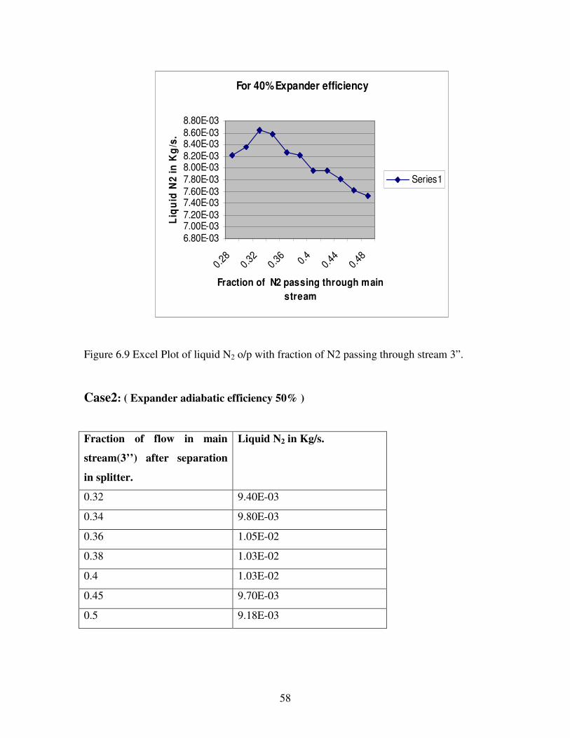
Figure 6.9 Excel Plot of liquid N2 o/p with fraction of N2 passing through stream 3”.
Case2: ( Expander adiabatic efficiency 50% )
Fraction of flow in main
stream(3’’) after separation
in splitter.
Liquid N2 in Kg/s.
0.32 9.40E-03
0.34 9.80E-03
0.36 1.05E-02
0.38 1.03E-02
0.4 1.03E-02
0.45 9.70E-03
0.5 9.18E-03

59
For 50% Expander efficiency
8.50E-03
9.00E-03
9.50E-03
1.00E-02
1.05E-02
1.10E-02
0.32
0.34
0.36
0.38 0.
40.
45 0.5
Fraction of N2 passing through
main stream
Liq
uid
N2 in
Kg
/sSeries1
Figure 6.10 Excel Plot of liquid N2 o/p with fraction of N2 passing through stream 3”.
An excel plot is made using above data which show the maximum output is at 0.36
fraction of separation.
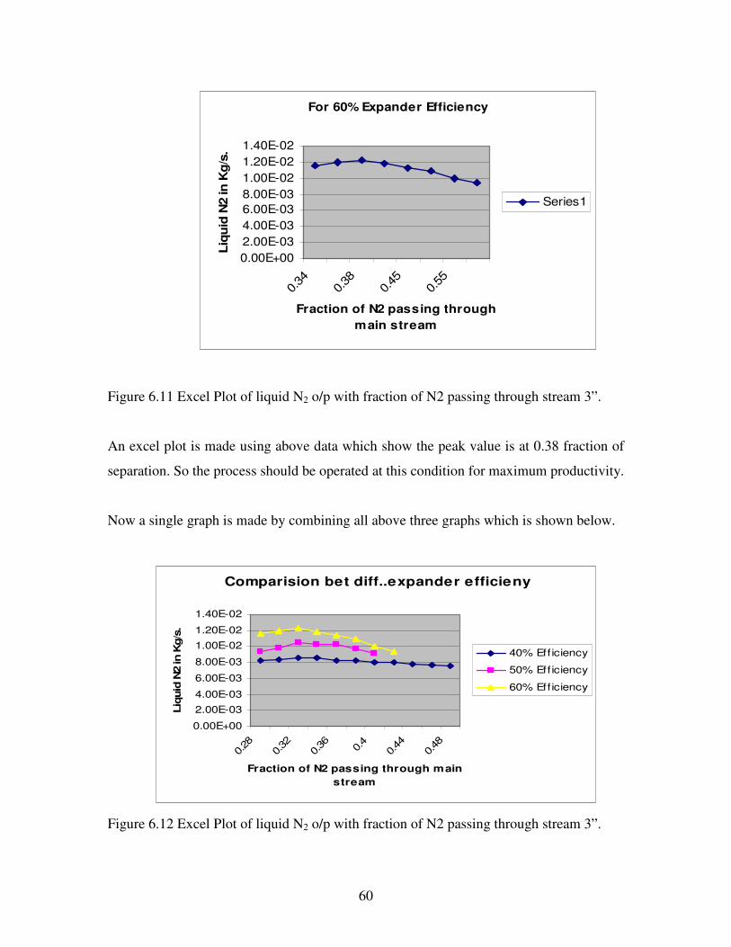
Case3: ( Expander adiabatic efficiency 60% )
Fraction of flow in main
stream(3’’) after separation
in splitter.
Liquid N2 in Kg/s.
0.34 1.16E-02
0.36 1.20E-02
0.38 1.23E-02
0.4 1.19E-02
0.45 1.14E-02
0.5 1.09E-02
0.55 1.00E-02
0.6 9.37E-03
60
For 60% Expander Efficiency
0.00E+00
2.00E-03
4.00E-03
6.00E-03
8.00E-03
1.00E-02
1.20E-02
1.40E-02
0.34
0.38
0.45
0.55
Fraction of N2 passing through
main stream
Liq
uid
N2 in
Kg
/s.
Series1
Figure 6.11 Excel Plot of liquid N2 o/p with fraction of N2 passing through stream 3”.
An excel plot is made using above data which show the peak value is at 0.38 fraction of
separation. So the process should be operated at this condition for maximum productivity.
Now a single graph is made by combining all above three graphs which is shown below.
Comparision bet diff..expander efficieny
0.00E+00
2.00E-03
4.00E-03
6.00E-03
8.00E-03
1.00E-02
1.20E-02
1.40E-02
0.28
0.32
0.36 0.
40.44
0.48
Fraction of N2 passing through main
stream
Liq
uid
N2 in K
g/s
.
40% Efficiency
50% Efficiency
60% Efficiency
Figure 6.12 Excel Plot of liquid N2 o/p with fraction of N2 passing through stream 3”.
61
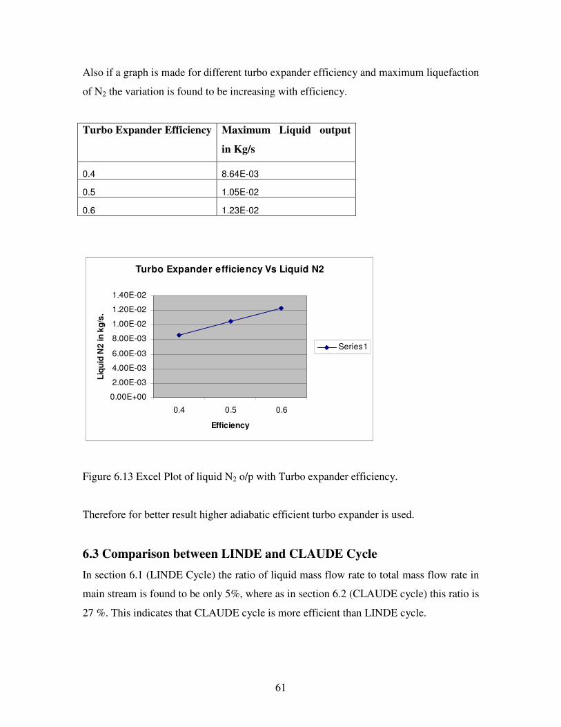
Also if a graph is made for different turbo expander efficiency and maximum liquefaction
of N2 the variation is found to be increasing with efficiency.
Turbo Expander Efficiency Maximum Liquid output
in Kg/s
0.4 8.64E-03
0.5 1.05E-02
0.6 1.23E-02
Turbo Expander efficiency Vs Liquid N2
0.00E+00
2.00E-03
4.00E-03
6.00E-03
8.00E-03
1.00E-02
1.20E-02
1.40E-02
0.4 0.5 0.6
Efficiency
Liq
uid
N2
in
kg
/s.
Series1
Figure 6.13 Excel Plot of liquid N2 o/p with Turbo expander efficiency.
Therefore for better result higher adiabatic efficient turbo expander is used.
6.3 Comparison between LINDE and CLAUDE Cycle
In section 6.1 (LINDE Cycle) the ratio of liquid mass flow rate to total mass flow rate in
main stream is found to be only 5%, where as in section 6.2 (CLAUDE cycle) this ratio is
27 %. This indicates that CLAUDE cycle is more efficient than LINDE cycle.

62
CHAPTERCHAPTERCHAPTERCHAPTER----7777

63
CONCLUSION
7.1 Summery of the Work Done
Simulation of cryogenic cycles was done using the commercial software ASPEN
HYSYS. In the present work Cryogenic cycles like LINDE cycle was used for
liquefaction of air which yields only 5 % of liquid air at the end of the process. To
increase the productivity one more modified cycle was used know as CLAUDE cycle
where the liquefaction rate increases to 27 %. Also the work was extended to study
CLAUDE with different adiabatic efficiency condition of the expander and optimum
condition for the maximum liquid output was found out. Detailed graphical
representations of various cases were also done.
7.2 Future Scope.
This project work simulates a LINDE cycle, CLAUDE Cycle using the simulation tool
ASPEN HYSYS. The results obtained from simulation will helps to carry out
experiments in lab at optimum condition and in later stages comparison can be made.
Much complex cycles like the Kaptiza cycle, Heylandt Cycle , Collins liquefaction cycle
for liquefaction of Nitrogen can also be simulated using the same ASPEN HYSYS. User
defined functions can also be incorporated to solve complex real life simulations.

64
CHAPTERCHAPTERCHAPTERCHAPTER----8888
65
BIBLIOGRAPHY
1. Barron Randall F., ‘Cryogenic Systems’, New York, Oxford University Press,
1985.
2. Flynn Thomas M., ‘Cryogenic Engineering’, Colorado, Oxford University
Press, 1992.
3. Stoecker W.F, ‘Design of Thermal systems’, Toronto, Tata McGraw Hill, 1986.
4. Aspen Tutorial #1: Aspen Basic
5. Aspen Tutorial #4: Thermodynamic Method.
6. Aspen simulation by Chuen Chan, Dept of Chemical Engineering.
7. Design Modeling and simulation of air liquefaction by John E. Crowley, School
of Aerospace Engineering Space Systems Design Lab Georgia Institute of
Technology.