nmr facility - university of washington€¦ · at the nmr facility, department of chemistry, uw....
TRANSCRIPT

NMR FACILITY DEPARTMENT OF CHEMISTRY
University of Washington
TOPSPIN 2.1
TRAINING NOTES
February 2011 rajan paranji
2
CONTENTS
3
Introduction
View of TOPSPIN INTERFACE 6
Operating the Bruker Spectrometer – WORK FLOW 7
LOGON 8
SAMPLE HANDLING 9
DATA SET DEFINITION 10
LOCKING AND SHIMMING 14
PARAMETER OPTIMIZATION 18
ACQUISITION 21
PROCESSING
FT 22
PHASE CORECTION 22
INTEGRATION 24
PEAK PICKING 28
PLOTTING 30
CLEANUP 36
APPENDIX
A DOT COMMANDS AND KEYBOARD SHORTCUTS 38
B COMMONLY USED PARAMETERS IN TOPSPIN 40
C COMMONLY USED COMMANDS IN TOPSPIN 45
3
Introduction
Topspin is a versatile and user-friendly software interface to both control the Bruker NMR
spectrometer and process the raw data. For those users who are only familiar with the older
generation Bruker software i.e. XWINNMR, the good news is that, (almost) all the commands you type
on the command line are still valid in Topspin interface. Very few commands have disappeared, due to
the evolution of both the hardware and software of the spectrometer. An example is the command ‘cfbsms’, which used to reset the BSMS interface.
But Topspin is much more than what XWINNMR was capable of doing. There are three different levels
at which you can use this software (1) Novice (2) Routine user and (3) Expert. The software is built in
a layered manner so that the same interface provides just the needed commands and operations that
is needed at the level you are operating.
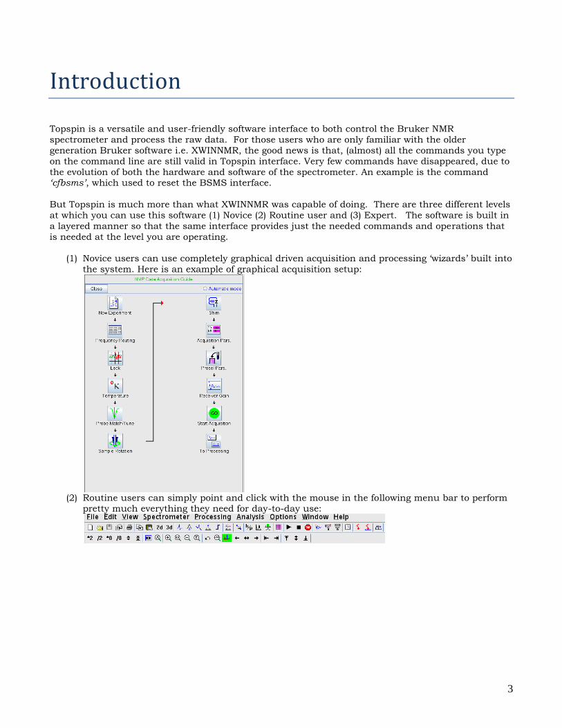
(1) Novice users can use completely graphical driven acquisition and processing ‘wizards’ built into
the system. Here is an example of graphical acquisition setup:
(2) Routine users can simply point and click with the mouse in the following menu bar to perform
pretty much everything they need for day-to-day use:

4
(3) Experts can dig deeper for powerful features that exploit spectrometer hardware to the full.
Here is an example of the shaped pulse optimization tool:
The best way is to explore freely, with a temporary dataset open.
This manual is written as a companion to the one-on-one NMR training course that is currently offered
at the NMR Facility, Department of Chemistry, UW. Decidedly, this manual only scratches the surface
of explaining the features of Topspin software. But it can be, in principle, used as a ‘Do It Yourself’ for accomplishing the rudimentary tasks of setting up a 1D proton or Carbon experiment, record data and
process it.
There are two useful features of Topspin interface, which you should exploit fully, to get instant help
about a particular feature.
(1) The Help Menu located in the top right part of the Menu panel :
(2) You can type on the command line: help <keyword>. For instance you can type help ased
and you will get the following web browser page that explains the ased command in detail:

5
Please feel free to ask for help from Facility Staff by phone, email or by paging :
Rajan K Paranji NMR Facility Manager
Room:65, Bagley Hall
Department of Chemistry
University of Washington
phone: 206 685 2581
email: [email protected]
Paul Miller Assistant Manager
Room: 57, Bagley Hall
Department of Chemistry
University of Washington
phone: 206 543 1662
email: [email protected]
pager: 206 997 6220

6
TOPSPIN MAIN INTERFACE
7
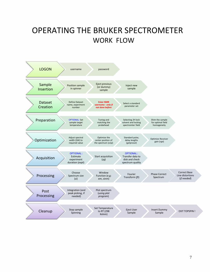
OPERATING THE BRUKER SPECTROMETER WORK FLOW
LOGON username password
Sample Insertion
Position sample in spinner
Eject previous (or dummy)
sample
Inject new sample
Dataset Creation
Define Dataset name, experiment
number
Enter NMR username - only if not done before
Select a standard parameter set
Preparation OPTIONAL: Set sample target temperature
Tuning and matching the
probehead
Selecting 2H lock solvent and locking spectromter field
Shim the sample for optimal field
homogeneity
OptimizationAdjust spectral width (SW) to required value
Optimize the center position of
the spectrum (o1p)
Standard pulse, delay lengths
(getprosol)
Optimize Receiver gain (rga)
AcquisitionOPTIONAL :
Estimate experiment
duration (expt)
Start acquisition (zg)
OPTIONAL : Transfer data to disk and check
spectrum quality
ProcessingChoose
Spectrum size (si)
Window Function (e.g:
em, sinm)
Fourier Transform (ft)
Post Processing
Phase Correct Spectrum
Correct Base Line distortions
(if needed)
Integration (and peak picking, if
needed)
Plot spectrum (using plot program)
Cleanup Stop sample Spinning
Set Temperature to RT (298
Kelvin)
Eject User Sample
Insert Dummy Sample
EXIT TOPSPIN !

8
LOGON
Username: genuser (OR) UWNetid
Password: nmr301
Instrument Name
Base Frequency
Instrument suffix
AV300 300.13 MHz 300
AV301 300.13 MHz 301
AV500 499.044 MHz 500
DRX499 499.85 MHz 499
DPX200 200.12 MHz 200
Password for any instrument is “nmr” followed by the instrument suffix in the table below.
9
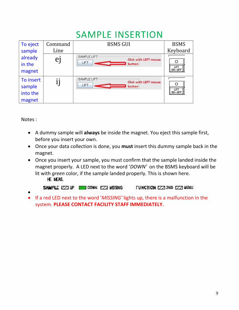
SAMPLE INSERTION To eject sample already in the magnet
Command Line
BSMS GUI BSMS Keyboard
ej
To insert sample into the magnet
ij
Notes :
A dummy sample will always be inside the magnet. You eject this sample first, before you insert your own.
Once your data collection is done, you must insert this dummy sample back in the magnet.
Once you insert your sample, you must confirm that the sample landed inside the magnet properly. A LED next to the word ‘DOWN’ on the BSMS keyboard will be lit with green color, if the sample landed properly. This is shown here.
If a red LED next to the word ‘MISSING’ lights up, there is a malfunction in the
system. PLEASE CONTACT FACILITY STAFF IMMEDIATELY.

10
DATA SET DEFINITION To define new Data Set
Command Line
TOPSPIN GUI
new or
edc
Notes :
USER is the NMR User name (in the future this will be your UWNetid and cannot
be changed)
Next to NAME, enter a meaningful name for the dataset.
Next to EXPNO, enter a numerical value (1, 2,...10,...)
Default value for PROCNO is 1 and can be left as it is
Click on
Describe your experiment or sample here. (Can be imported
later into the plot window.)
11
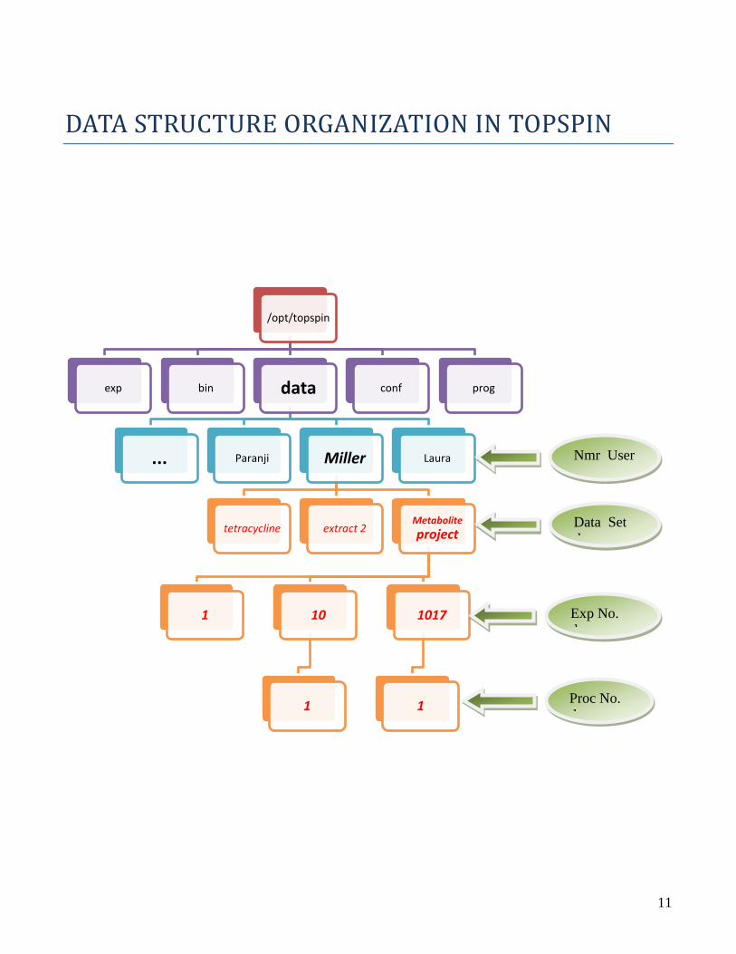
DATA STRUCTURE ORGANIZATION IN TOPSPIN
/opt/topspin
exp bin data
... Paranji Miller
tetracycline extract 2Metabolite
project
1 10
1
1017
1
Laura
conf prog
Nmr User
Data Set
d
Exp No.
d
Proc No.
d

12
Standard Parameter Sets
Following standard parameter sets are predefined for your use. Available depending on
the instrument and probe head combination
Experiment you need to run
Command Line
TOPSPIN GUI
1D Proton spectrum with 16 scans
proton
1D Proton spectrum with 128 scans
proton128
1D Carbon with proton decoupling
carbondc
1D Carbon without 1H decoupling
carbon
1D Phosphorous with 1H decoupling
phosphdc
1D Phosphorous without decoupling
phosph
1D Fluorine without 1H decoupling
fluorine
1H-1H COSY in magnitude mode
cosyqf
1H-1H COSY in phase sensitive mode
cosyph
1H-1H NOESY phase sensitive mode
noesyph
1D Proton with water suppression
wgate
1D inversion recovery T1
t1ir1d
Pseudo 2D T1 measurement
t1ir

13
Preparing for Acquisition There are four important steps before acquisition :
Setting desired temperature of sample.
Tuning and matching the probehead
Locking the probe onto correct 2H solvent
Optimize B0 field homogeneity – shimming These steps are shown below in the correct order
It is quite important to allow the desired temperature to stabilize before any of the following are attempted. SET TEMPERATURE action needed
Command Line
TOPSPIN GUI
Set desired target tempearture for the sample
edte
This opens the following Variable Temperature control interface :
set needed temperature
wait till temperature stabilizes

14
WOBB (same as tuning and matching probe) action needed
Command Line
TOPSPIN GUI
tune and match the probe head
wobb
Here is a picture of wobb curve display :
o The red vertical line is the exact frequency to which you tune the probe
o You can adjust the frequency scan width with by clicking on o Adjust the tuning rod to move the V shape to align with the red vertical line o Adjust the matching rod to make the V tip touch the bottom of the window
o You can select next nucleus by clicking on
15
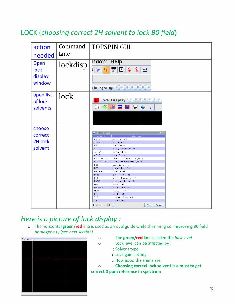
LOCK (choosing correct 2H solvent to lock B0 field)
action needed
Command Line
TOPSPIN GUI
Open lock display window
lockdisp
open list of lock solvents
lock
choose correct 2H lock solvent
Here is a picture of lock display :
o The horizontal green/red line is used as a visual guide while shimming i.e. improving B0 field homogeneity (see next section)
o The green/red line is called the lock level o Lock level can be affected by :
o Solvent type o Lock gain setting o How good the shims are
o Choosing correct lock solvent is a must to get correct 0 ppm reference in spectrum

16
SHIMMING (same as increasing B0 field homogeneity)
action needed
Command Line
TOPSPIN and BSMS GUI
Open the BSMS soft keyboard
bsmsdisp
Perform default automatic shimming (without opening BSMS keyboard)
tune .sx
Here is a picture of Autoshimming tab of BSMS soft keyboard :
o The autoshim function is typically used to maintain the B0 field homeogenity optimal, while running long data collection sessions.
o Examples : o 13C spectra without decoupling
o 1D NOE difference experiments
o T1 measurements on low concentration samples
o AUTOSHIM from BSMS GUI is not always the same as the automated shimming started with “tune .sx” command

17
Here is a picture of bsms soft keyboard:
o You can invoke many more functions, other than the SHIMMING function, from BSMS soft keyboard
o The most important shim gradients for routine shimming can be accessed from the Main tab
o The role played by the knob in BSMS
hardware keyboard is now taken by the buttons
o Shimming Example for Z grad:
To shim on Z, click on the button.
Click on to increase shim value
OR click on to decrease shim current
Try to increase the lock level while you do the above
o Actual shim value is shown here
o Amount of change you made to the shim value
is shown here o From the Main tab, you can EJECT sample or
start or stop SPIN using these buttons

18
PARAMETER OPTIMIZATION
to edit parameters specific to your experiment
Command Line
Topspin GUI
ased
important parameters to check
to access from command line
Topspin GUI
spectral width
sw
center of chemical shift axis
o1p
number of scans
ns
standard pulse and delay lengths
getprosol

19
important parameters to check
command line Topspin GUI
correct receiver gain value
rga
Please remember the following points :
Too high receiver gain will distort the spectrum and show spurious peaks that will look like the real peaks.
Too low a receiver gain will result in poor signal to noise (S/N) ratio. This is due to digitization noise.
Don’t try to guess the optimal ‘rg’ value. Always use the ‘rga’ automatic routine to optimize the receiver gain.
As a general rule, the larger the absolute signal strength from the sample, smaller the ‘rg’ value that is needed.
Optimal receiver gain (‘rg’) value will depend on the following: o Sample concentration i.e. mg/ml (not absolute mg !) o Nuclues studied - 1H is more sensitive than 13C. Therefore, you will need
smaller ‘rg’ value for 1H than 13C. o Sample Temperature – Low sample temperature reduces electronic noise and
increases the absolute NMR magnetization. This means, smaller ‘rg’ at low temperatures.
o How good your shims are – better B0 field homogeneity leads to larger peak heights i.e. larger recorded signal from the probehead.
IMPORTANT : Larger ‘rg’ value does not lead to larger signal to noise ratio. Increasing Receiver gain is similar to increasing Volume dial in a music player. Both

20
the signal (i.e. music level) and noise (i.e. background and hiss) increase by the same amount.
21
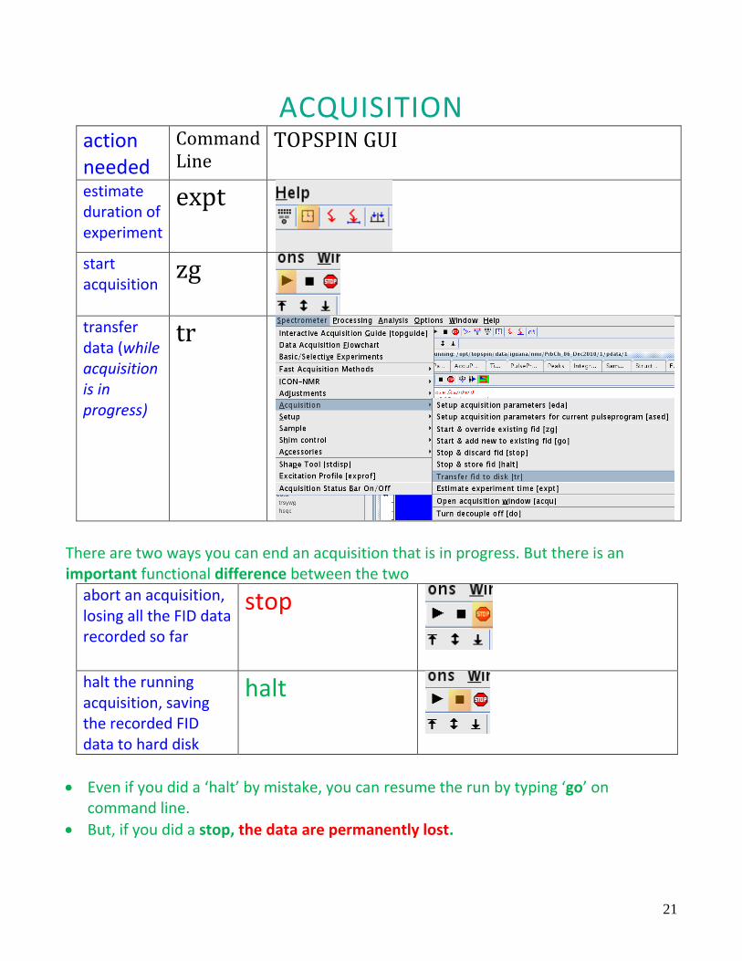
ACQUISITION action needed
Command Line
TOPSPIN GUI
estimate duration of experiment
expt
start acquisition
zg
transfer data (while acquisition is in progress)
tr
There are two ways you can end an acquisition that is in progress. But there is an important functional difference between the two
abort an acquisition, losing all the FID data recorded so far
stop
halt the running acquisition, saving the recorded FID data to hard disk
halt
Even if you did a ‘halt’ by mistake, you can resume the run by typing ‘go’ on command line.
But, if you did a stop, the data are permanently lost.
22
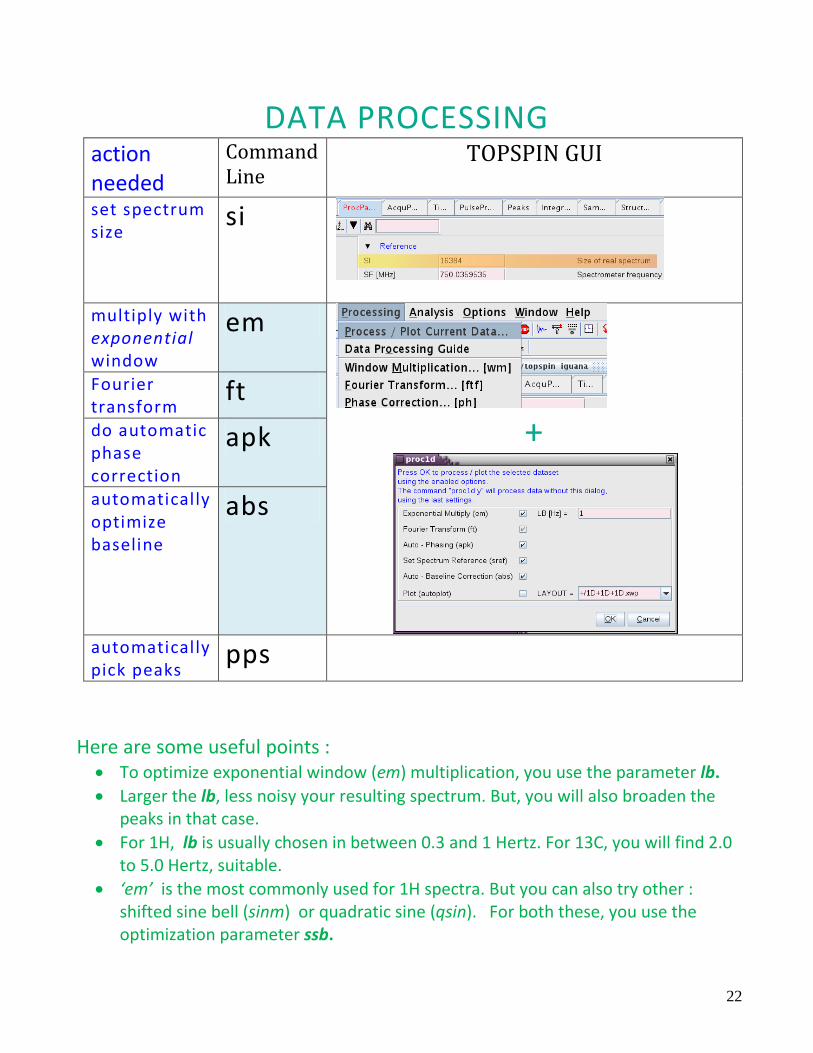
DATA PROCESSING action needed
Command Line
TOPSPIN GUI
set spectrum size
si
multiply with exponential window
em
+
Fourier transform
ft do automatic phase correction
apk
automatically optimize baseline
abs
automatically pick peaks
pps
Here are some useful points :
To optimize exponential window (em) multiplication, you use the parameter lb.
Larger the lb, less noisy your resulting spectrum. But, you will also broaden the peaks in that case.
For 1H, lb is usually chosen in between 0.3 and 1 Hertz. For 13C, you will find 2.0 to 5.0 Hertz, suitable.
‘em’ is the most commonly used for 1H spectra. But you can also try other : shifted sine bell (sinm) or quadratic sine (qsin). For both these, you use the optimization parameter ssb.

23
ssb is set normally 2.0 or above for both sinm and qsin
If you want to separate to close lying peaks clearly, you can use ssb between 1.9 and 2.0.
You can combine em, ft and pk in a single stroke with : efp

24
POST PROCESSING Usually there are only three steps that comprise the post processing part :
Integration
Peak Picking
plotting
INTEGRATION : action needed Command Line TOPSPIN GUI start integration program
.int
OR
Please note these important points about integration : To count number of 1H atoms based on the integrated area i.e. measure
stoichiometry, all the 1H atoms should have nominally the same T1 relaxation times.
This is normally valid for 1H in small molecules in a solution state.
Most other nuclei such as 13C, do not satisfy this condition. So, you cannot integrate a 13C spectrum and compare the areas under different peaks to account for the number of 13C atoms of the molecule.
A clean and flat baseline is important to get reliable integration results.

25
If you have mixture of compounds that differ a lot in their molecular weight, take precautions from ‘over’ interpreting integral results (the individual molecules might have different T1-s).
The following graphic shows the Integration program window and highlights the most commonly used controls and icons.
What the menu items do when you right click under any integral are briefly explained here :
By clicking on this you can select the integral under the
red vertical line. You can select all integrals by using this icon in the tool bar.
When you click here, you get this dialog box in which you can enter the proton stoichiometry standard value for your compound
Resize integral on screen
Change mouse
sensitivity
Save and quit Quit and lose
everything
Cut integral in two
tool
Click and drag tool
tool
Autoscale all integrals to equal height
tool
Right Click under any integral for this
menu
26
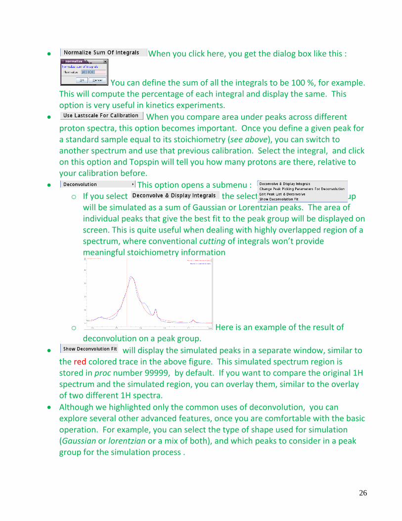
When you click here, you get the dialog box like this :
You can define the sum of all the integrals to be 100 %, for example. This will compute the percentage of each integral and display the same. This option is very useful in kinetics experiments.
When you compare area under peaks across different proton spectra, this option becomes important. Once you define a given peak for a standard sample equal to its stoichiometry (see above), you can switch to another spectrum and use that previous calibration. Select the integral, and click on this option and Topspin will tell you how many protons are there, relative to your calibration before.
This option opens a submenu : o If you select the selected integral i.e. peak group
will be simulated as a sum of Gaussian or Lorentzian peaks. The area of individual peaks that give the best fit to the peak group will be displayed on screen. This is quite useful when dealing with highly overlapped region of a spectrum, where conventional cutting of integrals won’t provide meaningful stoichiometry information
o Here is an example of the result of deconvolution on a peak group.
will display the simulated peaks in a separate window, similar to the red colored trace in the above figure. This simulated spectrum region is stored in proc number 99999, by default. If you want to compare the original 1H spectrum and the simulated region, you can overlay them, similar to the overlay of two different 1H spectra.
Although we highlighted only the common uses of deconvolution, you can explore several other advanced features, once you are comfortable with the basic operation. For example, you can select the type of shape used for simulation (Gaussian or lorentzian or a mix of both), and which peaks to consider in a peak group for the simulation process .
27
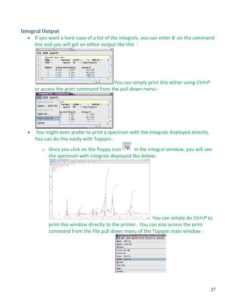
Integral Output If you want a hard copy of a list of the integrals, you can enter li on the command
line and you will get an editor output like this :
You can simply print this either using Ctrl+P or access the print command from the pull down menu :
You might even prefer to print a spectrum with the integrals displayed directly.
You can do this easily with Topspin :
o Once you click on the floppy icon in the integral window, you will see the spectrum with integrals displayed like below:
You can simply do Ctrl+P to print this window directly to the printer. You can also access the print command from the File pull down menu of the Topspin main window :

28
Peak picking: action needed Command Line TOPSPIN GUI start peak picking program
.pp
OR
Please note these important points about peak picking :
Peak picking program tries to identify the ‘point of inflexion’ to recognize a peak i.e. it follows an increasing part of a curve until it stops increasing and then change direction and start decreasing. This crossover point is the definition of a ‘peak’.
Several points of a curve can, in principle, satisfy this definition of a ‘point of inflexion’. Examples include, a shoulder to a main peak, a noisy spike that increases and decreases sharply, or a broad hump in the baseline. How do we then recognize the ‘real’ peaks from artifacts?
Since there is no ‘absolute definition’ possible for a valid NMR peak that a computer program can follow, user assistance will be necessary sometimes.
The parameter pc (also known as peak picking sensitivity), will help the program ignore peaks that are spurious, as decided by the user.
Larger the value of pc, smaller the number of peaks that will be recognized within a given region. The default value of pc is 1.
29
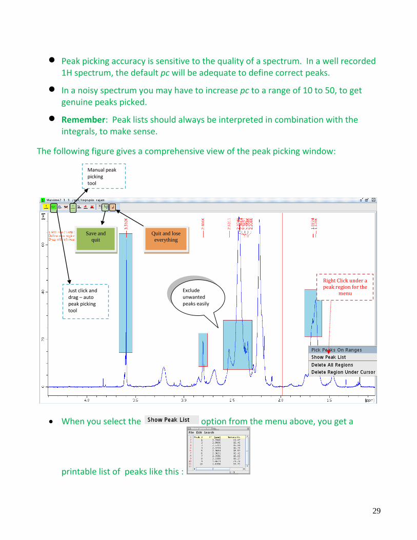
Peak picking accuracy is sensitive to the quality of a spectrum. In a well recorded 1H spectrum, the default pc will be adequate to define correct peaks.
In a noisy spectrum you may have to increase pc to a range of 10 to 50, to get genuine peaks picked.
Remember: Peak lists should always be interpreted in combination with the integrals, to make sense.
The following figure gives a comprehensive view of the peak picking window:
When you select the option from the menu above, you get a
printable list of peaks like this :
Right Click under a peak region for the
menu
Save and
quit
Quit and lose
everything
Just click and drag – auto peak picking tool
Exclude unwanted peaks easily
Manual peak picking tool

30
PLOTTING : There are two ways in which you can generate hard copy output of your spectrum:
You can enter Ctrl+P on the keyboard and print the current view of the spectrum directly. You get the following dialog box
first: You can simply click the OK button
to plot the current view on screen directly :
OR You can start the highly flexible plot editor program by typing:
plot on the command line.
The Plot editor is quite versatile and can generate publication quality soft copies of spectra with annotations and decorations. The plot editor is explained in detail in the following pages.
31
PLOTTING – PLOT EDITOR
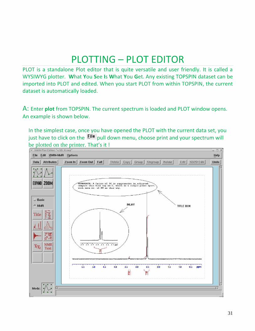
PLOT is a standalone Plot editor that is quite versatile and user friendly. It is called a WYSIWYG plotter. What You See Is What You Get. Any existing TOPSPIN dataset can be imported into PLOT and edited. When you start PLOT from within TOPSPIN, the current dataset is automatically loaded.
A: Enter plot from TOPSPIN. The current spectrum is loaded and PLOT window opens.
An example is shown below.
In the simplest case, once you have opened the PLOT with the current data set, you
just have to click on the pull down menu, choose print and your spectrum will be plotted on the printer. That’s it !

32
B: Optimizing PLOT Features:
PLOT BUTTONS AND THEIR FUNCTIONS:
Select a Graphics Object (Spectrum, Title Box, etc.)
Expand a region of the spectrum using mouse
Zoom onto a region of the display – On Screen only
Insert Title from the current data set
Insert the list of parameters for the current data
Single spectrum display mode
Spectral Array display mode
Text insertion box
Any of the above buttons can be clicked once to choose that particular mode of editing. The mode you have chosen currently, will be displayed in the lower left corner of the plot area, as shown below:
To switch between modes, you have to click the corresponding button once.

33
PLOT shows a “white” area in a cyan background. This is a “virtual sheet of paper” on which you will place your graphics objects.
By default, PLOT includes the following objects of display, when you open it with a valid dataset.
Spectrum in landscape orientation
List of parameters used in a two column format on the right side of the spectrum
Integrals
Title of the spectrum from the dataset. The default behavior can be changed completely by editing the objects of display individually. Do the following for the editing.
1. Click on the button. Move the cursor onto the spectrum display and click once. The spectrum area is surrounded by “green” handles or hot spots, like below.

34
2. Now click on the button on the top right corner, next to the button. You will get an edit window like below:
Edit font type, sizes,
curve thickness, etc.
Size of the spectrum window displayed.
X-axis Units
Size and position of displayed integrals
Re-scale the vertical size of spectrum
Define the ppm range to display

35
1. If you want peaks to be displayed, you can turn on the button. 2. If you want to change the limits of X-axis, you can modify the
range. 3. Similary, to scale the spectrum in vertical direction, modify Y-axis limits, using
entry.
4. Once you are finished, click or
5. If you are happy with the appearance of the spectrum, simply click on pull
down menu and select to print the spectrum. You can edit pretty much any other graphics object that was placed inside the “white” area of PLOT by using the edit mode. Other useful features of the PLOT program you can explore :
You can inlay any number of spectra within the same sheet of paper . This is useful, to expand a small region of a spectrum and show the finer features such as multiplets in more detail.
PLOT program can be used to plot 2D spectra as well. Use the mode button
for the same. Once you import a processed 2D spectrum into the window,
you can select the same and use the button to edit 2D plot features : number of contour levels, contour scale, positive and negative contour levels, etc.
Stack plots, that display a number of 1D spectra in a series can be plotted with PLOT program. This is typically used to show evolution of a given peak in kinetics experiments or to show the relaxation recovery profile in T1 and T2
experiments. Use the mode button to access this feature.
If your dataset contains the processed pseudo-2D data such as T1 or T2, you can
use the mode to plot the recovery curve along with a spectrum, for instance.
You can annotate your spectral features with text of your choice. Click on the
mode button and you will be presented with a text window. You can place this window where you need and type in the contents.

36
CLEANUP
Last but not the least are the final steps listed below. These are very important to follow so that the next user gets the spectrometer in a predictable, stable and standard condition to set up her/his experiments. Remember, YOU could be that next user !
Stop spinning the sample, if you used spinning before.
Turn off lock
Lift the sample
Set the temperature to 298 K
If you had used an X-nucleus (for observe or decouple), set the X-channel to 13C in a tuned/matched condition.
Insert the dummy sample that is kept next to the spectrometer.
Type exit at the command line and answer ‘Yes’ to all questions.

37
This will close the Topspin program properly and log you out.
REMINDER :
Please remember that, until you logout of the system completely, your UWNetid login will be still alive.
Other than being a security risk, this can give an unknown user, the privilege to access your data and even accidental deletion of the same.
It is therefore imperative that you logout after your turn is done.

38
APPENDIX A dot commands: Topspin provides several dialog box interfaces
as well as graphical interfaces to perform tasks. With some commands, whether you start a dialog box or a graphical interface for a given task is decided by ‘prefixing’ a “.” to the same command name. Example:
.int starts the graphical integration window where you can perform interactive integration
int (without the dot) brings up a dialog box like this :
Here are some dot commands and their ordinary counterparts, for quick reference:
dot command
function non-dot command
function
.int open integration graphical window
int dialog box to set parameters for non-interactive integration
.pp open interactive peak picking window
pp peak picking dialog box to optimize automatic peak picking
.cal open interactive 0 ppm referencing window
cal dialog box to choose automatic or manual spectrum calibration
.ph open interactive phase correction window
ph dialog box to optimize automatic phase correction
keyboard shortcuts: Several routine operations can be done

39
quickly by a combination of key strokes. Example: Ctrl+P prints the currently displayed spectrum window in the printer. Here are some keyboard shortcuts :
Key stroke combination function
Ctrl + N Open dialog box to create new data set
Ctrl + O Open NMR existing dataset - dialog box appears
Ctrl + W close current dataset
Ctrl + S open a wrpa dialog box – save data in different formats
Ctrl + P print dialog box
Ctrl + F Find a specific dataset – dialog box
Ctrl + D File Browser Panel – on/off
40
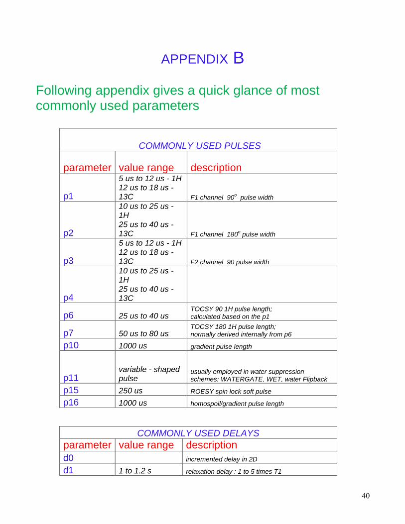
APPENDIX B Following appendix gives a quick glance of most commonly used parameters
COMMONLY USED PULSES
parameter value range description
p1
5 us to 12 us - 1H 12 us to 18 us - 13C F1 channel 90
o pulse width
p2
10 us to 25 us - 1H 25 us to 40 us - 13C F1 channel 180
o pulse width
p3
5 us to 12 us - 1H 12 us to 18 us - 13C F2 channel 90 pulse width
p4
10 us to 25 us - 1H 25 us to 40 us - 13C
p6 25 us to 40 us TOCSY 90 1H pulse length; calculated based on the p1
p7 50 us to 80 us TOCSY 180 1H pulse length; normally derived internally from p6
p10 1000 us gradient pulse length
p11 variable - shaped pulse
usually employed in water suppression schemes: WATERGATE, WET, water Flipback
p15 250 us ROESY spin lock soft pulse
p16 1000 us homospoil/gradient pulse length
COMMONLY USED DELAYS
parameter value range description
d0 incremented delay in 2D
d1 1 to 1.2 s relaxation delay : 1 to 5 times T1

41
COMMONLY USED DELAYS
parameter value range description
d2 J for CH: 125 to 222 Hz 1/2J
d3 1/3J
d4 1/4J : used in HSQC
d6 delay for evolution of long range couplings
d7 delay for inversion recovery
d8 200 ms to 1 s NOESY mixing time
d9 60 ms to 80 ms TOCSY mixing time
d11 30 ms : default delay for disk I/O
d12 20 us : default delay for power switching
d14 delay for evolution after shaped pulse.
d16 200 to 500 us delay for gradient recovery
d19 100 to 200 us
delay for binomial water suppression in WATERGATE : 1/[2*d19] gives the position of next null
COMMONLY USED CONSTANTS
parameter significance description
cnst0 used in different contexts.
cnst1 J (HH) proton-proton J coupling stored as default
cnst2 J (XH) ex: proton-carbon 1 bond J coupling
cnst3 J (XX) ex: carbon-carbon 1 bond J coupling in labeled solute
cnst11 1 or 2 for multiplicity selection in DEPT or APT
cnst12 1 or 2 for multiplicity selection
42
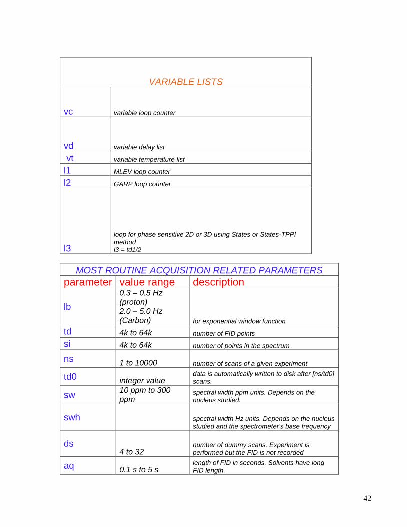
VARIABLE LISTS
vc variable loop counter
vd variable delay list
vt variable temperature list
l1 MLEV loop counter
l2 GARP loop counter
l3
loop for phase sensitive 2D or 3D using States or States-TPPI method l3 = td1/2
MOST ROUTINE ACQUISITION RELATED PARAMETERS
parameter value range description
lb
0.3 – 0.5 Hz (proton) 2.0 – 5.0 Hz (Carbon) for exponential window function
td 4k to 64k number of FID points
si 4k to 64k number of points in the spectrum
ns 1 to 10000 number of scans of a given experiment
td0 integer value data is automatically written to disk after [ns/td0] scans.
sw 10 ppm to 300 ppm
spectral width ppm units. Depends on the nucleus studied.
swh
spectral width Hz units. Depends on the nucleus studied and the spectrometer's base frequency
ds 4 to 32
number of dummy scans. Experiment is performed but the FID is not recorded
aq 0.1 s to 5 s length of FID in seconds. Solvents have long FID length.
43
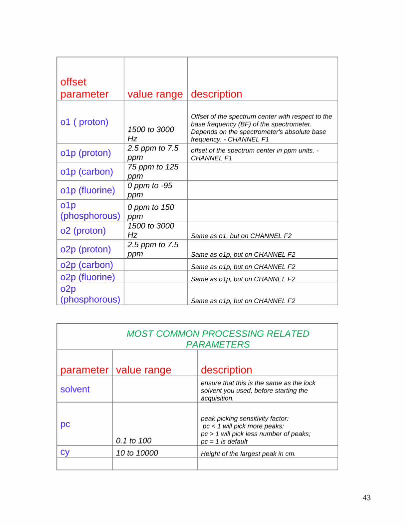
offset parameter value range description
o1 ( proton) 1500 to 3000 Hz
Offset of the spectrum center with respect to the base frequency (BF) of the spectrometer. Depends on the spectrometer's absolute base frequency. - CHANNEL F1
o1p (proton) 2.5 ppm to 7.5 ppm
offset of the spectrum center in ppm units. - CHANNEL F1
o1p (carbon) 75 ppm to 125 ppm
o1p (fluorine) 0 ppm to -95 ppm
o1p (phosphorous)
0 ppm to 150 ppm
o2 (proton) 1500 to 3000 Hz Same as o1, but on CHANNEL F2
o2p (proton) 2.5 ppm to 7.5 ppm Same as o1p, but on CHANNEL F2
o2p (carbon) Same as o1p, but on CHANNEL F2
o2p (fluorine) Same as o1p, but on CHANNEL F2
o2p (phosphorous) Same as o1p, but on CHANNEL F2
MOST COMMON PROCESSING RELATED PARAMETERS
parameter value range description
solvent
ensure that this is the same as the lock solvent you used, before starting the acquisition.
pc
0.1 to 100
peak picking sensitivity factor: pc < 1 will pick more peaks; pc > 1 will pick less number of peaks; pc = 1 is default
cy 10 to 10000 Height of the largest peak in cm.
44
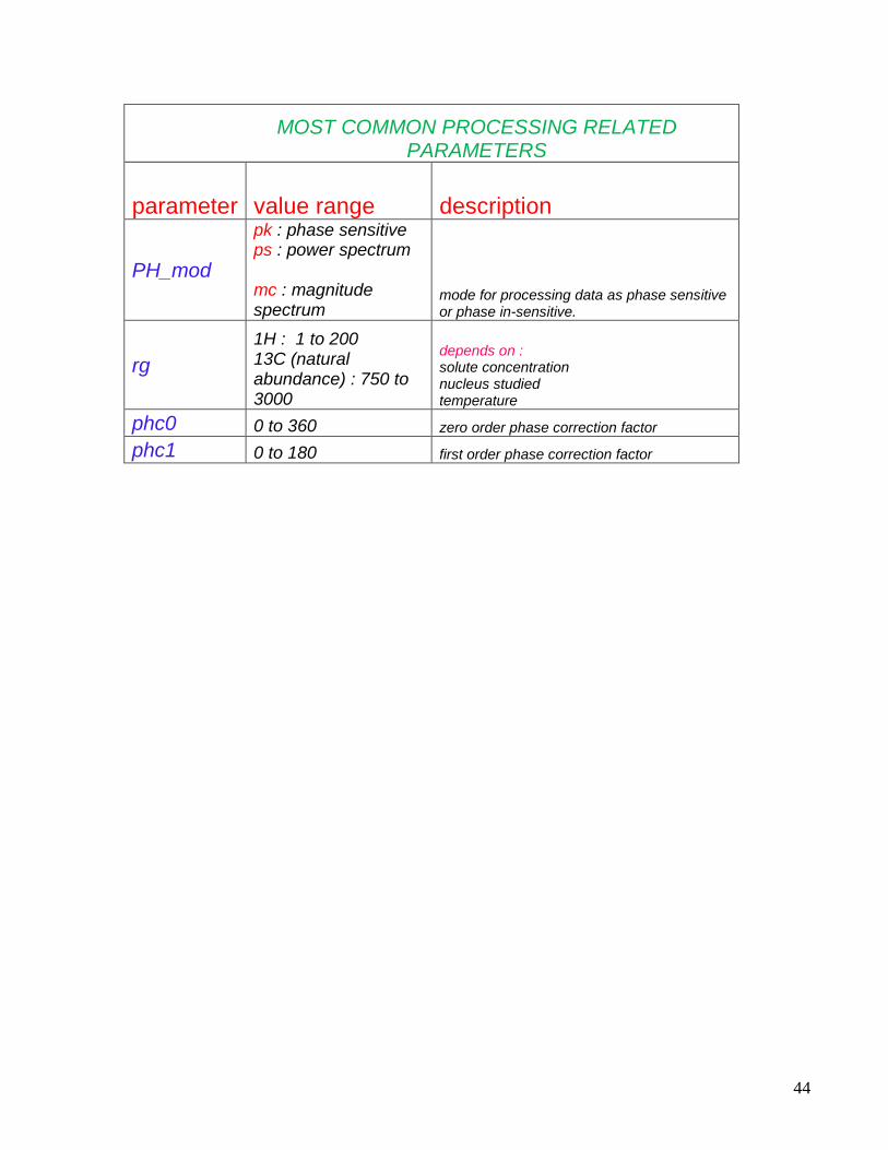
MOST COMMON PROCESSING RELATED PARAMETERS
parameter value range description
PH_mod
pk : phase sensitive ps : power spectrum mc : magnitude spectrum
mode for processing data as phase sensitive or phase in-sensitive.
rg
1H : 1 to 200 13C (natural abundance) : 750 to 3000
depends on : solute concentration nucleus studied temperature
phc0 0 to 360 zero order phase correction factor
phc1 0 to 180 first order phase correction factor
45
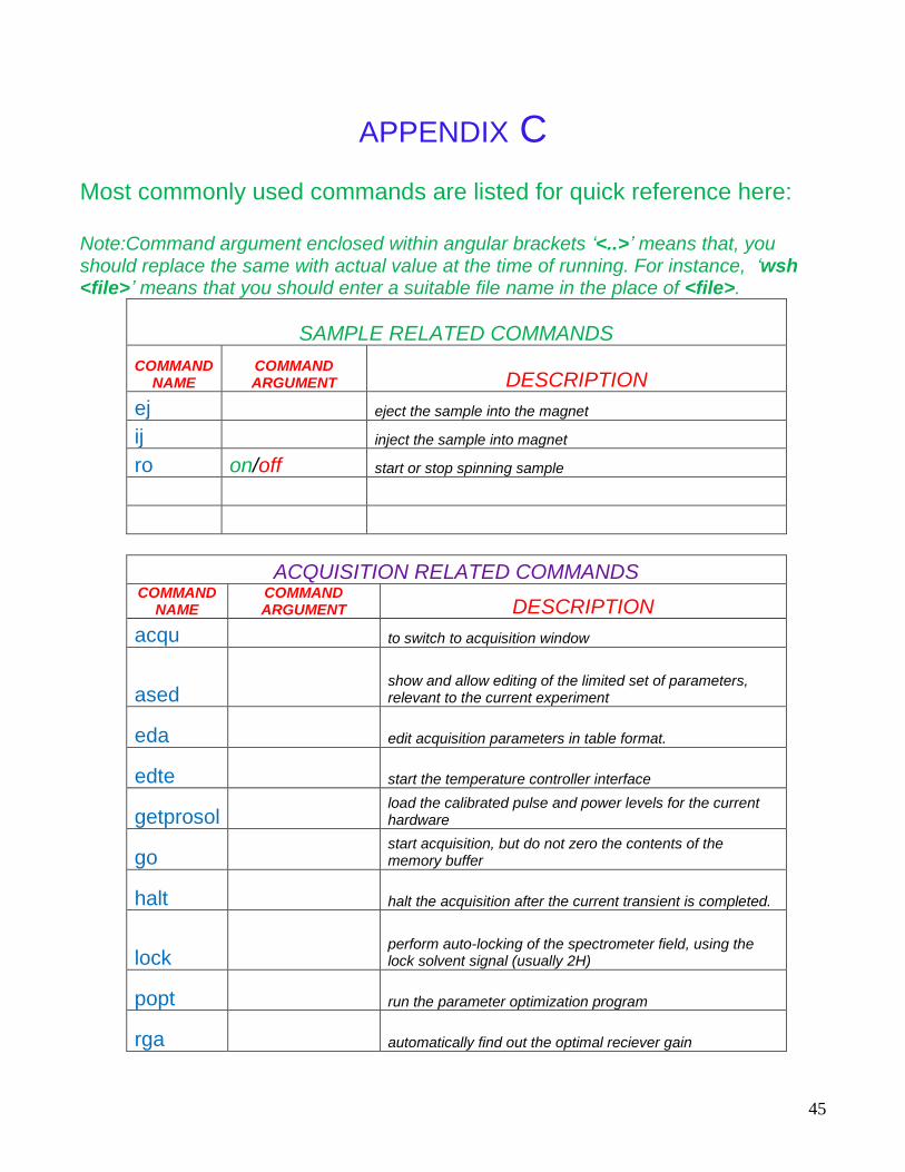
APPENDIX C Most commonly used commands are listed for quick reference here: Note:Command argument enclosed within angular brackets ‘<..>’ means that, you should replace the same with actual value at the time of running. For instance, ‘wsh <file>’ means that you should enter a suitable file name in the place of <file>.
SAMPLE RELATED COMMANDS
COMMAND NAME
COMMAND ARGUMENT DESCRIPTION
ej eject the sample into the magnet
ij inject the sample into magnet
ro on/off start or stop spinning sample
ACQUISITION RELATED COMMANDS COMMAND
NAME COMMAND ARGUMENT DESCRIPTION
acqu to switch to acquisition window
ased show and allow editing of the limited set of parameters, relevant to the current experiment
eda edit acquisition parameters in table format.
edte start the temperature controller interface
getprosol load the calibrated pulse and power levels for the current hardware
go start acquisition, but do not zero the contents of the memory buffer
halt halt the acquisition after the current transient is completed.
lock perform auto-locking of the spectrometer field, using the lock solvent signal (usually 2H)
popt run the parameter optimization program
rga automatically find out the optimal reciever gain
46
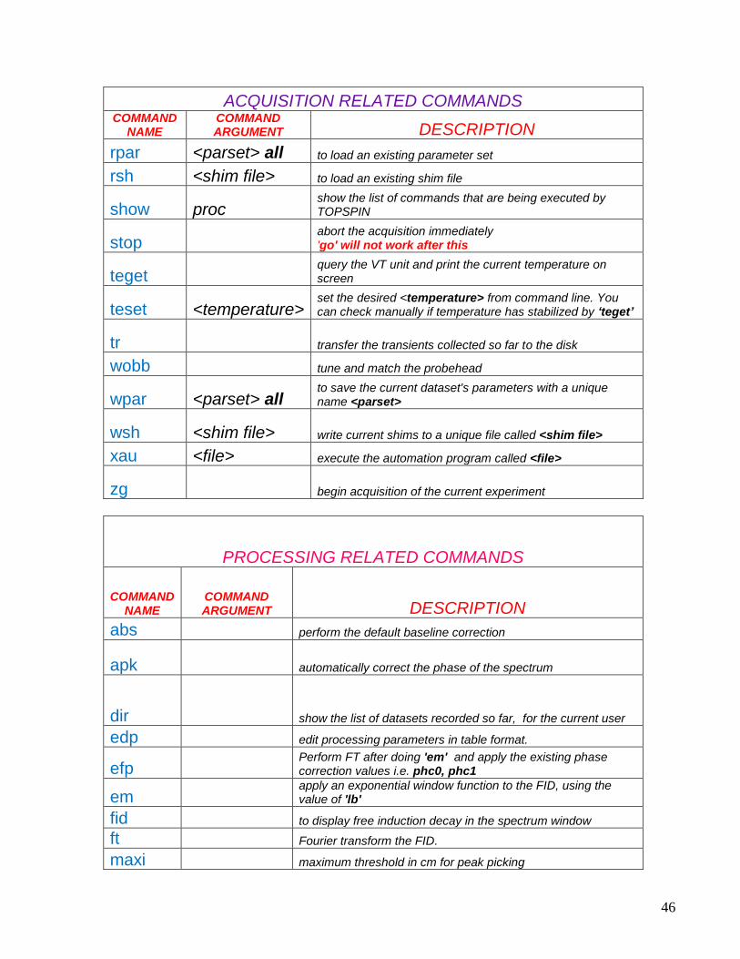
ACQUISITION RELATED COMMANDS COMMAND
NAME COMMAND ARGUMENT DESCRIPTION
rpar <parset> all to load an existing parameter set
rsh <shim file> to load an existing shim file
show proc show the list of commands that are being executed by TOPSPIN
stop abort the acquisition immediately 'go' will not work after this
teget query the VT unit and print the current temperature on screen
teset <temperature> set the desired <temperature> from command line. You can check manually if temperature has stabilized by „teget‟
tr transfer the transients collected so far to the disk
wobb tune and match the probehead
wpar <parset> all to save the current dataset's parameters with a unique name <parset>
wsh <shim file> write current shims to a unique file called <shim file>
xau <file> execute the automation program called <file>
zg begin acquisition of the current experiment
PROCESSING RELATED COMMANDS
COMMAND NAME
COMMAND ARGUMENT DESCRIPTION
abs perform the default baseline correction
apk automatically correct the phase of the spectrum
dir show the list of datasets recorded so far, for the current user
edp edit processing parameters in table format.
efp Perform FT after doing 'em' and apply the existing phase correction values i.e. phc0, phc1
em apply an exponential window function to the FID, using the value of 'lb'
fid to display free induction decay in the spectrum window
ft Fourier transform the FID.
maxi maximum threshold in cm for peak picking

47
PROCESSING RELATED COMMANDS
COMMAND NAME
COMMAND ARGUMENT DESCRIPTION
mi minimum threshold in cm for peak picking
plot
launch PLOT plot editor opens the editor, with the current dataset for display, as a default.
pps display the picked peak list on screen.
re m n
switch to a different [Exp. No, Proc. No.] combination of the current data set. m : experiment number n: processed data number
setti open an editor for creating a title for the current dataset.
sino calculate the signal to noise ratio you must define the signal and noise regions prior to this.
sref automatically perform spectrum calibration based on lock solvent and TMS info.
wm enter manual window function manipulation program
wra m
copy the raw data (FID) from the current experiment number to a different one. m: experiment number
wrp n
copy the current processed spectrum to a different proc.number within the same dataset n: processed data number
wrpa m n
copy the current dataset in its entirety (including the FID and the spectrum) to a new [Exp. No, Proc. No.] combination. m : experiment number n: processed data number