Non-centralized Control for Flow-based Distribution

Networks: A Game-theoretical Insight

Julian Barreiro-Gomez a,b, Carlos Ocampo-Martinez a, Nicanor Quijano b, andJose M. Maestre c

aAutomatic Control Department, Universitat Politecnica de Catalunya, Institut de Robotica i Informatica Industrial(CSIC-UPC), Llorens i Artigas, 4-6, 08028 Barcelona, Spain

bDepartamento de Ingenierıa Electrica y Electronica, Universidad de los Andes, Carrera 1 No 18A-10, Bogota, Colombia

cDepartamento de Ingenierıa de Sistemas y Automatica, Universidad de Sevilla, 41092 Sevilla, Spain

Abstract

This paper solves a data-driven control problem for a flow-based distribution network with two objectives: a resource allocationand a fair distribution of costs. These objectives represent both cooperation and competition directions. It is proposed asolution that combines either a centralized or distributed cooperative game approach using the Shapley value to determinea proper partitioning of the system and a fair communication cost distribution. On the other hand, a decentralized non-cooperative game approach computing the Nash equilibrium is used to achieve the control objective of the resource allocationunder a non-complete information topology. Furthermore, an invariant-set property is presented and the closed-loop systemstability is analyzed for the non-cooperative game approach. Another contribution regarding the cooperative game approachis an alternative way to compute the Shapley value for the proposed specific characteristic function. Unlike the classicalcooperative-games approach, which has a limited application due to the combinatorial explosion issues, the alternative methodallows calculating the Shapley value in polynomial time and hence can be applied to large-scale problems.

Key words: Flow-based distribution networks, population games, Nash equilibrium, cooperative games, Shapley value,dynamic resource allocation, partitioning approach, distributed control.

1 Introduction

The ideal centralized control scheme in which a single entity governs a system using full information, disposing ofenough time to gather all the measurements, and to compute and transmit all the control inputs, may not be realisticfor certain systems. Real large-scale control problems usually present issues that limit the application of centralizedcontrol strategies, e.g., fast dynamics with demanding response times, unavailability of full information, intractabilityof the problem due to its sheer size, among others. These issues are of special interest in the control field and agreat effort has been placed into the development of non-centralized control techniques in order to mitigate them.In addition, significant technological changes have occurred during the last decades that have modified the waythese problems are addressed. This is particularly visible if the methods used some decades ago [34] are comparedwith those used today [17]. Nowadays, computing and networking elements are pervasive and state-of-the-art controltechniques are more and more sophisticated to take advantage of the new possibilities that technology offers.

This paper focuses on one of the recent trends in the development of non-centralized control techniques. In particular,during the last years different control strategies, which are able to adapt dynamically to the evolution of the system

Email addresses: j.barreiro135@uniandes.edu.co - jbarreiro@iri.upc.edu (Julian Barreiro-Gomez),cocampo@iri.upc.edu (Carlos Ocampo-Martinez), nquijano@uniandes.edu.co (Nicanor Quijano), pepemaestre@us.es(Jose M. Maestre).

under control and its structure, have been presented. For example, in [25] it is proposed a suitable on-line methodto decide which information should be shared and used between different local predictive controllers operating withvarious topologies. In [33], plug-and-play decentralized model predictive controllers are studied. In [14], a method todesign simultaneously the communication topology and feedback control laws is proposed. Likewise in [18], a controlmethod that switches between different linear feedback controllers to attain a trade-off between communicationburden and performance is proposed. This latter work has been extended to the model predictive framework in [7].The rationale of this work is somehow similar to [18] since the control architecture changes its topology in order toreduce the communication burden. However, unlike the aforementioned works, the control strategy proposed in thiswork uses both a cooperative and a non-cooperative game-theory approaches. Game theory has become a powerfultool in the design of learning and optimization-based systems [4][19][31]. Both cooperative and non-cooperativegame approaches have been widely used in the design of controllers depending on their control objectives. In somecases, it is more suitable to work with a cooperative perspective when agents can collaborate among them, whereasthere are other situations in which it is more appropriate to state the problem as a competition. However, there arecontrol problems that integrate both cooperation and competition in two different stages. Furthermore, the proposedapproach is a data-driven control inspired by the dynamic resource allocation problem [1][29].

Another contribution of this paper is to deepen into the relationship between game theory and control. Being themathematical field that deals with situations of mutual interaction [22], game theory has a natural application inthe context of non-centralized controllers. Broadly speaking, game theory has two main branches depending onwhether the players of the game are capable to cooperate with each other or not. In particular, non-cooperativegame theory deals with problems where players make decisions to maximize their utilities. A typical outcome ofa non-cooperative game is given by the Nash equilibrium, condition in which no player can improve their utilitieswithout the detriment of the utility of other players. In order to solve the non-cooperative game, it is proposed theuse of population games, e.g., replicator, projection, Smith, Brown-Von-Neumann-Nash, best response, and logitchoice dynamics [35]. In contrast, cooperative game theory studies the conditions and payoff rules for groups ofplayers that form coalitions. A solution of a cooperative game is given by the Shapley value, which assigns a fairpayoff to each player according to its contribution. There are several control solutions that use both game theoryapproaches. For instance in [16], an application of non-cooperative game theory can be found, where a distributedcontrol strategy based on the convergence to a Nash equilibrium is proposed [24]. Furthermore, convergence to Nashequilibrium by using evolutionary-game theory has been used in the design of control and optimization strategies[3][26][39]. On the other hand, cooperative game theory has been used for example in [6], where a coalitional controlapproach is introduced, or in [18], where a control scheme considering different network topologies is presented. Inthis and other related works such as [21], the links that compose the network topology are transformed into theplayers of a game and the payoff given by the Shapley value is used as a mean to determine the relevance of the links[37]. Other works that mainly use the Shapley value are [10], and [15]. In [10] the Shapley value as a distribution ruleis used to guarantee the existence of a Nash equilibrium in any game. In [15] an evolutionary coalitional approachis proposed so that entities can decide in an autonomous manner whether it is profitable or not to make a coalition.

Several engineering problems may be addressed as a flow-based distribution network as discussed in [11]. In thispaper, a specific flow-based distribution network is considered, and a combination of two game-theoretical approachesis used to propose a decentralized control strategy (i.e., population and cooperative games). The incentives of theaforementioned combination are given by the fact that the control problem involves both competition and cooperationin two different objectives, i.e., competition in a dynamical resource allocation problem, and cooperation in the fairdistribution of communication costs. More specifically, the flow-based distribution network is divided into differentpartitions. These partitions are determined by a criterion based on a cooperative game, i.e., by using the Shapleyvalue. Unlike [20], where the Shapley value is computed by considering weights of the links in a complete graph,this paper proposes the use of the error with respect to the maximum capacity of storage elements in the network.Furthermore, a population-game approach is implemented at each partition to solve the resource allocation problemwithout using a complete information topology. Then, a data-driven dynamic resource allocation problem is solvedat each sub-system by converging to a Nash equilibrium. The stability of the closed-loop system, composed of theflow-based distribution network and the population games, is analyzed by using passivity theory as in [1][8][30][32].Moreover, this paper proposes a different way to compute the Shapley value for a specific characteristic functionin the cooperative game in order to reduce the computational burden, which is one of the main issues when usingthis game-theoretical approach. Unlike the classical cooperative-games approach, which has a limited applicationdue to the combinatorial explosion issues, the alternative method allows calculating the Shapley value in polynomialtime and hence can be applied to large-scale problems. Besides, the considerable reduction in the computationalcost also allows computing the Shapley value in a distributed way. Finally, in order to show the performance of theproposed methodology based on cooperative and non-cooperative games, a resource allocation problem in a watersystem treated in [32] is presented. Different from the preliminary work presented in [2], this paper includes analysis

2

regarding invariant-set properties that guarantee a limitation resource constraint, and the stability of the wholeclosed-loop system. The resource allocation problem has been addressed with replicator and projection dynamicssince they share some important gradient characteristics, which have been studied in [36]. Besides, it is discussedthe fact that the main result related to the cooperative game approach allows to compute the Shapley value under adistributed structure, i.e., without considering a complete graph connecting the whole set of players. Also, it is shownthat this result leads to an additional alternative to compute the Shapley value by using a linear set of equations andusing the coalitional rationality axiom (in a centralized manner, or under a distributed structure). As a consequenceof the decrement of required communication links to make the computation under distributed structures, there isan increment in the computational cost. However, a comparison between three alternatives to compute the Shapleyvalue, including the computation under a distributed structure, has been added in function of the number of players.This comparison shows that the computation under a distributed structure is faster with respect to the traditionalcomputation of the Shapley value as there is an increment in the number of players.

The remainder of this paper is organized as follows. Section 2 presents the flow-based distribution network and thecorresponding control objectives for a resource allocation problem. In addition, it is shown that the considered flow-based distribution network is passive. Section 3 presents the population-games approach used to find the solutiongiven by the Nash equilibrium. Replicator and projection dynamics are also introduced. Afterwards, it is shownthat these dynamics satisfy invariance of the simplex set, and that the population games are lossless. Besides,the stability analysis of the closed loop with the flow-based distribution network and the population dynamics ispresented. In Section 4, the role of the cooperative-game approach in a particular control problem is shown. Thiscooperative direction is addressed by finding the solution given by the Shapley value. This section also presentsthe distributed computation of the Shapley value, including a comparison among the computational burden for thedifferent methodologies used. Also, the partitioning is performed using the Shapley value. Section 5 describes a waterdistribution network as a case study and the related control objectives. Besides, results for three different sizes ofpartitions are discussed. Finally, concluding remarks are drawn in Section 6.

Notation:

Column vectors are denoted by bold style, e.g., x. Matrices are denoted by upper case bold style, e.g., A. Scalarnumbers are denoted by non-bold style, e.g., N . Sets are denoted by calligraphic upper case, e.g., T . Sub-indexrefers to the topologies in the system, and super-index refers to partitions, e.g., Vji refers to a set of a partition j ofa topology i. It is worth to point out that super-index is not operational, i.e, N3

i refers to partition 3, and not toNiNiNi. Real numbers are denoted by R, and all the non-negative real numbers by R≥0. Positive integer numbersare denoted by Z>0. The column tile with N unitary entries is denoted by 1N , and the cardinality of set is definedby | · |, e.g., |O| is the amount of elements of the set O. Finally, the time dependency in most of the variables isomitted throughout this paper to simplify the notation.

2 Problem Statement in Distribution Flow-based Networks

Several engineering problems may be addressed as a flow-based distribution network just by defining general elementssuch as suppliers and demands, flow capacity, and storage capacity [11]. Consider a specific resource flow-baseddistribution network, which is composed of three types of elements:

• Storage: element that stores the resource and with both inflows and outflows. Let V = {1, . . . , N} be the set ofN ∈ Z>0 storage nodes 1 .• Sink: element that receives the resource from a storage node and with only inflows. Let B = {N + 1, . . . , 2N} be

the set N ∈ Z>0 of sink nodes.• Source: element that provides the resource and with only outflows. Let R = {2N + 1} be the singleton set of a

source node.

Consider a directed graph denoted by G = (V, E), where V = {V ∪ B ∪ R} is the set of 2N + 1 nodes representing

the storage, sink, and source elements in the flow-based distribution network, and E ⊂ {(r, `) : r, ` ∈ V} is the set of

1 The set V has three different interpretations depending on the context in which it is used, i.e.,(1) V is the set of N storage nodes in the distribution flow-based networks context (Section 2).(2) V is the set of N strategies in the population-games context (Section 3).(3) V is the set of N players in the cooperative-games context (Section 4).

3

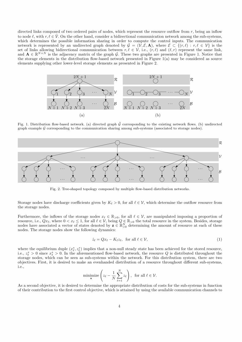
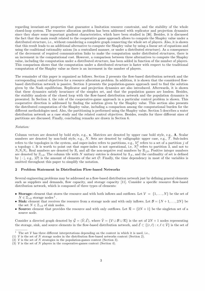
directed links composed of two ordered pairs of nodes, which represent the resource outflow from r, being an inflowto node `, with r, ` ∈ V. On the other hand, consider a bidirectional communication network among the sub-systems,which determines the possible information sharing in order to compute the control inputs. The communicationnetwork is represented by an undirected graph denoted by G = (V, E ,A), where E ⊂ {(r, `) : r, ` ∈ V} is theset of links allowing bidirectional communication between r, ` ∈ V, i.e., (r, `) and (`, r) represent the same link,and A ∈ RN×N is the adjacency matrix of the graph G. These two graphs are presented in Figure 1. Notice thatthe storage elements in the distribution flow-based network presented in Figure 1(a) may be considered as sourceelements supplying other lower-level storage elements as presented in Figure 2.

2N

. . .

N + 2 N + 3N + 1

2 3 N. . .

1

2N + 1

B

V

R

2N

. . .

N + 2 N + 3N + 1

2 3 N. . .

1

2N + 1

B

V

R

(a) (b)

Fig. 1. Distribution flow-based network. (a) directed graph G corresponding to the existing network flows. (b) undirectedgraph example G corresponding to the communication sharing among sub-systems (associated to storage nodes).

. . .

. . .

. . .

. . .

. . .

. . .B

V

R

. . . . . .

Fig. 2. Tree-shaped topology composed by multiple flow-based distribution networks.

Storage nodes have discharge coefficients given by K` > 0, for all ` ∈ V, which determine the outflow resource fromthe storage nodes.

Furthermore, the inflows of the storage nodes x` ∈ R>0, for all ` ∈ V, are manipulated imposing a proportion ofresource, i.e., Qx`, where 0 < x` ≤ 1, for all ` ∈ V, being Q ∈ R>0 the total resource in the system. Besides, storagenodes have associated a vector of states denoted by z ∈ RN>0 determining the amount of resource at each of thesenodes. The storage nodes show the following dynamics:

z` = Qx` −K`z`, for all ` ∈ V, (1)

where the equilibrium duple (x∗` , z∗` ) implies that a non-null steady state has been achieved for the stored resource,

i.e., z∗` > 0 since x∗` > 0. In the aforementioned flow-based network, the resource Q is distributed throughout thestorage nodes, which can be seen as sub-systems within the network. For this distribution system, there are twoobjectives. First, it is desired to make an evenhanded distribution of a resource throughout different sub-systems,i.e.,

minimizex

(z` −

1

N

N∑`=1

z`

), for all ` ∈ V.

As a second objective, it is desired to determine the appropriate distribution of costs for the sub-systems in functionof their contribution to the first control objective, which is attained by using the available communication channels to

4

coordinate the distribution of the resource. The communication cost in an time interval [t0, tf ] associated to the use

of G = (V, E ,A) is given by ϕlinks = 12

∫ tft01>NA1N dt. As a second objective, the fair cost L` that the `th sub-system

should pay for using the communication network must be found. It should be satisfied that∑`∈V L` = ϕlinks.

Finally, assume that the communication graph can have T different topologies from the set T = {1, . . . , T}.Moreover, each topology i ∈ T has Pi different partitions from the set Pi = {1, . . . , Pi}, where each partition

j ∈ Pi of the topology i ∈ T is a complete undirected graph denoted by Gji = (Vji , Eji , ·), where Vji is the set of

N ji storage nodes within the corresponding partition, and Eji = {(r, `) : r, ` ∈ Vji } is the set of links representing the

full-information within each partition. Besides, each partition j ∈ Pi of the topology i ∈ T represents a sub-systemdenoted by Σj

i , which has a disjoint controller denoted by Γji as presented in Figure 3.

Σji

Γji

zjixji

Fig. 3. Closed loop for the sub-system corresponding to partition j ∈ Pi of the topology i ∈ T .

The two different control objectives are achieved by using a game-theoretical approach in a distributed manner. Thefirst control objective associated to an evenhanded distribution of the resource is reached with a non-cooperativeapproach. In contrast, the determination of the fair distribution of costs for all the sub-systems is made with acooperative game approach. Furthermore, suppose that the topology of the communication graph can be reconfiguredconveniently to achieve the control objectives every time τ > 0 (this fact is discussed in Section 3).

A feature of the flow-based distribution network is its passivity property. Lemma 1 presents this property as in [1][8].

Lemma 1 The storage model of the flow-based distribution network Σji in Figure 3 is passive defining its inputs as

the error ez` = z` − z∗` , and its outputs as the error ex`= x` − x∗` , for all ` ∈ Vji , and for all partitions j ∈ Pi of the

topology i ∈ T .

Proof: The proof is presented in the Appendix. �

3 Population Games

Consider a population composed of a finite and large number of rational agents that make the decisions to selectamong a set of possible strategies V = {1, . . . , N} (each strategy associated to a storage node, see Section 2). Agentschange the strategy to improve their utilities or benefits.

Within the population there are T ∈ Z>0 possible different topologies given by a graph that determine how thepopulation structure is configured, i.e., how the agents can interact among them. The set of the population topologiesis denoted by T = {1, ..., T}. Each topology i ∈ T is given by a non–complete graph denoted by Gi = (V, Ei,Ai),where V is the set of N nodes representing the strategies, the set of links that represent the possible interaction amongagents selecting the corresponding strategies is denoted by Ei, and Ai is the adjacency matrix of the correspondingtopology.

Each topology i ∈ T has Pi ∈ Z>0 disjoint partitions. The set of partitions of the population topology i ∈ T is givenby Pi = {1, ..., Pi}. The partition j ∈ Pi of the topology i ∈ T is denoted by a complete graph Gji = (Vji , Eji , ·),where Vji is the set of N j

i < N nodes representing the set of strategies within the corresponding partition Vji ⊂ V, and

Eji is the set of N ji (N j

i − 1)/2 links representing the full-information sharing and interaction within each partition.

Furthermore, it must be satisfied that all the partitions form the entire topology, i.e.,⋃j∈Pi

Gji = Gi, for all i ∈ T .

In the population, the scalar x` ∈ R≥0 is the proportion of agents selecting the strategy ` ∈ V. The vector x ∈ RN≥0 is apopulation state or a strategic distribution composed of all the proportion of agents selecting the available strategies.

5

The set of all the possible population states is given by a simplex denoted by ∆ ={x ∈ RN≥0 : x>1N = 1

}. Similarly,

xji,` ∈ R≥0 is the proportion of agents selecting the strategy ` ∈ Vji available in the partition j ∈ Pi of the topology

i ∈ T . The vector xji ∈ RNji

≥0 is the strategic distribution of agents in the partition j ∈ Pi of the topology i ∈ T .

Finally, let mji be the total mass in the partition j ∈ Pi of the topology i ∈ T given by mj

i = xji>1Nj

i. Since

partitions are disjoint, then∑j∈Pi

mji = 1.

The payoff that agents receive for selecting a particular strategy is given by a fitness function f` : ∆ 7→ R, forthe associated strategy ` ∈ V. The vector of fitness functions in the population is denoted by f and is composedof all the fitness functions f`(x), ` ∈ V. Similarly, the vector of fitness functions of the partition j ∈ Pi of the

topology i ∈ T is denoted by f ji , which is composed of all the fitness functions f`(x), ` ∈ Vji . The average fitnessfunction in the population is given by f = x>f . The average fitness for each partition of each topology is given by

f ji =(xji>

f ji

)/mj

i , j ∈ Pi, i ∈ T , and the average fitness vector for the partition j ∈ Pi of the topology i ∈ T is

f ji = 1Njif ji .

The framework proposed in this paper is given by stable games, which establish conditions over the fitness functionsfor control design. The condition of stable games stated in Definition 1 allows proving asymptotic convergence tothe solution in the non-cooperative game approach addressed by population games as presented in Section 3.2.

Definition 1 (Adapted from [12]) f is a stable game if the Jacobian matrix Df is negative semi-definite with respectto the tangent space denoted by ∆T = {z ∈ RN : z>1N = 0}, i.e., z>Df z ≤ 0, for all z ∈ ∆T , x ∈ ∆.Alternatively, (w − x)>(f(w)− f(x)) ≤ 0, for all x,w ∈ ∆. ♦

In this paper, both replicator and projection dynamics are used [35]. These two population dynamics are especiallyappealing since they have gradient properties that are discussed in [36].

3.1 Replicator and Projection Dynamics

For a fixed topology, there is a replicator dynamics system for each partition. For a topology i ∈ T and a partitionj ∈ Pi, the replicator dynamics introduced in [38] are given by

xji = diag(xji

)(f ji − f ji

), (2)

and the projection dynamics introduced in [23] are given by

xji = f ji −1

N ji

1Njif ji>1Nj

i. (3)

Then, the system changes among topologies 2 in order to use, at each iteration, a limited number of communicationlinks. The equilibrium of interest in (2) for this work is the non-pure Nash equilibrium given by the condition

f j∗i = f j∗i , for all j ∈ Pi, i ∈ T . This is equivalent to f j∗i ∈ span{1Nji}, for all i ∈ T and j ∈ Pi. Notice that

the dynamics (2) have an equilibrium point xj∗i = 0, which implies the extinction of the agents. Consequently, itis assumed that, under the replicator dynamics (2), there is not extinction of proportion of agents. Regarding the

equilibrium for (3), it is achieved when all the fitness functions get the same value, i.e., f j∗i ∈ span{1Nji}, for all

i ∈ T and j ∈ Pi. Due to the fact that each topology is a non-connected graph, this equilibrium is achieved at eachpartition. Moreover, since topologies and partitions are varying over time, it is necessary to identify the equilibriumfor all topologies and for all partitions, i.e., fk(x∗) = f`(x

∗), for all k, ` ∈ V.

Remark 1 Suppose that f is a stable game, then (x− x∗)>(f(x)− f(x∗)) ≤ 0 according to Definition 1. Moreover,due to the fact that f(x∗) ∈ span{1N}, and that x ∈ ∆, x∗ ∈ ∆, then (x − x∗)>f(x∗) = 0. This fact leads to(x− x∗)>f(x) ≤ 0. ♦2 These topologies are determined by a partitioning performed by using a cooperative game approach, which is later discussedin this paper.

6

Once some population dynamics have been introduced, i.e., replicator and projection dynamics, their properties suchthe invariance of the simplex set under these dynamics and the convergence to the equilibrium point are presentednext.

3.2 Population Dynamics Properties

The first property of both replicator and projection dynamics is the invariance of the simplex set ∆, which is analyzedin Proposition 1.

Proposition 1 Let x(0) be the initial condition of (2) or (3). If x(0) ∈ ∆, then x ∈ ∆, for all t ≥ 0, i.e., thesimplex ∆ is an invariant set under replicator dynamics (2) or projection dynamics (3), for any partition topology.

Proof: The proof is presented in the Appendix. �

Now, the passivity property of both the replicator and the projection dynamics is analyzed in Lemma 2.

Lemma 2 In Figure 3, Γji can be given by either the replicator dynamics (2) or the projection dynamics (3). For

any of these dynamics, Γji is lossless defining its inputs as f ji , and its outputs as xji − xj∗i , for all partitions j ∈ Piof the topology i ∈ T .

Proof: The proof is presented in the Appendix. �

Remark 2 According to Remark 1 and taking into account the derivative of the storage functions (also Lyapunov

functions) L2 ≤ 0, and L3 ≤ 0, there exists a time τ > 0 such that ‖x`(t) − x∗`‖ ≥ ‖x`(t+ τ)− x∗`‖, for all ` ∈ V.♦

Once the passivity features of the considered flow-based distribution network and both the replicator and projectiondynamics have been presented, it is shown that the equilibrium point of the closed-loop system in Figure 3 is stableas stated in Proposition 2.

Proposition 2 The equilibrium pair (zj∗i ,xj∗i ), for all partitions j ∈ Pi in the topology i ∈ T (i.e., the equilibrium

zj∗i of the sub-system Σji , and the equilibrium xj∗i of the system Γji , for the closed loop presented in Figure 3) is

stable under the replicator and projection dynamics selecting f ji = zjmax,i−zji , where zjmax,i is the constant maximum

capacity of the storage nodes belonging to Vji .

Proof: The proof is presented in the Appendix. �

Notice that the population-games-based controller in Figure 3 is of data-driven nature since it is designed withoutrequiring the model of the system.

4 Coalitional-Game Role and Partitioning Criterion

Consider a cooperative game with transferable utility defined as a pair (V, V ), where V = {1, .., N} is the setof players (each player associated to a storage node, see Section 2), and V is the characteristic function. From thecooperative-game viewpoint for each topology i ∈ T , each node ` ∈ V is a player and each partition j ∈ Pi representsa coalition of players.

4.1 Computation of the Shapley Value

The characteristic function V assigns a real value to each of the 2V coalitions and returns a real value. Formally,the characteristic function is a mapping V : 2V 7→ R. For each coalition, O ⊆ V, V (O) is the value that players can

share among themselves. Additionally, for the empty coalition, V (∅) , 0.

7

Prior to defining the characteristic function, costs associated to each coalition are defined as

C(O) =1

|O|∑`∈O

C`, (4)

where C` is the individual cost of player belonging to the coalition ` ∈ O. For the considered flow-based distributionnetworks, costs are defined to be C` = zmax,` − z`, for all ` ∈ V, where zmax,` is the maximum capacity of thestorage node, and z` is the current state of the corresponding storage node. This individual value represents a costthat a player would have to assume in case that it does not cooperate with anyone. Notice that the error C` is anappropriate selection for the costs since a player ` with null error does not have incentives to cooperate with othersdue to the fact it has achieved the first control objective, and cooperation would imply to increment the error. Incontrast, a player with a big error C` has incentives to cooperate in order to minimize its error and should assumecosts for it. In addition, if two players have identical errors C`, then it is reasonable that both assume the same coststo cooperate each other. In other words, it is reasonable that those players with bigger errors incur in higher coststo achieve the first control objective.

Furthermore, the individual cost allows the player to determine its incentives to establish a coalition with anotherplayer, i.e., the player would have incentives to cooperate with others as long as the cooperation implies a reductionof its costs. Besides, these individual costs allow computing the contribution of a player to a coalition, i.e., how thecost is reduced as the player collaborates with an existing coalition. Afterwards, the specific considered characteristicfunction is given by the difference between the sum of individual costs and the cost of the corresponding coalition.Then, the difference between the costs when each player operates by itself and the costs when all these playerscollaborate with each other can be used to define the cost function as

V (O) =∑`∈O

C` − C(O). (5)

A solution of the cooperative game is an allocation rule that provides each player with a payoff according to itscontribution. Let y ∈ RN be the payoff vector given by y = [y1 · · · yN ]>. Some desirable properties for thedistribution of the V (O) among the players are:

(1) Efficiency:∑`∈O y` ≤ V (V),

(2) Coalitional rationality:∑`∈O y` = V (O) for all coalitions O ⊆ V,

(3) Individual rationality: y` ≥ V ({`}), for all ` ∈ V.

A payoff rule that satisfies the mentioned desired requirements is the Shapley value (or Shapley power index) [28][37],which is given by

Φ(`) =∑

O⊆V\{`}

Ψ(O)(V (O ∪ {`})− V (O)

), (6)

where Ψ(O) = (|O|! (N − |O| − 1)!)/(N !). Notice that the sum considers all the possible coalitions where player` ∈ V can be added. Its computation requires full information from all the players and coalitions of the cooperativegame, resulting in high computational burden. In particular, the combinatorial explosion when having a high numberof players is a common issue in this context.

Once the characteristic function has been defined as in (5), a mathematical relationship between the Shapley valuescan be determined to mitigate the high computational cost enhancing the possibilities to use a distributed structure.This result is presented in Proposition 3.

Proposition 3 Let (5) be the characteristic function of a cooperative game with the set of players V = {1, ..., N}.Let C` be the cost associated to each player ` ∈ V, and (4) be the costs associated to each coalition O ⊆ V. TheShapley value Φ(`) for any player ` ∈ V is computed as follows:

Φ(`) =1

N

V (V)−Θ

∑r∈V\{`}

Cr − (N − 1)C`

, (7)

8

where Θ > 0 is a constant for the cooperative game whose value only depends on the number of players N , i.e.,

Θ =

N−2∑s=1

{((N − 2)!

s!(N − 2− s)!

)(s

s+ 1

)(s! (N − s− 1)! + (s+ 1)! (N − s− 2)!

N !

)}.

Besides, there is a relationship between Shapley values given by Φ(r) = Φ(`) + (Cr − C`)Θ, for all r, ` ∈ V.

Proof: First, it is proven the relationship between the Shapley values of different players with the constant Θ givenby Φ(r) = Φ(`) + (Cr − C`)Θ, for all r, ` ∈ V. The Shapley value Φ(`) of the player ` ∈ V in (6) may be re–writtenby expressing the set of coalitions to which the player ` ∈ V can be added, in terms of a second player r ∈ V, asfollows:

Φ(`) =∑

O⊆V\{`,r}

Ψ(O) (V (O ∪ {`})− V (O)) +∑

O⊆V\{`,r}

Ψ(O ∪ {r}) (V (O ∪ {r} ∪ {`})− V (O ∪ {r})) .

Similarly, the Shapley value Φ(r) of the player r ∈ V may be written in terms of player ` ∈ V as follows:

Φ(r) =∑

O⊆V\{`,r}

Ψ(O) (V (O ∪ {r})− V (O)) +∑

O⊆V\{`,r}

Ψ(O ∪ {`}) (V (O ∪ {r} ∪ {`})− V (O ∪ {`})) .

Now, it is found the difference between the Shapley values Φ(r) and Φ(`), denoted by Φ(r, `) = Φ(r)− Φ(`). Hereit is taken into account that Ψ(O ∪ {r}) = Ψ(O ∪ {`}). Hence

Φ(r, `) =∑

O⊆V\{`,r}

Ψ(O) {V (O ∪ {r})− V (O ∪ {`})}+∑

O⊆V\{`,r}

Ψ(O ∪ {r}) {V (O ∪ {r})− V (O ∪ {`})} . (8)

Replacing (5) and (4) in (8), it is obtained

Φ(r, `) =∑

O⊆V\{`,r}

Ψ(O)

{(1− 1

|O|+ 1

)(Cr − C`)

}+

∑O⊆V\{`,r}

Ψ(O ∪ {r}){(

1− 1

|O|+ 1

)(Cr − C`)

}.

Briefly, the difference between the Shapley values Φ(r, `) = Φ(r) − Φ(`) is given by

Φ(r, `) = (Cr − C`)∑

O⊆V\{`,r}

θ1︷ ︸︸ ︷(Ψ(O) + Ψ(O ∪ {r}))

θ2︷ ︸︸ ︷( |O||O|+ 1

)︸ ︷︷ ︸

Θ

.

Notice that the constant value Θ can be re-written as

Θ =

N−2∑s=1

θ3︷ ︸︸ ︷(

(N − 2)!

s!(N − 2− s)!

) θ2︷ ︸︸ ︷(s

s+ 1

)(s! (N − s− 1)! + (s+ 1)! (N − s− 2)!

N !

)︸ ︷︷ ︸

θ1

,

where θ3 represents the amount of coalitions that can be formed in the cooperative game with s players, i.e., |O| = s.Finally, Φ(r) = Φ(`) + (Cr − C`)Θ, obtaining the desired relationship from which it follows:∑

r∈V\{`}

Φ(r) = (N − 1)Φ(`) + Θ∑

r∈V\{`}

Cr −Θ(N − 1)C`,

9

adding Φ(`) at both sides yields∑r∈V Φ(r) = NΦ(`) + Θ

(∑r∈V Cr − (N − 1)C`

), and since V (V) =

∑r∈V Φ(r),

then

Φ(`) =1

N

V (V)−Θ

∑r∈V\{`}

Cr − (N − 1)C`

,

completing the proof. �

Remark 3 If Cr > C`, then Φ(r) > Φ(`), for all r, ` ∈ V. Suppose that Cr > C`, and since Θ > 0, thenΦ(r) = Φ(`) + (Cr − C`)Θ > Φ(`). ♦

4.2 Computation of the Shapley Value under a Distributed Structure

The reduction of computation time according to the result obtained in Proposition 3 allows investing extra compu-tational effort to gather all the needed information to compute the Shapley value under a distributed structure. Inorder to make the distributed Shapley computation, let one player be a pivot player in charge of collecting all therequired information from all the other players known as supply players.

Remark 4 Even though the computation of the Shapley value is performed by one player, the required structure isa non-complete graph. In this regard, the computation of the Shapley value is made under a distributed structure. ♦

2 3 N. . .1pivot

Fig. 4. Path graph for the distributed Shapley computation. Without loss of generality, the pivot player is considered to beplayer 1.

Consider a connected non-complete graph for the distributed computation of the Shapley value denoted by G = (V, E),where V is the set of nodes representing the players within the cooperative game. Moreover, let p ∈ V denote thepivot player, and V\{p} is the set of supply players. E is the set of links that represent possible communicationamong the players. Moreover, let N` be the set of neighbors of player ` ∈ V, i.e., N` = {r : (`, r) ∈ E}. Figure 4shows the case for a path graph where the first player is the pivot player, i.e., p = 1 ∈ V. Notice that the requiredinformation to compute the Shapley value is given by all the individual costs of all the supply players accordingto (4) (since the pivot player knows its own individual cost), and the total number of players. This information isrequired by the pivot player who is in charge of the Shapley value computation in order to perform the partitioning(which is used for establishing the proper topologies introduced in Section 3) and also assign the fair distributionof costs associated to the communication links. It is necessary that the pivot player obtains the information in adistributed way subject to the communication topology given by the graph G.

The distributed algorithm is inspired by the work presented in [9], and it is divided into two different tasks, i.e., thedistributed computation of the number of players N , and the distributed computation of all the individual costs forall the supply players C`, for all ` ∈ V\{p}. Each stage of the algorithm is presented next.

4.2.1 Computation of the Number of Players

Consider an auxiliary variable for the pivot player ξp, and for each supply player ξ`, where ` ∈ V\{p}. The initialconditions of these auxiliary variables are given by ξp(0) = 1, and ξ`(0) = 0, for all ` ∈ V\{p}. The followingconsensus algorithm can be implemented taking advantage of the relationship between the initial conditions and thestationary point as [27][5]

ξ` =∑r∈N`

(ξr − ξ`), for all ` ∈ V. (9)

Since the communication graph G among players is connected, according to [27] the stationary value of (9) isξ∗` = (

∑r∈V ξr(0))/N , for all ` ∈ V. Consequently, the stationary value is given by ξ∗` = N−1, for all ` ∈ V. This fact

shows that the pivot player can get information about the total number of players N in a distributed way.

10

4.2.2 Computation of the Individual Costs

For simplicity, it is assumed that the pivot player is the player p = 1 ∈ V (see, e.g., Figure 4). Since there are N − 1values for individual costs that should be sent to the pivot player, then there is a turn value denoted by π ∈ Z>0.The token assigns a flag for each player to distribute its individual cost. For the case with a pivot player p = 1 ∈ V,the turn value π should vary from 2 to N in order to cover the total number of players in the cooperative game.After determining the possible values for the turn variable π, i.e., π = 2, . . . , N , this variable is initialized for thefirst supply player, i.e., π = 2. Once the pivot player determines the individual cost corresponding to this supplyplayer, the turn value is increased, i.e., π = π + 1 in order to allow the next supply player distribute its individualcost. This process is repeated until the last player distributes its cost to the pivot player, i.e., until π = N .

Consider the auxiliary variables ψ`, for all ` ∈ V. The initial conditions of these auxiliary variables are given byψπ = Cπ from (4), and ψ` = 0, for all ` ∈ V\{π}. Then, the consensus algorithm [27] is implemented, i.e,

ψ` =∑r∈N`

(ψr − ψ`), for all ` ∈ V. (10)

The stationary value is given by ψ∗` = 1N

∑r∈V ψr(0). For the selected initial conditions, ψ∗` = N−1Cπ. Furthermore,

since the number of players is already known from the procedure presented in Subsection 4.2.1, then

ψ∗` = Cπξ∗` , for all π ∈ V\{p}.

It is concluded that, finding the number of players and finding each individual cost by assigning turns to the supplyplayers, it is possible to compute the Shapley value in a distributed way.

Remark 5 Notice that it is necessary to compute N distributed consensus algorithms, one algorithm for the deter-mination of the number of players, and N − 1 algorithms to distribute the individual costs of supply players to thepivot player. This fact implies an extra computational burden. However, it is shown that the distributed computationof the Shapley value using distributed consensus and Proposition 3 is lower than the computational burden of theclassical approach (6) as the total number of players is increased. ♦

In order to verify the difference between the computational burden of computing the Shapley value with (6), and byusing the relation in Proposition 3 with the constant value Θ, different Shapley values for several amount of playershave been computed.

Table 1Comparison of computational burden for computing the Shapley value with different number of players.

Total Number Centralized approach Centralized approach Distributed approach

of players by using (6) by using (7) by using (7)

N time [s] time [ms] time [s]

3 0.4232 0.09 2.7899

4 0.8020 0.12 3.6002

6 1.2907 0.18 5.4838

8 2.3421 0.24 7.2707

10 5.9998 0.30 9.0004

12 25.6436 0.36 10.8073

14 110.6065 0.42 12.6004

16 1944.7919 0.48 14.4005

18 53938.9433 0.54 16.2210

100 − 3 90.0030

The comparison among the computation of the Shapley value in a distributed way using Proposition 3, in a centralizedway using Proposition 3, and in a centralized way using (6), is presented in Table 1.

11

Algorithm 1 Partitioning algorithm based on the Shapley value

1: procedure initialization2: g ← desired number of players per partition3: {H}` ← Φ(`) set of the Shapley values |H| = N4: n ← 1 index for partitions5: end procedure6: while |H| ≥ g do7: b ← 0 flag for amount of players8: Cn ← ∅ initialization of the nth partition9: r ← arg max

`∈V{H}` player with maximum value

10: H ← H\{H}r reduce the set without rth value11: Cn ← Cn ∪ {r}12: b ← b+ 1 number of players in Cn13: while b ≤ g do14: r ← arg min

`∈V{H}` player with minimum value

15: H ← H\{H}r reduce the set without rth value16: Cn ← Cn ∪ {r}17: b ← b+ 1 number of players in Cn18: end while19: n ← n+ 1 number of partitions20: end while21: if H 6= ∅ then22: Cn ← H leftover players forming a smaller partition23: end if

4.3 Partitioning Procedure

In order to perform the partitioning of the system, first it is established a time τ that satisfies Remark 2, whichdefines when the proper topology is evaluated 3 . Every time τ , the Shapley value Φ(`) of all the players ` ∈ V iscomputed by using the low-computational-cost operation with the factor Θ. A second necessary parameter is thesize of the desired partitions, denoted by g ∈ Z>0, i.e., make partitions with a number g < N of players.

In the partitioning procedure, it is desired to gather the player with the highest Shapley value with the g− 1 playerswith the lowest Shapley values. In this sense, it is possible to make a cooperation in which the best players sharetheir benefits with those in worse situation. Details of this partitioning process at every time τ are presented inAlgorithm 1. It is worth to highlight that this partitioning criterion might be different depending on the controlobjectives and the system dynamical behavior. In this paper, the partitioning is performed in function of the Shapleyvalue by grouping players with the highest power index with those with lowest power index. This procedure allowsplayers to unify their power index and therefore to achieve an evenhanded distribution of resource.

Lemma 3 The stable closed-loop system presented in Figure 3, changing the partitions every τ by using the Shapleyvalues, converges to the common equilibrium z∗` = z∗r for all r, ` ∈ V. ♦

Proof: The proof is presented in the Appendix. �

Finally, notice that similar to the population-games approach, the cooperative approach neither requires informationabout the model of the system. Therefore, the cooperative game is also data-driven.

5 Case Study: Water Distribution Network

As a case study, a multi-objective problem involving both competition and cooperation is presented. The case studyis shown in Figure 5, which is composed of N = 13 tanks. There are two control objectives. The former objectiveis to maintain all the tanks at the same maximum level, which is solved by finding a Nash equilibrium. The latter

3 The proper topology is determined by considering a fair distribution of costs given by the Shapley value, which establishesthe appropriate partitioning within the system at every time τ that satisfies Remark 2.

12

h1

x1

qout,1

Q

h2

x2

qout,2

hN

xN

qout,N

· · ·

· · ·

h3

x3

qout,3

h4

x4

qout,4

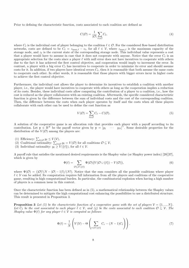
Fig. 5. Case study: Resource Q allocation throughout N tanks.

objective is to determine the cost each player should pay for these communication links according to its contributionto achieve the desired equilibrium. The fair cost that each player should pay is given by the Shapley value.

Let ϕlinks denote the communication cost associated to the undirected graph G (see Figure 1(b)). Therefore, the faircost distribution is given by the Shapley value, i.e.,

L` =Φ(`)∑Nr=1 Φ(r)

ϕlinks, ` ∈ V, (11)

where L` is the fair cost corresponding to the player ` ∈ V. The Shapley value is normalized in (11) since it iscomputed in terms of the error rather than in economical units. These communication links allow sharing, in alocal way, information about the measured levels in order to achieve the first control objective. Notice that this is adecentralized control scheme since each control input is computed by using only partial and local information.

In order to solve the control problem, it is proposed to make a partitioning based on the Shapley value as presentedin Section 4. Therefore, the individual cost associated to each player is the error between the current level and themaximum level of each tank, i.e.,

C` = hmax,` − h`, (12)

where hmax,` denotes the maximum and constant possible level for the `th tank, and hl is the current measured level ofthe `th tank. Once the partitions are determined, a population-dynamics approach is applied to each partition, wherethe fitness function for each strategy is given by the error defined according to Proposition 2, i.e., f` = hmax,` − h`,for all ` ∈ V. It is assumed that this fitness function is always non-negative since physically the current measuredlevel is h` ≤ hmax,`. Notice that, with this fitness function, more resource is assigned to those tanks with lower level.The dynamics for the `th tank are given by

h` = qin,` − qout,`,qout,` = K`h`,

where h` is the current level, qin,` is the inflow, qout,` is the outflow, and K` is a constant factor characterizingthe outflow, for the `th tank. There is a constant available resource given by Q = 30 m3/s. Each inflow qin,` iscontrolled by a valve commanded by a control signal x`, i.e., qin,` = Qx`, with 0 ≤ x` ≤ 1. It is assumed that thereis a local controller at each valve that guarantees the desired flow given by x`. The limited resource establishes a

constraint over all the inflows, i.e.,∑N`=1 qin,` = Q. This equality constraint leads to the condition

∑N`=1Qx` = Q,

and consequently,∑N`=1 x` = 1, then x ∈ ∆. This condition is also satisfied in the partitioned system if the initial

condition of the proportion of agents satisfies∑j∈Pi

1>Nj

i

xji (0) = 1, for the initial topology i ∈ T , due to Proposition

1.

In order to analyze the performance of the closed-loop system composed of the flow-based distribution network andthe population dynamics, three Key Performance Indicators (KPIs) are stated.

• The costs associated to the communication links ϕlinks is taken as a KPI given by

ϕlinks =1

2

∫ tf

t0

1>NAi1N dt, i ∈ T , (13)

for the current topology i ∈ T , where t0 is an initial time and tf a final time.

13

• The error of each tank level with respect to the average levels of the system tanks is also considered as a performanceindicator, i.e.,

ϕerror,` =

∫ tf

t0

(h` −

1

Nh>1N

)dt, ` ∈ V,

where h = [h1 · · · hN ]>. Then, there is a KPI for the whole system in function of the mentioned error levels,i.e.,

ϕerror =

N∑`=1

ϕerror,`.

• The settling time of the system states (level of tanks) with criterion of the 5%, i.e.,

ϕsettling = mint{t : t ≥ t, h ≤ h(t) ≤ h},

where h = 0.95h∗, h = 1.05h∗, with h∗ corresponds to the equilibrium point of the system.

5.1 Results

As a reference to analyze the performance of the proposed control strategy, results for the centralized case are alsopresented. This is equivalent to the case with a topology given by a complete graph (see Figure 6).

Fig. 6. Complete graph given by the grand coalition.

For this example, τ = 2.5 s, and the Shapley value is computed as a function of the error costs in (12). It is importantto mention that the initial condition for each tank level has been established as a random value from the interval[0, 1]. The objectives are: i) maintain all the tank levels at the same maximum value; and ii) determine the fair costsfor the players.

Figure 7 shows the evolution of the tank levels for three different cases (partitions of 2 players, partitions of 3 playersand the grand partition), where it is also shown the gap that determines the settling time. Every τ , the topologyof the system is determined. In Figure 7, it can be also seen that the first objective is met for all the cases. Thesecond objective is achieved by determining the Shapley value as presented in Table 2. Figure 8 shows some differenttopologies obtained based on the Shapley value (see Algorithm 1) at five time instants. In that figure, it can be seenhow topologies vary dynamically with partitions of two and three players.

Figure 9 shows a sensitivity analysis for the evolution of the tank levels for Ns = 10 different scenarios. The onlydifference among these ten scenarios is the vector of initial conditions, which are selected randomly within the interval[0, 2]. First, it is presented the mean of all the tank levels for the scenarios, i.e.,

%(h(wδ)) =1

NsN

Ns∑s=1

N∑i=1

hsi (wδ),

where w = 1, . . . , 2000, are the data used to make the sensitivity analysis, δ = 0.1 s in order to cover the wholesimulation time (i.e., tf = 200 s), and hsi corresponds to the tank i ∈ V in the sth simulation. Then, the standard

14

tank

level

[m]

tank

level

[m]

tank

level

[m]

time [s] time [s] time [s]

(a) (b) (c)

Fig. 7. Evolution of the 13 tank levels for three different cases: (a) partitions of two players, (b) partitions of three players,and (c) partition of N players (full information). Initial condition for each tank level has been determined by a random valuewithin the interval [0, 1].

t = 2.5 s t = 40 s t = 80 s t = 120 s t = 160 s

2P

layer

s3

Pla

yer

s

Fig. 8. Evolution of the graph topologies given by partitions of two and three players (i.e., g = 2, and g = 3), for five differentiterations.

mea

n(h

),σ

[m]

mea

n(h

),σ

[m]

mea

n(h

),σ

[m]

time [s] time [s] time [s]

(a) (b) (c)

Fig. 9. Sensitivity analysis made based on scenarios with random initial conditions with N = 13 tank levels. Mean evolutionof the tank levels and their corresponding standard deviation along the time for three different cases: (a) partitions of twoplayers, (b) partition of three players, and (c) partition of N players (full information).

deviation throughout time is presented to analyze the transitory event for each one of the three cases, partitions of

15

Table 2Fair economical costs for each player determined with the Shapley value.

Player Fair costs according Shapley value

` ∈ V (Φ(`)ϕlinks)/(∑N

r=1 Φ(r))

1

2

3

4

5

6

7

8

9

10

11

12

13

Total

Partitions 2 Players Partitions 3 Players

101.9982 162.7683

103.4772 164.7666

103.0618 175.4056

67.3064 161.5046

69.9416 294.2980

69.7096 146.2820

78.9709 215.1184

123.0623 167.3544

91.6612 290.9280

76.7914 146.8018

99.1411 154.4804

75.6172 170.1767

139.2561 150.1145

1200 2400

two players, three players, and the grand partition. The standard deviation is computed as follows:

σ(wδ) =

√√√√ 1

NsN

Ns∑s=1

N∑i=1

(hsi (wδ)− %(h(wδ))

)2.

It can be seen in Figure 9 that the standard deviation is smaller as there is an evolution of the tank levels. Besides,the standard deviations are reduced more quickly when there are larger partitions. This fact is because when havingbigger partitions, there are more communication exchange among strategies in the population game achieving theclosed-loop system equilibrium in a faster way. The graph sequence presented in Figure 8 varies as the initialconditions are modified because the Shapley value depends on them. However, the sensitivity analysis presented inFigure 9 shows that the system achieves the equilibrium point for all the different initial conditions.

Finally, the comparison of the three cases with the proposed KPI is presented in Table 3. In these results, it can beseen the proper performance of the proposed methodology with respect to the centralized case with full information(partition of N players). Economical costs are reduced significantly, but it implies an increment of the transitoryerrors and settling time of the system states (tank levels).

Table 3Closed-loop system performance for different topologies. Coalitions of two and three players, and with full information.

Players per Communication Error Settling time

partitions g ϕlinks ϕerror ϕsettling

2 players 1200 197.1742 33.23

3 players 2400 58.1723 21.80

N players 15600 20.9294 19.73

5.2 Discussion

In general, game theory models the interaction between rational players. The two different main approaches, thecooperative and the non-cooperative game directions, solve quite different problems. One approach addresses prob-lems in which there is competition whereas the other one is more appropriate to model cooperation. As it has been

16

seen here, it is possible to face engineering applications by implementing both approaches in different but relatedobjectives.

The combination of both approaches demands that the elements within the system take different roles. For instance,in the presented flow-based distribution network, storage nodes represent strategies in the non-cooperative gameapproach. In contrast, storage nodes assume the role of players that demand information by using the communicationnetwork in the cooperative game. This multi-role situation is quite interesting due to the fact that each role is tightlyrelated to each particular control objective, i.e., the optimal resource distribution for the non-cooperative game andboth the fair distribution of costs and proper partitioning for the cooperative game.

It has been shown that the closed-loop system with the non-cooperative approach (i.e., with both the replicator andthe projection dynamics) is stable, performing the partitioning criteria based on cooperative games. This is achievedbased on the assumption that all the partitions, for all the topologies, form a complete graph. Aditionally, whenselecting conveniently the characteristic function of the cooperative game, it is possible to compute the Shapley valueof the whole set of players from the Shapley value of any arbitrary player by following a polynomial-time procedure.Moreover, it has been shown that, by taking advantage of the coalition rationality axiom, it is possible to computethe Shapley value by solving a set of linear equations. This result allows to reduce considerably the computationalburden from an exponential-time procedure to a polynomial one. Besides, due to the fact that the computationcan be reduced, it is also possible to spend time to compute the Shapley value under a distributed structure. Forexample, the comparison of the computational burden in Table 1 shows less computation cost, for the distributedstructure with respect to the traditional Shapley equation and a case involving more than ten players.

6 Conclusions

A control problem involving two objectives associated to competition and cooperation has been presented. In par-ticular, a flow-based distribution network composed of different sub-systems (storage nodes) has been considered.The first objective is associated to an optimal distribution of the available resource, i.e., it is desired to achieve amaximum and equal amount of resource throughout all the sub-systems (storage nodes). To this end, a communica-tion network allows the interaction among different storage nodes, whose communication links have an economicalcost. As a second objective, it is desired to distribute the costs of the communication network throughout the sub-systems, where more influent tanks (with higher power index) must pay less than those with lower influence (withlower power index), i.e., it is desired to assign fair costs for each storage node according to their contributions to theachievement of the first objective. A non-cooperative-game approach is used to solve the former objective, whereasa cooperative-game approach is proposed to solve the latter objective.

Furthermore, for the non-cooperative-game approach, the stability of the closed-loop system is analyzed to guaranteethat the first objective is achieved. On the other hand, regarding the cooperative-game approach that determines thefair distribution of communication costs, an alternative way to compute the Shapley value for the selected specificcharacteristic function has been presented in order to mitigate the computation burden. The proposed approach alsoallows the computation of the Shapley value under distributed structures within reasonable computational timeswith respect to the standard computation.

Moreover, bigger partitions imply more information exchange among the storage nodes, and therefore the resourcedistribution objective is achieved faster. Simulation results have shown that the steady state is achieved faster asthe number of players in the partitions is greater. When having large partitions, the dynamic resource allocation ismade faster due to the fact that there is more available information in the non-cooperative game approach. Never-theless, when having more players making partitions, more communication links are required and this implies highereconomical costs. Furthermore, a smaller overshoot and settling time for the system states (tank levels) are obtainedwhen partitions are larger. Hence, there is a need for balancing economical cost and performance in relation to thecomplexity of the system and the number of players involved in the cooperative game to perform the partitioning.Finally, the sensitivity analysis for the evolution of the system states with arbitrary initial conditions shows that,despite the fact that the partitioning highly depends on the initial conditions of the system, the equilibrium is alwaysachieved.

17

Appendix

Proof of Lemma 1: The storage model dynamics in error coordinates ez` are as follows:

ez` = Q (ex`+ x∗` )−K` (ez` + z∗` ) , for all ` ∈ Vji .

Then, consider the storage function (also Lyapunov function)

L1 =1

2Q

∑i∈T

∑j∈Pi

∑`∈Vj

i

e2z`, (14)

whose derivative is given by

L1 =1

Q

∑i∈T

∑j∈Pi

∑`∈Vj

i

ez` ez` ,

=1

Q

∑i∈T

∑j∈Pi

∑`∈Vj

i

ez`Q (ex`+ x∗` )− ez`K` (ez` + z∗` ) ,

=1

Q

∑i∈T

∑j∈Pi

∑`∈Vj

i

ez`Qex`+ ez`Qx

∗` − e2

z`K` − ez`K`z

∗` ,

=1

Q

∑i∈T

∑j∈Pi

∑`∈Vj

i

ez`Qex`− e2

z`K` + ez` (Qx∗` −K`z

∗` )︸ ︷︷ ︸

z∗`

= 0

,

≤∑i∈T

∑j∈Pi

∑`∈Vj

i

ez`ex`,

=∑i∈T

∑j∈Pi

∑`∈Vj

i

(z` − z∗` ) (x` − x∗` ) ,

=∑i∈T

∑j∈Pi

(zji − zj∗i

)> (xji − xj∗i

).

Then, since(zji − zj∗i

)are the inputs and

(xji − xj∗i

)are the outputs, then L1 ≤

∑i∈T

∑j∈Pi

(zji − zj∗i

)> (xji − xj∗i

)allows to conclude that storage-node dynamics in the flow-based distribution network are passive. �

Proof of Lemma 2: The analysis is made for both replicator and projection dynamics using different storage functions.

Replicator dynamics: consider the entropy function as a storage function (also Lyapunov function)

L2(x) = −∑i∈T

∑j∈Pi

∑`∈Vj

i

xj∗i,` ln

(xji,`

xj∗i,`

), (15)

= −∑i∈T

∑`∈V

xl∗ ln

(x`x`∗

),

which is a valid Lyapunov function since L(x∗) = 0 and L(x) > 0, for all x 6= x∗, fact that is verified by us-ing the Jensen’s inequality (i.e., E(g(x)) ≥ g(E(x)) for any convex function as the logarithm [13]), e.g., L(x) ≥−∑i∈T ln

(∑`∈V

x∗`x`

x∗`

), and due to the fact that ln

(∑`∈V x

∗`x`

x∗`

)= ln (1), it follows that L(x) ≥ 0. Then L(x) > 0,

for all x 6= x∗. Hence,

L2(x) = −∑i∈T

∑j∈Pi

∑`∈Vj

i

xj∗i,`

xji,`xji,`. (16)

18

Replacing dynamics (2) in (16) yields

L2(x) = −∑i∈T

∑j∈Pi

xji∗>(

f ji −1

mji

1Njixji>

f ji

),

= −∑i∈T

∑j∈Pi

(xji∗> − 1

mji

xji∗>1Nj

ixji>)

f ji ,

=∑i∈T

∑j∈Pi

(xji − xji

∗)>f ji .

Projection dynamics: consider the quadratic error as a storage function (also Lyapunov function), i.e.,

L3(x) =1

2

∑i∈T

∑j∈Pi

∑`∈Vj

i

(xji,` − x

j∗i,`

)2

, (17)

where L(x) > 0 for all x 6= x∗, and L(x∗) = 0. Replacing dynamics (3) in the storage function derivative yields

L3(x) =∑i∈T

∑j∈Pi

(xji − xj∗i

)>(f ji −

1

N ji

1Njif ji>1Nj

i

),

=∑i∈T

∑j∈Pi

(xji − xj∗i

)>f ji −

1

N ji

(xji − xj∗i

)>1Nj

if ji>1Nj

i,

=∑i∈T

∑j∈Pi

(xji − xj∗i

)>f ji −

1

N ji

(xji>1Nj

i− xj∗i

>1Nj

i

)f ji>1Nj

i,

=∑i∈T

∑j∈Pi

(xji − xj∗i

)>f ji .

Then, since f ji are the inputs and(xji − xj∗i

)are the outputs, both results show that the replicator and projection

dynamics are lossless. �

Proof of Lemma 3: Consider the arbitrary initial condition for the storage nodes z(0) ∈ RN≥0, the maximum ca-

pacities for the storage nodes zmax ∈ RN≥0, and the costs Ci(0) = zmax,i − zi(0), for all i ∈ V. Now, consider

r0 = arg maxi∈V Ci(0), and `0 = arg mini∈V Ci(0). Then, it is known that according to Remark 3, Φ(r0) > Φ(`0) andthat r0, `0 ∈ V are assigned to the same partition according to the proposed partitioning procedure (Algorithm 1).It follows that, during the interval time τ with the closed loop presented in Figure 3 and according to Remark 2, itis obtained C`0 ≤ zmax,r0 − zr0(τ) ≤ Cr0 , and C`0 ≤ zmax,r0 − zr0(τ) ≤ Cr0 . Then computing r1 = arg maxi∈V Ci(τ),and `1 = arg mini∈V Ci(τ), it is obtained that C`0 ≤ C`1 , and Cr1 ≤ Cr0 .Making the partitioning, it follows that C`0 ≤ C`1 ≤ zmax,`1 − z`1(2τ) ≤ Cr1 ≤ Cr0 , and C`0 ≤ C`1 ≤ zmax,r1 −zr1(2τ) ≤ Cr1 ≤ Cr0 . It is concluded that

mini∈V

Ci(kτ) ≤ zmax,` − z`((k + 1)τ) ≤ maxi∈V

Ci(kτ),

mini∈V

Ci(kτ) ≤ zmax,r − zr((k + 1)τ) ≤ maxi∈V

Ci(kτ),

where r = arg maxi∈V Ci(kτ), and ` = arg mini∈V Ci(kτ). Then[maxi∈V Ci(kτ) − mini∈V Ci(kτ)] → 0 as k → ∞, until maxi∈V Ci(kτ) = mini∈V Ci(kτ). This situation leads tothe equilibrium z∗r = z∗` , for all r, ` ∈ V. Consequently, it is obtained that all fitness functions are the same, then x∗`is achieved for all ` ∈ V. �

Proof of Proposition 1: The invariant-set property is analyzed for both population dynamics.

19

Replicator dynamics: in order to prove that the simplex ∆ is an invariant set, it is shown that the sum of xji for alltopologies i ∈ T and for all partitions j ∈ Pi is null:

∑i∈T

∑j∈Pi

1>Nj

i

xji =∑i∈T

∑j∈Pi

xji>(

f ji −1

mji

1Njixji>

f ji

),

=∑i∈T

∑j∈Pi

(xji>

f ji −1

mji

xji>1Nj

ixji>

f ji

),

=∑i∈T

∑j∈Pi

(xji>

f ji − xji>

f ji

),

= 0.

Projection dynamics: in order to prove that the simplex ∆ is an invariant set, it is shown that the sum of xji for alltopologies i ∈ T and for all partitions j ∈ Pi is null:

∑i∈T

∑j∈Pi

1>Nj

i

xji =∑i∈T

∑j∈Pi

1>Nj

i

(f ji −

1

N ji

1Njif ji>1Nj

i

),

=∑i∈T

∑j∈Pi

1>Nj

i

f ji −1

N ji

1>Nj

i

1Njif ji>1Nj

i.

Notice that 1

Nji

1>Nj

i

1Nji

= 1, then

∑i∈T

∑j∈Pi

1>Nj

i

xji =∑i∈T

∑j∈Pi

1>Nj

i

f ji − f ji>1Nj

i,

= 0.

Both results complete the proof. �

Proof of Proposition 2: Consider the Lyapunov function given by L = L1 + L2 for the replicator dynamics, andL = L1 + L3 for the projection dynamics, where L1, L2 and L3 are the functions presented in (14), (15), and (17),

respectively. According to Lemmas 1 and 2, for both cases L is as follows:

L ≤∑i∈T

∑j∈Pi

(zji − zj∗i

)> (xji − xj∗i

)+∑i∈T

∑j∈Pi

(xji − xj∗i

)>f ji . (18)

Adding and substracting∑i∈T

∑j∈Pi

zjmax,i in (18) yields

L ≤∑i∈T

∑j∈Pi

(−zjmax,i + zji + zjmax,i − zj∗i

)> (xji − xj∗i

)+∑i∈T

∑j∈Pi

(xji − xj∗i

)>f ji ,

=∑i∈T

∑j∈Pi

{(−zjmax,i + zji

)> (xji − xj∗i

)+(zjmax,i − zj∗i

)> (xji − xj∗i

)+ f ji

> (xji − xj∗i

)},

=∑i∈T

∑j∈Pi

{−f ji

> (xji − xj∗i

)+ f j∗i

> (xji − xj∗i

)+ f ji

> (xji − xj∗i

)},

= 0.

Therefore, the equilibrium point (zj∗i ,xj∗i ), for all partitions j ∈ Pi in the topology i ∈ T , is stable. �

20

Acknowledgements

Authors would like to thank COLCIENCIAS (grant 6172) and Agencia de Gestio d’Ajust Universitaris i de RecercaAGAUR (FI 2014) for supporting J. Barreiro-Gomez. Authors also would like to thank the projects DEOCS (Ref.DPI2016-76493-C3-3-R), “Control Predictivo en Red” (Ref. DPI2008-05818) from the Spanish Ministry of Scienceand Education; and the European project FP7-ICT DYMASOS (grant agreement 611281), which have partiallysupported this work.

References

[1] J. Barreiro-Gomez, G. Obando, G. Riano-Briceno, N. Quijano, and C. Ocampo-Martinez. Decentralized control for urban drainagesystems via population dynamics: Bogota case study. In Proceedings of the European Control Conference (ECC), pages 2431–2436,Linz, Austria, 2015.

[2] J. Barreiro-Gomez, C. Ocampo-Martinez, J.M. Maestre, and N. Quijano. Multi-objective model-free control based on populationdynamics and cooperative games. In Proceedings of the IEEE Conference on Decision and Control (CDC), pages 5296–5301, Osaka,Japan, 2015.

[3] J. Barreiro-Gomez, N. Quijano, and C. Ocampo-Martinez. Constrained distributed optimization: A population dynamics approach.Automatica, 69:101–116, 2016.

[4] T. Basar and G. J. Olsder. Dynamic Noncooperative Game Theory. Academic Press, London/New York, 1995.

[5] K. Cai and H. Ishii. Average consensus on arbitrary strongly connected digraphs with time-varying topologies. IEEE Transactionson Automatic Control, 59:1066–1071, 2014.

[6] F. Fele, J. M. Maestre, and E. F. Camacho. Coalitional control: Cooperative game theory and control. IEEE Control Systems,37(1):53–69, 2017.

[7] F. Fele, J. M. Maestre, M. Hashemy, D. Munoz de la Pena, and E. F. Camacho. Coalitional model predictive control of an irrigationcanal. Journal of Process Control, 24:314 – 325, 2014.

[8] M. J. Fox and J. S. Shamma. Population games, stable games, and passivity. Games, 4(4):561–583, 2013.

[9] F. Garin and L. Schenato. A survey on distributed estimation and control applications using linear consensus algorithms. NetworkedControl Systems, 406:75–107, 2010.

[10] R. Gopalakrishnan, J. Marden, and A. Wierman. Characterizing distribution rules for cost sharing games. In Proceeding of the 5thInternational Conference on Network Games, Control and Optimization (NetGCooP), pages 1–4, Paris, France, 2011.

[11] J. Grosso. Economic and Robust Operation of Generalised Flow-based Networks. Doctoral dissertation. Universidad Politecnica deCatalunya. Automatic Control Department, 2015.

[12] J. Hofbauer and W. H. Sandholm. Stable games and their dynamics. Journal of Economic Theory, 144(4):1665–1693, 2009.

[13] J. L. W. V. Jensen. Sur les fonctions convexes et les ingalits entre les valeurs moyennes. Acta Mathematica, 30(1):175–193, 1906.

[14] M. Jilg and O. Stursberg. Optimized distributed control and topology design for hierarchically interconnected systems. In Proceedingsof the 2013 European Control Conference, pages 4340–4346, Zurich, Switzerland, 2013.

[15] M. A. Khan, H. Tembine, and A. V Vasilakos. Evolutionary coalitional games: design and challenges in wireless networks. IEEEWireless Communications, 19(2):50–56, 2012.

[16] S. Li, Y. Zhang, and Q. Zhu. Nash-optimization enhanced distributed model predictive control applied to the shell benchmarkproblem. Information Sciences, 170(2-4):329–349, 2005.

[17] J. M. Maestre and R. R. Negenborn, editors. Distributed Model Predictive Control Made Easy, volume 69 of Intelligent Systems,Control and Automation: Science and Engineering. Springer, 2014.

[18] J.M. Maestre, D. Munoz de la Pena, A. Jimenez Losada, E. Algaba, and E.F. Camacho. A coalitional control scheme with applicationsto cooperative game theory. Optimal Control Applications and Methods, 35:592–608, 2014.

[19] J. Marden and J. Shamma. Game theory and distributed control, volume 4, chapter Handbook of Game Theory with EconomicApplications, pages 861–899. Elsevier, 2015.

[20] F. Muros, J.M. Maestre, E. Algaba, C. Ocampo-Martinez, and E. F. Camacho. An application of the Shapley value to performsystem partitioning. In Proceedings of the American Control Conference (ACC), pages 2143–2148, Chicago, Illinois, 2015.

[21] F. J. Muros Ponce, J. M. Maestre, E. Algaba, T. Alamo, and E. F. Camacho. An iterative design method for coalitional controlnetworks with constraints on the Shapley value. In Proceedings of the 19th IFAC World Congress, pages 1188–1193, Cape Town,South Africa, 2014.

[22] R. B. Myerson. Game Theory. Analysis of Conflict. Hardvard University Press, 1997.

[23] A. Nagurney and D. Zhang. Projected dynamical systems in the formulation, stability analysis, and computation of fixed demandtraffic network equilibria. Transportation Science, 31:147–158, 1997.

[24] J. Nash. Equilibrium points in n-person games. Proceedings of the National Academy of Sciences, 36:48–49, 1950.

[25] A. Nunez, C. Ocampo-Martinez, J.M. Maestre, and B. De Schutter. Time-Varying Scheme for Noncentralized Model PredictiveControl of Large-Scale Systems. Mathematical Problems in Engineering, (v2015):1–17, 2015.

21

[26] G. Obando, A. Pantoja, and N. Quijano. Building Temperature Control based on Population Dynamics. IEEE Transactions onControl Systems Technology, 22(1):404–412, 2014.

[27] R. Olfati-Saber, J.A. Fax, and R.M. Murray. Consensus and cooperation in networked multi-agent systems. Proceedings of theIEEE, 95(1):215–233, 2007.

[28] G. Owen. Game Theory. Academic Press, 1995.

[29] A. Pantoja and N. Quijano. A population dynamics approach for the dispatch of distributed generators. IEEE Transactions onIndustrial Electronics, 58(10):4559–4567, 2011.

[30] A. Pashaie, L. Pavel, and C. J. Damaren. Population dynamics approach for resource allocation problems. In Proceedings of theAmerican Control Conference (ACC), pages 5231–5237, Chicago, IL, USA, 2015.

[31] N. Quijano, C. Ocampo-Martinez, J. Barreiro-Gomez, G. Obando, A. Pantoja, and E. Mojica-Nava. The role of population gamesand evolutionary dynamics in distributed control systems. IEEE Control Systems, 37(1):70–97, 2017.

[32] E. Ramirez-Llanos and N. Quijano. A population dynamics approach for the water distribution problem. International Journal ofControl, 83(9):1947–1964, 2010.

[33] S. Riverso, M. Farina, and G. Ferrari-Trecate. Plug-and-play decentralized model predictive control for linear systems. IEEETransactions on Automatic Control, 58(10):2608–2614, 2013.

[34] N.R. Sandell, P. Varaiya, M. Athans, and M.G. Safonov. Survey of decentralized control methods for large scale systems. IEEETransactions on Automatic Control, 23(2):108–128, 1978.

[35] W. H. Sandholm. Population games and evolutionary dynamics. Cambridge, Mass. MIT Press, 2010.

[36] W. H. Sandholm, E. Dokumaci, and R. Lahkar. The projection dynamic and the replicator dynamic. Games and Economic Behavior,64(2):666–683, 2008.

[37] L.S. Shapley. A value for n-person games. Annals of Mathematics Studies, 28:307–317, 1953.

[38] P. D. Taylor and L. B. Jonker. Evolutionary stable strategies and game dynamics. Mathematical Biosciences, 40(1):145–156, 1978.

[39] H. Tembine, E. Altman, R. El-Azouzi, and Y. Hayel. Evolutionary games in wireless networks. IEEE Transactions on Systems,Man, and Cybernetics, Part B: Cybernetics, 40(3):634–646, 2010.

22