design and modeling of centralized distribution network ... · design and modeling of centralized...
TRANSCRIPT
Design and Modeling of Centralized Distribution Network for the DC House
Project
A Thesis
presented to
the Faculty of California Polytechnic State University,
San Luis Obispo
In Partial Fulfillment
of the Requirements for the Degree
Master of Science in Electrical Engineering
by
Harpreet S. Bassi
June, 2013

ii
© 2013
Harpreet S. Bassi
ALL RIGHTS RESERVED

iii
COMMITTEE MEMBERSHIP
TITLE: Design and Modeling of Centralized Distribution
Network for the DC House Project
AUTHOR: Harpreet S. Bassi
DATE SUBMITTED: June, 2013
COMMITTEE CHAIR: Dr. Taufik, Professor, Electrical Engineering
COMMITTEE MEMBER: Dr. Ali O. Shaban, Professor, Electrical Engineering
COMMITTEE MEMBER: Dr. Tina Smilkstein, Professor, Electrical
Engineering

iv
ABSTRACT
Design and Modeling of Centralized Distribution Network for the DC House Project
Harpreet S. Bassi
This thesis focuses on the design, modeling, simulation, and performance
evaluation of Centralized Distribution Network for the DC House Project. Power System
Computer Aided Design (PSCAD) is used to model a Centralized PV Source, Battery
Bank, and Distribution Network for 25 DC Houses. Design and modeling of each
component in the proposed system are described. For the performance evaluation,
emphasis is on voltage stability and system reliability under different operating
conditions. Results from the simulation demonstrate the feasibility of the proposed
Centralized Distribution Network for the DC House Project to support the houses during
non-generation periods and distribution network voltage stability under different
operating conditions. Cost analysis also shows the feasibility of the proposed system as
compared to commonly used AC distribution network.
Keywords: DC House, Centralized Distribution Network, Solar Power, Boost Converter,
Buck Converter, Maximum Power Point Tracking, Battery Bank, Voltage Stability, AC
distribution network.

v
ACKNOWLEDGMENTS
I would like to begin by thanking my advisor, Dr. Taufik. I am grateful for his
assistance and guidance throughout the graduate program. I would also like to thank rest
of my graduate committee, Dr. Ali O. Shaban, and Dr. Tina Smilkstein.
Foremost, I would like to express my deepest gratitude to my family; especially to
my late brother Sukhvir Bassi. My brother was a person, I looked up too and could
always count on when things weren’t going so well. Without his love and support none of
this would have been possible. Puneetpal Kaur provided emotional and technical support
that can never be repaid. In addition, I would like to say thanks to my friends for their
support, and making college a great experience.
vi
TABLE OF CONTENTS
List of Tables ..................................................................................................................... ix
List of Figures ......................................................................................................................x
Chapter
1. Introduction ..............................................................................................................1
1.1 DC House Project ........................................................................................5
1.2 Thesis Objectives .........................................................................................6
2. Background ..............................................................................................................8
2.1 Motivation ....................................................................................................8
2.2 AC Distribution ............................................................................................8
2.2.1 AC Distribution Infrastructure ............................................................9
2.2.2 Disadvantages of AC Distribution ....................................................10
2.3 DC Distribution ..........................................................................................13
2.3.1 RV DC Distribution ..........................................................................13
2.3.2 400 VDC Distribution in Telco and Data Centers ............................15
2.4 DC House Configurations ..........................................................................17
2.4.1 Individual DC House Configuration .................................................17
2.4.2 Multiple DC Houses Configuration ..................................................22
2.4.3 Centralized Distribution Network for DC Houses ............................23
3. System Design .......................................................................................................24
3.1 PSCAD Software .......................................................................................24
3.2 High Level System Design ........................................................................25
3.3 PV Cell Circuit Model ...............................................................................27
3.3.1 PV module PSCAD Implementation ................................................31
3.4 PV Maximum Power Point Tracking .........................................................34
3.5 Boost Converter Operation ........................................................................38

vii
3.5.1 Boost Converter PSCAD Implementation ........................................43
3.6 Buck Converter Operation .........................................................................45
3.6.1 Buck Converter PSCAD Implementation .........................................49
3.7 Batter Bank ................................................................................................51
3.7.1 Battery Bank PSCAD Implementation .............................................53
3.8 Distribution Network .................................................................................58
4. System Validation ..................................................................................................63
4.1 MPPT and Boost Converter Validation .....................................................63
4.2 Buck Converter Validation ........................................................................74
4.3 Voltage Stability of the Distribution Network. ..........................................76
4.3.1 Full Load. ..........................................................................................78
4.3.2 Varying Load. ...................................................................................82
4.3.3 Varying Number of Houses Operating .............................................84
4.4 PV Charging the Battery and Supplying the Load.....................................87
4.5: Battery Bank Supplying the Load. ............................................................91
4.5.1 Varying Load. ...................................................................................91
4.5.2 Varying Number of Houses Operating .............................................95
4.6 System Cost Analysis. ...............................................................................97
4.6.1 PV Array and MPPT Charge Controller Cost...................................97
4.6.2 Battery Bank Cost. ..........................................................................100
4.6.3 Distribution Cost. ............................................................................105
4.6.4 AC System Cost. .............................................................................106
5. Conclusion and Future Work ...............................................................................109
5.1 Summary and Conclusion ........................................................................109
5.2 Future Work .............................................................................................110
Bibliography ..................................................................................................112
Appendices .....................................................................................................115
Appendix A ..............................................................................................116
Appendix B ..............................................................................................118
Appendix C ..............................................................................................120

viii
Appendix D ..............................................................................................122
Appendix E ..............................................................................................123
Appendix F...............................................................................................125

ix
LIST OF TABLES
Table Page
3-1: Summary of Perturb & Observe Algorithm. ..............................................35
3-2: Comparison of Flooded Lead-Acid and VRLA Battery Types [23]..........52
3-3: ASCR Conductor Specifications Chart. .....................................................61
4-2: PV Output Voltage, Current, and Power with Varying Temperature. .......66
4-3: PV Output Voltage, Current, and Power with Varying Irradiance. ...........68
4-3: PV Output Voltage, Current and Power with Varying Load. ....................70
4-4: Summary of the Boost Converter Voltages and Duty Cycle with
Increasing Load. .........................................................................................72
4-5: Summary of the Buck Converter Voltages and Duty Cycle with Increasing
Load. ..........................................................................................................75
4-6: Efficiency Summary of the Buck and Boost Converters with Increasing
Load. ..........................................................................................................76
4-7: Distribution Network Voltages with 5 to 25 Houses at 500W. .................85
4-8: PV Array Sizing and Cost Calculations. ....................................................98
4-9: Summary of PV Cost for 85% and 75% System Efficiency. .....................99
4-10: MPPT Charge Controller Cost. ................................................................100
4-11: Battery Bank Sizing for 2 Days of Autonomy Storage............................102
4-12: Battery Cost Varied with System Size and Storage Capacity..................103
4-13: Distribution Wiring Cost for a 10 kW System.........................................105
4-14: Distribution Wiring and Boost Converter Cost. ......................................105
4-15: Total DC System Cost. ............................................................................106
4-16: Total AC System cost. .............................................................................107

x
LIST OF FIGURES
Figure Page
1-1: CO2 Emission by Fuel [1] ............................................................................1
1-2: World CO2 Emission by Sector in 2010 [1] ................................................2
1-3: Cumulative Installations of Worldwide PV by the End of 2011 [3] ............3
2-1: Transmission and Distribution Grid Structure within the Power
Industry [6] ................................................................................................10
2-2: Skin Depth of AC Conductor with Increasing Frequency [6] ...................11
2-3: Conversion Stages in an AC System [20] ..................................................12
2-4: 110/120V – 30 Amp RV Wiring Configurations [5] .................................14
2-5: Conventional 480Vac Telco Center Distribution in the United States
[10] .............................................................................................................15
2-6: Proposed Facility-level 400V DC Power Distribution [10] .......................16
2-7: Comparison of Distribution Systems Efficiencies as a Function of
Load [10] ....................................................................................................17
2-8: Single DC house Configuration [20] .........................................................18
2-9: DC Light Bulb at Full Load from 48 VDC Input [4] .................................20
2-10: Multiple Input Single Output DC-DC Converter Board [16] ....................21
2-11: Multiple DC Houses Configuration [20] ...................................................22
2-12: Proposed Centralized Distribution Network for DC Houses [20] .............23
3-1: Basic Block Diagram of Proposed Design.................................................25
3-2: Detailed Block Diagram of the Proposed System Design .........................27
3-3: PV Cell Equivalent Circuit [28] .................................................................28
3-4: The I-V characteristics of a PV cell [21] ...................................................29
3-5: PV Module Components available in PSCAD ..........................................31
3-6: PV Cell Default Parameters .......................................................................32
3-7: PV Module and PV Array Parameters .......................................................33

xi
3-8: PV Module I-V and Power Characteristics ................................................33
3-9: PSCAD MPPT Component (left), and Parameters (right) .........................34
3-10: Incremental Conductance Based Algorithm MPPT [30] ...........................37
3-11: The Controller used to drive the Boost Converter Switch for MPPT ........38
3-12: Boost Converter Block Diagram [32] ........................................................39
3-13: Conduction Modes of DC-DC Converters [32] .........................................39
3-14: Boost Converter CCM Switch ON State [32] ............................................40
3-15: Boost Converter CCM Switch OFF State [32] ..........................................41
3-16: Boost Converter Inductor, Switch and Diode Current [32] .......................42
3-17: Boost Converter connected to the PV Array in PSCAD ............................43
3-18: Buck Converter Block Diagram [32] .........................................................45
3-19: Buck Converter CCM Switch ON State [32] .............................................46
3-20: Buck Converter CCM Switch OFF State [32] ...........................................47
3-21: Buck Converter CCM Waveforms [34] .....................................................48
3-22: Buck Converter Cascaded with Boost Converter in PSCAD ....................49
3-23: Buck Converter Switch Controller for Regulating Output Voltage at
48V .............................................................................................................50
3-25: Cell Discharge Characteristics of Four Battery Types ..............................51
3-26: Battery Equivalent Circuit Diagram [18] ...................................................53
3-27: Battery Custom Component in available in PSCAD .................................54
3-28: Lead-Acid Battery Parameters ...................................................................55
3-29: Complete Battery Bank Design .................................................................57
3-30: Boost Converter (top) and Controller (bottom) within the Sub-Module
Battery Cascaded .......................................................................................57
3-31: Distribution Network Design for 25 DC Houses .......................................58
3-32: Magnified view of Feeder C Supplying Power to 5 DC Houses ...............59
3-33: DC Equivalent Circuit Diagram [8] ...........................................................60
3-34: Boost Converter (top), and its Switch Controller (bottom) used in
Distribution Network .................................................................................62
4-1: Complete System Design Implemented in PSCAD ...................................64
xii
4-2: PV Module I-V Characteristic with Varying Solar Radiation (left) and
Temperature (right)
[35] .............................................................................................................65
........................................................................................................................
4-3: PV Array output Voltage (top), Current (middle), and Power (bottom)
with Varying Temperature .........................................................................66
4-4: PV Array output Voltage (top), Current (middle), and Power (bottom)
with Varying Solar Irradiance ....................................................................68
4-5: PV Array Voltage Operating Point as the Load Increases .........................69
4-6: PV Array operating Voltage (top), Current (middle), and Power (bottom)
with Varying Load .....................................................................................70
4-7: Boost Converter Input and Output Voltages with increasing Load ...........72
4-8: Boost Converter Inductor Current (top) and Magnified View of Inductor
Current at Full Load (bottom) ....................................................................73
4-9: Buck Converter Input and Output Voltages with increasing Load ............74
4-10: PV Output Power (green) and Buck Converter Output Power (blue) with
Varying Load .............................................................................................75
4-11: Centralized Distribution Network Design for 25 DC Houses ...................77
4-12: Voltages at Five locations in the Distribution Network at Full Load ........78
4-13: Current at Five Locations in the Distribution Network at Full Load .........80
4-14: Power in the main DC Distribution Cable (Top) and Power delivered to 2
individual Houses (bottom)........................................................................81
4-15: Voltage Measurements at Five Locations as load is incremented from
100W to 500W in steps of 50W .................................................................82
4-16: Current Measurements at Five Locations as load is incremented from
100W to 500W in steps of 50W .................................................................83
4-17: Power Measurements at Five Locations as load is incremented from 100W
to 500W in steps of 50W ...........................................................................84
4-18: Voltage Measurements at Five Locations as Number of Houses is
incremented ................................................................................................85

xiii
4-19: Current Measurements at Five Locations as Number of Houses is
incremented ................................................................................................86
4-20: Power Measurements at Five Locations as Number of Houses is
incremented ................................................................................................86
4-21: Battery Storage during Peak Sun Hours (dark yellow) and Battery
Supplying Load (green) .............................................................................87
4-22: Power Supplied to the Battery from PV Array ..........................................88
4-23: Battery Current (blue) and Voltage (green) ...............................................88
4-24: Voltage Measurements of the Distribution Network at Five Locations
While the Battery Bank is being charged ..................................................89
4-25: Current Measurements of the Distribution Network at Five Locations
While the Battery Bank is being charged ..................................................90
4-26: Power Measurements of the Distribution Network at Five Locations While
the Battery Bank is being charged .............................................................90
4-27: Voltage Measurements of Distribution Network at Five Locations as Load
is increased from 100W to 500W in steps of 50W (Powered from Battery)
....................................................................................................................92
4-28: Current Measurements of Distribution Network at Five Locations as Load
is increased from 100W to 500W in steps of 50W (Powered from
Battery) ......................................................................................................93
4-29: Power Measurements of Distribution Network at Five Locations as Load
is increased from 100W to 500W in steps of 50W (Powered from
Battery) ......................................................................................................94
4-30: Battery Bank State of Charge (SOC) .........................................................94
4-31: Voltage Measurements of Distribution Network at Five Locations as
number of houses is incremented (Powered from Battery) .......................95
4-32: Current Measurements of Distribution Network at Five Locations as
number of houses is incremented (Powered from Battery) .......................96
4-33: Power Measurements of Distribution Network at Five Locations as
number of houses is incremented (Powered from Battery) .......................96
xiv
4-34: Jakarta Indonesia Monthly Insolation [36] ................................................97
4-35: DC Distribution PV Cost with 85% and 75% Efficiency ..........................99
4-36: Battery Bank Cost with Increasing System Size and Storage Capacity ..104
4-37: DC System Cost at 85% Efficiency and AC System 75% Efficiency .....108
1
CHAPTER 1
Introduction
More than 80% of world’s energy supply comes from fossil fuel sources like
petroleum, coal, and natural gas. Fossil fuels are nonrenewable energy sources since they
take millions of years to form. When used, fossil fuels release carbon into the atmosphere
which contributes to the greenhouse gases. Global CO2 emissions are rising every year
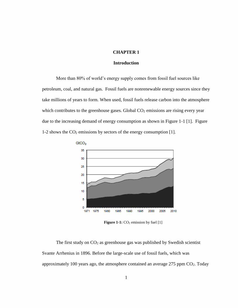
due to the increasing demand of energy consumption as shown in Figure 1-1 [1]. Figure
1-2 shows the CO2 emissions by sectors of the energy consumption [1].
Figure 1-1: CO2 emission by fuel [1]
The first study on CO2 as greenhouse gas was published by Swedish scientist
Svante Arrhenius in 1896. Before the large-scale use of fossil fuels, which was
approximately 100 years ago, the atmosphere contained an average 275 ppm CO2. Today

2
the estimate is 380 ppm CO2 in the atmosphere which is a direct result of the combustion
of fossil fuels. After 100 years of burning fossil fuels, the earth’s average surface
temperature has risen from 57°F to 58.3°F [2]. This is a small change in temperature, but
potentially a large difference in climate which has led to glaciers melting and sea levels
rising. If we continue to use fossil fuels until they run dry, the CO2 concentration is
expected to increase to about 550 ppm. The Intergovernmental Panel on Climate Change
(IPCC) suggests that the average surface temperature will likely rise another 2.0 to 11.5
°F [2].
Figure 1-2: World CO2 emission by sector in 2010 [1]
Global warming issue has made renewable sources of energy more attractive.
Renewable energy is derived from natural processes (e.g. sunlight and wind) that are
replenished at faster rate than they are consumed. Solar, wind, geothermal, hydro and
some forms of biomass are common sources of renewable energy. Solar and wind have
grown the most popular over the past decade. Global wind power capacity was 238
3
(GW) at the end of 2011, up from just 18 GW at the end of 2000. The advancements in
electronics and renewable energy have enabled us to produce energy out of resources
which was impossible 50 years ago. Renewable energy provides secure reliable power
with economic productivity and with little to no environmental impact.
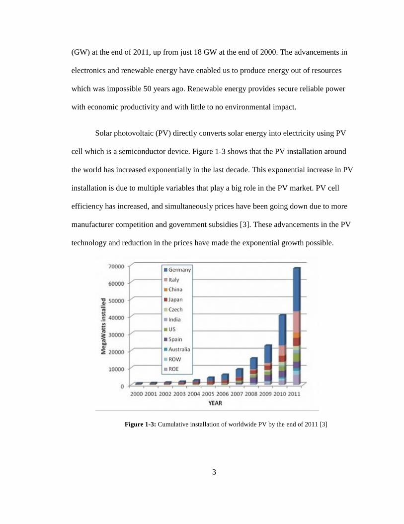
Solar photovoltaic (PV) directly converts solar energy into electricity using PV
cell which is a semiconductor device. Figure 1-3 shows that the PV installation around
the world has increased exponentially in the last decade. This exponential increase in PV
installation is due to multiple variables that play a big role in the PV market. PV cell
efficiency has increased, and simultaneously prices have been going down due to more
manufacturer competition and government subsidies [3]. These advancements in the PV
technology and reduction in the prices have made the exponential growth possible.
Figure 1-3: Cumulative installation of worldwide PV by the end of 2011 [3]

4
Renewable sources of energy also give us the chance to provide energy to
rural areas mainly in under-developed countries which are not likely to be connected to
electric grid. Still today there are about 1.3 billion people around the world who do not
have access to electricity. About 587 million of this population lives in Africa,
approximately 675 million in Asia, and 55 million in Eastern Europe/Eurasia [4].
Generally this population lives in rural areas which are farther away from the urban
electric grid, thus connecting them to an electric grid is not economically viable. The
capital required to build high voltage transmission system for longer distances is very
expensive. According to Edison Electric Institute (EEI), from 2004-2008, United States
invested $4.6M/GW/year, New Zealand invested $ 22.M/GW/year, and the Netherlands
invested $12.0M/GW/year in high voltage transmission [4]. The cost for lower than
230kV will be more for longer distance due to higher resistive losses (I2R) in the grid.
This is because as the transmission voltage is lowered, the resulting current increases
proportionally and the losses in the system increase accordingly.
People who live in rural villages in underdeveloped countries are mostly poor and
are deprived of most basics of human rights, and of economic opportunities to improve
their standard of living without access to electricity. Undoubtedly rural electrification
programs face major obstacles. Utility companies need to have high initial capital along
with high operation costs because of the low population densities in rural areas.
Therefore, it does not create a business advantage to invest on an expensive grid
infrastructure to provide electricity to these people especially since their consumption
will be very low (mostly for lighting). Moreover, building infrastructure for these areas

5
may often create conflicts with the local communities, and farmers due to rights of way
for the construction and maintenance of electricity lines.
Renewable energy is an abundant source of energy which could be used to
provide electricity for those unfortunate people in rural areas with no access to electricity.
The good news is that many of these rural areas happen to be in locations where
renewable energy sources are abundant. For example, majority of this poor population
live within plus or minus 30 degrees of latitude around the world.
1.1 DC House Project
Local electrical network for the unfortunates seems to be a feasible option
available through renewable sources of energy. The DC house project initiated at Cal
Poly is an extension to that idea along with its futuristic benefits. DC house is a project
for the unfortunates. It aims to deliver the most basic electric needs of the modern world
to those in need by utilizing renewable energy sources. The DC house, as the name
implies, operates fully on Direct Current.
Over the century scientific and economic developments have led to expansion of
the electric grid around the world. But as mentioned earlier, still today, after 150 years of
early inventions of electricity, there are approximately 1.3 billion people around the
world who do not have access to electricity. Financial disadvantages and remote locations
of these populations are the two main reasons for their governments not to have the
incentive to connect them to their nations’ grids. The DC house project aims to address
6
these problems and is divided into three phases. Phase 1, which was completed in June
2011, focused on the single DC house development as the basic unit. It included designs
of generator sources such as: Hydro-power generator, a photovoltaic power generator, a
human-powered generator and a wind-powered generator. Phase 1 also included the
designs for multiple-input DC-DC converter, system level design of DC house (DC level
and loads.)
Phase 2 of the project was concluded in June 2012. This phase looked at the
optimization, protection, and implementation of single DC house. Several important
milestones were completed during this phase such as a temporary DC house model at Cal
Poly, DC Lightbulb, publications and presentations of DC house.
Now the project is in Phase 3, which will conclude in June 2013. Phase 3 of the
project is focusing on a centralized DC System, where centralized PV panels are used to
distribute power to a larger village rather than strictly to an individual house.
1.2 Thesis Objective
This thesis falls under the third phase of the DC House project which focuses on
the design, modeling, simulation, and performance evaluation of the centralized
distribution network for the DC House. Power System Computer Aided Design (PSCAD)
is used to simulate the network. This network would include standalone solar PV source
working with Maximum Power Point Tracker (MPPT) to maximize the power production
under different weather conditions. The feasibility, operation, and performance of the

7
DC distribution system are the main goals of the study. Additionally as part of the study,
the implementation of the PV sources with MPPT will consider various conditions that
will affect the power generation and voltage stability in the local DC grid. Load flow
analysis for as many as 25 houses of 500W and their different layouts will be modeled
and analyzed. Backup batteries to provide stability to the grid and backup power during
night and non-power generating conditions will also be studied and considered.

8
CHAPTER 2
Background
2.1: Motivation
The DC house project is a solution to challenges of rural electrification. It will
provide self-sustaining DC power through various forms of renewable energy such as
photovoltaic, hydropower, wind, and human-powered generation. The generated power is
used to provide the most basic living necessities such as room lighting, electric stove for
cooking, space heating, cooling and refrigeration. This renewable form of energy will
replace liquid fuel, gas, biomass or animal waste, which currently help sustain the daily
energy necessities of rural areas in poor nations. This chapter will discuss the commonly
used AC distribution system and the advantages of choosing DC distribution for the DC
house project.
2.2: AC Distribution
In the 1880s, Tesla and Edison went head to head with the “War of Currents” as it
is called [18]. The biggest challenge was to set up an electrical-grid network that would
send power over long distance with minimal losses. This required voltage step-up at the
generation side and step-down on the distribution side. Westinghouse’s invention of the
transformer made it possible for voltage to step-up and step-down in the alternating
current, thus making it the stronger candidate out of the two. Tesla won his battle for
9
alternating current by proving it was the better choice at that time given all the electric
equipment capabilities. This victory paved the way for the AC infrastructure to build over
the past century.
2.2.1: AC Distribution Infrastructure
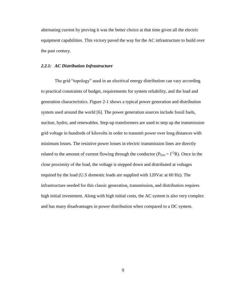
The grid “topology” used in an electrical energy distribution can vary according
to practical constraints of budget, requirements for system reliability, and the load and
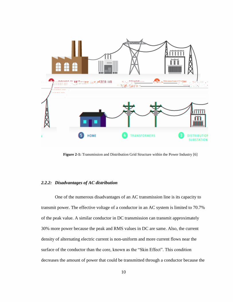
generation characteristics. Figure 2-1 shows a typical power generation and distribution
system used around the world [6]. The power generation sources include fossil fuels,
nuclear, hydro, and renewables. Step-up transformers are used to step up the transmission
grid voltage in hundreds of kilovolts in order to transmit power over long distances with
minimum losses. The resistive power losses in electric transmission lines are directly
related to the amount of current flowing through the conductor (Ploss = I^2R). Once in the
close proximity of the load, the voltage is stepped down and distributed at voltages
required by the load (U.S domestic loads are supplied with 120Vac at 60 Hz). The
infrastructure needed for this classic generation, transmission, and distribution requires
high initial investment. Along with high initial costs, the AC system is also very complex
and has many disadvantages in power distribution when compared to a DC system.
10
Figure 2-1: Transmission and Distribution Grid Structure within the Power Industry [6]
2.2.2: Disadvantages of AC distribution
One of the numerous disadvantages of an AC transmission line is its capacity to
transmit power. The effective voltage of a conductor in an AC system is limited to 70.7%
of the peak value. A similar conductor in DC transmission can transmit approximately
30% more power because the peak and RMS values in DC are same. Also, the current
density of alternating electric current is non-uniform and more current flows near the
surface of the conductor than the core, known as the “Skin Effect”. This condition
decreases the amount of power that could be transmitted through a conductor because the

11
middle portion of the conductor is not being used. As shown in Figure 2-2, the current
density for a DC conductor is uniform throughout, which is not true in AC conductor [6].
In an AC conductor, skin depth decreases as the frequency of current increases, thus
current only flows mainly near the surface of the conductor [6].
Figure 2-2: Skin depth decreases with increasing frequency [6]
The Power Factor of the AC system is another variable that affects AC power
transmission. The reactance of AC transmission lines lowers its Power Factor which
leads to reactive power being drawn out of the generator, and subsequently less real
power is delivered to the load. Another issue of an AC system is its frequency, which is
required to be at 60 Hz for a stable system. An inaccurate frequency control does not
allow efficient flow of power from multiple generators into the grid network. Another
phenomenon in AC transmission is the Corona Discharge Effect in which electrical

12
breakdown is caused by ionization of surrounding air of conductors at voltage amounts
greater than that of the critical breakdown voltage [7].
Many of the domestic loads such as home appliance, electronics, and
entertainment systems require DC power for their operation. The incoming AC from the
power outlet has to be converted to DC in order for these loads to work. This AC to DC
power conversion introduces power losses into the system. Figure 2-3 shows the
conversion stages which are required in an AC system for the DC loads [20].
Additionally, in case of renewable sources, which (generate DC power), the current AC
system requires two conversion stages before power could be delivered to the load.
Figure 2-3: Conversion stages in an AC system [20]
A DC distribution system would eliminate the AC to DC conversion by more
efficient DC-DC conversions. Another benefit of a DC system is that it is less costly
since components are rated at lower voltages. Largely the DC distribution system is less
complex, more efficient and consumes less space. However, AC system was preferred

13
over DC system for the past century because DC did not have the capability to step-up or
step-down voltage without the power electronic technologies. The power electronic
industry has since developed highly reliable and well-performing technologies capable of
these tasks, and DC distribution is now considered as an optimal solution to improve
distribution efficiency.
2.3: DC Distribution
The idea of incorporating one or multiple renewable energy sources to support the
DC system is unique. DC system features lack of frequency stability, reactive power
issues, skin effect, and conversion losses compared to AC power system. Using direct
current to distribute power is not a new concept. As mentioned before, Edison was
promoting DC distribution network during the “War of Currents” era in 1890’s. Also,
RV, Telco and Data centers, aircraft, spacecraft, and ship already used DC distribution
[11].
2.3.1: RV DC Distribution
First example of an existing small DC power distribution system in use is an RV’s
electrical system, as illustrated in Figure 2.4 [5]. The RV’s motor drives an alternator that
produces AC voltage, which is rectified to 12-volt DC to charge the on-board batteries
and supply power to the DC appliances. This 12-volt DC distribution has its own fuses,
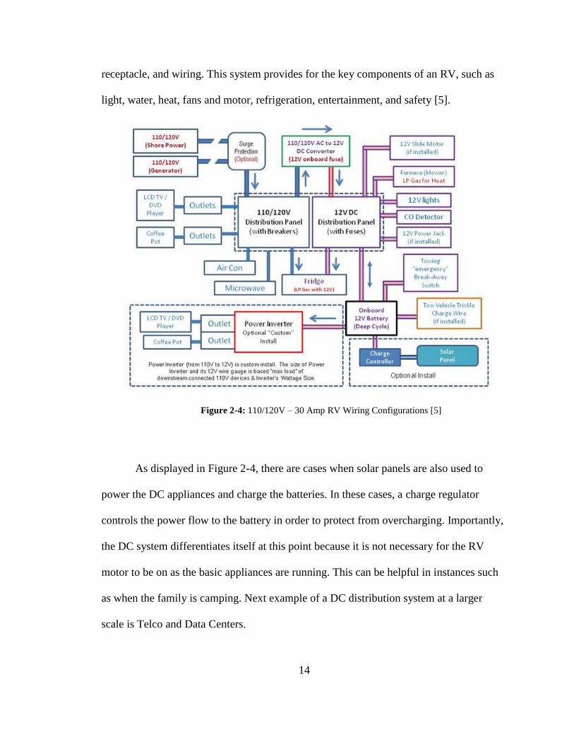
14
receptacle, and wiring. This system provides for the key components of an RV, such as
light, water, heat, fans and motor, refrigeration, entertainment, and safety [5].
Figure 2-4: 110/120V – 30 Amp RV Wiring Configurations [5]
As displayed in Figure 2-4, there are cases when solar panels are also used to
power the DC appliances and charge the batteries. In these cases, a charge regulator
controls the power flow to the battery in order to protect from overcharging. Importantly,
the DC system differentiates itself at this point because it is not necessary for the RV
motor to be on as the basic appliances are running. This can be helpful in instances such
as when the family is camping. Next example of a DC distribution system at a larger
scale is Telco and Data Centers.
15
2.3.2: 400 VDC Distribution in Telco and Data Centers
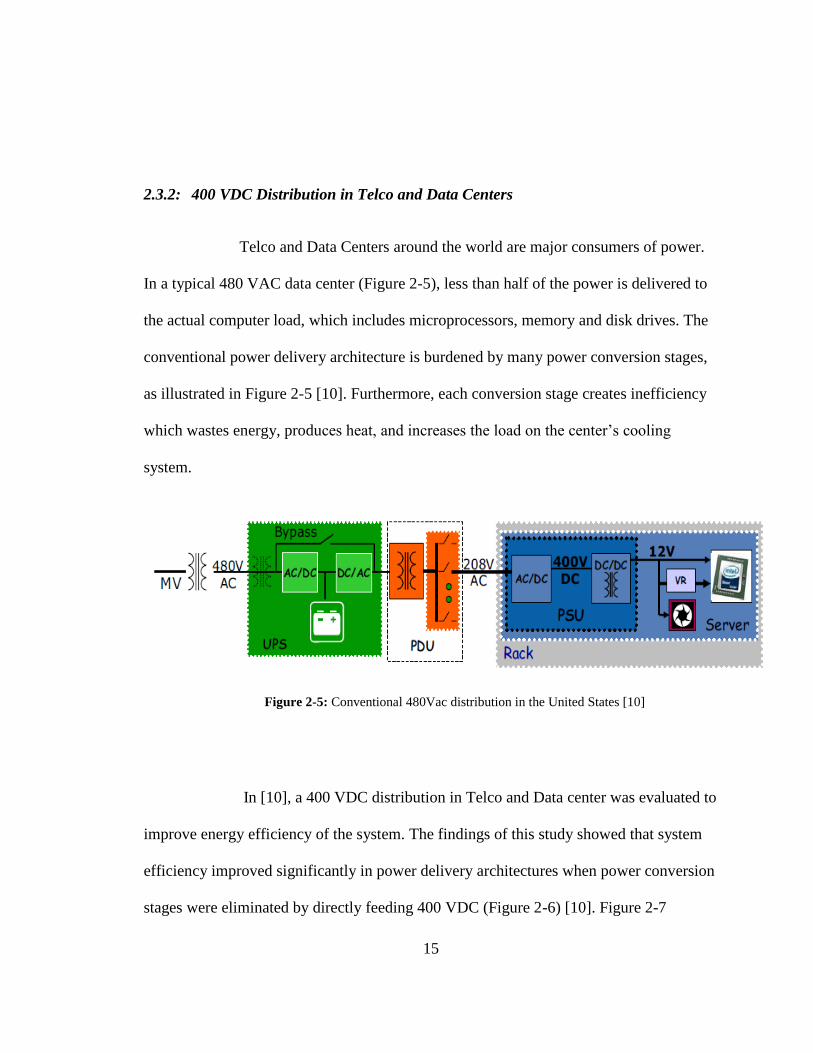
Telco and Data Centers around the world are major consumers of power.
In a typical 480 VAC data center (Figure 2-5), less than half of the power is delivered to
the actual computer load, which includes microprocessors, memory and disk drives. The
conventional power delivery architecture is burdened by many power conversion stages,
as illustrated in Figure 2-5 [10]. Furthermore, each conversion stage creates inefficiency
which wastes energy, produces heat, and increases the load on the center’s cooling
system.
Figure 2-5: Conventional 480Vac distribution in the United States [10]
In [10], a 400 VDC distribution in Telco and Data center was evaluated to
improve energy efficiency of the system. The findings of this study showed that system
efficiency improved significantly in power delivery architectures when power conversion
stages were eliminated by directly feeding 400 VDC (Figure 2-6) [10]. Figure 2-7

16
displays the efficiency plots of power distribution architectures studied in [10] for the
Telco and Data Centers. This study concluded that the two electrical architectures, 400
VDC and 48 VDC, yield the highest efficiency because the conversion stages are
eliminated.
Figure 2-6: Proposed Facility-level 400V DC power distribution [10]
Figure 2-7: Comparison of calculated efficiencies as a function of load [10]

17
2.4: DC House Configurations
There are three different configurations of DC house: Individual DC house,
Multiple DC Houses, and Centralized DC System. These configurations are based on
multiple factors, such as the local population and the spread of the houses. The following
sections discuss these configurations and their processes in further detail.
2.4.1: Individual DC House Configuration
In the Individual DC house configuration, a single DC house operates in islanding
mode, as illustrated in Figure 2-8 [20]. This type of configuration is suitable for villages
with widely disperse population and it can have one or multiple renewable sources
generating DC power. In order to have regulated input into the Multiple Inputs DC-DC
converter (MISO), the renewable sources are followed by the DC-DC converter. This
MISO conversion translates to a single DC bus voltage at 48V which is used to power the
house and charge the battery bank for the night-time use. The completed DC house
projects under this configuration are discussed in the next section.

18
Figure 2-8: Single DC house Configuration [20]
In [14] a bicycle power generator was designed and implemented. The goal was to
have a cost effective human-powered DC generator which could be used in times when
other renewable sources would not be generating power. A car’s alternator, with modified
internal wiring, was attached to the bike’s back tire in order to convert the mechanical
energy into electrical energy. As Figure 2-8 illustrates, this electrical energy then could
be used to provide power straight to the DC house or charge the batteries. The findings of
the study showed that the alternator’s efficiency to convert mechanical energy to
electrical energy is highly dependent on its RPM in conjunction with its internal
resistance. At around 1800 RPM, the alternator’s efficiency was close to 35%. It was also

19
concluded that there is plenty of room for improvements in the lower RPM efficiency.
Other projects focused on additional renewable sources such as wind power [18] and
hydro-electric [19].
In [8] the main DC bus voltage feeding to the house was analyzed for the highest
efficiency. The goal of the project was to determine the adequate DC bus voltage that
would generate the highest system efficiency. It accounted for variables such as mesh and
radial distribution systems, wire size, different loads, and 500W maximum power input.
Subsequently, it was concluded that 48V bus would give the best results in efficiency and
cost of the components [8].
In [9] research was conducted on available DC loads that can be used in the DC
house. A system was designed, modeled, and characterized in steady state using Simulink
toolbox in MATLAB. The selection strategy for the loads were mainly based on fulfilling
the basic humanitarian needs of daily life such as lighting, cooking appliances, and food
storage. Further detailed study was conducted on the individual loads to determine the
best available option in the market, given the capabilities and limitation of DC house. For
example, two types of compressors were studied for the refrigerator load. It was
determined a conventional compressor would not be a good choice of load for the DC
house because it typically requires large amount of start-up current which would exceed
the capabilities of the source given that most of the renewable sources are constant
current source. An alternative swing-compressor available in the market was determined
a better fit because it requires a low startup current. Based on these findings, a
refrigerator available in the market was selected and further studied by creating a model

20
in Simulink based on the characteristics given in the datasheet. To maximize efficiency,
and simultaneously reduce the cost of the system, different circuit configurations were
studied to connect the loads within the DC house while varying the feeder bus voltages
and size of wire used for the circuit [9].
In [4] an economical and energy-efficient DC light bulb was designed and
implemented. This DC Light Bulb was to operate at input voltage ranging from 24 VDC
to 72 VDC as shown in Figure 2-9. Test in the lab showed the DC light bulb is capable of
producing illumination intensities equivalent to a standard 100W A19 incandescent light
bulb at one-tenth the total power consumption. This study demonstrated the feasibility of
the DC Light Bulb in terms of overall efficiency, line regulation, load regulation, power
consumption, total lumens, and thermal profile.
Figure 2-9: Fully DC Light bulb at full load from 48 VDC input [4]
21
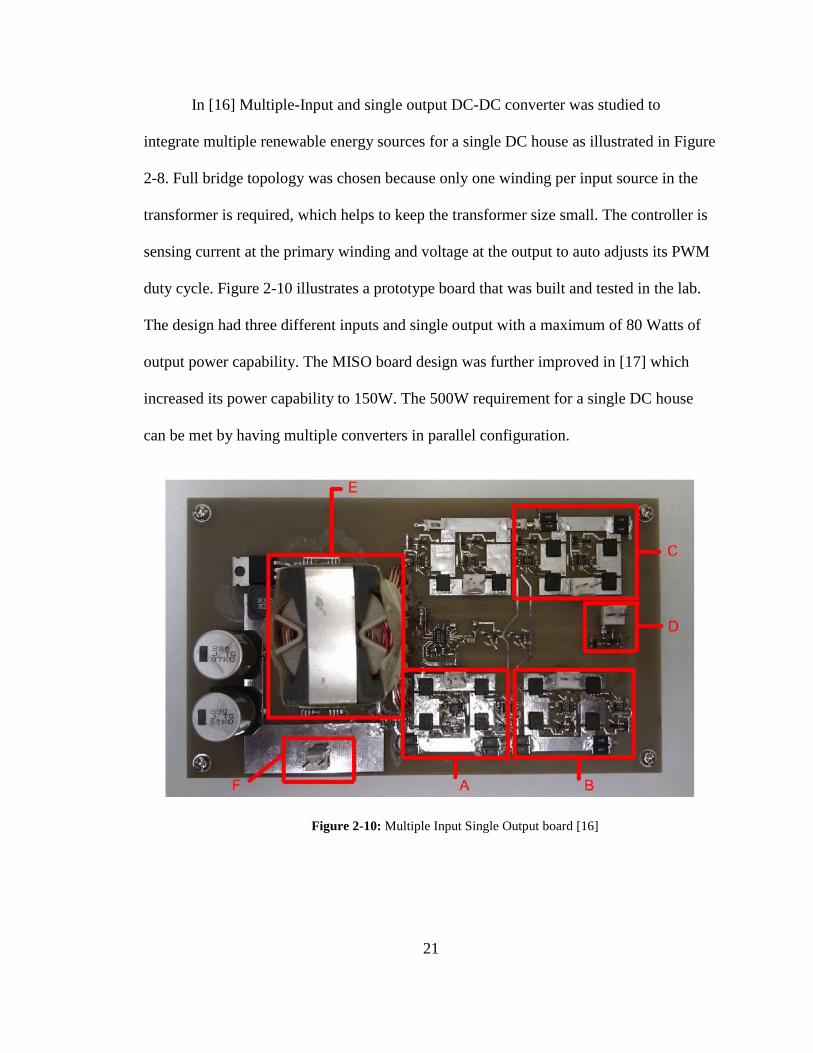
In [16] Multiple-Input and single output DC-DC converter was studied to
integrate multiple renewable energy sources for a single DC house as illustrated in Figure
2-8. Full bridge topology was chosen because only one winding per input source in the
transformer is required, which helps to keep the transformer size small. The controller is
sensing current at the primary winding and voltage at the output to auto adjusts its PWM
duty cycle. Figure 2-10 illustrates a prototype board that was built and tested in the lab.
The design had three different inputs and single output with a maximum of 80 Watts of
output power capability. The MISO board design was further improved in [17] which
increased its power capability to 150W. The 500W requirement for a single DC house
can be met by having multiple converters in parallel configuration.
Figure 2-10: Multiple Input Single Output board [16]
22
2.4.2: Multiple DC Houses Configuration
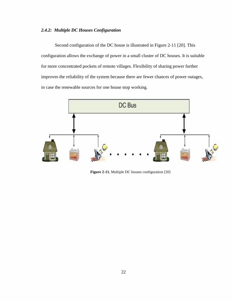
Second configuration of the DC house is illustrated in Figure 2-11 [20]. This
configuration allows the exchange of power in a small cluster of DC houses. It is suitable
for more concentrated pockets of remote villages. Flexibility of sharing power further
improves the reliability of the system because there are fewer chances of power outages,
in case the renewable sources for one house stop working.
Figure 2-11. Multiple DC houses configuration [20]
23
2.4.3: Centralized Distribution Network for DC Houses
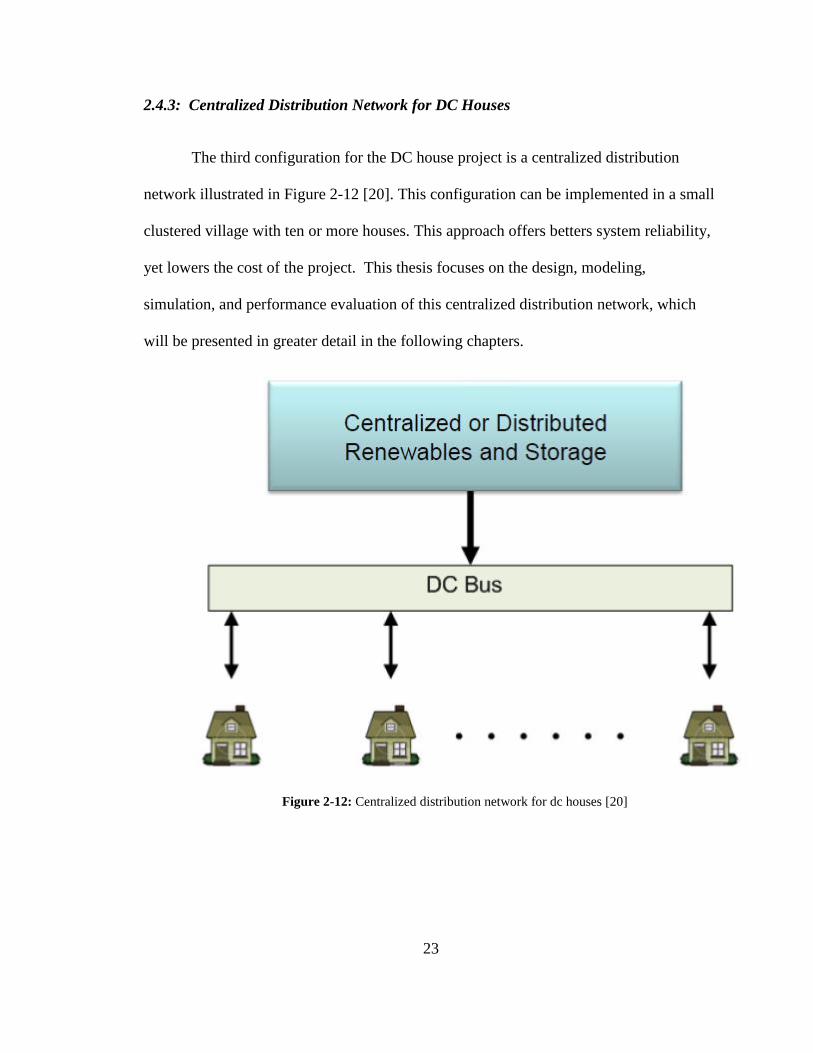
The third configuration for the DC house project is a centralized distribution
network illustrated in Figure 2-12 [20]. This configuration can be implemented in a small
clustered village with ten or more houses. This approach offers betters system reliability,
yet lowers the cost of the project. This thesis focuses on the design, modeling,
simulation, and performance evaluation of this centralized distribution network, which
will be presented in greater detail in the following chapters.
Figure 2-12: Centralized distribution network for dc houses [20]
24
CHAPTER 3
System Design
3.1: PSCAD Software
The electric grid has remained unaffected since the 20th century’s
technological advancements. But the recent integration of power electronics and
communication devices into the grid is changing this hundred-year-old infrastructure into
a smarter grid. In the so-called “Smart Grid” infrastructure, energy would be generated,
distributed and used more efficiently. However these new power electronic and
communication devices pose problems for most of the existing power system design
software because the scope of their capabilities to simulate behavior of these new
electronic devices is very limited. These simulation challenges are resolved by using
Power System Computer Aided Design (PSCAD) software package developed by
Manitoba HVDC Research Center. The PSCAD simulation tool can duplicate the
response of power electronic devices in time steps ranging from nanoseconds to seconds
[31]. Other power electronic simulation software packages, such as PSpice, are general
purpose analog and mixed-signal simulator used to verify circuit design and to predict
circuit behavior. Whereas, PSCAD is specifically targeted to simulate power systems and
power electronic circuits [31]. Since the simulation model of the Centralized DC House
Distribution Network will have power systems and power electronic components,

25
PSCAD was chosen as the best available option to simulate the behavior of the
centralized DC house distribution network.
3.2: High Level System Design
The centralized DC House distribution network is a solution to provide electricity
to rural and isolated populations with low cost and high system reliability. As mentioned
in the previous chapter, multiple renewable sources can be used to generate power for the
DC house as well. But this study only focuses on solar power generation as the source of
power for the centralized DC House distribution network. Figure 3-1 illustrates the
fundamental block diagram of the proposed design for the centralized DC House
distribution network.
Figure 3-1: Basic block diagram of proposed design

26
The power generated by PV array varies according to the solar irradiance,
temperature, and load demand. These three variables control the voltage operating point
of the PV array, which determines the amount of power generated. A Maximum Power
Point Tracking device is used to keep the voltage operating point of the PV array around
the knee of the I-V curve, which extracts maximum amount of power. Battery bank stores
the excess power generated during the peak sunlight hours, and supplies it to the load at
night or in cloudy weather conditions.
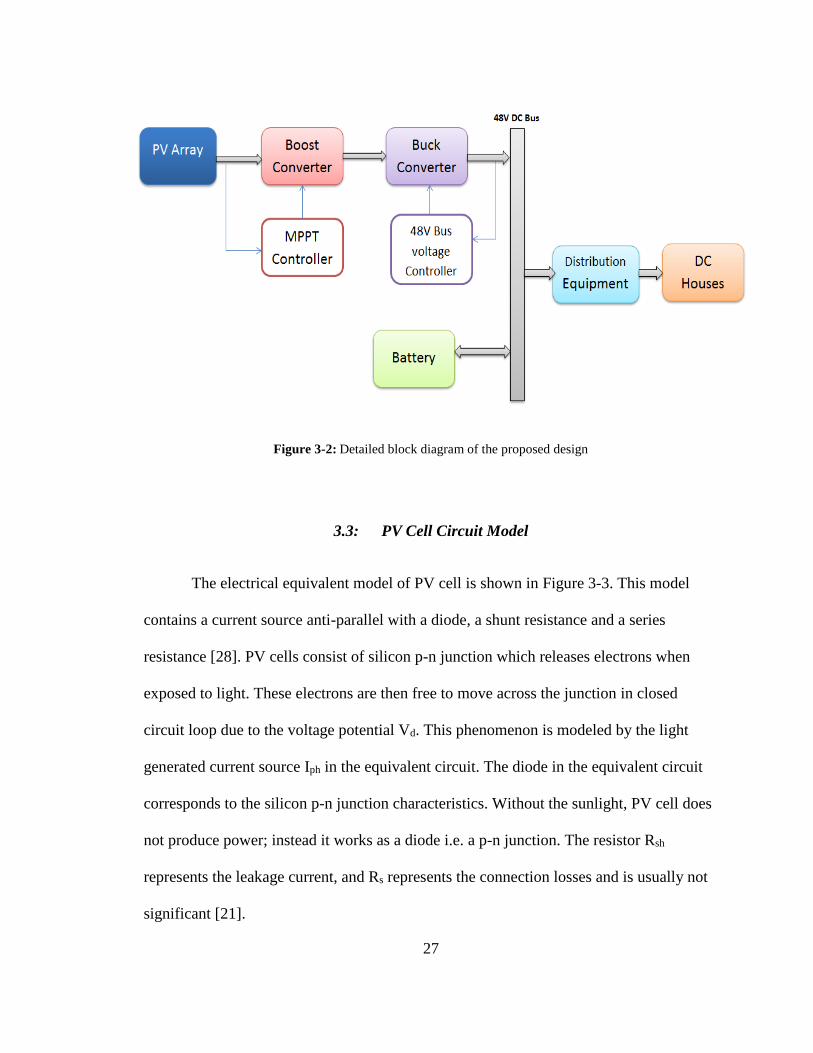
Figure 3-2 illustrates further a detailed block diagram of the proposed system
design. PV array is a constant current source and the main requirement of any switch
mode DC-DC converter used in the MPPT scheme is for it to have low input current
ripple. Buck Converter or its derived topologies has a switch at the input which leads to
higher input current ripple and requires a big capacitor at the input. On the other hand, the
input current for a Boost Converter is continuous due to the inductor at the input.
Therefore, Boost Converter topology is a better choice for the MPPT scheme. The second
DC-DC converter in the system needs to convert the varying output voltage of the Boost
Converter to a stable 48V DC bus distribution voltage. Additionally this converter must
have low output current ripple, so smooth power is delivered to the DC bus. The Buck
Converter topology fulfills both of these requirements. It has low output current ripple
due to the inductor at its output. The following sections will discuss each component
operation in further detail.
27
Figure 3-2: Detailed block diagram of the proposed design
3.3: PV Cell Circuit Model
The electrical equivalent model of PV cell is shown in Figure 3-3. This model
contains a current source anti-parallel with a diode, a shunt resistance and a series
resistance [28]. PV cells consist of silicon p-n junction which releases electrons when
exposed to light. These electrons are then free to move across the junction in closed
circuit loop due to the voltage potential Vd. This phenomenon is modeled by the light
generated current source Iph in the equivalent circuit. The diode in the equivalent circuit
corresponds to the silicon p-n junction characteristics. Without the sunlight, PV cell does
not produce power; instead it works as a diode i.e. a p-n junction. The resistor Rsh
represents the leakage current, and Rs represents the connection losses and is usually not
significant [21].
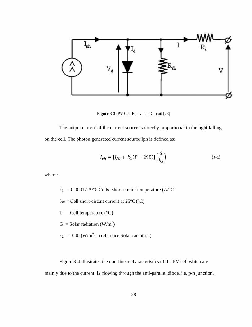
28
Figure 3-3: PV Cell Equivalent Circuit [28]
The output current of the current source is directly proportional to the light falling
on the cell. The photon generated current source Iph is defined as:
𝐼𝑝ℎ = [𝐼𝑆𝐶 + 𝑘1(𝑇 − 298)] (𝐺
𝑘2) (3-1)
where:
k1 = 0.00017 A/ Cells’ short-circuit temperature (A/°C)
ISC = Cell short-circuit current at 25 (°C)
T = Cell temperature (°C)
G = Solar radiation (W/m2)
k2 = 1000 (W/m2), (reference Solar radiation)
Figure 3-4 illustrates the non-linear characteristics of the PV cell which are
mainly due to the current, Id, flowing through the anti-parallel diode, i.e. p-n junction.

29
Figure 3-4: The I-V characteristics of a PV cell [21]
The basic equation to characterize the solar cell I-V relationship is derived from
analyzing the equivalent circuit in Figure 3-3. The following equation is obtained using
circuit’s Kirchoff’s current law:
𝐼 = 𝐼𝑝ℎ − 𝐼𝑑 − 𝐼𝑠ℎ (3-2)
Next, the substitution of relevant expressions for the diode current Id and the shunt
branch current Ish provides equation 3-3:
𝐼 = 𝐼𝑝ℎ − 𝐼𝑠𝑑 [𝑒𝑥𝑝 (
𝑉 + 𝐼𝑅𝑠
𝑛𝑘𝑇𝑞
) − 1] − (𝑉 + 𝐼𝑅𝑠
𝑅𝑠ℎ) (3-3)
where:
Isd = diode’s saturation current (A)
k = 1.3807 × 10⁻²³, Boltzmann constant, (JK-1)
q = 1.6022 × 10⁻¹⁹, electric charge, (C)
n = diode’s quality factor
30
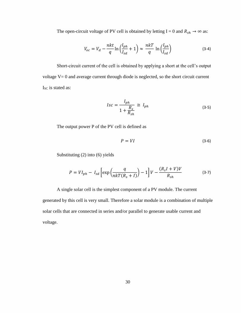
The open-circuit voltage of PV cell is obtained by letting I = 0 and 𝑅𝑠ℎ → ∞ as:
𝑉𝑜𝑐 = 𝑉𝑑 −𝑛𝑘𝑡
𝑞ln (
𝐼𝑝ℎ
𝐼𝑠𝑑+ 1) ≈
𝑛𝑘𝑇
𝑞 ln (
𝐼𝑝ℎ
𝐼𝑠𝑑 ) (3-4)
Short-circuit current of the cell is obtained by applying a short at the cell’s output
voltage V= 0 and average current through diode is neglected, so the short circuit current
ISC is stated as:
𝐼𝑠𝑐 =
𝐼𝑝ℎ
1 +𝑅𝑠
𝑅𝑠ℎ
≅ 𝐼𝑝ℎ (3-5)
The output power P of the PV cell is defined as
𝑃 = 𝑉𝐼 (3-6)
Substituting (2) into (6) yields
𝑃 = 𝑉𝐼𝑝ℎ − 𝐼𝑠𝑑 [exp (𝑞
𝑛𝑘𝑇(𝑅𝑠 + 𝐼)) − 1] 𝑉 −
(𝑅𝑠𝐼 + 𝑉)𝑉
𝑅𝑠ℎ (3-7)
A single solar cell is the simplest component of a PV module. The current
generated by this cell is very small. Therefore a solar module is a combination of multiple
solar cells that are connected in series and/or parallel to generate usable current and
voltage.

31
3.3.1: PV module PSCAD Implementation
Figure 3-5 illustrates the custom library component, available in PSCAD, to
emulate PV behavior. This component was developed by Dr. Athula Rajapakse from the
University of Manitoba, Canada. This module implements behavior of equation 3-3 based
on temperature and irradiance inputs. Figure 3-6 illustrates the default parameters of the
individual PV cell that were used in the simulation. One can obtain these parameters from
PV manufacturer’s data sheet, and modify them accordingly in the PSCAD to emulate the
behavior of a particular PV cell that will be used.
Figure 3-5: PV Module Components available in PSCAD

32
Figure 3-6: PV Cell Default Parameters
Figure 3-7 illustrates the PV array configuration used for the simulation. In the
PV array parameters, one can change the number of cells in a module in series or parallel
configuration as well as can configure the PV array with series or parallel connect PV
modules as needed. The Standard Operating Condition (SOC) test for PV is performed at
800 W/m2 and 25°C. The SOC I-V and Power characteristics of the individual module
used in the simulation are shown in Figure 3-8. The power generation of the module
varies with the operating voltage and maximum power generation point occurs around the
knee of the curve when module is operating around 24V. In this configuration 400 PV
panels are connected in parallel. A single panel could produce 45W of maximum power,
which means in this configuration PV array is capable of producing 18kW of power.
33
Figure 3-7: PV Module and PV Array Parameters
1.
Figure 3-8: PV Module I-V and Power Characteristics
34
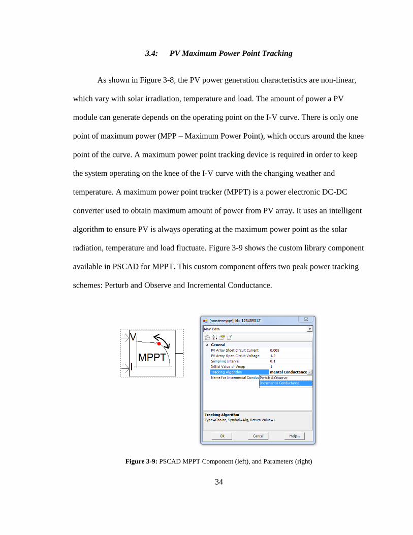
3.4: PV Maximum Power Point Tracking
As shown in Figure 3-8, the PV power generation characteristics are non-linear,
which vary with solar irradiation, temperature and load. The amount of power a PV
module can generate depends on the operating point on the I-V curve. There is only one
point of maximum power (MPP – Maximum Power Point), which occurs around the knee
point of the curve. A maximum power point tracking device is required in order to keep
the system operating on the knee of the I-V curve with the changing weather and
temperature. A maximum power point tracker (MPPT) is a power electronic DC-DC
converter used to obtain maximum amount of power from PV array. It uses an intelligent
algorithm to ensure PV is always operating at the maximum power point as the solar
radiation, temperature and load fluctuate. Figure 3-9 shows the custom library component
available in PSCAD for MPPT. This custom component offers two peak power tracking
schemes: Perturb and Observe and Incremental Conductance.
Figure 3-9: PSCAD MPPT Component (left), and Parameters (right)
35
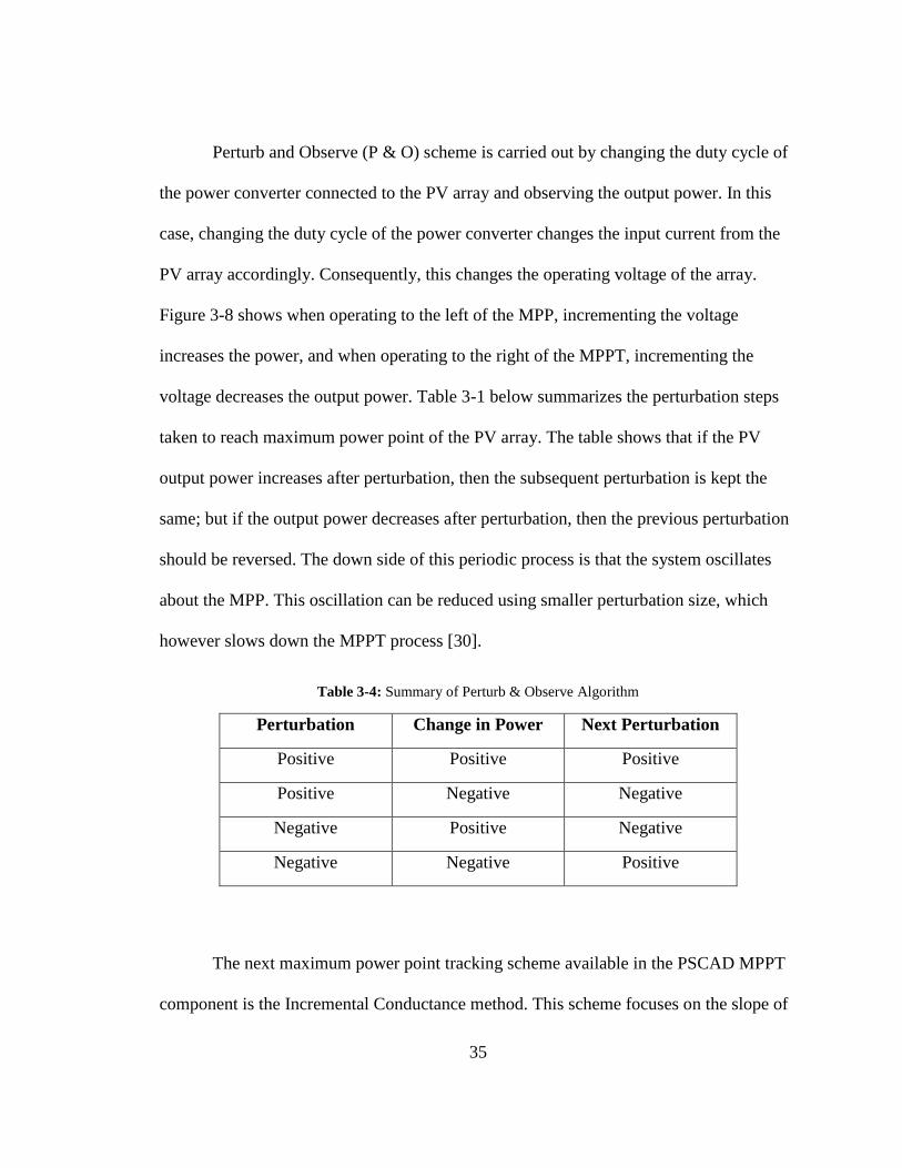
Perturb and Observe (P & O) scheme is carried out by changing the duty cycle of
the power converter connected to the PV array and observing the output power. In this
case, changing the duty cycle of the power converter changes the input current from the
PV array accordingly. Consequently, this changes the operating voltage of the array.
Figure 3-8 shows when operating to the left of the MPP, incrementing the voltage
increases the power, and when operating to the right of the MPPT, incrementing the
voltage decreases the output power. Table 3-1 below summarizes the perturbation steps
taken to reach maximum power point of the PV array. The table shows that if the PV
output power increases after perturbation, then the subsequent perturbation is kept the
same; but if the output power decreases after perturbation, then the previous perturbation
should be reversed. The down side of this periodic process is that the system oscillates
about the MPP. This oscillation can be reduced using smaller perturbation size, which
however slows down the MPPT process [30].
Table 3-4: Summary of Perturb & Observe Algorithm
Perturbation Change in Power Next Perturbation
Positive Positive Positive
Positive Negative Negative
Negative Positive Negative
Negative Negative Positive
The next maximum power point tracking scheme available in the PSCAD MPPT
component is the Incremental Conductance method. This scheme focuses on the slope of

36
the PV array power curve. The slope of the PV array power curve is zero at the MPP,
positive on the left of the MPP and negative on the right, as given by:
dP/dV = 0, at MPP
dP/dV > 0, left of MPP
dP/dV < 0, right of MPP
(3-8)
Since
𝑑𝑃
𝑑𝑉=
𝑑 (𝐼𝑉)
𝑑𝑉= 𝐼 + 𝑉
𝑑𝐼
𝑑𝑉≅ 𝐼 + 𝑉
∆𝐼
∆𝑉 (3-9)
Equation 3-8 can be rewritten as:
∆I/∆V = -I/V, at MPP
∆I/∆V > -I/V, left of MPP
∆I/∆V < -I/V, right of MPP
(3-10)
Therefore, MPP can be tracked by comparing the instantaneous conductance (I/V)
with the incremental conductance (∆I/∆V). Figure 3-10 illustrates the incremental
conductance base algorithm used by the PSCAD MPPT component. The operating point
of the PV array is Vref which is equal to Vmpp at MPP. Once MPP has been reached, the
PV array is maintained at this point unless a change in ∆I is noted. No oscillation around
the MPP point is the advantage incremental conductance has over P & O algorithm.
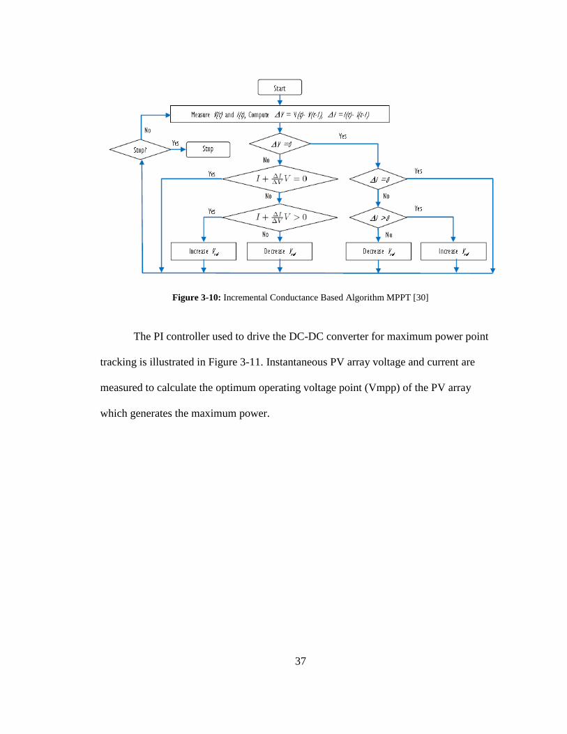
37
Figure 3-10: Incremental Conductance Based Algorithm MPPT [30]
The PI controller used to drive the DC-DC converter for maximum power point
tracking is illustrated in Figure 3-11. Instantaneous PV array voltage and current are
measured to calculate the optimum operating voltage point (Vmpp) of the PV array
which generates the maximum power.

38
Figure 3-11: The Controller used to drive the Boost Converter Switch for MPPT
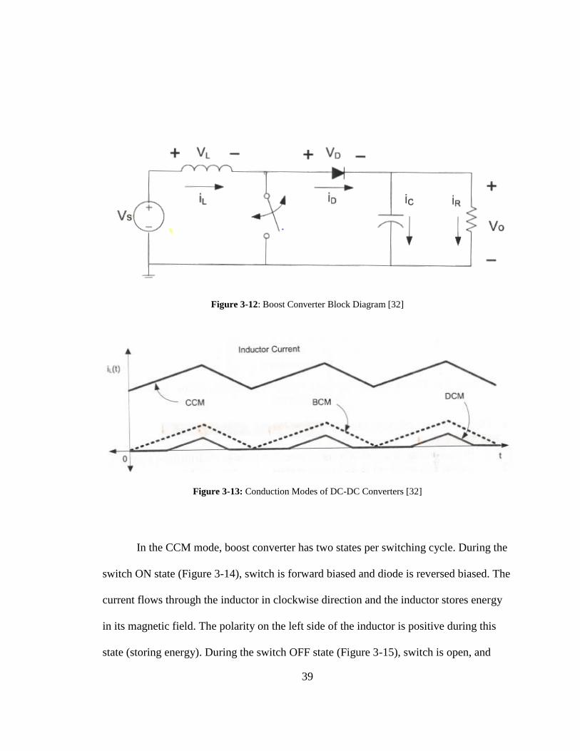
3.5: Boost Converter Operation
Figure 3-12 illustrates the basic block diagram of the Boost Converter. DC-DC
converters can operate in three conduction modes: Continuous Conduction Mode (CCM),
Discontinuous Conduction Mode (DCM), and Boundary Conduction Mode (BCM) [32].
In Continuous Conduction Mode, the inductor current remains positive throughout the
switching period. In Discontinuous Conduction Mode, the inductor current reaches zero
for portion of the switching period. In Boundary Conduction Mode, the inductor current
is at the edge of the CCM before going to the DCM (special case of CCM). Figure 3-13
illustrates the three different conduction modes of the DC-DC converters. Since the Boost
Converter will be connected to the PV array (constant current source), the desired mode
of operation for the converter is the Continuous Conduction Mode.
39
Figure 3-12: Boost Converter Block Diagram [32]
Figure 3-13: Conduction Modes of DC-DC Converters [32]
In the CCM mode, boost converter has two states per switching cycle. During the
switch ON state (Figure 3-14), switch is forward biased and diode is reversed biased. The
current flows through the inductor in clockwise direction and the inductor stores energy
in its magnetic field. The polarity on the left side of the inductor is positive during this
state (storing energy). During the switch OFF state (Figure 3-15), switch is open, and

40
diode is forward biased, which increases the impedance of the circuit. Consequently the
inductor resists the change in the circuit current due to higher impedance; thus the
polarity of the inductor is reversed (positive polarity on the right side of the inductor). As
a result two sources in series supply the load at higher voltage and charge the output
capacitor simultaneously. Also the output capacitor is sized to supply sufficient power to
the load during the switch OFF state [33].
Figure 3-14: Boost Converter CCM Switch ON State [32]
The voltage across the inductor during switch ON state can be written as:
𝑉𝐿 = 𝑉𝑆 = 𝐿𝑑𝑖𝐿
𝑑𝑡 𝑜𝑟
𝑑𝑖𝐿
𝑑𝑡=
𝑉𝑆
𝐿 (3-11)
The increasing inductor current during the switch ON state is given by:
𝑑𝑖𝐿
𝑑𝑡 =
∆𝑖𝐿
∆𝑡=
∆𝑖𝐿
𝐷𝑇=
𝑉𝑆
𝐿 (3-12)

41
∆𝑖𝐿−𝐶𝑙𝑜𝑠𝑒𝑑 =𝑉𝑆
𝐿 𝐷𝑇 (3-13)
Figure 3-15: Boost Converter CCM Switch OFF State [32]
The voltage across the inductor during switch OFF is calculated as:
𝑉𝐿 = 𝑉𝑠 − 𝑉𝑂 (3-14)
𝑉𝐿 = 𝐿 𝑑𝑖𝐿
𝑑𝑡 𝑜𝑟
𝑑𝑖𝐿
𝑑𝑡=
𝑉𝑆 − 𝑉𝑜
𝐿 (3-15)
The change in the inductor current is computed as:
𝑑𝑖𝐿
𝑑𝑡=
∆𝑖𝐿
∆𝑡=
∆𝑖𝐿
(1 − 𝐷)𝑇=
𝑉𝑆 − 𝑉𝑂
𝐿 (3-16)
∆𝑖𝐿−𝑂𝑝𝑒𝑛 =(𝑉𝑆 − 𝑉𝑂)(1 − 𝐷)𝑇
𝐿 (3-17)
42
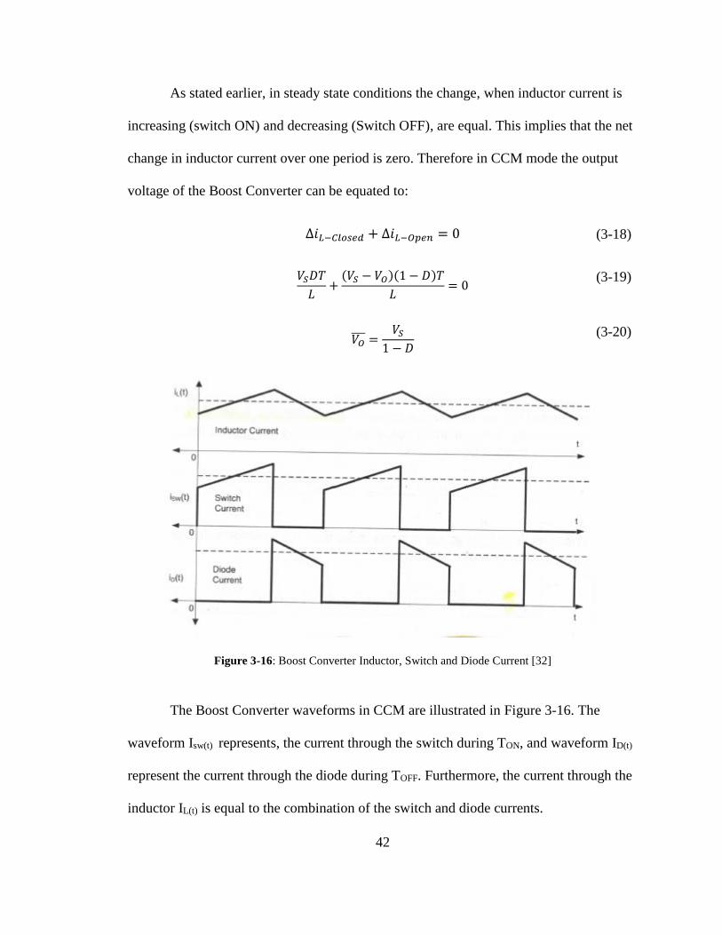
As stated earlier, in steady state conditions the change, when inductor current is
increasing (switch ON) and decreasing (Switch OFF), are equal. This implies that the net
change in inductor current over one period is zero. Therefore in CCM mode the output
voltage of the Boost Converter can be equated to:
∆𝑖𝐿−𝐶𝑙𝑜𝑠𝑒𝑑 + ∆𝑖𝐿−𝑂𝑝𝑒𝑛 = 0 (3-18)
𝑉𝑆𝐷𝑇
𝐿+
(𝑉𝑆 − 𝑉𝑂)(1 − 𝐷)𝑇
𝐿= 0
(3-19)
𝑉𝑂 =
𝑉𝑆
1 − 𝐷
(3-20)
Figure 3-16: Boost Converter Inductor, Switch and Diode Current [32]
The Boost Converter waveforms in CCM are illustrated in Figure 3-16. The
waveform Isw(t) represents, the current through the switch during TON, and waveform ID(t)
represent the current through the diode during TOFF. Furthermore, the current through the
inductor IL(t) is equal to the combination of the switch and diode currents.

43
3.5.1: Boost Converter PSCAD Implementation
Figure 3-17 illustrates the block diagram of Boost Converter implemented in
PSCAD. An input capacitor is used for a stable voltage input from the PV array. The duty
cycle of the switch is controlled by the MPPT controller shown in Figure 3-11. The
MPPT varies the duty cycle according to the solar irradiance, temperature and load
conditions in order to extract maximum power out of the PV array. The switching
frequency of the DC-DC converter can be selected from a range starting at 5 kHz to over
100 kHz. A higher switching frequency requires smaller energy storage components
(inductor and capacitor), which makes the converter compact. However, the trade-off is
that the simulation runs very slow because of the lower time step required by high
switching frequency. As a result, switching frequency of 20 kHz was selected to keep the
balance between the two trade-offs.
Figure 3-17: Boost Converter connected to the PV Array in PSCAD
The critical inductance that yields Continuous Conduction Mode is determined
from the minimum value of inductor current IL-min as:
𝐿𝐶 =𝐷(1 − 𝐷)2𝑅
2𝑓 (3-21)

44
In 3-21 “R” represents the load resistance. Minimum of five DC houses will be
consuming 2.5 kW of power almost entirely. Load in terms of resistance for five houses
is calculated to be:
𝑅 =𝑉2
𝑃=
482
2500= .9216 Ω (3-22)
And, for a 50% duty cycle the Critical inductance is calculated to be:
𝐿𝐶 =. 5(1 − .5)2 ∗ .9218
2 ∗ 20 × 103= 2.88 µ𝐻 (3-23)
The duty cycle of the converter varies according to the weather and load
conditions. Therefore, a higher value for the inductor is preferred to ensure that the
converter is working in CCM mode at all time. The inductor of 20µH was tested and
chosen to keep the converter in CCM mode under varying weather and load conditions.
The output capacitor value is determined by:
𝐶 =𝐷
𝑅𝑓×
𝑉𝑂
∆𝑉𝑂 (3-24)
A 50% duty cycle at 25V input voltage will boost the output voltage to 50V, and
the output capacitor required in this case would be:
𝐶 =. 5
. 1884 ∗ 20 × 103×
50
1= 6.7 𝑚𝐹 (3-25)
The output voltage ripple has an inverse relationship with the output capacitor
value, so a lower output ripple will require a bigger capacitor. As mentioned, this

45
converter will have varying duty cycle according to the different weather and load
conditions. A 10 mf capacitor was chosen for different operating conditions.
3.6: Buck Converter Operation
As mentioned earlier, the second DC-DC converter in the system needs to convert
the varying output voltage of the Boost Converter to a stable 48V DC bus distribution
voltage. Additionally this converter must have low output current ripple, so smooth
power is delivered to the DC bus. The Buck Converter topology fulfills both of these
requirements. It has low output current ripple due to the inductor’s location in the circuit,
as illustrated in Figure 3-18 [32]. The cascading of Boost and Buck converter provides
good input and output current characteristics. As mentioned in the previous section, the
desired mode of operation for these converters is the Continuous Conduction Mode.
Therefore, all the following equations are derived in the Continuous Conduction Mode.
Figure 3-18: Buck Converter Block Diagram [32]

46
Similar to Boost, Buck converter also has two states in the Continuous
Conduction Mode: Switch ON and Switch OFF. In the switch ON state, the diode is
reverse biased (Figure 3-19), and the voltage across the inductor is:
𝑉𝐿 = 𝑉𝑆 − 𝑉𝑂 (3-26)
Figure 3-19: Buck Converter CCM Switch ON State [32]
The change in the inductor current is calculated as:
𝑑𝑖𝐿𝑡
𝑑𝑡=
∆𝑖𝐿
∆𝑡=
∆𝑖𝐿
𝐷𝑇=
𝑉𝑆 − 𝑉𝑂
𝐿 (3-27)
∆𝑖𝐿−𝑐𝑙𝑜𝑠𝑒𝑑 =
(𝑉𝑆 − 𝑉𝑂)
𝐿 𝐷𝑇
(3-28)
The second state of the Buck converter is illustrated in Figure 3-20. In this state
switch is turned off and the voltage across inductor is:
𝑉𝐿 = −𝑉0 = 𝐿𝑑𝑖𝐿
𝑑𝑡 (3-29)

47
Figure 3-20: Buck Converter CCM Switch OFF State [32]
The change in the inductor current is computed as:
∆𝑖𝐿
𝑡𝑜𝑓𝑓=
∆𝑖𝐿
𝑇 − 𝐷𝑇=
∆𝑖𝐿
(1 − 𝐷)𝑇= −
𝑉𝑂
𝐿 (3-30)
∆𝑖𝐿−𝑜𝑝𝑒𝑛 = −𝑉𝑂
𝐿(1 − 𝐷)𝑇 (3-31)
In steady state operation the net change in the inductor current is zero. Therefore
the output voltage of the Buck Converter is:
∆𝑖𝐿−1𝑝𝑒𝑟𝑖𝑜𝑑 = ∆𝑖𝐿−𝑐𝑙𝑜𝑠𝑒𝑑 + ∆𝑖𝐿−𝑜𝑝𝑒𝑛 = 0 (3-40)
0 =
𝑉𝑆 − 𝑉𝑂
𝐿𝐷𝑇 −
𝑉𝑂
𝐿(1 − 𝐷)𝑇
(3-41)
0 =
𝑉𝑠
𝐿𝐷𝑇 −
𝑉𝑜
𝐿𝐷𝑇 −
𝑉𝑂
𝐿𝑇 +
𝑉𝑜
𝐿𝐷𝑇
(3-42)
𝑉𝑜 = 𝐷𝑉𝑆 (3-43)

48
Figure 3-21: Buck Converter CCM Waveforms [34]
The Buck Converter waveforms are shows in Figure 3-21. As mentioned earlier,
when the switch is ON, the inductor current increases linearly and capacitor is charged.
And, when the switch is OFF, the inductor current decrease linearly and capacitor
discharges to supply the load. The net change in the inductor current in the steady state is
zero. The output voltage ripple is a function of the output capacitor. A bigger capacitor at
the output will result in low ripple in the output voltage ripple [32].

49
3.6.1: Buck Converter PSCAD implementation
In PSCAD the Buck Converter is cascaded with the Boost Converter as shown in
Figure 3-22. The output voltage of the Buck Converter is regulated at 48V while the input
voltage varies depending on the solar irradiance, temperature and load. Figure 3-23
illustrates the PI controller used for the output voltage regulation. In order to get a
regulated 48V at the DC bus, the controller compares the output voltage of the Buck
Converter (DC bus voltage) to the reference 48V. If the output voltage is lower than 48V,
the switch turns on to charge the output capacitor; if the output voltage is higher than
48V, the switch turns off to discharge the output capacitor. The switching frequency of
the converter is 20 kHz.
Figure 3-22: Buck Converter Cascaded with Boost Converter in PSCAD

50
Figure 3-23: Buck Converter Switch Controller for Regulating Output Voltage at 48V
The critical inductance of the converter is computed as:
𝐿𝐶 =(1 − 𝐷) 𝑅𝑚𝑎𝑥
2𝑓 (3-44)
𝐿𝐶 = (1 − .5) ∗ .9218
2 ∗ 20000= .011𝑚𝐻
But a .1mH was selected because the load resistance can go higher and duty cycle
can go lower under different test conditions.
The minimum capacitor required at the output is computed as:
𝐶𝑂 =1 − 𝐷
∆𝑉𝑉𝑜
8𝐿𝑓2 (3-45)
𝐶𝑜 =1 − .2
148 8 (. 0001)(20000)2
= .12𝑚𝑓 (3-46)

51
3.7: Battery Bank
PV power generation varies with the amount of sunlight shining on the panels at
an instance, which results in lack of power generation during night time and cloudy
weather. At such times, a battery bank is needed in order to provide smooth power to the
load continuously. There are four major types of rechargeable batteries used as energy
storing devices: Lead Acid, Nickel-51Cadmium (NiCD), Nickel-metal-hydride (NiMH),
Lithium-ion (Li-ion). Figure 3-25 shows the discharge characteristics of an individual cell
for the batteries.
Figure 3-25: Cell Discharge Characteristics of Four Battery Types
In order to determine the optimal battery type, the major attributes to focus on are
the specific energy, years of service life, load characteristics, price, safety, self-discharge,
environmental issues, and disposal. NiCD, NiMH, and Li-ion batteries are usually used in

52
critical and extreme temperature applications [23]. However the reason they are not likely
candidates for use in PV systems is because their high initial costs and unavailability
offset their advantageous characteristics.
Lead Acid batteries are one of the oldest rechargeable battery systems created by
French Physicist Gaston Plante in 1859 [24]. Their low cost, high tolerance to over-
charge and over-discharge characteristics make them ideal for isolated PV systems. There
are three different types of lead acid batteries available in the market today: flooded lead-
acid, gelled electrolyte, and absorbed glass mat (AGM). Gelled electrolyte and AGM are
also commonly referred to as sealed or valve-regulated lead acid batteries (VRLA). The
advantages and disadvantages of these two different battery types are compared in Table
3-2.
Table 3-2: Comparison of Flooded Lead-Acid and VRLA Battery Types [23]

53
These Gelled and AGM (VRLA) batteries are designed to minimize the required
maintenance over the life of the battery. In the small PV systems, VRLAs are the most
popular because of their low maintenance requirements, even though their cost is higher
than the Flooded Lead-Acid batteries. Other differentiating attributes include the
impossibility of adding an electrolyte to the VRLA batteries due to their seal construction
type. The sealed construction makes VRLA batteries extremely intolerant to
overcharging and high temperatures [23]. Hence, the Flooded Lead-acid batteries are the
most ideal battery type for the centralized DC House distribution system. In the next
section, the implementation of Lead-acid battery model is discussed.
3.7.1: Battery Bank PSCAD Implementation
The battery is modeled by a controlled voltage source in series with a constant
resistance, as shown in Figure 3-26.
Figure 3-26: Battery Equivalent Circuit Diagram [18]

54
This basic equivalent battery circuit is represented by shepherd’s equation as:
𝐸𝑏𝑎𝑡 = 𝐸𝑂 − 𝐾 ∗(1 − 𝑆𝑂𝐶)
𝑆𝑂𝐶∗ 𝑄 + 𝐴𝑒−𝐵(1−𝑆𝑂𝐶)𝑄 (3-46)
The voltage at the battery terminal is calculated as:
𝑉𝑏𝑎𝑡 = 𝐸𝑏𝑎𝑡 − 𝑅𝑏𝑎𝑡 ∗ 𝐼𝑏𝑎𝑡 (3-47)
where:
Ebat: internal voltage (V)
Eo: battery voltage constant (V)
K: polarization constant (V/Ah) or polarization resistance (Ω)
SOC : State of charge (%)
Q: battery capacity (Ah)
A: exponential Zone amplitude (V)
B: exponential zone time constant inverse (1/Ah)
Vbat: terminal voltage (V)
Ibat: battery current (A)
Figure 3-27 illustrate the custom battery component available in PSCAD, which
implements equation 3-46.
Figure 3-27: Battery Custom Component in available in PSCAD
55
where:
Ibat: The current of the battery, input signal.
Reset: The control signal used to control charge or discharge of the
battery, input signal.
SOC: State of charger, output signal
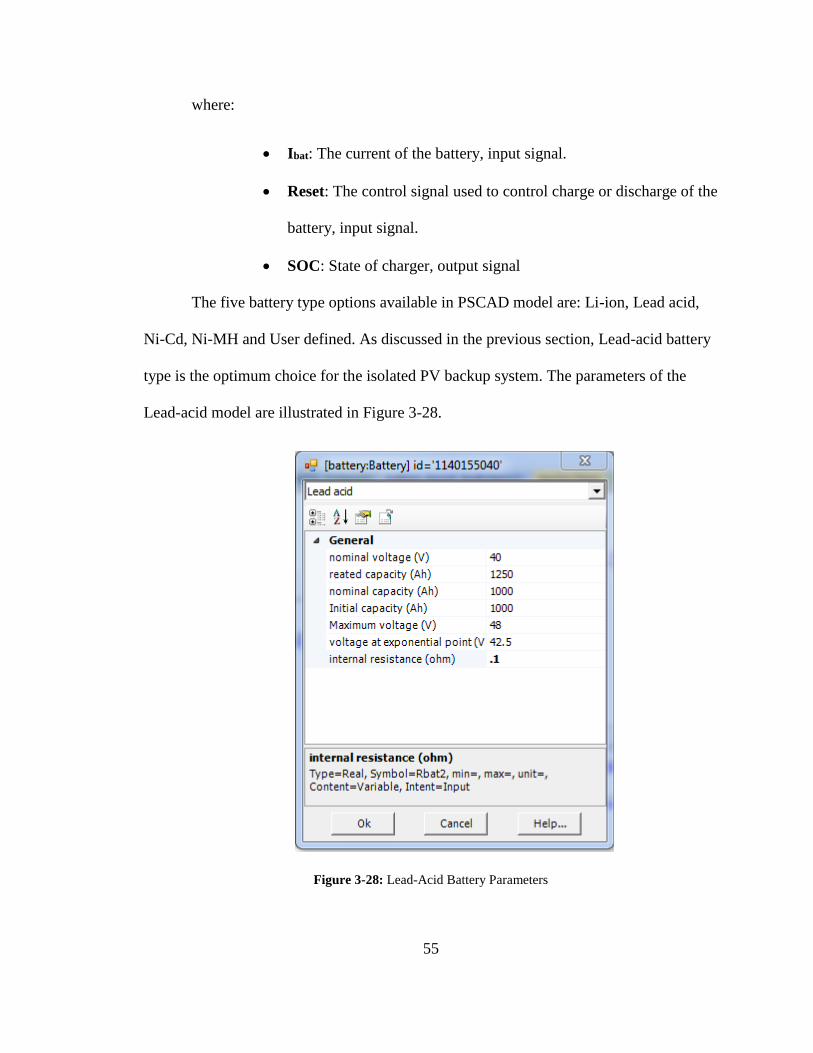
The five battery type options available in PSCAD model are: Li-ion, Lead acid,
Ni-Cd, Ni-MH and User defined. As discussed in the previous section, Lead-acid battery
type is the optimum choice for the isolated PV backup system. The parameters of the
Lead-acid model are illustrated in Figure 3-28.
Figure 3-28: Lead-Acid Battery Parameters

56
Nominal Voltage (V): End of the linear zone of the discharge characteristics
Rated Capacity (Ah): Rated capacity of the battery
Initial Capacity (Ah): Initial condition for the simulation and does not affect
the discharge curve
Nominal capacity (Ah): The amount of current that can be extracted from the
battery before it needs to recharge
Voltage at exponential point (V): The exponential point corresponds to the
end of the exponential zone
Maximum Voltage (V): Battery voltage when its fully charged
Internal Resistance (Ω): Internal resistance of the battery
The voltage of battery cell varies in accordance with its charge state (Figure 3-
25). Similarly, the terminal voltage of the battery bank will decrease as its SOC (state of
charge) goes down. But the battery bank needs supply power to the load consistently at
48V during the non-generation periods. A DC-DC converter with regulated output helps
to meet this design requirement. Figure 3-29 illustrates the battery bank design
implemented in PSCAD. The top path is used for charging the battery and it is
discharged through the bottom path. Boost Converter (sub-module “Boost-Bat1”) steps-
up the battery terminal voltage to 48V DC Bus voltage when the load is supplied from
the battery. Figure3-30 illustrates the Boost Converter and controller with-in the sub-
module.

57
Figure 3-29: Complete Battery Bank Design
Figure 3-30: Boost Converter (top) and Controller (bottom) within the Sub-Module Battery Cascaded

58
3.8: Distribution Network
The centralized distribution network for the DC houses is illustrated in Figure 3-
31. This network consists of overhead distribution cables, five feeders and a total of 25
DC houses. The layout is modeled in PSCAD using common feeder characteristics that
system planners use in suburban residential regions [15]. Figure 32 illustrates a magnified
view of individual feeder with five houses. A single DC House load can be varied from
100-500W.
Figure 3-31: Distribution Network Design for 25 DC Houses
Power
supplied
from PV
or Battery
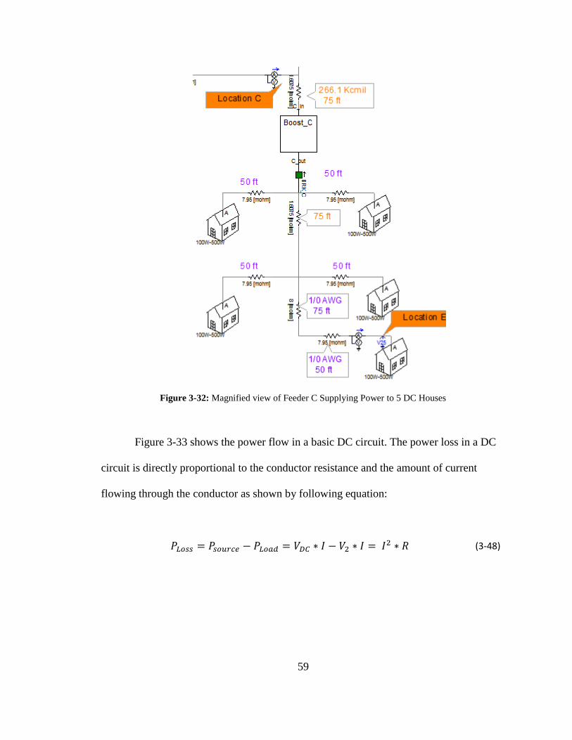
59
Figure 3-32: Magnified view of Feeder C Supplying Power to 5 DC Houses
Figure 3-33 shows the power flow in a basic DC circuit. The power loss in a DC
circuit is directly proportional to the conductor resistance and the amount of current
flowing through the conductor as shown by following equation:
𝑃𝐿𝑜𝑠𝑠 = 𝑃𝑠𝑜𝑢𝑟𝑐𝑒 − 𝑃𝐿𝑜𝑎𝑑 = 𝑉𝐷𝐶 ∗ 𝐼 − 𝑉2 ∗ 𝐼 = 𝐼2 ∗ 𝑅 (3-48)

60
Figure 3-33: DC Equivalent Circuit Diagram [8]
At full load, the minimum current will be:
𝐼𝑓𝑢𝑙𝑙−𝑙𝑜𝑎𝑑 =𝑃
𝑉𝐷𝐶−𝐵𝑢𝑠=
25 ∗ 500
48 = 260.42𝐴 (3-49)
Equation 3-49 shows distribution network will have high currents due to the low
distribution voltage, therefore minimum resistance is desired in the distribution
conductors in order to minimize distribution loses. Aluminum Conductor Steel
Reinforced (ACSR) cables are frequently used for overhead power distribution. Their
performance is highly reliable for many years even under adverse weather conditions.
Table 3-3 shows the characteristics of the different ACSR cables. Waxing conductor at
266.9 kcmill is selected based on the ampacity rating, DC resistance, and cost. The cable
distances labeled in orange (Figure 3-31) corresponds to Waxwing conductor type. The
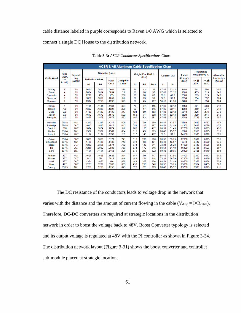
61
cable distance labeled in purple corresponds to Raven 1/0 AWG which is selected to
connect a single DC House to the distribution network.
Table 3-3: ASCR Conductor Specifications Chart
The DC resistance of the conductors leads to voltage drop in the network that
varies with the distance and the amount of current flowing in the cable (Vdrop = I×Rcable).
Therefore, DC-DC converters are required at strategic locations in the distribution
network in order to boost the voltage back to 48V. Boost Converter typology is selected
and its output voltage is regulated at 48V with the PI controller as shown in Figure 3-34.
The distribution network layout (Figure 3-31) shows the boost converter and controller
sub-module placed at strategic locations.
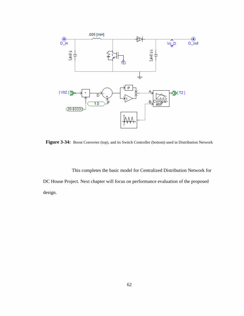
62
Figure 3-34: Boost Converter (top), and its Switch Controller (bottom) used in Distribution Network
This completes the basic model for Centralized Distribution Network for
DC House Project. Next chapter will focus on performance evaluation of the proposed
design.
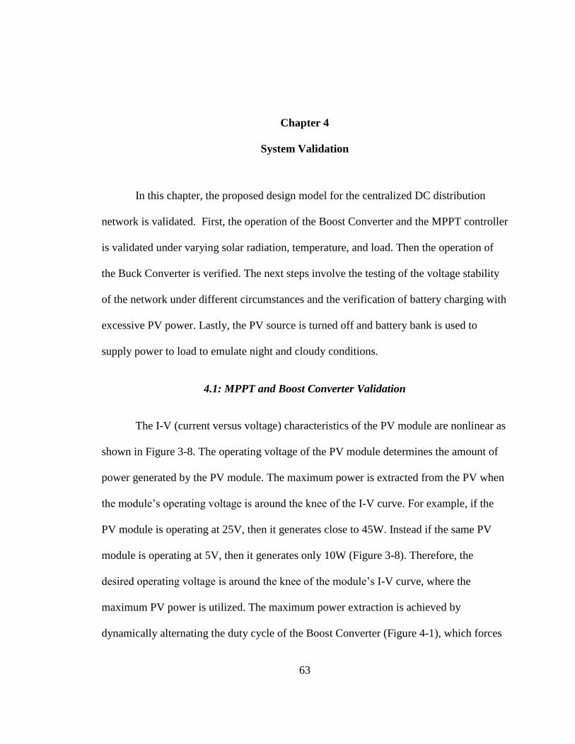
63
Chapter 4
System Validation
In this chapter, the proposed design model for the centralized DC distribution
network is validated. First, the operation of the Boost Converter and the MPPT controller
is validated under varying solar radiation, temperature, and load. Then the operation of
the Buck Converter is verified. The next steps involve the testing of the voltage stability
of the network under different circumstances and the verification of battery charging with
excessive PV power. Lastly, the PV source is turned off and battery bank is used to
supply power to load to emulate night and cloudy conditions.
4.1: MPPT and Boost Converter Validation
The I-V (current versus voltage) characteristics of the PV module are nonlinear as
shown in Figure 3-8. The operating voltage of the PV module determines the amount of
power generated by the PV module. The maximum power is extracted from the PV when
the module’s operating voltage is around the knee of the I-V curve. For example, if the
PV module is operating at 25V, then it generates close to 45W. Instead if the same PV
module is operating at 5V, then it generates only 10W (Figure 3-8). Therefore, the
desired operating voltage is around the knee of the module’s I-V curve, where the
maximum PV power is utilized. The maximum power extraction is achieved by
dynamically alternating the duty cycle of the Boost Converter (Figure 4-1), which forces
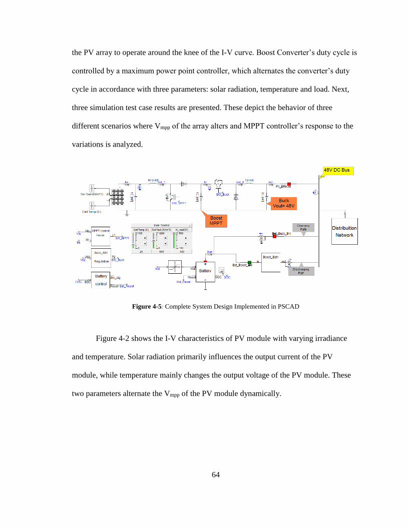
64
the PV array to operate around the knee of the I-V curve. Boost Converter’s duty cycle is
controlled by a maximum power point controller, which alternates the converter’s duty
cycle in accordance with three parameters: solar radiation, temperature and load. Next,
three simulation test case results are presented. These depict the behavior of three
different scenarios where Vmpp of the array alters and MPPT controller’s response to the
variations is analyzed.
Figure 4-5: Complete System Design Implemented in PSCAD
Figure 4-2 shows the I-V characteristics of PV module with varying irradiance
and temperature. Solar radiation primarily influences the output current of the PV
module, while temperature mainly changes the output voltage of the PV module. These
two parameters alternate the Vmpp of the PV module dynamically.
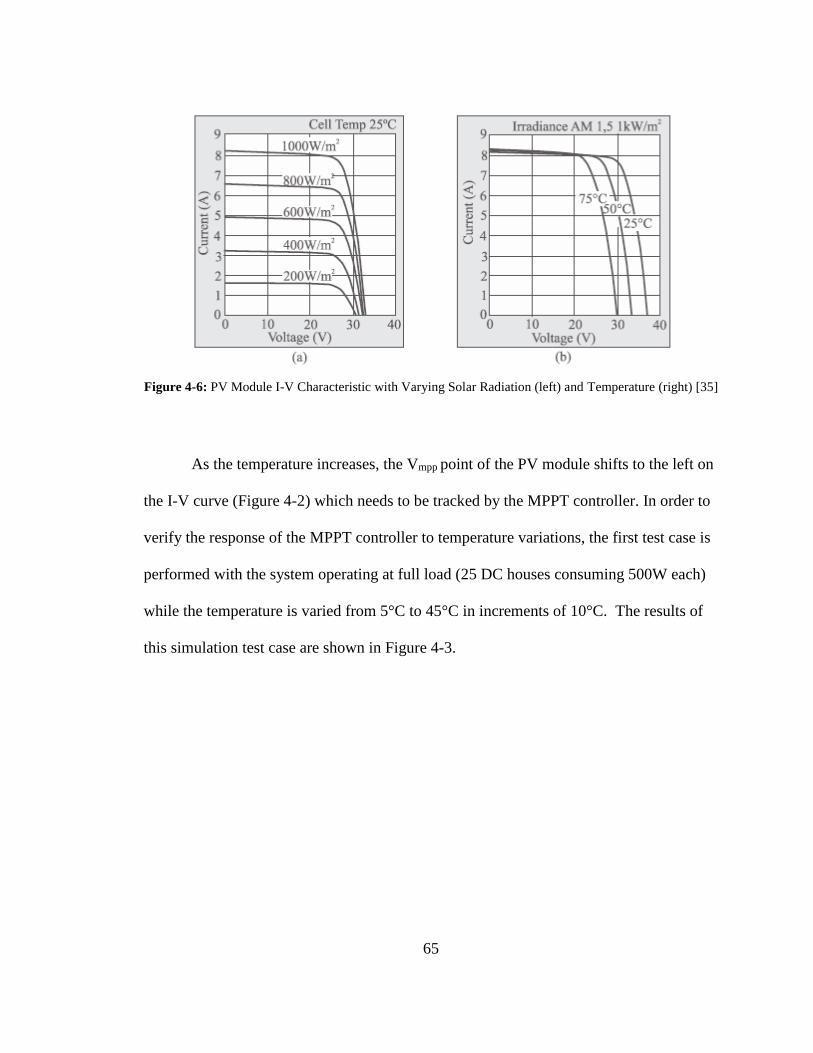
65
Figure 4-6: PV Module I-V Characteristic with Varying Solar Radiation (left) and Temperature (right) [35]
As the temperature increases, the Vmpp point of the PV module shifts to the left on
the I-V curve (Figure 4-2) which needs to be tracked by the MPPT controller. In order to
verify the response of the MPPT controller to temperature variations, the first test case is
performed with the system operating at full load (25 DC houses consuming 500W each)
while the temperature is varied from 5°C to 45°C in increments of 10°C. The results of
this simulation test case are shown in Figure 4-3.

66
Figure 4-7: PV Array output Voltage (top), Current (middle), and Power (bottom) with Varying
Temperature
Table 4-5: PV Output Voltage, Current, and Power with Varying Temperature
Time (seconds) Temperature (°C) Vmpp (V) Current
(A)
Power (kW)
0.1 5 27.6 608 16.8
0.3 15 26.9 624 16.79
0.5 25 26.3 638 16.8
0.7 35 25.8 651 16.8
0.9 45 25.15 668 16.8

67
Table 4-1 summarizes the PV voltage, current, and power measurements with
incrementing temperature. The voltage operating point of the PV array shifted to the left
with increasing temperature as anticipated. The dips in the current and power graph
represent the response time of the MPPT controller between the temperature change and
the implementations of the necessary modifications to the Boost Converter’s duty cycle.
For the second simulation test case, solar radiation is varied from 400W/m2 to
1000W/m2 in steps of 200 W/m2, while temperature remains constant at 25°C. The results
of the simulation test case are shown in Figure 4-4.
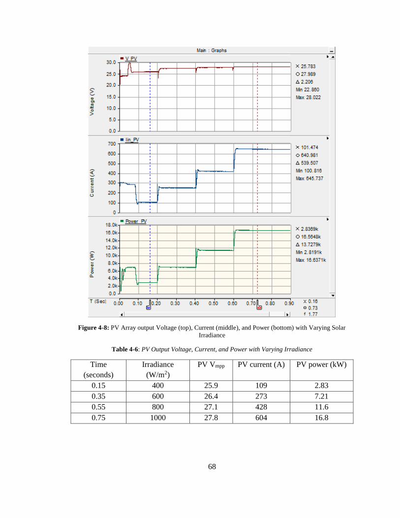
68
Figure 4-8: PV Array output Voltage (top), Current (middle), and Power (bottom) with Varying Solar
Irradiance
Table 4-6: PV Output Voltage, Current, and Power with Varying Irradiance
Time
(seconds)
Irradiance
(W/m2)
PV Vmpp PV current (A) PV power (kW)
0.15 400 25.9 109 2.83
0.35 600 26.4 273 7.21
0.55 800 27.1 428 11.6
0.75 1000 27.8 604 16.8
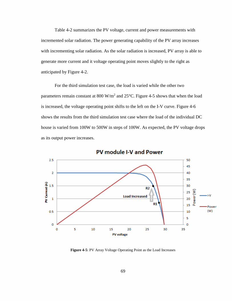
69
Table 4-2 summarizes the PV voltage, current and power measurements with
incremented solar radiation. The power generating capability of the PV array increases
with incrementing solar radiation. As the solar radiation is increased, PV array is able to
generate more current and it voltage operating point moves slightly to the right as
anticipated by Figure 4-2.
For the third simulation test case, the load is varied while the other two
parameters remain constant at 800 W/m2 and 25°C. Figure 4-5 shows that when the load
is increased, the voltage operating point shifts to the left on the I-V curve. Figure 4-6
shows the results from the third simulation test case where the load of the individual DC
house is varied from 100W to 500W in steps of 100W. As expected, the PV voltage drops
as its output power increases.
Figure 4-5: PV Array Voltage Operating Point as the Load Increases

70
Figure 4-6: PV Array operating Voltage (top), Current (middle), and Power (bottom) with Varying Load
Table 4-3: PV Output Voltage, Current and Power with Varying Load
Time (seconds) House Load (W) Vmpp (V) Current
(A)
Power (kW)
0.15 100 29.37 95 2.8
0.25 200 28.98 196 5.68
0.45 300 28.46 318 9.05
0.65 400 27.85 442 12.31
0.85 500 26.70 614 16.4
71
Data from Table 4-3 show that the Vmpp (operating point of the PV array) moves
to the left with increasing load as predicted.
Figure 4-7 depicts the input (PV voltage) and output voltage of the Boost
Converter as the load is increased at standard operating conditions (800W/m^2 @ 25°C).
The output voltage of the Boost Converter is dependent upon its duty cycle, which is
controlled by the MPPT controller. Table 4-4 summarizes the input and output voltages
and duty cycle of the Boost Converters. The duty cycle of the converter is calculated
according to equation 4-1. The duty cycle of the converter decreases as the load increases
which accounts for more power transferred to the output.

72
Figure 4-7: Boost Converter Input and Output Voltages with increasing Load
Table 4-4: Summary of the Boost Converter Voltages and Duty Cycle with Increasing Load
Time (seconds) Load Vmpp (V) Boost Vo (V) Duty Cycle (%)
0.15 100 29.37 147.3 80.1
0.25 200 28.98 143.9 79.9
0.45 300 28.46 139.29 79.56
0.65 400 27.85 134.47 79.29
0.85 500 26.70 126.4 78.87
%𝐷𝑢𝑡𝑦 𝐶𝑦𝑐𝑙𝑒𝐵𝑜𝑜𝑠𝑡 = (1 − 𝑉𝑃𝑉
𝑉𝑜𝐵𝑜𝑜𝑠𝑡) × 100% (4-1)

73
The Continuous Conduction mode of the converter is verified by Figure 4-8. The
top graph (Figure 4-8) shows the increasing current through the inductor as the load
increases. The bottom graph displays a magnified view of the charging and discharging
of the inductor at full load (500W). The inductor is charging for approximately 80% of
the total period and discharging for about 20% of the total period as it was calculated
from the input and output voltages of the converter (Table 4-4). Next, the operation of the
Buck Converter is verified.
Figure 4-8: Boost Converter Inductor Current (top) and Magnified View of Inductor Current at Full Load
(bottom)

74
4.2: Buck Converter Validation
The Buck converter needs to step-down its input voltage (which is the output
voltage of the Boost Converter) to 48V DC bus voltage. Thus, the Buck Converter’s
output is dynamically regulated at 48V by the PI controller. Figure 4-9 depicts the input
and output voltages of the Buck Converter with increasing load. The graph data is
summarized in Table 4-5 and verify that the Buck Converter is regulating its output
voltage at 48V (also the DC bus voltage) with varying input voltage as might be the case
in many situations.
Figure 4-9: Buck Converter Input and Output Voltages with increasing Load

75
Table 4-5: Summary of the Buck Converter Voltages and Duty Cycle with Increasing Load
Time (seconds) Load Buck Vin or
Boost Vo (V)
Buck Vo or
DC Bus (V)
Duty Cycle (%)
0.15 100 147.3 48.38 32.84
0.25 200 143.9 48.26 33.54
0.45 300 139.29 48.15 34.57
0.65 400 134.47 48.06 35.74
0.85 500 126.4 48.02 37.99
%𝐷𝑢𝑡𝑦 𝐶𝑦𝑐𝑙𝑒𝐵𝑢𝑐𝑘 = (
𝑉𝑜
𝑉𝑖𝑛) × 100%
(4-2)
Figure 4-10 illustrates the output power of the PV array and the output power of
the Buck Converter. Table 4-6 summarizes the data from the power graphs and the
efficiency of the converter is calculated according to equation 4-3. The efficiency of the
converter increases with increasing load as expected except at the full load.
Figure 4-10: PV Output Power (green) and Buck Converter Output Power (blue) with Varying Load

76
Table 4-6: Efficiency Summary of the Buck and Boost Converters with Increasing Load
Time (seconds) Load (kW) PV Pout (kW) Buck Pout (kW) Efficiency (%)
0.1 2.5 2.96 2.63 88.85
0.3 5 5.85 5.3 91.45
0.5 7.5 8.87 8.2 92.45
0.7 10 12.1 11.31 93.47
0.9 12.5 16.01 14.8 92.44
𝐸𝑓𝑓𝑖𝑐𝑖𝑒𝑛𝑐𝑦 =
𝐵𝑢𝑐𝑘 𝑃𝑜𝑢𝑡
𝑃𝑉 𝑃𝑜𝑢𝑡× 100%
(4-3)
4.3: Voltage Stability of the Distribution Network
Figure 4-11 depicts the centralized power distribution model of the 25 houses. As
mentioned in the previous chapter, the resistors in the layout represent the DC resistances
of the cable conductors. The farthest house in the layout will see the maximum voltage
drop due to the resistive loses of the conductors. Therefore, the Boost Converters are
needed to boost the decreased bus voltage back to 48V before it can be distributed to the
DC Houses. Next, voltage drop and stability of the distribution layout is tested under
different operating conditions.
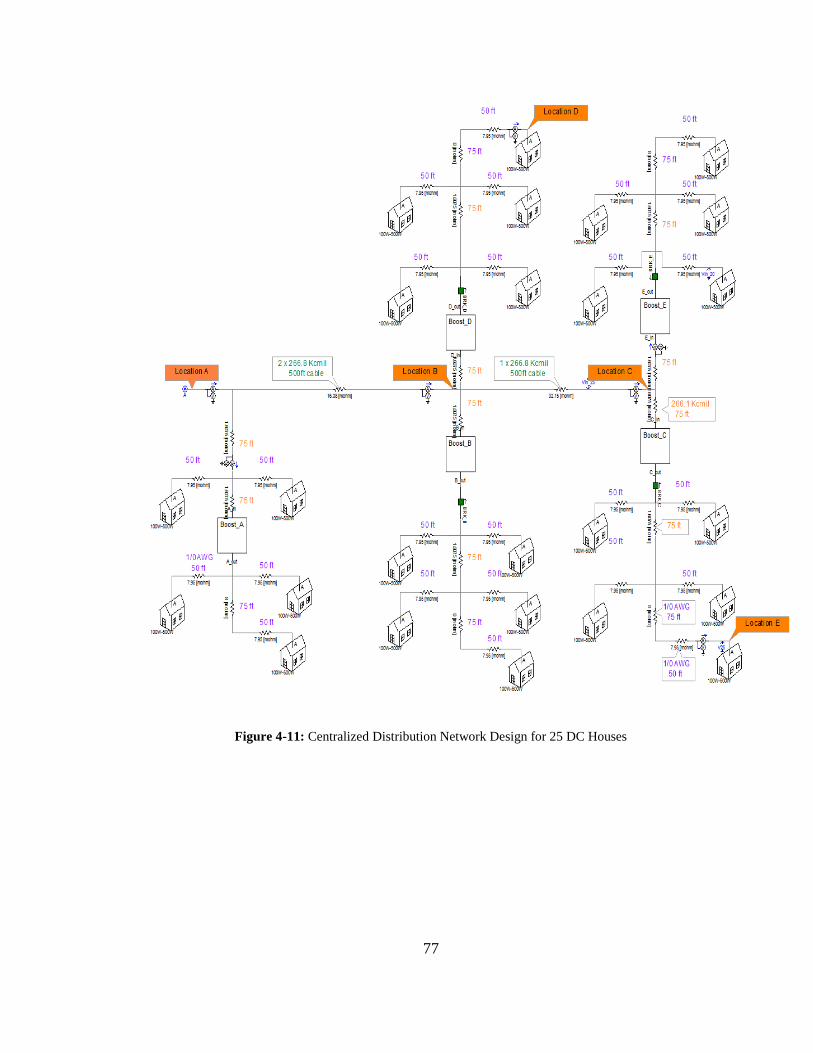
77
Figure 4-11: Centralized Distribution Network Design for 25 DC Houses
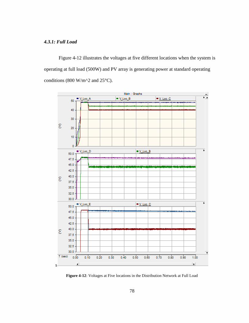
78
4.3.1: Full Load
Figure 4-12 illustrates the voltages at five different locations when the system is
operating at full load (500W) and PV array is generating power at standard operating
conditions (800 W/m^2 and 25°C).
s
Figure 4-12: Voltages at Five locations in the Distribution Network at Full Load

79
The top graph (Figure 4-12) shows voltages across the main distribution
conductor. The voltage at location A (which is at same location as source) is averaging
around 48.7V. Location B is 500ft away from the main source. Two Waxwing (2×266.1
kcmil) conductors are used to transmit power across this distance. There is a 4V drop
across the Waxwing conductors due to its DC resistance, and the voltage at location B is
44V. Location C is at 500ft from location B and only one Waxwing (1×266.1 kcmil) is
used to transmit power across this distance because it carries only about half as much
current as the first conductors. Moreover, the voltage at location C is around 40V. This
portrays that these voltage drops are dependent upon three variables: distance, load, and
cable resistance.
The middle graph (Figure 4-12) depicts the voltage difference between Location
B (beginning of Feeder D) and the voltage supplied to the individual house at location D
(at the end of the Feeder D). The voltage from location B is boosted back to 48V by the
Boost Converter and distributed to the DC Houses in Feeder D. Similarly, voltage at
location C is boosted back to 48V and is distributed to the DC Houses in Feeder C, as
depicted in bottom graph of Figure 4-12.
Figure 4-13 shows the current in the main conductors and into the two individual
houses at Locations D and E. As anticipated location A conducts the maximum current of
about 310A, followed by location B current of about 260A, and then the current at
location C is about 130A. The individual houses are supplied with 10.4A, which proves
that they are consuming about 500W when operating at 48V. The current ripple
significantly depends on the inductor value of the Buck Converter (on the source side).

80
The inductor with lower value closer to the boundary conduction mode leads to higher
ripple in the system.
Figure 4-13: Current at Five Locations in the Distribution Network at Full Load
Figure 4-14 depicts the power flow in the distribution network. The bottom graph
(Figure 4-14) validates that the individual houses are consuming about 500W. In the
steady state (around .2 seconds), the source is supplying approximately 14.6 kW and all
of the houses combined are consuming little over 12.5 kW. So, approximately 2 kW of
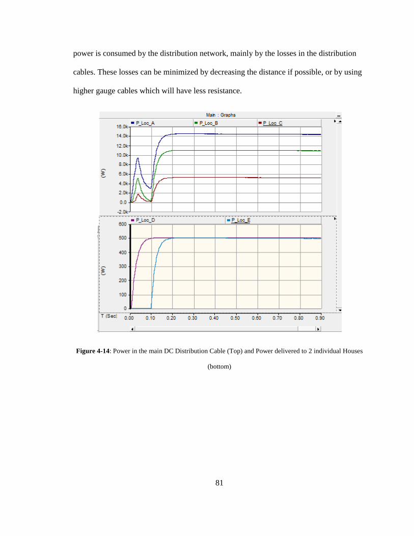
81
power is consumed by the distribution network, mainly by the losses in the distribution
cables. These losses can be minimized by decreasing the distance if possible, or by using
higher gauge cables which will have less resistance.
Figure 4-14: Power in the main DC Distribution Cable (Top) and Power delivered to 2 individual Houses
(bottom)

82
4.3.2: Varying Load
In the second simulation test, the house load is incremented from 100W to 500W
in steps of 50W every 0.1 seconds. Figure 4-15 illustrates voltage measurements of the
network as the load is varied. Higher load yields higher current in the system which
contributes to higher voltage drops across the distribution conductors (Vdrop = I*Rcable).
However, the dynamic response of the Boost Converters keeps the distributed house
voltage close to 48V (± 0.5V) consistently, as depicted on the bottom two graphs of
Figure 4-15.
Figure 4-15: Voltage Measurements as Load is incremented from 100W to 500W in steps of 50W

83
The current flow in the system increases in accordance with the load, as depicted
in Figure 4-16. The current ripple increases as the amount of current in the system
increases.
Figure 4-16: Current Measurements at Five Locations as load is incremented from 100W to 500W in steps
of 50W
Figure 4-17 depicts the power flow increases with the increasing load. The losses
in the distribution network increase as well with the increasing current (Ploss = I2*Rcable).
Next, the number of houses operating at full load is incremented from 5 to 25 in step of 5.

84
Figure 4-17: Power measurements at 5 different locations as load incremented from 100W to 500W in
steps of 50W
4.3.3: Varying Number of Houses Operating
Figure 4-18 shows voltage stability in the network as the number of houses
consuming power at full load is increased from 5 to 25 in steps of 5. Table 4-7
summarizes the voltage measurements at the five locations in the system. The current in
the system increases in accordance with the number of houses consuming power, which
leads to the voltage drops at locations B and C. These voltage drops are compensated by
the Boost Converters and the voltage at locations D and E is kept stable at 48V.

85
Similarly, Figure 4-19 and 4-20 show the current and power flow in the system with five
houses added to the network every 0.2 seconds.
Figure 4-18: Voltage Measurements at Five Locations as Number of Houses is incremented
Table 4-7: Distribution Network Voltages with 5 to 25 Houses at 500W
Time (sec) Houses Location A
(V)
Location B
(V)
Location C
(V)
Location D
(V)
Location E
(V)
0.1 5 48.7 48.2 48.2 48.4 48.3
0.2 10 48.5 47.1 47.5 48.2 48.2
0.4 15 48.2 46.2 44.5 48.1 48
0.6 20 48 45.2 43.1 47.9 47.9
0.8 25 47.8 44.1 40.1 47.8 47.7
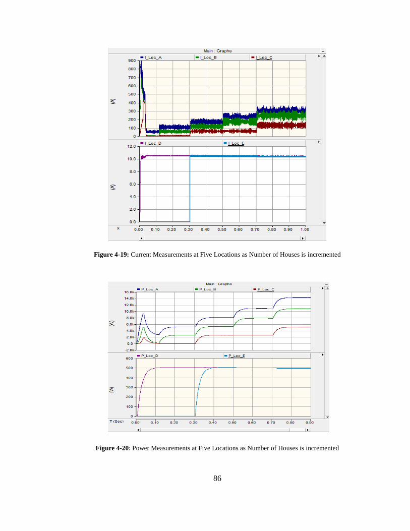
86
Figure 4-19: Current Measurements at Five Locations as Number of Houses is incremented
Figure 4-20: Power Measurements at Five Locations as Number of Houses is incremented

87
4.4: PV Charging the Battery and Supplying the Load
Figure 4-21 illustrates the peak sun hour power generation capacity of the PV
source. During the peak sun hours, the PV array produces more power than the load
demands and this excess power is used to charge the battery bank.
Figure 4-21: Battery Storage during Peak Sun Hours (dark yellow) and Battery Supplying Load (green)
For night time operation (approximately14 hours of non-generation period),
battery bank will require approximately 48 kWh of energy in order to supply the DC
houses, which will consume 100W-150W each. A test case is run where the excess power
from the PV array during peak sun hours is used to charge the battery bank. Figure 4-22
shows that 6.8 kW of energy is supplied to the battery and at this rate, 7 peak sun hours
Pow
er

88
will provide the battery bank with enough energy to last through the night time. Figure 4-
23 illustrates the battery current and voltage.
Figure 4-22: Power Supplied to the Battery from PV Array
Figure 4-23: Battery Current (blue) and Voltage (green)
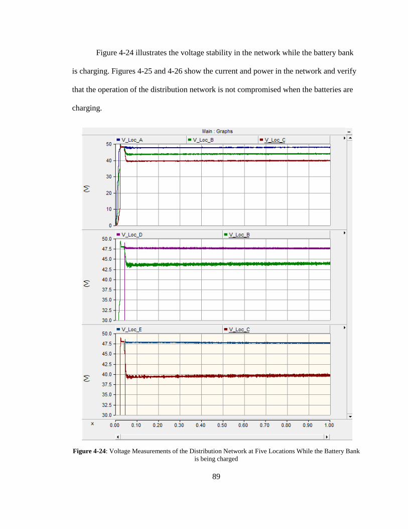
89
Figure 4-24 illustrates the voltage stability in the network while the battery bank
is charging. Figures 4-25 and 4-26 show the current and power in the network and verify
that the operation of the distribution network is not compromised when the batteries are
charging.
Figure 4-24: Voltage Measurements of the Distribution Network at Five Locations While the Battery Bank
is being charged
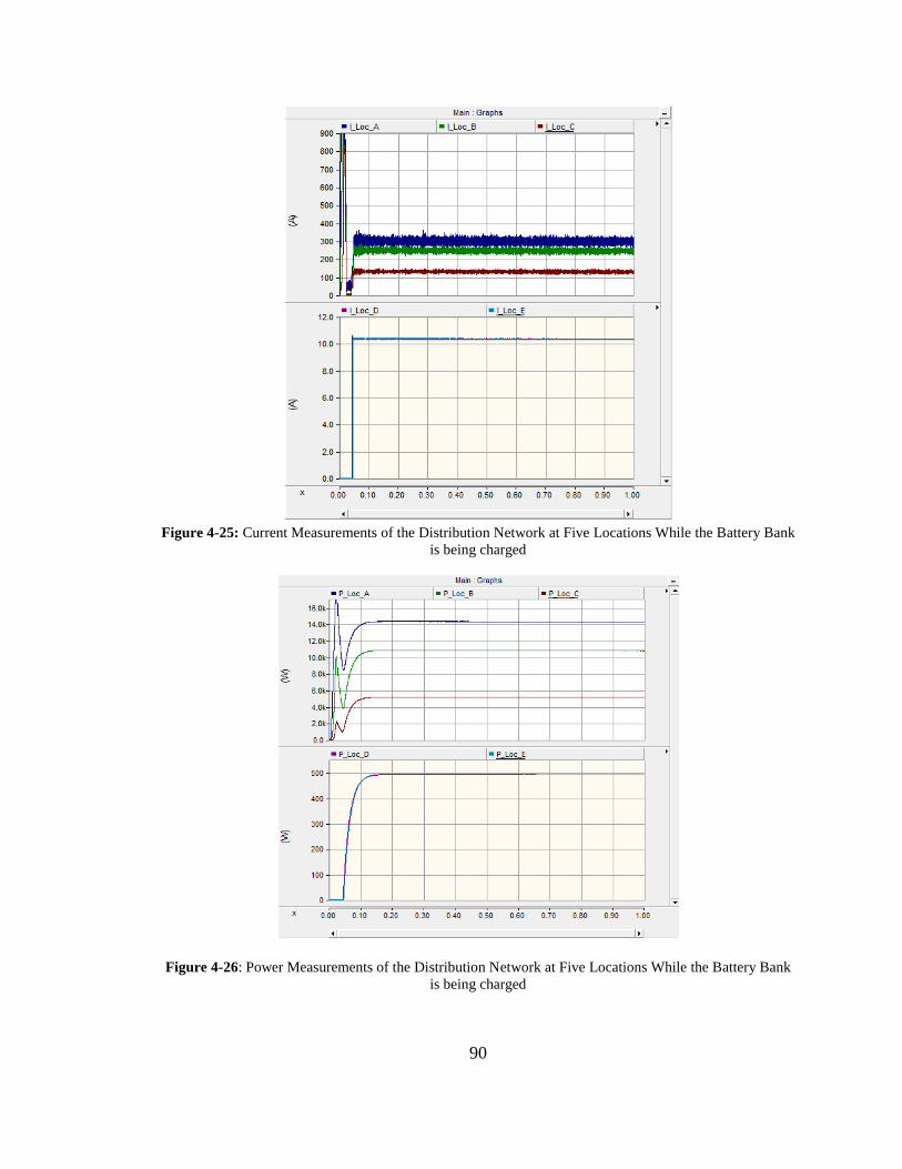
90
Figure 4-25: Current Measurements of the Distribution Network at Five Locations While the Battery Bank
is being charged
Figure 4-26: Power Measurements of the Distribution Network at Five Locations While the Battery Bank
is being charged
91
4.5: Battery Bank Supplying the Load
4.5.1: Varying Load
Similar to the test case in section 4.3.2, the load is varied from 100W to 500W
with steps of 50W every 0.1 seconds; however, the load is supplied from the battery bank
instead of PV (emulating night time or cloudy weather conditions). The input parameters
of the battery bank are shown in Figure 3-38 (previous chapter). Figure 4-27 shows the
voltage stability in the network as the load is increased. The DC bus voltage is regulated
at 48V by the Boost Converter, which is cascaded with the battery bank (Figure 4-1). The
voltage for the DC Houses (Locations D and E) is observed at 48V. Figures 4-28 and 4-
29 show the current and power flow in the network with the increasing load.
Furthermore, Figure 4-30 shows the decreasing SOC (state of charge) of the battery with
time, which shows that power is being drawn from the battery. This test case verifies that
the battery bank is able to provide smooth power to the DC Houses during non-
generation periods.

92
Figure 4-27: Voltage Measurements of Distribution Network at Five Locations as Load is increased from
100W to 500W in steps of 50W (Powered from Battery)

93
Figure 4-28: Current Measurements of Distribution Network at Five Locations as Load is increased from
100W to 500W in steps of 50W (Powered from Battery)

94
Figure 4-29: Power Measurements of Distribution Network at Five Locations as Load is increased from
100W to 500W in steps of 50W (Powered from Battery)
Figure 4-30: Battery Bank State of Charge (SOC)
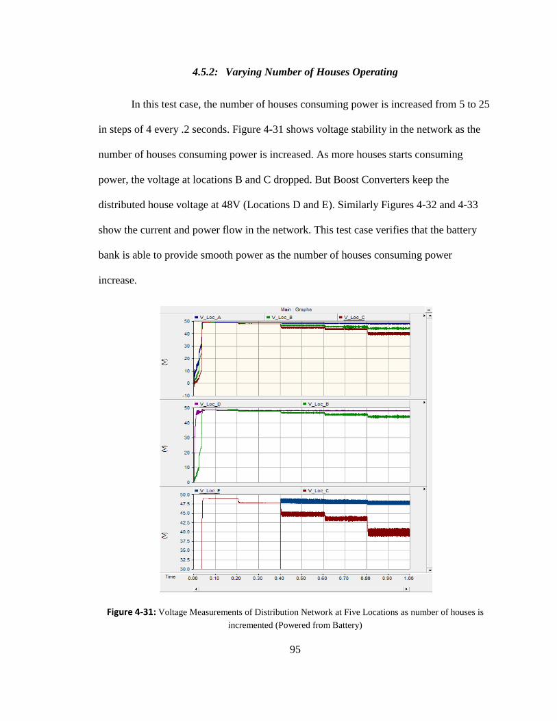
95
4.5.2: Varying Number of Houses Operating
In this test case, the number of houses consuming power is increased from 5 to 25
in steps of 4 every .2 seconds. Figure 4-31 shows voltage stability in the network as the
number of houses consuming power is increased. As more houses starts consuming
power, the voltage at locations B and C dropped. But Boost Converters keep the
distributed house voltage at 48V (Locations D and E). Similarly Figures 4-32 and 4-33
show the current and power flow in the network. This test case verifies that the battery
bank is able to provide smooth power as the number of houses consuming power
increase.
Figure 4-31: Voltage Measurements of Distribution Network at Five Locations as number of houses is
incremented (Powered from Battery)

96
Figure 4-32: Current Measurements of Distribution Network at Five Locations as number of houses is
incremented (Powered from Battery)
Figure 4-33: Power Measurements of Distribution Network at Five Locations as number of houses is
incremented (Powered from Battery)

97
4.6: System Cost Analysis
The major factor driving the growth of the renewable energy sources such as
photovoltaic is their competitive cost, which has been decreasing for the past two
decades. The DC distribution method is chosen for our system because it is more efficient
and requires fewer components than an AC distribution method. In the following
sections, a DC vs. AC distribution cost analysis is performed for a system that could
range from 10 kW to 100 kW.
4.6.1: PV Array and MPPT Charge Controller Cost
The adequate sizing of PV array is important to prolong the life of the system
components, house appliances, and battery bank. PV array sizing is based on the lowest
insolation month (critical month) of the place where system will be implemented. Since
the DC house project is to be mainly used in developing countries, the insolation data of
Jakarta, Indonesia, will provide for system sizing. From the data in Figure 4-34, it is clear
that the lowest insolation month in Jakarta is January when the average insolation is 4.25
kWh/m2/day.
Figure 4-34: Jakarta Indonesia Monthly Insolation [36]
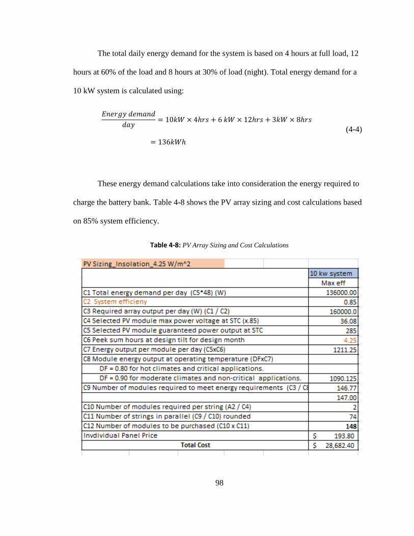
98
The total daily energy demand for the system is based on 4 hours at full load, 12
hours at 60% of the load and 8 hours at 30% of load (night). Total energy demand for a
10 kW system is calculated using:
𝐸𝑛𝑒𝑟𝑔𝑦 𝑑𝑒𝑚𝑎𝑛𝑑
𝑑𝑎𝑦= 10𝑘𝑊 × 4ℎ𝑟𝑠 + 6 𝑘𝑊 × 12ℎ𝑟𝑠 + 3𝑘𝑊 × 8ℎ𝑟𝑠
= 136𝑘𝑊ℎ
(4-4)
These energy demand calculations take into consideration the energy required to
charge the battery bank. Table 4-8 shows the PV array sizing and cost calculations based
on 85% system efficiency.
Table 4-8: PV Array Sizing and Cost Calculations

99
JAP6- 285W solar module is selected for the system due to its competitive price
per watt (Appendix A). Table 4-9 summarizes the cost for a system ranging from 10 kW
to 100 kW with 85% and 75% system efficiencies. The data from the table are plotted in
Figure 4-35. The plot shows that improving the system efficiency is significant in
reducing the high initial cost for a PV system.
Table 4-9: Summary of PV Cost for 85% and 75% System Efficiency
System kW 85% eff 75% eff
10 $ 28,682.40 $ 32,558.40
20 $ 56,977.20 $ 64,729.20
30 $ 85,659.60 $ 96,900.00
40 $ 113,954.40 $ 129,070.80
50 $ 142,249.20 $ 161,241.60
60 $ 170,931.60 $ 193,800.00
70 $ 199,226.40 $ 225,970.80
80 $ 227,908.80 $ 258,141.60
90 $ 256,203.60 $ 290,312.40
100 $ 284,498.40 $ 322,483.20
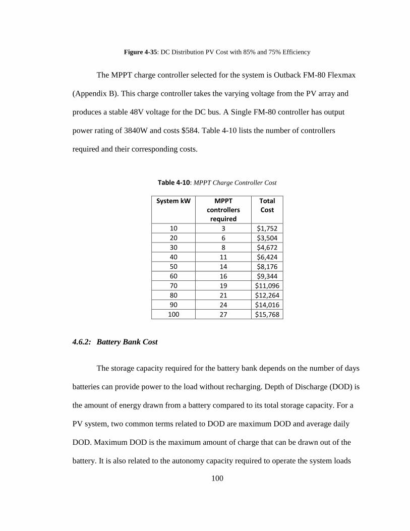
100
Figure 4-35: DC Distribution PV Cost with 85% and 75% Efficiency
The MPPT charge controller selected for the system is Outback FM-80 Flexmax
(Appendix B). This charge controller takes the varying voltage from the PV array and
produces a stable 48V voltage for the DC bus. A Single FM-80 controller has output
power rating of 3840W and costs $584. Table 4-10 lists the number of controllers
required and their corresponding costs.
Table 4-10: MPPT Charge Controller Cost
System kW MPPT controllers
required
Total Cost
10 3 $1,752
20 6 $3,504
30 8 $4,672
40 11 $6,424
50 14 $8,176
60 16 $9,344
70 19 $11,096
80 21 $12,264
90 24 $14,016
100 27 $15,768
4.6.2: Battery Bank Cost
The storage capacity required for the battery bank depends on the number of days
batteries can provide power to the load without recharging. Depth of Discharge (DOD) is
the amount of energy drawn from a battery compared to its total storage capacity. For a
PV system, two common terms related to DOD are maximum DOD and average daily
DOD. Maximum DOD is the maximum amount of charge that can be drawn out of the
battery. It is also related to the autonomy capacity required to operate the system loads

101
for given number of days with no generation from PV. A system designed with very low
DOD will have most of the battery energy available to the load but with a trade-off for
longer battery life. The average daily DOD is the amount of energy drawn from battery’s
full capacity with the average daily load profile. A system designed for longer autonomy
periods (more capacity) will have lower average daily DOD. For this system, DOD of
80% is selected, which is typical for isolated PV storage systems. For the battery bank,
Trojan T105-RE Flooded lead-acid battery is selected (Appendix C), which has 225A of
capacity with 6V terminal voltage. Table 4-11 shows the calculations for the number of
batteries required for a 10 kW to 100 kW system and their corresponding costs, assuming
two days of autonomy storage are required.

102
Table 4-11: Battery Bank Sizing for 2 Days of Autonomy Storage

103
Furthermore, Table 4-12 summarizes the variations in the battery cost as the size
of the system and number of days are varied. Data shows that the battery cost is
significantly higher as the autonomy storage days are increased. This is because battery
prices have not dropped like the PV module prices. Additionally Figure 4-36 shows a 3D
graph of the battery cost.
Table 4-12: Battery Cost Varied with System Size and Storage Capacity
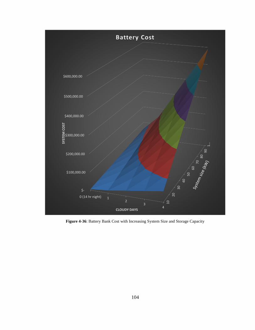
104
Figure 4-36: Battery Bank Cost with Increasing System Size and Storage Capacity
10
20
30
40
50
60
70
80
90
1…
$-
$100,000.00
$200,000.00
$300,000.00
$400,000.00
$500,000.00
$600,000.00
0 (14 hr night) 12
34
SYST
EM C
OST
CLOUDY DAYS
Battery Cost

105
4.6.3: Distribution Cost
The selection criteria for the distribution conductors is their DC resistance and
prices. For the main distribution lines, ASCR Waxing (266.8 kcmil) conductor is chosen
and Raven (1/0 AWG) is selected to connect single house to the main conductors. Table
4-13 shows the calculated cost for the 10 kW. Table 4-14 shows the total distribution
cost for the wiring and Boost Converter (Appendix D) for a 10 kw -100 kW system.
Table 4-13: Distribution Wiring Cost for a 10 kW System.
Table 4-14: Distribution Wiring and Boost Converter Cost
Table 4-15 shows the total cost of the Centralized DC Distribution System for the
DC House. The battery cost is for the best case scenario, which is only accounting for

106
enough storage for the night-time operations. This cost will multiply if more autonomy
storage capacity is desired.
Table 4-15: Total DC System Cost
4.6.4: AC System Cost
In order to justify the DC distribution method a comparison study was prepared
for the AC distribution cost. The AC system is less efficient because of the extra
conversion stages, which are not required in the DC distribution. The AC system requires
an inverter to convert DC to AC on the source side. SMA Sunny Boy 10000TLUS-10 10
kW inverter is selected (Appendix E). The common AC distribution voltage is 12.4 kV,
which means transformers are required to step-up the voltage at the source end and step-
down on the house side to supply the house at 120V. The transformer selected for the AC
network is ABB Single phase overhead distribution transformer (Appendix F). Table 4-
16 details the cost analysis for the AC system. The PV cost for the AC system is
calculated assuming system efficiency of 75%. The cost for MPPT charge controller and

107
battery bank remains unchanged from the DC system. But the wiring cost is half of the
DC system because smaller cable conductors are needed for the high voltage distribution.
Table 4-16: Total AC System Cost
Figure 4-36 graphs the cost difference between the DC and AC distributions. In
this figure, the DC system is assumed to be at 85% efficiency and AC system to be at
75% efficiency. The cost difference between the two distribution methods grows larger as
their efficiency gap increases.
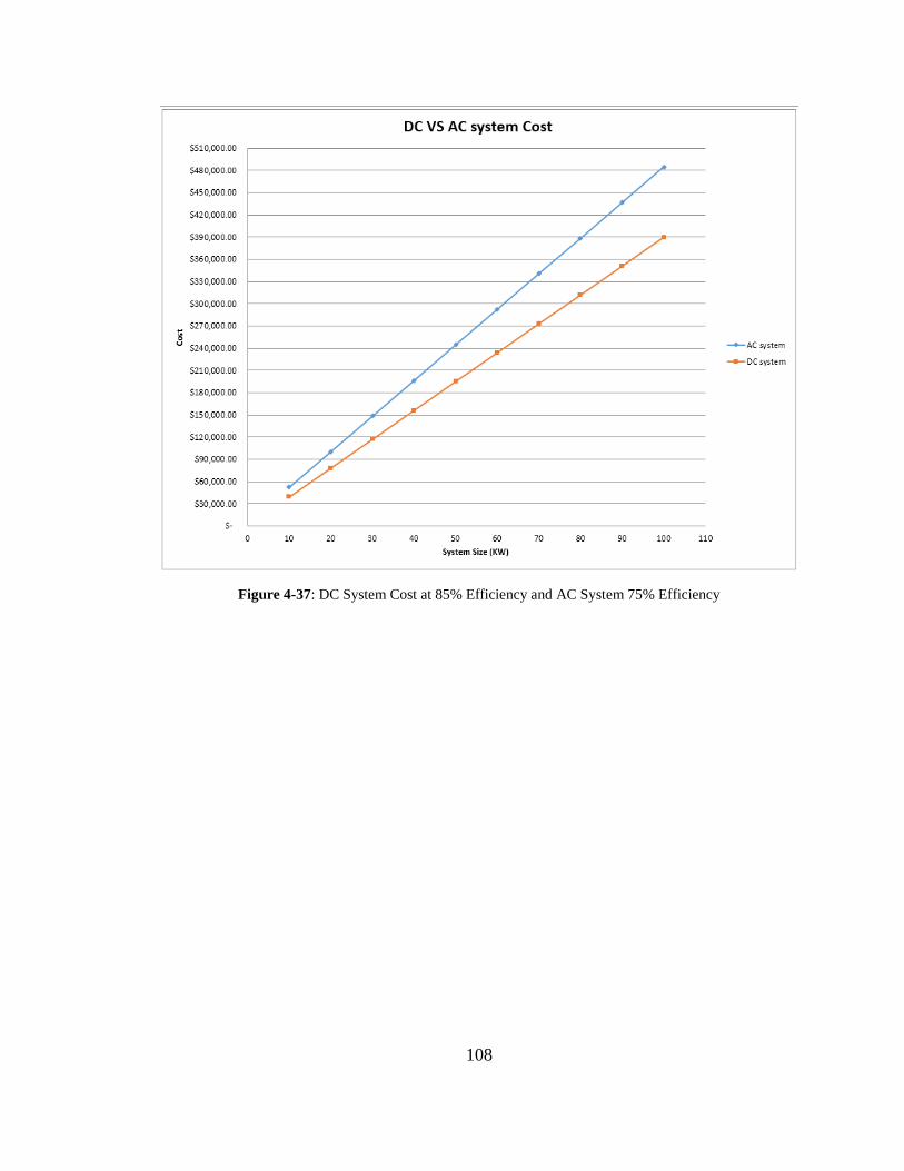
108
Figure 4-37: DC System Cost at 85% Efficiency and AC System 75% Efficiency
109
Chapter 5
Conclusion and Future Work
5.1: Summary and Conclusion
This thesis focuses on the design, modeling, simulation, and performance
evaluation of a DC House centralized distribution network. The complete system was
modeled in PSCAD. The simulation results proved that the design meets the DC bus
voltage stability requirements under different operating conditions. Different variations in
the weather patterns can affect the PV generation. Simulation results further verified that
the MPPT controller responds to the different weather patterns accordingly. The PV
source is kept at its maximum power generating point by the MPPT controller and the
buck converter by regulating the DC bus voltage at 48V. The PV source is able to supply
the load and charge the battery bank during the peak sun hours without having any
voltage instability at the DC bus. In addition, during night-time operation the battery
bank is able to supply the load at stable 48V.
The distribution network layout was modeled with 25 houses (Figure 4-11). The
voltage drops in the network were caused by the resistive losses of the conductors (Figure
4-12). The boost converters in the distribution network kept the voltage supplied to the
load at 48V (Figure 4-12).
110
The efficiency of the power converters at the source side was observed to range
from 88.85% to 93.47%, based on the load demand (Table 4-6). On the other hand, the
efficiency of the distribution network depends on the distance that the network has to
cover and the conductor type utilized. The losses in the distribution network can be
minimized by choosing higher gauge conductors and reducing the distance if possible.
DC vs. AC cost analysis showed that the isolated DC centralized distribution
system is more cost effective of the two systems. The AC distribution is burdened by the
extra conversion stages which require extra components and reduce efficiency. Other
factors, such as power factor correction and frequency stability, are not relevant in the
DC system. The factors together provide for a simple, efficient and cost effective system.
5.2: Future Work
For simplicity, this study only included PV renewable source as part of the system
but the concept of the DC House includes many other renewable sources such as: wind,
hydro, human-powered generator. In the future work these sources can also be integrated
into a larger simulation model.
More thorough study can also be performed on the performance of the battery bank
by looking at the charge, discharge cycle and the battery health over its life. A battery
bank is a heart of isolated this isolated distribution system therefore more thorough study
will help improve the performance of the whole system.
This system is at a low voltage distribution which leads to high currents in the
network. To ensure reliable operation of the distribution network, it is important to have a

111
good protection system. Future simulations could create a protection scheme for the
system by integrating current interruption devices in case of faults, relays and proper
grounding schemes. Future study should also be conducted to determine the most
optimum distribution voltage for the DC house network.
Overall this thesis produced a basic simulation model for the centralized DC
house distribution system which will be further built upon in the future.

112
References
[1] International Energy Agency, “CO2 Emissions From Fuel Combustion
Highlights," IEA, Paris, 2012 .
[2] McaCarley, Art “ The Carbon Cycle and Global Warming.” Cal Poly San Luis
Obispo University. EE 563 Seminar. 15 March 2013
[3] Novus Light Technologies Today, "EPIC Release Photovoltaic Industry Report,"
2012. [Online]. Available: http://www.novuslight.com/epic-releases-
photovoltaic-industry-report_N182.html. [Accessed 2013].
[4] K. Liang, "Design of DC Light Bulb for teh DC House Project," California
Polytechnic State University, San Luis Obispo, 2012.
[5] J. Kuderna, "RV Basics: 12-Volt DC Systems," RVtravel, [Online]. Available:
http://www.rvtravel.com/publish/12-Volt_DC_Systems.shtml. [Accessed 2013].
[6] All About Circuits, "Skin Effect," [Online]. Available:
http://www.allaboutcircuits.com/vol_2/chpt_3/6.html. [Accessed 2013].
[7] J. Parmar, "What is Corona Effect," 23 March 2011. [Online]. Available:
http://electricalnotes.wordpress.com/2011/03/23/what-is-corona-effect/.
[8] J. Chaidez, "DC House Modeling and System Design," California Polytechnic
State University, San Luis Obispo, 2011.
[9] Crowfoot, J., "Design and Modeling of the Cal Poly DC House Power
Distribution System," California Polytechnic State University,, San Luis Obispo,
2011.
[10] Pratt, A.; Kumar, P.; Aldridge, T.V., "Evaluation of 400V DC distribution in
telco and data centers to improve energy efficiency," Telecommunications
Energy Conference, 2007. INTELEC 2007. 29th International
[11] Gab-Su Seo; Jongbok Baek; Kyusik Choi; Hyunsu Bae; Bohyung Cho,
"Modeling and analysis of DC distribution systems," Power Electronics and
ECCE Asia (ICPE & ECCE), 2011 IEEE 8th International Conference

113
[12] Lim, E.; Liu, S., "Wind Power Generator Design for the DC House Project,"
California Polytechnic State Univeristy, San Luis Obispo, 2011.
[13] Kwan, D.; Krug, M., "Hydro-Electric Generation System for the DC House
Project," California Polytechnic State University, San Luis Obispo, 2011.
[14] Hayes, B.; Goguely, L., "Bicycle Power Generation Design for DC house: Off
Grid Energy Solutions," California Polytechnic State UNiversity, San Luis
Obispo, 2011.
[15] Tonkoski, R.; Turcotte, D.; EL-Fouly, T. H M, "Impact of High PV
Penetration on Voltage Profiles in Residential
Neighborhoods," Sustainable Energy, IEEE Transactions
[16] C. K. T. Wong, "A Multiple-Input Single-Output DC-DC Converter for the DC
House Project," California Polytechnic State University, San Luis Obispo, 2011.
[17] O. Jong, "Multiple Input Single Output (MISO) DC-DC Converter For the DC
House Project," California Polytechnic State University, San Luis Obispo, 2012.
[18] A. Ma, "Modling and Analysis Of a Photovoltaic System with a Distributed
Energy Storage System," California Polytechnic State University,, San Luis
Obispo, 2012.
[19] S. Jiang, "Battery Component in PSCAD/EMTDC," Manitoba HVDC Research
Centre, Winnipeg, 2012.
[20] Taufik, "The DC House Project Promoting Sustainable Innovations in
Renewable Energy Technology," California Polytechnic State University, San
Luis Obispo.
[21] Rajapakse, A.D.; Muthumuni, D., "Simulation tools for photovoltaic
system grid integration studies," Electrical Power & Energy Conference
(EPEC), 2009 IEEE
[22] P. Mars, "Using a Small Solar Cell and a Supercapacitor in a Wireless Sensor,"
Sensors, 1 July 2010. [Online]. Available:
http://www.sensorsmag.com/networking-communications/energy-
harvesting/using-a-small-solar-cell-and-a-supercapacitor-a-wireless-sen-7310.
[Accessed 2013].
[23] J. Dunlop, "Batteries and Charge Charge Control in Stand-Alone Photovoltaic
Systems Fundamental and Application," Florida Solar Energy Center, 1997.
[24] Battery University, "Comparison Table of Secondary Batteries," [Online].
Available:

114
http://batteryuniversity.com/index.php/learn/article/secondary_batteries.
[Accessed 2013].
[25] E. Jones, "Lead Acid Batteries in Critical Applications Flooded vs. VRLA,"
C&D Technologies, Inc,.
[26] Hund, T, Dunlop, J. and Farhi, B., "Test Results from the PV Battery Cycle-Life
Test Procedure," Photovoltaic System Applications Department Sandia National
Laboratories, Albuquerque, NM.
[27] Wholesale Solar, "Battery Bank Sizing Worksheet," [Online]. Available:
http://www.wholesalesolar.com/battery_sizing.html. [Accessed 2013].
[28] Kadri,R; Andrei, H.; Gaubert, J.; Ivanovici,T.:, "Modeling of the photovoltaic
cell circuit parameters for optimum connection model and real-time emulator
with partial shadow conditions," Elsevier, 2011.
[29] Veerachary, M., "Maximum power point tracking parameter selection
for higher order converters used in photovoltaic applications," Power
Systems, 2009. ICPS '09. International Conference
[30] Esram, T.; Chapman, P.L., "Comparison of Photovoltaic Array
Maximum Power Point Tracking Techniques," Energy Conversion,
IEEE Transactions
[31] L. Guo, "PSCAD Simulation in a Power Electronics Application Course,"
Department of Technology Northern Illinois University, 2008.
[32] Taufik, “Introduction to Power Electronics”, Notes, San Luis Obispo, 2011.
[33] Wikipedia, "Boost Converter," [Online]. Available:
http://en.wikipedia.org/wiki/Boost_converter. [Accessed 2013].
[34] N. Rumzi, "Buck Converter," University Teknologi Malaysia (UTM), [Online].
Available: http://encon.fke.utm.my/nikd/SEM4413/AnalysisConverter-buck.pdf.
[Accessed 2013].
[35] Coelho, R. F; Martins, D. C, "An Optimized Maximum Power Point Tracking
Method Based on PV Surface Temperature Measurement," Federal University of
Santa Catarina, Flrianopolis, Brazil.
[36] NASA, "Jakarta, Indonesia-Insolation," Gaisma, [Online]. Available:
http://www.gaisma.com/en/location/jakarta.html. [Accessed 2013].
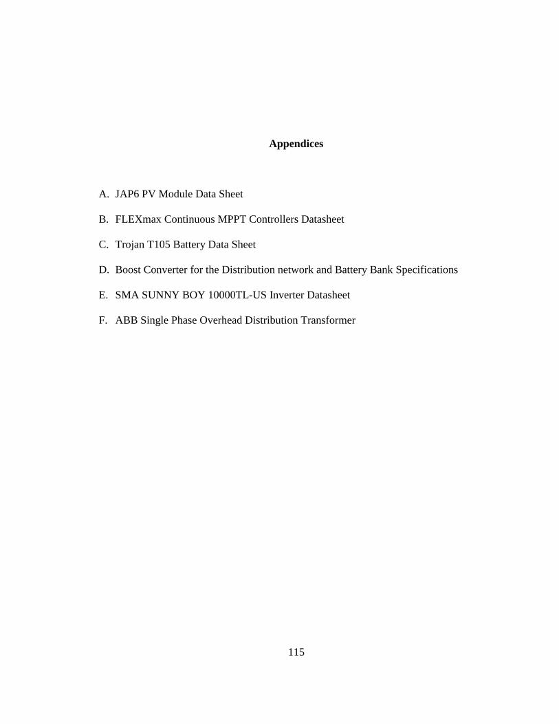
115
Appendices
A. JAP6 PV Module Data Sheet
B. FLEXmax Continuous MPPT Controllers Datasheet
C. Trojan T105 Battery Data Sheet
D. Boost Converter for the Distribution network and Battery Bank Specifications
E. SMA SUNNY BOY 10000TL-US Inverter Datasheet
F. ABB Single Phase Overhead Distribution Transformer

116
Appendix A
JAP6 PV Module Data Sheet
Figure A-1: JAP6 PV Module Datasheet Page 1

117
Figure A-2: JAP6 PV Module Datasheet Page 2
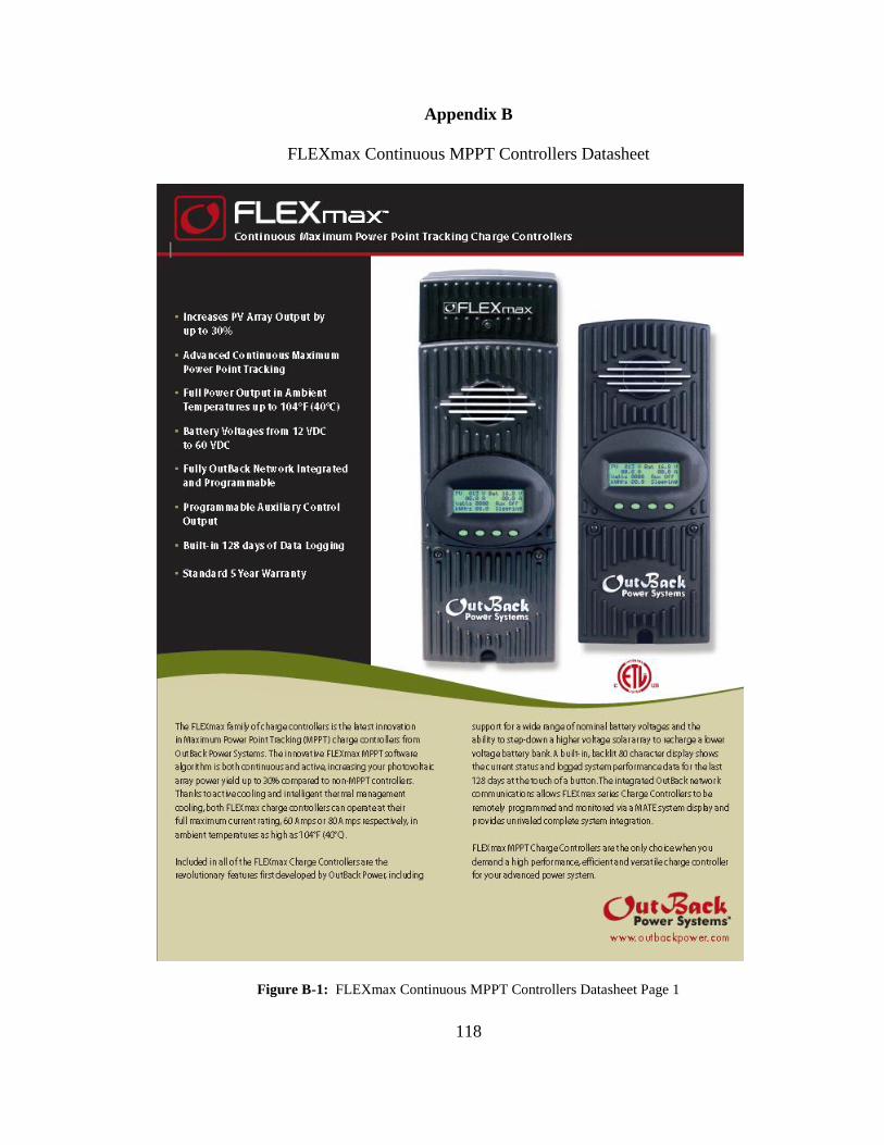
118
Appendix B
FLEXmax Continuous MPPT Controllers Datasheet
Figure B-1: FLEXmax Continuous MPPT Controllers Datasheet Page 1
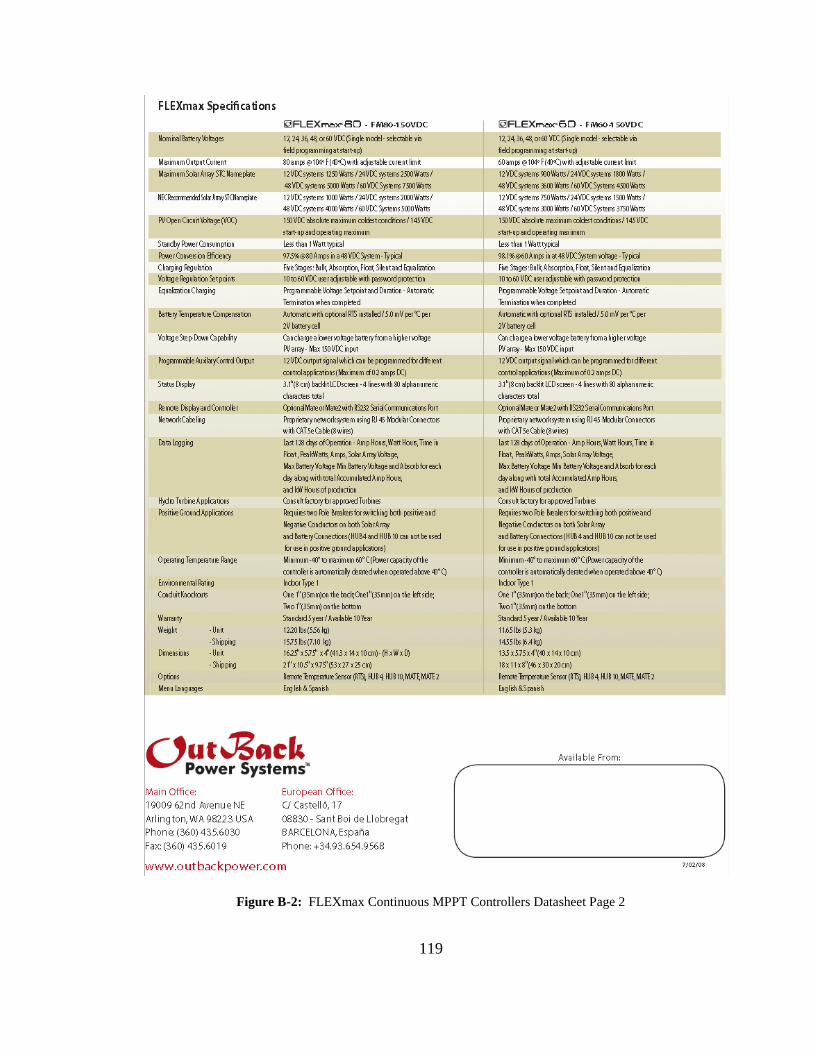
119
Figure B-2: FLEXmax Continuous MPPT Controllers Datasheet Page 2
120
Appendix C
Trojan T105 Battery Data Sheet
Figure C-1: Trojan T105 Battery Data Sheet Page 1

121
Figure C-2: Trojan T105 Battery Data Sheet Page 2
122
Appendix D
Boost Converter for the Distribution network and Battery Bank Specifications
Figure D-1: Boost Converter for the Distribution network and Battery Bank description

123
Appendix E
SMA SUNNY BOY 10000TL-US Inverter Datasheet
Figure E-1: SMA SUNNY BOY 10000TL-US Inverter Datasheet Page 1

124
Figure E-2: SMA SUNNY BOY 10000TL-US Inverter Datasheet Page 2

125
Appendix F
ABB Single Phase Overhead Distribution Transformer
Figure F-1: ABB Single Phase Overhead Distribution Transformer Datasheet Page 1

126
Figure F-2: ABB Single Phase Overhead Distribution Transformer Datasheet Page 2

127
Figure F-3: ABB Single Phase Overhead Distribution Transformer Datasheet Page 3