non-commercial joint stock company almaty university of

ANALYSIS OF ELECTRICAL CIRCUITS AND ELECTRIC FIELD

THEORY OF NONLINEAR CIRCUITS AND ELECTRIC FIELD

Methodological guidelines and assignments for laboratory works

for the 5B071800 – Electrical power engineering baccalaureate specialty students

Almaty 2017

Non-commercial

joint stock

company

ALMATY

UNIVERSITY OF

POWER

ENGINEERING &

TELECOMMUNICATIONS

Department of Theoretical

electrical engineering

2

AUTHORS: A. S. Baimaganov, S. J. Kreslina. Analysis of electrical circuits

and electric field. Theory of nonlinear circuits and electric field. Methodological

guidelines and assignments for laboratory works for the 5B071800 – Electrical

power engineering baccalaureate specialty students. – Almaty: AUPET, 2017. – 27

p.

Methodological guidelines and assignments for preparing, carrying out and

design of laboratory works on “Analysis of electrical circuits and electric field” and

“Theory of nonlinear circuits and electric field” disciplines are provides.

Each laboratory work includes the following sections: an objective of the

work, preparation for a laboratory work, procedure of carrying out the work, pro-

cessing the results of experiments and methodological guidelines.

Methodological guidelines and assignments are intended for second-year stu-

dents, who are educated in English language on the 5B071800 – “Electrical power

engineering” baccalaureate specialty.

13 illustrations, 6 tables, 9 items of references.

Reviewer: PhD B. I. Tuzelbayev

It is printed according to the publishing plan of non-commercial JSC “Almaty

university of power engineering & telecommunications” for 2017 y.

© NJSC “Almaty university of power engineering & telecommunications”, 2017 y.

3

2017 y. publishing plan, 33 position

Aliaskar Baimaganov

Svetlana Kreslina

ANALYSIS OF ELECTRICAL CIRCUITS AND ELECTRIC FIELD

THEORY OF NONLINEAR CIRCUITS AND ELECTRIC FIELD

Methodological guidelines and assignments for laboratory works

for the 5B071800 – Electrical power engineering baccalaureate specialty students

Editor Y. R. Gabdulina

Standard expert N. K. Moldabekova

Signed to publication _____________ Layout size 60×84 1/16

Printed 50 copies Printout paper № 1

Volume 1.7 edu.-pub. sheet Order ____ Price 850 tenge

Copying service

Non-commercial joint stock company

“Almaty university of power engineering & telecommunications”

126, Baitursinov Street, Almaty, 050013

4

Contents

Introduction ....................................................................................................... 5

Requirements for the registration of report on laboratory work ....................... 7

1 Laboratory work №1. Research of DC circuits with nonlinear elements ...... 9

2 Laboratory work №2. Research of electric circuits with valves .................. 11

3 Laboratory work №3. Research of the voltage ferroresonance

phenomenon .............................................................................................................. 14

4 Laboratory work №4. Research of the plane-parallel electrostatic field of a

two-wire line .............................................................................................................. 17

References ....................................................................................................... 27

5

Introduction

The laboratory research are of great importance for the quality of training and

formation of students’ creative thinking and engineering skills. The performance of

laboratory works allows students to apply theoretical principles in practical calcula-

tions in order to obtain skills of independent analysis of electrical circuits, which

ultimately contributes to the successful mastery of the discipline.

The manual contains a description of the laboratory works on the “Analysis

of electrical circuits and electric field” (AECEF) and “Theory of nonlinear circuits

and electric field” (TNCEF) elective disciplines for the 5B071800 – “Electrical

power engineering” baccalaureate specialty students.

Laboratory work is a complex of experimental and theoretical assignments in

the study of linear electric circuits of direct, single-phase and three-phase sinusoidal

current. All laboratory work is performed by the front way after the respective top-

ics in the lecture material is presented.

The practical implementation of the laboratory researches at the “Theoretical

electrical engineering” (TEE) department provides by using of the “UILS-2” – uni-

versal teaching and research laboratory workbenches. The UILS-2 workbench is

fixed on the table and is a metal box in which the active and passive units and a

patchbay for the assembly of electrical circuits to carry out the experiment are

mounted. The workbench also includes 29 external components (resistors, capaci-

tors and inductors) and a set of connecting leads with plugs.

Active blocks are located in the left side of the stand and consist of a block of

DC voltage sources and blocks of the single- and three-phase sinewave voltage

sources. Passive units are located in the right side of the stand and consist of a block

of a variable resistance and blocks of a variable inductance and a variable capaci-

tance. A patchbay is located at the center of the stand.

The DC voltage unit comprises:

- an adjustable DC stabilized voltage source with regulation range from 0.25

to 24 V;

- an unregulated DC voltage source with output voltage of about 20 V;

- “electronic switch” used to study transients.

Both DC voltage sources are provided with an electronic protection circuit

against short-circuits and overloads. The current of protection activation is 1 A.

AC unit is a functional generator with adjustable frequency and value of volt-

age of sinusoidal, rectangular and triangular shapes.

The unit is provided with an electronic protection circuit against short-circuits

and overloads. The current of protection activation is 1 A.

The three-phase voltage unit is a source of three-phase voltage of commercial

frequency f = 50 Hz. Source contains three electrically independent from each other

phases.

6

Each phase is equipped with an electronic protection against short-circuits

and overloads. The current of protection activation is 1 A.

The unit of variable resistors consists of three unregulated resistors R1, R2, R3

and an adjustable R4. Regulation of value of resistor R4 is performed in the range

from 0 to 999 Ω a stepwise in increments of 1 Ω by using three switches: the hun-

dreds (0 ... 9), the tens (0 ... 9) and the units (0 ... 9) Ω.

The unit of variable inductance includes three unregulated inductors L1, L2, L3

and an adjustable inductor L4. Regulation of inductance L4 can be adjusted between

0 and 99.9 mH in steps of 0.1 mH by using three switches: the tens (0 ... 9), the

units (0 ... 9) and the tenths (0 ... 9) mH.

The unit of variable capacitance consists of three unregulated capacitors C1,

C2, C3 and an adjustable C4. Regulation of capacitance C4 is carried out in the range

from 0 to 9.99μF in steps of 0.01 μF using three switches: the units (0 ... 9), the

tenths (0 ... 9) and the hundredths of (0 ... 9) μF.

On the front panel of the blocks are located: the light indicators (LEDs, light

indicators), the controls (knobs switches, toggle switches, and buttons) and meas-

urement devices.

A patchbay is a panel with 67 pairs connected with each other of jacks for

plugging and mounting the components of studied electrical circuits

The external elements are designed as the transparent plastic boxes, in which

there are plugs to connect and soldering inside the elements of electric circuits: R, L

and C.

It is necessary to switch the toggle switch “POWER” in “ON” position to turn

on the active unit, at the same time on front panel the “POWER LED” lights.

Measuring devices of the units are designed to display the value of current

and voltage of regulated sources. Regulation performed by means of potentiometer

handle.

The frequency is adjusted stepwise with 1 kHz step by a switch and smoothly

by a “FREQUENCY SMOOTHLY” potentiometer. When the potentiometer is at

the right position, the frequency of the output voltage corresponds to the value indi-

cated on the stepwise switch with an accuracy of ± 2%.

The voltage of each phase at the output of unit of the three-phase voltage

source can be adjusted stepwise from 0 to 30 V in increments 1 V via two switches:

tens (0 ... 3) and units (0 ... 9) of Volts.

In the event of a short circuit or an overload in the power supply units an

electronic protection is activated, and “PROTECTION” indicator lights. After re-

moving the causes of a short circuit or overload, it is necessary to return the power

supply unit in operating state by pressing “PROTECTION” button upon that the in-

dicator goes out.

7

Requirements for the registration of report on laboratory work

The assignment for the current laboratory work the student gets in advance on

the previous lesson, for one or two weeks earlier.

Each student prepares a report himself in order to carry out laboratory work,

acquainted with the purpose of work and with the basic theoretical principles used

in the experiment.

Before implementation of experimental part, the student is interviewed on the

preparation for a laboratory work. Then he shows the report prepared for the execu-

tion of laboratory work to the teacher and gets the admission to the work.

After executing the experimental part, the report is finalized: a comparison

between theory and experiment is carried out, the necessary graphs are plotted, an

analysis the results are carried out and conclusions on the work are made.

Each student defends the report on laboratory work individually at the current

or following laboratory classes, or at the consultations.

The report should contain the title page and the following sections:

- purpose of the work;

- basic theoretical principles and answers to questions of preparation for a

laboratory work;

- brief information about the experiment;

- the scheme of analyzed electric circuit;

- the formulas, and the results of theoretical calculations for specific modes

of the electric circuit;

- results of the study: tables, graphs, diagrams, numerical values of the cir-

cuit parameters, electric currents and voltages, etc.

- the conclusions of the work done.

See the template of the title page on the next page.

Reports should be performed only on a one side of white sheet or of lined pa-

per with size of A4 (210x297mm). The text should be written neatly. When writing

the text is permitted to use only generally accepted abbreviations or designations,

decrypted at the first mention.

Student is allowed to the next laboratory work if he has executed and defend-

ed a previous laboratory work.

8

Non-commercial Joint Stock Company

ALMATY UNIVERSITY OF POWER ENGINEERING & TELECOMMUNICATIONS

Department of Theoretical electrical engineering

R E P O R T

on laboratory work № ____

on the “Analysis of electrical circuits and electric field” discipline

or

on the “Theory of nonlinear circuits and electric field” discipline

__________________________________________________________________ (Title of the laboratory work)

__________________________________________________________________

5B071800 – “Electrical power engineering” baccalaureate specialty

Done by __________________________________ Group _____________ (Student’s Surname & Initials) (Academic group code)

Checked by ____________________________________________________ (Teacher’s academic degree, academic rank, Surname & Initials)

____________ ___________________ «____» ________________20___ y. (Score) (Teacher’s signature) (Date)

9

Almaty 20___ y.

1 Laboratory work №1. Research of DC circuits with nonlinear elements

The objective of the work is obtaining the skills of experimental research of

direct current circuits with nonlinear elements.

1.1 Preparation for a laboratory work

Repeat the “Nonlinear electric DC circuit” section of discipline.

Answer the questions in writing and do the following assignments:

1) What nonlinear elements are called symmetric and which ones are asym-

metric? Draw their current-voltage characteristics.

2) What is the difference between the static and differential resistances of a

nonlinear element?

3) Draw a circuit for data getting for the current-voltage characteristic of a

non-linear element when the circuit is fed by the smoothly adjustable DC voltage

source. Provide in the circuit diagram necessary measuring instruments.

4) Give an example of a graphical calculation of a circuit with a single volt-

age source (EMF) and nonlinear resistances connected in series.

5) Give an example of a graphical calculation of a circuit with nonlinear re-

sistances connected in parallel.

6) Give an example of a graphical calculation of a circuit with combined con-

nection of nonlinear elements (series and parallel connection).

7) Give an example of a graphical calculation of a branched circuit with non-

linear elements using the pair of nodes method.

1.2 Procedure of carrying out the work

1.2.1 Assemble an electric circuit for getting the readings to construct the cur-

rent-voltage characteristic of nonlinear element and write down these data to the ta-

ble 1.1. Do these actions for three nonlinear elements.

Table 1.1

U, V 0 ±5 ±10 ±15 ±20

I, mA

1.2.2 Assemble an electric circuit with a single voltage source (EMF) and two

nonlinear resistances connected in series. In the circuit should be provided the pos-

sibility of plug in the instruments to measure the current and the voltages across

each elements and power source. Set the EMF of source E = 15…20V and write

down the measurement results.

10

1.2.3 Assemble an electric circuit with a single voltage source (EMF) and two

nonlinear resistances connected in parallel. In the circuit should be provided the

possibility of plug in the instruments to measure the current and the voltages across

each elements and source. Set the EMF of source E = 15…20V and write down the

measurement results.

1.2.4 Assemble an electric circuit with a single voltage source (EMF) and

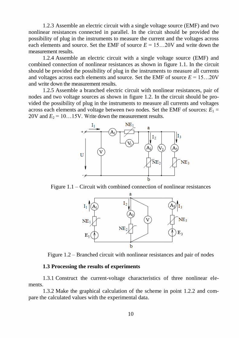
combined connection of nonlinear resistances as shown in figure 1.1. In the circuit

should be provided the possibility of plug in the instruments to measure all currents

and voltages across each elements and source. Set the EMF of source E = 15…20V

and write down the measurement results.

1.2.5 Assemble a branched electric circuit with nonlinear resistances, pair of

nodes and two voltage sources as shown in figure 1.2. In the circuit should be pro-

vided the possibility of plug in the instruments to measure all currents and voltages

across each elements and voltage between two nodes. Set the EMF of sources: E1 =

20V and E2 = 10…15V. Write down the measurement results.

Figure 1.1 – Circuit with combined connection of nonlinear resistances

Figure 1.2 – Branched circuit with nonlinear resistances and pair of nodes

1.3 Processing the results of experiments

1.3.1 Construct the current-voltage characteristics of three nonlinear ele-

ments.

1.3.2 Make the graphical calculation of the scheme in point 1.2.2 and com-

pare the calculated values with the experimental data.

11







1.3.6 Make the conclusions by the work done.

2 Laboratory work №2. Research of electric circuits with valves

The objective of the work is to acquire the skills of experimental research of

electric circuits with valves.


Repeat sections “Analysis of electric circuits at non-sinusoidal EMF and cur-

rents” and “Analysis of electric circuits with valves” of discipline.


1) Which nonlinear element is called an electric valve? Draw its current-

voltage characteristic. Give a definition of the ideal valve.

2) How to construct a time function curve of instantaneous current values in a

circuit with a series-connected electrical valve and an active resistance when sinus-

oidal voltage is applied to them?

3) Draw a half-wave rectifier circuit with an active load resistance. Plot the

curves of the instantaneous values of current and voltage across load. Write down

the expressions for calculating the RMS (effective) value and the constant compo-

nent value (average value per period) of the current and voltage across the load if

assume an ideal rectification conditions.

4) Draw a full-wave rectifier circuit with an active load resistance. Plot the

curves of the instantaneous values of current and voltage across load, write down

the expressions for calculating the RMS value and the constant component of the

current and voltage across the load if assume an ideal rectification conditions.

5) Write down an expression for calculating the effective (RMS) value of the

voltage by using known values of harmonic components.

6) Calculate the values of the apparent S and active P power for the ideal

half-wave and full-wave (bridge scheme) rectifiers with a resistive load. Compare

the values obtained for the two rectifier circuits and evaluate their efficiency.

7) Sketch a circuit for measuring of data to plot the current-voltage character-

istic of a semiconductor diode (valve), connected in series with the resistor, when

the circuit is fed by the smoothly adjustable DC voltage source. Provide in the cir-

cuit diagram necessary measuring instruments.

12


2.2.1 Get the readings for plotting the static current-voltage characteristic of a

semiconductor diode, connected in series with the resistor. The data should be got

for the direct and the reverse connection of the diode when powered from a smooth-

ly adjustable DC voltage source.

2.2.2 Assemble the half-wave rectifier in accordance with the circuit diagram

in figure 2.1. The effective value of the voltage of sinusoidal voltage source should

be set within 10...20 V. Measure the DC component and the effective value of the

AC component of the current and voltage across the load.

2.2.3 Using an oscilloscope, you should get and draw or take pictures from

the screen of the curves of the instantaneous values of the voltage at the input and

the voltage at the output of the rectifier (on the load resistor).

2.2.4 Assemble the full-wave rectifier according to the bridge circuit diagram

shown in figure 2.2. Set the voltage at the input of the rectifier and the load re-

sistance are the same as in point 2.2.2. Measure the DC component and the effective

value of the AC component of the current and voltage across the load.

2.2.5 Using an oscilloscope, you should get and copy or take pictures from

the screen of oscilloscope the curves of the instantaneous values of the voltage at

the input and the voltage at the output of the rectifier.

Figure 2.1 – Circuit diagram of the half-wave rectifier

13

Figure 2.2 – Bridge circuit diagram of the full-wave rectifier


2.3.1 Carry out a graphical calculation for the half-wave rectifier circuit (fig-

ure 2.1), using the current-voltage characteristic constructed by readings of the point

2.2.1. Compare the shape of the acquired current curve with the oscillogram of the

voltage across the load resistor obtained in point 2.2.3.

2.3.2 Calculate the RMS value of the voltage across the load U2 using the

value of U20 DC component measured in point 2.2.2 and the RMS value of U2~ AC

component and compare it with the RMS value of the source voltage.

2.3.3 Calculate the apparent power of the power source S and the active pow-

er of the load P using the readings measured in point 2.2.2 and compare them with

the corresponding values calculated for an ideal half-wave rectifier by the expres-

sions given in 6 section of the preparation for the work.

2.3.4 Calculate the RMS value of the voltage across the load U2 using the

value of U20 DC component measured in point 2.2.4 and the RMS value of U2~ AC

component and compare it with the RMS value of the source voltage.

2.3.5 Calculate the apparent power of the power source S and the active pow-

er of the load P using the readings measured in point 2.2.4 and compare them with

the corresponding values calculated for an ideal full-wave rectifier by the expres-

sions given in 6 section of the preparation for the work.

2.3.6 Compare the results obtained for half- and full-wave rectifiers, and

evaluate their efficiency factors.

2.3.7 Make the conclusions by the work done.

14

3 Laboratory work №3. Research of the voltage ferroresonance phenom-

enon

The objective of the work is to acquire the skills of experimental research of

nonlinear electric circuits at the ferroresonant mode.


Repeat section “Analysis of the ferroresonance phenomenon” of discipline.


1) Which components should include an electrical circuit in order to make it

possible for the phenomenon of voltage ferroresonance?

2) Why is the phenomenon of a current jump in a ferroresonant circuit also

called the phenomenon of phase overturning? Construct phasor diagrams of equiva-

lent sinusoidal voltages of the fundamental harmonic for two modes: before the cur-

rent jump and after.

3) How to choose the value of the capacitor capacitance to ferroresonance

phenomenon occurred and was an abrupt change in current in the circuit?

4) Construct a current-voltage characteristic of a serial ferroresonant circuit.

Analyze the change in current at a smooth increasing in the value of the input volt-

age and then at smooth reducing of it.

5) Draw a scheme to getting data for constructing the current-voltage charac-

teristic of an inductor with a ferromagnetic core, providing it with the necessary

measuring instruments.

6) Draw the following schemes:

a) to getting data for constructing the current-voltage characteristic of a se-

ries-connected inductor with a ferromagnetic core and a capacitor (figure 3.1);

b) to getting data for plotting the curve of the dependence of the total voltage

versus the current in the circuit at a smooth change in the current (figure 3.2);

c) of the ferroresonant voltage regulator (figure 3.3).

Figure 3.1 – Scheme of the ferroresonant circuit with voltage power source

15

Figure 3.2 – Scheme of the ferroresonant circuit with current power source

Figure 3.3 – Scheme of the ferroresonant voltage regulator

Table 3.1 – Experimental data of the scheme in figure 3.1

U, V I, mA UL, V UC, V


I, mA

U, V


U1, V

U2, V


3.2.1 Assemble the circuit in accordance with the scheme of point 5 of the

preparation for work. Take the readings of the instruments and plot the current-

voltage characteristic of the inductor with a ferromagnetic core (5 ... 7 measure-

ments). Plugin a capacitor in the circuit instead of the inductor, take the readings of

the instruments and plot the current-voltage characteristic of the capacitor (two

measurements are sufficient, since the capacitor characteristic is a straight line). Plot

16

the current-voltage characteristic of the capacitor in the same figure that the current-

voltage characteristic of the inductor.

Note. The current-voltage characteristic of the capacitor must cross the cur-

rent-voltage characteristic of the inductor.

3.2.2 Assemble the circuit according to the scheme of section 6a of prepara-

tion for work (figure 3.1).

3.2.3 Gradually increasing the total voltage from zero to 30...40 V, and then

gradually decreasing it, take the current and voltage readings of the coil and capaci-

tor versus the supply voltage. It is necessary to make at least 7...8 measurements be-

fore and after the current jump with an increase in the total voltage, and also at least

7...8 measurements with a decrease in the total voltage.

Note. When there is a sharp current jump with a smooth increase in the sup-

ply voltage, the total voltage is reduced due to an increase in the voltage drop in the

generator.

Before writing the readings of the measuring instruments after the current

jump, it is necessary to restore the value of the supply voltage, which was immedi-

ately before the current jump. Similarly, we should proceed with the reverse current

jump, which occurs when the voltage decreases.

Write down the measurement results in table 3.1.

3.2.4 Assemble the circuit according to the scheme of section 6b of prepara-

tion for work (figure 3.2).

3.2.5 Take the readings for plotting the curve of the dependence of the total

voltage (across the coil and the capacitor) versus the current with a smoothly change

in the current through the circuit. Write down the results of measurements in table

3.2.

Note. For smooth regulation of the current, additional resistance is connected

in series with the generator, so that together with the resistance the generator can be

considered as an artificial source of current. The value of the resistance is chosen as

low as possible, but such that there are no current jumps with a smooth change in

the supply voltage of the circuit. A voltmeter measuring the total voltage of the cir-

cuit must not take into account the voltage drop across the resistance.

3.2.6 Assemble the ferroresonant voltage regulator according to the scheme

of section 6c of preparation for work (figure 3.3). Plug in parallel to the coil of in-

ductance with a ferromagnetic core the resistors bank as a load of regulator.

3.2.7 Take the readings of the dependence of the load voltage versus the input

voltage of the circuit. First set the maximum value of the input voltage and then

smoothly reduce it until the voltage jump on the load occur (make the 5 ... 7 meas-

urements). Write down the readings in table 3.3.


3.3.1 Construct on same graph the current-voltage characteristics of the

whole circuit, of the inductor and of the capacitor according to the results obtained

in point 3.2.3.

17

3.3.2 Based on the results obtained in point 3.2.5, plot the curve of the input

voltage versus current.

3.3.3 According to the data of point 3.2.7, plot the curve of dependence the

load voltage versus of the supply voltage. Explain the dependence obtained. Calcu-

late the stabilization coefficient.

3.3.4 Make conclusions on the work done: compare the idealized current-

voltage characteristic of the circuit with the experimentally obtained, when the volt-

age at the input of the circuit smoothly changes, explain the difference between

them (point 3.3.1). Compare the experimental curve obtained in point 3.3.1 with the

curve of the dependence of the input voltage versus the current, obtained in point

3.3.2, explain their difference.

3.4 Methodological guidelines

The stabilization coefficient is calculated by the formula:

1 2.

1 2

stab

U Uk

U U

,

where U1 – the input voltage of the circuit;

U2 – the output voltage (voltage across the load);

ΔU1 and ΔU2 – changes in the voltage across input and output of the circuit

(figure 3.4).

Figure 3.4 – Dependence of output voltage versus input voltage of regulator

4 Laboratory work №4. Research of the plane-parallel electrostatic field

of a two-wire line

The objective of the work is to obtain the skills of experimental research of a

plane-parallel electrostatic field of a two-wire line using computer simulation.


Repeat the following sections of the discipline: the field of an infinitely long

uniformly charged axis, the field of parallel oppositely charged axes and the field of

the two-wire line [R.3, 4]. Familiarize with the description of the “The field theory”

18

computer application’s interface and with the methodical guidelines for the carrying

out calculations and experiments.

Carry out the following assignments in written form:

1) Write down the formulas for calculating the electrostatic field strength

and potential of the infinitely long uniformly charged axis.

2) Write the formulas for calculating the electrostatic field strength and po-

tential of the two parallel infinitely long oppositely charged axes.

3) Write the boundary conditions for any point on the surface of conductors.

4) In accordance with the initial data of the assignment option (table 4.1),

calculate distances a, S1 and S2. Write down the calculation results in table 4.2.

5) Write down the formula for calculating the capacitance of a two-wire line.

In accordance with the initial data of the assignment option (table 4.1), calculate the

capacitance of the two-wire line. Write down the calculation results in table 4.2.

6) Write formulas for calculating the potentials of points on the surface of

wires φ1 and φ2. In accordance with the initial data of the assignment option (table

4.1), calculate the potentials of any points on the surface of wires φ1 and φ2. Write

down the calculation results in table 4.2.

7) Write down the formulas for calculating the electrostatic field strengths

on the conductor surface at following points: M, N, L and K. Calculate, according to

the initial data of the assignment option (table 4.1), the electrostatic field strengths at

these points. Write down the results of calculations in table 4.2.

8) Write down the formulas for calculating the density of free electric charge

on the conductor’s surface. In accordance with the initial data of the assignment op-

tion (table 4.1), calculate the free electric charge densities on the conductor’s sur-

face at points M, N, L, and K. Write down the calculation results in table 4.2.

9) Give the definition of a plane-parallel field.

10) Give the definition of the equipotential and strength lines of the electro-

static field. Qualitatively plot a pattern of the electrostatic field of a two-wire line.

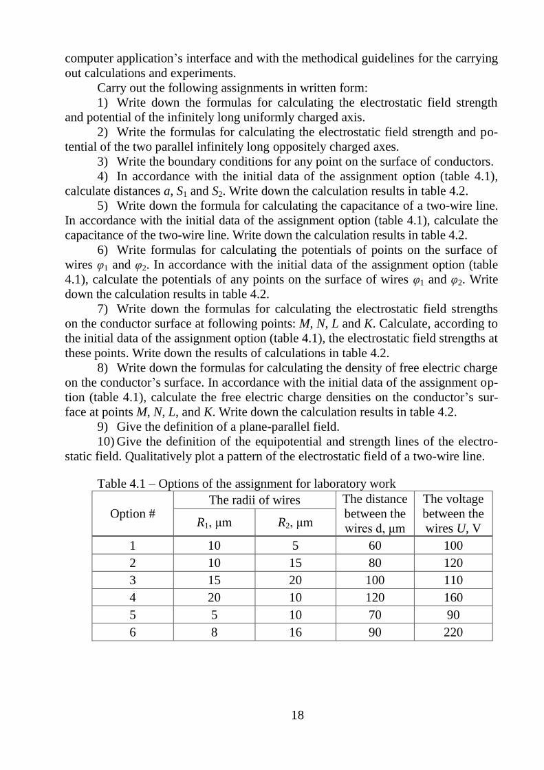
Table 4.1 – Options of the assignment for laboratory work

Option # The radii of wires The distance

between the

wires d, μm

The voltage

between the

wires U, V R1, μm R2, μm

1 10 5 60 100

2 10 15 80 120

3 15 20 100 110

4 20 10 120 160

5 5 10 70 90

6 8 16 90 220

19


4.2.1 Launch the “Field Theory” application by clicking left mouse button on

the computer desktop shortcut (figure 4.1). The main program window opens (fig-

ure 4.2).

Figure 4.1 – The desktop shortcut of the “Field theory” application

4.2.2 Set the data of the wire radii R1, R2 and the distance d according to the

assignment option.

4.2.3 Construct a two-wire line in the workspace by clicking the “Build” but-

ton with the left mouse button. A two-wire line appears on the screen (figure 4.3).

4.2.4 Determine the geometric parameters of the line: a – the distance be-

tween the electrical axis and the plane of the zero potential, S1, S2 – distances be-

tween the geometric axes of wires and the plane of the zero potential. Write down

the resulting values of a, S1 and S2 in table 4.2.

4.2.5 Set the voltage between the wires, according to the assignment option,

using a voltage source (figure 4.2, description of the application interface and meth-

odological guidelines).

4.2.6 Get the image of the electric axes by clicking the left mouse button on

the “Axis” button.

4.2.7 Measure the capacitance of the two-wire line per unit length. The result-

ing capacitance value write down in table 4.2.

4.2.8 Measure the electrostatic field strength on the wire surface at given

points: M, N, L and K. Write down the results of measurements in table 4.2.

4.2.9 Plot the pattern of equipotential lines of the electrostatic field of two-

wire line with a step Δφ = 10…20 V as instructed by the teacher.

4.2.10 Plot a pattern of the strength lines of the electrostatic field of a two-

wire line.

4.2.11 Save the resulting pattern of the electrostatic field of the two-wire line

by clicking the left button of the mouse on the button “Export to *.bmp”.


4.3.1 Perform a theoretical calculation of the geometric distances of the two-

wire computational scheme: a, S1 and S2. Write down the calculation results in table

20

4.2 in the column “Theoretical calculation”. Determine the same distances: a, S1 and

S2 in the “Field theory” application on the computer, write down the obtain results

in table 4.2 in the “Experiment” column. Compare the results.

4.3.2 Perform a theoretical calculation of the capacitance of a two-wire line

and potentials on the surface of wires φ1, φ2, write down the calculation results in

table 4.2, in the column “Theoretical calculation”. Measure the capacitance of the

two-wire line and the potentials of points on the wires surface φ1, φ2 in a computer

application and write down the results in table 4.2 in the column “Experiment”.

Compare the results.

4.3.3 Perform a theoretical calculation of the electrostatic field strengths on

the surface of the wires at given points: M, N, L and K. Write down the calculation

results in table 4.2, in the column “Theoretical calculation”. Measure the electrostat-

ic field strengths on the surface of the wires at given points: M, N, L and K. Write

down the obtain results in table 4.2, in the “Experiment” column. Compare the re-

sults.

4.3.4 Perform a theoretical calculation of the density of free electric charge

on the wire’s surface at given points: M, N, L and K. Write down the calculation re-

sults in table 4.2, in the column “Theoretical calculation”. Measure the density of

free electric charge on the wire’s surface at given points: M, N, L and K. Write

down the obtain results in table 4.2, in the “Experiment” column. Compare the re-

sults.

4.3.5 Save and print the experimentally obtained pattern of a plane-parallel

electrostatic field of a two-wire line.

4.3.6 Add the resulting pattern by plotting manually the strength lines of elec-

trostatic field on it.

4.3.7 Make conclusions about the work done.

Table 4.2

Geometric distances of the two-wire

computational scheme: a, S1, S2. Po-

tentials of wires φ1, φ2. Capacitance

C, strength E and density of free

electric charge σ

Theoretical

calculation Experiment

a, m

S1, m

S2, m

φ1, V

φ2, V

C, F/m

EM, V/m

EN, V/m

EL, V/m

EK, V/m

σM, C/m2

21

σN, C/m2

σL, C/m2

σK, C/m2

4.4 Interface description of the “Field theory” computer application

The main window of the application interface (figure 4.2) contains a work-

space and two side panels on which the measuring instruments and control buttons

are located. The workspace has a grid, which appearance can be changed by the

“Grid” button.

At the top of the left sidebar of the main program window are the drawing

tools that contain the following buttons:

− is a button to drawing points in the workspace;

− is a button (eraser) to clean the working area from the wrongly

put points;

− is a button to drawing straight lines connecting neighboring

points in the workspace;

− is a button (eraser) to clean the working area of the wrongly

drawn segments of straight lines;

− is a button to cleaning the working area from the equipotential

lines and lines of force of electric field;

− is a button to drawing the lines of force of electric field;

− is a button to resizing the grid cell of the workspace;

− is a button to displaying the position of electric axes.

The following tools are also located on the left side panel:

− is an instrument to measuring the electric field strength,

it is activated by clicking the left mouse button on the

“V/m” button.

− is an instrument to calculating the geometric dimensions

of a two-wire line’s model;

− is a button to access the area in which the buttons for

zooming are located: “+” and “–”.

22

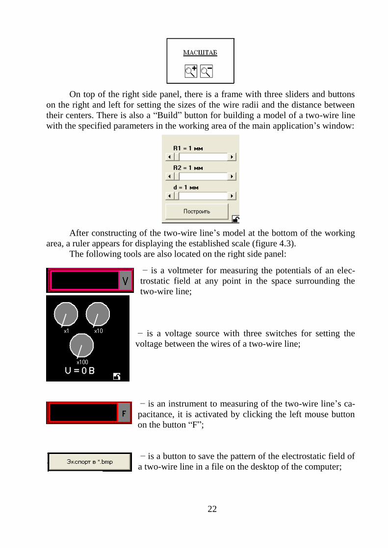
On top of the right side panel, there is a frame with three sliders and buttons

on the right and left for setting the sizes of the wire radii and the distance between

their centers. There is also a “Build” button for building a model of a two-wire line

with the specified parameters in the working area of the main application’s window:

After constructing of the two-wire line’s model at the bottom of the working

area, a ruler appears for displaying the established scale (figure 4.3).

The following tools are also located on the right side panel:

− is a voltmeter for measuring the potentials of an elec-

trostatic field at any point in the space surrounding the

two-wire line;

− is a voltage source with three switches for setting the

voltage between the wires of a two-wire line;

− is an instrument to measuring of the two-wire line’s ca-

pacitance, it is activated by clicking the left mouse button

on the button “F”;

− is a button to save the pattern of the electrostatic field of

a two-wire line in a file on the desktop of the computer;

23

− is a lock button for locking and unlocking of the preset

parameters of two-wire line and source voltage.

Figure 4.2 – The main window of the “Field theory” application

Figure 4.3 – Two-wire line’s model

24

4.5 Methodological guidelines

Read the description of the program “Field theory”.

To set the radius of the wires R1, R2 and the distance between wires d, the

sliders and the buttons on the right and left are used, which are increased or de-

creased the values of R1, R2 and d, accordingly. To prevent accidental changes of

the two-wire line’s settings, you need to click the left mouse button on the “lock”

button. To build a two-wire line’s model, click the “Build” button (figure 4.3).

To calculate the geometric dimensions of the line’s model, click on the “Ge-

ometry” button, as a result, a region with the dimensions a, S1 and S2 will be

opened.

Value of the voltage between the wires is set by means of three voltage

source switches. To increase the voltage, click the left mouse button, and to de-

crease the voltage, right-click on the arrow of the corresponding source switch.

The image of the electric axes of the line’s model can be obtained by clicking

the left mouse button on the “Axis” button (figure 4.3), you can also remove the

electric axes by clicking the “Axis” button again with the left mouse button.

The capacitance of a two-wire line per length unit can be measured using of

an appropriate instrument, by clicking on the “F” button with the left mouse button

(figure 4.3).

You can measure the strength of the electrostatic field at any point in the

space surrounding the two-wire line by activating the corresponding instrument by

clicking left mouse button on the “V/m” button. Then place the cursor in the point

of space where you want to measure the electrostatic field strength and click on the

right mouse button. The value of the strength appears on the instrument panel (fig-

ure 4.3).

To determine position of the points of the equipotential line of the two-wire

line’s electrostatic field, a voltmeter is used, with the help of which the potentials of

the points surrounding the line of space can be measured. To draw an equipotential

line’s point, click the left mouse on the button for drawing the points, which is lo-

cated at the top of the left panel: the “drawing tools” (see the program description).

Then find the point with the given potential, moving the cursor and watching the

voltmeter’s readings. When the voltmeter’s readings are matched with given poten-

tial’s value click the left mouse button to place the found point in the space. Errone-

ously drawn points can be deleted using the (eraser) button located in the same

place.

Obtained points of future equipotential can be connected with each other by

straight-line segments. To do this, use the left mouse button to activate the tool for

drawing line segments, then left-click on two adjacent points with the same poten-

tials, and they are connected by a straight-line segment. The erroneously drawn

segments can be deleted using the (eraser) button.

To build the lines of force of electrostatic field click the “E” button with the

left mouse button. Specify the required number of lines of force in an appeared dia-

25

log box (figure 4.4) and click “OK” button. To remove the lines of force, you can

re-click the “E” button with the left mouse button.

Figure 4.4

The obtained pattern of the electrostatic field of the two-wire line can be

saved by clicking the left mouse button on the “Export to *.bmp” button. To print a

saved field’s pattern it is most convenient to open it with the Paint application.

The lines of force of electrostatic field of a two-wire line can be constructed

manually on the printed sheet with pattern, which was only equipotential lines are

constructed. One of the lines of force is a straight line connecting electrical axes.

All other lines of force are arcs of a circle passing through electric axes, with cen-

ters lying on the line of zero potential, and are defined by equation 2 2 2 2

0 0( )x y y a y , where 0y is the center of an arc of a circle. The lines of

force are perpendicular to the equipotential lines and are drawn so that between

each pair of adjacent lines there is an equal part of the total flux of the field strength

vector.

It is possible completely to clean the screen from equipotential lines and lines

of force by clicking the left mouse on the button “Cls”.

4.6 Methodological guidelines for the theoretical calculation

The geometric dimensions of the two-wire line’s model a, S1, и S2 (figure

4.5) are calculated by formulas: 2 2 2 2 2 2

2 2 2 21 2 2 11 2 1 1 2 2, ,

2 2

d R R d R RS S a S R S R

d d

,

where d = S1 + S2 is the distance between the geometric axes of the wires;

S1, S2 are the distances from the geometric axes of the wires to the plane of

zero potential;

R1, R2 are the radii of wires;

а is a distance of electric axes from plane of zero potential.

The capacitance of a two-wire line C is determined by expression:

26

0

1 2

1 2

2

( ) ( )ln

CS a S a

R R

,

where

ε0 = 8,854∙10–12

F/m is a permittivity of vacuum;

ε = 1 is a relative permittivity of air.

The potentials of points on the surface of wires φ1, φ2 are calculated by for-

mulas:

11

0 1

ln2

C U S a

R

,

22

0 2

ln2

C U R

S a

.

The electric field strength at the wire’s surface at the points M, N, L and K are

calculated by the formulas (figure 4.5):

0

1 1

2 2M

M M

C UE

R R a

;

0

1 1

2 2N

N N

C UE

R a R

;

0

1 1

2 2L

L L

C UE

R R a

;

0

1 1

2 2K

K K

C UE

R a R

;

where

1 1MR S a R is a distance from the positive electric axis to the point M;

1 1( )NR R S a is a distance from the positive electric axis to the point

N;

2 2( )LR R S a is a distance from the positive electric axis to the point

L;

2 2KR S a R is a distance from the positive electric axis to the point K.

The electric charge density at the wire surface at points M, N, L and K are

calculated by formulas:

0M ME ; 0N NE ; 0L LE ; 0K KE .

27

Figure 4.5 – The calculation scheme of the two-wire line’s model

References

Main references

1 John Bird. Electrical Circuit Theory and Technology. – Fifth edition, 2 Park

Square, Milton Park, Abingdon, Oxon OX14 4RN, UK: 2014. – 769 p.

28

2 Fundamentals of Electric Circuits / Charles K. Alexander, Matthew N. O.

Sadiku. – Fifth edition 2013. – 995 p.

3 Electromagnetic Field Theory. Bo Thide and Mattias Waldenvik. – Uppsa-

la, Sweden, 2012. – 298 p.

4 Richard Fitzpatrick. Maxwell’s Equations and the Principles of Electro-

magnetism. – Infinity Science Press LLC: Hingham, 2008. – 438 p.

Additional references

5 Бессонов Л. А. ТОЭ. Электрические цепи: Учебник. – 11-е изд., пере-

раб. и доп. – М.: Гардарики, 2007. – 701 с.: ил.

6 Бессонов Л. А. ТОЭ. Электромагнитное поле: Учебник. – 10-е изд.,

стереотипное. – М.: Гардарики, 2003. – 317 с.: ил.

7 Теоретические основы электротехники: в 3-х т. Учебник для вузов.

Том 2. – 4-е изд. / К. С. Демирчян, Л. Р. Нейман, Н. В. Коровкин, В. Л. Чечу-

рин. – СПб.: Питер, 2003. – 576 с.: ил.

8 Теоретические основы электротехники: в 3-х т. Учебник для вузов.

Том 3. – 4-е изд. / К. С. Демирчян, Л. Р. Нейман, Н. В. Коровкин, В. Л. Чечу-

рин. – СПб.: Питер, 2003. – 377 с.: ил.

9 Денисенко В. И., Зуслина Е. Х. ТОЭ. Учебное пособие. – Алматы:

АИЭС, 2000. – 83 с.

non-commercial joint stock company almaty university of

Documents