non-linear regression models - krikamol.orgkrikamol.org/courses/2016/scma292/lecture07.pdfnon-linear...
TRANSCRIPT

Non-linear Regression ModelsSCMA292 Mathematical Modeling : Machine Learning
Krikamol MuandetDepartment of Mathematics
Faculty of Science, Mahidol University
February 25, 2016

Outline
A Quick Recap
Nonlinear Feature Representation
Basis Functions
Linear Regression with Basis Functions
Model Selection

A Quick Recap
▶ Basics of mathematical modelling and machine learning▶ Probability theory, ML and MAP estimates▶ Regression problem
▶ Least square regression▶ Ridge regression▶ Overfitting and regularization
▶ Classification problem▶ Naïve Bayes : text classification▶ Logistic regression▶ Perceptron and multi-layer perceptron

Outline
A Quick Recap
Nonlinear Feature Representation
Basis Functions
Linear Regression with Basis Functions
Model Selection

Complexity is just a matter of perspective.

MLP as Feature Map
h2
h1
hK
x1
x2
xd
y...
new input
Perceptron
y = f(h(x)) = f(
K∑i=1
wk1hk(x)), hk(x) = h
(w0k +
d∑i=1
wikxi
)

MLP as Feature Map
h2
h1
hK
x1
x2
xd
y...
new input
Perceptron
y = f(h(x)) = f(
K∑i=1
wk1hk(x)), hk(x) = h
(w0k +
d∑i=1
wikxi
)

MLP as Feature Map
h2
h1
hK
x1
x2
xd
y...
new input
Perceptron
y = f(h(x)) = f(
K∑i=1
wk1hk(x)), hk(x) = h
(w0k +
d∑i=1
wikxi
)

MLP as Feature Map
h2
h1
hK
x1
x2
xd
y...
new input
Perceptron
y = f(h(x)) = f(
K∑i=1
wk1hk(x)), hk(x) = h
(w0k +
d∑i=1
wikxi
)

MLP as Feature Map
h2
h1
hK
x1
x2
xd
y...
new input
Perceptron
y = f(h(x)) = f(
K∑i=1
wk1hk(x)), hk(x) = h
(w0k +
d∑i=1
wikxi
)

MLP as Feature Map
h2
h1
hK
x1
x2
xd
y...
new input
Perceptron
y = f(h(x)) = f(
K∑i=1
wk1hk(x)), hk(x) = h
(w0k +
d∑i=1
wikxi
)

MLP as Feature Map▶ For each data point x, the MLP transforms it into a new
vector Φ(x) given by
x 7→ Φ(x) ≜
h1(x)h2(x)
...hK(x)
=
h(w01 + ∑d
i=1 wi1xi)
h(w02 + ∑di=1 wi2xi)
...h(w0K + ∑d
i=1 wiKxi)
▶ Let the output activation function f be a step function
z
y
y =
1 if w0 + ∑Kk=1 wkhk(x) > 0
0 if w0 + ∑Kk=1 wkhk(x) ≤ 0

Nonlinear Feature Map

Outline
A Quick Recap
Nonlinear Feature Representation
Basis Functions
Linear Regression with Basis Functions
Model Selection

Linear Regression
▶ The simplest model : f(x) = w0 + w1x
▶ It can be extended to polynomial of higer degree
f(x) = w0 + w1x + w2x2 + w3x3 + · · ·wpxp =p∑j=1
wjxj
▶ A linear combination of nonlinear functions of x called basisfunction, i.e., ϕj(x) = xj.
▶ Linear functions of parameters (w0,w1, . . . ,wp), yetnon-linear w.r.t. input variables x.

Linear Regression
▶ The simplest model : f(x) = w0 + w1x▶ It can be extended to polynomial of higer degree
f(x) = w0 + w1x + w2x2 + w3x3 + · · ·wpxp =p∑j=1
wjxj
▶ A linear combination of nonlinear functions of x called basisfunction, i.e., ϕj(x) = xj.
▶ Linear functions of parameters (w0,w1, . . . ,wp), yetnon-linear w.r.t. input variables x.

Linear Regression with Basis FunctionsLet extend x via nonlinear functions ϕj
f(x) =M∑j=1
wjϕj(x) = w⊤Φ(x)
where w = (w1, . . . ,wM) and Φ = (ϕ1(x), . . . , ϕM(x)).▶ The function ϕj are called basis functions▶ In most cases, ϕj are fixed prior of learning, but sometimes
we learn them directly from the data, e.g., deep learning.from the data.
Exercise: find the basis functions ϕj that correspond to the linearregression model.

Polynomial Basis
▶ Polynomial basis of degree M for univariate variable x
ϕj(x) = xj, j = 1, 2, . . . ,M
▶ Polynomial basis of degree M for multivariate variable x
ϕj(x) = ∥x∥j =
(√x2
1 + x22 + · · ·+ x2
d
)j
▶ correponds to fitting the polynomial function of degree M
pM(x) = a0 + a1x + a2x2 + · · ·+ aMxM

Polynomial Basis
x
ϕ(x)
ϕ0
ϕ1ϕ2

Gaussian Radial Basis
▶ Gaussian radial basis for univariate variable x
ϕj(x) = exp(− (x − µj)2
2σ2
)▶ Polynomial basis of degree M for multivariate variable x
ϕj(x) = exp(−1
2(x −µj)⊤Σ−1(x −µj)
)▶ Choice of parameters
▶ µj : the locations of the basis functions▶ σ : the spatial scale of the basis functions

Gaussian Radial Basis
x
ϕ(x)ϕ1 ϕ2 ϕ3 ϕ4

Sigmoidal Basis
▶ Sigmoid basis function for univariate variable x
ϕj(x) = σ
(x − µjσ
)where σ(z) = 1
1 + exp(−z)
x
ϕ(x)

Other Basis Functions
▶ Fourier basis : good representation for oscillatory functions▶ Wavelet basis : good representation for functions localized
at multiple scales, e.g., images and time series.

Least Square with Basis FunctionsGiven M basis functions ϕj, the least square loss function is
L(w) =12
n∑i=1
(yi − fw(xi))2 =
12
n∑i=1
(yi − w⊤Φ(xi))2
Exercises:▶ write the least square solution given the basis function ϕ
▶ write the ridge regression solution given the basis function ϕ
Φ(X) ≜
Φ(x1)
Φ(x2)...
Φ(xn)
=
ϕ1(x1) ϕ2(x1) · · · ϕM(x1)
ϕ1(x2) ϕ2(x2) · · · ϕM(x2)...
ϕ1(xn) ϕ2(xn) · · · ϕM(xn)

Least Square with Basis Functions
The least square objective with basis functions ϕ is
L(w) =12(y − Φ(X)w)⊤(y − Φ(X)w).
The solution w = arg minw L(w) is given by
(Φ(X)⊤Φ(X))w = Φ(X)⊤yw = (Φ(X)⊤Φ(X))−1Φ(X)⊤y.
Ridge regression with basis functions
w = (Φ(X)⊤Φ(X) + λI)−1Φ(X)⊤y

Least Square with Basis Functions▶ We need to compute the inverse of M := Φ(X)⊤Φ(X) for
least square and M := Φ(X)⊤Φ(X) + λI for ridge regression▶ A simple trick
w =(
Φ(X)⊤Φ(X) + λI)−1
Φ(X)y
= Φ(X)(
Φ(X)Φ(X)⊤ + λI)−1
y
=n∑i=1
αiΦ(xi)
where αi := ((Φ(X)Φ(X)⊤ + λI
)−1 y)i.▶ For a test point x∗,
f(x∗) = w⊤Φ(x∗) = ∑ni=1 αiΦ(xi)⊤Φ(x∗).

Classification

Classification
ϕ : (x1, x2) 7−→ (x21, x2
2,√
2x1x2)

Curse of Dimensionality
▶ For polynomial basis function, the number of features growspolynomially with the degree and exponentially with thenumber of input features.
▶ For M = 3 and d = 3
ϕj(x) = (x1, x2, x3, x1x2, x1x3, x2x3, x21, x2
2, x23)
▶ The number of quadratic terms is 1 + d + d(d − 1)/2 + d.

Curse of Dimensionality
source : http://www.iro.umontreal.ca/~bengioy


Sound Pressure of Dolphin Sonar
http://www.statsci.org/data/general/dolphin.html
0 2 4 6 8 10 12 14 16 18
Range
180
190
200
210
220
230
240
SoundPre
ssure
Sound pressure of sonar signals (“clicks”) from a dolphin atvarious ranges to target.
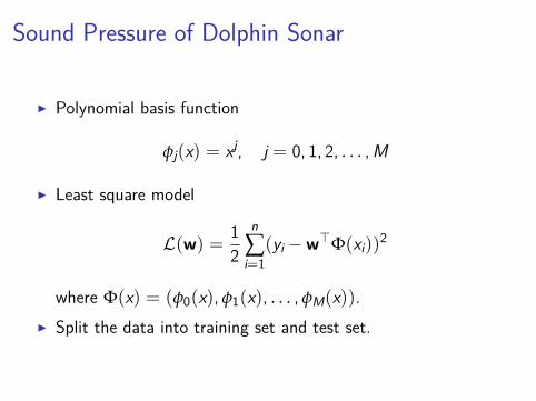
Sound Pressure of Dolphin Sonar
▶ Polynomial basis function
ϕj(x) = xj, j = 0, 1, 2, . . . ,M
▶ Least square model
L(w) =12
n∑i=1
(yi − w⊤Φ(xi))2
where Φ(x) = (ϕ0(x), ϕ1(x), . . . , ϕM(x)).▶ Split the data into training set and test set.

Sound Pressure of Dolphin Sonar
M = 1
0 2 4 6 8 10 12 14 16 18
Range
180
190
200
210
220
230
240
SoundPre
ssure
score on training set : 0.5366

Sound Pressure of Dolphin Sonar
M = 2
0 2 4 6 8 10 12 14 16 18
Range
180
190
200
210
220
230
240
SoundPre
ssure
score on training set : 0.5781

Sound Pressure of Dolphin Sonar
M = 3
0 2 4 6 8 10 12 14 16 18
Range
170
180
190
200
210
220
230
240
250
260
SoundPre
ssure
score on training set : 0.6079

Sound Pressure of Dolphin Sonar
M = 4
0 2 4 6 8 10 12 14 16 18
Range
160
170
180
190
200
210
220
230
240
SoundPre
ssure
score on training set : 0.6164

Sound Pressure of Dolphin Sonar
M = 5
0 2 4 6 8 10 12 14 16 18
Range
160
180
200
220
240
260
280
300
320
340
SoundPre
ssure
score on training set : 0.6194
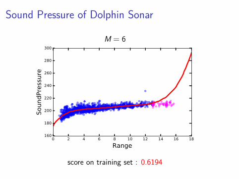
Sound Pressure of Dolphin Sonar
M = 6
0 2 4 6 8 10 12 14 16 18
Range
160
180
200
220
240
260
280
300
SoundPre
ssure
score on training set : 0.6194

Sound Pressure of Dolphin Sonar
M = 7
0 2 4 6 8 10 12 14 16 18
Range
1000
800
600
400
200
0
200
400
SoundPre
ssure
score on training set : 0.6209

Sound Pressure of Dolphin Sonar
0 1 2 3 4 5 6 7 8
degree of polynomial
0.50
0.52
0.54
0.56
0.58
0.60
0.62
0.64
0.66tr
ain
ing s
core
Which degree of polynomial should we pick?

Sound Pressure of Dolphin Sonar
0 1 2 3 4 5 6 7 8
degree of polynomial
0.50
0.52
0.54
0.56
0.58
0.60
0.62
0.64
0.66
score
training score
0 1 2 3 4 5 6 7 8
degree of polynomial
500
400
300
200
100
0
100
score
test score
Which degree of polynomial should we pick?

Outline
A Quick Recap
Nonlinear Feature Representation
Basis Functions
Linear Regression with Basis Functions
Model Selection

Model SelectionMost ML models depends on some unknown parameters, e.g., λ.
How to choose the best parameter values?

Model Selection

K-Fold Cross Validation

K-Fold Cross Validation1. Partition D = {(x1, y1), (x2, y2), . . . , (xn, yn)} into K
separate sets of equal size.▶ D = {D1,D2, . . . ,DK} with |Dk| ≈ n/K
2. For each k = 1, 2, . . . ,K▶ fit the model f(−k)
λ onD(−k) = {D1, . . . ,Dk−1,Dk+1, . . . ,DK}
▶ Compute the cross-validation error
CVλ(k) =1
|Dk| ∑(x,y)∈Dk
(y − f(−k)λ (x))2
3. Compute overall cross-validation error :
CVλ =1K
K∑i=1
CVλ(k)
4. Pick λ∗ with the smallest cross-validation error.

Model Selection
0 2 4 6 8 10 12 14 16 18
Range
180
190
200
210
220
230
240
SoundPre
ssure
training set
test set
validation set
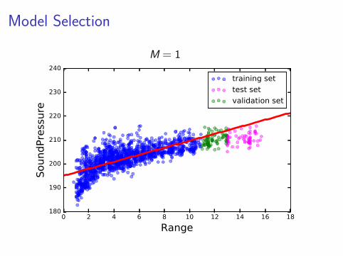
Model Selection
M = 1
0 2 4 6 8 10 12 14 16 18
Range
180
190
200
210
220
230
240
SoundPre
ssure
training set
test set
validation set

Model Selection
M = 2
0 2 4 6 8 10 12 14 16 18
Range
180
190
200
210
220
230
240
SoundPre
ssure
training set
test set
validation set

Model Selection
M = 3
0 2 4 6 8 10 12 14 16 18
Range
160
180
200
220
240
260
280
300
SoundPre
ssure
training set
test set
validation set

Model Selection
M = 4
0 2 4 6 8 10 12 14 16 18
Range
0
50
100
150
200
250
SoundPre
ssure
training set
test set
validation set

Model Selection
M = 5
0 2 4 6 8 10 12 14 16 18
Range
170
180
190
200
210
220
230
240
SoundPre
ssure
training set
test set
validation set

Model Selection
M = 6
0 2 4 6 8 10 12 14 16 18
Range
0
200
400
600
800
1000
1200
1400
SoundPre
ssure
training set
test set
validation set

Model Selection
M = 7
0 2 4 6 8 10 12 14 16 18
Range
4000
3500
3000
2500
2000
1500
1000
500
0
500
SoundPre
ssure
training set
test set
validation set

Model Selection
0 1 2 3 4 5 6 7 8
degree of polynomial
0.46
0.48
0.50
0.52
0.54
0.56
0.58
0.60
0.62
score
training score
0 1 2 3 4 5 6 7 8
degree of polynomial
30
25
20
15
10
5
0
5
score
validation score
Which degree of polynomial should we pick?

Model Selection
0 1 2 3 4 5 6 7 8
degree of polynomial
20000
15000
10000
5000
0
5000
score
training score
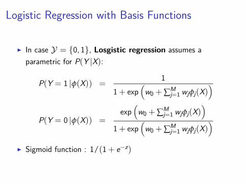
Logistic Regression with Basis Functions
▶ In case Y = {0, 1}, Losgistic regression assumes aparametric for P(Y |X):
P(Y = 1 |ϕ(X)) =1
1 + exp(
w0 + ∑Mj=1 wjϕj(X)
)P(Y = 0 |ϕ(X)) =
exp(
w0 + ∑Mj=1 wjϕj(X)
)1 + exp
(w0 + ∑M
j=1 wjϕj(X))
▶ Sigmoid function : 1/(1 + e−z)

Further Reading
▶ Bishop Ch. 3, sections 3.1 – 3.4 (optional 3.5)

HomeworkAssume the following model
y = fw(x) + ε
where f(x) = w⊤Φ(x) and ε ∼ N (0, σ).1. Find the maximum likelihood (ML) and maximum a
posteriori (MAP) estimates of w when w ∼ N (0, σ)
2. Compare the solutions to the least square solution and ridgeregression
3. Do the same for multiple output setting y = (y1, y2, . . . , ym)
assuming the following model
yi = fwi(x) + ε i, ε i ∼ N (0, σi)