non-stationary flood frequency analysis using additive...

International Journal of Current Engineering and Technology E-ISSN 2277 – 4106, P-ISSN 2347 – 5161 ©2017 INPRESSCO®, All Rights Reserved Available at http://inpressco.com/category/ijcet

Research Article

556| International Journal of Current Engineering and Technology, Vol.7, No.2 (April 2017)

Non-stationary Flood Frequency Analysis using Additive terms for Location, Scale and Shape parameters in the Ouémé River basin (Benin, West Africa) Arcadius Dègan†*, Eric AdéchinaAlamou‡, Yèkambèssoun N’Tcha M’Po‡ and Abel Afoudaϯ

†Laboratory of Applied Energetics and Mechanics, University of Abomey-Calavi, Abomey-Calavi, 01 BP 4521 Cotonou, Benin

‡Laboratory of Applied Hydrology, University of Abomey-Calavi, 01 BP 4521 Cotonou, Benin ϯWest African Science Service Center on Climate Change and Adapted Land Use, University of Abomey-Calavi , 01 BP 4521 Cotonou, Benin

Accepted 10 April 2017, Available online 17 April 2017, Vol.7, No.2 (April 2017)

Abstract Nowadays, the world is changing under climate variability effects and human activities intensification. Continuing to realize flood frequency analysis by considering the stationarity assumption of hydrological time series data, which has been widely used in the past, cannot be further advocated. Hence, it is important to take into account the non-stationary approach in flood frequency analysis. The main focus of this work is to analyse non-stationary flood frequency in the Ouémé River basin. To this end, six hydrometric gauge stations, which have long flood time series data, are considered. Three models are compared at each station to find the more accurate. The three models are the stationary model with low value of AIC according to the distributions of extremes, the non-stationary which use only time for covariate and the non-stationary which use principal components obtained from EOF analysis on the explanatory variables. The explanatory variables are the variables that could explain the evolution of the peak discharge data used. This study considered climate indices like Sea Surface Temperature (SST) and Sea Level Pressure (SLP) indices and daily temperature series. General Additive Models for Location Scale and Shape (GAMLSS) tool help us to perform this non-stationarity in the models. And it is noticed at the end that non-stationary model better fits the data and non-stationary which could represent the subsequent changes is better than the one with time for covariate. Their prediction power has also been tested and it can be retained that for future prediction the non-stationary model with time is better because it is the only one which can perform the analysis. But for past records prediction the non-stationary model which uses principal components as covariates, reproduces well the quantiles. Finally, the differences between the non-stationary quantiles and their equivalents stationary may be important over long periods of time. Keywords: Non-stationary, climates indices, time, GAMLSS, Ouémé basin, peak discharge data. 1. Introduction

1 In the dry tropical West African regions, the development of water resources for agriculture and livestock through small irrigation arrangements requires a good knowledge of hydrological laws and especially exceptional floods features to prevent the risk of destruction of water management and harvesting. Moreover, a good knowledge of hydrological regimes helps to better estimate the annual volumetric contributions, to correctly size the storage structures and to determine their potential, to contribute to the development and to the satisfaction of people's needs (Alamou E., 2011). The frequency analysis (FA) of extreme values (EV) of environmental quantities has been widely used for problems related *Corresponding author: ArcadiusDègan

to engineering design and risk management for buildings, bridges, and urban circulation systems.

The processes and hydrological extremes study at local and regional levels, is performed through the measurement and analysis of different hydro-climatic variables (rainfall, temperature, discharge, etc.). This requires appropriate statistical tools that take into account the interaction between the different variables. Flood frequency analysis (FFA) is most commonly used by engineers and hydrologists worldwide and basically consists of estimating flood peak quantiles for a set of non-exceedance probabilities. Traditional approaches of frequency analysis assume stationary series of observations, and the independence and homogeneity. In other words, the observations should be independent and identically distributed (i.i.d.) (Stedinger and Jery R, 1993, Khaliq et al., 2006). In fact, all water-related

Arcadius Dègan et al Non-stationary Flood Frequency Analysis using Additive terms for Location..


infrastructures were and are currently designed assuming a stationary of hydrological time series. In Hydrology, flood occurrence distribution may change over time (existence of non-stationary) as a result of human activities or because of climate change (Zhang et al., 2001, El Adlouni et al., 2007). In addition, the report of the Intergovernmental Panel for Climate Change–(IPCC) ([IPCC], 2001) concluded to an increase in global temperature with effects on the frequency of extreme events; as well as the potential influence of human activity on climate change or indirectly changing the hydrologic cycle (Zveryaev, 2000), have made the assumption of stationarity widely questionable. Having this in mind, several researchers have begun exploring the validity of this assumption in flood regimes in many regions around the world by considering the effect of natural climate variability (Douglas et al., 2000, Franks and Stewart, 2002, Mudelsee et al., 2003, Milly et al., 2005, Villarini et al., 2009a, Wilson et al., 2010) or land use changes(Hejazi and Markus, 2009, Villarini et al., 2009b, Vogel et al., 2011). These studies have revealed clear violations of the assumption of stationarity, which is consistent with studies that indicate acceleration in the hydrologic cycle (Allen and Smith, 1996, Held and Soden, 2006). It is therefore necessary to develop frequency analysis approaches that take into account the non-stationary series of hydro-climatic data. Such kind of models allow including the effect of different covariates on the variability and evolution of the observed series. Recently, Milly(Milly et al., 2007) stated that the stationary assumption is no longer applicable for water resources risk assessment and planning. This paper develops an innovative approach to provide estimates of hydrologic indicators that would be both reliable and useful for water management in order to adapt to the uncertainties in a changing environment. In the literature, various methodologies based on probabilistic modeling of flood frequency in a non-stationary context have been proposed. For frequency analysis of non-stationary observations, Khaliq(Khaliq et al., 2006) presented a review of various methodologies, including the incorporation of trends in the parameters of the distributions, time-varying moment method, the local likelihood method, and the quantile regression method. Seidou(Seidou et al., 2012) used the non-stationary GEV model to describe the flood peaks which showed that exceedance probabilities on the Kemptville Creek will rise up to 34 % above current levels in 2100 for the return period of 20 years. A lot of studies of FFA under non-stationary conditions have mostly assumed trends in time (Olsen et al., 1998, McNeil and Saladin, 2000, Stedinger and Crainiceanu, 2000, Strupczewski et al., 2001, Renard et al., 2006, He et al., 2006, Leclerc and Ouarda, 2007, Delgado et al., 2010). The time-varying models provide useful tools for reconstructing the behaviour of flood frequency. However, the adoption of predictions from a model that is only time dependent is not entirely correct; trends can change in the short- and long-term

because of climate variability and the intensification of human activities, which are the true drivers. The climate change effect on hydrological variables related to extreme events (annual maximum rainfall, annual extreme discharge, etc.) can be done by studying the existence of trends in the observed series, or by analyzing the studied variables dependence with other climate variables or indices, called covariates (Katz, 1999). For this reason, in the last decade some researchers have explored the possibility of incorporating climate indices as external forcings into models for FFA, assuming linear and nonlinear dependences (El Adlouni et al., 2007, Katz et al., 2002, Sankarasubramanian and Lall, 2003, Kwon et al., 2008, Aissaoui-Fqayeh et al., 2009, Ouarda and El‐Adlouni, 2011). The results showed the feasibility of incorporating climate indices as covariates in the models, and so enabling the models to better describe changes in flood regimes over time by incorporating predictive variables. Furthermore, Yee and Stephenson (Yee and Stephenson, 2007) introduced the classes of vector generalized linear and additive models which allow all parameters of extreme value distributions to be modelled as linear or smooth functions of covariates. Recently, a new class of univariate regression models called the Generalized Additive Model for Location, Scale and Shape parameters (GAMLSS) has been proposed by Rigby and Stasinopoulos (Rigby and Stasinopoulos, 2005) for non-stationary modeling. Compared to classical Generalized Additive Models (Hastie and Tibshirani, 1990), GAMLSS provides a flexible modeling framework. In GAMLSS, the variables of interest can follow a more general distribution other than the exponential family (e.g., Gaussian and exponential), such as highly skewed distributions or kurtosis, which may be more appropriate for modeling the records of interest. In addition, the GAMLSS allows all the parameters of the conditional distribution to be modeled as parametric and/or additive nonparametric (smooth) functions of explanatory variables of interest (Rigby and Stasinopoulos, 2005). Gabriele Villarini(Villarini et al., 2010) used GAMLSS to model seasonal rainfall and temperature over Rome. This author showed that the GAMLSS models represent the magnitude and spread in the seasonal time series with parameters being a smooth function of time or teleconnection indices. GAMLSS model has also been used for flood frequency analysis (Villarini et al., 2009b, López and Francés, 2013). Zhang et al. (Zhang et al., 2015) also used the GAMLSS to model the annual maximum daily precipitation during the time-period 1960 – 2013 in Beijing-Tianjin-Hebei region that has witnessed extensive urban and suburban development over the past 50 years. For implementing non-stationary in modeling the maxima series and find the corresponding return levels, instead of assuming just a linear dependence on time of the parameters of the selected distribution, an optimized cubic spline will



be used to describe the temporal variability of the distribution parameters (a linear dependence represents a special case of a cubic spline). Covariate analyses have also been studied to link additional variables to non-stationary distribution parameters. Ishak et al (Ishak et al., 2013) used three indices, including the Southern Annular Mode (SAM), El Ninõ Southern Oscillation (Ninõ 3.4), and the Interdecadal Pacific Oscillation (IPO) to explain the trends in flood data. They showed that a decreasing trend in annual maximum floods is associated with these climate modes. Villariniet al. (Villarini et al., 2010) used the large-scale climate forcing indices, including Atlantic Multidecadal Oscillation (AMO), North Atlantic Oscillation (NAO), and Mediterranean index as covariates for modeling seasonal rainfall and temperature over Rome. Villariniet al. (Villarini et al., 2009b) conducted a covariate analysis using both population density and annual maximum rainfall for a flood frequency analysis. The parameters of the flood distributions are modeled as functions of climate indices (Arctic Oscillation, North Atlantic Oscillation, Mediterranean Oscillation, and the Western Mediterranean Oscillation) and a reservoir index in continental Spanish rivers (López and Francés, 2013). Covariates provide a greater insight into the factors that influence the distribution of precipitation parameters over time. When realizing non-stationary flood frequency analysis, the shape parameter is mostly assumed to be constant (see, for instance, (Katz et al., 2002, Aissaoui-Fqayeh et al., 2009, López and Francés, 2013)), while the location and shape parameters are assumed to be time or covariant-dependent. Different expressions of the location parameter have been proposed in the literature, such as linear, quadratic, and exponential functions, sine wave functions of time, and covariates. As far as the scale parameter is concerned, few expressions are used in the literature. This is mainly because this parameter must be positive; to preserve the value, the exponential function is widely used (Katz et al., 2002, Aissaoui-Fqayeh et al., 2009, López and Francés, 2013, Kharin and Zwiers, 2005, Coles and Davison, 2016).

While there is too much covariates that can be used to improve non-stationary, some authors compared modeling non-stationarity with time for covariate against with others covariates. For example, Brown et al. (Brown et al., 2008) used a location parameter that depends on time, covariates, or both of them when investigating stationary and non-stationary extreme value distributions, fitted to observations of daily maximum and minimum temperatures, to determine whether such extreme daily temperatures have changed since 1950. They found that the introduction of a trend covariate does not have a significant effect on the magnitude of the NAO (North Atlantic Oscillation) coefficient. Furthermore, the results of Zhang et al. (Zhang et al., 2015) and Lopez and Francés(López and Francés, 2013) confirmed also these findings. Hounkpe and al. (Hounkpè et al., 2015) realized a non-stationary flood frequency analysis in the Ouémébasin of Benin. They compared some GEV

models based on different expressions of the covariates in the parameters and found that the GEV model, whose location parameter is a linear function of covariates (SST or SLP) and whose other parameters are constant, is the best model explaining change in the extreme AM streamflow at the different stations. These authors used different linear and log-linear combinations of covariates or time for the expressions of models parameters. Realizing non-stationary flood frequency analysis base on Gamlss could help, first to compare with the stationary flood frequency model; second to compare best fitted model parameters expressions with the GEV model, third to confirm or to refute the preference for others additive covariates than time. The objective of this research is then to improve modeling tools for flood events in the context of climate change and to investigate possible changes in extreme discharges, which may explain the recent flooding events observed in the basin.

2. Materials and Methods 2.1 Study Area and Data The Oueme River basin at Bonou is located in the inter-tropical zone (between 07°58ʹN and 0°12ʹN), and has a wet and dry tropical climate. It covers an area of 46,920 km2 at the hydrometric station of Bonou. It stretches over 523 km(Le Barbé et al., 1993). The aridity degree increases from south to north, and to a lesser extent, from west to east; according to the distance between the Atlantic Ocean and the latitude (Christoph et al., 2010). The rainfall regime is mainly controlled by the atmospheric circulation of two air masses and their seasonal movements (the harmattan and monsoon) and it is characterized by three types of climate: First, the unimodal rainfall regime in North Ouémé comprising two seasons, i.e., the rainy season from May to October, and the dry and hot season; second, the bimodal rainfall regime in South Ouémé comprising two rainy seasons, i.e., a long rainy season between March and July and a short rainy season between September and mid-November, and a long dry season between November and March; and third, the transitional rainfall regime in Central Ouémé comprising a rainy season between March and October, with or without a short dry season in August (Le Barbé et al., 1993). The rain usually originates from the Guinean Coast. The annual rainfall average for the series over the period 1950 – 2014 is around 1211.74 mm at Bonou station, 1103.28 mm at Savè station and 1318.05 mm at Beterou station. Thus, the rainfall decreases middle ward and increases following an eastern south – western north gradient. The Ouémé River flows southward, and it is joined by two most important tributaries, Zou (150 Km) on the right bankand Okpara (200 km) on the left (Figure 1). Rainfall-runoff variability is high in this basin and leads to runoff coefficients that vary from 0.10 to 0.26 (of the total annual rainfall), with the lowest values in the savannahs and forest landscapes (Speth et al., 2010).



Fig.1Ouémé river basin with the six investigated gauging stations The data used in this work were provided by the

National Water Directorate (Direction Générale de

l’Eau, DGEau). Twenty river gauges are available from

the national observatory network in the Ouémé

catchment (including the French Institute for Research

and Development (IRD) river gauges). Five of the

gauges that have at least 50 years of records and

minimal missing data (particularly in the high

discharge period) and another one with thirty five

years records are considered in this study. Discharge

data for the period 1952–2009 are used for four

stations (i.e. Atcherigbe, Bétérou, Bonou and Save) and

the time series from 1960 to 2009 for Kaboua station,

whereas the time series for the period over 1986 –

2009 are used for Ahlan stations.

2.2 Preliminary Analysis

Before computing the annual extreme values time

series; data quality control and homogeneity

assessment are performed on the initial data set of

discharge from each station. The fit of a distribution to

a sample requires that the series are independent.

Independence means that there is no connection

between the successive observations (no

autocorrelation), identically distributed or

homogeneous (the homogeneity of observations values

allows doing assumption that they are all from the

same population) and stationary (the distribution of

samples is called stationary if the statistical

characteristics are invariant in time and space. The non

stationarity is particularly characterized by a sudden

or gradual change in the average). Thus, the maximum

values of rainfall series and peak flows extracted are

subjected to the homogeneity test Wilcoxon (Wilcoxon,

1945), stationarity test Mann-Kendall (Kendall, 1975)

and Wald-Wolfowitz independence test (Wald and

Wolfowitz, 1943).

Table 1 summarizes the basics descriptive statistics

characteristics, whereas Table 2 shows the Wilcoxon,

Mann–Kendall and Wald-Wolfowitz tests results of the

annual maximum discharge in the stations area. The

mean value of annual maximum discharge ranges from

233 to 882 m3/s. Three stations including Bétérou,

Savè and Bonou, showed a negative trend of annual

maximum discharge, and two stations including Bonou

and Ahlan presented a statistically significant trend at

10% level and 5% level respectively. The other stations

did not have any statistically significant trend on the

considered study period. The results show that at the

10% significance level, the annual maximum flood

series of Bonou station (the main outlet of the basin)

exhibited a statistically significant trend. In many

others study where non-stationary flood frequency

was applied, annual maximum discharge did not

exhibit any statistically significant trend on their study

period (Katz et al., 2002, Hounkpè et al., 2015, Robson

et al., 1998, Xiong and Guo, 2004).



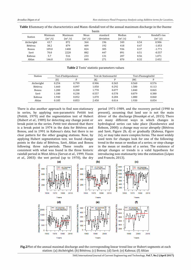
Table 1Summary of the characteristics and Mann–Kendall test of the annual maximum discharge in the Oueme

basin

Station Minimum

(m3 /s)

Maximum

(m3 /s)

Mean

(m3 /s)

standard

deviation

Median

(m3 /s) Cv

Kendall's tau

(m3 /y)

Atcherigbé 43.7 872 364 196 349 0.54 0.906

Bétérou 38.2 879 409 192 418 0.47 -1.053

Bonou 109.0 1400 824 305 936 0.37 -1.771

Savè 70.0 2220 882 447 891 0.51 -0.557

Kaboua 5.7 516 233 131 207 0.56 1.071

Ahlan 146.0 1310 849 271 870 0.32 2.452

Table 2 Tests’ statistic parameters values

Station Test d'Indépendance Test de Stationnarité Test d'homegénéité

|U| P |K| P |W| P

Atcherigbé 0.254 0.799 0.906 0.365 0.560 0.576

Bétérou 1.660 0.097 1.050 0.292 1.580 0.113

Bonou 1.280 0.200 1.770 0.077 1.840 0.065

Savè 1.180 0.238 0.557 0.578 0.879 0.380

Kaboua 1.940 0.052 1.070 0.284 1.880 0.060

Ahlan 0.185 0.853 2.450 0.014 1.930 0.054

There is also another approach to find non-stationary in series, by applying non-parametric Pettitt test (Pettitt, 1979) and the segmentation test of Hubert (Hubert et al., 1989) for detecting any change point or break point in the series. Pettit test showed that there is a break point in 1974 in the data for Bétérou and Bonou, and in 1991 in Kaboua’s data; but there is no clear pattern for the other gauging stations. Now, by applying Hubert segmentation test, we found change points in the data of Bétérou, Savè, Ahlan and Bonou following three sub-periods. These results are consistent with what was found in the three historic rainfall period in West Africa (Servat et al., 1999, Vissin et al., 2003): the wet period (up to 1970), the dry

period 1971–1989, and the recovery period (1990 to present), assuming that land use is not the main driver of the discharge (Hounkpè et al., 2015). There are many different ways in which changes in hydrological series can take place (Kundzewicz and Robson, 2000): a change may occur abruptly (Bétérou and Savè, Figure 2b, d) or gradually (Kaboua, Figure 2e), or may take more complex forms. The most widely used tests for changes look for one of the following: trend in the mean or median of a series; or step-change in the mean or median of a series. The existence of abrupt changes or trends is a valid hypothesis for introducing non-stationarity into the estimation (López and Francés, 2013).

Fig.2Plot of the annual maximal discharge and the corresponding linear trend line or Hubert segments at each station: (a) Atchérigbé; (b) Bétérou; (c) Bonou; (d) Savè; (e) Kaboua; (f) Ahlan



Table 3Correlation (significant at the 5% level) between Ouémé River annual maximum discharge series and climate indexes. The longitude and latitude are given for the SST (sea surface temperature) and SLP (sea level

pressure) grid cell

Stations Atchérigbé Bétérou Bonou Savè Kaboua Ahlan

SST

Period July July August Annual Average October January Longitude 156° 156° 156° 162° 138° 150° Latitude 104° 72° 72° 88° 68° 104°

Correlation coefficient 0.6 0.6 0.6 0.6 0.5 0.8 p-value 0.000032 0.000002 0.000002 0.000016 0.000148 0.000083

SLP

Period Annual Average Annual Average Annual Average August July April Longitude 156° 180° 180° 180° 144° 192° Latitude 108° 96° 96° 92° 108° 72°

Correlation coefficient 0.6 0.6 0.6 0.6 0.5 0.8 p-value < 8.10-06 < 4.10-07 < 10-06 < 10-05 <6.10-04 < 5.10-05

Table 4 Ouémé basin EOF’s results

Variance percentage

Station Atcherigbé Bétérou Bonou Savè Kaboua Ahlan PC1 45.30 40.00 46.34 41.42 41.24 43.09 PC2 18.56 21.15 19.82 19.19 19.31 15.95 PC3 15.25 14.88

14.73

Total 79.11 76.03 66.16 60.61 60.55 73.77

2.2. Covariates The inter relationship between the flood regime and climate indices that characterizes climate variability has recently been the subject of study worldwide. Many authors showed the influence of climate leading indices on flood regime. By realizing non-stationary flood frequency, they showed that distribution parameters could be function of climate indices and time (Aissaoui-Fqayeh et al., 2009, López and Francés, 2013, Hounkpè et al., 2015, Moss et al., 1994, Yang and Hill, 2012). Other study showed strong correlations between hydrologic quantiles and sub basin area (Avahounlin et al., 2013). There are many scientific debates on the covariates choice. Most of them used time and global climate indices such as North Atlantic Oscillation index (NAO), Arctic Oscillation index (AO), Mediterranean Oscillation index (MO), Southern Oscillation Index (SOI) and Western Mediterranean Oscillation index (WeMO) (Aissaoui-Fqayeh et al., 2009, López and Francés, 2013, Zhang et al., 2015, Coles and Davison, 2016, Vasiliades et al., 2015). Others preferred local covariates in addiction with climates indices, like land use change, altitude, reservoir index, local air temperature etc.(He et al., 2006, López and Francés, 2013, Tramblay et al., 2013, Musy and Meylan, 1987). In this study, we focused our attention on two climate indices: sea surface temperature (SST) and sea level pressure (SLP) anomalies. Among other regions, the Gulf of Guinea (GG) climate indexes: sea surface temperature (SST) and sea level pressure (SLP) (Mitchell, 2016); were found to be significantly well correlated at the 5% level with the observed data (Table 3). In fact, there is a well-known connection between the GG climate conditions and the West Africa

monsoon dynamics (and the associated precipitation) (Janicot et al., 2008). These indices were selected to incorporate climate forcings in non-stationary flood frequency analysis in Oueme River basin and acting as potential predictive variables. Temperature series such as interannualmaximas minimum Tminmax, mean Tmoymax and maximum Tmaxmax; and interannual minimums minimum Tminmin, mean Tmoymin and maximum Tmaxmin are also taken into account as predictive variables. Because there is lot of predictive variables and in order to simplify their use, this study proposes a prior EOFs analysis. EOFs analysis is similar to principal components analysis, but it is usually undertaken with two objectives: finding spatial patterns and reducing the dimensionality of a set of variables that reveal multi co-linearity. With the latter objective, it was decided to use this analysis because previous results have shown a high degree of correlation with climate indices that describe the behavior of macro scale atmospheric circulation patterns. EOFs analysis showed in Table 4, revealed that the first two or three principal components (PCs) with eigenvalue higher than one, account for more than 60 % of the total variance of the considered explanatory variables. Thus, it was decided to retain these two or three first PCs as explanatory covariates of the selected distribution parameters. The first principal component for Atchérigbé explanatory variables used (PC1 – 45 %) explains the temporal evolution of the interannual minimums temperature Tmoymin, Tmaxmin and Tminmin; while the second component (PC2 – 19 %) explains the inter annual maximums temperature Tminmax, Tmaxmax; and (PC3 – 15 %) is clearly linked to the evolution of SST and SLP anomalies.



The modeling period is 1952–2007 for the first four stations, whereas the time period 1960–2007 is used for Kaboua station and the time period 1986–2007 for Ahlan station. These are the common period for floods and climate indices records. These are the common period for floods and climate indices records. 2.3 Methodology Taking account of non-stationary for fitting time series with a distribution requires non-constant parameters for the distribution. Parameters laws assume here to be function of covariates or constant according to the optimized degrees of freedom. The “generalized additive models for location, scale and shape” (named GAMLSS), as proposed by Rigby and Stasinopoulos (Rigby and Stasinopoulos, 2005) is used here to reach this goal. Three models were used to realize the flood frequency analysis in a comparative goal. We got the stationary model (Model 0) where parameters are constant, the non-stationary model with time as covariate for parameters functions (Model 1) and the non-stationary with principal components (PC’s) as covariates for the parameters functions (Model 2). Generalized Additive Models for Location, Scale and Shape (GAMLSS) are semi-parametric regression-type models. A GAMLSS model assumes that, for independent observations have distribution function ( |

) where

( ) represents a vector of distribution parameters accounting for location, scale, and shape variables. The number of parameters is usually less than or equal to four, since one, two, three, and four parameter families can provide enough flexibility to model the data in hydrology. The distribution parameters are related to the design matrix of the selected covariates using the monotonic link function ( ) for . In this paper, only identity and logarithm link functions are used as the monotonic link functions. GAMLSS involves several models, and we used the semi-parametric additive formulation of GAMLSS given by:

( ) ∑ ( )

where are vectors with the length , is a matrix of explanatory variables (i.e., covariates) of order , is a parameter vector of length , and ( ) is used to represent the functional dependence of the distribution parameters on explanatory variables . This dependence can be linear or smooth through smoothing terms. Instead of assuming that the parameters are a linear function of explanatory variables, the smooth terms effect had already taken the linear dependence since the degrees of freedom could be equal to . The cubic spline function is the base of smooth terms. The smooth dependence between the explanatory variables and parameters tends to increase the complexity of the model. But to avoid model over-

fitting, the degrees of freedom are optimized using the Akaike Information Criterion (AIC) and the Schwarz Bayesian Criterion (SBC). For a more detailed discussion, readers can consult Rigby and Stasinopoulos (Rigby and Stasinopoulos, 2005). Final models are provided with a balance between accuracy and complexity. As tends to be zero, the cubic spline tends to a straight line. If there are no additive terms in any of the distribution parameters, the model can be given as follows:

( ) where is a combination of linear estimators. This form is the parametric linear model. If all the distribution parameters are independent of the covariates, then for , the model simplifies to a stationary model with constant parameters ( ) . Once we define the functional dependence between distribution parameters and each selected covariates and the effective degrees of freedom for the cubic spline, we select the distribution function ( |

)

according to the largest value of the maximum likelihood. In this paper, we considered as candidates five widely used distribution functions in modeling streamflow data (Table 5): Gumbel (GU); Lognormal (LNO); Weibull (WEI); Gamma (GA); and Generalized Gamma (GG). The first four have two parameters and the last one has three parameters. For a detailed discussion on theory, model fitting, and selection, the reader is referred to Rigby and Stasinopoulos (Rigby and Stasinopoulos, 2005, Stasinopoulos and Rigby, 2007) and Villariniet al. (Villarini et al., 2009b). In the absence of a statistic to evaluate the goodness of fit of the selected models as a whole, verification was made in accordance with the recommendations of Rigby and Stasinopoulos (Rigby and Stasinopoulos, 2005) by analyzing the normality and independence of the residuals of each model. Here, we checked the independence and normality of residuals by computing the first four statistical moments of the residuals and the Filliben correlation coefficients. Each statistical parameter was examined, and a visual inspection of diagnostic plots of the residuals (residuals vs. response, qq-plots and worm plots) was made. Worm plots are a de-trended representation of QQ plots, where indication about the agreement between the selected distribution and the data is provided by the shape of the ‘‘worm’’ (e.g., a flat ‘‘worm’’ supports the selection of the distribution). However, given the sampling uncertainties (in particular at the low and high quantiles), the points should lie within the 95 % confidence intervals. This action ensures that the selected models can adequately describe the systematic part, with the remaining information being random signal. To avoid over-fitting the model 2 according to external covariates selection and combination, we perform selection according to the procedure in (Rigby and Stasinopoulos, 2005). All of the calculations were performed on the platform R (R Development Core Team., 2008), using the freely available GAMLSS package.



Table 5Summary of the probability density function considered to model the annual maximum floods and the used link functions

Probability density function

Link functions g(.)

Gumbel

-

Lognormal

-

Weibull

-

Gamma

-

Generalized Gamma

Table 6Summary for the fitted models type 1 and the type of dependence between time and the distribution

parameters: cs(·) indicates the dependence is via the cubic splines with the indicated degree of freedom; without cs(·) means linear dependence; and ct refers to a parameter that is constant

Station Distribution Atcherigbé WEI t ct -

Bétérou GG cs(t, 5.16) t ct Bonou GG cs(t, 4.1) cs(t, 0.48) ct Savè GG cs(t, 2.26) cs(t, 1.83) ct

Kaboua GG cs(t, 1.84) t ct Ahlan GU t ct -

Table 7 Summary for the fitted models type 2, with the indication of the selected distribution, the significant covariates (PCs), and the type of dependence with the distribution parameters: cs(·) indicates the dependence is

via the cubic splines with the indicated degree of freedom; without cs(·) means linear dependence; and ct refers to a parameter that is independent of the covariates

Station Distribution

Atcherigbé GG PC2 + cs(PC3) PC3 ct Bétérou GU PC1 + PC2 ct - Bonou GU PC2 PC2 - Savè GG cs(PC2) PC2 ct

Kaboua GG PC1 + cs(PC2) PC2 ct Ahlan GU PC2 + PC3 ct -

3. Results 3.1 GAMLSS usage modeling This section presents the fitted non-stationary models (models 1 and 2) for the six study sites. Tables 6 and 7

produce the selected distributions as well as the type of dependence of distribution parameters as a function of time for model 1 and the selected distributions, the significant covariates for each parameter and the type of dependence of distributions parameters as a function of external covariates for model 2.

1 2 3

0,,

expexp1

,

21

2

1

2

1

2

21

y

yyyf y

()Identity ln()

0,0,0

2

logexp

1

2

1,

21

2

2

2

1

2

21

y

y

yyf y

()Identity ln()

0,0,0

exp,

21

11

1

221

2

2

y

yyyf y

ln() ln()

0,0,0

1

exp1

,

21

2

2

1

2

2

11

1

1

2

2

21

22

22

y

yy

yf y ln() ln()

0,0,,0

exp,,

321

223

1

1

321

1

31

31

y

yyyf y

ln() ln() ()Identity

1 2 3

1 2 3



First, it can be seen in both tables that the GG and GU distributions offer the best overall results in modeling the flood frequency in the Oueme basin even though the WEI distribution appears once. And second, the observed results show that temporal trends and external forcings can affect the behavior of the mean and the variance of the flood peak discharge. In all of the sites, the parameter includes time dependence and this dependence is generally via non-parametric smoothing functions (4 sites). The parameter is also usually time dependent except for two sites. There are just two cases with smooth dependence. For the sites in which the best fitted model was the GG distribution, the parameter is time independent in all cases. For the non-stationary models that incorporate external covariates (model 2), the high significance of PC2 is clear as shown by the explanatory covariate in the parameters of the selected distributions. It can also

be seen in Table 7 that PC2 is a significant covariate in parameter in all of sites, while it is a significant covariate for 3 sites for parameter . These results are due to the strong influence that the climates indices of the Gulf of Guinea (GG) climate indexes: sea surface temperature (SST) and sea level pressure (SLP) exert in modulating the hydroclimate in much of the basin. A weak statistical significance is observed for PC1, which is an explanatory covariate in 2 sites for the parameter and in no sites for the parameter. The lesser significance of PC1 is explained by the lesser influence of the local minima and maximas temperature series in modulating flood regimes, with nevertheless an influence limited to the annual maximas of maximum daily temperature Tmaxmax in all of sites (Table 8). It is supported by Figure 3. In a similar way to the results obtained in model 1, the parameter of the GG distribution is independent of climate covariates.

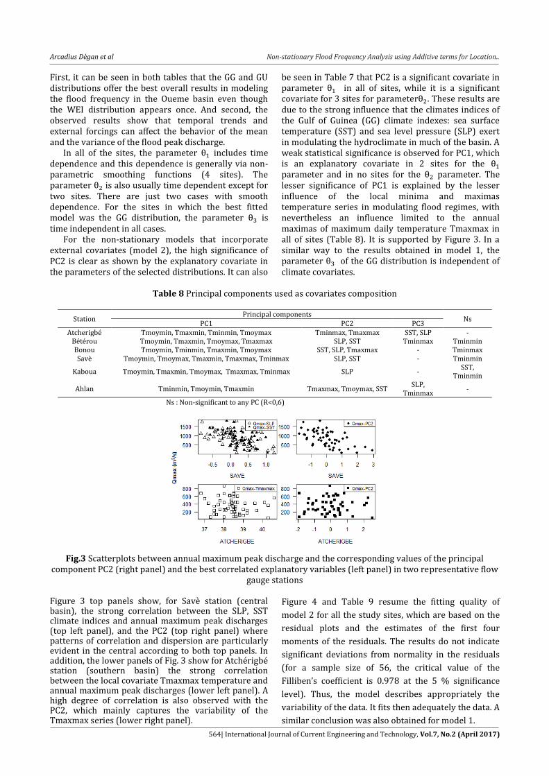
Table 8 Principal components used as covariates composition

Station Principal components

Ns PC1 PC2 PC3

Atcherigbé Tmoymin, Tmaxmin, Tminmin, Tmoymax Tminmax, Tmaxmax SST, SLP - Bétérou Tmoymin, Tmaxmin, Tmoymax, Tmaxmax SLP, SST Tminmax Tminmin Bonou Tmoymin, Tminmin, Tmaxmin, Tmoymax SST, SLP, Tmaxmax - Tminmax Savè Tmoymin, Tmoymax, Tmaxmin, Tmaxmax, Tminmax SLP, SST - Tminmin

Kaboua Tmoymin, Tmaxmin, Tmoymax, Tmaxmax, Tminmax SLP - SST,

Tminmin

Ahlan Tminmin, Tmoymin, Tmaxmin Tmaxmax, Tmoymax, SST SLP,

Tminmax -

Ns : Non-significant to any PC (R<0,6)

Fig.3 Scatterplots between annual maximum peak discharge and the corresponding values of the principal component PC2 (right panel) and the best correlated explanatory variables (left panel) in two representative flow

gauge stations Figure 3 top panels show, for Savè station (central basin), the strong correlation between the SLP, SST climate indices and annual maximum peak discharges (top left panel), and the PC2 (top right panel) where patterns of correlation and dispersion are particularly evident in the central according to both top panels. In addition, the lower panels of Fig. 3 show for Atchérigbé station (southern basin) the strong correlation between the local covariate Tmaxmax temperature and annual maximum peak discharges (lower left panel). A high degree of correlation is also observed with the PC2, which mainly captures the variability of the Tmaxmax series (lower right panel).

Figure 4 and Table 9 resume the fitting quality of

model 2 for all the study sites, which are based on the

residual plots and the estimates of the first four

moments of the residuals. The results do not indicate

significant deviations from normality in the residuals

(for a sample size of 56, the critical value of the

Filliben’s coefficient is 0.978 at the 5 % significance

level). Thus, the model describes appropriately the

variability of the data. It fits then adequately the data. A

similar conclusion was also obtained for model 1.



Fig.4 Worm plots of model 2 residuals for the sites stations. The two black dotted lines correspond to the 95% confident limits

Table 9 Residuals moments for model 2 and computed Filliben coefficient

Station Mean Variance Skewness Kurtosis Filliben coefficient

Atcherigbé 0.000 1.020 0.022 2.501 0.994 Bétérou 0.005 0.945 0.482 2.334 0.981 Bonou -0.001 1.014 0.028 2.757 0.995 Savè 0.000 1.019 0.098 2.419 0.995

Kaboua -0.005 1.006 0.121 2.130 0.989 Ahlan -0.008 1.093 -0.200 2.082 0.986

Fig.5 Summary of the results of modeling annual maximum peak discharge with models 1 and 2 under non stationary conditions. The results show the estimates of the median and the 2.5th and 97.5th percentiles

3.2 Non-stationary approaches results: comparison of Model 1 and Model 2

Figure 5 shows the observed values, the estimated median and the 2.5th and 97.5th percentiles for the six stations. The results obtained with non-stationary models, assuming temporal dependence only (model 1), show a pattern of decreasing trends in most of the

study sites, particularly during the post-1970 period, except in Atchérigbé and Ahlan, the two less long annual maximum discharge series; where they show an increase with a weak slope (0.51 m3/s/year and 10.94 m3/s/year respectively). Model 1 adequately describes the changes in annual maximum flood peaks such as an increasing tendency curve or a decreasing trend curve or a combination of both; however, time-trend models are unable to identify subsequent changes.



Table 10 Comparison of the AIC between the three models for the six stations

Station AIC

Model1-Model0 Model2-Model0 Model2-Model1 Model 0 Model 1 Model 2

Atcherigbé 748.0626 749.9732 724.7321 1.9106 -23.3305 -25.2411 Bétérou 744.8468 739.4253 708.4238 -5.4215 -36.423 -31.0015 Bonou 796.2703 783.2551 774.0347 -13.0152 -22.2356 -9.2204 Savè 834.8764 832.6268 816.989 -2.2496 -17.8874 -15.6378

Kaboua 601.4069 601.0781 565.9711 -0.3288 -35.4358 -35.107 Ahlan 304.8889 303.4527 291.3767 -1.4362 -13.5122 -12.076

3.3 Comparison between Stationary model and non-stationary models The study of floods in operational hydrology aims to

estimate flood events for a given exceedance

probability what is a priori chosen to obtain flooding

maps, design protective measures, and propose flood

risk management plans.

For a defined probability of exceedance, it is

possible to get the corresponding quantile for

stationary flood frequency analysis case. But here with

non-stationaries, it is noticed that this quantile is due

to the fitted value of the corresponding year and it is

obtained by the quantile function of the fitted model

with the parameters values of this year.

Considered significant period of return level are

generally between 2 and 3 , where is the number of

observations (here = 56). As for the various

hydrometric stations, a time series of 56 annual values

was established, return periods associated with

different laws will therefore be 2, 5, 10, 20, 50 and 100

years, 100 years being the representativeness limit.

But we have noticed there is not a large difference

(mean varying from 7.09 to 73.48) between the 50-

years quantiles and the 100-years one so we retain the

50-years quantile for models comparison.

Figure 6 shows the results of FFA in stationary

conditions (model 0) and non-stationary conditions

(models 1 and 2), for an exceedance probability of 0.02

(i.e. return period of 50 yr). Estimates are presented

for all the site stations.

The graphs highlight the problems of assuming

stationarity in estimating flood events. It can be seen

that non-stationarity models indicate the existence of

periods in which flood frequency experienced

significant variability (decreases and increases). We

can generally speak of a similar pattern of increases in

flood frequency during the periods 1960–1975 and

1995–2005. A clear decrease in flood frequency can be

seen during the period 1975–1995.

It is interesting to note that the non-stationarity

models indicate the existence of periods when the

flood risk experiences significant upward or downward

trends following different rainfall regimes. For

example, until the 1990s, there is a decreasing

flood risk, which may be due to the historical

droughts in the 1970s and the 1980s; after the 1990s,

there is a upward tendency with a weak Sen’s slope

estimator. In contrast, For Bonou there is a decrease

trend after 1990s for non-stationary model with time

varying and also for Atchérigbé and Ahlan, an increase

was observed during the entire study period. This was

already observed in the annual maximal discharge

series. Ahlan station case could be understood due to

its small data length, which starts from 1986.

These results suggest that an event-based design

assuming a stationary model can lead to two possible

major problems: considering greater or least risk or

over-sizing the structural and non-structural measures.

An FFA at Savè with model 2 shows that the peak flood

for an annual exceedance probability of 0.02 during the

56 years of the observation period ranges from a

maximum value of 1822.61 m3/s in 1995 to a low of

453 m3/s in 1982, while for the stationary case it is

constant (1654.98 m3/s). These values demonstrate

the big difference between considering stationary case

of flood frequency and the non-stationary. This

variation could lead to dramatic changes in the

structures’ sizing.

However, by considering maxima values records

out of the model 50-year value range, we noticed two

records for the stationary model: 1957’s and 1963’s

(1797 and 1734 respectively); one for non-stationary

with time varying model: 1963’s and finally one for

non-stationary with climates indices covariates model:

1957’s. For this one its maximum value covers this

record. Similar behaviour can be observed in all study

sites. These results strengthen the questioning

hypothesis of stationarity and lead us to suggest the

need for FFA that can take this dynamic behavior into

account while the stationary case is not so bad when

considering our time series.

Despite the good of fitness of the non-stationary

model which takes into account the dynamic behavior

of annual maximum discharge series, a feature point

should have more consideration. This concern the term

“return period” that loses meaning, as the probability

of excess changes from year to year. Therefore, in

complete agreement with (Hounkpè et al., 2015), new

definitions should be created by assuming the

hypothesis of non-stationarity(Olsen et al., 1998,

Sivapalan and Samuel, 2009, Salas and Obeysekera,

2013).



Fig.6Quantile estimates of the annual maximum floods with 0.02 annual exceedance probability for the period

1952–2007, based on models 0, 1 and 2

Fig.7 Results of modelling the annual maximum floods at Bétérou and Savè stations with models 1 and 2. Only the

period 1952–1993 is used for fitting the models (black circles and lines). The models are then used as predictive

tools (red lines) for the period 1994–2009/1994-2007 and observations not used in the fitting are shown with

blue circles

3.4 Non-stationary model as predictive tools To finalize the comparison of the two non-stationary models that are highlighted above, their predictive power is tested. Two flow gauges (Bétérou and Savè) were selected and their annual maximum discharge data are divided into three parts. The non-stationary models were fitted to first two-thirds: 1952-1993 and then we used the models as a predictive tool for the last third period: 1994-2009 or 1994-2010. The last two/three last years’ data were taken into account for

model 1 due to the time which is used for explanatory variable. The results shown in Figure 7 reveal the goodness of fit of the both models. For model 1, the curve follows a trend and was on an increasing trend after the 1990’s. In order to better judge this model, the period used for fitting should be extended to take into account the stabilized normal effect after the 1990’s before using its for prediction tool. For model 2, the changes in frequency of floods at the two sites are more accurately captured during the validation period where there was climate indices data. In order to use



model 2 as predictive tool, covariates data for this period must exist and available. This means that this model could only be used for a past period.

Conclusions

The flood frequency analysis under non-stationary conditions in the Ouémé basin at Bonou between the time period 1952 and 2007 was the main objective of the present study. The statistical modeling was conducted using GAMLSS models, which have the flexibility to deal with non-stationary probabilistic modeling, as well as the ability to model the dependence of distribution parameters with respect to external covariates (climate indices and local air temperature). Starting with the assumption of non-stationary data confirmed by Mann –Kendall test and the non-parametric Pettit test and Hubert segmentation, annual maximum discharge data showed a decreasing trend in most site stations according to the different rainfall regimes during the second half of the century over West Africa (Vissin E. W., 2001). The non-stationary modeling approaches used in GAMLSS showed that temporal trends and external forcings mostly affect the mean of the distributions, with much less effect on the variance. Although several mechanisms may be responsible for generating floods in the Ouémé river basin, this work showed that the climate indices Sea level Pressure (SLP) and Soil Surface Temperature (SST) indices, clearly are in close correlation with the genesis and concentration of precipitation that are causing floods, better than the local Temperature . By performing time-dependant parameters model, a non-linear dependency through parametric smoothing formulations is found and gives more goodness of fit than the linear function of the explanatory variable used. It can then obviously be validated that models that involve additive smooth terms by non-parametric cubic spline functions are more flexible and tend to better reproduce the dispersion of floods. However, the models which give the best goodness of fit and flexibility are the ones which remain sensitive to changes in evolution of predictive variables. Therefore, the explanatory variables choice had to be more specific and considered parsimoniously by using EOF analysis and then gives PC’s covariates, which are more sensitive with changes and the optimized degrees of freedom. Notably, according to the AIC criteria values obtained for each model; there is a high variation in the non-stationary model which uses the principal components based on the covariates variance and the ones using every covariate law or a combination law of them. These findings are an improvement compared with the work previously performed by Alamou(Alamou E., 2011), where all parameters were assumed to be constant and the work of Hounkpèet al. (Hounkpè et al., 2015), where only location parameter

is a linear combination of covariates and the others constant. An analysis of 50-year return period floods reveals that considering flood events as stationary leads to high uncertainties, and this can have two effects: underestimation of the flood risk or over-sizing of the flood design structures. The variations obtained are dramatic, with some periods where it is clearly seen that the flood quantile values are much higher than the estimates under stationary conditions. The weakness of non-stationary model is based on the term ‘’return-period’’ which concepts must be improved to not be so variable according to each specific year. An important discussion in this sense is the work presented recently by Salas and Obeysekera(Salas and Obeysekera, 2013). As perspective, structural measures remain important elements, and their designs should be updated by considering non-stationarity to reduce the vulnerability of human beings and goods exposed to flood risks. In addition, the non-stationary floods may be caused by climate change and urbanization, but only the climate indices and temperature were used in this study. Future studies will examine not only climate indices but also indices which can represent the human activities.

References AISSAOUI-FQAYEH, I., EL-ADLOUNI, S., OUARDA, T. B. M. J. &

ST-HILAIRE, A. 2009. Développement du modèle log-normal non-stationnaire et comparaison avec le modèle GEV non-stationnaire. Hydrological sciences journal, 54, 1141-1156.

Alamou, E. 2011. Application du Principe de Moindre Action à la modélisation pluie - Débit. . Thèse de Doctorat, , CIPMA Chaire Unesco FAST/UAC.

ALLEN, M. R. & SMITH, L. A. 1996. Monte Carlo SSA: Detecting irregular oscillations in the presence of colored noise. Journal of Climate, 9, 3373-3404.

AVAHOUNLIN, F. R., LAWIN, A. E., ALAMOU, E., CHABI, A. & AFOUDA, A. 2013. Analyse Fréquentielle des Séries de Pluies et Débits Maximaux de L’ ouémé et Estimation des Débits de Pointe. . Eur. J. Sci. Res. , 107, 355-369.

BROWN, S., CAESAR, J. & FERRO, C. A. 2008. Global changes in extreme daily temperature since 1950. Journal of Geophysical Research: Atmospheres, 113.

CHRISTOPH, M., FINK, A. H., PAETH, H., BORN, K., KERSCHGENS, M. & PIECHA, K. 2010. Climate scenarios ; . Impacts of global change on the hydrological cycle in West and Northwest Africa, pp. 402-425.

COLES, S. & DAVISON, A. 2016.Statistical Modelling of Extreme Values.

DELGADO, J. M., APEL, H. & MERZ, B. 2010. Flood trends and variability in the Mekong river. Hydrology and Earth System Sciences, 14, 407-418.

DOUGLAS, E. M., VOGEL, R. M. & KROLL, C. N. 2000. Trends in floods and low flows in the United States: impact of spatial correlation. Journal of hydrology, 240, 90-105.

EL ADLOUNI, S., OUARDA, T. B. M. J., ZHANG, X., ROY, R. & BOBÉE, B. 2007.Generalized maximum likelihood estimators for the nonstationary generalized extreme value model. Water Resour. Res, 43, W03410.



FRANKS & STEWART, W. 2002.Identification of a change in climate state using regional flood data.Hydrology and Earth System Sciences Discussions, 6, 11-16.

HASTIE, T. J. & TIBSHIRANI, R. J. 1990. Generalized additive models, CRC Press.

HE, Y., BÁRDOSSY, A. & BROMMUNDT, J. Non-stationary flood frequency analysis in southern Germany. Proceedings of the seventh international conference on hydroscience and engineering, Philadelphia, 2006.

HEJAZI, M. I. & MARKUS, M. 2009. Impacts of urbanization and climate variability on floods in northeastern Illinois.Journal of Hydrologic Engineering, 14, 606-616.

HELD, I. M. & SODEN, B. J. 2006.Robust responses of the hydrological cycle to global warming.Journal of Climate, 19, 5686-5699.

HOUNKPÈ, J., DIEKKRÜGER, B., BADOU, D. F. & AFOUDA, A. A. 2015.Non-stationary flood frequency analysis in the Ouémé River Basin, Benin Republic.Hydrology, 2, 210-229.

HUBERT, P., CARBONNEL, J. P. & CHAOUCHE, A. 1989. Segmentation des séries hydrométéorologiques—application à des séries de précipitations et de débits de l'Afrique de l'ouest. Journal of hydrology, 110, 349-367.

INTERGOVERNMENTAL PANEL FOR CLIMATE CHANGE.[IPCC], 2001. Climate Change 2001: Impacts, adaptation and vulnerability. Cambridge Univ. Press, New York.

ISHAK, E., RAHMAN, A., WESTRA, S., SHARMA, A. & KUCZERA, G. 2013.Evaluating the non-stationarity of Australian annual maximum flood.Journal of Hydrology, 494, 134-145.

JANICOT, S., THORNCROFT, C. D., ALI, A., ASENCIO, N., BERRY, G. J., BOCK, O., BOURLES, B., CANIAUX, G., CHAUVIN, F. & DEME, A. Large-scale overview of the summer monsoon over West Africa during the AMMA field experiment in 2006. AnnalesGeophysicae, 2008. 2569-2595.

KATZ, R. 1999. Extreme value theory for precipitation: sensitivity analysis for climate change. Advances in Water Resources, 23, 133-139.

KATZ, R. W., PARLANGE, M. B. & NAVEAU, P. 2002. Statistics of extremes in hydrology.Advances in water resources, 25, 1287-1304.

KENDALL, M. G. 1975. « Rank Correlation Methods" London, Charles Griffin.

KHALIQ, M. N., OUARDA, T., ONDO, J.-C., GACHON, P. & BOBÉE, B. 2006. Frequency analysis of a sequence of dependent and/or non-stationary hydro-meteorological observations: A review. Journal of hydrology, 329, 534-552.

KHARIN, V. V. & ZWIERS, F. W. 2005.Estimating extremes in transient climate change simulations.Journal of Climate, 18, 1156-1173.

KUNDZEWICZ, Z. & ROBSON, A. 2000.Detecting trend and other changes in hydrological data, World Meteorological Organization.

KWON, H. H., BROWN, C. & LALL, U. 2008. Climate informed flood frequency analysis and prediction in Montana using hierarchical Bayesian modeling. Geophysical Research Letters, 35.

LE BARBÉ, L., ALLÉ, G., MILLET, B., TEXIER, H., BOREL, Y. & GUALDE, R. 1993.Les ressources en eau superficielle de la république du Bénin. . Edition ORSTOM.

LECLERC, M. & OUARDA, T. B. M. J. 2007.Non-stationary regional flood frequency analysis at ungauged sites.Journal of Hydrology, 343, 254-265.

LÓPEZ, J. & FRANCÉS, F. Non-stationary flood frequency analysis in continental Spanish rivers, using climate and reservoir indices as external covariates. Hydrology and Earth System Sciences Discussions, 2013.European Geosciences Union (EGU), 3103-3142.

MCNEIL, A. J. & SALADIN, T. Developing scenarios for future extreme losses using the POT method.Embrechts, P.(Ed.), Extremes and Integrated Risk Management, 2000. Citeseer.

MILLY, PAUL, C. D., DUNNE, K. A. & VECCHIA, A. V. 2005.Global pattern of trends in streamflow and water availability in a changing climate.Nature, 438, 347-350.

MILLY, P. C. D., JULIO, B., MALIN, F., ROBERT, M., ZBIGNIEW, W., DENNIS, P. & RONALD, J. 2007.Stationarity is dead. Ground Water News & Views, 4, 6-8.

MITCHELL, T. 2016. 4 by 6-Degree Latititude-Longitude Resolution Anomalies of ICOADS SST, SLP, Surface Air Temperature, Winds, and Cloudiness. .

MOSS, M. E., PEARSON, C. P. & MCKERCHAR, A. I. 1994.The Southern Oscillation index as a predictor of the probability of low streamflows in New Zealand.Water Resources Research, 30, 2717-2723.

MUDELSEE, M., BÖRNGEN, M., TETZLAFF, G. & GRÜNEWALD, U. 2003. No upward trends in the occurrence of extreme floods in central Europe. Nature, 425, 166-169.

MUSY, A. & MEYLAN, P. 1987. Modélisation d'un processus non-stationnaire—Application à la pluviométrie en zone semi-aride. The Influence of Climatic Change and Climatic Variability on the Hydrologie Regime and Water Resources, 287-299.

OLSEN, J. R., LAMBERT, J. H. & HAIMES, Y. Y. 1998.Risk of extreme events under nonstationary conditions.Risk Analysis, 18, 497-510.

OUARDA, T. B. M. J. & EL‐ADLOUNI, S. 2011. Bayesian nonstationary frequency analysis of hydrological variables1.Wiley Online Library.

PETTITT, A. 1979.A non-parametric approach to the change-point problem.Applied statistics, 126-135.

RENARD, B., LANG, M. & BOIS, P. 2006. Statistical analysis of extreme events in a non-stationary context via a Bayesian framework: case study with peak-over-threshold data. Stochastic environmental research and risk assessment, 21, 97-112.

RIGBY, R. A. & STASINOPOULOS, D. M. 2005. Generalized additive models for location, scale and shape.Journal of the Royal Statistical Society: Series C (Applied Statistics), 54, 507-554.

ROBSON, A. J., JONES, T. K., REED, D. W. & BAYLISS, A. C. 1998.A study of national trend and variation in UK floods.International Journal of Climatology, 18, 165-182.

SALAS, J. D. & OBEYSEKERA, J. 2013. Revisiting the concepts of return period and risk for nonstationary hydrologic extreme events.Journal of Hydrologic Engineering, 19, 554-568.

SANKARASUBRAMANIAN, A. & LALL, U. 2003. Flood quantiles in a changing climate: Seasonal forecasts and causal relations. Water Resources Research, 39.

SEIDOU, O., RAMSAY, A. & NISTOR, I. 2012. Climate change impacts on extreme floods II: improving flood future peaks simulation using non-stationary frequency analysis. Natural hazards, 60, 715-726.

SERVAT, E., PATUREL, J., LUBÈS-NIEL, H., KOUAMÉ, B., MASSON, J., TRAVAGLIO, M. & MARIEU, B. 1999. De différents aspects de la variabilité de la pluviométrie en Afrique de l'Ouest et Centrale non sahélienne. Revue des sciences de l'eau/Journal of Water Science, 12, 363-387.

SIVAPALAN, M. & SAMUEL, J. M. 2009. Transcending limitations of stationarity and the return period: process‐based approach to flood estimation and risk assessment.Hydrological processes, 23, 1671-1675.

SPETH, P., CHRISTOPH, M. & DIEKKRÜGER, B. 2010.Impacts of global change on the hydrological cycle in West and Northwest Africa, Springer Science & Business Media.



STASINOPOULOS, D. M. & RIGBY, R. A. 2007. Generalized additive models for location scale and shape (GAMLSS) in R. Journal of Statistical Software, 23, 1-46.

STEDINGER & JERY R 1993.Frequency analysis of extreme events.Handbook of hydrology, 18.

STEDINGER, J. R. & CRAINICEANU, C. M. 2000.Climate variability and flood-risk management.Risk-based decision making in water resources IX, 77-86.

STRUPCZEWSKI, W. G., SINGH, V. P. & MITOSEK, H. T. 2001. Non-stationary approach to at-site flood frequency modelling. III. Flood analysis of Polish rivers. Journal of Hydrology, 248, 152-167.

R Development Core Team, 2008. R: A Language and Environment for Statistical Computing; . R Foundation for Statistical Computing: .

TRAMBLAY, Y., NEPPEL, L., CARREAU, J. & NAJIB, K. 2013.Non-stationary frequency analysis of heavy rainfall events in southern France.Hydrological Sciences Journal, 58, 280-294.

VASILIADES, L., GALIATSATOU, P. & LOUKAS, A. 2015. Nonstationary frequency analysis of annual maximum rainfall using climate covariates.Water Resources Management, 29, 339-358.

VILLARINI, G., SERINALDI, F., SMITH, J. A. & KRAJEWSKI, W. F. 2009a.On the stationarity of annual flood peaks in the continental United States during the 20th century.Water Resources Research, 45.

VILLARINI, G., SMITH, J. A. & NAPOLITANO, F. 2010. Nonstationary modeling of a long record of rainfall and temperature over Rome.Advances in Water Resources, 33, 1256-1267.

VILLARINI, G., SMITH, J. A., SERINALDI, F., BALES, J., BATES, P. D. & KRAJEWSKI, W. F. 2009b.Flood frequency analysis for nonstationary annual peak records in an urban drainage basin.Advances in Water Resources, 32, 1255-1266.

VISSIN, E., BOKO, M., PERARD, J. & HOUNDENOU, C. 2003.Recherche de ruptures dans les séries pluviométriques et hydrologiques du bassin béninois du fleuve Niger (Bénin, Afrique de l'Ouest). Publications de l’Association Internationale de Climatologie, 368-376.

VISSIN E. W. 2001. Contribution à l’étude de la variabilité des précipitations et des écoulements dans le bassin béninois du fleuve Niger. . Mémoire de DEA, Université de Bourgogne.

VOGEL, R. M., YAINDL, C. & WALTER, M.

2011.Nonstationarity: Flood magnification and recurrence

reduction factors in the United States1. Wiley Online

Library.

WALD, A. & WOLFOWITZ, J. 1943.An exact test for

randomness in the non-parametric case based on serial

correlation.The Annals of Mathematical Statistics, 14, 378-

388.

WILCOXON, F. 1945. Individual comparisons by ranking

methods.Biometrics bulletin, 1, 80-83.

WILSON, D., HISDAL, H. & LAWRENCE, D. 2010. Has

streamflow changed in the Nordic countries?–Recent

trends and comparisons to hydrological projections.

Journal of Hydrology, 394, 334-346.

XIONG, L. & GUO, S. 2004. Trend test and change-point

detection for the annualdischargeseries of the Yangtze

River at the Yichang hydrological station/Test de tendance

et détection de rupture appliqués aux séries de débit

annuel du fleuve Yangtze à la station hydrologique de

Yichang. Hydrological Sciences Journal, 49, 99-112.

YANG, C. & HILL, D. 2012.Modeling Stream Flow Extremes

under Non-Time-Stationary Conditions.

YEE, T. W. & STEPHENSON, A. G. 2007. Vector generalized

linear and additive extreme value models. Extremes, 10, 1-

19.

ZHANG, D.-D., YAN, D.-H., WANG, Y.-C., LU, F. & LIU, S.-H.

2015. GAMLSS-based nonstationary modeling of extreme

precipitation in Beijing–Tianjin–Hebei region of China.

Natural Hazards, 77, 1037-1053.

ZHANG, X., HARVEY, K. D., HOGG, W. & YUZYK, T. R.

2001.Trends in Canadian streamflow.Water Resources

Research, 37, 987-998.

ZVERYAEV, I. I. 2000. DECADE‐TO‐CENTURY‐SCALE

CLIMATE VARIABILITY AND CHANGE: A SCIENCE

STRATEGY. Panel on Climate Variability on Decade‐to‐

Century Time Scales, Board on Atmospheric Sciences and

Climate, Commission on Geosciences, Environment, and

Resources, National Research Council, National Academy

Press, Washington, DC, 1998. No. of pages: xii+ 142. Price£

27.95. ISBN 0‐309‐06098‐2.International Journal of

Climatology, 20, 933-933.

non-stationary flood frequency analysis using additive...

Documents