nonlinear elasticity with applications to the arterial

A. M. Robertson, Nonlinear elasticity, Spring 2009 1

Supplementary Notes for:

Nonlinear elasticity with applications to the arterial wall

Short Course in the

EU-Regional School in Computational Engineering Science

RWTH Aachen University

Part I- March 27, 2009

Part II- April 3, 2009

Associate Professor A. M. RobertsonDepartment of Mechanical Engineering and Materials ScienceMcGowan Institute for Regenerative MedicineCenter for Vascular Remodeling and Regeneration (CVRR)University of Pittsburgh

2 A. M. Robertson, Supplementary Notes

Contents

1 Kinematics 71.1 Continuum Idealization . . . . . . . . . . . . . . . . . . . . . . . . . . . . . 71.2 Description of motion of material points in a body . . . . . . . . . . . . . . 71.3 Referential and spatial descriptions . . . . . . . . . . . . . . . . . . . . . . . 91.4 Displacement, Velocity, and Acceleration . . . . . . . . . . . . . . . . . . . . 10

1.4.1 Displacement . . . . . . . . . . . . . . . . . . . . . . . . . . . . . . . 101.4.2 Velocity and Acceleration . . . . . . . . . . . . . . . . . . . . . . . . 10

1.5 Deformation Gradient of the Motion . . . . . . . . . . . . . . . . . . . . . . 111.6 Transformations of infinitesimal areas and volumes during the deformation 13

1.6.1 Transformation of infinitesimal areas . . . . . . . . . . . . . . . . . . 131.6.2 Transformation of infinitesimal volumes . . . . . . . . . . . . . . . . 13

1.7 Measures of Stretch and Strain . . . . . . . . . . . . . . . . . . . . . . . . . 141.7.1 Material stretch and strain tensors, C and E . . . . . . . . . . . . . 141.7.2 Spatial Stretch and Strain Tensors, b, e . . . . . . . . . . . . . . . . . 16

1.8 Polar Decomposition of the Deformation Gradient Tensor . . . . . . . . . . 171.9 Other Strain Measures . . . . . . . . . . . . . . . . . . . . . . . . . . . . . . 191.10 Velocity Gradient . . . . . . . . . . . . . . . . . . . . . . . . . . . . . . . . . 19

1.10.1 Vorticity Vector and Vorticity Tensor . . . . . . . . . . . . . . . . . 221.11 Special Motions . . . . . . . . . . . . . . . . . . . . . . . . . . . . . . . . . . 22

1.11.1 Isochoric Motions . . . . . . . . . . . . . . . . . . . . . . . . . . . . . 221.11.2 Irrotational Motions . . . . . . . . . . . . . . . . . . . . . . . . . . . 221.11.3 Homogeneous Deformations . . . . . . . . . . . . . . . . . . . . . . . 221.11.4 Rigid Motions . . . . . . . . . . . . . . . . . . . . . . . . . . . . . . . 231.11.5 Pure Homogeneous Deformation . . . . . . . . . . . . . . . . . . . . 241.11.6 Plane Strain . . . . . . . . . . . . . . . . . . . . . . . . . . . . . . . 241.11.7 Axisymmetric Strain . . . . . . . . . . . . . . . . . . . . . . . . . . . 251.11.8 Non-Homogeneous Deformations . . . . . . . . . . . . . . . . . . . . 28

2 Governing Equations 292.1 Governing Equations . . . . . . . . . . . . . . . . . . . . . . . . . . . . . . . 29

2.1.1 Conservation of Mass . . . . . . . . . . . . . . . . . . . . . . . . . . 302.1.2 Balance of Linear Momentum . . . . . . . . . . . . . . . . . . . . . . 32

3


2.1.3 Balance of Angular Momentum . . . . . . . . . . . . . . . . . . . . . 352.1.4 Mechanical Energy Equation . . . . . . . . . . . . . . . . . . . . . . 362.1.5 Balance of Energy . . . . . . . . . . . . . . . . . . . . . . . . . . . . 372.1.6 Clausius-Duhem Inequality . . . . . . . . . . . . . . . . . . . . . . . 392.1.7 Summary of Governing Equations: . . . . . . . . . . . . . . . . . . . 40

2.2 Constraints . . . . . . . . . . . . . . . . . . . . . . . . . . . . . . . . . . . . 412.2.1 Incompressible materials - constraint of incompressibility . . . . . . 412.2.2 Inextensible Fibers - constraint of inextensibility . . . . . . . . . . . 42

3 Constitutive Equations 433.1 Restrictions on the Stress Tensor . . . . . . . . . . . . . . . . . . . . . . . . 43

3.1.1 Superposed Rigid Body Motion . . . . . . . . . . . . . . . . . . . . . 463.2 Nonlinear Elastic Material (Cauchy-Elastic Material) . . . . . . . . . . . . . 50

3.2.1 Implications of invariance under a superposed rigid body motion . . 513.3 Viscous fluids . . . . . . . . . . . . . . . . . . . . . . . . . . . . . . . . . . . 51

3.3.1 Compressible Newtonian Fluid . . . . . . . . . . . . . . . . . . . . . 533.3.2 Ideal Fluid . . . . . . . . . . . . . . . . . . . . . . . . . . . . . . . . 53

3.4 Hyperelastic Materials . . . . . . . . . . . . . . . . . . . . . . . . . . . . . . 533.4.1 Relationship between W and the Helmholtz free energy . . . . . . . 553.4.2 Invariance restrictions . . . . . . . . . . . . . . . . . . . . . . . . . . 55

3.5 Materials with Symmetry . . . . . . . . . . . . . . . . . . . . . . . . . . . . 563.5.1 Isotropic hyperelastic materials . . . . . . . . . . . . . . . . . . . . . 573.5.2 Transversely Isotropic Materials . . . . . . . . . . . . . . . . . . . . 60

3.6 Finite Elastic Constitutive Equation for Fiber-Reinforced Material . . . . . 613.6.1 Constitutive Equation for One Family of Fibers . . . . . . . . . . . . 613.6.2 Kinematics . . . . . . . . . . . . . . . . . . . . . . . . . . . . . . . . 623.6.3 Finite Elasticity for Two Families of Fibers . . . . . . . . . . . . . . 65

A Additional Considerations for SRBM 69

B Isotropic Tensors 73

C Isotropic Tensor Functions 77C.1 Scalar valued isotropic tensor functions . . . . . . . . . . . . . . . . . . . . . 77C.2 Symmetric Isotropic Tensor Functions . . . . . . . . . . . . . . . . . . . . . 78

D Some Derivations for Isotropic Materials 79D.0.1 Results for the invariants for second order tensors C and a0 ⊗ a0 . . 80D.0.2 Results for the invariants for second order tensors C, a0 ⊗ a0, g

0⊗ g

080

Notation


Before proceeding further, we discuss some of the notation used in this chapter. We makeuse of Cartesian coordinates and the standard Einstein summation convention. For clarity,relations are often given in both coordinate free notation as well as component form.

In general, lower case letters (Greek and Latin) are used for scalar quantities, boldfacelowercase letters are used for first order tensors (vectors) and boldface upper case letters areused for second order tensors. The components of tensors relative to fixed orthonormal basis(rectilinear) (e1, e2, e3) are denoted using Latin subscripts. Standard summation conventionis used whereby repeated Latin indices imply summation from one to three. The innerproduct between two arbitrary vectors u and v is denoted using the “·” notation and definedin this chapter as,

u · v = ui vi. (1)

The linear transformation formed by the operation of a second order tensor A on a vectoru to generate a vector v is written as v = Au 1. The product of two second order tensorsAB generates another second order tensor C,

C = AB or Cij = Aik Bkj . (2)

The inner product of two second order tensors A and B is denoted by A : B and defined as,

A : B = trace(AT B) or A : B = Aij Bij . (3)

1Some texts write v = Au.

Chapter 1

Kinematics

1.1 Continuum Idealization

In this class, we consider the bulk response of materials, rather than focusing on the behaviorat the microscopic level. In doing so, we will make use of a continuum mechanics model inwhich we assume that the physical body under analysis completely fills a region in physicalspace. Namely, we idealize a physical body, B, as being composed of a continuous set ofmaterial points (or continuum particles).

1.2 Description of motion of material points in a body

In order to identify these material points within the body and describe the motion/deformationof the body, we embed B in a three-dimensional Euclidean space, Figure 1.2. As the bodydeforms (moves) in time, it will occupy different regions in space. We call these regionsconfigurations and denote the configuration at an arbitrary current time t by κ(t). Thisconfiguration will be referred to as the current configuration. We choose a particular con-figuration of B to serve as a reference configuration, enabling us to uniquely identify anarbitrary material point P in B by its position X in this configuration. We denote thisspecial configuration as κ0

1. For example, κ0 could be the configuration of the body attime zero, though it is not necessary that the configuration of the body have ever coincidedwith reference configuration κ0.

During the deformation (or motion) of B, an arbitrary material particle P located atposition X in reference configuration κ0 will move to position x in configuration κ(t). Thevector X is sometimes referred to as the referential position and x as the current positionof the material point P

It is assumed that the motion of this arbitrary material point in B can be described

1The use of the upper case symbol for the position vector in κ0 is an exception to the notation for vectorsintroduced above.

7


Figure 1.1: Schematic of notation used to identify material points and regions in an arbitrarybody B in the reference configuration κ0 and current configuration κ(t).

through a relationship of the form

x = χ(X, t) for t ≥ 0. (1.1)

With respect to the map given in (1.1), we will make the following mathematical assump-tions:

1. The function χκ0

(X, t) is continuously differentiable in all variables, at least upthrough the second derivatives.

2. At each fixed time t ≥ 0, the following property holds: for any X and correspondingx, there are open balls BX (centered at X) and Bx (centered at x), both containedin B, such that points of BX are in one-to-one correspondence with points of Bx.

These mathematical assumptions correspond to specific physical requirements. The firstensures a degree of smoothness of the trajectories of material points that will allow us todefine quantities such as the velocity and acceleration. The second assumption implies thefollowing two conditions are met:

• Impenetrability of the body

• No voids are created in the body.

The second condition also implies that the Jacobian J of the transformation (1.1) is non-zeroat all times t ≥ 0 and all points in the body. Here, J is

J = det

(∂χ

κ0(X, t)

∂X

). (1.2)


If the reference configuration of the body was at any time t∗ an actual configuration of thebody, then at this time, x = X. At this time, it follows that J(t∗) = 1. However, as juststated, J can never vanish, so that if J is positive at one time, it must be positive at alltimes. We can therefore, conclude that under these conditions, for all points in the body,

J > 0, for all t ≥ 0. (1.3)

Furthermore, we can conclude that the transformation (1.1) posseses and inverse,

X = χ−1(x, t). (1.4)

For future discussions, it will be useful to introduce notation for identifying variousregions of the body. The region occupied by the entire body in κ0 will be denoted by R0

with closed boundary ∂R0, Figure 1.2. The corresponding regions and boundaries for thebody in κ(t) are R and ∂R, respectively. An arbitrary material region within B in κ0 will bedenoted as V0 (V0 ⊆ R0) with boundary ∂V0. The corresponding subregion in the currentconfiguration κ(t) will be denoted as V (V ⊆ R) with boundary ∂V.

For the current purposes, it suffices to define one reference configuration for the body.Hence, in further discussions, we drop the subscript κ0 and it will be understood that thefunctions χ(X, t) and χ−1(x, t) depend on the choice of reference configuration. However, infuture discussion of multi-mechanism materials, more than one reference configuration willbe employed. In these discussions, we will make use of subscripts of this kind to identifythe appropriate reference configuration.

1.3 Referential and spatial descriptions

It follows from the second mathematical assumption that the vectors X and x for a materialpoint P are in one-to-one correspondence. Therefore, field variables such as the density, ρ,can either be written as a function of X and t (the referential or Lagrangian description)or as a function of x and t, (the spatial or Eulerian description),

ρ = ρ(X, t) = ρ(x, t). (1.5)

Clearly these two descriptions can be related using (1.1) and (1.4),

ρ(x, t) = ρ(χ(X, t), t) ≡ ρ(X, t) (1.6)

andρ(X, t) = ρ(χ−1(x, t), t) ≡ ρ(x, t) (1.7)

The Eulerian description ρ(x, t) is independent of information about the position of indi-vidual material particles and is typically used for the motion of viscous fluids.

When discussing entities such as the gradient, divergence or curl that involve spatialderivatives, we need to be clear whether we are considering these quantities in terms ofposition vector in the referential or current configuration. It will be convenient to use


capital letters/lower case letters when we use the referential/current spatial variable. Forexample, for a field variable f = f(X, t) = f(x, t),

Gradf =∂f(X, t)∂X

and gradf =∂f(x, t)∂x

. (1.8)

1.4 Displacement, Velocity, and Acceleration

1.4.1 Displacement

The displacement u of a particle P at time t is defined by,

u = x − X. (1.9)

In writing (1.9), we have not specified how we are evaluating the right hand side of equation.In particular, if we make use of (1.1), we obtain the displacement in Eulerian form,

u(x, t) = x − χ−1(x, t). (1.10)

Alternatively, using (1.4), we obtain the Lagrangian description,

u(X, t) = χ(X, t) − X. (1.11)

1.4.2 Velocity and Acceleration

The velocity v of a material point P is defined as the time derivative of the displacement(1.11) (for fixed material particle),

v =∂u(X, t)

∂tor v =

∂χ(X, t)∂t

, (1.12)

The acceleration of the same particle P is defined as the time derivative of the velocity, (forfixed material particle),

a =∂v(X, t)

∂t=

∂2χ(X, t)

∂t2. (1.13)

As was done for the density field, both these field variables can be written in Eulerian formusing (1.4). For example,

v = v(X, t) = v(χ−1(x, t), t) = v(x, t). (1.14)

Material DerivativeThe material derivative of a field variable such as density, is defined as the partial derivativeof the function with respect to time holding the material point fixed,

Dρ

Dt=

∂ρ(X, t)∂t

. (1.15)


Sometimes the material derivative is called the total derivative or substantial derivative. Forexample, it follows that the acceleration is the material derivative of the velocity field.

Frequently in fluid mechanics we work with the Eulerian representation of functionswithout knowledge of the deformation (1.1) with which to obtain the Lagrangian represen-tation from the Eulerian representation. As a result, it is not possible to directly evaluate(1.15). Using the chain rule, the material derivative can be written for the spatial formula-tion of a field variable. For example, in the case of the density field,

Dρ

Dt=

∂ρ(x, t)∂t

+ vi∂ρ(x, t)∂xi

orDρ

Dt=

∂ρ(x, t)∂t

+ v(x, t) · gradρ(x, t). (1.16)

Therefore, depending on the representation we have for a field variable, we have two choicesfor the material derivative. Once again, for a scalar field variable,�

�

�

�

Material Derivative

Dρ

Dt=

⎧⎪⎪⎨⎪⎪⎩

∂ρ(X, t)∂t

Lagrangian Representation

∂ρ(x, t)∂t

+ v(x, t) · gradρ(x, t) Eulerian Representation

(1.17)

Using (1.17), we may obtain the acceleration from the spatial representation of the velocityfield,

a =∂v(x, t)∂t

+ (gradv(x, t))v(x, t) or ai =∂vi(x, t)∂t

+∂vi(x, t)∂xj

vj. (1.18)

In summary, we can calculate the acceleration from either the Lagrangian or Eulerianrepresentation of the velocity vector using (1.13) or (1.18),�

�

�

�

Acceleration

a =

⎧⎪⎪⎨⎪⎪⎩

∂v(X, t)∂t

∂v(x, t)∂t

+ (gradv(x, t)) v(x, t)

(1.19)

1.5 Deformation Gradient of the Motion

Let x be the position of a material point P in κ and y be the position of another particle Qin the neighborhood N of P . We assume N is very small so that y − x is an infinitesimalvector. The rectangular components of dxi = (dx1, dx2, dx3). It can then be shown from(1.1), that

dxi =∂χi(x, t)∂XA

dXA. (1.20)


It is straightforward to prove the components ∂χi/∂XA, (i, A = 1, 2, 3) transform under achange of basis like the components of a second order tensor. We denote this tensor as F ,so that, �

�

�

�

Deformation Gradient Tensor:

F ≡ ∂χ(X, t)∂X

or FiA =∂χi(X, t)∂XA

.

and

Inverse Deformation Gradient Tensor:

F−1 ≡ ∂χ−1(x, t)∂x

or F−1Ai =

∂χ−1A (x, t)∂xi

.

(1.21)

Using this notation, it follows from (1.20),

�� dx = F dX, or dxi = FiAdXA. (1.22)

It is clear from this last expression, that F determines how infinitesimal vectors in the

Figure 1.2: Deformation of an infinitesimal material element,dX in κ0 which is transformed to dx in κ(t).

reference configuration are deformed (stretched and rotated) during the motion, Fig. 1.3.For this reason, F is called the deformation gradient tensor. Using the notations introducedin (1.8) with (1.10) and (1.11), we see that F and F−1 are related to the gradients of thedisplacement vector through

F = Gradu + I, F−1 = I − gradu. (1.23)


1.6 Transformations of infinitesimal areas and volumes dur-

ing the deformation

The transformation of an infinitesimal material element dX from the reference configurationto the current configuration is determined through F . This tensorial relationship can inturn be used to calculate the changes in material area and volume during the deformation.

1.6.1 Transformation of infinitesimal areas

If we consider two distinct infinitesimal material line elements dY , dZ in configuration κ0

at X, then we may define an infinitesimal material area dA in κ0 and the correspondingarea da in κ(t)

dA ≡ dY × dZ, da ≡ dy × dz, (1.24)

where dA can be written as the product of its magnitude dA and unit normal N such thatdA = NdA. Similarly, da = nda in κ(t), where n is the unit normal and da is the magnitudeof area da. Noting from (1.22) that dy ≡ F dY and dz ≡ F dZ , it then follows,

dam = εmjk FjB FkC dYBdZC

= εijk δim FjB FkC dYBdZC

= εijk FiA F−1Am FjB FkC dYBdZC

= εABC J F−1Am dYBdZC

= J F−1AmdAA

(1.25)

Namely, we have Nanson’s formula,�� Nanson’s Formula: da = JF−T dA. (1.26)

1.6.2 Transformation of infinitesimal volumes

If we consider three distinct material non-planar line elements dX, dY , dZ in configurationκ0 at X , then we may define an infinitesimal material volume dV in κ0 with volume dv inκ(t) as,

dV ≡ dX · (dY × dZ), dv ≡ dx · (dy × dz), (1.27)

where dx ≡ F dX, dy ≡ F dY and dz ≡ F dZ . It then follows that,

dv = εijk FiA FjB FkC dXA dYB dZC

= εABC JdXA dYB dZC (1.28)

and therefore, �� dv = J dV. (1.29)


Note, that in obtaining (1.26) and (1.28), we have made use of the following result for asecond order tensor, A,

εijkdetA = εlmn AliAmj Ank. (1.30)

It will be useful in the discussion of the governing equations to note the following result forthe material derivative of the Jacobian of the transformation (1.1),

DJ

Dt= J div v, (1.31)

where v is the velocity vector.

1.7 Measures of Stretch and Strain

In the last section, we discussed the deformation gradient tensor, which completely de-termines the mapping of an infinitesimal material element from the reference to currentconfiguration. In this section, we consider specific characteristics of this mapping. In par-ticular, we consider the stretch and strain undergone by this material element. Unlike thedeformation gradient, which has a unique definition, the strain of an infinitesimal materialelement can be defined in a number of ways.

1.7.1 Material stretch and strain tensors, C and E

We first consider an infinitesimal material element dX = a0dS in the κ0 which is mappedto dx = a ds in κ(t) where a0 and a are unit vectors, Figure 1.3. The stretch undergone bythis material element during the deformation is defined as λ ≡ |dx|/|dX| = ds/dS. Using(1.22), we can rewrite magnitude of the infinitesimal vector dx as follows,

ds2 = |dx|2 = dx · dx = a0 · (FTF a0)dS2 (1.32)

Recalling the definition of the right Cauchy-Green tensor (sometimes called the Green de-formation tensor)�� Right Cauchy-Green Tensor: C ≡ FTF, or CAB ≡ FiA FiB , (1.33)

we therefore have from (1.32), �� λ2 = a0 ·C a0. (1.34)

Namely, the stretch of a material element located at X in κ0, can be calculated at arbitrarytime t solely from knowledge of its orientation in κ0 and the tensor C at X at time t.

It can be shown that, for all material points in the body at all times, C is symmetricand positive definite

u · (C u) > 0 for all u �= 0. (1.35)

The proof of symmetry follows directly from the definition (1.33)

CT = (F TF )T = FTF = C, (1.36)


Physical Significance of Diagonal Elements of C

Consider at infinitesimal element represented by dX in the reference configuration and dx

in the current configuration. If we now consider the special case where dX = dSe1, then itfollows from (1.34), that

ds2

dS2 = C11. (1.37)

The ratio ds2/dS2 is typically called the stretch ratio and denoted by λ. We can describethe result (1.37) in words as,�

� C11 is equal to the stretch ratio squared of an infinitesimal material element

was aligned with the e1 axis in the reference configuration.

More generally, the diagonal elements of C have a specific physical meaning. Cii (no sumon i) is the square of the stretch of a material element which was aligned with the directionei in κ0.

Physical significance of off-diagonal elements of C

Now consider two infinitesimal material elements corresponding to dX(1) = dS(1)a(1)0 and

dX(2) = dS(2)a(2)0 . where a(1)

0 and a(2)0 are unit vectors. In the current configurations, these

infinitesimal elements are denoted as dx(1) = ds(1)a(1) and dx(2) = ds(2)a(2), respectively.The angle between these same material elements in the current configuration will be denotedas α. Therefore,

cosα =dx · dxds(1)ds(2)

=FiAFiBa

(1)0Aa

(1)0BdS(1)dS(2)

ds(1)ds(2)=

CABa(1)0Aa

(1)0B

λ(1) λ(2). (1.38)

Now consider the special case, where the infinitesimal elements are perpendicular in thereference configuration, for example, a(1)

0 = e1 and a(2)0 = e2, in which case, (1.38) reduces

to,

cosα =C12√C11C22

. (1.39)

For example, if the angle between the elements remains unchanged (still 90o), then C12 = 0.If the angle decreases from 90o, then C12 will be a positive number. If the α ∈ (90o, 270o),then C12 will be negative.

Lagrangian Strain

In addition, to considering the stretch of an infinitesimal material element, it is of interest tostudy its strain. While there is no unique definition, one measure of interest is the change inthe square of the magnitude of the infinitesimal material element, relative to its magnitude


squared in κ0. This strain measure can be related to the right Cauchy-Green tensor using(1.34),

ds2 − dS2

dS2= (λ2 − 1) = a0 · (C − I) a0. (1.40)

The quantity in brackets is twice the Green-Lagrange Strain Tensor��

��Green-Lagrange Strain Tensor: E ≡ 1

2(C − I). (1.41)

The motivation for the factor of one-half in this definition will become clear when linearelasticity is considered. It therefore follows from (1.40) and (1.41) that,

�� 1

2ds2 − dS2

dS2 = a0 · E a0. (1.42)

From (1.41), we see that the diagonal components of E have physical significance. Eii (nosum on i) is the strain undergone by a material element which is tangent to ei in κ0. Thestrain is taken relative to dS, the length of this element in κ0. Using the definition of thestrain tensors with (1.23) and (1.33), we can write the Green-Lagrange strain with respectto the displacement,

E =12(Gradu + GraduT + GraduT Gradu

)(1.43)

or

EAB =12

(∂uA

∂XB+

∂uB

∂XA+

∂uC

∂XA

∂uC

∂XB

). (1.44)

1.7.2 Spatial Stretch and Strain Tensors, b, e

Alternatively, we can consider the stretch and strain of material elements, calculated solelyfrom knowledge of their direction in κ(t) and appropriate kinematic tensors. For example,in this case, we consider a strain measure relative to κ(t),

ds2 − dS2

ds2, (1.45)

and note that dS2 can be written in terms of ds and a, defined in κ(t),

dS2 = |dX|2 = dX · dX = a · (F−TF−1 a)ds2 = a · (b−1a)ds2 (1.46)

where b is the left Cauchy-Green tensor (sometimes called the Finger deformation tensor)�� Left Cauchy-Green Tensor: b ≡ F F T , or bij ≡ FiA FjA , (1.47)


The left Cauchy-Green tensor is also symmetric and positive definite. Upon substituting(1.46) in (1.45), we find

�� 1

2ds2 − dS2

ds2=

12a · (I − b−1) a = a · e a, (1.48)

where,we have introduced a spatial strain tensor, e,��

��Euler-Almansi Strain Tensor: e ≡ 1

2(I − b−1) (1.49)

referred to as the Euler-Almansi Strain Tensor. From (1.48), we see each diagonal compo-nent eii (no sum on i) is the strain undergone by a material element which is tangent to eiin κ. The strain is taken relative to the length in κ. Furthermore, using (1.46), we obtain�

��1

λ2 = a · b−1 a. (1.50)

enabling the stretch to be calculated for an infinitesimal material element, solely from itsdirection in κ and knowledge of b−1 at the same material point and time. Using the (1.49)with (1.23) and (1.47), we can write the Euler-Almansi Strain Tensor with respect to thegradient of the displacement,

e =12(gradu + graduT − graduT gradu

)(1.51)

or

eij =12

(∂ui

∂xj+

∂uj

∂xi− ∂uk

∂xi

∂uk

∂xj

). (1.52)

Because b and e are used to calculate the stretch and strain of material elements based onknowledge of the orientation of these material elements in κ(t), they are often referred toas spatial (or Eulerian) measures of stretch and strain, respectively.

1.8 Polar Decomposition of the Deformation Gradient Ten-sor

Recall the Polar Decomposition Theorem:

An arbitrary non-singular tensor F can be represented as

F = RU = V R or FiA = RiBUBA = VijRjA (1.53)

where U and V are positive definite symmetric tensors and R is an orthogonal tensor.Futhermore, the right and left decompositions given in (1.53) are unique.

When this theorem is applied to the deformation gradient tensor, necessarily R is proper


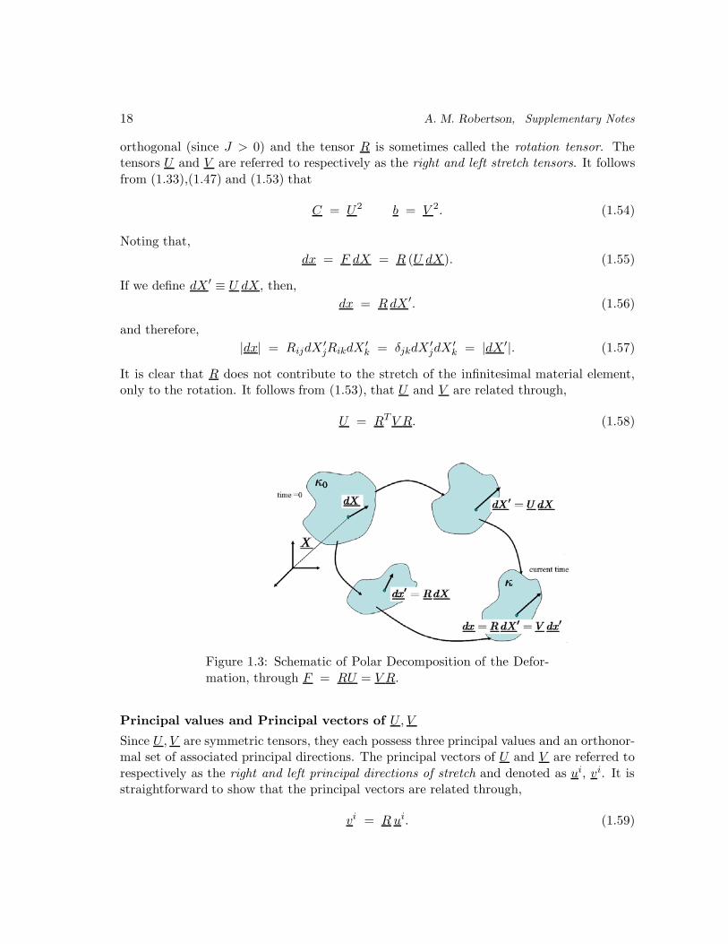
orthogonal (since J > 0) and the tensor R is sometimes called the rotation tensor. Thetensors U and V are referred to respectively as the right and left stretch tensors. It followsfrom (1.33),(1.47) and (1.53) that

C = U2 b = V 2. (1.54)

Noting that,dx = F dX = R (U dX). (1.55)

If we define dX ′ ≡ U dX, then,dx = RdX ′. (1.56)

and therefore,|dx| = RijdX

′jRikdX

′k = δjkdX

′jdX

′k = |dX ′|. (1.57)

It is clear that R does not contribute to the stretch of the infinitesimal material element,only to the rotation. It follows from (1.53), that U and V are related through,

U = RTV R. (1.58)

Figure 1.3: Schematic of Polar Decomposition of the Defor-mation, through F = RU = V R.

Principal values and Principal vectors of U, V

Since U, V are symmetric tensors, they each possess three principal values and an orthonor-mal set of associated principal directions. The principal vectors of U and V are referred torespectively as the right and left principal directions of stretch and denoted as ui, vi. It isstraightforward to show that the principal vectors are related through,

vi = Rui. (1.59)


and the principal values of U and V are identical. Therefore, U and V can be representedas (sum on i),

U = λiui ⊗ ui V = λiv

i ⊗ vi. (1.60)

It then follows that (sum on i),

F = λivi ⊗ ui, R = vi ⊗ ui, C = λ2

iui ⊗ ui, B = λ2

i vi ⊗ vi. (1.61)

1.9 Other Strain Measures

As discussed earlier, the choice of stretch or strain measure is not unique. One alternativeis the Hencky strain 2. �

�

�

�HenckyStrain :

Material Form: ln U

Spatial Form: ln V

(1.62)

Another choice is the Biot strain,�

�

�

�BiotStrain :

Material Form: U − I

Spatial Form: V − I

(1.63)

More generally, we can define,

(Un − I), (V n − I), (1.64)

where n = 2 and n = −2 we recover the Euler-Almansi and the Green-Lagrange strainsdiscussed earlier.

1.10 Velocity Gradient

We denote L as the gradient of the spatial form of the velocity vector, so that the componentsof L with respect to rectangular coordinates are

Lij =∂vi(x, t)∂xj

. (1.65)

Recall that any second order tensor can be decomposed into the sum of a symmetric andskew symmetric second order tensor. We can represent L in this way,

�Lij =12

(∂vi

∂xj+∂vj

∂xi

)+

12

(∂vi

∂xj− ∂vj

∂xi

). (1.66)

2Hencky, H.: Uber die Form des Elastizitatsgesetzes bei ideal elastischen Stoffen. Zeit. Tech. Phys., vol.9, 1928, pp. 215-220, 457


We denote the symmetric part of L by D:

��

��

Rate of Deformation Tensoror

Rate of Strain Tensor

⎫⎬⎭ D =

12(gradL + gradTL

).

and the skew-symmetric part of L by W :

��

��

Spin Tensoror

Vorticity Tensor

⎫⎬⎭ W =

12(gradL − gradTL

).

In indicial notation,

Dij =12

(∂vi

∂xj+∂vj

∂xi

), Wij =

12

(∂vi

∂xj− ∂vj

∂xi

). (1.67)

Physical Significance of Diagonal Elements of D

The physical significance of D can be studied by considering the rate of change in magnitudeof an infinitesimal material element dx of length ds. We first consider the rate of chance ofds2 which is equal to

D(ds2)Dt

= 2 dxiDdxi

Dt. (1.68)

The rate of change in the infinitesimal material element dx is,

Ddxi

Dt=

Ddxi

Dt

=∂FiA

∂tdXA

=∂2χi(X, t)∂t∂ XA

dXA

=∂vi

∂xjFjA dXA

= Lijdxj

(1.69)

and so from (1.68) and (1.69) we find,

D(ds2)Dt

= 2 dx · (Ddx). (1.70)


and thus,Dds

Dt=

dx · (Ddx)ds

. (1.71)

We can interpret the meaning of each of the diagonal elements of D by judicious choice ofdx. For example, choosing dx = dse1 at time t, we find that

Dds

Dt= D11ds. (1.72)

Namely, D11 is the rate of change of ds divided by ds of a material element which at time tis aligned with the e1 axis. So, for a physical flow, if we expect that such a material elementdoes not change length at time t, then D11 = 0. Alternatively, if we expect that it is gettinglonger, then D11 > 0. The other diagonal elements can be interpreted in a similar way.

Physical significance of off-diagonal elements of D

Now consider two infinitesimal material elements x(1) and x(2) which intersect at angle αwith lengths |dx| and |dy| respectively. Then,

cosα =dx(1) · dx(2)

|dx(1)| |dx(2)| (1.73)

and therefore,

D

Dtcosα =

D

Dt

(dx(2) · dx(2)

|dx(1)| |dx(2)|

)

=D

Dt

(dx(1) · dx(2)

) 1|dx(1)| |dx(2)| − dx(1) · dx(1)

|dx(1)|2 |dx(2)|2D

Dt

(|dx(1)| |dx(2)|

)

= 2dx(2) · (Ddx(1))|dx(1)| |dx| − dx(1) · dx(2)

|dx(1)|2 |dx(2)|2D

Dt

(|dx(1)| |dx(2)|

)(1.74)

For example, if are interested in the physical meaning of D12, we can consider (1.74) for twoinfinitesimal material elements, dx(1), dx(2) which at time t are parallel to the base vectorse1 and e2. Since they are orthogonal, the second term in (1.74) drops out and we can show,the rate of change of the angle between these two vectors at time t is

Dα

Dt= − 2D12. (1.75)

Therefore, the value of D12(x, t) is the rate of change of angle between the two infinitesimalvectors which at time t are located at position x and parallel to base vectors, e1 and e2.Similar arguments holds for the other off diagonal elements. Notice that this interpretationof the components of D does not require knowledge of the behavior of specific materialelements. Rather D(x, t) is related to the rate of change of material elements which at timet are located at position x.


1.10.1 Vorticity Vector and Vorticity Tensor

Recall the definition of the vorticity, ω of the velocity vector3,

ω ≡ curlv, or ωi ≡ εijk∂vk

∂xj. (1.76)

It is a nice exercise to show that the components of the vorticity vector are related to thecomponents of the vorticity tensor through,

ωi = − εijk Wjk, and Wij = − 12εijk ωk. (1.77)

1.11 Special Motions

1.11.1 Isochoric Motions

Isochoric motions are those in which the volume occupied by any set of fixed materialparticles is unchanged during the motion. Namely, dv = dV for isochoric motions at allpoints in the body. A material does not have to be incompressible to undergo isochoricmotions. However, all motions experienced by incompressible materials must be isochoric.We see from (1.28) that if a motion is isochoric then the value of J is one throughout themotion. In this case, we have from (1.31) that the divergence of v is equal to zero andhence the trace of D is zero. In summary, each of the following are necessary and sufficientconditions for a motion to be isochoric,�

�

�

�Necessary and sufficient conditions for an isochoric motion

dv = dV, J = 1, DJ/Dt = 0, div v = 0, traceD = 0,at all points in the body, for all times during the motion.

1.11.2 Irrotational Motions

Irrotational motions are those for which the vorticity is zero. From (1.77), the vorticitytensor W is zero for irrotational motions.

1.11.3 Homogeneous Deformations

A motion is said to be a homogeneous deformation if F is independent of the material point.In this case, the can integrate (1.21) with respect to X to obtain,

x = F (t)X + c(t). (1.78)3Note that alternate definitions of vorticity are sometimes used. For example, sometimes the vorticity

is defined as the negative of that given in (1.76). In other cases, the vorticity is taken to be twice that in(1.76).


It then follows directly that, R, U, B, C, E, e and J are constant throughout the body (andare also only functions of time). Hence, in a homogeneous deformation, all material elementswhich are parallel, experience the same change in length and orientation. In particular, astraight material line in the reference configuration will remain straight throughout the de-formation though it may change orientation.

As discussed below, two special categories of homogeneous deformations are Rigid Mo-tions in which (U = I) and Pure Homogeneous Deformations in which (R = I).

1.11.4 Rigid Motions

We shall say that body B performs a rigid motion if and only if the distance between twoarbitrary material points remains the same for all time during the motion. Equivalently wecan say, the for all arbitrary X, Y in B,

|x− y| = |X − Y |, (1.79)

for all times during the motion, where x = χ(X, t) and y = χ(Y , t). It can be shown(homework) that the most general rigid motion can be written as,

x = F (t)X + c(t), with FF T = I. (1.80)

where it should be recalled from (1.3) that the detF > 0. Namely, a rigid body motion isa homogeneous deformation for which F is proper orthogonal. Alternatively, we can write,

x− y = F (t)(X − Y ), with FFT = I. (1.81)

It can be shown (homework), that a necessary and sufficient condition for a motion to berigid is that F = R for all points in B at all times during the rigid motion. Similarly, wecan show,

C = I, b = I, U = I V = I,E = 0, e = 0, ds = dS λ = 1.

(1.82)

In addition, we see from (1.71) that for rigid motions, D must be identically zero at allpoints in the body for all time during the motion. Alternatively, we see from (1.71) thatmotions in which D is zero at all points in the body for all time are rigid motions. Namely,a motion of B is rigid if and only if D is identically zero for all points in B throughout theduration of the motion and therefore, L = W .

Velocity field for a rigid motion

Taking the material derivative of (3.66), we find,

v(x, t) − v(y, t) = ˙F (t)(X − Y ). (1.83)


It then follows directly from (3.66) that (X − Y ) = F T (x− y) so that,

v(x, t) − v(y, t) = F FT (x− y). (1.84)

Then, recalling that in general F = LF and for a rigid motion L = W ,

v(x, t) − v(y, t) = W (x− y). (1.85)

It then follows from (1.77),

v(x, t) − v(y, t) =12ω × (x− y). (1.86)

1.11.5 Pure Homogeneous Deformation

Pure homogeneous deformations are homogeneous deformations with R = I. Namely,F = U(t) = V (t), so

x = U(t)X + c(t). (1.87)

We will consider two special types of Pure Homogeneous Deformations: Plane Strain andAxisymmetric Strain.

1.11.6 Plane Strain

In Plane Strain, the deformation is confined to one plane and U and the eigenvalues of U areof the form (λ, μ, 1). Namely, with respect to a basis composed of the principal directionsof U , the components of the F can be written as,

[F ] = [U ] =

⎡⎣ λ 0 0

0 μ 00 0 1

⎤⎦ (1.88)

or, in shorthand, we will write:

diag(F ) = diag(U) = (λ, μ, 1). (1.89)

It is clear that for the deformation given in (1.96) that material lines elements parallel tou3 direction do not undergo any stretching or rotation, hence the name plane strain. Wewill consider three special cases of plane strain.

Uniaxial strainUniaxial strain is a particular case of plane strain with

diag(F ) = diag(U) = (λ, 1, 1). (1.90)


Axisymmetric Plane Strain

An important special case of plane strain is axisymmetric plane strain in which

diag(F ) = diag(U) = (λ, λ, 1). (1.91)

Isochoric Plane Strain (or “Pure Shear”)

Isochoric plane strain is a special case of plane strain in which the determinant of thedeformation gradient tensor must be one, and so,

diag(F ) = diag(U) = (λ, 1/λ, 1). (1.92)

1.11.7 Axisymmetric Strain

Axisymmetric strain is a pure homogeneous deformation for which there exists an orthonor-mal basis such that,

diag(F ) = diag(U) = (μ, μ, λ). (1.93)

Two types of plane strain considered above, are also types of axisymmetric strain: uniaxialstrain and axisymmetric plane strain. We will consider two additional types of axisymmetricstrain: pure dilation and isochoric axisymmetric strain.

Pure Dilation

A pure dilation is a special pure axisymmetric homogeneous deformation for which

U = λI (1.94)

where λ are the principal stretches of U . It follows from, (1.32) that,

dx = λ dXo, and ds2 = λ2 dS2 (1.95)

for all infinitesimal vectors dX. Notice that infinitesimal elements do not change direction,during the deformation, they only undergo stretch. In addition, every material elementundergoes the same stretch. As a result, a spherical volume will remain spherical andmore generally, bodies will remain geometrically similar with a change of scale λ. The onlyisochoric pure dilation is one for which λ = 1.

Isochoric Axisymmetric Strain

In isochoric axisymmetric strain, the determinant of the deformation tensor must be iden-tically one and hence,

diag(F ) = diag(U) = (1/√λ, 1/

√λ, λ). (1.96)


Homogeneous Deformations: ∇F = 0Rigid Motions F = R

Pure Homogeneous Deformations diag(F ) = diag(U) = (λ, μ, γ)

Plane Strain diag(U) = (λ, μ, 1)

Uniaxial Strain diag(U) = (λ, 1, 1)

Axisymmetric Plane Strain diag(U) = (λ, λ, 1)

Isochoric Plane Strain (”Pure Shear”) diag(U) = (1/λ, λ, 1)

Axisymmetric Strain diag(U) = (μ, μ, λ)

Uniaxial Strain diag(U) = (1, 1, λ)

Axisymmetric Plane Strain diag(U) = (μ, μ, 1)

Pure Dilation diag(U) = (λ, λ, λ)

Isochoric Axisymmetric Strain diag(U) = (1/√λ, 1/

√λ, λ)

with a discussion of one-parameter deformations.

Other Homogeneous Deformations

Notice that there are an infinite number of deformations which, under a polar decomposition,have the same U as these pure homogeneous deformations, but for which R, though constantis not equal to the identity tensor. Once simple way to check this is to compare the principalinvariants of C. Consider the case of simple shear.Simple ShearIn simple shear, the deformation can be described relative to Cartesian coordinates through,

x = X + κ(t)X2e1. (1.97)

A rectangular block with sides parallel to the coordinate axes is transformed in simple shearto a skewed parallel piped. Material planes parallel to the X-axis remain parallel to theaxis, though shifted by κ(t)X2 in the X1-direction (the direction of shear). These materialplanes are called glide planes and κ(t) is called the amount of shear. Material planes parallelto the X2-axis are rotated through an angle γ, the angle of shear, where tanγ = K. TheX1−X2 plane is called the plane of shear. The components of the corresponding deformationgradient tensor,

[F ] =

⎡⎢⎢⎢⎢⎣

1 κ(t) 0

0 1 0

0 0 1

⎤⎥⎥⎥⎥⎦ , (1.98)


and the components of the left and right Cauchy-Green strain tensors are

[B] =

⎡⎢⎢⎢⎢⎣

1 + κ(t)2 κ(t) 0

κ(t) 1 0

0 0 1

⎤⎥⎥⎥⎥⎦ , [C] =

⎡⎢⎢⎢⎢⎣

1 κ(t) 0

κ(t) 1 + κ(t)2 0

0 0 1

⎤⎥⎥⎥⎥⎦ . (1.99)

As can be seen in (1.99), simple shear is a homogeneous, planar isochoric deformation.Noting, that in a homogeneous plane deformation, without loss in generality the rotationtensor can be represnted as,

[R] =

⎡⎢⎢⎢⎢⎣

cosω − sinω 0

sinω cosω 0

0 0 1

⎤⎥⎥⎥⎥⎦ . (1.100)

It then follows from (1.99) and (1.100) that,

[U = RTF

]=

⎡⎢⎢⎢⎢⎣

cosω κ(t) cosω + sinω 0

− sinω −κ(t) sinω + cosω 0

0 0 1

⎤⎥⎥⎥⎥⎦ . (1.101)

Due to the symmetry of U , U12 = U21 and hence we can conclude from (1.101), thattanω = −1/2κ(t). It then follows that

[R] =1√

4 + K2(t)

⎡⎢⎢⎢⎢⎢⎣

2 κ(t) 0

−κ(t) 2 0

0 0√

4 +K2(t)

⎤⎥⎥⎥⎥⎥⎦ , (1.102)

[U ] =1√

4 +K2(t)

⎡⎢⎢⎢⎢⎢⎣

2 κ(t) 0

κ(t) 2 + κ(t)2 0

0 0√

4 +K2(t)

⎤⎥⎥⎥⎥⎥⎦ . (1.103)

The principal values and principal directions of U are,

(λ1, λ2, λ3) = (λ,1λ, 1), where λ ≡ 1

2(K +

√4 +K2), (1.104)


and

u1 =1√

1 + λ2(e1 + λ e2), u2 =

1√1 + λ2

(−λ e1 + e2), u3 = e3. (1.105)

It follows that an infinitesimal line element which parallel to the u1 in the reference config-uration, will increase in length by λ while and infinitesimal line element which is parallel tou2 in the reference configuration, will decrease in length by 1/λ.

1.11.8 Non-Homogeneous Deformations

Shearing DeformationsRecall, that in the section on homogeneous deformations, we considered isochoric planestrain (pure shear) and simple shear. For both these deformations, the principal invariantsof C were of the form,

I = II and III = 1, (1.106)

and for simple shear I = 3 + κ2. We can generalize this to define shearing deformations(either homogeneous or non-homogeneous) as any deformations for which the principalinvariants are of the from (1.106) where, in general, I may depend on the position in thebody and time. As in simple shear, we define the amount of shear, κ, through κ2 = I−3. Itfollows that all isochoric plane strains, either homogeneous or non-homogeneous are shearingdeformations.

Exercise 1.11.1 Prove the relationships between the components of the vorticity tensor and vorticity

vector given in (1.77).

Exercise 1.11.2 Use the transport theorem to provide an alternative proof that for an isochoric motion,

the divergence of the velocity vector is zero.

Chapter 2

Governing Equations

2.1 Governing Equations

Before discussing the governing equations, it is helpful to review the transport theorem.

The Transport Theorem

The transport theorem for an arbitrary scalar function φ of position x and time t is�

�

d

dt

∫Vφ(x, t) dv =

∫V

(Dφ

Dt+ φ divv

)dv (2.1)

where v is the velocity vector and V(t) be an arbitrary material volume of the body in thepresent configuration at time t.ProofRecall that the integral of a function φ(x, t) over the an arbitrary material volume of thebody in the present configuration at time t can be written with respect to an integral overthe corresponding material volume V0 in the reference configuration κ0∫

V(t)

φ(x, t)dv =∫V0

φ(X, t)JdV, (2.2)

where dv = JdV . Taking the time derivative of (2.2), we find

d

dt

∫Vφ(x, t) dv =

d

dt

∫Vo

(φ(X, t) J

)dV

=∫Vo

(Dφ

DtJ + φ

DJ

Dt

)dV

=∫Vo

(Dφ

Dt+ φdivv

)JdV

(2.3)

29


where we have made use of (1.31) and the fact that Vo is independent of time. Eq. (2.1)follows directly from this result. Alternatively, it is sometimes convenient to write (2.3) as,

d

dt

∫V(t)

φ(x, t)dv =∫V(t)

∂φ(x, t)∂t

dv +∫

δV(t)φ(x, t)v(x, t) · ndv (2.4)

where V(t) is bounded by a closed regular surface δV with outward normal n(x, t). In whatfollows, we will also make use of the following theorem:Theorem:�

�

�

�

If φ(x, t)is continuous in the region R(t), then a necessary and sufficientcondition for∫

V(t)φ(x, t)dv = 0 for every V(t) ⊆ R(t)

is

φ(x, t) = 0 all x in R.

(2.5)

2.1.1 Conservation of Mass

The mass M of a section V(t) of the body at time t is

M =∫V(t)

ρ(x, t) dv, (2.6)

where ρ is the mass density of the body at time t. The mass M0 of the same materialpoints in configuration κ0 is,

M0 =∫V0

ρ0(X) dV, (2.7)

where ρ0(X) is the mass density of the material in κ0. The principle of conservation of massis the postulate that the mass of the body in an arbitrary material volume V(t), does notchange in time

M(t) = M0 for all time t. (2.8)

Transforming the volume integral in (2.6) over V(t) to an integral over V0, using this resultwith (2.7) and (2.8), and making necessary continuity assumptions, we have directly that

ρ J = ρ0 all X ⊆ R0. (2.9)

This is the local Lagrangian form of conservation of mass. Alternatively, taking the timederivative of (2.8) and using (2.6) and (2.6), it follows that

d

dt

∫V(t)

ρ(x, t) dv = 0. (2.10)


Making use of the Transport Theorem, we can write the principle of conservation of mass(2.10) as,

0 =∫V(t)

(Dρ

Dt+ ρ(x, t)div v(x, t)

)dv. (2.11)

Making suitable assumptions about continuity of the field variables and using (??), weobtain the local form of (2.11),

Dρ

Dt+ ρ divv = 0 allx ⊆ R (2.12)

or in indicial notation,Dρ

Dt+ ρ

∂vi

∂xi= 0 all x ⊆ R. (2.13)

Implications of Conservation of Mass for Incompressible Materials

The motion of an incompressible materials is constrained to be isochoric, in which case forall motions: the divergence of the velocity vector is constrained to be zero and J is one. Inthis case, the local form of the conservation of mass in Eulerian form, (2.31), reduces to,

Dρ

Dt= 0 all x ⊆ R. (2.14)

and (2.9) becomesρ = ρ0 all X ⊆ R0. (2.15)

Note that the even though the material derivative of the density it is zero, it is notnecessary that the density be constant in space. For example, a stratified fluid with densitydistribution, ρ = ρ0 + αy, where α is a constant, can experience simple shear. Simple shearrefers to the velocity field, v = γ yex. This flow field has particular importance becauseit the solution for steady, fully developed flow between two parallel plates driven by themotion of the upper plate v = Uex. The lower plate is located in the plane y = 0 and theupper plate in the plane y = h. If the plates are separated by a distance h then γ = U/h.It is easily seen that this motion is isochoric, a necessary condition for an incompressiblefluid to experience this motion. In addition,

Dρ

Dt=∂ρ

∂t+

∂ρ

∂xivi = 0 (2.16)

for the stratified fluid and given motion and therefore conservation of mass is satisfied. Aswill be discussed at a later point, this motion is compatable with the balance of linearmomentum for both inviscid and linearly viscous fluids. In fact, a much wider class of fluidscan be shown to undergo this motion.


2.1.2 Balance of Linear Momentum

The postulate of balance of linear momentum is the statement that the rate of change oflinear momentum of a fixed mass of the body is equal to the sum of the forces acting onthe body. These forces can show up as body forces, or as forces due to stress vectors actingon the surface of the body,

d

dt

∫V(t)

ρv dv =∫V(t)

ρ bdv +∫

δV(t)t da (2.17)

where b is the body force per unit mass, t(x, t, n) is the surface force acting on the body inthe current configuration per unit area of δV and n is the unit normal to the surface δV atx at time t. Note that stress vector depends on position, time and the unit normal to thesurface at x. The first and second integrals on the right hand side of (2.17) represent thecontributions due to body forces and to surface forces respectively.

It is somewhat problematic that the stress vector depends on the surface under con-sideration. Fortunately, we can show that it is possible (under certain conditions) to showthat this dependence is linear. Fortunately, as discussed below, the existence of a secondorder tensor, T can be shown, where,

t = t(x, t, n) = T (x, t)n. (2.18)

and T is called the Cauchy stress tensor.

Cauchy’s Lemma

Consider an arbitarry part of the material region of the body B which occupies a part V inthe present configuration at time t with bounding surface ∂V . Let V be divided into tworegions V1, V2 separated by a surface σ. Further, let ∂V1, ∂V2 refer to the boundaries ofV1, V2, respectively and let ∂V ′, ∂V ′′ be the portions of the boundaries of V1, V2 such that

∂V ′ = ∂V1 ∩ ∂V , ∂V ′′ = ∂V2 ∩ ∂V . (2.19)

Thus,

V = V1 ∪ V2, ∂V = ∂V ′ ∪ ∂V ′′ ∂V1 = ∂V ′ ∪ σ, ∂V2 = ∂V ′′ ∪ σ. (2.20)

Now recall the balance of linear momentum for the arbitrary material region V ,

d

dt

∫Pρv dv =

∫Vρ bdv +

∫∂Vt da. (2.21)

The balance of linear momentum can also be considered separately for parts V1 and V2,

d

dt

∫V1

ρv dv =∫V1

ρ bdv +∫

∂V1

t da,

d

dt

∫V2

ρv dv =∫V2

ρ bdv +∫

∂V2

t da.

(2.22)


as well as the union of these regions V1 ∪ V2, be

d

dt

∫V1∪V2

ρv dv =∫V1∪V2

ρ bdv +∫

∂V1∪∂V2

t da. (2.23)

The stress vector t(x, t; n) is (2.22)1 acting over the boundary ∂V1 results from contactforces exerted by the material on one side of the boundary (exterior to ∂V1) on the materialon the other side. Similar results hold for the stress vectors in (2.22)2 and (2.23). It shouldbe emphasized that the stress vector in (2.22)1 over ∂V ′ ∪ σ represents the contact forceexerted in V1 across the surface. The approriate normals associated with t(x, t; n) on σ areequal in magnitude and opposite in sign. In particular, if n is the outward normal at x onsurface σ of V1, then the outward normal at x on surface σ of V2 is −n.

After combining (2.22)1 and (2.22)2 and subtracting (2.23), we obtain,∫σ

[t(x, t; n) − t(x, t;−n)] da = 0. (2.24)

Assuming that the stress vector is a continuous function of position and n, it follows that�

�

�

�

Cauchy’s Lemma

t(x, t; n) = − t(x, t;−n).

The stress vectors acting on opposite sides of the same surface at a givenpoint and time are equal in magnitude and opposite in sign.

(2.25)

Existence of the stress tensor and its relationship to the stress vector

At this point, it has not been shown in what way the stress vector depend on the normalto the surface. It can be shown that there exists a second order tensor T (x, t) such that�

�

�

�t(x, t; n) = T (x, t) · n or tk(x, t; n) = Tki(x, t) ni

The stress vector depends linearly on the normal to the surface.(2.26)

The second order T is called the Cauchy stress tensor. Significantly, T is independent ofthe surface n. Sometimes, it is convenient to write this result in matrix form,⎡

⎣ t1t2t3

⎤⎦ =

⎡⎣ T11 T12 T13

T21 T22 T23

T31 T32 T33

⎤⎦⎡⎣ n1

n2

n3

⎤⎦ . (2.27)

So, for example, if we consider a surface with normal n = e1, then⎡⎣ n1

n2

n3

⎤⎦ =

⎡⎣ 1

00

⎤⎦ and therefore

⎡⎣ t1t2t3

⎤⎦ =

⎡⎣ T11

T21

T31

⎤⎦ , (2.28)


or, equivalently,t = T11e1 + T21e2 + T31e3. (2.29)

Making use of the divergence theorem as well as the relationship between the stresstensor and the stress vector, (2.17) can be written as,

d

dt

∫V(t)

ρv dv =∫V(t)

(ρb + divT ) dv. (2.30)

The local form of the equation of linear momentum can be obtained from (2.30) by usingthe Transport Theorem and making suitable assumptions about the continuity of the fieldvariables,

ρa = ρb + divT all x ⊆ R (2.31)

or, using index notation,

ρai = ρbi +∂Tij

∂xjall x ⊆ R, (2.32)

where the acceleration is given in (1.13) and (1.18). It is often convenient to represent T asthe sum of a deviatoric and spherical part.

T = τ + t I, (2.33)

where,

τii = 0, and t =13Tkk. (2.34)

The tensor τ is often referred to as the deviatoric part of T and tI as the spherical part.When the Cauchy stress tensor is decomposed in this way, −t is often called the pressureand denoted by p. Using the decomposition, (2.33), the balance of linear momentum canbe written as,

ρa = −∇p + div τ + ρb all x ⊆ R. (2.35)

Alternatively,

ρai = − ∂p

∂xi+

∂τij∂xj

+ ρbi all x ⊆ R. (2.36)

For compressible fluids, p is the thermodynamic pressure and an equation of state is required,for example the ideal gas law. For incompressible fluids, p is a mechanical pressure arisingfrom the constraint of incompressibility. No equation of state is necessary, rather, p will bedetermined as part of the solution to the governing equations and boundary conditions.

Piola-Kirchhoff Stress TensorWe now consider p, the surface force acting on the body in the current configuration perunit area of δV0. The vectors p and t are related through,∫

δV0

p dA =∫

δVt da. (2.37)


The balance of linear momentum can also be written with respect to δV0 and V0 throughthe use of dv = JdV and ρJ = ρ0 as∫

V0

ρ0a dV =∫V0

ρ0 b dV0 +∫

δV0

p dA. (2.38)

Similar to the discussion for t, it can be shown that

p(X, t, N) = −p(X, t, N) (2.39)

andp(X, t, N) = P (X, t)N, (2.40)

where P is the first Piola-Kirchoff stress tensor and N is the unit normal to the surface δVat X. It then follows from (2.40) and the relationship between da = JF−T dA, that,

P = J T F−T all X ⊆ R0. (2.41)

The first Piolo-Kirchoff tensor is not symmetric. It is often convenient for numerical pur-poses to define a symmetric stress tensor S, called the second Piola-Kirchoff stress, relatedto P and T through

S = F−1P , and S = J F−1TF−T . (2.42)

Making use of (2.40) in , it follows from (2.38) that,∫V0

ρ0a dV =∫V0

(ρ0 b + DivP ) dV. (2.43)

The corresponding local form of (2.43) is,

ρ0a = ρ0 b + DivP all X ⊆ R0. (2.44)

2.1.3 Balance of Angular Momentum

The balance of angular momentum is the statement that the rate of change of moment ofmomentum of a material volume is equal to the sum of the all the moments acting on thepart of the body. The integral form of the balance of angular momentum, is in the absenceof body couples,

d

dt

∫V(t)

ρx× v dv =∫V(t)

ρ x× b dv +∫dV(t)

x× t da. (2.45)


In writing (2.45), we have assumed there are no body couples c per unit volume acting onthe body which would contribute an additional torque,∫

V(t)ρ cdv. (2.46)

Making use of the balance of linear momentum, it can be shown that (2.45) reduces to therequirement that the Cauchy stress tensor must be symmetric,

T = T T all x ⊆ R. (2.47)

The balance of angular momentum can also be written with respect to δV0 and V0 throughthe use of dv = JdV and ρJ = ρ0 as∫

P0

ρ0x× adV =∫P0

ρ0 x× b dV +∫

δPx× p dA, (2.48)

The corresponding local form is,

PFT = FP T all X ⊆ R0 (2.49)

Notice that p is not in general symmetric. The second Piola-Kirchhoff stress tensor, S isdefined through,

S = F−1P or SAB = F−1Ai PiB (2.50)

all X0 ⊆ R0 and hence it follows from (2.48) that S is symmetric. Additionally, this means,

S = JF−1TF−T or SAB = JF−1iA TijF

−1Bj . (2.51)

2.1.4 Mechanical Energy Equation

It is sometimes useful to consider the Mechanical Energy Equation which is obtained fromthe equation of linear momentum making use of the equation of conservation of mass. Ifwe take the inner product of the velocity vector and the local form of the equation of linearmomentum (2.32) we obtain,

12ρD

Dt(vivi) =

∂Tij

∂xjvi + ρbivi all x ⊆ R. (2.52)

An integral form of this equation can be obtained by integrating (2.52) over a fixed regionof the body (same material particles) occupying region V(t) with surface ∂V(t), to obtain,

d

dt

∫V(t)

12ρv · vdv =

∫δV(t)

t · vda −∫V(t)

T : Ddv +∫V(t)

ρb · vdv. (2.53)


where we have made use of the divergence theorem and the conservation of mass. For futurereferece, we introduce the following notation for terms in (2.55):

K ≡∫V(t)

12ρv · vdv = kinetic energy in V(t)

Rc ≡∫

δV(t)t · vda = rate of work done by surface forces on the boundary δV(t)

Rb ≡∫V(t)

ρb · vdv = rate of work done on the material volume V(t) by body forces

Pint ≡∫V(t)

T : Ddv = rate of internal work in the material volume V(t).

(2.54)The scalar, T : D is the rate of work by stresses per unit volume of the body and is oftencalled the stress power. The sum of Rc and Rb is then the rate of work by external forceson the material volume.In summary, we can write the mechanical energy equation as�

��

Mechanical Energy Equationd

dtK + Pint = Rc + Rb.

(2.55)

Alternatively, we can start with the local form of linear momentum in Lagrangian form, takethe inner product with the velocity and integrate over the corresponding material regionV0 in κ0. After using the divergence theorem, we can show that we obtain the same form(2.55) with

K =∫V0

12ρ0v · vdV, Rc =

∫δV0

p · vdA, Rb =∫V0

ρ0b · vdV, Pint =∫V0

P : F dV. (2.56)

In fact, this last quantity can also be written with respect to T , P , or S,

Pint =∫V(t)

T : Ddv =∫V0

P : F dV =∫V0

S : EdV. (2.57)

2.1.5 Balance of Energy

If we consider a part of the body V(t) in the current configuration, we can hypothesize theexistence of a scalar called the specific internal energy, u = u(x, t) (internal energy perunit mass). The internal energy for the part V(t) of the body, will then be∫

V(t)

ρudv. (2.58)


We do not go delve into a discussion of entropy here, but remind the reader that the specificinternal energy is related to the Helmholtz potential ψ and the entropy η through,

u = ψ + ηT (2.59)

where T is the absolute temperature. Recall that the kinetic energy of the part V(t)of thebody is ∫

V(t)

12ρv · vdv. (2.60)

Heat may enter the body through the surface dV(t) of the body with outward unit normaln. It can be shown, that this heat flux can be represented as the scalar product of a vectorq and the normal to the surface n. Where q · n positive is associated with heat leaving thesurface and q · n negative is associated with heat entering the surface. In addition, heatmay enter the body as a specific heat supply, r = r(x, t): the heat entering the body perunit mass per unit time. Therefore the rate of heat entering the part V(t) of the body is

−∫dV(t)

q · nda +∫V(t)

ρrdv. (2.61)

The balance of energy is a statement that the rate of increase in internal energy and kineticenergy in the part V(t) of the body is equal to the rate of work by body forces and contactforces plus energies due to heat entering the body per unit time. We can write this statementas

d

dt

∫V(t)

ρ(u+12v · v)dv =

∫dV(t)

t · vda +∫V(t)

ρb · vdv −∫dV(t)

q · nda +∫V(t)

ρrdv (2.62)

where the first integral on the left hand side is the rate of work by contact forces, the secondintegral is the rate of work by body forces. Making suitable assumptions about continuityof the field variables, we can obtain the local form of (2.62),

ρ

(Du

Dt+ v · Dv

Dt

)= T : D + v · (divT ) + ρv · b− divq + ρr. (2.63)

Using results from the mechanical energy equation, we can rewrite (2.63) as�

�

�

�

Local, Eulerian form of Balance of Energy

ρDu

Dt= T : D − divq + ρr,

or

ρDu

Dt= TijDji − ∂qi

∂xi+ ρr.

(2.64)


Similarly, we can write the Lagrangian form of the balance of energy,�

�

�

�

Local, Lagrangian form of Balance of Energy

ρ0u = P T : F − Divq0

+ ρ0r,

or

ρ0u = PiAFiA − ∂q0A

∂XA+ ρ0r.

(2.65)

where ∫V(t)

q · da =∫V0

q0· dA. (2.66)

2.1.6 Clausius-Duhem Inequality

The second law of thermodynamics is formulated in a variety of ways. The Eulerian formof the Clausius-Duhem inequality is,�

�

!

Eulerian form of the Clausius Duhem Inequality

Finite Volume Formd

dt

∫V(t)

ρηdv ≥∫V(t)

ρr

Tdv −

∫V(t)

q · nT

da

(2.67)

The local form is,

η − r

T+

1ρ

div(q

T) ≥ 0. (2.68)

For cases where we use the temperature as an independent variable, it is convenient to makeuse of ψ = u− Tη, in which case, we can write this last result as,

−ρ(ψ + ηT

)+ T : D − 1

Tq · gradT ≥ 0. (2.69)

The Lagrangian form of (2.67) is,�

�

!

Lagrangian form of the Clausius Duhem Inequality

Finite Volume Formd

dt

∫V0

ρ0ηdV ≥∫V0

ρ0r

TdV −

∫V0

q ·NT

dA

(2.70)

η − r

T+

1ρ0

div(q0

T) ≥ 0. (2.71)

and the corresponding local form is,

−ρ0

(ψ + ηT

)+ PT : F − 1

Tq0· GradT ≥ 0. (2.72)


It follows directly from (2.69) and (2.72) that for isothermal processes with no heat transfer(T = constant and q = q

0= 0), the Clausius Duhem Inequality reduces to,�

�

�

�

Isothermal form of the Clausius Duhem Inequality

Eulerian

−ρ ψ + T : D ≥ 0,

Lagrangian

−ρ0 ψ + P T : F ≥ 0.

(2.73)

2.1.7 Summary of Governing Equations:

1 Integral Form for Finite Region V(t) with surface δV, Fixed Material Particleswhere V(t) is an arbitrary material volume such that V(t) ⊆ R(t).

d

dt

∫V(t)

ρ dv = 0.

d

dt

∫V(t)

ρv dv =∫V(t)

ρ bdv +∫

δV(t)t da

d

dt

∫V(t)

ρx× v dv =∫V(t)

ρ x× b dv +∫

δV(t)x× t da.

(2.74)

Corresponding Local Form

Dρ

Dt+ ρdiv v = 0

ρa = ρb + divT

T = T T

ρDu

Dt= T : D − divq + ρr

−ρ(ψ + ηT

)+ T : D − 1

Tq · gradT ≥ 0.

⎫⎪⎪⎪⎪⎪⎪⎪⎪⎪⎪⎪⎪⎬⎪⎪⎪⎪⎪⎪⎪⎪⎪⎪⎪⎪⎭

all x ⊆ R (2.75)

Integral Form for Finite Region V0 with surface δV0, Fixed Material Particles.where V0 is an arbitrary material volume such that V0 ⊆ R0. Note, these equations arefor the current time, but the integrals are written for areas and volumes in the referenceconfiguration. The density used in these equations, ρ0, is the density of the body when it

1This section will be updated with energy equation and clausius duhem inequality


is in the reference configuration. The stress vector p is the surface force acting on the bodyin the current configuration per unit area of δV0.∫

V0

ρ0(X) dV =∫V(t)

ρ(x, t) dv

∫Vρ0a dV =

∫Vρ0 b dV +

∫δVp dA

∫Vρ0x× a dV =

∫Vρ0 x × b dV +

∫δVx × p dA

(2.76)

Corresponding Local Form

ρ J = ρ0

ρ0a = ρ0 b + DivP

PF T = FPT

⎫⎪⎪⎬⎪⎪⎭ all X ⊆ R0 (2.77)

Integral Form for Fixed Finite Region CV with surface CS

d

dt

∫CV

ρ dv +d

dt

∫CS

ρ v · n da = 0

d

dt

∫CVρ vdv +

∫CVρ v v · ndv =

∫CVρ bdv +

∫CS

t da

d

dt

∫CVρ x× v dv +

∫CVρ x× v v · ndv =

∫CV

ρ x× b dv +∫

CSx× t da

(2.78)

2

2.2 Constraints

2.2.1 Incompressible materials - constraint of incompressibility

Suppose a material is constrained to only undergo isochoric motions, so that J = 1 at allpoints in the body for all times during any motion. We call such a material incompressible.If we take the material derivative of the equation J = 1, we find

0 =DJ

Dt= Jdivv = JDii. (2.79)

For such a material, we will assume the stress tensor has two contributions, a part N whichdoes no work for motions of the form (2.79), and an extra stress TE which requires aconstitutive equation,

T = TE + N. (2.80)2Insert section here about state of stress


Namely, we require

N : D = 0, for all symmetric tensors D satisfying D : I = 0. (2.81)

Since A : B = trAB defines an inner product in the six-dimensional space of symmetrictensors, we can restate (2.81) as a geometric requirement that N be orthogonal to all Dwhich are orthogonal to I. Necessarily, N is of the form,

N = −pI (2.82)

where p is an undetermined Lagrange multiplier (scalar). Therefore, the Cauchy stress foran incompressible material will be defined through a constitutive equation of the form,

T = TE − pI. (2.83)

2.2.2 Inextensible Fibers - constraint of inextensibility

Suppose we have a material in which infinitesimal material elements that are parallel toa0 in reference configuration κ0 are constrained to be inextensible during the deformation.For a general motion, an infinitesimal material element dXa0 in κ0 will be mapped todxa = dXF a0 in κ(t) where a0 and a are chosen to have unit length. For this constrainedmotion, dx/dX = 1, so that a = Fa0. It therefore follows that a0 · Ca0 = 1 for the entiredeformation.

If we take the material derivative of this expression, it follows that, for such inextensiblematerials,

0 =D

Dt(a0 ·Ca0)

= a0A(LijFjAFiB + FiALijFjB)a0B

= 2Dij FjA a0A FiB a0B

= 2Dij ajai

= 2D : (a⊗ a)

(2.84)

We assume, a material with inextensible fibers in the a0 direction in κ0, has two contribu-tions to the stress tensor, N , that does no work in motions satisfying the inextensibilityconstraint and an extra stress TE which will be defined through a constitutive equation. Inthis case,

N : D = 0, for all symmetric tensors D satisfying D : (a⊗ a) = 0. (2.85)

Since A : B = trAB defines an inner product in the six-dimensional space of symmetrictensors, we can restate (2.84) as a geometric requirement that N be orthogonal to all Dwhich are orthogonal to a⊗ a. Necessarily, N can be written as,

N = −qa ⊗ a (2.86)

where q is an undetermined Lagrange multiplier (scalar), so that

T = TE − qa⊗ a. (2.87)

Chapter 3

Constitutive Equations

3.1 Restrictions on the Stress Tensor

Thus far, we have discussed governing equations fundamental to any continuum material.To close this system of governing equations, we need to select constitutive models for thematerial of interest. We choose to take a classical approach to this subject, whereby westart with general forms of the constitutive equation and then use fundamental principlesto reduce the class of acceptable constitutive models. Prior to turning attention to theconstitutive theories, we briefly summarize requirements imposed on constitutive modelsin order that they be deemed “physically reasonable”. Here, and in the remainder of thischapter, we focus attention on purely mechanical theories, where, for example, the effect oftemperature variations are negligible. We will disregard any non-mechanical influences andassume the state of the body is determined solely by the kinematical history, (e.g. page56-68 [30]). Motivated by applications to blood flow, in later sections, attention will beconcentrated on incompressible materials.

Principle of coordinate invariance

The constitutive equations must be independent of the coordinate system used to describethe motion of the body.

Principle of determinism for the stress

The stress in a body at the current time is determined by the history of motion of thatbody and independent of any aspect of its future behavior, [19].

Principle of local action

The determination of the stress for a given particle in the body is independent of the motionoutside an arbitrary neighborhood of that particle (see [30], page 57 for a mathematical

43


description of this principle). This principle was originally combined with the previousprinciple [19].

Principle of equipresence

Under this principle, a quantity which appears as an independent variable in one constitutiveequation should be present in all others for that material unless it violates some law ofphysics or rule of invariance (e.g. page 359-360 [30] for an example in the context ofthermoelasticity and historical discussion of this principle).

Principle of material frame indifference

There are two separate principles which embody the concept that the response of the ma-terial should be unaffected by its location and orientation. In the first, the mechanicalresponse of a body is required to be unchanged under a superposed rigid body motion ofthe body if the change in orientation and position of the body is accounted for (e.g. [11] andpages 484-486 of [18]). The second principle is the requirement that the material responseshould be invariant under an arbitrary change of observer. For historical reasons, Truesdelland Noll refer to the first of these principles as the Hooke-Poisson-Cauchy form and thesecond as the Zaremba-Jaumann form. Strictly speaking, these two principles are different,the second being more restrictive since it includes improper orthogonal transformations,such as reflections. Truesdell and Noll provide an interesting discussion of the history ofthese two principles in [30], pages 45-47.

As will be discussed in the remainder of this chapter, invariance requirements play animportant role in continuum mechanics in restricting the form of constitutive equations.

Thermodynamic restrictions

The second law of thermodynamics is the restriction that the total entropy production forall thermodynamic processes is never negative. In the remainder of this chapter, we restrictattention to purely mechanical theories for which thermal effects are negligible. In thiscase, this restriction can be reduced to the statement that the stress power be non-negative[17, 28, 29],

T : D ≥ 0. (3.1)

For example, in the case of an incompressible, Newtonian fluid T = −pI + 2μD and thiscondition can be shown to reduce to the requirement that μ ≥ 0.

Well-posedness

The system of governing equations for the purely mechanical theory arising from the con-servation of mass, balance of linear momentum and the constitutive equation for the stresstensor should be well-posed. By this we mean existence, uniqueness and continuous depen-dence of the solution on the data can be shown (see, e.g. [12]).


Stability of the rest state

One of the methods used to evaluate the range of physically reasonable parameters for amaterial is to evaluate the conditions under which the rest state is stable. It seems physicallyreasonable to exclude ranges of material parameters for which the rest state is unstable toinfinitesimal disturbances. This criterion has been used, for example, for viscoelastic fluids(see, e.g. [4, 15, 8]) as well as fiber fluid mixtures [9].

Attainability

An additional test, which is relatively straightforward and does not require formulationwithin the context of thermodynamics, is to evaluate the attainability of solutions for chosenbenchmark flows for fluids or equilibrium deformations for solids. A constitutive equationwould seem to be physically unreasonable if a chosen steady or time-periodic motion (e.g.steady Couette flow) is unattainable, no matter how gradually the driving mechanism isramped to a constant value and no matter how small this constant value is. Attainabilityof “physically reasonable” steady flows has been studied for Newtonian fluids (e.g. [6, 13, 7]and the literature there cited) and well as for some viscoelastic fluids [22]. We emphasizethat attainability of a given solution should not be confused with an examination of thestability of this solution (e.g. [6]).

Mechanical response of real materials

Experiments on real materials also provide restrictions on the range of material parametersthat are physically reasonable. Since we cannot test every material in existence, strictlyspeaking, we cannot actually “prove” an experimentally based restriction on a constitutiveequation is necessary. Rather, experimental results for certain categories of real materials(e.g. polymeric fluids) provide guidelines for defining a “reasonable” range of parametersfor a given material.

By way of example, in this subsection, we turn attention to some restrictions we mightimpose on a class of fluids called incompressible simple fluids. Briefly, an incompressiblesimple fluid is a material for which the stress at a point and the current time is determined upto a pressure once the strain of each past configuration relative to the present configurationis known (e.g. [3]). Namely, unlike solid materials, we do not need to know the strainrelative to some inherent “natural” configuration. As discussed earlier in this chapter, thedensity of incompressible materials is unchanged during the deformation.

It can be shown that the mechanical behavior of a chosen (but arbitrary) incompressiblesimple fluid is completely determined in some flows, for example simple shear flow, oncethree material functions are known for that fluid. This result is somewhat unexpectedsince an incompressible simple fluid may have many more than three material functions orconstants. By material functions, we mean functions that depend only on the nature ofthe material, not, for example on the experimental conditions. For reasons to be describedbelow, we will refer to these three functions as viscometric functions.


The three viscometric functions can be defined relative to the rectangular componentsof the Cauchy stress tensor Tij given in (1.97) for simple shear,

τ(γ0) = T12 N1(γ0) = T11 − T22 N2(γ0) = T22 − T33. (3.2)

We will refer to the functions τ(γ0),N1(γ0),N2(γ0) as the shear stress function, first normalstress difference and the second normal stress difference, respectively 1. It can be shownthat τ(γ0) is an odd function while N1(γ0) and N2(γ0) are even functions (e.g. pages 70-71of [23]).

Alternatively, we can consider the viscometric functions η, ψ1, ψ2

η(γ0) =T12

γ0ψ1(γ0) =

T11 − T22

γ20

ψ2(γ0) =T22 − T33

γ20

, (3.3)

referred to as the viscosity, first normal stress coefficient and second normal stress coefficient,where γ0 �= 0. For Newtonian fluids, ψ1 and ψ2 are identically zero.

It turns out that simple shear is not the only motion for which the behavior of an incom-pressible simple fluid is completely determined once η, ψ1 and ψ2 are known. While mostflows do not meet this requirement, there are a number of other flows, called viscometricflows, which do (see, e.g. [3]). Viscometric flows include steady, fully developed flow in astraight pipe of constant circular cross section (sometimes called Poiseuille flow) and steady,unidirectional flow between two concentric circular cylinders driven by the rotation of oneor both of the cylinders about their common axis (sometimes called Couette flow). Mostrheometers are designed to generate viscometric flows and can be used to measure one ormore of these material functions.

Based on experimental data for real polymeric fluids, the sign of ψ1 is expected tobe non-negative and the sign of ψ2 to be non-positive [2]. In addition, the ratio of themagnitude of the second normal stress coefficient to the first normal stress coefficient iscommonly believed to be less than one half (e.g. [16, 21]).

Further Comments

Roughly speaking, the five principles given in this subsection restrict the general functionalform of the constitutive equation (e.g. [?] for further details and historical information). Thelatter requirements impose restrictions on the range of parameters for specific constitutivemodels. In the following sections, applications of these restrictions to particular constitutiveequations are considered.

3.1.1 Superposed Rigid Body Motion

Because of its importance in restricting the form of constitutive equations, we now discussin detail the requirement that constitutive equations be invariant to a superposed rigid bodymotion. The fundamental idea is that the constitutive response should be invariant to arigid motion superposed on the original motion.

1There is some variation in the literature for the definitions of normal stress and even the sign of thestress tensor. See page 71 of [23] for a nice discussion of this issue.


Kinematics for a superposed rigid body motion

In this section, we consider two motions of a body: an arbitrary motion

x = χ(X, t) (3.4)

and a second motion which differs from the first by a superposed rigid body motion andpossibly a time shift,

x+ = χ+(X, t+). (3.5)

Namely, the position of a material point which at time t is at position x in the first motion,is at position x+ in the second motion at time t+ = t+ α. Here α is a constant. These aretwo separate motions as seen by the same observer. The spatial description of (3.5) is then,

x+ = χ+(x, t). (3.6)

In a rigid motion the distances between material points in the body are kept constant.Since the second motion differs from the first motion by a rigid body motion, the functionχ+(x, t) must belong to a restricted class of motions.

It can be shown (see appendix), that the most general form for (3.6) is,�

�

�

�

Most General Superposed Rigid Body Motion

x+ = c(t) + Q(t) · x,where Q(t) is a proper orthogonal second order tensor,

(3.7)

orx+

i = c(t)i + Q(t)ij xj. (3.8)

where Q has the properties,

Q ·QT = I, detQ = +1. (3.9)

The vector c can be interpreted as a rigid body translation and Q as a rotation tensor.

Transformation of kinematic quantities under a superposed rigid body motion

We now consider other kinematical quantities under the superposed rigid body motion,(3.7). The velocity vector v, transforms as,

v+ =∂χ+(X, t)

∂t=

dc(t)dt

+dQ

dtx + Qv. (3.10)

We define Ω as

Ω =dQ

dtQT . (3.11)


Recall, that QQT = I , sodQ

dtQT + Q

dQT

dt= 0 (3.12)

and hence, using (3.11) and (3.12), we find,

Ω + ΩT = 0 (3.13)

and therefore, Ω is skew-symmetric. Using the definition of Ω, (3.11), we can write theexpression for v+ as,

v+ =dc(t)dt

+ ΩQx + Qv, (3.14)

andv+i =

dci(t)dt

+ ΩilQlmxm + Qilvl. (3.15)

For future use, we now derive the relationship between L+ and L,

L+ij =

∂v+i

∂x+j

=∂v+

i

∂xk

∂xk

∂x+j

=[ΩilQlmδmk + Qil

∂vl

∂xk

]∂xk

∂x+j

= [ΩilQlk + QilLlk]Qjk

= Ωij + QilLlkQjk

(3.16)

or in coordinate free notation,L+ = Ω + QLQT . (3.17)

Recalling (1.21) and (3.5), it is clear that

F+ =∂χ+(X, t)

∂X, or F+

iA =∂χ+

i (X, t)∂XA

, (3.18)

Using (3.18) and (3.7),

F+iA =

∂χ+i (x, t)∂xj

∂xj

∂XA,

= Qij FjA

(3.19)

and therefore,F+ = QF. (3.20)

Using (3.20) it can also be shown that,

J+ = J. (3.21)


Additionally, the density ρ and the normal to a surface n, transform as,

ρ+ = ρ, n+ = Qn. (3.22)

A scaler, vector or second order tensor which transform as (3.22)1, (3.22)2 and (??)1, re-spectively are called objective.

Exercise 3.1.1 Since the superposed rigid body motions preserve distances between arbitrary pairs of

material points, they must preserve angles between any two vectors. Starting with the form (3.7) show that

this is true.

Exercise 3.1.2 Using F+ = QF , show that

��

��U+ = U, R+ = QR, V + = QV QT

C+ = C, E+ = E, b+ = QbQT , e+ = QeQT ,

Exercise 3.1.3 Using (3.17), it can be shown that

�� D+ = QDQT , W+ = Ω + QWQT .

The stress vector and stress tensor under a superposed rigid body motion

In this section, the relationship between t+ and t and the relationship between T+ and Tare considered. Recall that,

t = t(x, t; n) = T (x, t)n. (3.23)

Therefore,t+ = t+(x+, t; n+) = T+(x+, t)n+. (3.24)

Recall the relationship between the outward unit normal n to a material surface in thecurrent configuration and the corresponding outward unit normal in the superposed motion,n+ = Qn. From this relationship and the linear dependence of the stress vector on n, wemight expect (i) t+ and t to have the same magnitude and (ii) t+ and t to have the sameorientation relative to n+ and n, respectively. Based on these expectations, we introducethe following assumption

t+ = Qt. (3.25)

Using (3.25) and (3.22), it can be shown that,

|t+| = |t|, t+ · n+ = t · n. (3.26)


In addition,

t+ = T+n+ = T+Qn. t+i = T+ij n

+j = = T+

ijQjknk. (3.27)

Using the assumption (3.25) and (3.4),

t+ = Qt = QTn, and t+i = Qijtj = QijTjknk. (3.28)

Combining (3.27) and (3.28), we have that

(T+Q−QT

)n = 0, and

(T+

ijQjk −QijTjk

)nk = 0. (3.29)

Since (3.29) must hold for all n and the expression in brackets is independent of n, we canconclude that the expression in brackets is equal to zero. Hence,

0 = T+Q−QT

= T+QQT −QTQT

= T+ −QTQT

or

⎛⎜⎜⎝

0 = T+ijQjk −QijTjk

= T+ijQjkQlk −QijTjkQlk

= T+il −QijTjkQlk

(3.30)

and therefore,

T+ = QTQT , and T+il = QijTjkQlk. (3.31)

Exercise 3.1.4 Prove the identities in equation (3.26).

3.2 Nonlinear Elastic Material (Cauchy-Elastic Material)

An elastic material in an isothermal theory is characterized by a constitutive equationrelating the stress tensor T to the deformation gradient F , namely

T (X, t) = G(F (X, t), X) (3.32)

where G is a tensor-valued symmetric tensor function called the response function. Notethat Cauchy elastic materials do not depend on the history of the material, but solely on thecurrent state of deformation. For homogeneous bodies, the material behavior is independentof material point. Thus, we would require that the density ρ0 be independent of X andin addition, the manner in which G depends on F be independent of X. Of course, thedeformation need not be homogeneous, in which case, T will indirectly depend on X ,

T = G(F(X, t)). (3.33)


3.2.1 Implications of invariance under a superposed rigid body motion

We will now show, that by requiring Cauchy-elastic materials be invariant under superposedrigid body motions, we restrict the possible forms for G(F (X,t),X). In particular, requiringinvariance under a superposed rigid body motion means the form of the stress response isthe same for the original motion as well as the superposed motion. Therefore, given theform (3.33) for the original motion, then the response for the superposed motion must be,

T+ = G(F+, X) for all proper orthogonal Q. (3.34)

Then using (3.31) with (3.34), we require

QTQT = G(QF,X) for all proper orthogonal Q. (3.35)

orT = QTG(QF,X)Q for all proper orthogonal Q. (3.36)

Without loss in generality, we can choose Q = RT , where F = RU and R is properorthogonal. We then have from (3.36),

T = RG(RRTU,X)RT (3.37)

or��

��

Restrictions on Cauchy-Elasticity tensor due to invariance requirements

T = RG(U,X)RT .

(3.38)We therefore see, that the dependence of T on R is determined a priori whereas the thedependence of T on the stretch tensor U is arbitrary. We shall see that there is a large classof elastic materials for which such a dependence must be of a special form. One example isisotropic materials.

3.3 Viscous fluids

In this section, we consider viscous fluids. Namely, the constitutive response of the materialdepends only on the fluid mass density and the velocity gradient L is of the form T =T (ρ, L). We will now show that if we impose invariance requirements that viscous fluidsmust be isotropic.

Using the relationshipL = W + D (3.39)

we can rewrite the constitutive assumption as

T = T (ρ, D,W ). (3.40)


If the constitutive equation (3.40) is a valid one, then it must hold for all motions, inparticular, it must hold for a superposed rigid motion,

T+ = T (ρ+, D+, W+). (3.41)

Recalling that,T+ = Q · T ·QT , (3.42)

and using (3.41)T (ρ+, D+, W+) = Q · T (ρ, D,W ) ·QT . (3.43)

Recalling,

ρ+ = ρ, D+ = Q ·D ·QT , W+ = Q ·W ·QT + Ω, (3.44)

we can write (3.43) as

T (ρ+, Q ·D ·QT , Q ·W ·QT + Ω) = Q · T (ρ, D,W) ·QT . (3.45)

Now consider a superposed motion, for which at some fixed time t, Q = I , and Ω �= 0. Inthis case, (3.45) becomes,

T (ρ, D,W + Ω) = T (ρ, D,W), (3.46)

for arbitrary choices of the skew-symmetric tensor Ω. It then follows that the responsefunction T cannot depend on W , and so (3.40) is reduced to

T = T (ρ, D), (3.47)

and must satisfyT (ρ, Q ·D ·QT ) = Q · T (ρ, D) ·QT , (3.48)

for all proper orthogonal Q. Then, from (3.48), we can conclude that T (ρ, D) must be asymmetric isotropic tensor function of D, (see, for example, Appendix ??). A representationtheorem for tensors (Appendix ??), states that the most general second order isotropictensor function T (ρ, D) for symmetric second order tensor D, has the form

T = φ0 I + φ1D + φ2D2, (3.49)


where in general φ0, φ1, φ2 are functions of the three principal invariants of D as well as themass density ρ. The three principal invariants of D are,

I = trD = Dii

II =12(tr(D)2 − tr(D ·D)

)=

12

(DiiDjj −DijDji)

III = detD.

(3.50)

3.3.1 Compressible Newtonian Fluid

In the special case of (3.49) for which the dependence of T on D is linear, we recover thecompressible Newtonian fluid. It is typically written as,�

�

�

�Compressible Newtonian Fluid

T = −p I + λ tr(D) I + 2μDwhere p, λ, μ are functions of ρ and λ and μ are viscosity coefficients.

(3.51)

3.3.2 Ideal Fluid

If instead of starting with T = T (ρ, L), we had started with T = T (ρ), we would haveobtained from invariance, that

T (ρ) = Q · T (ρ) ·QT , (3.52)

for all proper orthogonal Q. Therefore, T is an isotropic tensor. Theorem 3 of Appendix Bgives us that the most general form for T is,

��

Ideal Fluid - compressible

T = −p(ρ)I where p is a function of ρ.(3.53)

3.4 Hyperelastic Materials

We have already defined a Cauchy elastic body as one in which the Cauchy stress tensor isa function of the deformation tensor. We now define a hyperelastic material for a purelymechanical theory (in which we do not need to introduce thermodynamic considerationssuch as the balance of energy and Clausius-Duhem inequality). In particular, we will assumethat for hyperelastic materials, the stress power can be represented in the following way

T : D = ρDΣDt

or Tij Dij = ρDΣDt

. (3.54)

where Σ(X, t) is called the strain energy density function or the stored energy perunit mass. In other words, the change in strain energy per unit mass of the body arises


from work done on the body by internal stresses. Note, that such a representation is nottrue for general materials. The total strain energy per unit mass of the body will be denotedby U and is therefore,

U =∫V(t)

ρΣ dv. (3.55)

After integrating (3.54) over an arbitrary volume V(t) and using (2.52) with (3.55), it followsthat,

d

dt(K + U) =

∫∂V(t)

t · vda +∫V(t)

ρb · vdv, (3.56)

where K is the kinetic energy in the body that was defined earlier. We see that forhyperlastic materials, work on the body is directly converted to kinetic or stored energy.Equation (3.56) is the statement that the rate of change of kinetic energy plus the rate ofchange of strain energy equals the rate of work by surface and body forces.

In classical hyperelasticity, it is assumed that the strain energy at each material pointand for all time depends on the deformation gradient at the same point and time,

Σ = Σ(F ,X). (3.57)

For homogeneous materials, the form of the function given in (3.57) will be the same atall points Σ = Σ(F ). A normalization condition is typically applied to the strain energyfunction, so that the strain energy vanishes in the reference configuration where F = I,

Σ(I) = 0. (3.58)

Often a strain energy per unit volume in the reference configuration W is introduced,

U =∫Vo

W dV. (3.59)

and therefore, from (3.55), it follows that, W = ρ J Σ = ρo Σ.

Work done on a hyperelastic material in a closed dynamical process

We now evaluate the work done on a hyperelastic material in a closed dynamic processby the internal stress field. We first consider a dynamical process defined by the pairT andx = χ(X, t) which takes place during the time interval t ∈ [t1, t2]. A dynamicalprocess is closed if F (X, t1) = F (X, t2) for all X ⊆ R0. Now consider the work done ona hyperelastic material as defined by (3.54) at arbitrary material point X during a closeddynamical process,

Work done during t ∈ [t1, t2]∫ t2

t1

T : Ddt =∫ t2

t1

ρ∂Σ(F(X, t))

∂tdt

= ρ (Σ(F (X, t2)) − Σ(F (X, t1)))= 0.

(3.60)


Therefore, the work done by the stress field on a hyperelastic material is zero during a closeddynamical process, independent of the deformation (path) during the interval between t1and t2

3.4.1 Relationship between W and the Helmholtz free energy

If we extend our approach to include the concepts introduced above for thermodynamics,we can relate the strain energy density and strain energy per unit volume to thermodynamicentities, �

�

�

�

Isothermal processes (T = 0)W = ρ0ψ, Σ = ψ

Isentropic processes, (η = 0)W = ρ0u, Σ = u

(3.61)

The details of these results are not shown here, but can be found, for example in [27].

3.4.2 Invariance restrictions

Invariance requirements restrict the form of the functional dependence of the strain energyfunction on F . It follows from the relationship between the strain energy function and thestress tensor, and our invariance requirements on the stress tensor, that

W (F ) = W (QF ), for all proper orthogonal Q. (3.62)

It therefore must hold for Q = R, where F = RU and

W (F ) = W (U). (3.63)

Without loss in generality, the most general form of the strain energy function that satisfiesinvariance can be written as, W = W (C). It is straightforward to show that this is also asufficient condition for the strain energy to satisfy invariance requirements.

Any function of U can also be written as a function of C or E. In particular, it follows


from (3.54) and the chain rule that,�

�

�

�

T =1JF

(∂W

∂C+∂W

∂CT

)FT Tij =

1JFiAFjB

(∂W

∂CAB+

∂W

∂CBA

)

P = F

(∂W

∂C+∂W

∂CT

)or PiB = FiA

(∂W

∂CAB+

∂W

∂CBA

)

S =(∂W

∂C+∂W

∂CT

)SAB =

(∂W

∂CAB+

∂W

∂CBA

)

where W (C) must be a symmetricfunction ofC.

(3.64)We see that the stress field S in a hyperelastic material is completely determined by a scalarfunction of C. In some works, rather than (3.64) the following equations are used,

T = 21JF∂W

∂CF T , P = 2F

∂W

∂C, S = 2

∂W

∂C. (3.65)

As detailed on page 212-213 of [27], care must be taken in using (3.65). Briefly, considerthe example W = c(C2

12 + C221), which can equivalently be written as W = 2cC2

12. If wecalculate S12 and S21 using (3.64), we obtain the same result for both representations of W .However, if we use (3.65), we obtain S12 = S21 = 2(C21 +C21) using the first representaton(correct), but S12 = 8C21, S21 = 0 (incorrect), using the second. It is therefore, in somesense, safer to use (3.64).

3.5 Materials with Symmetry

In this section, we will discuss material symmetry of a body. Some useful references on thissubject are [26, 31], Truesdell and Noll [1992,Section 33] [30] Ogden [1997,Section 4.2.5][20],Spencer [1980, Section 8.2] [25].

Consider an arbitrary material point in the body P , identified by its location in thereference configuration X. In order to discuss the symmetry groups of the body, we needto consider possible changes to the response of a body when the body is rigidly rotated andpossibly translated in the reference configuration. Under this rigid motion, the materialpoint P will moved from X to X∗ by a translation vector c and rotated using an orthogonaltensor A 2,

X∗ = c + A ·X. (3.66)

2A is not necessarily proper orthogonal, meaning we allow reflections


We describe the subsequent motion of the body relative to its position in reference config-uration κ0 or κ∗0 as,

x = χ(X, t) = χ∗(X∗, t). (3.67)

Using the chain rule with (3.66) and (3.67), we obtain a relation between F and F ∗,

FiA =∂χ∗i (X∗, t)∂X∗

B

∂X∗B

∂XA= F ∗

iBABA (3.68)

orF ∗ = F · AT . (3.69)

It therefore follows that,

C∗ = AC AT and b∗ = b. (3.70)

We now consider the change in the response of the body to particular rigid rotations andreflections of the reference configuration, (different choices of A). In particular, we willdescribe symmetries of the body, based on the invariance of their response to rotations inκ0, W (C) = W (C∗). Namely, the symmetry of the body will be stated in terms of the setof A for which

W (C) = W (AC AT ). (3.71)

3.5.1 Isotropic hyperelastic materials

For isotropic materials, (3.71) holds for all orthogonal A and therefore the symmetry groupof an isotropic material includes all rotations about all possible axes and reflections in anyplane. Namely, it is the group of all orthogonal tensors (not just proper), which is the fullorthogonal group in three dimensions 3.�

��

Isotropic Hyperelastic Material

W (C) = W (AC AT )for all orthogonal A(3.72)

From a practical point of view, material isotropy means that if we load a mass of thismaterial which was spherical in the unloaded reference configuration, the response of thematerial will be unaffected by how we rotated or reflected this sphere in κ0.

Note that the mathematical requirement that (3.71) holds for all orthogonal A is a verydifferent requirement than that stated for invariance under a super posed rigid body mo-tion. The invariance requirement must be satisfied for all materials, whereas the condition(3.71) is met by some materials for a particular choice of A and is a material property. Inaddition, we only require that invariance holds for all proper orthogonal tensors, Q, whereasA includes orthogonal tensors which are not proper.

3A material whose symmetry group contains all rotations but no reflections is called Hemitropic. Formany purposes, this distinction is not important


Mathematically, (3.72) implies that W (C) is a scalar valued isotropic tensor functionof C. It then follows from a representation theorem for isotropic scalar functions (see,Appendix D), that without loss in generality, the strain energy function for an isotropic,hyperelastic material may be expressed as a function of the scalar invariants of C, denotedas I1, I2, I3,

W = W (I1, I2, I3), (3.73)

whereI1 = trC = CAA

I2 =12(tr(C)2 − tr(C · C)

)=

12

(CAACBB − CABCAB)

I3 = detC.

(3.74)

Since B and C have the same eigenvalues, their invariants can be shown to be identical.

Stress tensors for an isotropic, elastic material

Using the chain rule with (3.64), (3.73) and results from Appendix D,

∂W

∂CAB=∂W

∂I1

∂I1∂CAB

+∂W

∂I2

∂I2∂CAB

+∂W

∂I3

∂I3∂CAB

=∂W

∂I1δAB +

∂W

∂I2(I1δAB −CAB ) +

∂W

∂I3(I3C−1

AB )(3.75)

Hence,

T =2JF

(∂W

∂I1I +

∂W

∂I2(I1I −C) +

∂W

∂I3(I3C−1

)FT . (3.76)

Recalling that S = JF−1TF−T , were therefore have,�

�

�

�

For an isotropic elastic material

T = 2[I

1/23 W3 I + I

−1/23 (W1 + I1W2) b − I

−1/23 W2 b

2]

and

S = 2[(W1 + I1 W2) I − W2C + W3 I3C

−1]

where Wi ≡ ∂W/∂Ii.

(3.77)

In some cases, it may be of interest to write (3.77) with respect to different powers of thestress tensor. This can easily be done using results from the Cayley-Hamilton Theorem. Inparticular, we can use the result that a second order tensor G satisfies its own characteristicequation so that,

G3 − I1G2 + I2G − I3I = 0, (3.78)


orG2 − I1G + I2I − I3G

−1 = 0. (3.79)

Exercise: It is left as an exercise to use the polar decomposition theorem with A = R(X, t)to shown that if an elastic material with W = W (C) is isotropic, then equivalentlyW = W (b). This last result is also clear from (3.73)

Exercise: Show that W (I∗1 , I∗2 , I

∗3 ) = W (I1, I2, I3) for all orthogonal A, by first showing

that I∗1 = I1, I∗2 = I2, I∗3 = I3 for all orthogonal tensors A, where it should be recalled thatC∗ = ACAT . Namely, show that I1, I2, I3 are invariants of C.

Representative compressible, isotropic strain energy functions

For compressible, isotropic materials, the strain energy may depend on all three invariants.A very general strain energy function for compressible materials is,

W =n∑

i=0

n∑j=0

n∑k=0

cijk(I1 − 3)i (I2 − 3)j (I3 − 3)k (3.80)

where cijk are material constants. There are a number of other well known compressiblestrain energy functions, see, e.g. [27].

Incompressible, isotropic strain energy functions

For incompressible material, I3 is a constant, so the strain energy function will only be afunction of the first two invariants. In addition to the work part of the tensor, there willbe a Lagrange multiplier (denoted as p, but not necessarily equivalent to the mechanicalpressure). Some commonly used isotropic strain energy functions for biological materialsinclude the (i) Mooney-Rivlin, (ii) Neo-Hookean and (iii) exponential strain energy func-tions. The Mooney-Rivlin strain energy function has frequently been used for rubbersand can be written as

W =α

2(I1 − 3) +

β

2(I2 − 3) (3.81)

where α and β are material constants. Notice that W is normalized such that for F = I,W = 0. The neo-Hookean material is a special Mooney-Rivlin material for which β = 0.

A special type of hyperelastic material with an exponential dependence on the firstinvariant of b was introduced by Fung to model the nonlinearly elastic response of biologicaltissue, [?],

W (I1) =α

2γ

(eγ(I1−3) − 1

), (3.82)

where α and γ are material constants. This strain energy has been generalized to include adependence on both I1 and I2

W (I1, I2) = C(eb1(I1−3)+b2(I2−3) − 1

). (3.83)


The components of the Cauchy stress tensor for an isotropic, incompressible hyperelasticmaterial can then be reduced from (3.65) to,

T = −pI + 2 ρ0∂Σ∂I1

b− 2 ρ0∂W

∂I2b−1, (3.84)

where p is the Lagrange multiplier arising from incompressibility. Alternatively, using W =ρ0Σ,

T = −pI + 2∂W

∂I1b− 2

∂W

∂I2b−1. (3.85)

It follows from (3.85) that the corresponding Cauchy stress tensors for these materialsare, for the Mooney-Rivlin material is,�

�

�

�

Neo-Hookean T = −pI + αb

Mooney-Rivlin T = −pI + αb − βb−1

1-term Exponential T = −pI + αeγ(I1−3) b

2-term Exponential T = −pI + 2C(b1 eb1(I1−3) b − b2 eb2(I1−3) b−1)

(3.86)

where it should be recalld that α, β, γ, b1 and b2 are constants.

3.5.2 Transversely Isotropic Materials

A transversely isotropic material has a single axis of symmetry for each material point inthe undeformed configuration. If we select a local Cartesian coordinate system at point P ,we can denote this axis as the Z3 axis. The material is then isotropic in the Z1Z2 plane.This is equivalent to saying the symmetry group contains all rotations about the Z3 axis.With respect to this choice of coordinates, we can therefore write A as

[A] =

⎡⎣ cos θ sin θ 0

− sin θ cos θ 00 0 1

⎤⎦ (3.87)

with θ ∈ [0, 2π]. The strain energy for materials which are transversely isotropic must beinvariant to any rotation in the Z1Z2 plane. Which is equivalent to stating (3.71) holdsfor all A of the form (3.87). For example, a transversely isotropic material might be acomposite material composed of bundle of identical fibers embedded in an isotropic matrixand aligned in the Z3 direction. Based on these symmetry requirements, it can be shownthat, without loss in generality, that a transversely isotropic material can be written as,�

�

�

�

Transversely Isotropic Hyperelastic Material

W = W (I1, I2, I3, I4, I5)

whereI4 = m · Cm and I5 = m · C2m − I2

4 ,

where m is a unit vector parallel to the symmetry axis.

(3.88)


Notice, that I4 is the stretch squared of an infinitesimal element originally aligned with them3 axis. For example, if we choose local coordinate with m = e3, then I4 = C33, whichis the stretch squared of an infinitesimal element originally aligned with e3. Furthermore,I5 = C2

13 + C223. We can obtain some physical insights about I5 by recalling from Section

1.7, that

cosα13 =C13√C11C33

, cosα23 =C23√C22C33

, (3.89)

where α13 is the current angle between two infinitesimal elements which were aligned withthe e1 and e3 axis in κ0. Similarly, α23 is the current angle between two infinitesimalelements which were aligned with the e2 and e3 axis in κ0.

Examples of biological tissue which are sometimes modeled as transversely isotropicinclude skeletal muscle and the layers of heart muscle. For example, each layer is sometimesmodeled as,

W = b1 exp (b2(I1 − 3)) + b3(I4 − 1)m (3.90)

where I4. The variables b1, b2, b3 are material constants and m is an even integer. In thisexample, the first term represents the combined effects of an isotropic matrix and the secondterm represents the fiber contributions.

Orthotropic Materials

A material is orthotropic if for each point of the material in the reference configurationpossesses three mutually orthogonal symmetry planes. The orthogonal axis may vary frompoint to point. An orthotropic material might, for example, be a material composed oforthogonally oriented fibers embedded in an isotropic matrix. Wood is often modeled asorthotropic. Hence, the set of A can be written in component form with respect to the abasis with members parallel to each of these directions,

[A] =

⎡⎣ −1 0 0

0 1 00 0 1

⎤⎦ ,

⎡⎣ 1 0 0

0 −1 00 0 1

⎤⎦ ,

⎡⎣ 0 0 0

0 1 00 0 −1

⎤⎦ . (3.91)

The strain energy function of an orthotropic material must be unaffected by reflections ofeach of the three orthogonal axis. This is equivalent to stating that (3.71) must hold for allA of the form, (3.91). 4

3.6 Finite Elastic Constitutive Equation for Fiber-Reinforced

Material

3.6.1 Constitutive Equation for One Family of Fibers

The previous discussion of anisotropic materials was purely phenomenological. Namely, wedid not directly include information about the constituents of the material. Instead, we

4This section is not complete yet


considered the bulk response. In this section, we will take a different approach in whichthe role of fibers in the material is directly incorporated into the constitutive model. Thisdiscussion will closely follow the work of Spencer, [24, 26]. See also, Sections 6.7 and 6.8 of[14] for a summary of the work of Spencer and further comments. For additional applicationsand background material see [1].

3.6.2 Kinematics

In this section, we consider a body B which occupies a reference configuration κ0 at sometime t = 0. and As the body deforms in time, it will occupy the configuration κ(t) at anarbitrary current time t. This body is assumed to be endowed with fibers in a continuousmanner so that every material point identified by X in κ0 is endowed with a family of fiberswith orientation a0. We assume that during the deformation, fibers will be convected withthe underlying material. In general, the fiber will rotate and stretch. For example, if fiberelement has direction a0 and length ΔX in configuration κ0, it will have a new direction aand new length Δx in the current configuration. For definiteness, we take a0 and a to beunit vectors.

For example, consider a fiber whose ends are at coordinates, X and X + ΔXa0 in κ0

and x and x+ Δxa in κ. Then we can obtain the relationship between a0 and a as follows.From (1.1),

x+ Δxa = χ(X + ΔXa0, t). (3.92)

If we perform a Taylor series expansion of χ(X + ΔXa0) about X ,

x+ Δxa = χ(X, t) + ΔXF (X, t) · a0 + H.O.T.. (3.93)

Taking the limit as ΔX tends to zero, we find,

adx = F (X, t) · a0dX. (3.94)

Therefore, ��

��λa = F (X, t) · a0, λ =

dx

dX. (3.95)

Since a and a0 are unit vectors, it then follows that,

λ2 = a0 · C(X, t) a0. (3.96)

This should not be surprising. We have already shown that diagonal components of Crepresent the stretch squared of an infinitesimal material element which was aligned withthe unit base vectors in the undeformed configuration. We see from (3.96), that the directionof the fiber in κ(t) is determined entirely by C and the fiber direction in κ0.

As before, we consider hyperelastic materials in a purely mechanical setting, by whichwe mean the stress power can be represented as,

T : D = ρDΣDt

or, equivalently T : D = =1J

DW

Dt. (3.97)


Here, we assume the strain energy functions depends on a measure of strain or stretch ofthe bulk material as well as a fiber direction in the reference configuration. Since a flippingof the fiber end to end should not play a role, we assume the dependence on a0 is even, (forexample, through a0 ⊗ a0)5,

W = W (C, a0 ⊗ a0). (3.98)

Note that since a0 is independent of time, the relationship between the strain energy functionand the stress tensor is that same as for the classical hyperelastic material,

T =1JF

(∂W

∂C+

∂W

∂CT

)F T . (3.99)

We will now assume the only anisotropy in the material is due to the fiber orientation ascharacterized by a0. In this case, we will assume that the strain energy is unchanged by anyrigid rotation, translation and possible reflection of both the matrix material and the fibersaround a preferred direction (axis). Mathematically, this is equivalent to the statement

W (C, a0 ⊗ a0) = W (C∗, a∗0 ⊗ a∗0). (3.100)

where,C∗ = A · C ·AT , a∗0 = A · a0 (3.101)

for all orthogonal second order tensorsA. Note that A does not need to be proper orthogonalbecause the response is also invariant to reflections. Substituting the results (3.101) in(3.100), we obtain

W (C, a0 ⊗ a0) = W (A · C ·AT , A · a0 ⊗ a0 · AT ), for all proper orthogonal A. (3.102)

In other words, W is a scalar valued isotropic tensor function of the tensor C and the dydadicproduct C and a0 ⊗ a0. Mathematically, (3.102) implies that without loss in generality thestrain energy can be written as a function of the integrity basis of C and a0 ⊗ a0 (see,Appendix X for a proof),

W = W (I1, I2, I3, I4, I5). (3.103)

where

I1 = trC, I2 =12((trC)2 − tr(C2)

), I3 = detC = (ρ0/ρ)2,

I4 = a0 · (Ca0) = λ2, I5 = a0 · (C2a0).

(3.104)

5Note that we could have started with W = W (F , a0 ⊗ a0) and shown that a necessary condition forinvariance is that W (F, a0 ⊗ a0) = W (U, a0 ⊗ a0). It is trivial to show this is also a sufficient condition.Therefore, without loss in generality, a strain energy W = W (F , a0⊗a0) that satisfies invariance requirementscan be written as (3.98)


Clearly, we have returned to the same form of the strain energy as we obtained earlier whenwe required considered transverse isotropy Section 3.5.2. The components of the Cauchystress tensor can be calculated from (3.99) using (3.103) and (3.104),

Tij =1JFiRFjS

(∂W

∂CRS+

∂W

∂CSR

)

= I−1/23 FiRFjS

5∑k=1

∂W

∂Ik

(∂Ik∂CRS

+∂Ik∂CSR

).

(3.105)

Using the results in Appendix D for the ∂Ik/∂C and the result (3.95), we can rewrite (3.105)as,

T = 2 I−1/23

{I3∂W

∂I3I + (

∂W

∂I1+ I1

∂W

∂I2)b − ∂W

∂I2b2

+ I4∂W

∂I4a⊗ a + I4

∂W

∂I5(a⊗ b a + b a⊗ a)

},

. (3.106)

where it should be recalled b = FF T . Using the Cayley-Hamilton theorem in the form,

b2 − I1 b + I2I − I3b−1 = 0. (3.107)

we can remove the dependence of (3.106) on b2 and introduce a dependence on b−1,

T = 2 I−1/23

{(I2

∂W

∂I2+ I3

∂W

∂I3)I +

∂W

∂I1b − I3

∂W

∂I2b−1

+ I4∂W

∂I4a⊗ a + I4

∂W

∂I5(a⊗ b a + b a⊗ a)

}.

. (3.108)

At noted by Spencer, this last result is equivalent to that obtained by Ericksen and Rivlin fortransversely isotropic elastic materials [5]. The Piola-Kirchoff stress tensor correspondingto (3.106) is (where S = I

1/23 F−1 · T · F−T ),

S = 2{

(∂W

∂I1+ I1

∂W

∂I2)I − (

∂W

∂I2)C

+ I3∂W

∂I3C−1 +

∂W

∂I4a0 ⊗ a0 +

∂W

∂I5(a0 ⊗ Ca0 + Ca0 ⊗ a0)

}.

(3.109)

Incompressible Fiber-Reinforced Material

For incompressible materials, I3 = 1 and a constraint response proportional to I must beadded to the stress tensor for the compressible material. Without loss in generality, thisconstraint term can absorb all terms proportional to I so the Cauchy stress tensor becomes,so that,

T = 2{∂W

∂I1b − ∂W

∂I2b−1 + I4

∂W

∂I4a⊗ a + I4

∂W

∂I5(a ⊗ b a + b a⊗ a)

}− pI (3.110)

where p plays the role of a Lagrange multiplier.


Incompressible Fiber-Reinforced Material with Inextensible Fibers

If, additionally, the fibers are inextensible and the material is incompressible, then I4 = 1and a corresponding constraint response that does no work must be added directly to thestress tensor,

T = 2{∂W

∂I1b − ∂W

∂I2b−1 +

∂W

∂I5(a⊗ b · a + a · b⊗ a)

}− pI − q a⊗ a. (3.111)

The corresponding second Piola-Kirchoff tensor is,

S = 2{

(∂W

∂I1+ I1

∂W

∂I2)I − ∂W

∂I2C

+∂W

∂I5(a0 ⊗C a0 + C a0 ⊗ a0)

}− pC−1 − q a0 ⊗ a0.

(3.112)

3.6.3 Finite Elasticity for Two Families of Fibers

In this section, we consider the case where the material is characterized by two familiesof fibers. Namely, there are two distinct orientations of interest, characterized by fiberdirections a0 and g

0in the reference configuration κ0 and in the deformed configuration at

the current time by a and g, respectively.As before, we consider hyperelastic materials in a purely mechanical setting, by which

we mean the stress power can be represented as (3.97). Here, we assume the strain energyfunctions depends on a measure of strain or stretch of the bulk material as well as two fiberdirections in the reference configuration. As for the case of a single family of fibers, thedirection of the fibers should not play a role, so we assume the dependence on a0 and g

0is

even,

W = W (C, a0 ⊗ a0, g0⊗ g

0). (3.113)

Once again, we assume the only anisotropy in the material is that arising from the fibers.Hence, the strain energy is unchanged by any rigid rotation of both the matrix material andthe fibers around a preferred direction (axis). Following similar arguments as for materialswith one family of fibers, we require,

W (C, a0⊗a0, g0⊗g0) = W (A·C·AT , A·a0⊗a0·AT , A·g

0⊗g

0·AT ), for all proper orthogonal A.

(3.114)In other words, W is a scalar valued isotropic tensor function of the three tensors C,a0⊗a0,and g

0⊗ g

0. Without loss in generality the strain energy can be written as a function of

the integrity basis of C, a0 ⊗ a0 and g0⊗ g

0(see, Appendix X for a proof),

W = W (I1, I2, I3, I4, I5, I6, I7, I8, I9). (3.115)


where 6

I1 = trC, I2 =12((trC)2 − tr(C2)

), I3 = detC = (ρ0/ρ)2,

I4 = a0 · C a0 = λ2, I5 = a0 ·C2 a0, I6 = g0· C g

0,

I7 = g0· C2 g

0, I8 =

12a0 · g0

(a0 · C g0+ g

0· C a0), I9 = a0 · g0

.

(3.116)

The dot product a0 ·g0is a geometrical constant determining the cosine of the angle between

the two fiber directions in the reference direction. Thus, the invariant I9 is a constantthroughout the deformation and does not need to be considered further. Invariants I4 andI6 represent the square of the stretch of the fibers in κ(t) which were parallel to a0 andg0, respectively, in κ0 . In the current configuration, the angle between the fibers will in

general be different from φ0 and related to φ through,

cos 2φ = a · g = (I4I6)−1/2a0 · g0= (I4I6)−1/2 cos 2φ0. (3.117)

The Cauchy stress tensor can be calculated directly from (3.99) using (3.115) and (3.116),

Tij =1JFiRFjS

(∂W

∂CRS+

∂W

∂CSR

)= I

−1/23 FiRFjS

8∑k=1

∂W

∂Ik

(∂Ik∂CRS

+∂Ik∂CSR

). (3.118)

Therefore,

T = 2 I−1/23

{(I2

∂W

∂I2+ I3

∂W

∂I3)I +

∂W

∂I1b − I3

∂W

∂I2b−1

+ I4∂W

∂I4a⊗ a + I4

∂W

∂I5(a⊗ b a + b a⊗ a)

+ I6∂W

∂I6g ⊗ g + I6

∂W

∂I7

(g ⊗ b g + b g ⊗ g

)+

12I4∂W

∂I6a · b−1g

(a⊗ g + g ⊗ a

)}.

. (3.119)

Similarly,

SAB =(∂W

∂CAB+

∂W

∂CBA

)=

8∑k=1

∂W

∂Ik

(∂Ik∂CRS

+∂Ik∂CSR

). (3.120)

6Here, the subscript 0 is used with φ to emphasize that it is an angle in the reference configuration κ0.


Using results from Appendix D, it is straightforward to show,

S = 2{

(∂W

∂I1+ I1

∂W

∂I2)I − ∂W

∂I2C + I3

∂W

∂I3C1

+∂W

∂I4a0 ⊗ a0 +

∂W

∂I5(a0 ⊗C a0 + C a0 ⊗ a0)

+∂W

∂I6g0⊗ g

0+

∂W

∂I7

(g0⊗C g

0+ C g

0⊗ g

0

)+

12∂W

∂I8a0 · g0

(a0 ⊗ g

0+ g

0⊗ a0

)}.

(3.121)

Special cases

The following special cases are straightforward to consider:

• The families are orthogonal in κ0

In this case, a0 · g0is zero and the material is orthotropic in reference configuration

with respect to the planes perpendicular to te fiber directions and surface in whichthe fibers lie. The strain energy only depends on I1....I7. Hence, it is quite similar inform to the case of the one fiber family, with the addition of terms for g

0,

T = 2 I−1/23

{(I2

∂W

∂I2+ I3

∂W

∂I3)I +

∂W

∂I1b − I3

∂W

∂I2b−1

+ I4∂W

∂I4a⊗ a + I4

∂W

∂I5(a⊗ b a + b a ⊗ a) + I6

∂W

∂I6g ⊗ g

+ I6∂W

∂I7

(g ⊗ b g + b g ⊗ g

)}.

(3.122)

As noted by [26], this last result is identical to that for an orthotropic material obtainedby [?] and [10].

• The families are orthogonal in κ0 and the material is incompressibleFor incompressible materials, I3 = 1 and a constraint contribution proportional to Iis added to the stress tensor for the compressible material. Without loss in generality,this constraint term can absorb all terms proportional to I so that the Cauchy stresstensor becomes, so that,

T = −pI + 2{∂W

∂I1b − ∂W

∂I2b−1 + I4

∂W

∂I4a⊗ a + I6

∂W

∂I6g ⊗ g

+ I4∂W

∂I5(a⊗ b a + b a⊗ a) + I6

∂W

∂I7

(g ⊗ b g + b g ⊗ g

)}.

(3.123)

• The families are orthogonal in κ0, fibers are inextensible and the materialis incompressible


If, additionally, the fibers are inextensible, then I4 = I6 = 1 and a constraint responseof must be added to the stress tensor. This constraint response does no work,

T = 2{∂W

∂I1b − ∂W

∂I2b−1 +

∂W

∂I5(a⊗ b a + b a⊗ a)

+∂W

∂I7

(g ⊗ b g + b g ⊗ g

)} − pI − qa a ⊗ a − qg g ⊗ g.

(3.124)

• The two families of fibers are mechanically equivalentIf the two families of fibers are mechanically equivalent (not necessarily orthogonal,not inextensible), then the material is locally orthotropic in the reference configurationwith respect to the plane which bisects a0 and g

0and the planes containing a0 and

g0. Since W will then be symmetric with respect to interchanges of a0 and g

0, we are

motivated to introduce the following invariants:

I10 = I4 + I6, I11 = I4I6, I12 = I5 + I7, I13 = I5I7, (3.125)

It can be shown that I13 can be written in terms of the other invariants. Therefore,without loss in generality, we can write the strain energy as the following function,

W = W (I1, I2, I3, I8, I9, I10, I11, I12). (3.126)

The stress tensors can be calculated for (3.126) in a similar way.

Appendix A

Additional Considerations forSRBM

First consider, two material points which we can identify as P and Q. These points can alsobe identified by their respective positions, X and Y , in the reference configuration. Thepositions of points P and Q in the current configuration, denoted by x and y respectively,are

x = χ(X, t), y = χ(Y , t). (A.1)

The positions occupied by these materials points at time t in the superposed motion, (3.6),are then,

x+ = χ+(x, t). y+ = χ+(y, t). (A.2)

By defintion, the distance between two arbitrary points in the superposed motion must bethe same as the distance between those in the motion, (3.4),

(x+ − y+) · (x+ − y+) = (x− y) · (x− y), (A.3)

namely,(χ+(x, t) − χ+(y, t)) · (χ+(x, t) − χ+(y, t)) = (x− y) · (x− y). (A.4)

Equation (A.4) can be written in indicial notation as,

(χ+i (x, t) − χ+

i (y, t))(χ+i (x, t) − χ+

i (y, t)) = (xi − yi)(xi − yi). (A.5)

Recalling that x and y are independent, we can differentiate (A.5) with respect to xj andthen with respect to yk to obtain,

∂χ+i (x, t)∂xj

∂χ+i (y, t)∂yk

= δjk. (A.6)

Equation (A.6) can be written in coordinate free notation as,(∂χ+(x, t)

∂x

)T

· ∂χ+(y, t)∂y

= I. (A.7)

69


Figure A.1: Identification of points in the body in the current and superposed configurations.

Equivalently, (∂χ+(x, t)

∂x

)T

=

(∂χ+(y, t)

∂y

)−1

. (A.8)

Equation (A.8) must hold for arbitrary choices of x and y in the body. Since the left side ofequation (A.8) is indpendent of y and the right side is independent of x, the second ordertensors on the left and right hand side of (A.8) must be functions of t only, which we denoteas the transpose of Q(t),

Q(t) =

(∂χ+(x, t)

∂x

), or Qij(t) =

∂χ+i (x, t)∂xj

. (A.9)

Since (A.9) must hold for all x in R,

Q(t) =

(∂χ+(y, t)

∂x

)(A.10)

and therefore from (A.7)

QTQ = I, and detQ = ±1, (A.11)

orQliQlj = δij . (A.12)


We see from (A.11) that Q is an orthogonal tensor. Each superposed motion, (3.6), mustinclude the particular case in which χ+(x, t) = x. It can be seen from (A.9), that for thiscase, Q = I and detQ = 1. Since the motions under consideration are continuous, wemust always have,

detQ = 1. (A.13)

The equation (A.9), may be integrated with respect to x to yield,

x+ = χ+(x, t) = c(t) + Q(t)x, or x+i = χ+

i (x, t) = ci(t) + Qik(t)xk, (A.14)

where c is a vector function of time. Therefore, the most general superposed rigid bodymotion is described by (3.7). From (A.14), we also have

x = QT (x+ − c), xk = Qlk(x+l − cl). (A.15)

So far, we have shown that necessarily a superposed rigid body motion is represented by(3.7). We now show that it is also sufficient, namely, that all motions of the form (3.7)preserve distance between points.

|x+ − y+|2 = (x+ − y+) · (x+ − y+) =(Q(x− y)

) · (Q(x− y))

= (x− y) · (QTQ(x− y))

= (x− y) · (x− y)

= |x− y|2.

(A.16)

Appendix B

Isotropic Tensors

Consider a rectangular Cartesion coordinate system with basis, (ei), and a second Cartesioncoordinate system which is rotated relative to the first, with basis (e′i). The relationshipbetween (ei), and (e′i) can be represented as

ei = Aije′j (B.1)

where Aij are components of a proper orthogonal tensor,

AijAkj = δik, detA = 1. (B.2)

Therefore, we also havee′j = Aijei (B.3)

Consider an arbitrary vector v. We refer to the components of this vector with respect tobasis (ei), and (e′i) as vi and v′i, respectively. Namely,

v = viei = v′ie′i. (B.4)

Using this notation,v = viei = v′je

′j

= v′jAkjek(B.5)

Therefore,vl = v′jAkjek · el

= Aljv′j

(B.6)

Similarly, it can be shown that, the components Mijk...t of a tensor M will transform as

Mijk...t = AiaAjbAkc...AthM′abc...h. (B.7)

73


A tensor M is called isotropic if its components retain the same value regardless of thecoordinate axis rotation,

Mijk...t = M ′ijk...t (B.8)

for all proper orthogonal Aij. Alternatively,

Mijk...t = AiaAjbAkc...AthM′abc...h. (B.9)

Theorem 1.: All scalar invariants are isotropic tensors of order 0.

Theorem 2.: The only isotropic tensor v of order 1 is the zero tensor.Proof: If v is an isotorpic tensor of order 1, then the components of v are unchanged underan proper orthogonal transformations:

vi = Aijvj (B.10)

for all proper orthogonal A. Consider the case where the components of A are defined as

[A] =

⎡⎣ −1 0 0

0 −1 00 0 1

⎤⎦ . (B.11)

Upon consideration of equation (B.10), we see that this choice of A requires that

(v1, v2, v3) = (−v1,−v2, v3). (B.12)

This implies that v1 = 0, v2 = 0. Similarly, if we now consider the case where the compo-nents of A are equal to

[A] =

⎡⎣ 1 0 0

0 −1 00 0 −1

⎤⎦ . (B.13)

then necessarily (v1, v2, v3) = (v1,−v2,−v3). so that v3 must also be zero. Therefore, if vis an isotropic tensor of order 1, then necessarily v must be the zero vector. It is clear thatthis is also a sufficient condition.

Theorem 3.: Any isotropic tensor of order 2, can be written as a scaler multiple of theidentity tensor. Namely, if B is a second order isotropic tensor, then the most general formof B can be written as

B = λI, Bij = λδij (B.14)

where λ is a scalar.Theorem 4.: The components of the most general isotropic tensor B of order 3 can bewritten as

Bpqr = λ εijk (B.15)


where λ is a scalar.Proof: If B is an isotropic tensor of order 3, then the components of B are unchangedunder an proper orthogonal transformations:

Bijk = AiaAjbAkcBabc (B.16)

for all proper orthogonal A. Consider the following three choices for the components of A,

[A] =

⎡⎣ 0 0 −1

−1 0 00 1 0

⎤⎦ , [A] =

⎡⎣ 0 0 1

1 0 00 1 0

⎤⎦ , [A] =

⎡⎣ 0 0 1

0 1 0−1 0 0

⎤⎦ .

(B.17)If we consider (B.10) for these three proper orthogonal choices for A, we fined that Thereare only six non-zero components of B, and they are related as

B123 = B231 = B312 = −B321 = B213 = B132, (B.18)

and therefore necessarily Bijk must be of the form

Bijk = λεijk (B.19)

where lambda is a scaler. The form (B.19) is also sufficient:

AiaAjbAkcBabc = AiaAjbAkcλεabc

= λ det(Aab)εijk= λεijk= Bijk

(B.20)

Theorem 5.: The components of the most general isotropic tensor, B of order 4 can bewritten as

Bijkl = λδijδkl + μδikδjl + γδilδjk. (B.21)

Exercise B.0.1 Prove Theorem 2, making sure to show both necessary and sufficient conditions.

Appendix C

Isotropic Tensor Functions

C.1 Scalar valued isotropic tensor functions

Definition: A scalar valued function of a second order tensor φ = φ(B) is said to be anisotropic tensor function if

φ(Bij) = φ(B′ij) = φ(AikBklAjl) (C.1)

for all proper orthogonal A. Such a scalar valued function is also called simply an invariant.

Definition: The following isotropic scalar functions IB , IIB IIIB are called the PrincipalInvariants of a second order tensor B,

IB = trB = Bii

IIB =12(tr(B)2 − tr(B ·B)

)=

12

(BiiBjj − BijBji)

IIIB = detB

(C.2)

The set of invariants (C.2) arise frequently as the coefficients of the characteristic equationfor a second order tensor. Another set of invariants are,

IB = trB = Bii

IIB = trB2 = BijBji

¯IIIB = trB3 = BijBjkBki

(C.3)

77


Representation Theorem for Invariant Scalar Valued Functions of a SymmetricTensorA scalar valued function of a symmetric tensor φ(B) is an invariant if and only if it can bewritten as a function of the principal invariants of the symmetric tensor B.

φ(B) = φ(IB , IIB , IIIB) (C.4)

C.2 Symmetric Isotropic Tensor Functions

Definition: A second order tensor valued function of a second order tensor F = F (B1, B2, ...BN )is said to be an isotropic tensor function if

A · (B1, B2, ...BN ) ·AT = F (A · B1 ·AT , A · B2 ·AT , ...A · BN · AT ) (C.5)

for all proper orthogonal A and all Bi in the domain of definition of the function F .

Representation Theorem for Symmetric Isotropic Tensor FunctionsA tensor function B = B(A) for which both A and B are symmetric second order tensors,is an isotropic function if and only if it has a representation of the form,

B = B(A) = φoI + φ1A + φ2A2 (C.6)

where φ1, φ2, φ3 are functions of the principal invariants of A.

This theorem can be generalized for tensors which are not of second order (see, for ex-ample, Truesdell, Non-Linear Field Theories of Mechanics, Handbuch Der Physik, VolumeIII/3, 1965, p 32), [?].

Appendix D

Some Derivations for IsotropicMaterials

We now derive the following useful identities for the discussion of isotropic materials. Con-sider the symmetric second order tensor C with principle invariants I1, I2, I3. In this ap-pendix, we will prove the following results,

∂I1∂C

= I∂I1∂CAB

= δAB

∂I2∂C

= I1I −C or∂I2∂CAB

= I1δAB −CAB

∂I3∂C

= I3C−1 ∂I3

∂CAB= I3C

−1AB

(D.1)

The first result is easily proven through,

∂I1∂CAB

=∂CDD

∂CAB= δDAδDB = δAB . (D.2)

Furthermore,∂I2∂CAB

=12

∂

∂CAB(I2

1 − CFGCFG)

= I1∂I1∂CAB

− 12

(∂CFG

∂CAB+ CFG

∂CFG

∂CAB

)= I1 δAB − CAB

(D.3)

Finally,∂I3∂C

=∂detC∂C

= I3C−1 (D.4)

where we have used the result ∂detA/∂A = detAA−T , for all non-singular second ordertensors A.

79


D.0.1 Results for the invariants for second order tensors C and a0 ⊗ a0

It is also useful to note the following results for invariants,

I4 = a0 · (Ca0), I5 = a0 · (C2a0), (D.5)

that will be used in deriving the form of the stress tensor for fiber reenforced materials,

∂I4∂C

= a0 ⊗ a0

∂I4∂CAB

= a0Aa0B,

∂I5∂C

= a0 ⊗ Ca0 + Ca0 ⊗ a0 or∂I5∂CAB

= a0ACBCa0C + CACa0Ca0B.

(D.6)

D.0.2 Results for the invariants for second order tensors C, a0⊗a0, g0⊗g

0

It is also useful to note the following results for additional invariants which arise for thecase of two fiber families,

I6 = g0· (Cg

0), I7 = g

0· (C2g

0), I8 =

12

(a0 · g0)(a0 · ((Cg0

) + g0· (Ca0)), (D.7)

It is useful to note that,

∂I6∂C

= g0⊗ g

0,

∂I7∂C

= g0⊗Cg

0+ Cg

0⊗ g

0,

∂I8∂C

= (a0 · g0), (a0 ⊗ g

0+ g

0⊗ a0).

(D.8)

Bibliography

[1] J. Betten. Formulation of anisotropic constitutive equations. In J. P. Boehler, editor,Applications of Tensor Functions in Solid Mechanics, CISM Courses and Lectures,number 292, pages 227–250. International Center for Mechanical Sciences, Springer-Verlag, 1984.

[2] R. B. Bird, R. C. Armstrong, and O. Hassager. Dynamics of Polymeric Liquids, VolumeI. John Wiley & Sons, second edition, 1987.

[3] B. D. Coleman, H. Markovitz, and W. Noll. Viscometric Flows of Non-NewtonianFluids. Springer-Verlag, 1966.

[4] J. E. Dunn and R. L. Fosdick. Thermodynamics, stability and boundedness of fluidsof complexity 2 and fluids of second grade. Arch. Rational Mech. Anal., 56:191–252,1974.

[5] J. E. Ericksen and R. S. Rivlin. Large elastic deformations of homogeneous anisotropicmaterials. J. Rat. Mech. Anal., 3:281–301, 1954.

[6] R. Finn. Stationary solutions of the Navier-Stokes equations. Symp. Appl. Math.,17:121–153, 1965.

[7] G. P. Galdi, J. G. Heywood, and Y. Shibata. On the global existence and convergenceto steady state of Navier-Stokes flow past an obstacle that is started from rest. Arch.Rational Mech. Anal., 138:307–318, 1997.

[8] G. P. GALDI, M. PADULA, and K. R. RAJAGOPAL. On the conditional stability ofthe rest state of a fluid of second grade in unbounded domains. Arch. Rational Mech.Anal., 109(2):173–182, 1990.

[9] G. P. Galdi and B. D. Reddy. Well-posedness of the problem of fiber suspension flows.J. Non-Newtonian Fluid Mech., 83(3):205–230, 1999.

[10] A. E. Green and J. E. Adkins. Large Elastic Deformations. Clarendon Press, 1960.

[11] A. E. Green and P. M. Naghdi. A note on invariance under superposed rigid bodymotions. J. Elasticity, 9:1–8, 1979.

81


[12] J. Hadamard. Lectures on Cauchy’s Problem in Linear Partial Differential Equations.Yale University Press, 1923.

[13] J. G. Heywood. On Non-stationary problems for the Navier-Stokes equations and thestability of stationary flows. PhD thesis, Stanford University, 1969.

[14] G. A. Holzapfel. Nonlinear Solid Mechanics A Continuum Approach for Engineering.J. Wiley & Sons, 2000.

[15] D. D. Joseph. Instability of the rest state of fluids of arbitrary grade greater than one.Arch. Rational Mech. Anal., 75:251–256, 1981.

[16] M. M. Keentok, A. G. Georgescu, A. A. Sherwood, and R. I. Tanner. The measurementof the second normal stress difference for some polymer solutions. J. Non-NewtonianFluid Mech., 6:303–324, 1980.

[17] D. C. Leigh. Non-Newtonian fluids and the second law of thermodynamics. Physics ofFluids, 5:501–502, 1962.

[18] P. M. Naghdi. Mechanics of solids. In C. Truesdell, editor, Handbuch der Physik, volumeVIa/2, chapter The Theory of Shells and Plates, pages 425–640. Springer-Verlag, 1972.

[19] Walter Noll. A mathematical theory of the mechanical behavior of continuous media.Arch. Rational Mech. Anal., 2:197–226, 1958/59.

[20] J. W. Ogden. Non-linear Elastic Deformations. Dover, 1997.

[21] S. Ramachandran, H. W. Gao, and E. B. Christiansen. Dependence of viscoelastic flowfunctions on molecular structure for linear and branched polymers. Macromolecules,18:695–699, 1985.

[22] A. M. Robertson. On the attainability of steady viscometric flows. Quaderni di Matem-atica, 10:219–245, 2003.

[23] W. R. Schowalter. Mechanics of Non-Newtonian Fluids. Pergamon Press, 1978.

[24] A. J. M. Spencer. Theory of invariants. In A. C. Eringen, editor, Continuum Physics,volume I, pages 239–253. Academic Press, 1971.

[25] A. J. M. Spencer. Continuum Mechanics. Longman, 1980.

[26] A. J. M. Spencer. Constitutive theory for strongly anisotropic solids. In A. J. M.Spencer, editor, Continuum Theory of the Mechanics of Fibre-Reinforced Composites,CISM Courses and Lectures, number 282, pages 1–32. International Center for Me-chanical Sciences, Springer-Verlag, 1984.

[27] L. A. Taber. Nonlinear Theory of Elasticity- Applications in Biomechanics. WorldScientific, 2004.


[28] C. Truesdell. A new definition of a fluid. II. The Maxwellian fluid. J. Math. Pure Appl.,30:111–55, 1951.

[29] C. Truesdell. The mechanical foundations of elasticity and fluid dynamics. J. RationalMech. Anal., 1:125–300, 1952.

[30] C. Truesdell and W. Noll. Non-linear field theories of mechanics. In S.Flugge, editor,Handbuch der Physik, volume III/3. Springer-Verlag, 1965.

[31] Q. S. Zheng. Theory of representations for tensor functions – a unified invariant ap-proach to constitutive equations. Appl. Mech. Rev., 47:545–587, 1994.

nonlinear elasticity with applications to the arterial

Documents