Nonlinear Instability, bifurcations and chaos

Amol Marathe and Rama Govindarajan∗Engineering Mechanics Unit, Jawaharlal Nehru Center for Advanced Scientific Research, Bangalore - 560 064

This lecture will give a basic idea about nonlinear dynamics and chaos. Some matlab files are provided, whichdemonstrate the main features of nonlinear dynamical systems. Some movies are available as well, from open accesson the internet. For further study a large amount of reference material is available on the internet, and mathematicaltreatments are available in several books, a few of whom are listed. The major part of these notes follow the matlabtutorials more closely than they do the lecture, which will differ slightly in organisation and emphasis.

I. WHAT DISTINGUISHES A NONLINEAR SYSTEM?

As stability theorists, our gut reaction on being confronted with a nonlinear system is to first linearise it aboutsome equilibrium point if we can find one, and then study the linear system in detail. This is an excellent approachfor many purposes. When a system goes from laminar to turbulent, or from periodic to chaotic, the first steps in thisprocess are often linear. However, to understand the entire process, we need to understand how nonlinearities changethe answers. Moreover most systems are nonlinear, and even if a given system is not chaotic, nonlinearity can, andoften will, change the answer. We begin by discussing how nonlinear systems are compeletely different from linearsystems in some qualitative ways.

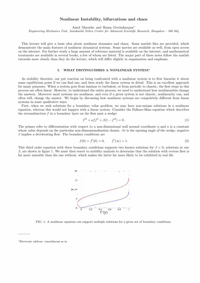
First, when we seek solutions for a boundary value problem, we may have non-unique solutions in a nonlinearequation, whereas this would not happen with a linear system. Consider the Falkner-Skan equation which describesthe streamfunction f in a boundary layer on the flow past a wedge:

f ′′′ + aff ′′ + β(1− f ′2) = 0. (1)

The primes refer to differentiation with respect to a non-dimensional wall normal coordinate η and a is a constantwhose value depends on the particular non-dimensionalisation chosen. βπ is the opening angle of the wedge, negativeβ implies a decelerating flow. The boundary conditions are

f(0) = f ′(0) = 0, f ′(∞) = 1. (2)

This third order equation with three boundary conditions supports two known solutions for β < 0, solutions at oneβ, are shown in figure 1. We must then resort to stability analysis to determine that the solution with reverse flow isfar more unstable than the one without, which makes the latter far more likely to be exhibited in real life.

FIG. 1: A nonlinear equation can support multiple solutions for a given set of boundary conditions.

∗Electronic address: rama@jncasr.ac.in

2

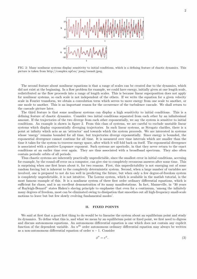
FIG. 2: Many nonlinear systems display sensitivity to initial conditions, which is a defining feature of chaotic dynamics. Thispicture is taken from http://complex.upf.es/ josep/rsensit.jpeg.

The second feature about nonlinear equations is that a range of scales can be created due to the dynamics, whichdid not exist at the beginning. In a flow problem for example, we could have energy, initially given at one length scale,redistributed as the flow proceeds into a range of length scales. This is because linear superposition does not applyfor nonlinear systems, so each scale is not independent of the others. If we write the equation for a given velocityscale in Fourier transform, we obtain a convolution term which serves to move energy from one scale to another, orone mode to another. This is an important reason for the occurrence of the turbulence cascade. We shall return tothe cascade picture later.

The third feature is that some nonlinear systems can display a high sensitivity to initial conditions. This is adefining feature of chaotic dynamics. Consider two initial conditions separated from each other by an infinitesimalamount. If the trajectories of the two diverge from each other exponentially, we say the system is sensitive to initialconditions. An example is shown in figure 2. From this class of systems, we are careful to exclude unstable linearsystems which display exponentially diverging trajectories. In such linear systems, as Strogatz clarifies, there is apoint at infinity which acts as an ‘attractor’ and towards which the system proceeds. We are interested in systemswhose ‘energy’ remains bounded for all time, but trajectories diverge exponentially. Since energy is bounded, theexponential divergence cannot continue for all time. It is measured over time intervals which are smaller than thetime it takes for the system to traverse energy space, after which it will fold back on itself. The exponential divergenceis associated with a positive Lyapunov exponent. Such systems are aperiodic, in that they never return to the exactconditions at an earlier time ever again. They are thus associated with a broadband spectrum. They also oftencontain periodic orbits of all periods.

Thus chaotic systems are inherently practically unpredictable, since the smallest error in initial conditions, accruingfor example, by the round-off error on a computer, can give rise to completely erroneous answers after some time. Thisis surprising when one first hears about it, for two reasons. First, this unpredictability is not emerging out of somerandom forcing but is inherent to the completely deterministic system. Second, when a large number of variables areinvolved, one is prepared to not do too well in predicting the future, but when only a few degree-of-freedom systemis completely unpredictable, it is not intuitive. The Lorenz system, which is available in the matlab tutorial, is themost famous example of this. It is a nonlinear system of three first order ordinary differential equations, which issufficient for chaos, and is an excellent demonstration of its many manifestations. In fact, Manneville, in “30 yearsof Rayleigh-Benard” states Haken’s slaving principle to emphasise that even for a continuum, ‘among the infinitelymany degrees of freedom, most can be eliminated owing to dissipation that smoothes out all high-frequency small-scalemotions to leave but but few slowly evolving fundamental modes’.

II. FIXED POINTS

We said at first that a good first thing to do would be to linearise the system about an equilibrium point and studyits dynamics. To define what this is, and what we mean by an equilibrium point or fixed point, we first need to digressand discuss autonomous equations. An autonomous differential equation is one which does not contain any explicitfunction of the dependent variable. An nth order autonomous ordinary differential equation may always be writtenas a non-autonomous differential equation of order n− 1. Consider

φ′′ = eφ. (3)

3

FIG. 3: A center, a saddle, a stable node, and a stable spiral. This picture is generated by using pplane.m, a free matlab code.

Substituting γ = φ′, we have φ′′ = γdγ/dφ, which may be integrated to give

12φ′2 = eφ + c, (4)

whose solution can be written down. The converse is also true, since a nonautonomous system in an array x, of theform

x = f(x, t) (5)

becomes an autonomous system if we include another equation t = 1. We therefore discuss autonomous systems atsome length. Their dynamics may be discussed in phase space, on whose axes are x and its n− 1 derivatives. If thesystem contains fixed points x0, where x = 0, we linearise the system about such a point by writing x = x0 + εx1 + ...for small ε, and neglect higher powers of ε to get a linear system

x1 = J0x1, (6)

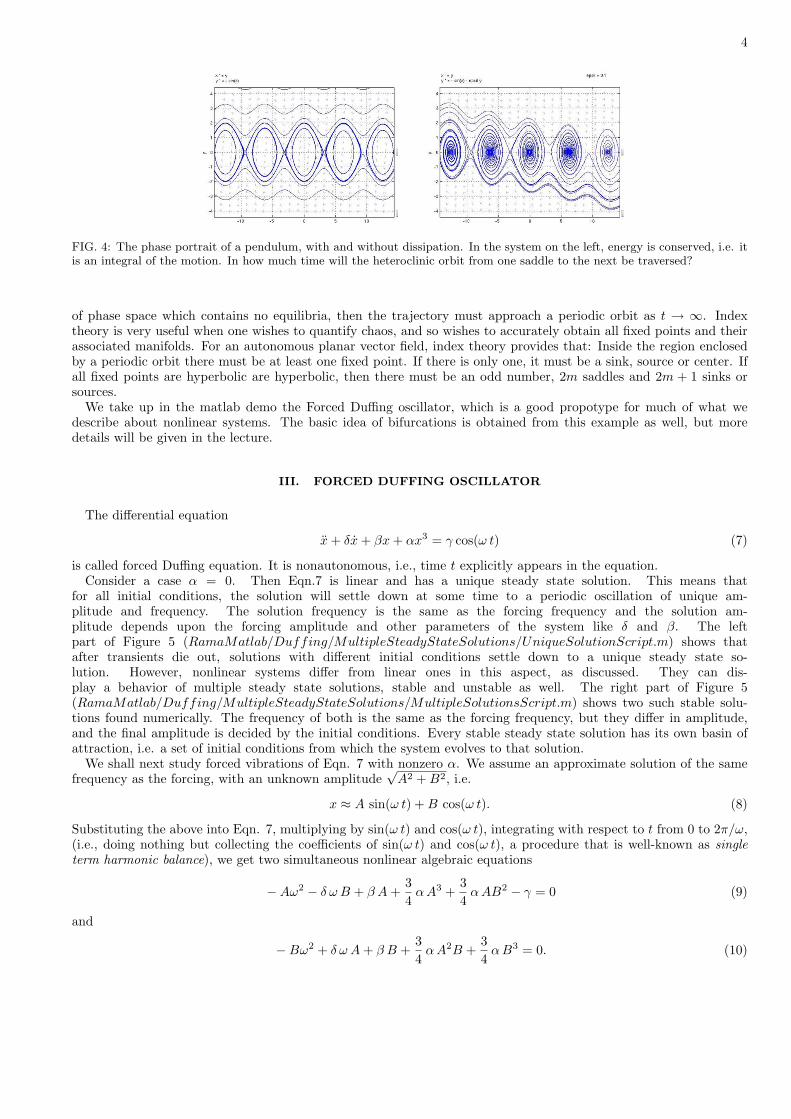
where J0, the Jacobian evaluated at x0, is a constant matrix. The real parts of the eigenvalues of J0 determinewhether the system is stable or unstable. If all real parts are negative, the system is stable, and the fixed pointwould be described by either a stable spiral or a stable node. If all eigenvalues have positive real parts, we haveunstable spirals or nodes, as will be seen by operating pplane.m, which is a freely downloadable code, included in thematlab tutorial. A fixed point is called a center if the real parts of the eigenvalues are 0. A saddle results when someeigenvalues are stable and the others unstable. Sample figures are shown in figure 3. We do not discuss degeneratecases here, but those are interesting as well. Near hyperbolic fixed points, i.e., those whose eigenvalues have non-zeroreal parts, the local phase portrait of the nonlinear system is topologically equivalent to that of the linear system.There is a homeomorphism from one to the other, as the Hartman-Grossman theorem assures us. So a hyperbolicfixed point is structurally stable whereas a centre is not. A small perturbation can change its nature, for example,a small dissipation will make it a stable spiral. A hyperbolic fixed point then has invariant manifolds associatedwith it. An invariant manifold of a fixed point is an orbit of a initial element in the flow starting out in one of theeigendirections of the fixed point. An element on a stable manifolds approaches the fixed point as t→∞, while thaton an unstable manifold approaches it in negative time, as t→ −∞. A heteroclinic orbit is one which originates fromone fixed point and terminates in another, while a homoclinic orbit is one which returns to the same fixed point att→∞. In this context, consider the dynamics of a simple pendulum, shown in figure 4.

The discussion on fixed points would be incomplete without mention of the Poincare-Bendixon theorem, and ofIndex theory. We quote from Guckenheimer and Holmes (1983) in the words of Jeff Moehlis in scholarpedia. Poincare-Bendixson Theorem: If a trajectory, in an autonomous system, enters and does not leave a closed and bounded region

4

FIG. 4: The phase portrait of a pendulum, with and without dissipation. In the system on the left, energy is conserved, i.e. itis an integral of the motion. In how much time will the heteroclinic orbit from one saddle to the next be traversed?

of phase space which contains no equilibria, then the trajectory must approach a periodic orbit as t → ∞. Indextheory is very useful when one wishes to quantify chaos, and so wishes to accurately obtain all fixed points and theirassociated manifolds. For an autonomous planar vector field, index theory provides that: Inside the region enclosedby a periodic orbit there must be at least one fixed point. If there is only one, it must be a sink, source or center. Ifall fixed points are hyperbolic are hyperbolic, then there must be an odd number, 2m saddles and 2m + 1 sinks orsources.

We take up in the matlab demo the Forced Duffing oscillator, which is a good propotype for much of what wedescribe about nonlinear systems. The basic idea of bifurcations is obtained from this example as well, but moredetails will be given in the lecture.

III. FORCED DUFFING OSCILLATOR

The differential equation

x+ δx+ βx+ αx3 = γ cos(ω t) (7)

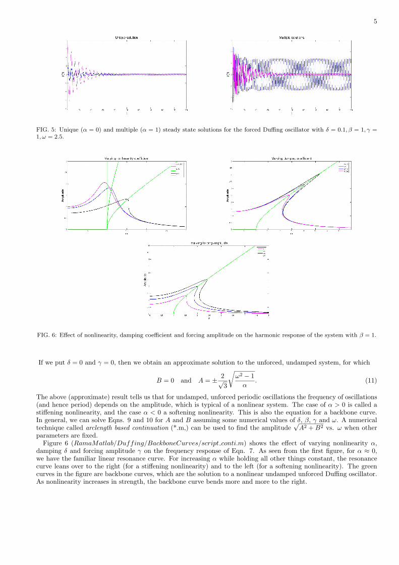
is called forced Duffing equation. It is nonautonomous, i.e., time t explicitly appears in the equation.Consider a case α = 0. Then Eqn.7 is linear and has a unique steady state solution. This means that

for all initial conditions, the solution will settle down at some time to a periodic oscillation of unique am-plitude and frequency. The solution frequency is the same as the forcing frequency and the solution am-plitude depends upon the forcing amplitude and other parameters of the system like δ and β. The leftpart of Figure 5 (RamaMatlab/Duffing/MultipleSteadyStateSolutions/UniqueSolutionScript.m) shows thatafter transients die out, solutions with different initial conditions settle down to a unique steady state so-lution. However, nonlinear systems differ from linear ones in this aspect, as discussed. They can dis-play a behavior of multiple steady state solutions, stable and unstable as well. The right part of Figure 5(RamaMatlab/Duffing/MultipleSteadyStateSolutions/MultipleSolutionsScript.m) shows two such stable solu-tions found numerically. The frequency of both is the same as the forcing frequency, but they differ in amplitude,and the final amplitude is decided by the initial conditions. Every stable steady state solution has its own basin ofattraction, i.e. a set of initial conditions from which the system evolves to that solution.

We shall next study forced vibrations of Eqn. 7 with nonzero α. We assume an approximate solution of the samefrequency as the forcing, with an unknown amplitude

√A2 +B2, i.e.

x ≈ A sin(ω t) +B cos(ω t). (8)

Substituting the above into Eqn. 7, multiplying by sin(ω t) and cos(ω t), integrating with respect to t from 0 to 2π/ω,(i.e., doing nothing but collecting the coefficients of sin(ω t) and cos(ω t), a procedure that is well-known as singleterm harmonic balance), we get two simultaneous nonlinear algebraic equations

−Aω2 − δ ω B + β A+34αA3 +

34αAB2 − γ = 0 (9)

and

−Bω2 + δ ω A+ β B +34αA2B +

34αB3 = 0. (10)

5

FIG. 5: Unique (α = 0) and multiple (α = 1) steady state solutions for the forced Duffing oscillator with δ = 0.1, β = 1, γ =1, ω = 2.5.

FIG. 6: Effect of nonlinearity, damping coefficient and forcing amplitude on the harmonic response of the system with β = 1.

If we put δ = 0 and γ = 0, then we obtain an approximate solution to the unforced, undamped system, for which

B = 0 and A = ± 2√3

√ω2 − 1α

. (11)

The above (approximate) result tells us that for undamped, unforced periodic oscillations the frequency of oscillations(and hence period) depends on the amplitude, which is typical of a nonlinear system. The case of α > 0 is called astiffening nonlinearity, and the case α < 0 a softening nonlinearity. This is also the equation for a backbone curve.In general, we can solve Eqns. 9 and 10 for A and B assuming some numerical values of δ, β, γ and ω. A numericaltechnique called arclength based continuation (*.m,) can be used to find the amplitude

√A2 +B2 vs. ω when other

parameters are fixed.Figure 6 (RamaMatlab/Duffing/BackboneCurves/script conti.m) shows the effect of varying nonlinearity α,

damping δ and forcing amplitude γ on the frequency response of Eqn. 7. As seen from the first figure, for α ≈ 0,we have the familiar linear resonance curve. For increasing α while holding all other things constant, the resonancecurve leans over to the right (for a stiffening nonlinearity) and to the left (for a softening nonlinearity). The greencurves in the figure are backbone curves, which are the solution to a nonlinear undamped unforced Duffing oscillator.As nonlinearity increases in strength, the backbone curve bends more and more to the right.

6

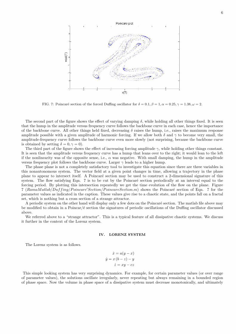
FIG. 7: Poincare section of the forced Duffing oscillator for δ = 0.1, β = 1, α = 0.25, γ = 1.38, ω = 2.

The second part of the figure shows the effect of varying damping δ, while holding all other things fixed. It is seenthat the hump in the amplitude versus frequency curve follows the backbone curve in each case, hence the importanceof the backbone curve. All other things held fixed, decreasing δ raises the hump, i.e., raises the maximum responseamplitude possible with a given amplitude of harmonic forcing. If we allow both δ and γ to become very small, theamplitude-frequency curve follows the backbone curve even more slowly (not surprising, because the backbone curveis obtained by setting δ = 0, γ = 0).

The third part of the figure shows the effect of increasing forcing amplitude γ, while holding other things constant.It is seen that the amplitude versus frequency curve has a hump that leans over to the right; it would lean to the leftif the nonlinearity was of the opposite sense, i.e., α was negative. With small damping, the hump in the amplitudeversus frequency plot follows the backbone curve. Larger γ leads to a higher hump.

The phase plane is not a completely satisfactory tool to investigate this equation since there are three variables inthis nonautonomous system. The vector field at a given point changes in time, allowing a trajectory in the phaseplane to appear to intersect itself. A Poincare section may be used to construct a 2-dimensional signature of thissystem. The flow satisfying Eqn. 7 is to be cut by the Poincare section periodically at an interval equal to theforcing period. By plotting this intersection repeatedly we get the time evolution of the flow on the plane. Figure7 (RamaMatlab/Duffing/Poincare′Section/PoincareSection.m) shows the Poincare section of Eqn. 7 for theparameter values as indicated in the caption. These values give rise to a chaotic state, and the points fall on a fractalset, which is nothing but a cross section of a strange attractor.

A periodic system on the other hand will display only a few dots on the Poincare section. The matlab file above maybe modified to obtain in a Poincar/e section the signatures of periodic oscillations of the Duffing oscillator discussedabove.

We referred above to a “strange attractor”. This is a typical feature of all dissipative chaotic systems. We discussit further in the context of the Lorenz system.

IV. LORENZ SYSTEM

The Lorenz system is as follows.

x = a(y − x)y = x (b− z)− y

z = xy − cz

This simple looking system has very surprising dynamics. For example, for certain parameter values (or over rangeof parameter values), the solutions oscillate irregularly, never repeating but always remaining in a bounded regionof phase space. Now the volume in phase space of a dissipative system must decrease monotonically, and ultimately

7

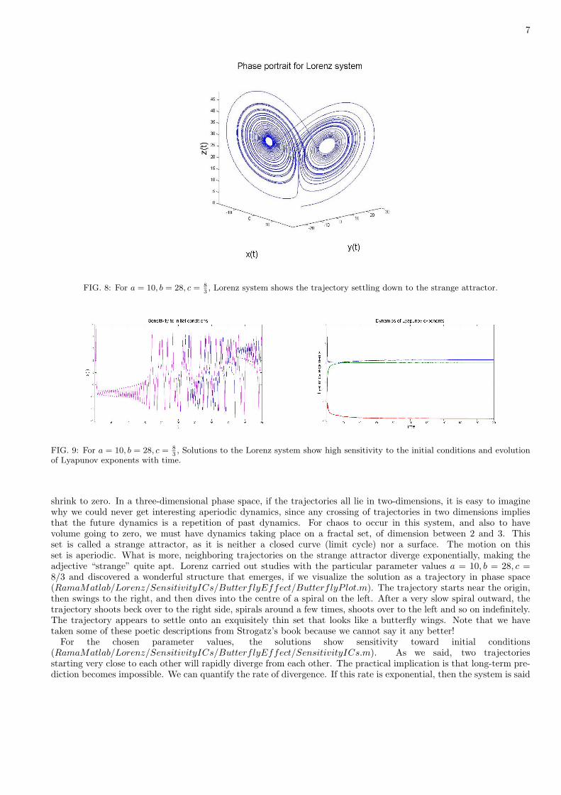
FIG. 8: For a = 10, b = 28, c = 83, Lorenz system shows the trajectory settling down to the strange attractor.

FIG. 9: For a = 10, b = 28, c = 83, Solutions to the Lorenz system show high sensitivity to the initial conditions and evolution

of Lyapunov exponents with time.

shrink to zero. In a three-dimensional phase space, if the trajectories all lie in two-dimensions, it is easy to imaginewhy we could never get interesting aperiodic dynamics, since any crossing of trajectories in two dimensions impliesthat the future dynamics is a repetition of past dynamics. For chaos to occur in this system, and also to havevolume going to zero, we must have dynamics taking place on a fractal set, of dimension between 2 and 3. Thisset is called a strange attractor, as it is neither a closed curve (limit cycle) nor a surface. The motion on thisset is aperiodic. What is more, neighboring trajectories on the strange attractor diverge exponentially, making theadjective “strange” quite apt. Lorenz carried out studies with the particular parameter values a = 10, b = 28, c =8/3 and discovered a wonderful structure that emerges, if we visualize the solution as a trajectory in phase space(RamaMatlab/Lorenz/SensitivityICs/ButterflyEffect/ButterflyP lot.m). The trajectory starts near the origin,then swings to the right, and then dives into the centre of a spiral on the left. After a very slow spiral outward, thetrajectory shoots beck over to the right side, spirals around a few times, shoots over to the left and so on indefinitely.The trajectory appears to settle onto an exquisitely thin set that looks like a butterfly wings. Note that we havetaken some of these poetic descriptions from Strogatz’s book because we cannot say it any better!

For the chosen parameter values, the solutions show sensitivity toward initial conditions(RamaMatlab/Lorenz/SensitivityICs/ButterflyEffect/SensitivityICs.m). As we said, two trajectoriesstarting very close to each other will rapidly diverge from each other. The practical implication is that long-term pre-diction becomes impossible. We can quantify the rate of divergence. If this rate is exponential, then the system is said

8

FIG. 10: Bifurcation diagram for logistic map.

to be chaotic for the chosen parameter values. The rate of exponential divergence is quantified in terms of Lyapunovexponents. Roughly speaking, the Lyapunov exponents measure the exponential growth or decay at time t, of aninitially spherical object in phase space, along its pricipal axes. An n-dimensional system will thus have n Lyapunovexponents. If the largest is greater than zero, then the system is chaotic. The time evolution of Lyapunov exponentsfor the chosen parameter values can be seen from Figure 9 (RamaMatlab/Lorenz/LorenzLyapunov/run lyap.m).

V. LOGISTIC MAP

We now briefly discuss the famous Logistic map, given by

xn+1 = µxn(1− xn). (12)

Suppose we fix the value of µ anywhere between 1 and 3 and iterate the map several times, a particular steady stateis reached. For a slightly larger value of µ say, 3.3, the final state of the sytem is one that oscillates between twovalues of x, we call this a period-2 cycle. If we increase µ further, we reach a point where the system oscillates; notbetween two, but between four values. This is called a period-4 cycle. As we keep increasing µ, such period-doublingskeep happening at closer and closer intervals of µ. If we denote by µn the value of the parameter µ where a 2n cyclefirst appears, then we get

δ = limn→∞

µn − µn−1

µn+1 − µn= 4.669.

This number appears in many kinds of maps, was discovered by Figenbaum, and carries his name. It is an importantnumber in the period doubling route to chaos. The implication is that at a finite value of µ, i.e., at µ = µ∞ ≈ 3.57, themap becomes chaotic. This route to chaos is thus a set of period-doubling bifurcations. If we plot the steady statesagainst parameter µ, we get the bifurcation diagram as shown in Figure 10 (RamaMatlab/Logisticmap/bdlogis.m).It will be noticed that there are periodic orbits in certain ranges of the parameter within the chaotic regime. Thisfeature too is ubiquitous in chaotic systems.

ConclusionsWe have tried to provide a short introduction to why nonlinear systems are interesting. We encourage the reader

to modify the matlab codes to obtain a variety of dynamics. The codes are all very short. In fact several of themhave only one or two operative lines.

Main references:

Bender C.M, Orszag S.A. 1999. Advanced Mathematical Methods for Scientists and Engineers I: Asymptotic Methodsand Perturbation Theory. Springer

Strogatz S.H. 2001. Nonlinear Dynamics and Chaos. Westview Press

9

Wiggins S. 2003. Introduction to Applied Nonlinear Dynamical Systems and Chaos. Springer

Rand R. Lecture Notes on Nonlinear Vibrations. Cornell University. audiophile.tam.cornell.edu/randdocs/-nlvibe52.pdf

Guckenheimer J, Holmes P. 1983. Nonlinear Oscillations, Dynamical Systems, and Bifurcations of Vector Fields.Springer

Lichtenberg A.J, Lieberman M.A. 1992. Regular and Chaotic Dynamics. Springer

Ott E. 1993. Chaos in Dynamical Systems. Cambridge University Press

www.scholarpedia.org

Anindya Chatterjee, matlab notes and programs

Many others