1

Nonparametric Measures of Economies of Scope

Alfons Oude Lansink and Spiro E. Stefanou

Revised 25 October 2006 Abstract: Measuring economies of scope provides a tool for explaining and predicting trends towards specialization or diversification within sectors like agriculture and horticulture. Focusing on nonparametric measurement and decomposition of scope economies into pure economies of scope, allocative efficiency, congestion efficiency and pure technical efficiency, an application to a sample of Dutch cash crop farms over the period 1995-1999 is the empirical focus. The results show that the potential economies of scope are lowered largely by allocative inefficiency and to a lesser extent by congestion inefficiencies and technical inefficiency, and the contraction impact of the various sources of inefficiencies drive these farms, on average, well into the diseconomies of scope range. The economic losses associated with allocative, congestion and technical inefficiencies lead to the potential to reduce costs by 25%, 7% and 6%, respectively. An analysis of results of diversified vis-à-vis specialized farms shows that policies should enhance particularly small and cereal farms to diversify. Also, increases of prices of pesticides and fertilizer substantially reduce the potential for cost savings from diversification. Hence fertilizer and pesticide taxes may have a large impact on the decisions of farmers to either diversify or specialize. This study also finds that capital is shareable factors of production, while labor and land are not.

* Alfons Oude Lansink is professor of Business Economics at Wageningen University (The Netherlands). Spiro E. Stefanou is professor of agricultural economics at Pennsylvania State University. Spiro E. Stefanou acknowledges the support of the Marie Curie Transfer of Knowledge Fellowship of the European Community's Sixth Framework Program at the Department of Economics at the University of Crete under contract number MTKD-CT-014288 during Spring 2006.

2

Nonparametric Measures of Economies of Scope The theory of multiple outputs/multiple inputs is relevant in the conceptualization of

resource allocation throughout the economy. Few important real-world analyses of

production or marketing operations (in the agri-food complex or elsewhere) are single

product in nature. A complete understanding of multiple output production decisions

requires developing meaningful technological specifications and measures reflecting the

potential for multiple output decisions. The consideration on non-jointness in production

decisions has preoccupied economists for the last half century starting with Carlson's

1939 classic study (reprinted 1965, pp. 74-102,) and Frisch (reprinted 1965, pp. 269-281)

who initiated close attention to the relation of nonjoint technology to total costs refined

by others [e.g., Mundlak (1964), Samuelson (1966), Lau (1972), Hall (1973), Hasenkamp

(1976), Kohli (1983), Mittelhammer et al. (1981), Shumway et al.(1984)]. Panzar and

Willig (1977) and Baumol, Panzar and Willig (1982) introduced the notion of multiple

output scale and scope to characterize the effects of size and output diversification for the

firm producing more than one output. Measuring economies of scale and scope is

essential to understanding the forces influencing structural, efficiency and productivity

changes.

The sources of jointness from both primal and dual perspectives are not always

transparent. Clearly, duality representations can preserve the jointness in technology and

present the manifestation of technological jointness in terms of cost, profit or revenue

[Lau (1978) among many others]. There are a myriad of forces unrelated to technological

jointness that can lead to the observation of joint production decisions as one investigates

behavior from the cost function perspective. One example of these forces include when

3

input quality cannot be easily distinguished in markets, the firm may decide to undertake

sourcing its inputs from its own production activity. Another example is when the

transportation price differences in sourcing inputs may lead to the cost minimizing

decision being to use own production of an input rather than purchasing the input on the

market. And, when firms have the ability to differentiate their products to extract greater

rents, they may look to maintain this advantage by pursuing a marketing strategy to

develop a platform of complementary products and services.

Olesen (1995) reviews the potential of DEA approaches to address issues related

to multiple output production and identifies the need to define indicators which can

inform the analyst of the degree the estimated technology is a joint technology. He

equates the economies of jointness with economies of scope and concludes that while

DEA can always provide an estimation of the multiple output technology, there are no

indicators available to advise the analyst whether or not the structure of the data supports

the existence of a joint technology. While this is the case for nonparametric analyses,

there have been econometric efforts focusing on the empirical determination of the

presence of jointness [e.g., Just et al. (1983), Shumway (1983), Chambers and Just

(1989), Fernandez-Cornejo et al (1992)]. Chavas and Aliber (1993) investigate scope

and efficiency in Wisconsin dairy farms following a nonparametric framework and find

that positive economies of scope exist for a variety of farm sizes, albeit it decreases for

significantly larger operations. In addition, they find that economic losses do result from

allocative and scale inefficiencies.

Färe, Groskopf and Lovell (1994, pp. 263-69) present a nonparametric framework

to compute the gains from combinations of farms and the diversification of products,

4

where diversification is characterized by farms of different types embodying different

cost functions. Delineating between specialized and diversified technologies, the

measure of the gains from diversification is the ratio of the sum of diversification to the

cost of producing all products together. This measure is in subtle contrast to Hall (1973)

[and elaborated on by Baumol, Panzar and Willig (1982)], which compares the cost of

operating separately to the cost of operating jointly, and necessarily maintains the

presence of a common cost (or production) structure. Färe, Grosskopf and Lovell create

a pseudo set of (or subsets of actual) specialized and diversified farms by building upon

the frontier performance. As such, this measure presents the potential gains from

diversification as the hypothetically diversified farms are constructed.

Measuring economies of scope facilitates the assessment of the benefits from

output diversification versus specialization for farms in a sector and provides a metric for

explaining and predicting trends towards specialization or diversification. However, this

measurement alone provided no insight into the potential trade off between the benefits of

diversification and the presence of suboptimal behavior in production decision making.

To remedy this shortcoming, this paper develops a measure of Total Economies of Scope

measuring the benefits of diversification and then decomposes this measure into Pure

Economies of Scope, allocative efficiency, congestion efficiency and pure technical

efficiency.

The decomposition of the nonparametric measure of Total Economies of Scope is

presented in the next section. This is followed by an empirical investigation of Dutch

cash crop farms, covering the period 1995-1999 where up to three outputs (rootcrops,

cereals and other outputs) and six inputs (i.e. pesticides, fertilizers, other variable inputs,

5

land, labor and capital) are distinguished. This empirical investigation explores the

causes of scope economies and their impact on the production structure.

Non-parametric Measures of Scope

The decomposition of economies of scope requires a measure reflecting the benefits of

joint production vis-à-vis production in separate production units. Baumol, Panzar and

Willig (1982) and Panzar and Willig (1977) propose a measure of economies of scope

using cost functions. Assuming a farm is minimizing costs of variable inputs (x) used to

produce a bundle of outputs, minimum costs to produce the output bundle y given fixed

inputs z and variable input prices w are given by the cost function C(y,w,z), defined as

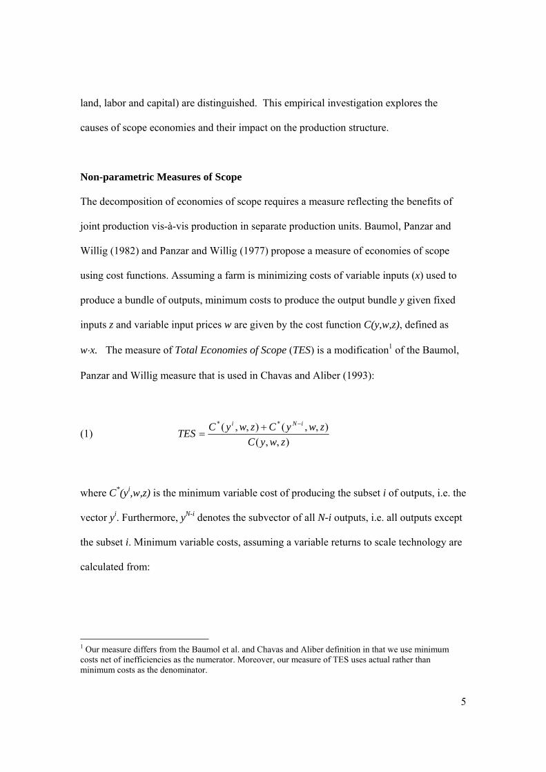
w⋅x. The measure of Total Economies of Scope (TES) is a modification1 of the Baumol,

Panzar and Willig measure that is used in Chavas and Aliber (1993):

(1) ),,(

),,(),,( **

zwyCzwyCzwyCTES

iNi −+=

where C*(yi,w,z) is the minimum variable cost of producing the subset i of outputs, i.e. the

vector yi. Furthermore, yN-i denotes the subvector of all N-i outputs, i.e. all outputs except

the subset i. Minimum variable costs, assuming a variable returns to scale technology are

calculated from:

1 Our measure differs from the Baumol et al. and Chavas and Aliber definition in that we use minimum costs net of inefficiencies as the numerator. Moreover, our measure of TES uses actual rather than minimum costs as the denominator.

6

(2)

01'1000

0..

min

*

**

≥=≥−

≥−≥

≥+−

⋅

−

λλλ

λλ

λ

NXxZz

YYy

ts

xw

iN

ii

x

Where x* denote cost minimizing quantities of variables inputs; Y (X,Z) is a vector of

observed outputs (variable inputs, fixed inputs) of all firms in the sample; λ is a vector of

weights that are positive for firms on the frontier and zero otherwise; N1 denotes an

(NxN) identity matrix. C*(yN-i,w,z) are minimum variable costs of producing the subvector

N-i of outputs given fixed inputs z and variable input prices w that are calculated from:

(3)

01'1

00

00

..

min

*

**

≥=≥−

≥−≥

≥+−

⋅

−−

λλλ

λλ

λ

NXx

ZzY

Yyts

xw

i

iNiN

x

TES can be defined as the product of pure economies of scope (PES) and overall

efficiency (OE), OEPESTES ⋅= :

(4) ),,(),,(

),,(),,(),,(

),,(),,(),,( *

*

****

zwyCzwyC

zwyCzwyCzwyC

zwyCzwyCzwyC iNiiNi

⋅+

=+ −−

7

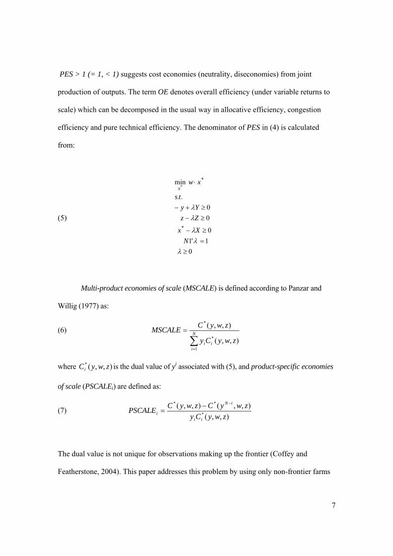
PES > 1 (= 1, < 1) suggests cost economies (neutrality, diseconomies) from joint

production of outputs. The term OE denotes overall efficiency (under variable returns to

scale) which can be decomposed in the usual way in allocative efficiency, congestion

efficiency and pure technical efficiency. The denominator of PES in (4) is calculated

from:

(5)

01'10

00

..

min

*

**

≥=≥−

≥−≥+−

⋅

λλλ

λλ

NXx

ZzYy

ts

xwx

Multi-product economies of scale (MSCALE) is defined according to Panzar and

Willig (1977) as:

(6) ∑=

= N

iii zwyCy

zwyCMSCALE

1

*

*

),,(

),,(

where ),,(* zwyCi is the dual value of yi associated with (5), and product-specific economies

of scale (PSCALEi) are defined as:

(7) ),,(

),,(),,(*

**

zwyCyzwyCzwyCPSCALE

ii

iN

i

−−=

The dual value is not unique for observations making up the frontier (Coffey and

Featherstone, 2004). This paper addresses this problem by using only non-frontier farms

8

for the computation of scale economies (6) and the indicator for product-specific inputs

(7).

Data

Data on specialized cash crop farms covering the period 1995-1999 come from a stratified

sample of Dutch farms in the accounting system of the Agricultural Economics Research

Institute (LEI). The farms typically remain in the panel for a maximum of five to eight years

leading to an incomplete panel. Farms are replaced in the sample to avoid a selection bias,

which arises when farms improve their performance by their presence in the accounting

system.

Three outputs (cereals, rootcrops and other outputs) and six inputs (pesticides,

fertilizers, other variable inputs, land, labor and capital) are distinguished. Variable inputs

are pesticides, fertilizers and other variable inputs. Cereals include wheat, barley and oats;

other outputs are mainly protein crops, vegetables and other crops. Rootcrops (mainly

potatoes and sugar beet) are the main source of income for most cash crop farms in the

Netherlands. The typical crop rotation of specialized cash crop farms consists of potatoes

sugar beet, cereals and one other crop. Four observations report zero output for rootcrops;

118 for cereals and 123 for other outputs. Two farm types are distinguished in the sample,

with rootcrop farms defined as farms with an above average (36%) share of revenues

from rootcrops in total revenues; the other farms are denoted as cereal production-

oriented enterprises. The data sets used for the estimations contain 527 and 764 observati-

ons on rootcrop-oriented farms and cereal-oriented farms, respectively (the total number of

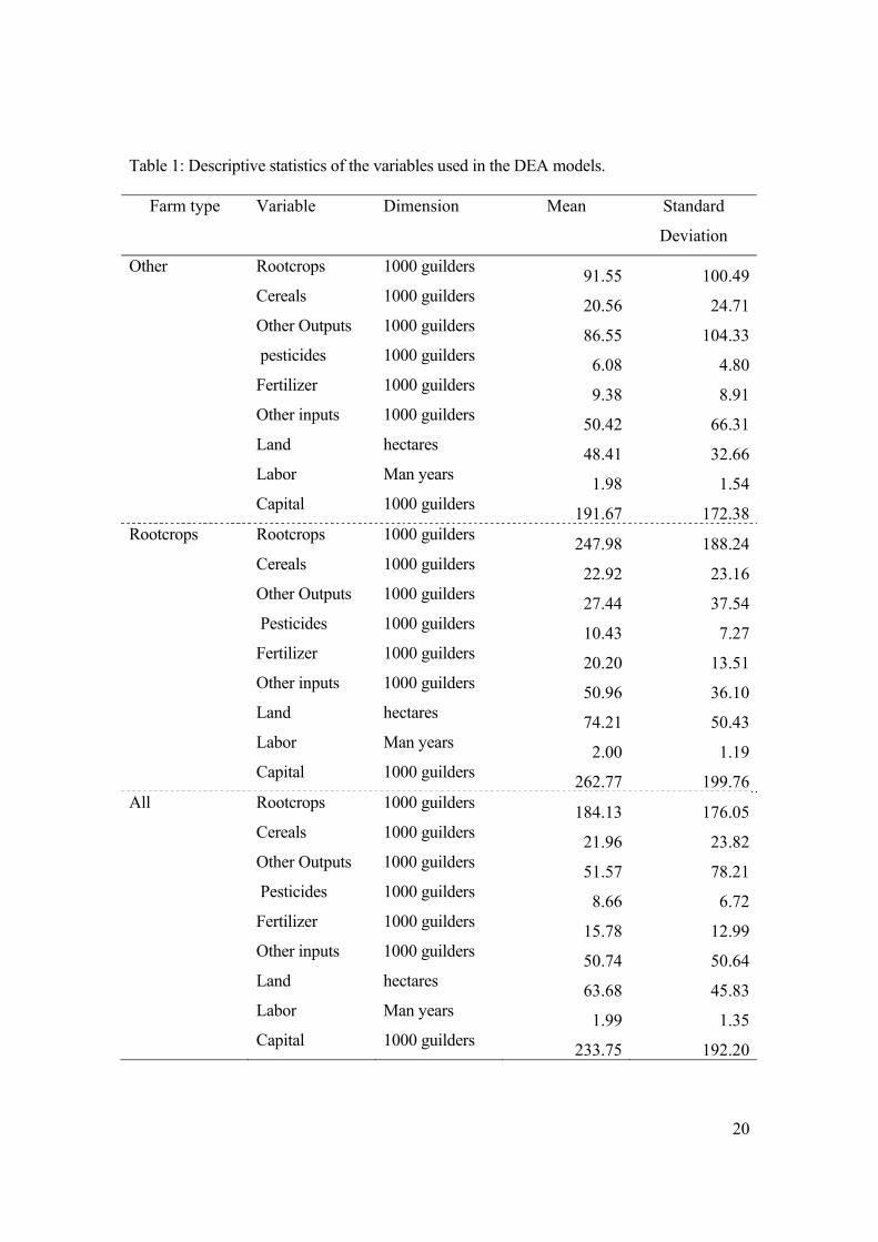
observations is 1291). A detailed description of the data can be found in Table 1.

9

Fixed inputs are land, labor and capital. Land is measured in hectares; labor is

measured in quality-corrected man years, and includes family as well as hired labor. In this

study, labor is assumed to be a fixed input since a large share of total labor consists of family

labor. Flexibility of hired labor is further restricted by the presence of permanent contracts

and by the fact that hiring additional labor involves search costs for the farm operator. 2 The

quality correction of labor is performed by the LEI and is necessary to aggregate labor

from able-bodied adults with labor supplied by young people (e.g., young family

members) or partly disabled workers. Capital reflects replacement costs3 of buildings,

machinery and installations and is measured at constant 1995 prices.

Implicit quantity indexes are generated as the ratio of value to the price index.

Tornqvist price indexes are calculated for the composite outputs and variable inputs with

prices obtained from the LEI and Central Bureau of Statistics (LEI/CBS). The price

indexes vary over the years but not over the farms, implying differences in the

composition of inputs and output or quality differences are reflected in the quantity (Cox

and Wohlgenant, 1986).

2 As table 1 indicates, the average man-years for total labor is under 2, suggesting hired labor is a small part of the variable input decisions process. 3 The deflators for capital in structures and machinery and installations are calculated from the data supplied by the LEI accounting system. Comparison of the balance value in year t and the balance value in year t-1 gives the yearly price correction used by the LEI. This price correction is used to construct a price index for capital and a price index for buildings, machinery and installations. These price indices are used as deflators.

10

Results

Solutions for the mathematical programming problems in (2), (3) and (5) are obtained

using GAMS. The models are run for each farm in the sample in each year, using all

other farms in the sample in the same year as reference group. Total Economies of Scope

(TES) by farm type and year and its decomposition into Pure Economies of Scope (PES),

allocative, congestion and pure technical efficiency are generated.4

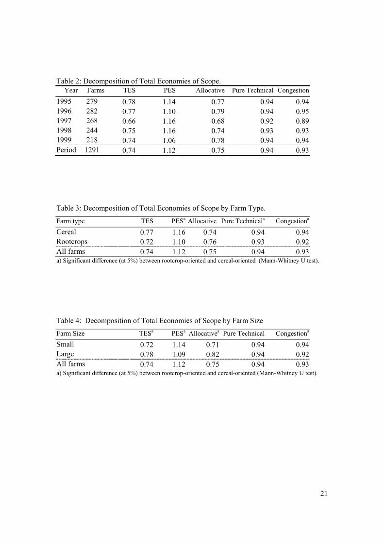
Tables 2 presents results indicating that the TES are in the range of 0.66-0.78,

while PES, on average, are greater than unity for all years suggesting that the farms in

the sample face lower total costs when producing more than one output. Further,

allocative efficiency is the most important determinant of TES in all years, averaging in

the range of 0.68-0.79 in the period under investigation implying that the farms in the

sample could reduce their variable costs by 21 to 32 percent through an optimal re-

allocation of variable inputs. Pure technical inefficiency is the smallest component of

TES, with an average inefficiency of 6%. This is consistent with the Chavas and Aliber

findings that allocative inefficiency is relatively more severe than technical inefficiency.5

Congestion is the second most important contributor to inefficiency, as it can lead to a 7

percent reduction of the use of the variable inputs. Congestion is often caused by the

failure to adjust input quantities instantaneously, which is plausible for inputs like

pesticides and fertilizers. Their use is largely determined by the composition of the crop

mix which cannot change instantaneously. Changing the use of pesticides requires new

4 The decomposition into allocative, congestion and pure technical efficiency is demonstrated in Färe, Grosskopf and Lovell (1994) for details on the decomposition. 5 Chavas and Aliber (1993) generate both short run and long run efficiency estimates for nine different Wisconsin dairy production districts. For comparison in this study, the weighted group means are calculated from their Table 2, page 10, the short run measures for TE and AE are 0.93 and 0.83,

11

(e.g. resistant) crop varieties and new cultivation practices, replacing chemicals by

mechanical weeding. Similarly, applications of fertilizers like Potassium and Phosphates

are part of a multi-year crop plan.

Table 3 decomposes the Pure Economies of Scope and the efficiency components

of the cereal-oriented versus the rootcrop-oriented farms and reveals that on rootcrop-

oriented farms the total scope economies are slightly smaller indicating that these farms

have lower cost savings from joint production than cereal-oriented farms. A non-

parametric Mann-Whitney U test is employed to test for the significance of the

differences between farm types. The test results show that all differences between farm

types are significant at the 5% level for PES, congestion efficiency and pure technical

efficiency. The rootcrop-oriented farms generally have a lower score for these

components. The lower score for Pure Economies of Scope implies that rootcrop farms

achieve lower cost savings from joint production than the cereal-oriented farms.

Although both farm types benefit from diversification cereal oriented farms have a larger

incentive for joint production than rootcrop farms. This result may reflect the negative

impact of rootcrops on soil fertility, thereby partly undoing the benefits of joint

production. The lower congestion efficiency on rootcrop farms suggests that it is more

difficult for these farms to adjust the inputs instantaneously than for other farms. This

result is in line with the observation that sugar beet and potatoes are more intensively

using variable inputs (fertilizers and pesticides) than other crops.

In analyzing the relation between farm size and TES, for each farm type, a

category of small (large) farms is defined as those farms having a smaller (larger) land

respectively. The weighted mean for the measure of scope economies from the same table is 1.50; albeit this is a long run measure (no short run measure is reported).

12

area than the farm type’s average. When focusing on farm size, a different profile

emerges. While table 2 indicates that allocative inefficiency is the most important

determinant of TES, Table 4 indicates that smaller farms present a substantially greater

degree of allocative inefficiency and lesser degree of congestion inefficiency. Overall,

small and large farms present the same level of technical efficiency. On balance, smaller

farms have a higher Pure Economies of Scope measure but a smaller Total Economies of

Scope measure compared to larger farms. The higher Pure Economies of Scope measure

on small farms suggests that joint production is more beneficial on small farms than on

large farms. This suggests that part of the benefits of diversification is lost when

producing at a larger scale.

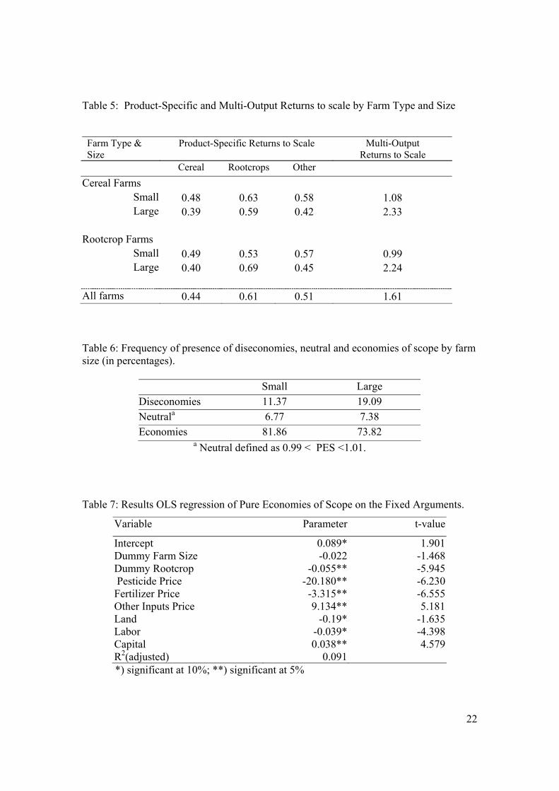
The product-specific components of multi-output returns to scale by farm size and

farm production orientation are presented in table 5. The product-specific returns to scale

is substantially in the decreasing returns to scale range when considering the single-

output perspective of production decision making, while the multi-output returns to scale

is in the constant or increasing returns to scale range. Cereal production presents the

lowest product-specific returns to scale in all cases, while rootcrop production presents

the highest product-specific returns to scale in all cases, except small rootcrop-oriented

farms. Farm size has the most significant impact on the multi-output returns to scale with

small farms at or close to the constant returns to scale production, and larger farms

exhibiting substantial increasing returns to scale. This suggests that regulatory or

infrastructure factors constrain the ability of larger farm operators to exploit economies of

scale6.

6 The economies of scale for large farms are larger than what is often found in the literature, but are in line with the findings of Abdullahi et al. (2006) for Kansas wheat and beef-cow operations. The large

13

The frequency distributions of the Pure Economies of Scope for the small and

large farms are both distributed normal.7 Table 6 presents the frequency of the presence

of negative, neutral and positive economies of scope for small and large farms, where the

indication of neutral economies of scope is generously interpreted as 1.0 ± .01. The small

farms present a greater frequency of positive scope economies, which is in line with the

finding of a higher average score for Pure Economies of Scope on small farms in Table 4.

Table 7 presents the results of the investigation of the forces impacting scope

economies with the presentation of a log-linear regression of Pure Economies of Scope on

three sets of explanatory variables. The first set comprises a set of dummies reflecting farm

production orientation (1, if rootcrop-oriented) and farm size (1, if large). The results

indicate that farms that are rootcrop-oriented or large will lower PES, ceteris paribus.8

There is a significant negative impact of the rootcrop-oriented farming operations on

scope economies which reflects the fact that crop rotation restrictions are constraining the

sharing of land across the production of different outputs more severe for rootcrop farms

rather than for other farms. This is because on rootcrop farms, the pressure of soil born

diseases is higher.

The second set of variables involves the variable input prices. The marginal impact

of a variable input price on the Pure Economies of Scope measure can be expressed into a

dimensionless measure by multiplying through by price to yield

economies of scale may also be associated with the nonparametric method that is used in this paper. The size of the economies of scale depends on derivatives at the frontier which may become very small or large. 7 The Komolgorov-Smirnoff test does not reject normal distributions of PES with a test statistic of 0.124 and 0.082 for small and large farms, respectively, both significant at < 0.001. Small farms have a sample mean of 1.14 and standard deviation of 0.198, while large farms have a sample mean of 1.09 and standard deviation of 0.152. 8 Dummy variables reflecting soil type and characteristics related to the farm operator (education, presence of a successor, and tenure status) did not contribute significantly to the explanatory power of the regression.

14

(9) [ ]intjoj

separatei

jj ssPES

wPESw −⋅=∂∂ ,

where ),,(),,(

),,(),,(** zwyCzwyC

zwyxwzwyxws iNi

iNjj

ijjseparate

j −

−

+

+= and

),,(),,(

*int

zwyCzwyxw

s jjjoj = , reflect the jth

input cost share of producing separately and jointly, respectively.

Price changes can lead to input substitutions that eventually impact costs of

production. The presence of economies (diseconomies) of scope magnifies (contracts) the

cost share differences. Table 7 shows that variable input price changes can have a

substantial impact on scope economies. Price increases in agricultural chemicals (pesticides

and fertilizers) have a negative impact on scope economies while a price increase for the

miscellaneous input variable enhances scope economies. The changes in input mixes driven

by relative price changes can have a substantial impact on the organization of these farms.

Pure Economies of Scope is highly elastic, ranging from 3.3 to 20 percent reduction in

scope economies from a one percent increase in the prices of fertilizer and pesticide,

respectively, to a 9 percent increase in scope economies from an increase in the

miscellaneous input variable.

The third set of variables comprises the fixed inputs in the production process.

Shared fixed inputs are fixed inputs used by several outputs in the production process;

output-specific fixed inputs are used for the production of specific outputs. The presence of

shared or output-specific fixed inputs is inferred from the impact on Pure Scope Economies

of increasing fixed inputs in the regression model.9 A positive (negative) impact of the fixed

9 A discrete approximation of the marginal impact can be achieved by:

2*

***

),,(),,(),,(),,(

zwyCzwyCzwyCzwyC

z

ziT

zi

z −+ − , where

),,(* zwyCz, ),,(* zwyC i

zand ),,(* zwyC iT

z− are the dual values associated with the constraint on the z-inputs in the cost

15

input on Pure Economies of Scope suggests the fixed input is a shared (product-specific)

fixed input. Results in Table 7 show that all three fixed factors have a significant impact

on PES, revealing a highly inelastic response with a 10 percent increase in capital and

labor leading to a less than 4 percent increase and decrease, respectively, in scope

economies The impact of land is negative suggesting increases in this asset will decrease

incentives for joint production, albeit it, at half the response in absolute value as the other

assets marginally. Thus, capital is a shared (or farm-specific) asset, on balance, while

labor and land are product-specific assets suggesting that no production expertise

spillovers are evident and that many of these cash crop farms rent land purely for growing

potatoes. There is a significant negative impact of the rootcrop-oriented farming

operations on scope economies which reflects the restrictions of crop rotation restrictions,

which facing higher pressure of soil borne diseases compared to other crop farms. In

contrast, Goodwin, Featherstone and Zeuli (2002) find a robust correlation between a

farm's historical yield on other crops and a newly produced crop when considering wheat,

corn and soybean production in Kansas.

Conclusion

Measuring economies of scope provides a tool for explaining and predicting trends

towards specialization or diversification within sectors like agriculture and horticulture.

This paper focuses on nonparametric measurement and decomposition of scope

minimization problems in (5), (2) and (3), respectively. However, corners on the surface can be encountered, leaving this an

unsuitable option.

16

economies into PES, allocative efficiency, congestion efficiency and pure technical

efficiency.

Results for a sample of Dutch cash crop farms over the period 1995-1999 show

that the potential economies of scope are lowered largely by allocative inefficiency and to

a lesser extent by congestion inefficiencies and technical inefficiency, and the contraction

impact of the various sources of inefficiencies drive these farms, on average, well into the

diseconomies of scope range. While the economic incentives for joint diversification

exist given the structure of production, the economic losses associated with allocative,

congestion and technical inefficiencies lead to the potential to reduce costs by 25%, 7%

and 6%, respectively. Rootcrop production-oriented farms and larger farms tend to have

lower (albeit, still positive) scope economies potential. This study also finds that capital

is a shareable factor of production, while labor and land are not.

Analysis of results of diversified vis-à-vis specialized farms shows that policies

should enhance particularly small and cereal farms to diversify. Also, increases of prices

of pesticides and fertilizer substantially reduce the potential for cost savings from

diversification. Hence fertilizer and pesticides taxes may have a large impact on the

decisions of farmers to either diversify or specialize.

17

References

Abdullahi, O.A., M. Langemeier and A.M. Featherstone (2006). Estimating Economies

of Scope and Scale under Price Risk and Risk Aversion. Applied Economics 38;

p191-201.

Agricultural Economics Research Institute and Central Bureau of Statistics (LEI/CBS,

various years) Landbouwcijfers, The Hague.

Baumol, W.J., J.C. Panzar and R.D. Willig (1982). Contestable Markets and the Theory of

Industry Structure. New York: Harcourt Brace Jovanovich, 1982.

Carlson, S. (1965). A study of the pure theory of production. Reprint of Economic Classics.

August. M. Kelley.

Chambers, R.G., R. Just (1989). “Estimating Multioutput Technologies.” American Journal of

Agricultural Economics, 71; 981-995.

Chavas, J.P. & Aliber, M. (1993). An analysis of economic efficiency in agriculture: a

nonparametric approach. Journal of Agricultural and Resource Economic, 18(1): 1-

16.

Coffey, B.K. and A. M. Featherstone (2004). “Nonparametric Estimation of Multiproduct and

Product-Specific Economies of Scale.” Selected paper presented at the Annual

Meetings of the Southern Agricultural Economics Association, Tulsa, OK.

Cox, T.L., M.K. Wohlgenant (1986). “Prices and Quality Effects in Cross-sectional

Demand Analysis.” American Journal of Agricultural Economics, 68, 908-919.

Färe, R., S. Grosskopf and C.A.K. Lovell (1994). Production Frontiers. New York:

Cambridge University Press.

Fernandez-Cornejo, J., C.M. Gempesaw II, J.G. Elterich, and S.E. Stefanou (1992).

“Dynamic Measures of Scope and Scale Economies: An Application to German

Agriculture.” American Journal of Agricultural Economics, 74; 329-342.

18

Frisch, R. Theory of Production. Chicago: Rand McNally and Company, 1965.

Goodwin, B.K., A.M. Featherstone, and K. Zeuli (2002). “Producer Experience,

Learning by Doing, and Yield Performance.” American Journal of Agricultural

Economics, 84: 660-78.

Hall, R. E. (1973). "The Specification of Technology with Several Kinds of Output."

Journal of Political Economy, 8l:878-892.

Hasenkamp, G. (1976). Specification and Estimation of Multiple Output Production

Functions. Lecture notes in Economics and Mathematical Systems, no. 120, Berlin:

Springer-Verlag.

Just, R.E., D. Zilberman and E. Hochman (1983). “Estimation of Multicrop Production

Functions.” American Journal of Agricultural Economics 65 (November): 770-

780.

Kohli, U. (1983). "Non-joint Technologies." Review of Economic Studies 50: 209-19.

Lau, L.J. (1972). "Profit Functions of Technologies with Multiple Inputs and Outputs."

Review of Economics and Statistics, 54:281-89.

Lau, L.J. (1978). “Applications of Profit Functions,” in M. Fuss and D.L. McFadden, eds.

Production Economics: A Dual Approach to Theory and Applications (Volume I:

The Theory of Production), Amsterdam: North-Holland, 1978, pp: 133-216.

Mittelhammer, R.C., S.C. Matulich and D. Bushaw (1981). "On Implicit Forms of

Multiproduct-Multifactor Production Functions." American Journal of

Agricultural Economics, 63:l64-l68.

Mundlak, Y. (1964) "Transcendental Multi-Product Production Functions."

International Economics Review, 5:273-284.

19

Olesen, O. B. (1995). “Some Unsolved Problems in Data Envelopment Analysis: A

Survey.” International Journal of Production Economics, Vol. 39, pp. 5-36.

Oude Lansink, A. and I. Bezlepkin (2003). “The Effect of Heating Technologies on CO2

and Energy Efficiency of Dutch Greenhouse Farms.” Journal of Environmental

Management 68: 73-82.

Panzar, J.C. and R.D. Willig (1977). “Economies of Scale in Multi-Output Production.”

Quarterly Journal of Economics, 91: 481-93.

Samuelson, P.A. (1966). "The Fundamental Singularity Theorem for Non-Joint

Production." International Economic Review, 7:34-41.

Shumway, C.R. (1983). “Supply, Demand And Technology in A Multiproduct Industry:

Texas Field Crops.” American Journal of Agricultural Economics, 65: 748-760.

Shumway, C. R., R. D. Pope and E. K. Nash (1984). "Locatable Fixed Inputs and

Jointness in Production: Implications for Economic Modeling." American Journal

of Agricultural Economics, 66:72-78.

20

Table 1: Descriptive statistics of the variables used in the DEA models.

Farm type Variable Dimension Mean Standard

Deviation

Other Rootcrops 1000 guilders 91.55 100.49 Cereals 1000 guilders 20.56 24.71 Other Outputs 1000 guilders 86.55 104.33 pesticides 1000 guilders 6.08 4.80 Fertilizer 1000 guilders 9.38 8.91 Other inputs 1000 guilders 50.42 66.31 Land hectares 48.41 32.66 Labor Man years 1.98 1.54 Capital 1000 guilders 191.67 172.38Rootcrops Rootcrops 1000 guilders 247.98 188.24 Cereals 1000 guilders 22.92 23.16 Other Outputs 1000 guilders 27.44 37.54 Pesticides 1000 guilders 10.43 7.27 Fertilizer 1000 guilders 20.20 13.51 Other inputs 1000 guilders 50.96 36.10 Land hectares 74.21 50.43 Labor Man years 2.00 1.19 Capital 1000 guilders 262.77 199.76All Rootcrops 1000 guilders 184.13 176.05 Cereals 1000 guilders 21.96 23.82 Other Outputs 1000 guilders 51.57 78.21 Pesticides 1000 guilders 8.66 6.72 Fertilizer 1000 guilders 15.78 12.99 Other inputs 1000 guilders 50.74 50.64 Land hectares 63.68 45.83 Labor Man years 1.99 1.35 Capital 1000 guilders 233.75 192.20

21

Table 2: Decomposition of Total Economies of Scope.

Year Farms TES PES Allocative Pure Technical Congestion

1995 279 0.78 1.14 0.77 0.94 0.94 1996 282 0.77 1.10 0.79 0.94 0.95 1997 268 0.66 1.16 0.68 0.92 0.89 1998 244 0.75 1.16 0.74 0.93 0.93 1999 218 0.74 1.06 0.78 0.94 0.94 Period 1291 0.74 1.12 0.75 0.94 0.93

Table 3: Decomposition of Total Economies of Scope by Farm Type.

Farm type TES PESa Allocative Pure Technicala Congestiona

Cereal 0.77 1.16 0.74 0.94 0.94 Rootcrops 0.72 1.10 0.76 0.93 0.92 All farms 0.74 1.12 0.75 0.94 0.93 a) Significant difference (at 5%) between rootcrop-oriented and cereal-oriented (Mann-Whitney U test).

Table 4: Decomposition of Total Economies of Scope by Farm Size

Farm Size TESa PESa Allocativea Pure Technical Congestiona

Small 0.72 1.14 0.71 0.94 0.94 Large 0.78 1.09 0.82 0.94 0.92 All farms 0.74 1.12 0.75 0.94 0.93 a) Significant difference (at 5%) between rootcrop-oriented and cereal-oriented (Mann-Whitney U test).

22

Table 5: Product-Specific and Multi-Output Returns to scale by Farm Type and Size

Farm Type & Size

Product-Specific Returns to Scale Multi-Output Returns to Scale

Cereal Rootcrops Other Cereal Farms

Small 0.48 0.63 0.58 1.08 Large 0.39 0.59 0.42 2.33

Rootcrop Farms

Small 0.49 0.53 0.57 0.99 Large 0.40 0.69 0.45 2.24

All farms 0.44 0.61 0.51 1.61

Table 6: Frequency of presence of diseconomies, neutral and economies of scope by farm size (in percentages).

Small Large Diseconomies 11.37 19.09 Neutrala 6.77 7.38 Economies 81.86 73.82

a Neutral defined as 0.99 < PES <1.01.

Table 7: Results OLS regression of Pure Economies of Scope on the Fixed Arguments.

Variable Parameter t-value

Intercept 0.089* 1.901 Dummy Farm Size -0.022 -1.468 Dummy Rootcrop -0.055** -5.945 Pesticide Price -20.180** -6.230 Fertilizer Price -3.315** -6.555 Other Inputs Price 9.134** 5.181 Land -0.19* -1.635 Labor -0.039* -4.398 Capital 0.038** 4.579 R2(adjusted) 0.091 *) significant at 10%; **) significant at 5%