notes on satellite meteorology - cooperative institute for
TRANSCRIPT

REMOTE SENSING APPLICATIONS
WITH
METEOROLOGICAL SATELLITES
by
W. Paul Menzel
University of Wisconsin
Madison, WI
November 2012
© 2012 W. Paul Menzel

2
These notes, compiled for classroom reading, are derived from discussions, collaborations, efforts, and papers of many colleagues, acquaintenances, and peers in the remote sensing
community.

3
TABLE OF CONTENTS Page
CHAPTER 1 - EVOLUTION OF SATELLITE METEOROLOGY
1.1 Before Satellites 8 1.2 Evolution of the Polar Orbiting Satellites 8 1.3 The Geostationary Program 14 1.4 Data Processing Capability 17 1.5 Impact of Satellite Data on NWP 18 1.6 Summary 19
CHAPTER 2 - NATURE OF RADIATION
2.1 Remote Sensing of Radiation 26 2.2 Basic Units 26 2.3 Definitions of Radiation 27 2.4 Historical Development of Planck's Radiation Law 29 2.5 Related Derivations 31 2.5.1 Wien’s Displacement Law 31 2.5.2 Rayleigh-Jeans Radiation Law 32 2.5.3 Wien’s Radiation Law 33 2.5.4 Stefan-Boltzmann Law 33 2.5.5 Brightness Temperature 34
CHAPTER 3 - ABSORPTION, EMISSION, REFLECTION, AND SCATTERING
3.1 Absorption and Emission 41 3.2 Conservation of Energy 41 3.3 Planetary Albedo 42 3.4 Selective Absorption and Emission 42 3.5 Absorption (Emission) Line Formation 44 3.6 Vibrational and Rotational Spectra 46 3.7 Summary of Interactions between Radiation and Matter 47 3.8 Beer's Law and Schwarzchild's Equation 48 3.9 Atmospheric Scattering 51 3.10 The Solar Spectrum 52 3.11 Composition of the Earth's Atmosphere 53 3.12 Atmospheric Absorption and Emission of Solar Radiation 53 3.13 Atmospheric Absorption and Emission of Thermal Radiation 54 3.14 Atmospheric Absorption Bands in the IR Spectrum 55 3.15 Atmospheric Absorption Bands in the Microwave Spectrum 56 3.16 Remote Sensing Regions 56
CHAPTER 4 - THE RADIATION BUDGET
4.1 The Mean Global Energy Balance 67 4.2 The First Satellite Experiment to Measure Net Radiation 67 4.3 The Radiation Budget 69 4.4 Distribution of Solar Energy Intercepted by the Earth 70 4.5 Solar Heating Rates 71 4.6 Infrared Cooling Rates 71 4.7 Radiative Equilibrium in a Gray Atmosphere 72

4
CHAPTER 5 - THE RADIATIVE TRANSFER EQUATION (RTE)
5.1 Derivation of RTE 78 5.2 Temperature Profile Inversion 82 5.3 Transmittance Determinations 83 5.4 Fredholm Form of RTE and Direct Linear Inversion 84 5.5 Linearization of the RTE 86 5.6 Statistical Solutions for the Inversion of the RTE 87
5.6.1 Statistical Least Squares Regression 87 5.6.2 Constrained Linear Inversion of RTE 87 5.6.3 Statistical Regularization 89 5.6.4 Minimum Information 90 5.6.5 Empirical Orthogonal Functions 90
5.7 Numerical Solutions for the Inversion of the RTE 95 5.7.1 Chahine Relaxation Method 95 5.7.2 Example Problem Using Relaxation Method 97 5.7.3 Smith's Iteration 99 5.7.4. Example Problem Using Smith's Iteration 100 5.7.5 Comparison of Chahine & Smith Iteration Solution 102
5.8 Direct Physical Solution 103 5.8.1 Solving Linear RTE Direct 103 5.8.2 Simultaneous Direct Physical Solution of the RTE 104
5.9 Water Vapor Profile Solutions 107 5.10 Microwave Form of RTE 108
CHAPTER 6 - DETECTING CLOUDS
6.1 RTE in Cloudy Conditions 113 6.2 Inferring Clear Sky Radiances in Cloudy Conditions 114 6.3 Finding Clouds 116 6.3.1 Threshold Tests for Finding Cloud 116
6.3.2 Spatial Uniformity Tests to Find Cloud 122 6.4 The Cloud Mask Algorithm 123
6.4.1 Thick High Clouds 124 6.4.2 Thin Clouds 124 6.4.3 Low Clouds 124 6.4.4 Thin High Clouds 125 6.4.5 Ancillary Data Requirements 125 6.4.6 Implementing the Cloud Mask Algorithms 126 6.4.7 Clear Sky Composite Maps 127
6.5 Cloud Properties Derived in a MODIS Granule 127 6.5.1 Cloud Masking 127 6.5.2 Cloud Thermodynamic Phase 128 6.5.3 Cloud Top Pressure and Effective Cloud Amount 129 6.5.4 Detection of UT/LS Clouds 129 6.5.5 Cloud Optical and Microphysical Properties 131 6.5.6 Detection of Multi-layerd Clouds 131 6.5.7 Global Gridded Products 132

5
6.6 Ongoing Cloud Climatologies 133
6.6.1 ISSCP 134 6.6.2 CLAVR 134 6.6.3 CO2 Slicing 135 6.6.4 UT/LS Clouds 137 6.6.5 Comparison of Cloud Amount in Global Climatologies 138
CHAPTER 7 - SURFACE TEMPERATURE
7.1 Sea Surface Temperature Determination 156 7.1.1 Slope Method 156 7.1.2 Three point Method 157 7.1.3 Least Squares Method 158 7.2. Water Vapor Correction for SST Determinations 158 7.3 Accounting for Surface Emissivity in Determination of SST 161 7.4 Surface Emissivity 162 7.5 Estimating Fire Size and Temperature 163
CHAPTER 8 - TECHNIQUES FOR DETERMINING ATMOSPHERIC PARAMETERS
8.1 Total Water Vapor Determination 172 8.1.1 Split Window Method 172 8.1.2 Split Window Variance Ratio 173 8.1.3 Perturbation of Split Window RTE 174 8.1.4 MW Split Window Estimation of Vapor & Liquid 174 8.2 Total Ozone Determination 175 8.2.1 Total Ozone from Numerical Iteration 176 8.2.2 Physical Retrieval of Total Ozone 177 8.2.3 HIRS Operational Retrieval of Total Ozone 179 8.3 Cloud Height and Effective Emissivity Determination 180 8.4 Geopotential Height Determination 183 8.5 Microwave Estimation of Tropical Cyclone Intensity 184 8.6 Satellite Measurement of Atmospheric Stability 186
CHAPTER 9 - TECHNIQUES FOR DETERMINING ATMOSPHERIC MOTIONS
9.1 Atmospheric Motion 193 9.2 Geostrophic Winds 193 9.3 Gradient Winds 194 9.4 Thermal Winds 194 9.5 Inferring Winds from Cloud Tracking 197 9.5.1 Current Operational Procedures 198 9.5.2 Polar Winds 202
CHAPTER 10 - AN APPLICATION OF GEOSTATIONARY SATELLITE SOUNDING DATA
10.1 Detection of Temporal and Spatial Gradients 208 10.2 VAS Detection of Rapid Atmospheric Destabilization 208 10.3 Operational GOES Sounding Applications 210
6
CHAPTER 11 - SATELLITE ORBITS
11.1 Orbital Mechanics 222 11.2. The Geostationary Orbit 223 11.3 Orbital Elements 224 11.4 Gravitational Attraction of Non-spherical Earth 225 11.5 Sunsynchronous Polar Orbit 225
CHAPTER 12 - RADIOMETER DESIGN CONSIDERATIONS
12.1 Components and Performance Characteristics 228 12.2 Spectral Separation 228 12.3 Design Considerations 228 12.3.1 Diffraction 228 12.3.2 The Impulse Response Function 229 12.3.3 Detector Signal to Noise 230 12.3.4 Infrared Calibration 231 12.3.5 Bit Depth 233 12.4 Establishing Sensor to Sensor Intercalibration 233 12.5 Sounding with an Interferometer 234 12.5.1 Interferograms 236 12.5.2 Theoretical Calculations of Partial Interferograms 237 12.5.3 The Weighting Functions 238
CHAPTER 13 - ESTABLISHING CLIMATE DATA RECORDS FROM MULTISPECTRAL MODIS MEASUREMENTS
13.1 The MODIS Spectral Bands 248 13.2 Climate Questions 248 13.2.1 Energy Balance 248 13.2.2 The Water Cycle 249 13.2.3 The Carbon Cycle 251 13.3 MODIS Product Descriptions 251 13.3.1 Cloud Mask 252 13.3.2 Cloud Properties 253 13.3.3 Atmospheric Profiles 254 13.3.4 Aerosol Properties 255 13.3.5 SST 257 13.3.6 Hot Spot Detection 258 13.4 MODIS and Climate Questions 259
CHAPTER 14 - THE NEXT GENERATION OF SATELLITE SYSTEMS
14.1 The Global Observing System 272 14.2 Remote Sensing Requirements in the next two decades 273 14.3 Current and Future Polar Platforms 274 14.3.1 Visible and IR Radiometers 275 14.3.2 Atmospheric Temperature and Humidity Sounders 276 14.3.3 Microwave All Weather Radiometers 276 14.3.4 Monitoring Ozone 276 14.3.5 Scatterometers 277 14.3.6 Radiation Budget 277 14.3.7 Altimetry 278 14.3.8 Positioning Sensors 278

7
14.4 Current and Future Geostationary Platforms 278 14.4.1 Visible and IR Radiometers 279
14.3.2 Infrared Sounders 279 14.3.3 Radiation Budget 280 14.5 Thoughts on the Future Global Observing Satellite System 280
CHAPTER 15 – INVESTIGATING LAND, OCEAN, AND ATMOSPHERE WITH MULTISPECTRAL MEASUREMENTS
15.1 Introducing Hydra – a multispectral data analysis toolkit 283 15.2 Starting Hydra 287 15.3 Exploring the MODIS spectral bands 291 15.4 Detecting Clouds 300 15.5 Mapping Vegetation 302 15.6 Investigating a Volcanic Eruption 303 15.7 Investigating Coastal Waters 304 15.8 Summary 305
CHAPTER 16 - USING HIGH SPECTRAL RESOLUTION RADIANCE MEASUREMENTS FOR SOUNDING THE ATMOSPHERE
16.1 Introduction to High Spectral Resolution IR Measurments 306 16.2 Examples of High Spectral Resolution Infrared Data 307
16.2.1 Micro-channels in the IR Window 307 16.2.2 Cloud Influenced Spectra 308 16.2.3 Dust and Ash Influenced Spectra 308
16.3 Impact of High Spectral Resolution IR Data on NWP 308
APPENDIX A - EIGENVALUE PROBLEMS
A.1 Summary of Matrices 320 A.2 Eigenvalue Problems 321 A.3 CO2 Vibration Example 323
APPENDIX B - REFERENCES 327

8
CHAPTER 1
EVOLUTION OF SATELLITE METEOROLOGY
1.1 Before satellites
Since colonial times, the interest in today’s weather and the desire to predict tomorrow’s has led to a variety of attempts at sensing the earth's atmosphere. Probing of the atmosphere before rockets and earth orbiting satellites consisted mostly of balloon and kite flights. Temperature and pressure sensing devices were attached and some method of recording the data was devised. Benjamin Franklin's kite flights are the most well known of the early meteorological observations. Early in the twentieth century, the Weather Bureau organized a regularly scheduled program of kite observations that involved seven stations at most. In this programmed probing of the atmosphere, kites were launched for 4 or 5 hours to heights up to three or four miles. The reeling in of the kite was seldom trouble free, as witnessed in this account by a Bureau kite flyer.
There seemed to be a thunderstorm approaching... My reeler and I commenced to pull in the kite. When the kite was still 3,000 feet up...a bolt from the clouds was seen, by others, to hit the kite. We stopped reeling; we had to. I have been nearly in front of a 6-inch naval rifle at its discharge, and the noise was very mild compared to the report which we heard at the reel... Fortunately, the kite reeler was wearing rubber overshoes, but I was not, and in consequence got a burn on the sole of my foot... Several really ludicrous events can occur when a kite is behaving badly. Sometimes the operators get knocked down and dragged about by the kite in attempting to land it, while the urchins, at a distance, shout humiliating taunts.
Even with these problems, the kite was more practical than the manned balloon, and its use continued until 1933, when airplanes replaced kites.
The rapid development of the airplane during World War I stimulated new ways to obtain upper air observations. In 1925 the Bureau began an experimental program of daily observations from sensors that were attached on the wings of the aircraft. The comparative ease of this data gathering soon saw the kite phased out completely. With the aircraft flights, observations over a relatively large local area were now possible and early attempts at depicting synoptic flow began.
In 1929, Robert Goddard launched a payload on a rocket that included a barometer, a thermometer, and a camera. The origins of the meteorological satellite program are often traced back to this effort. Advances in rocket technology during World War II led to the first composite photographs of the top of the atmosphere. Parallel advances in the development of television cameras made the first meteorological satellites possible.
1.2 Evolution of the Polar Orbiting Satellites
On 4 October 1957 the era of earth orbiting satellites began as the Soviet Union launched Sputnik I. Sputnik provided a catalyst and the United States accelerated its program

9
to launch the first successful meteorological experiment conducted from a satellite, Explorer VII, launched on 13 October 1959, carried an early version of a radiometer designed to measure Earth’s heat balance from a satellite. The thermal radiation experiment, devised by Verner E. Suomi along with UW-Madison engineering professor Robert J. Parent, established Suomi as the “father of satellite meteorology.” Succcessful imaging of the Earth with a satellite borne camera began with TIROS-1 (Television Infrared Observational Satellite) on 1 April 1960. The great advantage of a satellite platform for meteorological measurements over a large area was realized immediately. For the first time, complete pictures of the clouds associated with large weather systems were seen. The operational meteorological satellite program evolved rapidly thereafter. A total of ten TIROS satellites were launched (the last on 2 July 1965) which carried vidicon camera systems for daytime visible imaging and passive infrared radiometers for sensing during both day and night. Important steps in the TIROS program included: (a) The Automatic Picture Transmission (APT) capability was demonstrated with TIROS-
VIII; very simple ground receivers around the world could now receive real time satellite images - APT has been recognized as one of the United States' greatest "ambassadors" of goodwill (Popham, 1985);
(b) The change to a "wheel" mode of operation with TIROS-IX, which meant that television pictures were taken when the camera was pointed directly at satellite subpoint - this allowed for ease in navigation of the imagery; and,
(c) The introduction of sun synchronous orbits, which meant that a satellite crossed the equator at the same local solar time each orbit - this allowed for the development of worldwide mosaics of satellite images and opened the door for a number of important scientific projects, including the World Climate Research Program.
The experimental TIROS series led to nine operational satellites launched between
1966 and 1969, named ESSA-1 through ESSA-9 for the parent agency at that time, the Environmental Science Services Administration. In parallel with the operational ESSA series, NASA, developed and maintained a research series of seven NIMBUS satellites that had as one of its major goals to serve as a test bed for future operational polar orbiting instruments; in that area it was very fruitful (e.g., 3-axis stabilization, advanced vidicon camera systems, infrared imagers, microwave radiometers, and infrared sounders). Additional detail concerning the impact of NIMBUS instrumentation on the operational polar orbiting satellites may be found in Allison et al (1977). NIMBUS provided a number of science firsts and laid the foundation for satellite data use in "Earth Applications Science." Hass and Shapiro (1982) provide an excellent overview of NIMBUS achievements in the areas of meteorology, oceanography, hydrology, geology, geomorphology, geography, cartography, and agriculture; they point out that the roots of the Landsat program can be traced directly back to NIMBUS.
The NIMBUS satellites also served as pathfinders for global weather experiments organized by the Committee on Space and Atmospheric Research (COSPAR). COSPAR Working Group 6 deliberations and publications served as the foundation for the general nature and detailed composition of the satellite observing system in the First Global Atmospheric Research Program Global Experiment and of the international operational system that followed.
Significant advances with the ESSA series included routine global coverage using on board recording systems on odd numbered spacecraft, and APT on even numbered satellites. As forecast by Oliver and Ferguson (1966), the global coverage provided by the on board storage capability allowed the National Environmental Satellite Service to provide operational

10
satellite support to forecast centres for the first time. Based on the work of Oliver et al (1964) jet streams, mid-tropospheric trough and ridge lines, and vorticity centres were readily located in the ESSA images. While the feasibility of using satellite imagery to locate and track tropical storms was recognized almost immediately in the satellite program (Sadler, 1962), it was not until the ESSA series of satellites that routine surveillance was assured and techniques to estimate hurricane intensity from satellites became a regular part of weather forecasting (Dvorak, 1972). ESSA was followed by Improved TOS (ITS), which allowed the global remote coverage and APT services to be combined on one satellite. ITS-1, the first of an operational series of three axis stabilized satellites, was launched in January of 1970. Three-axis stabilization allowed scanning radiometers to be flown on operational meteorological satellites and provided routine infrared window coverage both day and night. The launch of NOAA-2, on October 15, 1972, was significant to the operational cloud imaging program: it marked the end of the vidicon era and the beginning of the era of multi-channel high resolution radiometers. The era of television cameras gave way to calibrated scanning radiometers, although initially only visible and infrared window data were available on the Very High Resolution Radiometer (VHRR). The next major step occurred in October of 1978 with the launch of TIROS-N. TIROS-N's imaging system was a four spectral channel Advanced VHRR (AVHRR). According to Rao et al (1990) that step "provided data for not only day and night imaging in the visible and infrared but also for sea surface temperature determination, estimation of heat budget components, and identification of snow and sea ice." AVHRR rapidly moved to a five spectral channel system, with all channels providing imagery at 1.1 km resolution at nadir. The following channels are the backbone of the imaging system: a) 0.58-0.68 microns; b) 0.72-1.1 microns; c) 3.55-3.93 microns; d) 10.3-11.3 microns; and, e) 11.5-12.5 microns.
With the successful creation of a global picture of the earth's surface and atmosphere accomplished in 1964, the primary emphasis shifted toward measuring the atmosphere's vertical distribution of temperature and moisture to better initialize global numerical weather prediction models. King (1958) and Kaplan (1959) published works that indicated that it is possible to infer the temperature of the atmosphere or the concentration of the attenuating gas, as a function of atmospheric pressure level. King showed that measurements of the atmosphere at several tangential viewing angles could also provide information on temperature changes with altitude. Kaplan suggested this could be done through measurements in several narrow and carefully selected spectral intervals, by inverting the process of radiative transfer. Temperature profiles are derived using the emission from CO2 in the atmosphere, and concentrations of moisture are then inferred with emissions from H2O in the atmosphere. Surface temperatures are estimated from observations in the spectral regions where the atmosphere is most transparent. Wark and Fleming (1966) detailed indirect measurement of atmospheric profiles from satellites.
Meteorological observations from space are made through detection of electromagnetic radiation leaving the atmosphere. Outgoing radiation from earth to space varies with wavelength for two reasons: (a) Planck function dependence on wavelength, and (b) absorption by atmospheric gases of differing molecular structure (CO2, H2O, O3...). Figure 1.1 shows an observed infrared spectrum of the radiance to space. Around absorbing bands of the constituent gases of the atmosphere, vertical profiles of atmospheric parameters can be derived. Sampling in the spectral region at the centre of the absorption band yields radiation from the upper levels of the atmosphere (e.g. radiation from below has already been absorbed by the atmospheric gas); sampling in spectral regions away from the centre of the absorption band yields radiation from successively lower levels of the atmosphere. Away from the absorption band are the windows to the bottom of the atmosphere. The IRIS (Infrared

11
Interferometer Spectrometer) in 1969 observed surface temperatures of 320 K in the 11 micron window region of the spectrum and tropopause emissions of 210 K in the 15 micron absorption band. As the spectral region moves toward the centre of the CO2 absorption band, the radiation temperature decreases due to the decrease of temperature with altitude in the lower atmosphere.
With careful selection of spectral bands in and around an absorbing band, it was suggested that multispectral observations could yield information about the vertical structure of atmospheric temperature and moisture. The concept of profile retrieval is based on the fact that atmospheric absorption and transmittance are highly dependent on the frequency of the radiation and the amount of the absorbing gas. At frequencies close to the centres of absorbing bands, a small amount of gas results in considerable attenuation in the transmission of the radiation; therefore most of the outgoing radiation arises from the upper levels of the atmosphere. At frequencies far from the centres of the band, a relatively large amount of the absorbing gas is required to attenuate transmission; therefore the outgoing radiation arises from the lower levels of the atmosphere. However, the derivation of temperature profiles is complicated by the fact that upwelling radiance sensed at a given wavelength arises from a rather large vertical depth (roughly 10 km) of the atmosphere. In addition, the radiance sensed in the neighbouring spectral regions arises from overlapping layers. This causes the radiance observations to be dependent and the inverse solution to the radiative transfer equation for temperature profiles to be non-unique. Differing analytical approaches and types of ancillary data are needed to constrain the solution in order to render temperature profiles.
The first temperature profile retrievals were accomplished with the Satellite Infrared Spectrometer (SIRS), a grating spectrometer aboard NIMBUS-3 in 1969 (Wark et al, 1970). Comparison with radiosonde profile measurements showed that the satellite-derived temperature profiles were very representative overall, with detailed vertical features smoothed out. The SIRS profile retrievals were compromised in the presence of clouds and these were usually present in the instrument's 250 km diameter field of view. Also the SIRS only sampled along the sub-orbital track and consequently there were large gaps in data between orbits. In spite of these problems, the SIRS data immediately showed promise of benefiting the current weather analysis and forecasting and was put into operational use on 24 May 1969, barely one month after launch (Smith et al, 1970). An early example of SIRS impact on model analyses is shown in Figure 1.2. Also on NIMBUS-3 was the Infrared Interferometer Spectrometer (IRIS), a Michelson interferometer that measured the earth emitted radiation at high spectral resolution (5 cm
-1). IRIS had 100 km resolution and was nadir viewing only. The IRIS measurements of
the terrestrial spectrum revealed details of the carbon dioxide, water vapour, and ozone absorption bands never seen before (Hanel et al, 1971).
In 1972 a scheme was devised to reduce the influence of clouds by employing a higher spatial resolution (30 km) and by taking spatially continuous sounding observations, now possible with cross track scanning on the seven channel Infrared Temperature Profile Radiometer (ITPR) on board NIMBUS-5 (Smith et al, 1974a). With a paired field of view approach, clear radiances could now be inferred by assuming that the variation in radiance between two adjacent fields of view is due to cloud amount only. This concept was highly successful in alleviating the influence of clouds on the synoptic scale. In fact, ITPR soundings to the earth's surface were now possible over 95 percent of the globe with an average spacing of 250 nautical miles.
NIMBUS-5 also introduced the first microwave sounding device, the NIMBUS Experimental Microwave Spectrometer (NEMS), a nadir viewing 5-channel instrument (Staelin

12
et al, 1973). The NEMS demonstrated the capability to probe through clouds, even when dense and overcast. Good comparisons of ITPR, NEMS, and radiosonde data were achieved. It was found, however, that best results were achieved from an amalgamation of infrared and microwave radiance data in the temperature profile inversion process thereby providing the maximum available thermal information, regardless of cloud conditions (Smith et al, 1974b).
The third satellite in the ITS series was launched in October 1972, called NOAA-2 for
the parent agency renamed the National Oceanic and Atmospheric Administration. It carried the first Very High Resolution Radiometer (VHRR) and allowed operational thermodynamic soundings with its Vertical Temperature Profile Radiometer (VTPR). While input to numerical forecast models had relied on cloud image interpretation through a program with the catchy acronym of SINAP, Satellite Input to Numerical Analysis and Prediction (Nagel and Hayden, 1971), soundings from satellites now allowed for quantitative input (Smith et al, 1986).
From the available results and studies in the early 1970s, it was recognized that the optimum temperature profile results would be achieved by taking advantage of the unique characteristics offered by the 4.3 micron, 15 micron, and 0.5 cm absorption bands. As a consequence, the Nimbus-6 High resolution Infrared Radiation Sounder (HIRS) experiment was designed to accommodate channels in both the 4.3 and 15 micron infrared regions and these were complemented by the 0.5 cm microwave wavelength channels of a Scanning Microwave Spectrometer (SCAMS). HIRS was designed with passively cooled detectors to allow for complete cross-track scanning. SCAMS also scanned, but with lower spatial resolution. The HIRS experiment successfully demonstrated an improved sounding capability in the lower troposphere due to the inclusion of the 4.3 micron observations.
The operational implementation of these instruments was achieved on the TIROS-N spacecraft in 1978 that carried the HIRS and the Microwave Sounding Unit (MSU). The channels were carefully selected to cover the depth of the atmosphere. Infrared soundings of 20 km resolution horizontally were supplemented with microwave soundings of 150 km resolution horizontally (Smith et al, 1979). The complement of infrared and microwave instruments aboard each of the polar orbiting spacecraft provided complete global coverage of vertical temperature and moisture profile data every 12 hours at 250 km spacing (Smith et al, 1981a). Figure 1.3 shows the global rms differences for April 1980 between TIROS and radiosonde temperature profiles. The 2.5 C differences should not be interpreted literally as error; space and time discrepancies between the two types of observations contribute significantly along with atmospheric variability. Even with microwave assistance, it is evident that the sounding accuracy is degraded with increasing cloudiness.
The TIROS-N series of satellites evolved to the NOAA Advanced TIROS-N satellite series that carry:
(a) A five channel Advanced VHRR (AVHRR) for observing cloud cover and weather systems, deriving sea surface temperature (McClain, 1979), detecting urban heat islands (Matson et al, 1978) and fires (Matson and Dozier, 1981), and estimating vegetation indices (Tarpley et al, 1984);
(b) An improved High resolution Infrared Radiation Sounder (HIRS/2) for deriving global temperature and moisture soundings (Smith et al, 1986);
(c) A low spatial resolution Microwave Sounding Unit (MSU) primarily for deriving temperature soundings in cloud covered regions;

13
(d) A data collection system; and,
(e) Search And Rescue (SAR) instruments for aiding in search and rescue operations. The NOAA polar satellites carried AVHRR (a channel at 1.6 microns was added for cloud, ice and snow discrimination) and HIRS instruments that continued to provide their basic services; and, most exciting, two Advanced Microwave Sounding Units (AMSU) that provided temperature sounding information at about 50 km horizontal resolution and moisture sounding information at about 15 km horizontal resolution. With the advent in May 1998 of this enhanced microwave sounder (more channels, better spatial resolution) and continuation of the high spatial resolution infrared sounder (good spatial resolution, evolving to higher spectral resolution), an all weather sounding capability was established.
The TIROS-N instruments were used routinely to measure atmospheric temperature and moisture, surface temperature, and cloud parameters. A large range of applications were developed that became pertinent to nowcasting as well as operational short-range forecasting; they include:
(a) Subsynoptic scale temperature and moisture analyses for severe weather monitoring and prediction;
(b) Subsynoptic scale analysis of surface temperature;
(c) Subsynoptic scale analysis of atmospheric stability;
(d) Subsynoptic scale updating of aviation grid point temperature and wind fields;
(e) Estimation of the cloud height and amount;
(f) Estimation of tropical cyclone intensity, maximum wind strength, and central position; and
(g) Estimation of total ozone amount. These data became part of the operational practices of weather services internationally (Chedin, 1989). For details concerning scientific applications of polar orbiting satellite imagery and sounding data, the reader is referred to Rao et al (1990). That book contains sections on applications of satellite data in meteorology, applications of satellite data to land and ocean sciences, satellites and climate applications, and the use of weather satellite data in agricultural applications. For details in the use of polar orbiting imagery, also see Scorer (1990). In the 2010s, AVHRR will transition to a more capable visible and infrared imager called the Visible Infrared Imaging Radiometer Suite (VIIRS), when the NOAA satellites become the JPSS series, starting with a demonstration program in 2011. VIIRS will be better calibrated than the AVHRR, have higher spatial resolution (400 meters vs. 1 km at nadir), and have additional spectral capability with 22 channels. Parameters that may be derived from the VIIRS for use in operational as well as climate monitoring include sea surface temperature, aerosols, snow cover, cloud cover, surface albedo, vegetation index, sea ice, and ocean color. HIRS will be replaced by the Cross track Infrared Sounder (CrIS), a Michelson interferometer that is designed to enable retrievals of atmospheric temperature profiles at 1 degree accuracy for 1 km layers in the troposphere, and moisture profiles accurate to 15 percent for 2 km layers. This is accomplished by the CrIS working together with the Advanced Technology Microwave

14
Sounder (ATMS), designed to be the next generation cross track microwave sounder replacing AMSU. Comparable sounding capability will be realized on the European METOP series by the Infrared Atmospheric Sounding Interferometer (IASI) in conjunction with the advanced microwave temperature sounding units (AMSU-A) and microwave humidity sounders (MHS / HSB). CrIS/ATMS will fly on afternoon (1330 ascending) and IASI/AMSU/MHS will fly in the morning (0930 descending) orbit. See Chapter 14 for more details.
1.3 The Geostationary Program
For meteorological applications, two types of satellite orbits are prevalent. One, discussed earlier, is the polar sun-synchronous orbit from which global observations can be collected every twelve hours. The other is geostationary orbit above the equator; it has a period of 24 hours and thereby enables continuous surveillance of the weather. Polar orbits range from 600 to 1600 km in altitude, whereas the geostationary altitude is fixed at 38,000 km.
On 6 December 1966, the first Applications Technology Satellite (ATS-1) was launched carrying a spin scan cloud camera (Suomi and Parent, 1968) that was capable of providing full disk visible images of the earth and its cloud cover every 20 minutes. The inclusion of the spin scan cloud camera on ATS-1 occurred because of an extraordinary effort by Verner Suomi and Homer Newell, who made it possible to add this new capability even though ATS-1 was already well into its fabrication. Meteorologists were astounded by the first views of global animations of clouds and cloud systems in motion. According to Johnson (1982) "as Morris [Tepper of NASA] predicted, geostationary satellite images can be used to track clouds from which winds at cloud altitude can be inferred." Research into tracking clouds and producing winds using image sequences began almost immediately (Hubert and Whitney, 1971), and remains an area of intense investigation (see Chapter 9). By the early 1970s ATS imagery was being used in operational forecast centers, with the first movie loops being used at the National Severe Storm Forecast Center (NSSFC) in the spring of 1972.
As with the polar program, NASA research and development led to the operational geostationary satellite program. ATS was mainly a communications system test bed; however, its success in the meteorological arena led to NASA's development of the Synchronous Meteorological Satellite (SMS), an operational prototype dedicated to meteorology. SMS-1 was launched May 1974 and SMS-2 followed in February 1975: those satellites were positioned above the equator at 75W and 135W, which today remain the nominal positions of the United States' eastern and western Geostationary Operational Environmental Satellites (GOES). The two NASA prototypes, SMS-1 and SMS-2, and the subsequent NOAA GOES provided three important functions that remain central to today's geostationary satellite program:
(a) Multispectral imagery from the Visible and Infrared Spin Scan Radiometer (VISSR) routinely covering the earth and its cloud cover in the visible and infrared window channels. VISSR provided visible imagery at 1 km spatial resolution and infrared window channel imagery at 7 km spatial resolution.
(b) Weather Facsimile (WEFAX) enabling transmission of low resolution satellite images and conventional weather maps to users with low cost receiving stations; and,
(c) Data Collection System (DCS) allowing the relay of data from remote data collection platforms through the satellite to a central processing facility.

15
In 1977 the European Space Agency launched a geostationary Meteosat, which provided visible imagery at 2.5 km spatial resolution, infrared window band imagery at 5 km spatial resolution, and also water vapour band imagery at 5 km spatial resolution. These new images in the water vapour band gave a very different view of the planet earth. Upper tropospheric humidity and high cloud features dominated the image and indicated synoptic scale circulations. Three GOES and one Meteosat were coordinated to define atmospheric circulations as part of a Global Atmospheric Research Program (GARP) in 1979. Organized by the Committee on Space and Atmospheric Research (COSPAR), this was the first international experiment using satellites.
By 1980, the GOES system evolved to include an atmospheric temperature and moisture sounding capability with the addition of more spectral bands to the spin scan radiometer; it was called the VISSR Atmospheric Sounder (VAS). The first GOES-VAS, GOES-4, was launched in September of 1980. The addition of spectral channels represented a major improvement in satellite capabilities (Smith et al, 1981b); however, imaging and sounding could not be done at the same time. Furthermore, a spinning satellite, viewing the earth only 5 percent of the satellite's duty cycle, made it difficult to attain the instrument signal-to-noise needed for either high quality soundings or the high spatial resolution infrared views of the earth needed to satisfy the increased sophistication of the data's user community. Recognizing those limitations, NOAA developed its next generation of geostationary satellites, GOES I-M (Menzel and Purdom, 1994) introduced with the launch of GOES-8 on 13 April 1994. GOES-9 through 12 followed in subsequent years; these were used to maintain a two GOES operational system, east and west.
As imagery from polar orbiting satellites helped advance understanding of synoptic scale phenomena, imagery from geostationary satellites helped advance understanding of the mesoscale. Prior to the geostationary satellite, mesoscale data were sparse; meteorologists were forced to make inferences about mesoscale phenomena from macroscale observations. Today, geostationary satellite images represent the equivalent of a "reporting station" every 1 km with visible data (every 4 km with infrared data) and hence show features that are infrequently detected by fixed observing sites. Clouds and cloud patterns in a satellite image provide a visualization of mesoscale meteorological processes. When imagery is viewed in animation, the movement, orientation, and development of important mesoscale features can be observed, adding a new dimension to mesoscale reasoning. Furthermore, animation provides observations of convective behaviour at temporal and spatial resolutions compatible with the scale of the mechanisms responsible for triggering deep and intense convective storms (Purdom, 1993). A number of important discoveries using geostationary satellite imagery (see Figure 1.4) have had a dramatic impact on mesoscale meteorology and, in turn, short term forecasts and warnings. For example:
(a) Prior to squall line formation, organized cumulus development within a surface convergence zone is usually detectable in satellite imagery (Purdom, 1976). The ability to use satellite imagery to detect areas of incipient squall line development has aided in the location and orientation as well as the timing of severe weather watches.
(b) The importance of thunderstorm outflow boundaries, often termed arc cloud lines, in the development and evolution of all types of thunderstorms was first recognized using animated satellite imagery (Purdom, 1976). The recognition of one such large scale boundary resulted in a very accurate, long lead time watch box for a major tornado outbreak across North and South Carolina on 28 March 1984 (NOAA, 1984).

16
Furthermore, Doppler radar has confirmed the importance of recognizing and tracking arc cloud lines for short term convective forecasting (COMET, 1992).
(c) The size, duration and high degree of organization of mesoscale convective complexes were not recognized prior to their discovery using infrared satellite imagery (Maddox, 1980). These complexes, which are responsible for much of the summer rainfall in the mid-west, have since been the focus of intense investigations.
(d) The location, tracking and monitoring of hurricanes and tropical storms has been one of the most successful aspects of the satellite program (Rao et al, 1990), and a technique for using satellite data to estimate hurricane intensity (Dvorak, 1972, 1984) is used routinely at the National Hurricane Center. According to Robert Sheets (1990) who was at the time the Director of the National Hurricane Center: "in the estimation of the author, and many others, the development of the Dvorak technique (1972, 1984) has been the single greatest achievement in support of operational tropical cyclone forecasting by a researcher to date."
(e) Prior to the polar satellite program the existence of polar lows (Twitchell et al, 1989) was not widely recognized, and recently, geostationary satellite imagery have been used to study polar low formation near the coast of Labrador (Rasmussen and Purdom, 1992);
(f) The influence of early morning cloud cover on the subsequent development of afternoon convection was not realized prior to the geostationary satellite era (Weiss and Purdom, 1974; Purdom and Gurka, 1974). The importance of this phenomenon has subsequently been simulated using a sophisticated mesoscale model (Segal et al, 1986).
(g) Satellite imagery has had a dramatic impact on our ability to detect and forecast fog behavior. The role of inward mixing in forecasting the dissipation of fog was not well recognized prior to the work of Gurka (1978) with geostationary satellite imagery. Polar orbiting satellite imagery has been used for a number of years to detect fog, both day and night, using a multispectral technique (Eyre, 1984), and that technique has been extended with the GOES multispectral imagery (Ellrod, 1992) to include monitoring of fog formation at night.
(h) The GOES infrared channel at 6.7 microns is strongly affected by upper level water vapour, and is often called the water vapour channel. The ability of imagery from this channel to depict upper level flow has provided meteorologists with the ability to view atmospheric systems and their changes in time with a perspective never before possible. As has been shown by Velden (1987) and Weldon and Holmes (1991), this channel has been used for a variety of synoptic and mesoscale applications.
The advantage of continuous multispectral monitoring of atmospheric stability and moisture is demonstrated in an example from 8 July 1997. A sequence of the GOES LI DPI at two hour intervals over the western plains (Figure 1.5, top) shows strong de-stabilization in Kansas and northern Oklahoma during the afternoon (1746 to 2146 UTC) as LI values of -8 to -12 C give way to convective clouds. Radiosonde values (Figure 1.5, bottom) show generally very unstable air (LI of -5 to -6 C) across Nebraska, Missouri, Oklahoma, and northern Texas, while the GOES LI DPI emphasizes the Kansas and northern Oklahoma region within that area. Severe weather watch boxes from the Storm Prediction Center (SPC) covered Missouri and Arkansas as well as eastern Colorado (as the mesoscale vorticity center drifted southward across Missouri into Arkansas with a surface outflow ahead of it). However, storms also

17
formed in west central Kansas by 2146 UTC and continued to develop across the state with numerous reports of hail. Although the Arkansas and eastern Colorado activity was well anticipated at the SPC, central Kansas convection did not appear within a watch area. The strong and focused de-stabilization as noted in the GOES LI DPI sequence over Kansas and northern Oklahoma presented good supporting evidence for development of strong storms in that region.
GOES data has become a critical part of National Weather Service operations, with direct reception of the full digital GOES data stream at national centers while local weather service forecast offices receive a full complement of digital imagery from the AWIPS (Advanced Weather Interactive Processing System). Additionally, quantitative products such as cloud drift winds, thermodynamic soundings and stability parameters, and precipitation amount are routinely produced from GOES data.
Rapid interval imaging has been an important component of the GOES research program since 1975. Research with SMS and GOES imagery included acquiring a series of images at 3 minute intervals to study severe storm development (Fujita, 1982; Shenk and Kreins, 1975; Purdom, 1982). In 1979 during a project known as SESAME (Severe Environmental Storm And Mesoscale Experiment), two GOES satellites were synchronized to produce 3 minute interval rapid scan imagery to study storm development. Fujita (1982) and Hasler (1981) used these data to produce very accurate cloud height assignments using stereographic techniques, similar to earlier work by Bristor and Pichel (1974). Other interesting studies with rapid interval GOES imagery include assessing thunderstorm severity (Adler and Fenn, 1979; Shenk and Mosher, 1987) and tracking cloud motions in the vicinity of hurricanes (Shenk, 1985; Shenk et al, 1987). Over the years, results from the research community filtered into satellite operations, and by the mid-1980s, five-minute interval imagery became a routine part of satellite operations during severe storm outbreaks. Recently, GOES-8 imagery at one minute intervals were taken to study a variety of phenomena including severe storms, hurricanes and cloud motions (Purdom, 1995). Since 1994 the GOES imager has 5 channels of visible and infrared measurements at 5 km resolution and is capable of full disk coverage in 30 minutes. In 2002, Europe introduced a 12 channel imager with visible and infrared measurements at 3 km resolution with full disk coverage every 15 minutes. GOES will evolve to a 16 channel imager at 2 km infrared and 0.5 km visible resolution with 5 minutes refresh in 2017. Geostaionary sounding with high spectral resolution instruments will be added in the next decade; using an interferometer, focal plane detector arrays, and on board data processing to cover 3.7 to 15.4 microns with 2000 plus channels measuring radiation from 10 km resolution contiguous coverage of 6000 by 5000 km will be accomplished in less than 60 minutes. The trend is for more spectral channels at higher spatial resolution with faster coverage.
1.4 Data Processing Capability
Interpretation and utilization of remote sensing data requires a ground processing capability that must perform the following functions:
(a) Downlink and reception of telemetry bit stream must yield sensor data, satellite orbit parameters, and spacecraft environment information;

18
(b) Preprocessing, calibration, and earth location (navigation) of the data must transform into physical units;
(c) Algorithms must be applied to derive geophysical parameters; and
(d) Validation and error analyses must be performed as part of the process investigation.
Considerable effort has been focused on developing interactive processing capabilities, where satellite data can be displayed and interpreted through efficient communication between an operator and the computer. Through manual editing and enhancement of the satellite data, it has been shown that derivation of geophysical parameters (such as temperature and moisture soundings) with high quality resolution was possible on a system such as the McIDAS (Man-computer Interactive Data Access System) developed at the University of Wisconsin. Utilizing a terminal consisting of digital, video, and graphics display devices with keyboard and cursor for communication of instructions, an operator is able to rapidly interact with the data processing. For example, the operator can display images of sounding radiance data to aid in selecting important meteorological phenomena and regions of extensive cloudiness where manual intervention is needed to insure high quality sounding output. The operator can instruct the computer to zoom in on the meteorologically active area and produce soundings that can be subjectively edited and enhanced through the addition of soundings at locations selected through cursor control. The operator can check the meteorological consistency of the satellite sounding data, for example, instructing the computer to generate 300 hPa geopotential heights and their horizontal gradient thermal winds. A sounding that is obviously erroneous and responsible for an unbalanced thermal field (and implicitly wind field) can be rapidly eliminated through cursor selection. The McIDAS application to satellite sounding data has also led to rapid improvements in the algorithms used to process the data since visual inspection of the results revealed deficiencies in the processing procedures.
1.5 Impact of Satellite Data on NWP
After the initial success with SIRS data in numerical weather prediction (NWP), it took extensive research over the next 20 years to improve the coupling of satellite data with NWP models. Numerical Weather Prediction on time scales from 1 to 14 days requires observations from all parts of the globe provided by a variety of in-situ and satellite observations. All of those data contribute, however, satellite data have become the most important observing system because of their high quality data from multiple systems provided globally on a routine basis. Satellites do not directly measure geophysical parameters such as temperature and pressure, but rather observe radiances. Initially, satellite measurements were converted into geophysical variables that the model was designed to use, vertical profiles of temperature and moisture. The assimilation of satellite products using optimal interpolation schemes of the 1980s resulted in satellite data having little, or even negative impact on NWP forecasts. In the 1990s three dimensional variational analysis schemes and the direct assimilation of satellite radiances raised the level of satellite data importance to that of radiosonde. Information from satellite has become the single most important contributor to the global observing system for NWP in both the Northern and Southern Hemispheres. Figure 1.6 shows the improvement in forecast skill at 3, 5 and 7 days for the Northern and Southern Hemispheres from 1981 to 2003. Over time, skill in the Southern Hemisphere has become equal to that in the Northern Hemisphere. The increase in accuracy is due to better models, observations, data assimilation, and computers. The closing of gap in the Southern Hemisphere is clearly due to improved satellite observations

19
since all other factors (model etc) were the same for both hemispheres. As impressive as the impact of satellite data on NWP has been, challenges remain. Satellite data are poorly used, or not used at all in cloudy or rain areas and most satellite data are not used over land due to surface emissivity issues. Advances in use of satellite data will continue to rely on the coupling of satellite data to the model through advanced data assimilation methodologies. Over the next decades, increasing volumes of satellite data in various forms will be assimilated into NWP models and techniques like 4 dimensional variational analyses will properly account for the asynoptic nature of these observations.
1.6 Summary
In the past fifty years NOAA, with help from NASA, has established a remote sensing capability on polar and geostationary platforms that has proven useful in monitoring and predicting severe weather such as tornadic outbreaks, tropical cyclones, and flash floods in the short term, and climate trends indicated by sea surface temperatures, biomass burning, and cloud cover in the longer term. This has become possible first with the visible and infrared window imagery of the 1970s and has been augmented with the temperature and moisture sounding capability of the 1980s. The imagery from the NOAA satellites, especially the time continuous observations from geostationary instruments, dramatically enhanced our ability to understand atmospheric cloud motions and to predict severe thunderstorms. These data were almost immediately incorporated into operational procedures. Use of sounder data in the operational weather systems is more recently proving to be vital. The polar orbiting sounders are filling important data voids at synoptic scales. Applications include temperature and moisture analyses for weather prediction, analysis of atmospheric stability, estimation of tropical cyclone intensity and position, and global analyses of clouds. The TIROS Operational Vertical Sounder (TOVS) included both infrared and microwave observations with the latter helping considerably to alleviate the influence of clouds for all weather soundings. The Geostationary Operational Environmental Satellite (GOES) VISSR Atmospheric Sounder (VAS) was used to develop procedures for retrieving atmospheric temperature, moisture, and wind at hourly intervals in the northern hemisphere. Temporal and spatial changes in atmospheric moisture and stability improved severe storm warnings. Atmospheric flow fields (deep layer mean wind field composites from cloud drift, water vapour drift, and thermal gradient winds) helped to improve hurricane trajectory forecasting. In 1994, the first of NOAA's next generation of geostationary satellites, GOES-8, dramatically improved the imaging and sounding capability. Applications of these NOAA data also extended to the climate programs; archives from the last fifteen years offer important information about the effects of aerosols and greenhouse gases and possible trends in global temperature.
Looking to the future, forecasters are working to use satellite and radar observing systems to investigate the evolution and structure of cloud systems and perform short term forecasts and warnings. Considering that convective activity ranges from air mass thunderstorms with life cycles well less than an hour to mesoscale convective systems with some aspects of their circulations that last for days, substantial benefits can be realized through correct interpretation of radar and satellite data. For example, there is obvious benefit in a forecaster distinguishing in real time between a supercell storm, associated with prolonged periods of severe weather, and a non-severe air mass thunderstorm. With the advent of improved mesoscale numerical models, the importance of interpretation of radar and satellite images and soundings is not diminished, but rather magnified as the forecaster now has the added task of using the observations critically to examine the predicted sequence of events.

20
The push for improved remote sensing from satellites continues. There is a need for
higher temporal, spatial, and spectral resolution in the future radiometers. Higher temporal resolution is becoming possible with detector array technology; higher spatial resolution may come with active cooling of infrared detectors so that smaller signals can be measured with adequate signal to noise. Higher spectral resolution is being considered through the use of interferometers and grating spectrometers. Advanced microwave radiometers measuring moisture as well as temperature profiles are flying in polar orbit; a geostationary complement is being investigated. Ocean color observations with multispectral narrow band visible measurements are being demonstrated. The challenge of the future is to further the progress realized in the past decades so that environmental remote sensing of the oceans, atmosphere, and earth increases our understanding the processes affecting our lives and future generations.

21
Table 1.1: Comparison of the data characteristics of geostationary (GEO) and low earth orbiting (LEO) or polar orbiting satellites
____________________________________________________________________________
GEO LEO
Observes process itself Observes effects of process (motion and targets of opportunity) Repeat coverage in minutes Repeat coverage twice daily (Δt < 15 minutes) (Δt = 12 hours) Near full earth disk only Global coverage Best viewing of tropics Best viewing of poles Same viewing angle Varying viewing angle Differing solar illumination Same solar illumination Multispectral imager Multispectral imager (generally lower resolution: 1, 4 km) (generally higher resolution: 250m, 1 km) IR only sounder IR and microwave sounder (8 km resolution) (1, 17, 50 km resolution) Noise of 0.5 mW/ster/m
2/cm
-1 Noise of 0.5 mW/ster/m
2/cm
-1
(several tenths of a degree) (several tenths of a degree) Constant viewing helps with clouds Microwave helps with clouds Filter radiometer Filter radiometer, Interferometer Grating spectrometer Diffraction must be considered Diffraction is negligible ____________________________________________________________________________

22
Figure 1.1: Infrared portion of the earth-atmosphere emitted radiation to space observed from Nimbus 4. Planck emission and line spectra are indicated.
Figure 1.2: Comparison of objective analyses of 500 mb height for 24 June 1969 obtained with and without SIRS soundings. The differences in decameters are shown by the dashed isolines. Note the difference over the Pacific where the SIRS data indicate a cut-off low with an intense jet to the north instead of a diffusely defined trough. Extended range (72 hr) forecasts for North America displayed maximum errors based on the analyses with SIRS of only half the magnitude of those resulting without the use of the data.

23
Figure 1.3: RMS differences between radiosonde and satellite temperature soundings for April 1980.
Figure 1.4: Image of visible reflectance sensed by the GOES-11, in which the light areas correspond to clouds or snow/ice regions.

24
Figure 1.5: (top) Two hourly GOES LI DPI on 8 - 9 July 1997 showing focused strongly unstable conditions over Kansas and northern Oklahoma where severe storms subsequently developed. The severe weather watch boxes are overlaid. (bottom) The GOES-8 sounder LI DPI at 2346 UTC on 8 July 1997 along with the radiosonde values from the 0000 UTC launches.

25
Figure 1.6: 500 hPa anomaly correlation for the European Centre for Medium range Weather Forecast (ECMWF) 3, 5, and 7 day forecasts in the northern and southern hemisphere from 1981 to 2004. Most recently equal forecast skill is evident in both hemispheres, the in-situ data rich northern hemisphere and the in-situ data poor southern hemisphere; improved assimilation of satellite data is making this possible.

26
CHAPTER 2
NATURE OF RADIATION
2.1 Remote Sensing of Radiation
Energy transfer from one place to another is accomplished by any one of three processes. Conduction is the transfer of kinetic energy of atoms or molecules (heat) by contact among molecules travelling at varying speeds. Convection is the physical displacement of matter in gases or liquids. Radiation is the process whereby energy is transferred across space without the necessity of a transfer medium (in contrast with conduction and convection).
The observation of a target by a device separated by some distance is the act of remote sensing (for example ears sensing acoustic waves are remote sensors). Remote sensing with satellites for meteorological research has been largely confined to passive detection of radiation emanating from the earth/atmosphere system.
All satellite remote sensing systems involve the measurement of electromagnetic radiation. Electromagnetic radiation has the properties of both waves and discrete particles, although the two are never manifest simultaneously.
2.2 Basic Units
All forms of electromagnetic radiation travel in a vacuum at the same velocity, which is approximately 3 x 10
10 cm/sec and is denoted by the letter c. Electromagnetic radiation is
usually quantified according to its wave-like properties, which include intensity and wavelength. For many applications it is sufficient to consider electromagnetic waves as being a continuous train of sinusoidal shapes.
If radiation has only one color, it is said to be monochromatic. The color of any particular kind of radiation is designated by its frequency, which is the number of waves passing a given point in one second and is represented by the letter f (with units of cycles/sec or Hertz). The length of a single wave (i.e., the distance between two successive maxima) is called the wavelength and is denoted by λ (with units of microns to meters).
For monochromatic radiation, the number of waves passing a fixed point in one second multiplied by the length of each wave is the distance the wave train travelled in one second. But that distance is equal in magnitude to the velocity of light c. Hence, c = f λ = 3 x 10
10 cm/sec.
Since the frequency of a wave, f, is equal to the number of wavelengths in a distance
of 3 x 10¹⁰
cm, it is usually a large number. Therefore, it is often much more convenient (especially in the infrared region of the spectrum) to consider the number of waves in one

27
centimeter, called the wavenumber. This new unit the wavenumber is designated by (cm-1)
and
= 1 / λ (cm-1
).
However, wavenumber becomes a relatively small unit in the microwave region; so, we use frequency in giga-Hertz units in that region. Similarly, because centimetres are usually too large for wavelength units, we use micrometers (um) for most of the spectrum and for the very short wavelength region we use Angstrom units (Å). Conversion of wavelength units is demonstrated below:
1 Å = 10-10
m = 10-8 cm = 10
-4 m, and
1 m = 10-6 m = 10
-4 cm = 10
4 Å.
Conversion of frequency units follows:
1 cm-1 = 3 x 10
10 Hz = 30 GHz, and
1 GHz = 10
9 Hz = 1/30 cm
-1.
Table 2.1 summarizes the regions and units of the electromagnetic spectrum commonly encountered in satellite meteorology.
2.3 Definitions of Radiation
The rate of energy transfer by electromagnetic radiation is called the radiant flux, which has units of energy per unit time. It is denoted by F = dQ / dt and is measured in joules per second or watts. For example, the radiant flux from the sun is about 3.90 x 10
26 W.
The radiant flux per unit area is called the irradiance (or radiant flux density in some
texts). It is denoted by E = dQ / dt / dA and is measured in watts per square meter. The irradiance of electromagnetic radiation passing through the outermost limits of the visible disk of the sun (which has an approximate radius of 7 x 10
8 m) is given by
3.90 x 10
26
E (sun sfc) =
= 6.34 x 10⁷ W m
-2 .
4 (7 x 10⁸)2
The solar irradiance arriving at the earth can be calculated by realizing that the flux is
a constant, therefore

28
E (earth sfc) x 4πRes
2 = E (sun sfc) x 4πRs
2,
where Res is the mean earth to sun distance (roughly 1.5 x 10
11 m) and Rs is the solar radius.
This yields
E (earth sfc) = 6.34 x 10⁷ (7 x 10
8 / 1.5 x 10
11)2 = 1380 W m
-2.
The irradiance per unit wavelength interval at wavelength λ is called the
monochromatic irradiance,
Eλ = dQ / dt / dA / dλ , and has the units of watts per square meter per micrometer. With this definition, the irradiance is readily seen to be
E = Eλ dλ . o
In general, the irradiance upon an element of surface area may consist of contributions that come from many of different directions. It is sometimes necessary to identify the part of the irradiance that is coming from directions within some specified arc of solid angle dΩ. The monochromatic irradiance per unit solid angle is called the radiance,
Iλ = dQ / dt / dA / dλ / dΩ, and is expressed in watts per square meter per micrometer per steradian. This quantity is often also referred to as intensity and denoted by the letter B (when referring to the Planck function). Table 2.2 summarizes these definitions. Figure 2.2 illustrates the angle considerations for radiance.
In order to express the relationship between irradiance and radiance quantitatively, it is necessary to define the zenith angle, θ, as the angle between the direction of the radiation and the normal to the surface in question. The component of the radiance normal to the surface is then given by I cos θ. The irradiance represents the combined effects of the normal component of the radiation coming from the whole hemisphere; that is,
E = I cos θ dΩ Ω
where in spherical coordinates
dΩ = sin θ dθ dφ . Figure 2.1 illustrates the spherical coordinate geometry.
Radiation whose radiance is independent of direction is called isotropic radiation. In this case, the integration over dΩ can be readily shown to be equal to π so that

29
E = I .
Radiance is often expressed per unit frequency, I(f), rather than per unit wavelength, I(λ). Since the transformation from wavelength to frequency is given by f = c / λ it follows that
I(λ) = I(f) c / λ2.
I(λ) must not be confused with I(f): they are different quantities. More will be said about this later in this chapter.
2.4 Historical Development of Planck's Radiation Law
It had long been observed that the surface of all bodies at a temperature greater than absolute zero (0 K) emits energy, in the form of thermal radiation. These electromagnetic waves were thought to be due to the motion of electric charges near the surface of the radiating body.
The study of radiation focused on the properties of a hypothetical black body, which is characterized by (a) complete absorption of all incident radiation (hence the term black) and (b) maximum possible emission in all wavelengths in all directions. In other words, it is the perfect absorber and emitter of all radiation.
Many attempts, both empirical and theoretical in approach, were made in the years up to and about 1900 to understand the black body spectrum. In 1879, Stefan had empirically found that the irradiance of a black body was related to temperature by the law
E = σ T4,
where
σ = 5.67 x 10⁻⁸ W m
-2 deg
-4.
In 1884, Boltzmann produced a theoretical derivation of this equation.
Earliest accurate measurements of monochromatic irradiance are credited to Lummer and Pringsheim in 1899. They observed the now well-known emission spectra for black bodies at several different temperatures (shown in Figure 2.3).
Thermodynamical reasoning, while not giving a complete answer, did predict two characteristic features of the radiation. Wien, in 1893, was able to shown that the monochromatic radiance was related to temperature and wavelength by
I(λ) = f(λT) / λ5,
where the form of the single function f(λT) was not evaluated. Also, the peak emission wavelength of a black body was shown to be inversely proportional to temperature, so that
λmax = const / T .

30
In this derivation, he considered a cylindrical cavity with reflecting walls, one of which is a movable piston, filled with radiation at a temperature T. Radiation was known to exert a pressure proportional to its energy density. Taking this system through a Carnot cycle, a relation between the work done by the radiation (expressed in terms of monochromatic radiance) and temperature was obtained.
To evaluate the function f(λT) some of the detailed properties of a black body must be taken into account. In 1900, Rayleigh and Jeans attempted to evaluate f(λT) by considering a cubical cavity containing electromagnetic standing waves with nodes at the metallic surfaces and the energy of these waves obeying the Boltzmann probability distribution. Assuming a continuum of energy states, the average total energy of this system can be expressed as
εav = [ ε e –ε / kT
dε ] / [ e –ε / kT
dε ] o o
where the Boltzmann constant is given by
k = 1.381 x 10⁻²³
J/deg. This leads to
f(λT) = 2ckλT , which is in agreement with experiment only for long wavelengths. At short wavelengths the monochromatic radiance becomes infinite (often referred to as the ultraviolet catastrophe). The form of f(λT) obtained by Rayleigh and Jeans was a necessary consequence of the theories of classical physics, yet it failed.
The discrepancy between experiment and theory was resolved by Planck in 1901, but at the expense of some of the basic concepts known to classical physics. Assuming that electromagnetic harmonic oscillations can only exist in quanta of hf (h is a constant, f is a frequency) and that oscillators emit energy only when changing from one to another of their quantized energy states, then the average total energy of this system is expressed as
εav = [ Σ nhf e
–nhf / kT ] / [ Σ e
–nhf / kT ]
n=o n=o or
εav = hf / (e hf / kT
- 1) . This implies,
f(λT) = 2hc2 /(e
hc / λkT - 1) ,
and predicts the observed results if the Planck constant

31
h = 6.63 x 10⁻³⁴
J s . As a consequence, the Planck law for radiation intensity (or monochromatic radiance) is expressed as
B(λ,T) = c1 / [λ5 (e
c2 / λT
- 1)] where
c1 = 2hc2 = 1.191044 x 10
-8 W/(m
2 ster cm
-4)
and
c2 = hc/k = 1.438769 K cm with B(λ,T) having units of W/(m
2 ster cm).
Written in terms of wavenumber rather than wavelength,
B(,T) = c13 / (e
c2 / T
- 1)
where B(,T) has units of W/(m2 ster cm
-1). The difference in the Planck radiance curves when
measured with respect to unit wavelength versus unit wavenumber is seen in Figure 2.4.
Thus, in the course of his successful attempt at resolving certain discrepancies between the observed energy spectrum of thermal radiation and the predictions of the classical theory, Planck was led to the idea that a system executing simple harmonic oscillations only can have energies which are integral multiples of a certain finite amount of energy (1901). A closely related idea was later applied by Einstein in explaining the photo-electric effect (1905), and by Bohr in a theory which predicted many of the complex features of atomic spectra (1913). The work of these three physicists, plus subsequent developments by de Broglie, Schroedinger, and Heisenberg (1925), constitutes what is known as the quantum theory. Quantum theory and the theory of relativity together comprise the two most significant features of modern physics.
2.5 Related Derivations
2.5.1 Wien's Displacement Law
The peak of Planck function curve shifts to shorter wavelengths with an increase in temperature. The wavelength λmax for which the Planck function peaks at a given temperature T can be found from Planck's law by differentiating it with respect to λ and equating the result to zero. This yields the nonlinear equation
x = 5 (1 - e-x)
where x = c2 / (λmax T) whose solution is x = 4.965114. Therefore,

32
λmax = 0.2897 / T (cm)
which is Wien's displacement law. This law indicates that the wavelength of maximum Planck radiance varies inversely with temperature. Note that when the Planck function is expressed in
terms of wavenumber, differentiating with respect to and equating the result to zero yields y =
3 (1 - e- y
) where y = c2 max/T with the solution max = 1.95 T (cm-1). It is important to realize
that max 1/ λmax. The Planck radiance at the Wien wavelength varies as temperature to the fifth power. To see this more clearly consider
B(λmax,T) = c1 / [λmax
5 (e
c2 / λmaxT
- 1)] = c1 T
5 / [ (0.2897)
5 (e
c2 / .2897
- 1)] = c3 T
5
where c3 is a constant. In a similar way, it can be shown that B(max,T) = c4T3.
The radiative temperature of the surface of the sun is roughly 5780 K. Applying
Wien's Law at the sun's surface temperature, one finds the maximum Planck radiance to be at 0.50 um, which is near the centre of the visible region of the spectrum. Since the sun radiates nearly as a black body, we can say that the solar energy reaching the earth is a maximum in the visible region.
On the other hand, the earth's atmospheric temperature averaged vertically is around 255 K; therefore, the maximum emitted energy of the earth's atmosphere occurs roughly at 11 um, that is, well into the infrared region. In fact, if the normalized black body curves (Planck functions) for temperatures of 255 K and 5780 K are plotted next to each other, the curves are almost entirely separate. Thus, the spectral distribution of the incoming solar radiation is quite different from that of the outgoing terrestrial radiation (see Figure 2.5).
Wien's displacement law derives its name from the fact that as the temperature increases, the point of maximum intensity of the black body curve is displaced toward the shorter wavelengths. Since the wavelength of the maximum value determines the color perceived while observing the complete spectrum, we have an explanation for the transition in color of a heated iron bar from red to a white glow with increased heat. As the temperature is raised the longer wavelength red light shows first. Then higher temperatures contribute additional wavelengths. Finally, when the temperature is sufficiently high, the radiation consists of a mixture of all the visible wavelengths and, hence, appears white hot. For similar reasons, the filament of an incandescent lamp must be heated to thousands of degrees K in order to be an efficient emitter of visible light, while infrared lamps operate at lower temperatures. 2.5.2 Rayleigh-Jeans Radiation Law
In the microwave region of the electromagnetic spectrum, when λ > 0.5 cm and T is at terrestrial temperatures, the exponent in the Planck function is small, and the approximation

33
ec2/λT
= 1 + c2/λT yields the following asymptotic expansion:
B(λ,T) = c1T/(c2λ4)
Similarly,
B(,T) = c12T/c2
when ν is sufficiently small. These formulas represent the Rayleigh-Jeans law of radiation and
the spectral region λ > 0.5 cm is called the Rayleigh-Jeans region in atmospheric physics. Note that in the Rayleigh-Jeans region the Planck function is linear to T. For λT > 10 cm K, the Rayleigh-Jeans approximation is within 2%. 2.5.3 Wien's Radiation Law
In the near infrared and into the visible and ultraviolet regions where λ < 10-3 cm for
terrestrial temperatures, the exponent in the Planck function is large and, hence
ec2 / λT
>> 1.0 Consequently, the constant 1.0 can be ignored in the denominator to yield another asymptotic expansion for the Planck function, namely,
B(λ,T) = c1 λ-5 e
-c2/λT ,
or
B(,T) = c1 3 e
-c2 /T
for sufficiently large . These are two forms of Wien's law of radiation. The spectral region λ < 10
-3 cm is called the Wien region when dealing with atmospheric temperatures. In the Wien
region, the Planck function is highly nonlinear in temperature. . For λT < 0.5 cm K, the Wein approximation is within 2%. 2.5.4 Stefan-Boltzmann Law
The black body irradiance is obtained by integrating the Planck function over all wavelengths and angles,
c1 dλ
E = Eλ dλ =
. o o c2/λT
λ5 [e -1]

34
Let x = c2/λT then
c1T4 x
3 dx
5c1T
4
E =
=
= σT4 .
c24 o (e
x - 1) 15c2
4
Note that
B(λ,T) dλ = B(,T) d , o o
which implies for a given temperature
B(λ,T) = 2 B(,T) .
It is often useful to know the fraction of the total blackbody radiance coming from
below a specific wavelength, expressed by
λ λ
Eλ dλ / σT4 = Bλ dλ / σT
4 .
o o Figure 2.6 shows the fraction of total blackbody radiance emitted below a specific wavelength as a function of λT. Note that for λ = λmax the fraction is 0.23, so less than 25% of the radiance comes from wavelengths shorter than the peak wavelength. Figure 2.6 illustrates that less than 1% of the solar energy (represented by T=6000 K) comes from wavelengths longer than 4 microns, and less than 1% of terrestrial energy (represented by T=300 K) comes from wavelengths shorter than 4 microns. 2.5.5 Brightness Temperature
Ultimately, one is interested in the temperature that corresponds to a particular Planck function value Bλ. This temperature is determined by inverting the Planck function,
c1 c13
T = c2 / [λ ln(
+ 1)] = c2 / [ln(
+ 1)] ,
λ5Bλ B
and is called the brightness temperature because of its historical connection with radio astronomy. However, the terms radiance temperature or equivalent black body temperature are also frequently used.
In the Rayleigh-Jeans regions, one can write
T = (c2/c1) λ4 Bλ = (c2/c1) B /
2,
where c2/c1 = 1.208021 x 10
5. On the other hand in the Wien region

35
c1 c13
T = c2 / [ λ ln (
) ] = c2 / [ln(
)]
λ5Bλ B
where B(,T) has units of W/(m
2 ster cm
-1).
As we have seen from Planck’s Law, as temperature increases the radiance also
increases; the percentage increase varies as a function of wavelength and temperature. The percentage change in radiance to a corresponding percentage change in temperature, called temperature sensitivity, α, of a given spectral band is defined as dB/B = α dT/T. For infrared wavelengths, we find that α c2/T = c2/λT. Thus the larger wavenumbers (shorter wavelengths) exhibit greater temperature sensitivity than the smaller wavenumbers (longer wavelengths). Consider the two infrared windows for example; at 300 K, the temperature sensitivity for 900 cm-1 (longwave window at 11 µm) is 4.3 and for 2500 cm-1 (shortwave window at 4 µm) it is 12. The temperature sensitivity indicates the power to which the Planck radiance depends on temperature, since B proportional to T
α satisfies the equation. Thus the
radiance in the shortwave window is varying roughly as temperature to the twelfth power and in the longwave window roughly as temperature to the fourth power. Figure 2.7 demonstrates the temperature dependence of the Planck Function B(λ,T) for infrared spectral bands between 4 and 15 microns for earth scene temperatures. Table 2.3 indicates the temperature sensitivity of B(ν, T) for some of the other spectral regions.

36
Table 2.1: Regions and Units of the Electromagnetic Spectrum
WAVELENGTH
FREQUENCY
WAVENUMBER
cm
m
Å
Hz
GHz
cm
-1
10
-5 0.1 1,000
Near Ultraviolet (UV)
3x10
15
4x10
-5 0.4 4,000
Visible
7.5x10
14
7.5x10
-5 0.75 7,500
Near Infrared (IR)
4x10
14
13,333
2x10
-3 20 2x10
5
Far Infrared (IR)
1.5x10
13
500
0.1 10
3
Microwave (MW)
3x10
11
300
10
Table 2.2: Definitions of Radiation
QUANTITY
SYMBOL
UNITS
Energy
DQ
Joules
Flux
dQ/dT
Joules/sec = Watts
Irradiance
dQ/dT/dA
Watts/meter
2
Monochromatic Irradiances
dQ/dT/dA/dλ or dQ/dT/dA/d
W/m
2/micron
W/m
2/cm
-1
Radiance
dQ/dT/dA/dλ/dΩ or
dQ/dT/dA/d/dΩ
W/m
2/micron/ster
W/m
2/cm
-1/ster

37
Table 2.3: Temperature sensitivity of B(ν,T) for various spectral regions.
Wavenumber
Typical Scene Temperature
Temperature Sensitivity
700
220
4.58
900
300
4.32
1200
300
5.76
1600
240
9.59
2300
220
15.04
2500
300
11.99
Figure 2.1: The radiance geometry in spherical coordinates

38
Telescope Radiative Power Capture
proportional to throughput A
Flux (mW) radiated from A2 to A1 is given by F A11
A1
A2
R
1 = A2 / R2
{Note: A1 A2 / R2 = A11 = A22 }
Radiance (mW/m2 sr cm-1 )
Measured from pixel is L()
Instrument Collection area
Radiating Earth pixel
Figure 2.2: Angle considerations for radiances
Figure 2.3: Emission Spectra for Black Bodies with the Indicated Temperatures

39
Planck Radiances
0
20
40
60
80
100
120
140
160
180
0 5 10 15 20 25 30
wavenumber (in hundreds)
mW
/m2/s
ter/
cm
(cm
-1)
Figure 2.4: Planck radiance curves at 300 K. Wavenumber are given in units of 100 cm-1; the corresponding wavelengths in cm are determined from the reciprocal of the wavenumber. Purple boxes show B(λ,T) in units of mW/ster/m2/cm (per unit wavelength) and blue diamonds
show B(,T) in units of mW/ster/m2/cm-1 (per unit wavenumber). B(λ,T) is shown multiplied by
a factor of 10-6 (e.g. B(10 μm, 300 K) is 9.9x10
7) while B(,T) is shown multiplied by a factor of
1 (e.g. B(1000 cm-1, 300 K) is 99.0). Note that Wiens law for B(,T) becomes v(max) = 1.95T
(cm-1) while the more familiar form for B(λ,T) is λ(max) = .2897/T (cm).
Figure 2.5: Normalized black body spectra representative of the sun (left) and earth (right), plotted on a logarithmic wavelength scale. The ordinate is multiplied by wavelength so that the area under the curves is proportional to irradiance.

40
Figure 2.6: Fraction of total blackbody radiance coming from below a given wavelength for a given temperature.
2
1
B (λ, T) / B (λ, 273K)
200 250 300
Temperature (K)
4μm
6.7μm
10μm
15μm
microwave
Figure 2.7: Temperature dependence of the Planck function B(λ,T) for earth scene temperatures

41
CHAPTER 3
ABSORPTION, EMISSION, REFLECTION, AND SCATTERING
3.1 Absorption and Emission
As noted earlier, blackbody radiation represents the upper limit to the amount of radiation that a real substance may emit at a given temperature. At any given wavelength λ, emissivity is defined as the ratio of the actual emitted radiance, Rλ, to that from an ideal blackbody, Bλ,
λ = Rλ / Bλ . Emissivity is a measure of how strongly a body radiates at a given wavelength; it ranges between zero and one for all real substances. A gray body is defined as a substance whose emissivity is independent of wavelength. In the atmosphere, clouds and gases have emissivities that vary rapidly with wavelength. The ocean surface has near unit emissivity in the visible regions.
For a body in local thermodynamic equilibrium the amount of thermal energy emitted must be equal to the energy absorbed; otherwise the body would heat up or cool down in time, contrary to the assumption of equilibrium. In an absorbing and emitting medium in which Iλ is the incident spectral radiance, the emitted spectral radiance Rλ is given by
Rλ = λBλ = aλIλ , where aλ represents the absorptance at a given wavelength. If the source of radiation is in thermal equilibrium with the absorbing medium, then Iλ = Bλ ,
so that
λ = aλ .
This is often referred to as Kirchhoff's Law. In qualitative terms, it states that materials that are strong absorbers at a given wavelength are also strong emitters at that wavelength; similarly weak absorbers are weak emitters.
3.2 Conservation of Energy
Consider a layer of absorbing medium where only part of the total incident radiation Iλ is absorbed, and the remainder is either transmitted through the layer or reflected from it (see
Figure 3.1). In other words, if aλ, rλ, and λ represent the fractional absorptance, reflectance, and transmittance, respectively, then the absorbed part of the radiation must be equal to the total radiation minus the losses due to reflections away from the layer and transmissions through it. Hence

42
aλ Iλ = Iλ - rλ Iλ - λ Iλ , or
aλ + rλ + λ = 1 , which says that the processes of absorption, reflection, and transmission account for all the incident radiation in any particular situation. This is simply conservation of energy. For a
blackbody aλ = 1, so it follows that rλ = 0 and λ = 0 for blackbody radiation. In any window
region λ = 1, and aλ = 0 and rλ = 0.
Radiation incident upon any opaque surface, λ = 0, is either absorbed or reflected, so that aλ + rλ = 1 . At any wavelength, strong reflectors are weak absorbers (i.e., snow at visible wavelengths), and weak reflectors are strong absorbers (i.e., asphalt at visible wavelengths). The reflectances for selected surfaces for the wavelengths of solar radiation are listed in Table 3.1. From Kirchhoff's Law we can also write
λ + rλ + λ = 1 , which says emission, reflection, and transmission account for all the incident radiation for media in thermodynamical equilibrium.
3.3 Planetary Albedo
Planetary albedo is defined as the fraction of the total incident solar irradiance, S, that is reflected back into space. Radiation balance then requires that the absorbed solar irradiance is given by E = (1 - A) S/4. The factor of one-fourth arises because the cross sectional area of the earth disc to solar
radiation, r2, is one-fourth the earth radiating surface, 4r
2. Recalling that S = 1380 Wm
-2, if
the earth albedo is 30 percent, then E = 241 Wm-2.
3.4 Selective Absorption and Emission
The atmosphere of the earth exhibits absorptance that varies drastically with wavelength. Atmospheric absorptance is small in the visible part of the spectrum, while it is large in the infrared. This has a profound effect on the equilibrium temperature at the surface of the earth. The following problem illustrates this point. Assume the earth behaves like a blackbody and the atmosphere has an absorptance aS for incoming solar radiation and aL for outgoing longwave radiation. E is the solar irradiance absorbed by the earth-atmosphere system, a known function of albedo. What are the implied irradiance emitted from the earth's

43
surface Ys and the irradiance emitted by the atmosphere Ya (both upward and downward)? Radiative equilibrium requires at the surface (1-aS) E - Ys + Ya = 0 ,
and at the top of the atmosphere E - (1-aL) Ys - Ya = 0 . Solving for Ys yields
(2-aS) Ys =
E ,
(2-aL)
and then (2-aL) - (1-aL)(2-aS)
Ya =
E . (2-aL)
Since aL > aS, the irradiance and hence the radiative equilibrium temperature at the earth surface is increased by the presence of the atmosphere. With aL = .8 and aS = .1 and E = 241 Wm
-2, Stefans Law yields a blackbody temperature at the surface of 286 K, in contrast to the
255 K it would be if the atmospheric absorptance was independent of wavelength (aS = aL). The atmospheric gray body temperature in this example is 245 K.
A gas in a planetary atmosphere that is a weak absorber in the visible and a strong absorber in the infrared contributes to raising the surface temperature of the planet. The warming results from the fact that incoming irradiance can penetrate to the ground with relatively little absorption, while much of the outgoing longwave irradiance is "trapped" by the atmosphere and emitted back to the ground. In order to satisfy radiation balance, the surface must compensate by emitting more radiation than it would in the absence of such an atmosphere. To emit more, it must radiate at a higher temperature.
Trapping of the longwave radiation also can explain the gradual decrease of effective blackbody temperature of atmospheric layers as altitude increases. Expanding on the previous example, assume the atmosphere is represented by two layers and let us compute the vertical profile of radiative equilibrium temperature. For simplicity in this two layer atmosphere, let aS = 0 and aL = a = .5, u indicate upper layer, l indicate lower layer, and s denote the earth surface. Schematically we have:
E (1-a)2Ys (1-a)Yl Yu
for the top of the atmosphere;
E (1-a)Ys Yl Yu for the middle of the atmosphere;
E Ys Yl (1-a)Yu for the earth surface.

44
Radiative equilibrium at each surface requires
E = .25 Ys + .5 Yl + Yu ,
E = .5 Ys + Yl - Yu ,
E = Ys - Yl - .5 Yu .
Solving yields Ys = 1.6 E, Yl = .5 E and Yu = .33 E. The radiative equilibrium temperatures (blackbody at the surface and gray body in the atmosphere) are readily computed. Ts = [1.6E / σ]
1/4 = 287 K ,
Tl = [0.5E / 0.5σ]
1/4 = 255 K ,
Tu = [0.33E / 0.5σ]
1/4 = 231 K .
Thus, a crude temperature profile emerges for this simple two-layer model of the atmosphere.
3.5 Absorption (Emission) Line Formation
The Planck explanation of the continuous spectra of the blackbody was founded in the idea of quantization of available energy levels. Planck successfully explained the nature of radiation from heated solid objects of which the cavity blackbody radiator formed the prototype. Such radiation generates continuous spectra and is contrary to line spectra. However, when properly extended, the theory of quantization also led to the understanding of the line spectra of the atom. Let us investigate the development of the Bohr atomic model briefly.
In 1913, Bohr postulated that: (a) the angular momentum of the electrons in their circular orbits about the nucleus are quantized,
mvr = nh/2 , where m is the electron mass, v the velocity, r the radius, n the quantum number, and h Planck's constant; and (b) the atoms radiate (absorb) only when the electron makes a transition from one energy state to another state of lower (higher) energy,
En1 - En2 = hf . The mechanical stability of the electron in a circular orbit about a proton is given by the Coulomb force offset by the centrifugal force
e
2 mv
2
=
, r
2 r
where e is the electron charge. The total energy of the electron n
th state is given by
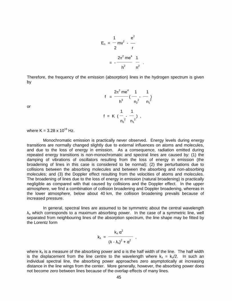
45
1 e
2
En =
mv2 -
2 r
22 me
4 1
= -
. h
2 n
2
Therefore, the frequency of the emission (absorption) lines in the hydrogen spectrum is given by
22 me
4 1 1
f =
(
-
) h
3 n2
2 n1
2
or 1 1
f = K (
-
) , n2
2 n1
2
where K = 3.28 x 10
15 Hz.
Monochromatic emission is practically never observed. Energy levels during energy
transitions are normally changed slightly due to external influences on atoms and molecules, and due to the loss of energy in emission. As a consequence, radiation emitted during repeated energy transitions is non-monochromatic and spectral lines are caused by: (1) the damping of vibrations of oscillators resulting from the loss of energy in emission (the broadening of lines in this case is considered to be normal); (2) the perturbations due to collisions between the absorbing molecules and between the absorbing and non-absorbing molecules; and (3) the Doppler effect resulting from the velocities of atoms and molecules. The broadening of lines due to the loss of energy in emission (natural broadening) is practically negligible as compared with that caused by collisions and the Doppler effect. In the upper atmosphere, we find a combination of collision broadening and Doppler broadening, whereas in the lower atmosphere, below about 40 km, the collision broadening prevails because of increased pressure.
In general, spectral lines are assumed to be symmetric about the central wavelength λo which corresponds to a maximum absorbing power. In the case of a symmetric line, well separated from neighbouring lines of the absorption spectrum, the line shape may be fitted by the Lorentz form
ko α2
kλ =
, (λ - λo)
2 + α
2
where kλ is a measure of the absorbing power and α is the half width of the line. The half width is the displacement from the line centre to the wavelength where kλ = ko/2. In such an individual spectral line, the absorbing power approaches zero asymptotically at increasing distance in the line wings from the center. More generally, however, the absorbing power does not become zero between lines because of the overlap effects of many lines.

46
3.6 Vibrational and Rotational Spectra
The Bohr theory of the hydrogen atom explained the quantized energy states available to an electron in orbit about a hydrogen nucleus. Additional consideration of elliptical orbits, relativistic effects, and magnetic spin orbit interaction was needed to explain the observed emission spectra in more detail (including the fine structure). Explanation of molecular emission lines requires still more work. Gaseous emission spectra are found to have atomic spectral lines with many additional molecular emission lines superimposed. As indicated earlier, three major types of molecular excitation are observed.
(a) The electronic excitation when the orbital states of the electrons change in individual atoms;
(b) The vibrational excitation when the individual atoms vibrate with respect to the combined molecular centre of mass;
(c) The rotational excitation when the molecule rotates about the centre of mass.
To illustrate the vibrational spectra, consider a typical potential energy curve for a diatomic molecule (shown in Figure 3.2). Stable equilibrium occurs with the nuclei separated by a distance Ro. If the nuclei are separated by a slightly greater or smaller distance R, the energy is raised and a spring-like restoring force results. This restoring force can be represented by
d2E
F = - ( _____
) (R - Ro) , dR
2
R=Ro
which has a classical frequency of vibration
1 d2E 1/2
fo =
(
) ,
2μ1/2
dR2 R=Ro
with the reduced mass of the vibrating system
M1 M2 μ =
.
M1 + M2 The energy levels can be shown to have the form of the Planck postulate
Em = (m + ½) hfo, m = 0, 1, 2, ... where the additional ½ is a consequence of solving the Schroedinger wave equation for a harmonic oscillator. The vibrational energy levels of a diatomic molecule are shown in Figure 3.2, the upper energy levels are not equally spaced since the actual energy well is wider than the parabolic approximation and hence these energy levels are closer together than the lower levels.

47
The rotational spectra appear as fine structure of the combined electronic and vibrational lines. The kinetic energy of rotation of the nuclei about their common centre of mass is readily solved with the Schroedinger equation and the following energy levels emerge:
h2
EJ =
J (J + 1), J = 1, 2, 3, ...
82μ Ro
2
These rotational energies are very small, and therefore, lines of the pure rotation spectrum are in the far infrared or microwave regions of the spectrum.
The total energy of a molecule is given by E = Eelectronic + Evibration + Erotation . The typical separation between the lowest state and the first excited state is about 2 to 10 eV for electronic energies, about .2 to 2 eV for vibration energies and about 10
-5 to 10
-3 eV for
rotation energies. Note that 1 eV = 1.6 x 10⁻¹⁹
J which corresponds to emission at a wavelength of 1.24 μm. Figure 3.3 illustrates this schematically.
Each transition involving a change in electron energy produces a whole series of emission or absorption lines, since many combinations of changes in vibration and rotation energy are possible. If such a system of lines is observed under low resolution conditions, it appears to be a band with practically a continuous distribution of frequencies. With higher resolution the individual lines can be resolved and the energy differences measured. In this way, the energies of the vibrational states and of the rotational states can be measured. It is apparent that in the higher vibrational states the average internuclear distance R is larger because of the asymmetry of the binding energy curve. This fact produces a higher moment of inertia μR
2 when the vibrational quantum number is large and a correspondingly smaller
separation in the rotational energy levels. Thus, precision measurement of the rotational levels as a function of vibrational quantum number permits the study of the asymmetry of the binding energy curve; it is this asymmetry that is responsible for the thermal expansion of molecules.
3.7 Summary of the Interactions between Radiation and Matter
One basic type of interaction between radiation and matter can be summarized by a photon transferring all of its energy to an atom or a molecule and thus being removed from the radiation field. The energy of the photon raises an electron to a higher energy level or a molecule to higher rotational or vibrational states. This increase in energy of the receiving atom or molecule can be released in several different ways.
One mechanism is for the activated molecule to collide with another molecule, and to drop back into a lower energy state; the energy thus freed becomes kinetic energy of the molecules and corresponds to warming the gas. This is absorption. The photon is permanently lost or attenuated from the radiation field.
A second mechanism for release of the energy increase is the spontaneous transition of the molecule (in about one nanosecond) into its original state by emitting a photon which is

48
identical to the absorbed one except for its direction of propagation. This is scattering, where the photon remains part of the radiation field but the direct beam is attenuated.
A third mechanism is the activated molecule releases its energy spontaneously but in two stages. Two photons with different lower energies result; the sum of the energies of the two photons equals the energy of the absorbed photon. The direct beam is attenuated; the original photon has been replaced by two photons at longer wavelengths and is no longer part of the radiation field. This is Raman-scattering.
Other mechanisms for energy release are fluorescence and phosphorescence. These occur when the energy is not released spontaneously, but after relaxation times of nanoseconds to hours.
Another basic type of interaction involves the conversion of molecular kinetic energy (thermal energy) into electromagnetic energy (photons). This occurs when molecules are activated by collisions with each other and the activation energy is emitted as photons. This is emission.
3.8 Beer's Law and Schwarzchild's Equation
In the absence of scattering, the absorption of parallel beam radiation as it passes downward through a horizontal layer of gas of infinitesimal thickness dz is proportional to the number of molecules per unit area that are absorbing radiation along the path. This relationship can be expressed in the form daλ = - dIλ / Iλ = - kλ ρ sec φ dz , where ρ is the density of the gas and φ is the zenith angle. Here absorbed monochromatic radiance is expressed as an incremental amount of depletion of the incident beam. dIλ and dz are both negative quantities, so daλ is positive. The product ρ sec φ dz is the mass within the volume swept out by a unit cross-sectional area of the incident beam as it passes through the layer, as pictured in Figure 3.4. The absorption coefficient kλ is a measure of the fraction of the gas molecules per unit wavelength interval that are absorbing radiation at the wavelength in question. kλ is a function of composition, temperature, and pressure of the gas within the layer. It has units of square metres per kilogram, which makes the product kλρ dz dimensionless. Integrating from z up to the top of the atmosphere yields
ln Iλ - ln Iλ = sec φ kλ ρ dz . z
Taking the anti-log of both sides and assuming kλ is independent of height,
Iλ = Iλ exp (- kλ u) ,
where

49
u = sec φ ρ dz . z
This relation, often referred to as Beer's Law, states that radiance decreases
monotonically with increasing path length through the layer. The quantity u is called the density weighted path length. kλu is a measure of the cumulative depletion that the beam of radiation has experienced as a result of its passage through the layer and is often called the optical depth σλ. The transmittance of the layer of gas lying above the level z is given by
-kλu
λ = Iλ / I λ = e and it follows that, in the absence of scattering, the absorptance
-kλu
aλ = 1 - λ = 1 - e approaches unity exponentially with increasing optical depth. At wavelengths close to the center of absorption lines, kλ is large so that a very short (density weighted) path length is sufficient to absorb virtually all the incident radiation. At wavelengths away from absorption lines, a path length many orders of magnitude longer may be required to produce any noticeable absorption.
Indirect calculation of the spectrum of solar radiation incident on the top of the atmosphere, on the basis of ground-based measurements, provides an interesting example of the application of Beer's law. Such calculations were made quite successfully many years before direct measurements of undepleted solar radiation were available from satellites. Writing Beer's Law in another form, we have
ln Iλ = ln Iλ - sec φ kλ ρ dz . z
Over the course of a single day, Iλ is measured at frequent intervals at a ground station. During this period, the numerical value of the integrand changes very little in comparison to the large changes in solar zenith angle. Thus, to a good approximation, the above expression assumes the form
ln Iλ = A – B x , where x = sec φ and A and B are constants; that is to say, when the individual data points for Iλ are plotted on a logarithmic scale as function of sec φ, they tend to fall along a straight line. Since the path length is directly proportional to x, it is possible to deduce the radiance upon the top of the atmosphere simply by extending the straight line that makes the best fit to the data points back to x = 0 (that is, zero path length through the atmosphere).
At the wavelengths of solar radiation, atmospheric emission is negligible, and only absorption needs to be considered. However, at the wavelengths of terrestrial radiation,

50
absorption and emission are equally important and must be considered simultaneously. The absorption of terrestrial radiation along an upward path through the atmosphere is described with the sign reversed by the relation
-dLλabs
= Lλ kλ ρ sec φ dz .
The emission of radiation from a gas can be treated in much the same manner as the absorption. Making use of Kirchhoff's law it is possible to write an analogous expression for the emission,
dLλem
= Bλ dλ = Bλ daλ = Bλ kλ ρ sec φ dz , where Bλ is the blackbody monochromatic radiance specified by Planck's law. Now we subtract the absorption from the emission to obtain the net contribution of the layer to the monochromatic radiance of the radiation passing upward through it: dLλ = - (Lλ - Bλ) kλ ρ sec φ dz . This expression, known as Schwarzchild's equation, is the basis for computations of the transfer of infrared radiation. For an isothermal gas, with constant kλ, this may be integrated to obtain (Lλ - Bλ) = (Lλo - Bλ) exp (- kλu) , where Lλo is the radiance incident on the layer from below. This expression shows that Lλ should exponentially approach Bλ as the optical thickness of the layer increases. For a layer of infinite optical thickness the emission from the top is Bλ regardless of the value of Lλo; that is to say, such a layer behaves as a blackbody.
It is often useful to transform the height variable z to pressure p through the
hydrostatic equation and the definition of mixing ratio q = ρ/ρa where ρ and ρa are the density of gas and air respectively,
g ρ dz = - q dp .
Thus, the optical depth becomes
p
u(p) = sec φ q g-1 dp ,
o and the monochromatic transmittance (the probability that a photon of wavelength l leaving pressure level p will reach the top of the atmosphere) is given by
p
λ(p) = exp [ - sec φ kλ g-1 q dp ] .
o

51
3.9 Atmospheric Scattering
Scattering is a physical process by which a particle in the path of an electromagnetic wave continuously abstracts energy from the incident wave and re-radiates that energy in all directions. Therefore, the particle may be thought of as a point source of the scattered energy. In the atmosphere, the particles responsible for scattering cover the sizes from gas molecules (~10
-8 cm) to large raindrops and hail particles (~1 cm). The relative intensity of the scattering
pattern depends strongly on the ratio of particle size to wavelength of the incident wave. If scattering is isotropic, the scattering pattern is symmetric about the direction of the incident wave. A small anisotropic particle tends to scatter light equally into the forward and backward directions. When the particle becomes larger, the scattered energy is increasingly concentrated in the forward directions. Distribution of the scattered energy involving spherical and certain symmetrical particles may be quantitatively determined by means of the electromagnetic wave theory. When particles are much smaller than the incident wavelength, the scattering is called Rayleigh scattering. For particles whose sizes are comparable to or larger than the wavelength, the scattering is customarily referred to as Mie scattering.
Rayleigh scattering indicates that the intensity scattered by air molecules in a specific direction is inversely proportional to the fourth power of the wavelength. A large portion of solar energy, lying between the blue to red portion of the visible spectrum, is Rayleigh scattered by
the atmosphere. Blue light ( 0.425 μm) has a shorter wavelength than red light ( 0.650 μm). Consequently, blue light scatters about 5.5 times more than red light. It is apparent that
the -4 law causes more of the blue light to be scattered than the red, the green, and the yellow,
and so the sky, when viewed away from the sun's disk, appears blue. Moreover, since the molecular density decreases drastically with height, it is anticipated that the sky should gradually darken to become completely black in outer space in directions away from the sun. And the sun itself should appear whiter and brighter with increasing height. As the sun approaches the horizon (at sunset or sunrise), sunlight travels through more air molecules, and therefore more and more blue light and light with shorter wavelengths are scattered out of the beam of light, and the luminous sun shows a deeper red colour than at the zenith.
Larger particles in the atmosphere such as aerosols, cloud droplets, and ice crystals also scatter sunlight and produce many fascinating optical phenomena. However, their single scattering properties depend less on wavelength and more upon the particle size. As a result of this, clouds in the atmosphere generally appear white instead of blue. In a cloudy atmosphere, the sky appears blue diluted with white scattered light, resulting in a less pure blue sky than would have been expected just from Rayleigh scattering. Scattering by a spherical particle of arbitrary size has been treated exactly by Mie in 1908 by means of solving the electromagnetic wave equation derived from the fundamental Maxwell equations.
It is possible to formulate an expression analogous to absorption for dsλ, the fraction of parallel beam radiation that is scattered when passing downward through a layer of infinitesimal thickness, namely dsλ = dIλ / Iλ = K A sec φ dz , where K is a dimensionless coefficient and A is the cross-sectional area that the particles in a unit volume present to the beam of incident radiation. If all the particles that the beam encounters in its passage through the differential layer were projected onto a plane perpendicular to the incident beam, the product A sec φ dz would represent the fractional area

52
occupied by the particles. Thus, K plays the role of a scattering area coefficient which measures the ratio of the effective scattering cross section of the particles to their geometric cross section. In the idealized case of scattering by spherical particles of uniform radius r, the scattering area coefficient K can be prescribed on the basis of theory. It is convenient to express K as a function of a dimensionless size parameter α = 2πr/λ, which is a measure of the
size of the particles in comparison to the wavelength of the incident radiation. Figure 3.5a shows a plot of α as a function of r and λ. The scattering area coefficient K depends not only upon the size parameter, but also upon the index of refraction of the particles responsible for the scattering. Figure 3.5b shows K as a function of α for two widely differing refractive indices. When α << 1 we have Rayleigh scattering (K~α
4), and between 0.1 and 50 we are in the Mie
regime. For α>50 the angular distribution of scattered radiation can be described by the principles of geometric optics. The scattering of visible radiation by cloud droplets, raindrops, and ice particles falls within this regime and produces a number of distinctive optical phenomena such as rainbows and halos.
It should be noted that for terrestrial radiation, scattering in the atmosphere is of secondary importance compared to absorption and emission.
3.10 The Solar Spectrum
The solar spectrum refers to the distribution of electromagnetic radiation emitted by the sun as a function of the wavelength incident on the top of the atmosphere. The solar constant S is a quantity denoting the amount of total solar irradiance reaching the top of the atmosphere. We recall that it is defined as the flux of solar energy (energy per time) across a surface of unit area normal to the solar beam at the mean distance between the sun and earth. The solar spectrum and solar constant have been extensively investigated for some time. Abbot undertook a long series of ground-based measurements, resulting in a value of about 1350 Wm
-2 for the solar constant. Subsequent to Abbot's work and prior to more recent
measurements carried out from high-altitude platforms, solar constant values of 1396 and 1380 Wm
-2, proposed by Johnson and Nicolet respectively, were widely accepted. Since July 1985,
the Earth Radiation Budget Experiment (ERBE) has been monitoring the sun's radiation . The solar constant measurements from Nimbus 7 indicate a value of 1372 Wm
-2 with generally less
than a 0.1% variation. There are some significant short term fluctuations due to decreases associated with the development of sunspots.
The standard solar spectrum in terms of the spectral irradiance is shown in the top solid curve of Figure 3.6. Also shown in this diagram is the spectral solar irradiance reaching sea level in a clear atmosphere. The shaded areas represent the amount of absorption by various gases in the atmosphere, primarily H2O, CO2, O3, and O2. Absorption and scattering of solar radiation in clear atmospheres will be discussed later. If one matches the solar spectral irradiance curve with theoretical blackbody values, we find that a temperature around 6000 K fits the observed curve closely in the visible and infrared wavelengths. Most of the electromagnetic energy reaching the earth originates from the sun's surface, called the photosphere. Of the electromagnetic energy emitted from the sun, approximately 50% lies in wavelengths longer than the visible region, about 40% in the visible region (0.4-0.7 μm), and about 10% in wavelengths shorter than the visible region.

53
3.11 Composition of the Earth's Atmosphere
To describe the interaction of the earth's atmosphere with solar radiation, the atmosphere's composition must be understood. The atmosphere is composed of a group of nearly permanent gases and a group of gases with variable concentration. In addition, the atmosphere also contains various solid and liquid particles such as aerosols, water drops, and ice crystals, which are highly variable in space and time.
Table 3.2 lists the chemical formula and volume ratio for the concentrations of the permanent and variable gases in the earth's atmosphere. It is apparent from this table that nitrogen, oxygen, and argon account for more than 99.99% of the permanent gases. These gases have virtually constant volume ratios up to an altitude of about 60 km in the atmosphere. It should be noted that although carbon dioxide is listed here as a permanent constituent, it's concentration varies as a result of the combustion of fossil fuels, absorption and release by the ocean, and photosynthesis. Water vapour concentration varies greatly both in space and time depending upon the atmospheric condition. Its variation is extremely important in the radiative absorption and emission processes. Ozone concentration also changes with respect to time and space, and it occurs principally at altitudes from about 15 to about 30 km, where it is both produced and destroyed by photochemical reactions. Most of the ultraviolet radiation is absorbed by ozone, preventing this harmful radiation from reaching the earth's surface.
3.12 Atmospheric Absorption and Emission of Solar Radiation The absorption and emission of solar radiation in the atmosphere is accomplished by molecular storing of the electromagnetic radiation energy. Molecules can store energy in various ways. Any moving particle has kinetic energy as a result of its motion in space. This is known as translational energy. The averaged translational kinetic energy of a single molecule in the x, y and z directions is found to be equal to kT/2, where k is the Boltzmann constant and T is the absolute temperature. A molecule which is composed of atoms can rotate, or revolve, about an axis through its centre of gravity and, therefore, has rotational energy. The atoms of the molecule are bounded by certain forces in which the individual atoms can vibrate about their equilibrium positions relative to one another. The molecule, therefore, will have vibrational energy. These three molecular energy types (translational, rotational, and vibrational) are based on a rather mechanical model of the molecule that ignores the detailed structure of the molecule in terms of nuclei and electrons. It is possible, however, for the energy of a molecule to change due to a change in the energy state of the electrons of which it is composed. Thus, the molecule also has electronic energy. The energy levels are quantized and take discrete values only. As we have pointed out, absorption and emission of radiation takes place when the atoms or molecules undergo transitions from one energy state to another. In general, these transitions are governed by selection rules. Atoms exhibit line spectra associated with electronic energy levels. Molecules, however, also have rotational and vibrational energy levels that lead to complex band systems.
Solar radiation is mainly absorbed in the atmosphere by O2, O3, N2, CO2, H2O, O, and N, although NO, N2O, CO, and CH4, which occur in very small quantities, also exhibit absorption spectra. Absorption spectra due to electronic transitions of molecular and atomic oxygen and nitrogen, and ozone occur chiefly in the ultraviolet (UV) region, while those due to the vibrational and rotational transitions of triatomic molecules such as H2O, O3, and CO2 lie in the infrared region. There is very little absorption in the visible region of the solar spectrum.

54
3.13 Atmospheric Absorption and Emission of Thermal Radiation
The earth also emits electromagnetic radiation covering all frequencies. However, the global mean temperature of the earth-atmosphere system is only about 250 K, a temperature that is obviously much lower than that of the sun's photosphere. As a consequence of Planck's law and Wien's displacement law discussed earlier, the radiance (intensity) peak of the Planck function is smaller for the earth's radiation field and the wavelength for the radiance (intensity) peak of the earth's radiation field is longer. The energy emitted from the earth-atmosphere system is called thermal infrared (or terrestrial) radiation. Figure 1.1 showed the earth radiance to space measured by the Infrared Interferometer Spectrometer Instrument (IRIS) on board Nimbus IV as well as the spectral distribution of radiance emitted by a blackbody source at various temperatures in the terrestrial range (in terms of wavenumber). In some spectral regions the envelope of the emission spectrum is very close to the spectrum emitted from a blackbody with a temperature of about 300 K, which is about the temperature of the surface. In these spectral regions, the atmosphere is transparent to that radiation. In other spectral regions the emission spectrum is close to the spectrum emitted from a blackbody with a temperature of about 220 K, which is about the temperature at the tropopause. This occurs in spectral regions where the atmosphere is opaque or absorbing to that radiation and the atmosphere is said to be trapping the radiation.
Figure 3.7 shows more recent measurements from an airborne interferometer; clearly,
in certain portions of the infrared spectrum, radiation is trapped by various gases in the atmosphere. Among these gases, carbon dioxide (CO2), water vapour (H2O), and ozone (O3) are the most important absorbers. Some minor constituents (which are not shown in Figure 3.7), such as carbon monoxide (CO), nitrous oxide (N2O), methane (CH4), and nitric oxide (NO) are relatively insignificant absorbers insofar as the heat budget of the earth-atmosphere is concerned. CO2 absorbs infrared radiation significantly in the 15 μm band (in the wavenumber domain from about 600 to 800 cm
-1, which also corresponds to the maximum intensity of the
Planck function). H2O absorbs thermal infrared in the 6.3 μm band (from about 1200 to 2000 cm
-1) and in the rotational band beyond 20 μm (< 500 cm
-1). Except for O3, which has an
absorption band in the 9.6 μm region (about 1040 cm-1), the atmosphere is relatively
transparent from 8 to 12 μm (800 to 1200 cm-1). This region is referred to as the atmospheric
window. CO2 also has an absorption band in the shorter wavelength of the 4.3 μm region (2325 cm
-1). The global distribution of CO2 is fairly uniform, although there has been
observational evidence indicating a continuous global increase over the past century owing to increased combustion of fossil fuels. This leads to the question of the earth's climate and possible climatic changes due to the increasing CO2 concentration. Unlike CO2, however, H2O and O3 are highly variable both with respect to time and the geographical location. These variations are vital to the radiation budget of the earth-atmosphere system and to long-term climatic changes.
Figure 3.8 shows the radiance from 0.1 μm to 10 cm emitted by the earth-atmosphere system transmitted to space. In a clear atmosphere without clouds and aerosols, a large portion (about 50%) of solar energy transmits through the atmosphere and is absorbed by the earth's surface. Energy emitted from the earth, on the contrary, is absorbed largely by carbon dioxide, water vapour, and ozone in the atmosphere as evident in Figure 3.7. Trapping of thermal infrared radiation by atmospheric gases is typical of the atmosphere and is, therefore, called the atmospheric effect.

55
Solar radiation is referred to as shortwave radiation because solar energy is concentrated in shorter wavelengths with its peak at about 0.5 μm. Thermal infrared radiation from the earth's atmosphere is referred to as longwave radiation because its maximum energy is in the longer wavelength at about 10 μm. The solar and infrared spectra are separated into two spectral ranges above and below about 4 μm, and the overlap between them is relatively insignificant. This distinction makes it possible to treat the two types of radiative transfer and source functions separately and thereby simplify the complexity of the transfer problem.
3.14 Atmospheric Absorption Bands in the Infrared Spectrum
Inspection of high resolution spectroscopic data reveals that there are thousands of absorption lines within each absorption band. The fine structure of molecular absorption bands for the 320-380 cm
-1 is due to water vapour, and for the 680-740 cm
-1 region it is due to carbon
dioxide. The optically active gases of the atmosphere, carbon dioxide, water vapour, and ozone are all triatomic molecules. Figure 3.9 shows the absorption spectra for H2O and CO2. Spectroscopic evidence indicates that the three atoms of CO2 form a symmetrical straight line array having the carbon atom in the middle flanked by oxygen atoms in either side. Because of linear symmetry it cannot have a static electric dipole moment. Figure 3.10a shows the three normal modes of vibration of such a configuration. The symmetrical motion v1 should not give rise to an electric dipole moment and, therefore, should not be optically active. The v1 vibration mode has been identified in the Raman spectrum near 7.5 μm. In the v2 vibration mode, the dipole moment is perpendicular to the axis of the molecule. The 15 μm band represents this particular vibration. The band is referred to as a fundamental because it is caused by a transition from the ground state to the first excited vibrational state. Another fundamental corresponding to the v3 vibration mode is the 4.3 μm band, which appears at the short-wave edge of the blackbody curve of atmospheric temperatures.
The water molecule forms an isosceles triangle which is obtuse. Figure 3.10b shows the three normal modes of vibration for such a structure. The 6.3 μm band has been identified as the v2 fundamental. The two fundamentals, v1 and v3, are found close together in a band near 2.7 μm, i.e., on the shortwave side of the infrared spectral region.
The band covering the region from 800 to 400 cm-1 shown in Figure 3.7 represents the
purely rotational spectrum of water vapour. The water molecule forms an asymmetrical top with respect to rotation, and the line structure of the spectrum does not have the simplicity of a symmetrical rotator such as found in the CO2 molecule. Close inspection shows that the absorption lines have no clear-cut regularity. The fine structure of the 6.3 μm band is essentially similar to that of the pure rotational band.
In the region between about 8 and 12 μm, the so-called atmospheric window, absorption is continuous and is primarily due to water vapour. Absorption by carbon dioxide is typically a small part of the total in this region. The overlap of water vapour with ozone in this region is insignificant in the computations of cooling rates since water vapour is important mainly in the lower atmosphere, while cooling due to ozone takes place primarily in the stratosphere and higher.
The ozone molecule is of the triatomic nonlinear type (Figure 3.10b) with a relatively strong rotation spectrum. The three fundamental vibrational bands v1, v2, and v3 occur at wavelengths of 9.066, 14.27, and 9.597 μm, respectively. The very strong v3 and moderately

56
strong v1 fundamentals combine to make the well-known 9.6 μm band of ozone. The v2 fundamental is well-masked by the 15 μm band of CO2. The strong band of about 4.7 μm produced by the overtone and combination frequencies of 03 vibrations is in a weak portion of the Planck energy distribution for the atmosphere. Note that the absorption bands of O3 in the UV part of the solar spectrum are due to electronic transitions in the ozone molecule.
3.15 Atmospheric Absorption Bands in the Microwave Spectrum
While most of the focus of this chapter has been the visible and infrared spectral regions, a brief summary of the absorption lines in the microwave spectral region follows. Molecular oxygen and water vapour are the major absorbing constituents here. Figure 3.11 shows the transmittance for frequencies below 300 GHz. Below 40 GHz only the weakly absorbing pressure broadened 22.235 GHz water vapour line is evident; this line is caused by transitions between the rotational states. At about 60 and 118.75 GHz, there are strong oxygen absorption lines due to magnetic dipole transitions. For frequencies greater than 120 GHz, water vapour absorption again becomes dominant due to the strongly absorbing line at 183 GHz.
A special problem in the use of microwave from a satellite platform is the emissivity of the earth surface. In the microwave region of the spectrum, emissivity values of the earth surface range from .4 to 1.0. This complicates interpretation of terrestrial and atmospheric radiation with earth surface reflections. More will be said about this later.
3.16 Remote Sensing Regions
Several spectral regions are considered useful for remote sensing from satellites. Figure 3.12 summarizes this. Windows through the atmosphere (regions of minimal atmospheric absorption) exist near 4 μm, 10 μm, 0.3 cm, and 1 cm. Infrared windows are used for sensing the temperature of the earth surface and clouds, while microwave windows help to investigate the surface emissivity and the liquid water content of clouds. The CO2 absorption bands at 4.3 and 15 μm and the O2 bands at 0.25 and 0.5 cm are used for temperature profile retrieval; because these gases are uniformly mixed in the atmosphere in known portions they lend themselves to this application. The water vapour absorption bands near 6.3 μm, beyond 18 μm, near 0.2 cm, and near 1.3 cm are sensitive to the water vapour concentration in the atmosphere.
In summary, incoming solar radiation (mostly visible) drives the earth-atmosphere
(which emits infrared). The atmosphere transmits, absorbs (by H2O, O2, O3, dust), reflects (by clouds), and scatters (by aerosols) incoming visible; the earth surface absorbs and reflects the transmitted visible. Atmospheric H2O, CO2, and O3 selectively transmit or absorb the outgoing infrared radiation. The outgoing microwave is primarily affected by H2O and O2. The atmosphere has window regions where radiation is mostly transmitted (but some absorption occurs in all parts of the spectrum). The earth surface emits with efficiency less than blackbody at all wavelengths (but in the infrared window regions the emissivity is close to one for some surfaces). Figure 13.3 summarizes the infrared atmospheric absorptance and selected earth surface emissivities.

57
Table 3.1: Reflectance (in percent) of various surfaces in the spectral range of solar radiation (using the US Standard Atmosphere of 1976)
Bare soil
10 - 25
Sand, desert
25 - 40
Grass
15 - 25
Forest
10 - 20
Snow (clean, dry)
75 - 95
Snow (wet, dirty)
25 - 75
Sea surface (sun angle > 25)
< 10
Sea surface (low sun angle)
10 - 70

58
Table 3.2: Composition of the Atmosphere (from the US Standard Atmosphere of 1976)
Permanent Constituents Variable Constituents
% by Volume % by Volume
_________________________________________________________________________ Nitrogen (N2) 78.084 Water vapour (H2O) 0-0.04 Oxygen (O2) 20.948 Ozone (O3) 0-12x10
-4
Argon (Ar) 0.934 Sulfur dioxide (SO2)
1 0.001x10
-4
Carbon dioxide (CO2) 0.033 Nitrogen dioxide (NO2)
1 0.001x10
-4
Neon (Ne) 18.18x10
-4 Ammonia (NH3)
1 0.004x10
-4
Helium (He) 5.24x10
-4 Nitric oxide (NO)
1 0.0005x10
-4
Krypton (Kr) 1.14x10
-4 Hydrogen sulfide (H2S) 10.00005x10
-4
Xenon (Xe) 0.089x10⁻⁴
Nitric acid (HNO3) Trace Hydrogen (H2) 0.5x10
-4
Methane (CH4) 1.5x10⁻⁴
Nitrous oxide (N2O)1 0.27x10
-4
Carbon monoxide (CO)1 0.19x10
-4
_________________________________________________________________________
1
Concentration near the earth's surface.

59
Figure 3.1: Schematic for reflectance, absorptance, and transmittance in a layer of gases.
Figure 3.2: Vibrational energy levels of a diatomic molecule.

60
Figure 3.3: Energy levels of a diatomic molecule. Every level of electronic + vibrational energy has rotational fine structure, but this structure is illustrated only for the n = 2 states.
Figure 3.4: Depletion of an incident beam of unit cross-section while passing through an absorbing layer of infinitesimal thickness.

61
Figure 3.5a: Size parameter a as a function of incident radiation and particle radius.
Figure 3.5b: Scattering area coefficient K as a function of size parameter for refractive indices of 1.330 (solid curve) and 14.86 (dashed curve).

62
Figure 3.6: Spectral irradiance distribution curves related to the sun: (1) the observed solar irradiance at the top of the atmosphere (after Thekaekara, 1976); and (2) solar irradiance observed at sea level. The shaded areas represent absorption due to various gases in a clear atmosphere.
Earth emitted spectra overlaid on Planck function envelopes
CO2
H20
O3
CO2
Figure 3.7: Earth-atmosphere emitted radiances overlaid on Planck function envelopes.

63
Figure 3.8a: Atmospheric transmission characteristics showing the major absorption bands.
Spectral Characteristics of
Atmospheric Transmission and Sensing Systems
Figure 3.8b: Atmospheric transmission characteristics and the associated remote sensing technologies.

64
Figure 3.9: Absorption spectrum of the water vapour rotational band (beyond 18 μm) and the carbon dioxide band (near 15 μm) at high spectral resolution.
Figure 3.10: Normal modes of linear (a) and triangular (b) molecules.

65
Figure 3.11: Atmospheric transmittance in the microwave region of the spectrum as a function of frequency.
Figure 3.12: Spectral regions used for remote sensing of the earth atmosphere and surface
from satellites. indicates emissivity, q denotes water vapour, and T represents temperature.

66
Figure 3.13: Infrared atmospheric absorption (top) and earth surface emissivity for some surfaces (bottom).

67
CHAPTER 4
THE RADIATION BUDGET
4.1 The Mean Global Energy Balance
Figure 4.1 summarizes the annual mean global energy balance for the earth-atmosphere system and indicates some of the atmospheric processes that come into play. Of the 100 units of incident solar radiation, 19 are absorbed during passage through the atmosphere: 16 in cloud-free air and three in clouds. A total of 30 units are reflected back to space: 20 from clouds, six from cloud-free air, and four from the earth’s surface. The remaining 51 units are absorbed at the earth’s surface. The earth disposes of this energy by a combination of infrared radiation and sensible and latent heat flux. The net infrared emission, which represents the upward emission from the earth’s surface, minus the downward emission from the atmosphere, amounts to 21 units, 15 of which are absorbed in passing through the atmosphere and six of which reach space. The remaining 30 units are transferred from the earth’s surface to the atmosphere by a combination of latent and sensible heat flux.
From the viewpoint of the atmosphere alone, there is a net loss of 49 units of infrared radiation (70 units emitted to space from the top of the atmosphere minus 21 units of net upward flux from the earth’s surface) which exceeds by 30 units, the energy gained as a result of the absorption of solar radiation. This deficit is balanced by an influx of 30 units of latent and sensible heat from the earth’s surface. Thus, in the global average, the atmosphere experiences a net radiative cooling which is balanced by the latent heat of condensation that is released in regions of precipitation, and by the conduction of sensible heat from the underlying surface. Were it not for the fluxes of latent and sensible heat, the earth’s surface would have to be considerably hotter (on the order of 340 K as compared with the observed value of 288 K) in order to emit enough infrared radiation to satisfy the balance requirements for thermal equilibrium.
4.2 The First Satellite Experiment to Measure the Net Radiation
The radiation budget of net radiation, N, of the entire earth-atmosphere system is the difference between the absorbed solar radiation and the outgoing longwave radiation, N = (1 - A) S/4 - RLW, where A is the fraction of incoming solar energy reflected back to space (the planetary albedo), S is the incoming solar irradiance, and RLW is the outgoing longwave irradiance. The radiation budget equation can be written for a specific location of the earth at a given instant of time by replacing the planetary mean incoming solar radiation term ( S/4 ) with the term S cos φ, where φ is the solar zenith angle at the location and time of interest. In this case, A is no longer the planetary albedo, but instead the bi-directional reflectance of the earth-atmosphere for that specific location and time.
The first meteorological satellite experiment flew on the Explorer VII satellite in 1959. The experiment was devised by Suomi and Parent to provide this most basic meteorological

68
measurement, the balance between the radiation input to the atmosphere from the sun and the radiation exiting from the atmosphere as a result of reflection and emission processes. The spatial distribution of the radiation imbalances between incoming and outgoing radiation (the net radiation) is the primary driving force of atmospheric circulation. The solar input had already been measured from ground-based and balloon borne platforms. Suomi’s experiment was the first to measure the energy loss to space.
Suomi’s radiometer (or more correctly bolometer) consisted of two heat sensing
detectors, one painted black to absorb radiation at all wavelengths, and the other painted white to reflect the sun’s energy and thereby absorbed only earth emitted radiation. Thus, Suomi was able to differentiate between the energy leaving the earth’s atmosphere due to reflected sunlight (provided by the difference between radiation sensed by the black and white sensors) and that emitted by the earth and atmosphere (radiation measured by the white sensor).
In a short time after exposure to various radiative components involving the direct solar flux, solar flux reflected by the earth and atmosphere (shortwave), and thermal infrared flux emitted by the earth and atmosphere (longwave), each sensor achieves radiative equilibrium. It is assumed that the absorptivity of the black sensor ab is the same for shortwave and longwave radiation. However, the absorptivity of the white sensor for shortwave and longwave radiation are given by aw
S and aw
L, respectively. Let the temperatures measured by the black
sensors and white sensors be Tb and Tw, respectively. On the basis of the Stefan-Boltzmann and Kirchhoff laws, radiative equilibrium equations for both sensors may be expressed by
4r2 ab σTb
4 = r
2 ab (Eo +ES + EIR)
and
4r2 aw
L σTw
4 = r
2 [aw
S (Eo + Es) + aw
L EIR] .
These two equations show that the emitted energy per unit time is equal to the
absorbed energy per unit time, where 4r2 and r
2 represent the emission and absorption
areas, respectively, for the two spherical sensors each with a radius r. The irradiances of the reflected shortwave, longwave radiation, and direct solar are denoted by ES, EIR, and EO, respectively.
Upon solving the sum of the shortwave and the longwave irradiances, we obtain Eo + ES = [4 σ aw
L / (aw
L - aw
S) ] (Tb
4 - Tw
4)
and
EIR = [4 σ /( awL - aw
S) ] (aw
L Tw
4 - aw
S Tb
4)
The direct solar irradiance EO can be evaluated from the solar constant, which is specified prior to the experiment.
In order to convert the measured irradiances into radiances emitted and reflected by the earth, one must consider the solid angle Ω which the earth subtends to the satellite sensor. For a satellite at height h above the earth surface, it can be shown from simple geometric considerations that
Ω = 2 [ 1 - (2Rh + h2)½ / (R + h) ],

69
where R represents the radius of the earth. Then the radiance I is given by I = E/Ω , since the spherical sensor is equally sensitive to radiation from all directions, eliminating the cosine dependence with respect to angle of incidence.
4.3 The Radiation Budget
The circulation of the earth’s atmosphere and oceans can be thought of as being powered by a heat engine. The shortwave radiation from the sun provides the fuel supply while the infrared radiation heat loss to space from the earth’s surface and atmosphere is the exhaust. The engine is throttled, to a large extent, by storms and ocean disturbances associated with the transformation of radiative heat to latent and sensible heat.
The distribution of sunlight with latitude is responsible for our major climatic zones
(Tropical, Temperate, and Polar). The composition of the atmosphere and the characteristics of the earth’s surface also play an important role in the climate of local regions such as deserts. Small changes in the sun’s radiation or the terrestrial radiation due to natural or man induced changes in atmosphere and surface composition might lead to major variations in our climate.
The net radiation for the earth may vary through the year in accordance with earth-sun
distance since S varies 6% between January and July. However, when integrated over an entire year, the net radiation must be near zero, otherwise long-term climatic changes would occur. On the planetary and regional scales, clouds play the major role in upsetting the normal state of radiation balance. The importance of clouds in the radiation balance is demonstrated in Figure 4.2. It shows the relation between the longwave radiation to space as a function of cloud amount and height for standard atmospheric temperature and moisture conditions. Also shown is the absorbed solar radiation as a function of cloud amount. The longwave radiation to space decreases with increasing cloud cover and cloud height because cloud temperatures are considerably lower than the earth’s surface and they decrease with cloud elevation. However, clouds are also good reflectors of solar radiation so that the global albedo increases with increasing cloud cover since clouds generally have higher albedos than the earth’s surface. And as a consequence the absorbed solar energy decreases.
Figure 4.3a displays the globally averaged monthly mean values of various radiation budget parameters from July 1975 through December 1976. The annual cycles seem to repeat, as the values observed during July 1976 through December 1976 are nearly the same as those observed one year earlier. The albedo and longwave radiation cycles are nearly six months out of phase, possibly the result of two phenomena - the variation of the longwave radiation with time and the annual cycle of cloudiness. With regard to longwave radiation, in the Northern Hemisphere, the heating and cooling rates correspond to that expected for land surfaces, so outgoing longwave radiation reaches a maximum in July and a minimum in December. In the Southern Hemisphere, it is dominated by sea surfaces, so only a weak cycle is observed because the seasonal variation of sea-surface temperature is negligible. Therefore, the variation of the globally averaged longwave radiation with time is dominated by the Northern Hemisphere. During the months when the longwave radiation is at a minimum, the snow and ice cover and thus albedo in the Northern Hemisphere are close to a maximum.

70
When the longwave radiation is at a maximum, the snow and ice cover are greatly reduced. With regard to the equally important annual cycle of cloudiness, there tends to be more cloudiness in the Northern Hemisphere winter than in the Southern Hemisphere winter. This increases the albedo and decreases the longwave radiation. The opposite effect occurs around June when the cloudiness is least.
As shown in Figure 4.3b, the variation with time in the absorbed solar radiation (incoming minus reflected solar radiation) appears to be principally dependent upon the variation of the incoming solar radiation. The annual variation of the incoming solar radiation about its mean value is ±11.4 W m
-2, while the variation of the net energy about its mean value
is only about ±7.6 W m-2; the two are nearly in phase with each other. If the earth were in a
perfectly circular orbit around the sun so that there were no variations in the incoming radiation due to variations in the earth-sun distance, then the variation in absorbed solar radiation would be dominated by variation in the reflected energy. This would cause the phase of the absorbed solar radiation to be shifted about six months from that observed. Minima and maxima of the absorbed solar radiation correspond to maxima and minima, respectively, of the reflected radiation. Since the net radiation is the difference of the absorbed solar radiation and the outgoing longwave radiation, which are nearly six months out of phase with each other, the variation in the net radiation has an amplitude exceeding that of the absorbed and outgoing components and nearly the same phase as the absorbed solar radiation.
4.4 Distribution of Solar Energy Intercepted by the Earth
The solar irradiance at the top of the atmosphere depends strongly on the zenith angle of the sun and much less strongly on the variable distance of the earth from the sun. If the zenith angle, θ, is assumed to be constant over the solid angle subtended by the sun, the irradiance on a horizontal surface varies as cos θ. The zenith angle depends on latitude, time of day, and the tilt of the earth’s axis to the rays of the sun (celestial longitude). The mean value of the earth-sun distance, Res
m, is about 1.495 x 10
11 meters. The minimum distance
occurs on about 3 January during perihelion and is 1.47 x 10¹¹
meters; the maximum distance occurs on about 5 July during aphelion and is 1.52 x 10
11 meters.
The total energy received per unit area per day, called insolation and denoted by QO,
can be calculated by integrating over the daylight hours as follows:
sunset
Qo = S (Resm / Res)
2 cos θ dt
sunrise where S represents the mean solar irradiance.
Figure 4.4 shows the results of evaluating QO for a variety of latitudes and dates. The maximum insolation occurs at summer solstice at either pole. This is the result of the 24 hour solar day. The maximum in the Southern Hemisphere is higher than in the Northern Hemisphere because the earth is closer to the sun during the northern winter than during the northern summer.

71
4.5 Solar Heating Rates
Absorption of solar radiation by various gases results in heating in the atmosphere. Heating rate variation with atmospheric pressure is derived from net flux considerations. Starting with a plane parallel absorbing and scattering atmosphere, let the differential thickness within the atmosphere be dz and the monochromatic downward and upward irradiances at
wavelength λ be Eλ and Eλ
respectively. The net monochromatic irradiance (downward) at a given altitude is then given by
Eλ (z) = Eλ (z) - Eλ
(z) . Because of absorption, the net monochromatic irradiance decreases from the upper levels to the lower levels. The loss of net monochromatic irradiance or the divergence for the differential layer is given by dEλ (z) = Eλ (z) - Eλ (z + dz) From the definition of absorption, we also have
dEλ (z) = - Eλ (z + dz) aλ (dz)
Energy conservation requires that the absorbed energy has to be used to heat the layer, so that dEλ (z) = - ρ Cp dz dT / dt where ρ is the air density in the layer, Cp is the specific heat capacity at constant pressure, and t is the time. Combining these expressions yields the heating rate
dT/dt = Eλ (z + dz) aλ (dz) / (ρ Cp dz)
The heating rate is explicitly a function of spectral interval; to derive a total heating rate it is necessary to sum the spectral intervals where the absorption coefficient is non zero.
Figure 4.5 shows the solar heating rate profile up to 30 km using two different atmospheric profiles (mid latitude winter and tropical) for a clear atmosphere with the sun directly overhead. Effects of absorption by O3, H2O, O2, and CO2, multiple scattering by molecules, and the ground reflection are accounted for. The maximum heating rate is seen to occur at 3 km and have a value as high as 4 C per day. The heating rate decreases drastically with increasing altitude due to the decrease of water vapour concentration and reaches a minimum at roughly 15 km. Above 20 km, the increased solar heating is caused by the absorption of ozone, which has a maximum concentration at about 25 km.
4.6 Infrared Cooling Rates
Emission (absorption) of infrared radiation by various gases produces a cooling (heating) effect in the atmosphere. In the same way that solar heating is a function of the net transfer of radiation in the downward direction (as solar radiation enters from the top of the atmosphere), infrared cooling is a function of the net transfer of radiation in the upward

72
direction (as thermal radiation can be thought of as originating from the earth surface). An analogous derivation yields dT/dt = - (dEλ / dz) / (ρ Cp) where dEλ represents the net loss of irradiance in the layer dz.
A calculation of infrared cooling rates as a function of height in the clear tropical atmosphere is illustrated in Figure 4.6. In the lower 2 km the water vapour continuum influences the cooling due to the rapid increase in the temperature and the partial pressure of water vapour as one gets closer to the surface. Above 5 km the water vapour continuum contributes very little to the infrared cooling rate. In the middle and upper troposphere, absorption is mostly in the water vapour rotational band. A large increase in ozone concentration between 18 and 27 km results in a strong heating. Above 30 km the cooling rate
increases rapidly due to the CO2 15 m and O3 9.6 m absorption bands.
4.7 Radiative Equilibrium in a Gray Atmosphere
The concept of a balanced atmosphere that transfers energy only through radiative transfer (no conduction or convection) is useful for deriving some of the characteristics of the earth atmosphere. Given a heated surface and a gray atmosphere that is in balance, one can write that the net irradiance at any level is constant, since
d/dz [E - E] = ρ Cp dT/dt = 0 (1) The irradiance going up through a layer can be written
d/dχ* [E] = E - B (2) and similarly for the irradiance going down through a layer
-d/dχ* [E] = E - B (3) where πB is given by Stefan’s Law and χ* is an effective optical depth integrated from the top of the atmosphere down over all angles in the hemisphere. Adding equations (2) and (3) yields
d/dχ* [E - E] = E + E - 2B = 0 , (4)
and subtracting (2) - (3) gives
d/dχ* [E + E] = [E - E] = = const. (5)
or using (4)
B = χ* / 2 + Bo . (6) The boundary conditions are such that at the top of the atmosphere there is no downward irradiance

73
E(top) = 0 , and χ*(top) = 0 , and at the bottom of the atmosphere the upward irradiance must be dictated by Stefan’s Law applied to the surface temperature
E(bot) = σ T(sfc)4 , and
χ*(bot) = χ*(tot) where χ*(tot) is the effective optical depth of the total atmosphere. Then we find that
B = (χ*+1) / 2 , and (7)
[B(sfc) - B(bot)] = /2 . (8)
The function B is plotted against χ* in Figure 4.7. At the surface there is a discontinuity in temperature, as dictated by Eq. (8). Combining Eq. (7) and (8)
B(sfc) = (χ*(tot) +2) / 2 . (9) Or written more simply in terms of temperature T(sfc)
4 - T(top)
4 = T(bot)
4 (10)
and χ*(tot) = [T(sfc)
4 / T(top)
4] - 2 . (11)
When the atmosphere effective optical depth is large, the surface temperature is enhanced, as expected by the greenhouse effect. The optical depth of an atmosphere depends on the concentration of H2O, CO2, and O3. In the case of H2O the concentration may increase with increasing temperature (through evaporation) and thus create positive feedback for the greenhouse effect. This effect is very noticeable on Venus, which exhibits a “runaway greenhouse effect.”
Figure 4.8 shows the equivalent diagram in terms of temperature and height to Figure
4.7. The lower part of the atmosphere shows a very steep lapse rate of temperature that is unstable with respect to vertical motion; in a more realistic atmosphere, convection would tend to establish a mean adiabatic lapse rate. Air from near the surface would tend to rise along the mean adiabatic lapse rate of -6 K / km and intersect with the radiative equilibrium curve at a height of about 10 km or near the tropopause. In mid-latitudes the tropopause divides the troposphere where convection is dominant from the stratosphere where radiative transfer is dominant.

74
Figure 4.1: The annual mean global energy balance for the earth-atmosphere system. (Numbers are given as percentages of the globally averaged solar irradiance incidence upon the top of the atmosphere.)
Figure 4.2: Longwave radiation to space, R, and absorbed solar radiation, Q, as a function of cloud amount.

75
(a)
(b)
Figure 4.3: (a) Globally averaged monthly mean values of radiation budget parameters. (b) Variation in time with respect to an annual mean of net, incoming, and outgoing radiation.
Figure 4.4: Daily solar insolation in W/m2 incident on a horizontal surface at the top of the
atmosphere as a function of latitude and date (adapted from Milankovitch, 1930).

76
Figure 4.5: Solar heating rate calculated from atmospheric profiles appropriate for tropical and mid latitude winter conditions (Liou, 1980).
Figure 4.6: Calculation of total and partial cooling rates with an atmospheric profile appropriate for clear tropical conditions (after Roewe and Liou, 1978).

77
Figure 4.7: Upward E and downward E irradiance and emitted radiance from a given layer
B (given by Stefan’s Law) plotted as a function of effective optical depth χ* in an atmosphere in radiative equilibrium.
Figure 4.8: Radiative equilibrium temperature plotted versus altitude z. The line c indicates an adiabatic lapse rate of -6 K / km originating from the surface temperature.

78
CHAPTER 5
THE RADIATIVE TRANSFER EQUATION (RTE)
5.1 Derivation of RTE
Radiative transfer serves as a mechanism for exchanging energy between the atmosphere and the underlying surface and between different layers of the atmosphere. Infrared radiation emitted by the atmosphere and measured by satellite sensors is the basis for remote sensing of atmospheric temperature structure.
The radiance leaving the earth-atmosphere system which can be sensed by a satellite borne radiometer is the sum of radiation emissions from the earth surface and each atmospheric layer that are transmitted to the top of the atmosphere. Considering the earth's surface to be a blackbody emitter (with an emissivity equal to unity), the upwelling radiance intensity Iλ for a cloudless atmosphere is given by the expression
Iλ = Bλ(T(ps)) λ(ps) + Σ ελ(p) Bλ(T(p)) λ(p) p
where the first term is the surface contribution and the second term is the atmospheric contribution to the radiance to space. Using Kirchhoff's law, the emissivity of an infinitesimal layer of the atmosphere at pressure p is equal to the absorptance (one minus the transmittance of the layer). Consequently,
ελ(p) λ(p) = [1 - λ(p)] λ(p) Since the transmittance is an exponential function of depth of the absorbing constituent,
p+p
λ(p) λ(p) = exp [ -sec φ kλ q g-1 dp]
p
p
* exp [-sec φ kλ q g-1 dp]
o
= λ(p+p) Therefore
ελ(p) λ(p) = λ(p) - λ(p + p) = - λ(p)
and
Iλ = Bλ(T(ps)) λ(ps) - Σ Bλ(T(p)) λ(p) . p
When written in integral form this becomes

79
o dλ (p)
Iλ = Bλ(T(ps)) λ(ps) + Bλ(T(p))
dp . ps dp The first term is the spectral radiance emitted by the surface and attenuated by the atmosphere, often called the boundary term, and the second term is the spectral radiance emitted to space by the atmosphere.
Another approach to derivation of the RTE starts from Schwarzchild's equation written in pressure coordinates dIλ = (Iλ - Bλ) kλ g
-1 q sec φ dp .
This is a first order linear differential equation, and a solution emerges when it is multiplied by an integrating factor
p λ = exp [-sec φ g
-1 q kλ dp]
o
which has the differential
dλ = - λ sec φ g-1 q kλ dp .
Thus λ dIλ = - (Iλ - Bλ) dλ
or d(λ Iλ) = Bλ dλ . Integrating from ps to 0,
o dλ (p) Iλ(0) λ(0) - Iλ(ps) λ(ps) = Bλ(T(p))
dp .
ps dp
The radiance detected by the satellite is given by Iλ (0), λ(0) is 1 by definition, and the surface of the earth is treated as a blackbody so Iλ(ps) is given by Bλ(T(ps)). Therefore
o dλ(p) Iλ = Bλ(T(ps)) λ(ps) + Bλ(T(p))
dp
ps dp as before. Writing this in terms of height
dλ Iλ = Bλ(T(0)) λ(0) + Bλ(T(z))
dz .
o dz
dλ/dz is often called the weighting function which, when multiplied by the Planck function, yields the upwelling radiance contribution from a given altitude z. An alternate form of the
weighting function is dλ/dln p.

80
To investigate the RTE further consider the atmospheric contribution to the radiance to space of an infinitesimal layer of the atmosphere at height z, dIλ(z) = Bλ(T(z)) dλ(z) .
Assume a well-mixed isothermal atmosphere where the density drops off exponentially with height
ρ = ρo exp ( - z) ,
and assume kλ is independent of height, so that the optical depth can be written for normal incidence
σλ = kλ ρ dz =
-1 kλ ρo exp( - z)
z and the derivative with respect to height
dσλ
= - kλ ρo exp( - z) = - σλ .
dz Therefore, an expression for the detected radiance per unit thickness of the layer as a function of optical depth is at hand,
dIλ(z) dλ(z)
= Bλ(Tconst)
= Bλ(Tconst) σλ exp (-σλ) .
dz dz The level which is emitting the most detected radiance is given by
d dIλ(z)
{
} = 0 , dz dz
or where σλ = 1. Most of the monochromatic radiance impinging upon the satellite is emitted by layers near the level of unit optical depth. Much of the radiation emanating from deeper layers is absorbed on its way up through the atmosphere, while far above the level of unit optical depth there is not enough mass to emit very much radiation. The assumption of an isothermal atmosphere with a constant absorption coefficient was helpful in simplifying the mathematics in the above derivation. However, it turns out that for realistic vertical profiles of T and kλ the above result is still at least qualitatively valid; most of the satellite detected radiation emanates from that portion of the atmosphere for which the optical depth is of order unity.
Atmospheric sounding with meteorological satellites detecting the earth-atmosphere thermal infrared emission is based on the solution of the radiative transfer equation. In this equation, the upwelling radiance arises from the product of the Planck function, the spectral transmittance, and the weighting function. The Planck function consists of temperature information, while the transmittance is associated with the absorption coefficient and density profile of the relevant absorbing gases. Obviously, the observed radiance contains the temperature and gaseous profiles of the atmosphere, and therefore, the information content of

81
the observed radiance from satellites must be physically related to the temperature field and absorbing gaseous concentration.
The mixing ratio of CO2 is fairly uniform as a function of time and space in the atmosphere. Moreover, the detailed absorption characteristics of CO2 in the infrared region are well-understood and its absorption parameters (i.e., half width, line strength, and line position) are known rather accurately. Consequently, the spectral transmittance and weighting functions for a given level may be calculated once the spectral interval and the instrumental response function have been given. To see the atmospheric temperature profile information, the RTE is rewritten so that
o dλ(p)
Iλ - Bλ(T(ps)) λ(ps) = Bλ(T(p))
dp . ps dp
It is apparent that measurements of the upwelling radiance in the CO2 absorption band contain information regarding the temperature values in the interval from ps to O, once the surface temperature has been determined. However, the information content of the temperature is under the integral operator which leads to an ill-conditioned mathematical problem. This problem is discussed further and a number of methods for the recovery of the temperature profile from a set of radiance observations in the CO2 band are explored.
Figure 5.1 illustrates the relation between the vertical position of the spectral band
weighting function and the location of the spectral band in the absorption band. The pressure broadening of the absorption band is demonstrated in the center of Figure 5.1. In the left of Figure 5.1, three separate spectral selections in the CO2 absorption band are indicated. When the sounding radiometer views the atmosphere from above in spectral band A (at the center of the CO2 absorption band), the radiation detected originates mainly from the higher levels of the atmosphere. Further away from the center of the absorption band, spectral band B detects radiation from lower down in the atmosphere (since the CO2 higher in the atmosphere has a very narrow absorption line and radiation in spectral band B is transmitted). In the wing of the absorption band, little of the radiation in spectral band C emitted from the earth surface and lower atmosphere is absorbed by the CO2 molecules higher up in the atmosphere (since the CO2 absorption line gets narrower with height, decreasing pressure). Thus spectral band C detects radiation emitted from the lowest portion of the atmosphere (and partly from the earth surface). The contributions to the observed spectral radiances are depicted in the right part of Figure 5.1; these weighting functions move progressively lower in the atmosphere as the spectral band moves further away from the center of the absorption band. Figure 5.2 shows images of spectral measurements from the opaque to the very transmissive parts of the CO2 absorption band.
Finally, to better understand the information regarding the gaseous concentration profile contained in the solution of the radiative transfer equation, integration by parts on the integral term yields
o dBλ(T(p)) Iλ - Bλ(T(0)) = λ(p)
dp .
ps dp Now, if measurements are made in the H2O or O3 spectral regions, and if temperature values are known, the transmittance profile may be inferred just as the temperature profile may be recovered when the spectral transmittance is given. Relating the gaseous concentration profile

82
to the spectral transmittance, the density values are hidden in the exponent of an integral which is further complicated by the spectral integration over the response function. Because of these complications, retrieval of the gaseous density profile is very difficult. No clear-cut mathematical analyses may be followed in the solution of the density values. Therefore, the focus of subsequent sections is on the temperature inversion problem. 5.2 Temperature Profile Inversion Inference of atmospheric temperature profile from satellite observations of thermal infrared emission was first suggested by King (1956). In his pioneering paper, King pointed out that the angular radiance (intensity) distribution is the Laplace transform of the Planck intensity distribution as a function of the optical depth, and illustrated the feasibility of deriving the temperature profile from the satellite intensity scan measurements.
Kaplan (1959) advanced the sounding concepts by demonstrating that vertical resolution of the temperature field could be inferred from the spectral distribution of atmospheric emission. Kaplan pointed out that observations in the wings of a spectral band sense deeper into the atmosphere, whereas observations in the band centre see only the very top layer of the atmosphere since the radiation mean free path is small. Thus, by properly selecting a set of different sounding spectral channels, the observed radiances could be used to make an interpretation of the vertical temperature distribution in the atmosphere.
Wark (1961) proposed a satellite vertical sounding program to measure atmospheric temperature profiles. Polar orbiting sounders were first flown in 1969 and a geostationary sounder was first launched in 1980.
In order for atmospheric temperatures to be determined by measurements of thermal emission, the source of emission must be a relatively abundant gas of known and uniform distribution. Otherwise, the uncertainty in the abundance of the gas will make ambiguous the determination of temperature from the measurements. There are two gases in the earth-atmosphere which have uniform abundance for altitudes below about 100 km, and which also show emission bands in the spectral regions that are convenient for measurement. Carbon dioxide, a minor constituent with a relative volume abundance of 0.003, has infrared vibrational-rotational bands. In addition, oxygen, a major constituent with a relative volume abundance of 0.21, also satisfies the requirement of a uniform mixing ratio and has a microwave spin-rotational band.
The outgoing radiance observed by IRIS (Infrared Interferometer and Spectrometer) on the Nimbus 4 satellite is shown in Figure 5.3 in terms of the blackbody temperature in the vicinity of the 15 μm band. The equivalent blackbody temperature generally decreases as the centre of the band is approached. This decrease is associated with the decrease of tropospheric temperature with altitude. Near about 690 cm
-1, the temperature shows a
minimum which is related to the colder tropopause. Decreasing the wave number beyond 690 cm
-1, however, increases the temperature. This is due to the increase of the temperature in the
stratosphere, since the observations near the band centre see only the very top layers of the atmosphere. On the basis of the sounding principle already discussed, a set of sounding wave numbers can be selected so that a temperature profile in the troposphere and lower stratosphere can be estimated. The arrows in Figure 5.3 indicate an example of such a selection.
There is no unique solution for the detailed vertical profile of temperature or an absorbing constituent because (a) the outgoing radiances arise from relatively deep layers of

83
the atmosphere, (b) the radiances observed within various spectral channels come from overlapping layers of the atmosphere and are not vertically independent of each other, and (c) measurements of outgoing radiance possess errors. As a consequence, there are a large number of analytical approaches to the profile retrieval problem. The approaches differ both in the procedure for solving the set of spectrally independent radiative transfer equations (e.g., matrix inversion, numerical iteration) and in the type of ancillary data used to constrain the solution to insure a meteorologically meaningful result (e.g., the use of atmospheric covariance statistics as opposed to the use of an a priori estimate of the profile structure). There are some excellent papers in the literature that review the retrieval theory which has been developed over the past few decades (Fleming and Smith, 1971; Fritz et al, 1972; Rodgers, 1976; and Twomey, 1977). The next sections present the mathematical basis for some of the procedures which have been utilized in the operational retrieval of atmospheric profiles from satellite measurements and include some example problems that are solved by using these procedures. 5.3 Transmittance Determinations
Before proceeding to the retrieval problem, a few comments regarding the determination of transmittance are necessary.
So far, the upwelling radiance has been discussed at a monochromatic wavelength. However, for a practical instrument whose spectral channels have a finite spectral bandwidth, all quantities given in the RTE must be integrated over the bandwidth and are weighted by the spectral response of the instrument. The measured radiance over an interval λ1 to λ2 is given by
λ2 λ2 Iλeff = φ(λ) Iλ dλ / φ(λ) dλ
λ1 λ1 where φ denotes the instrument spectral response function and λ denotes the mean wavelength of the bandwidth. However, since B varies slowly with λ while varies rapidly and without correlation to B within the narrow spectral channels of the sounding spectrometer, it is sufficient to perform the spectral integrations of B and independently and treat the results as if they are monochromatic values for the effective wavelength λeff.
For simplicity, we shall let the spectral response function φ(λ) = 1 so that the spectral transmittance may be expressed by 1 q p
λ(p) = ___
dλ exp [ -
kλ(p') dp' ] λ λ g o
Note that the mixing ratio q is a constant and λ= λ1 - λ2. In the lower atmosphere, collision broadening dominates the absorption process and the shape of the absorption lines is governed by the Lorentz profile
S α
kλ =
. (λ -λo)
2 + α
2

84
The half width α is primarily proportional to the pressure (and to a lesser degree to the temperature), while the line strength S also depends on the temperature. Hence, the spectral transmittance may be explicitly written as
dλ q p S(p') α(p')dp' λ(p) =
exp [ -
] .
λ λ g o (λ-λo)2 + α
2(p')
The temperature dependence of the absorption coefficient introduces some difficulties in the sounding of the temperature profile. Nevertheless, the dependence of the transmittance on the temperature may be taken into account in the temperature inversion process by building a set of transmittances for a number of standard atmospheric profiles from which a search could be made to give the best transmittances for a given temperature profile.
The computation of transmittance through an inhomogeneous atmosphere is rather involved, especially when the demands for accuracy are high in infrared sounding applications. Thus, accurate transmittance profiles are normally derived by means of line-by-line calculations, which involve the direct integration of monochromatic transmittance over the wavenumber spectral interval, weighted by an appropriate spectral response function. Since the monochromatic transmittance is a rapidly varying function of wavenumber, numerical quadrature used for the integration must be carefully devised, and the required computational effort is generally enormous.
All of the earlier satellite experiments for the sounding of atmospheric temperatures of meteorological purposes have utilized the 15 μm CO2 band. As discussed earlier, the 15 μm CO2 band consists of a number of individual bands which contribute significantly to the absorption. The most important of these is the v2 fundamental vibrational rotational band. In addition, there are several weak bands caused by the vibrational transitions between excited states, and by molecules containing less abundant isotopes.
For temperature profile retrievals, the transmittance is assumed to be determined. 5.4 Fredholm Form of RTE and the Direct Linear Inversion Method
Upon knowing the radiances from a set of sounding channels and the associated transmittances, the fundamental problem is to solve for the function Bλ(T(p)). Because there are several wavelengths at which the observations are made, the Planck function differs from one equation to another depending on the wavelength. Thus, it becomes vitally important for the direct inversion problem to eliminate the wavelength dependence in this function. In the vicinity of the 15 μm CO2 band, it is sufficient to approximate the Planck function in a linear form as Bλ(T(p)) = cλ Bλo(T(p)) + dλ where λo denotes a fixed reference wavelength and cλ and dλ are empirically derived constants. Assuming without loss of generality that λ(ps) = 0, we have the following form of the RTE

85
o
rλ = b(p) Wλ(p) dp, ps
where
Iλ - dλ rλ =
,
cλ
b(p) = Bλo(T(p)) ,
and
dλ(p) Wλ(p) =
.
dp
This is the well-known Fredholm equation of the first kind. Wλ (p), the weighting function, is the kernel, and b(p), the Planck radiance profile, is the function to be recovered from a set of observed radiances rλ, λ = 1,2,...,M, where M is the total number of spectral channels observed.
The solution of this equation is an ill-posed problem, since the unknown profile is a continuous function of pressure and there are only a finite number of observations. It is convenient to express b(p) as a linear function of L variables in the form
L b(p) = Σ bj fj(p) , j=1
where bj are unknown coefficients, and fj(p) are the known representation functions which could be orthogonal functions, such as polynomials or Fourier series. It follows that
L o rλ = Σ bj fj(p) Wλ(p) dp, λ = 1,2,...,M. j=l ps
Upon defining the known values in the form o
Hλj = fj(p) Wλ(p) dp , ps
then L rλ = Σ Hλj bj, λ = 1,2,...,M. j=1
In order to find bj(j = 1,...,L), one needs to have the rλ(λ = 1,...,M) where M L. In
matrix form (see Appendix A on matrices), radiances are then related to temperature r = H b .

86
The solution can be written b = H
-1 r .
To find the solution b, the inverse matrix must be calculated.
It has been pointed out in many studies that the solution is unstable because the
equation is under-constrained. Furthermore, the instability of this solution may also be traced to the following sources of error: (a) the errors arising from the numerical quadrature used for the calculation of Hλj, (b) the approximation to the Planck function, and (c) the numerical round-off errors. In addition, sounding radiometers possess inherent instrumental noise, and thus the observed radiances generate errors probably in a random fashion. All of these errors make the direct inversion from the solution of transfer equation difficult. 5.5 Linearization of the RTE
Many of the techniques for solving the RTE require linearization in which the dependence of Planck radiance on temperature is linearized, often with a first order Taylor expansion about a mean condition. Defining the mean temperature profile condition as Tm(p), then
Bλ(T) Bλ(T) = Bλ(Tm) +
(T - Tm)
T T=Tm and the RTE can be written
Bλ(T)
Iλ +
(Tbλ - Tmbλ) = T T=Tmbλ
o Bλ(T) τλ(p)
Bλ(Ts) λ(ps) + {Bλ (Tm) +
(T - Tm)}
d ln p ps T T=Tm ln p
where Tbλ represents the brightness temperature for spectral band λ. Reducing to simplest form
o Bλ(T) Bλ(T) τλ(p) (Tbλ) = (T) (
/
)
d ln p
ps T T=Tm T T=Tmbλ ln p where denotes temperature difference from the mean condition. This linear form of the RTE can then be written in numerical quadrature form
N (Tb)λ = Σ Wλj (T)j λ= 1,....,M
j=1 where Wλj is the obvious weighting factor, M is the number of spectral bands, and N is the number of levels at which a temperature determination is desired.

87
5.6 Statistical Solutions for the Inversion of the RTE
A number of methods are now presented which can be utilized to stabilize the solution and give reasonable results.
5.6.1 Statistical Least Squares Regression
Consider a statistical ensemble of simultaneously observed radiances and temperature profiles. One can define a least squares regression solution as the one that minimizes the error
M L 2
Σ { Σ Hλjbj - rλ } = 0 ,
bk λ=1 j=1 which leads to
b = (Ht H)
-1 H
t r .
The least squares regression solution was used for the operational production of
soundings from the very first sounding spectrometer data by Smith (1970). The form of the direct inverse solution, where rλ are observations which include the measurement error, is found to be
b = A r where A is a matrix of solution coefficients. One can define A as that matrix which gives the best least squares solution for b in a statistical ensemble of simultaneously observed radiances and temperature profiles.
The advantages of the least squares regression method over other methods are: (a) if one uses real radiance and radiosonde data comparisons to form the statistical sample, one does not require knowledge of the weighting functions or the observation errors, (b) the instrument need not be calibrated in an absolute sense, and (c) the regression is numerically stable.
Some shortcomings of the regression method are: (a) it disregards the physical
properties of the RTE in that the solution is linear whereas the exact solution is non-linear because the weighting function W and consequently the solution coefficients A are functions of temperature, (b) the solution uses the same operator matrix for a range of radiances depending upon how the sample is stratified, and thus the solution coefficients are not situation dependent, and (c) radiosonde data is required, so that the satellite sounding is dependent on more than just surface data. 5.6.2 Constrained Linear Inversion of RTE
The instrument error must be taken into account. The measured radiances always contain errors due to instrument noise and biases. Therefore we write,

88
meas true rλ = rλ + eλ
where eλ represents the measurement errors. Thus to within the measurement error, the solution b(p) is not unique. To determine the best solution, constrain the following function to be a minimum
M L
Σ eλ2 + Σ (bj - b
mean)2
λ=1 j=1
where is a smoothing coefficient which determines how strongly the solution is constrained to be near the mean. A least squares solution with quadratic constraints implies
M L
___
[ Σ eλ2 + Σ (bj - b
mean)2 ] = 0 .
bk λ=1 j=1
But L true eλ = Σ Hλj bj - rλ j=1
which leads to
M L
Σ [ Σ Hλj bj - rλtrue
] Hλk + [ bk - bmean
] = 0 . λ=1 j=1
By definition 1 L b
mean =
Σ bj ,
L j=1 and
bk - bmean
= -L-1 b1 - L
-1 b2 - ... + (1-L
-1) bk - ... - L
-1 bL.
So the constrained least squares solution can be written in matrix form
Ht H b - H
t r + Mb = 0 ,
where
1-L-1 -L
-1 . . .
-L
-1 1-L
-1
M = -L
-1 -L
-1 1-L
-1
-L
-1 -L
-1 -L
-1 1-L
-1
. . . .
. . . . 1-L
-1

89
which becomes the identity matrix as L approaches . Thus the solution has the form
b = (Ht H + M)
-1 H
t r .
This is the equation for the constrained linear inversion derived by Phillips (1962) and Twomey (1963). We will discuss this further in the section on the Minimum Information Solution. 5.6.3 Statistical Regularization
To make explicit use of the physics of the RTE in the statistical method, using the linearized form of the RTE, one can express the brightness temperatures for the statistical ensemble of profiles as Tb = TW + E , where E is a matrix of the unknown observational errors. The temperature difference notation has been dropped for simplicity. Solving with the least squares approach, as explained earlier, yields A = (W
tT
tTW + E
tE)
-1 W
tT
tT ,
where covariances between observation error and temperature (E
tT) are assumed to be zero
since they are uncorrelated. Defining the covariance matrices
1 1 ST =
(T
tT) and SE =
(E
tE)
S-1 S-1 where S indicates the size of the statistical sample; then A = (W
tSTW + SE)
-1 W
tST.
The solution for the temperature profile is T = Tb(W
tSTW + SE)
-1 W
tST .
This solution was developed independently by Strand and Westwater (1968), Rodgers (1968), and Turchin and Nozik (1969).
The objections raised about the regression method do not apply to this statistical regularization solution, namely: (a) W is included and its temperature dependence can be taken into account through interation; (b) the solution coefficients are re-established for each new temperature profile retrieval; and (c) there is no need for coincident radiosonde and satellite observations so that one can use an historical sample to define ST.
The advantages of the regression method are, however, the disadvantages of the statistical regularization method, namely: (a) the weighting functions must be known with higher precision; and (b) the instrument must be calibrated accurately in an absolute sense.
As with regression, the statistical regularization solution is stable because ST and SE are strongly diagonal matrices which makes the matrix

90
(StSTW + SE)
well-conditioned for inversion. 5.6.4 Minimum Information Solution
Twomey (1963) developed a temperature profile solution to the radiances that represents a minimal perturbation of a guess condition such as a forecast profile. In this case T represents deviations of the actual profile from the guess and Tb represents the deviation of the observed brightness temperatures from those which would have arisen from the guess profile condition. ST is then a covariance matrix of the errors in the guess profile, which is unknown. Assume that the errors in the guess are uncorrelated from level to level such that ST = σT
2 I
where I is the identity matrix and σT
2 is the expected variance of the errors in the guess. If one
also assumes that the measurement errors are random, then SE = σE
2 I .
Simplifying the earlier expression for a solution using statistical regularization, we get T = Tb ( W
tW + I)
-1 W
t
where = σε
2/σT
2 ( 10
-3) .
The solution given is the Tikhonov (1963) method of regularization.
The solution is generally called the Minimum Information Solution since it requires only an estimate of the expected error of the guess profile. One complication of this solution is that γ is unknown. However, one can guess at γ (e.g., 10
-3) and iterate it until the solution
converges
1 M
Σ (Tbi - Tbi)
2 σε
2.
M j=1 The minimum information solution was used for processing sounding data by the SIRS-B and VTPR instruments. 5.6.5 Empirical Orthogonal Functions
It is often advantageous to expand the temperature profile for the N pressure levels so that
L T(pj) = Σ ak fk(pj) j = 1,....,N
k=1
where L is the number of basis functions (less than M the number of spectral bands) and fk(pj) are some type of basis functions (polynomials, weighting functions, or empirical orthogonal functions).

91
An empirically optimal approximation is achieved by defining fk(pj) as empirical
orthogonal functions (EOF) which are the eigenvectors of a statistical covariance matrix of temperature T
tT. When the eigenvectors and associated eigenvalues of (T
tT) are determined
and the N eigenvalues are ordered from largest to smallest, the associated eigenvectors will be ordered according to the amount of variance they explain in the empirical sample of soundings used to determine T
tT. The EOF's are optimal basis functions in that the first EOF f1(pj) is the
best single predictor of T(p) that can be found in a mean squared error sense to describe the values used to form T
tT. The second EOF is the best prediction of the variance unexplained by
f1(pj), and so on. Wark and Fleming (1966) first used the EOF approximation in the linear RTE.
The eigenvectors of the temperature covariance matrix (empirical orthogonal functions) provide the most economical representation of a large sample of observations, where each observation consists of a set of numbers which are not statistically independent of each other. Each observation can be represented as a linear combination of functions (vectors) so that the coefficients in the representation are statistically independent. These functions, which are the eigenvectors of the statistical covariance matrix, are the optimum descriptors in the sense that the progressive explanation of variance is maximized. In other words, among all possible sets of orthogonal functions of a physical variable, the first n empirical functions explain more variance than the first n functions of any other set.
To see this more clearly, consider the representation of the temperature Tis at level I
from sample observation s. The covariance matrix of the atmospheric profile is given by
1 S mean mean Tij =
Σ (Tis - Ti ) (Tjs - Tj ) ,
S s=1 where without loss of generality we declare the mean temperatures for each level to be zero, so that
1 S Tij =
Σ Tis Tjs
S s=1 or
T = T
tT .
This represents an NxN matrix. If we consider that T is an NxS matrix (S measurements at N levels),
T11,
T12,
...,
T1S
T21,
T22,
...,
T1S
TN1
TN2,
...,
TNS

92
then T is the product of an SxN (T
t) and an NxS (T) matrices. It should be noted that Tij is the
covariance of temperature at levels I and j and is zero only if temperatures at these two levels are uncorrelated. The diagonal element Tkk is the variance of the atmospheric temperature at the level
We diagonalize T by performing an eigenvalue analysis. We write
TE = E
where E is matrix of eigenvector columns and is diagonal matrix of eigenvalues. In expanded notation, the eigenvalue problem can be stated
E1i E1i T E2i = λi E2i
. . . .
. . ENi ENi .
in matrix notation
E11 E12...E1N E11 E12
...E1N λ1
T E21 E22 E2N = E21 E22 E2N λ2 . . . . . . . . . . . . . . EN1 EN2 ENN EN1 EN2 ENN λN
where
E1 E2 ... EN E =
Since T is real and symmetric, it is Hermitian and therefore has eigenvectors that are orthonormal and eigenvalues that are real and greater than zero. Thus E is an orthogonal matrix
EtE = I or E
t = E
-1 .
The eigenvectors form a basis for the temperature variances. Any temperature variance can be expressed as an expansion of these EOFs.
The transformation that diagonalizes T emerges
Et T E = or T = E E
t .

93
When the square root of the eigenvalue of the temperature covariance matrix is less than the accuracy of the temperature measurements, its contribution to the solution of the temperature profile is unreliable (it is merely fitting noise). The eigenvectors are ordered in such a way that the first eigenvector explains largest amount of variance, describing largest scale of variability, and subsequent eigenvectors account for the residual variance in successively decreasing order. The first few eigenvectors account for all significant variance, the remaining eigenvectors are merely fitting noise. This suggests a desired representation of each profile
(NxS) (NxL) (LxS) L
Tis = Σ Aks Eik or T = E A k=1
(NxS) (LxS) (NxL) where L is the number of EOFs associated with eigenvalues whose square root is greater than the noise. The sample of coefficients aks are statistically independent, hence
1 S 1
Σ AisAjs = λi δij or
AtA = .
S s=1 S
Therefore, the temperature profile retrieval from empirical orthogonal functions has N equal to 25 levels, M equal to 18 channels, L equal to 10 EOF, and S equal to the sample of 1200. Using the convention that capital letters denote matrices and lower case letters denote vectors in the following paragraphs, we can write the expansion of atmospheric temperature in terms of EOF as
t = E a (Nx1) (NxL) (Lx1)
where the solution rests in finding the expansion coefficients a, which are dependent on the atmospheric situation. Also the observed brightness temperatures can be expanded in terms of the EOF for the brightness temperature covariance matrix, so that
tb = Eb ab , (Mx1) (MxL) (Lx1)
where all components of this equation are known. Note that in expanded form
T1s E11 E21 ... E10,1 A1s
T2s E12 E22 A2s . = . . . . . . . . . . . T25S E1,25 E10,25 A10s
which is different from a
t E
t

94
A1s,A2s, ...,A10s E11 E21
... E25,1
E12 E22 . . . E1,10 E25,10
We are trying to solve for t from tb; a more stable solution occurs when an intermediate step is inserted to get a from ab. In this formulation a transformation matrix D is used. Then
a = D ab = D (EbtEb)
-1 Eb
ttb = D Eb
t tb
(Lx1) (LxL) (Lx1) where the least squares solution has been inferred and the orthogonality property has been used. D is best determined from a statistical sample of 1200 radiosonde and rocketsonde profiles covering all seasons of the year throughout both hemispheres. So we write
A = D Ab (LxS) (LxL)(LxS)
then least squares solution for D yields
D = A Abt (Ab Ab
t)-1.
Using the 1200 samples we have
T = E A (NxS) (NxL) (LxS)
which implies that the least squares solution for A yields
A = (EtE)
-1 E
tT = E
tT .
since by orthogonality E
tE = 1. Similarly for the brightness temperature terms
Tb = Eb Ab (MxS) (MxL) (LxS)
where a least squares solution for Ab gives
Ab = (EtEb)
-1 Eb
tTb = Eb
tTb .
Through the solutions for A and Ab, D is known,
D = EtT [Eb
tTb]
t [(Eb
tTb)(Eb
tTb)
t]-1
= EtTTb
tEb [Eb
tTbTb
tEb]
-1
= E
tTTb
tEbEb
-1Tb
t-1Tb
-1Eb ,

95
or D = E
t T Tb
-1 Eb .
(LxL) = (LxN) (NxS) (SxM) (MxL) Solving for t
t = E a = E D ab = E D Ebt tb = H tb
= EE
tTTb
-1EbEb
t tb
which becomes t = T Tb
-1 tb
(Nx1) (NxS) (SxM) (Mx1) The ordinary least squares solution yields
t = (T Tbt) (Tb Tb
t)-1 tb .
The advantage of eigenvector approach is that it is less sensitive to instrument noise (low eigenvalue eigenvectors have been discarded). But if all eigenvectors are used (L=M) then the EOF solution is same as the least squares solution. It is better conditioned because L<M and noise has not been fit, but true variance has been. The advantages of regression are: (1) you don't need to know the weighting functions or the measurement errors, (2) instrument calibration is not critical, and (3) the regression is numerically stable. The disadvantages are: (1) there is no physics of the RTE included, (2) there is a linear assumption, (3) sample stratification is crucial, and (4) it is dependent on radiosonde data.
In practice, the empirical function series is truncated either on the basis of the smallness of the eigenvalues (thus, the smallness of explained variance) of higher order
eigenvectors or on the basis of numerical instabilities which result when L approaches M. If L
M and L is small (e.g., 5), a stable solution can usually be obtained by the direct inverse. The matrix H, in this case, is better conditioned with respect to matrix inversion. This is because the basis vector fk is smooth and acts as a constraint on the solution thereby stabilizing it. However, in practice, best results are obtained by choosing an optimum L<M or by conditioning the H matrix prior to its inversion.
5.7 Numerical Solutions for the Inversion of the RTE
We have discussed several statistical matrix solutions of the direct linear inversion of the RTE; we now turn our attention to numerical iterative techniques producing solutions.
5.7.1 Numerical Iteration Solution by Chahine Relaxation Method
The difficulty in reconstructing the temperature profile from radiances at several selected wavelengths is due to the fact that the Fredholm equation with fixed limits may not always have a solution for an arbitrary function. Since the radiances are obtained from measurements which are only approximate, the reduction of this problem to a linear system is mathematically improper, and a nonlinear approach to the solution of the full radiative transfer equations appears to become necessary. The basic radiance equation is:

96
o dλ(p)
Iλ = Bλ(Ts) λ (ps) + Bλ(T(p))
d ln p, λ = 1,2,....,M, ps d ln p
where λ denotes the different spectral channels and the weighting function is expressed in logarithmic scale. Since the weighting function reaches a strong maximum at different pressure levels for different spectral channels, the actual upwelling radiance observed by the satellite, Rλ, can be approximated through the use of the mean value theorem, by
dλ(p)
Rλ = Bλ (Ts) λ(ps) + Bλ(T(pλ)) [
] λ ln p , d ln p pλ
where pλ denotes the pressure level at which the maximum weighting function is located, and Δλ ln p is the differential of the pressure at the λth level and is defined as the effective width of the weighting function for wavelength λ. Let the guessed temperature at pλ level be T'(pλ). Thus, the guessed upwelling radiance Iλ is given by:
dλ(p)
Iλ = Bλ (Ts) λ(ps) + Bλ(T'(pλ)) [
] λ ln p , d ln p pλ
where the transmittance and the surface temperature are assumed to be known.
Upon dividing and noting that the dependence of the Planck function on temperature variations is much stronger than that of the weighting function, we obtain
Rλ - Bλ(Ts) λ(ps) Bλ(T(pλ))
______________
Iλ - Bλ(Ts) λ(ps) Bλ(T'(pλ))
When the surface contribution to the upwelling radiance is negligible or dominant, the equation may be approximated by
Rλ Bλ(T(pλ))
_____________
Iλ Bλ(T'(pλ))
or in iteration form
Rλ Bλ(Tnew
(pλ))
=
.
Iλold
Bλ(Told
(pλ)) This is the relaxation equation developed by Chahine (1970).

97
Since most of the upwelling radiance at the strong absorption bands arises from the upper parts of the atmosphere, whereas the radiance from the less attenuating bands comes from progressively lower levels, it is possible to select a set of wave numbers to recover the atmospheric temperature at different pressure levels. The size of a set of sounding wave numbers is defined by the degree of the vertical resolution required and is obviously limited by the capacity of the sounding instrument.
Assuming now that the upwelling radiance is measured at a discrete set of M spectral channels, and that the composition of carbon dioxide and the level of the weighting function peaks pλ are all known, the following integration procedures are utilized to recover the temperature profile T
(n)(pλ) at level pλ, where n is the order of the iterations:
(a) Make an initial guess for T
(n)(pλ), n = 0;
(b) Substitute T
(n)(pλ) into the RTE and use an accurate quadrature formula to evaluate
the expected upwelling radiance Iλ(n)
for each sounding channel; (c) Compare the computed radiance values Iλ
(n) with the measured data Rλ. If the
residuals
[Rλ - Iλ(n)
] / Rλ
are less than a preset small value (say, 10-4) for each sounding channel, then T
(n)(pλ) is
a solution; (d) If the residuals are greater than the preset criterion, apply the relaxation equation to
each wavelength (M times) to generate a new guess for the temperature values
T(n+1)
(pλ) at the selected pressure levels pλ. Note that
Rλ T
(n+1)(pλ) = B
-1[ B(T
(n)(pλ))
] .
Iλ (n)
In this calculation, each sounding channel acts at only one specific pressure level pλ to relax
T(n)
(pλ) to T (n+1)
(pλ) ; (e) Carry out the interpolation between the temperature value at each given level pλ to
obtain the desirable profile (it is sufficient to use linear interpolation); (f) Finally, with this new temperature profile, go back to step (b) and repeat until the
residuals are less than the preset criterion. 5.7.2 Example Problem Using the Chahine Relaxation Method
Consider a three channel radiometer with spectral bands centred at 676.7, 708.7, and 746.7 wavenumbers. Their weighting functions peak at 50, 400, and 900 mb, respectively.

98
The transmittance is summarized in the following table:
Pressure (mb)
Transmittance 676.7
708.7
746.7 (cm
-1)
10
.86
.96
.98
150
.05
.65
.87
600
.00
.09
.61
1000
.00
.00
.21
The surface temperature is assumed to be 280 K. The radiometer senses the radiances Ri for each spectral band I to be 45.2, 56.5, and 77.8 mW/m
2/ster/cm
-1, respectively.
(a) Guess T
(o)(50) =T
(o)(400) =T
(o)(900) = 260 K;
(b) Compute the radiance values for this guess profile by writing:
Ii (o)
= Bi(1000) i(1000) + Bi(900) (i(600) - i(1000))
+ Bi(400) (i(150) - i(600))
+ Bi(50) (i(10) -i(150))
yielding 76.9, 82.3, and 85.2 mW/m2/ster/cm
-1, respectively;
(c) Convergence has not been reached; (d) Iterate to a new profile using the relaxation equation
Ri T
(1)(pi) = Bi
-1 [ B(T
(o) (pi))
]
Ii (o)
yielding 228, 238, and 254 K, respectively.
(e) Disregard interpolation of temperature to other pressure levels in this example and go back to (b).
(b') 45.7, 55.3, 71.6 mW/m
2/ster/cm
-1
(c') no convergence (d') 228, 239, 259 K
(b'') 45.3, 56.4, 74.4 mW/m
2/ster/cm
-1
(c'') no convergence (d'') 228, 239, 262 K

99
(b''') 45.2, 56.7, 75.9 mW/m2/ster/cm
-1
(c''') no convergence (d''') 228, 239, 264 K
(b'''') 45.2, 56.8, 76.7 mW/m
2/ster/cm
-1
(c'''') convergence within 1 mW/m2/ster/cm
-1
Thus, the temperature retrieval yields T(50) = 228 K, T(400) = 239 K, and T(900) = 264 K. 5.7.3 Smith's Numerical Iteration Solution
Smith (1970) developed an iterative solution for the temperature profile retrieval, which differs somewhat from that of the relaxation method introduced by Chahine. As before, let Rλ denote the observed radiance and Iλ
(n) the computed radiance in the nth iteration. Then the
upwelling radiance expression may be written as:
o dλ (p)
Iλ(n)
= Bλ(n)
(Ts) λ(ps) + Bλ(n)
(T(p))
d ln p. ps d ln p
Further, for the (n+1) step we set
Rλ = Iλ(n+1)
o dλ(p)
= Bλ(n+1)
(Ts) λ(ps) + Bλ(n+1)
(T(p))
d ln p. ps d ln p
Upon subtracting, we obtain
Rλ - Iλ(n)
= [ Bλ(n+1)
(Ts) - Bλ(n)
(Ts) ] λ(ps)
o dλ(p)
+ [Bλ(n+1)
(T(p)) - Bλ(n)
(T(p)) ]
d ln p ps d ln p
An assumption is made at this point that for each sounding wavelength, the Planck function difference for the sensed atmospheric layer is independent of the pressure coordinate. Thus,
Rλ – Iλ(n)
= Bλ(n+1)
(T(p)) - Bλ(n)
(T(p)). That is,
Bλ
(n+1)(T(p)) = Bλ
(n)(T(p)) + (Rλ - Iλ
(n)) .
This is the iteration equation developed by Smith. Moreover, for each wavelength we have
Tλ(n+1)
(p) = Bλ-1[ Bλ(T
(n+1)(p)) ] .
Since the temperature inversion problem now depends on the sounding wavelength λ, the best approximation of the true temperature at any level p would be given by a weighted mean of independent estimates so that

100
M M
T(n+1)
(p) = Σ Tλ(n+1)
(p) Wλ(p) / Σ Wλ(p) , λ=1 λ=1
where the proper weights should be approximately
dλ(p), p < ps Wλ(p) = { } .
λ(p), p = ps
It should be noted that the numerical technique presented above makes no assumption about the analytical form of the profile imposed by the number of radiance observations available. The following iteration schemes for the temperature retrieval may now be employed: (a) Make an initial guess for T
(n)(p), n = 0;
(b) Compute Bλ
(n)(T(p)) and Iλ
(n);
(c) Compute Bλ
(n+1)(T(p)) and Tλ
(n+1)(p) for the desired levels;
(d) Make a new estimate of T
(n+1)(p) using the proper weights;
(e) Compare the computed radiance values Iλ
(n) with the measured data Rλ. If the
residuals
(n)
= Rλ -Iλ(n)
/ Rλ .
are less than a preset small value, then T(n+1)
(p) would be the solution. If not, repeat steps (b)-(d) until convergence is achieved.
5.7.4 Example Problem Using Smith's Iteration
Using the data from the three channel radiometer discussed in the previous example involving the relaxation method, we proceed as before. (a) Guess T
(o)(50) = T
(o)(400) = T
(o)(900) = 260 K;
(b) Compute the estimated radiance values as before giving 76.9, 82.3,
85.2 mW/m2/ster/cm
-1 for Ii
(o);
(c) For each spectral band I, calculate a new profile from
Ti(1)
(pj) = Bi-1 { B(T
(o)(pj)) + (Ri - Ii
(o)) }
where j runs over all desired pressure levels. This yields

101
233, 233, 233 K for T1(1)
, and
239, 239, 239 K for T2(1)
, and
254, 254, 254 K for T3(1)
. (d) The next iteration profile will be given by the weighted mean
3 3
T(1)
(pj) = Σ Ti(1)
(pj) Δ(pj) / Σ Δi (pj) i=1 i=1
which yields 237, 243, 251 K.
(e) No convergence yet, using the arbitrary criterion that:
Ri - Ii 1 mW/m2/ster/cm
-1.
(b') 52.9, 60.8, 72.5 mW/m
2/ster/cm
-1 are Ii
(1) .
(c') T1
(2) is 229, 236, 245 K
T2
(2) is 232, 239, 248 K
T3
(2) is 242, 248, 256 K
(d') T
(2) is 231, 241, 254 K
(e') No convergence yet.
(b'') 48.2, 58.4, 72.8 mW/m
2/ster/cm
-1 are Ii
(2)
(c'') T1
(3) is 228, 239, 252 K
T2
(3) is 229, 240, 253 K
T3
(3) is 236, 246, 258 K
(d'') T
(3) is 229, 241, 257 K
(e'') No convergence yet.
(b''') 46.5, 58.2, 74.1 mW/m
2/ster/cm
-1 are Ii
(4)
(c''') T1
(4) is 228, 240, 256 K
T2
(4) is 227, 240, 256 K
T3
(4) is 233, 245, 260 K

102
(d''') T(4)
is 228, 241, 259 K
(e''') Convergence in next iteration.
(b'''') 45.7, 58.1, 75.1 mW/m2/ster/cm
-1 are Ii
(4)
which are within 1 mW/m
2/ster/cm
-1 are Ii
(3).
(c'''') T1
(5) is 228, 241, 259 K
T2
(5) is 226, 240, 258 K
To
(5) is 231, 244, 261 K
(d'''') T
(5) is 228, 241, 261 K
Thus the temperature retrieval yields T(50) = 228 K, T(400) = 241 K, and T(900) = 261
K. This result compares reasonably well with the earlier result obtained by the relaxation method. 5.7.5 Comparison of the Chahine and Smith Numerical Iteration Solutions
Figure 5.4 illustrates a retrieval exercise using both Chahine's and Smith's methods. The same transmittances were used and the true temperature profile is shown. A climatological profile was used as an initial guess, and the surface temperature was fixed at 279.5 K. The observed radiances utilized were obtained by direct computations for six VTPR channels at 669.0, 676.7, 694.7, 708.7, 723.6, and 746.7 cm
-1 using a forward difference
scheme. Numerical procedures already outlined were followed, and a linear interpolation with respect to ln p was used in the relaxation method to get the new profile. With the residual set at 1%, the relaxation method converged after six iterations, and results are given by the solid line with black dots. Since the top level at which the temperature was calculated was about 20 mb, extrapolation to the level of 1 mb was used. Recovered results using Smith's method are displayed by the dashed line. No interpolation is necessary since this method gives temperature values at desirable levels. It took five iterations to converge the solution to within 1%. Both methods do not adequately recover the temperature at upper levels due to the fact that the highest weighting function peak is at about 30 mb. It should be noted that the retrieval exercise presented here does not account for random errors and therefore, it is a hypothetical one.
The major problems with the Chahine method are: (a) the profile is not usually well-represented by a series of line segments between pressure levels where the weighting functions peak, particularly for a small number of channels (levels), and (b) the iteration and hence the solution can become unstable since one is attempting to extract M distinct pieces of information from M non-independent observations.
While the Smith method does avoid the problems of the Chahine method (no
interpolation is required for a temperature at any pressure level and the solution is stable in the averaging scheme because the random error propagating from Rλ to T(p) is suppressed to the average value of the errors in all channels, which will be near zero), it does have the main disadvantage that the averaging process can prevent obtaining a solution that satisfies the
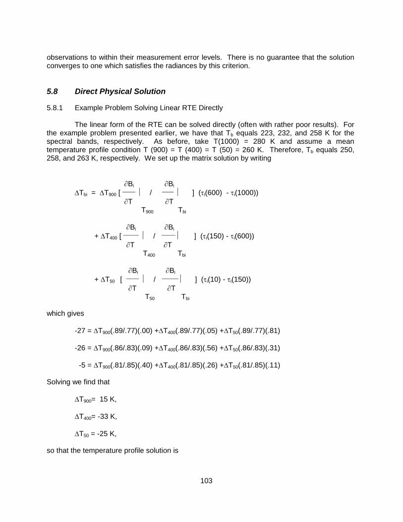
103
observations to within their measurement error levels. There is no guarantee that the solution converges to one which satisfies the radiances by this criterion.
5.8 Direct Physical Solution
5.8.1 Example Problem Solving Linear RTE Directly
The linear form of the RTE can be solved directly (often with rather poor results). For the example problem presented earlier, we have that Tb equals 223, 232, and 258 K for the spectral bands, respectively. As before, take T(1000) = 280 K and assume a mean temperature profile condition T (900) = T (400) = T (50) = 260 K. Therefore, Tb equals 250, 258, and 263 K, respectively. We set up the matrix solution by writing
Bi Bi
Tbi = T900 [
/
] (i(600) - i(1000))
T T T900 Tbi
Bi Bi
+ T400 [
/
] (i(150) - i(600))
T T T400 Tbi
Bi Bi
+ T50 [
/
] (i(10) - i(150))
T T T50 Tbi
which gives
-27 = T900(.89/.77)(.00) +T400(.89/.77)(.05) +T50(.89/.77)(.81)
-26 = T900(.86/.83)(.09) +T400(.86/.83)(.56) +T50(.86/.83)(.31)
-5 = T900(.81/.85)(.40) +T400(.81/.85)(.26) +T50(.81/.85)(.11) Solving we find that
T900= 15 K,
T400= -33 K,
T50 = -25 K, so that the temperature profile solution is

104
T(900) = 275 K,
T(400) = 227 K,
T(50) = 235 K. Obviously, this example was ill-conditioned since Taylor expansion of differences larger than 10 K is foolhardy. However, this does demonstrate how to set up a direct solution, which should
be representative of the mean temperature condition used in the expansion is close to the actual temperature profile.
Typically, the direct solution is unstable because there are the unknown observation errors and W is nearly singular due to strong overlapping of the weighting functions. Since W is ill-conditioned with respect to matrix inversion, the elements of the inverse matrix are greatly inflated which, in turn, greatly amplifies the experimental error of the observations. This renders the solution virtually useless. The ill-conditioned solution results since one does not have N independent pieces of information about T from M radiation observations. The solution is further complicated because M is usually much smaller than the number of temperature points, N, needed to represent the temperature profile. 5.8.2 Simultaneous Direct Physical Solution of the RTE for Temperature and Moisture
Solution of the RTE often involves several iterations between solving for the temperature and moisture profiles. As pointed out earlier, they are interrelated but most solutions only solve for each one separately, assuming the other is known. Recently Smith (1985) has developed a simultaneous direct physical solution of both.
In order to solve for the temperature and moisture profiles simultaneously, a simplified form of the integral of the radiative transfer equation is considered,
ps R = Bo + dB
o
which comes integrating the atmospheric term by parts in the more familiar form of the RTE. R
represents the radiance, the transmittance, and B the Planck radiance. Dependency on angle, pressure, and frequency are neglected for simplicity. The subscript s refers to the
surface level and o refers to the top of the atmosphere. Then in perturbation form, where represents a perturbation with respect to an a priori condition
ps ps
R = () dB + d(B) . o o
Integrating the second term on right side of the equation by parts,
ps ps ps ps d(B) = B - B d = s Bs - B d , o o o o

105
yields
ps ps R = () dB + s Bs - B d
o o Now writing the differentials with respect to temperature
B B R = Tb
, B = T
____
Tb T and with respect to pressure
B T dB =
dp , d =
dp ,
T p p yields
ps T B B ps B B Tb =
[
/
] dp - T
[
/
] dp
o p T Tb o p T Tb
Bs B + Ts [
/
] s
Ts Tb where Tb is the brightness temperature. Finally, assume that the transmittance perturbation is dependent only on the uncertainty in the column of precipitable water density weighted path length u according to the relation
=
u .
u Thus
ps T B B p τ B B Tb = u
[
/
] dp - T
[
/
] dp
o p u T Tb o p T Tb
Bs B + Ts [
/
] s
Ts Tb
= f [ u, T, Ts ] where f represents a functional relationship.
The perturbations are with respect to some a priori condition which may be estimated from climatology, regression, or more commonly from an analysis or forecast provided by a numerical model. In order to solve for u, T, and Ts from a set spectrally independent radiance observations Tb, the perturbation profiles are represented in terms of arbitrary basis functions φ (p); so
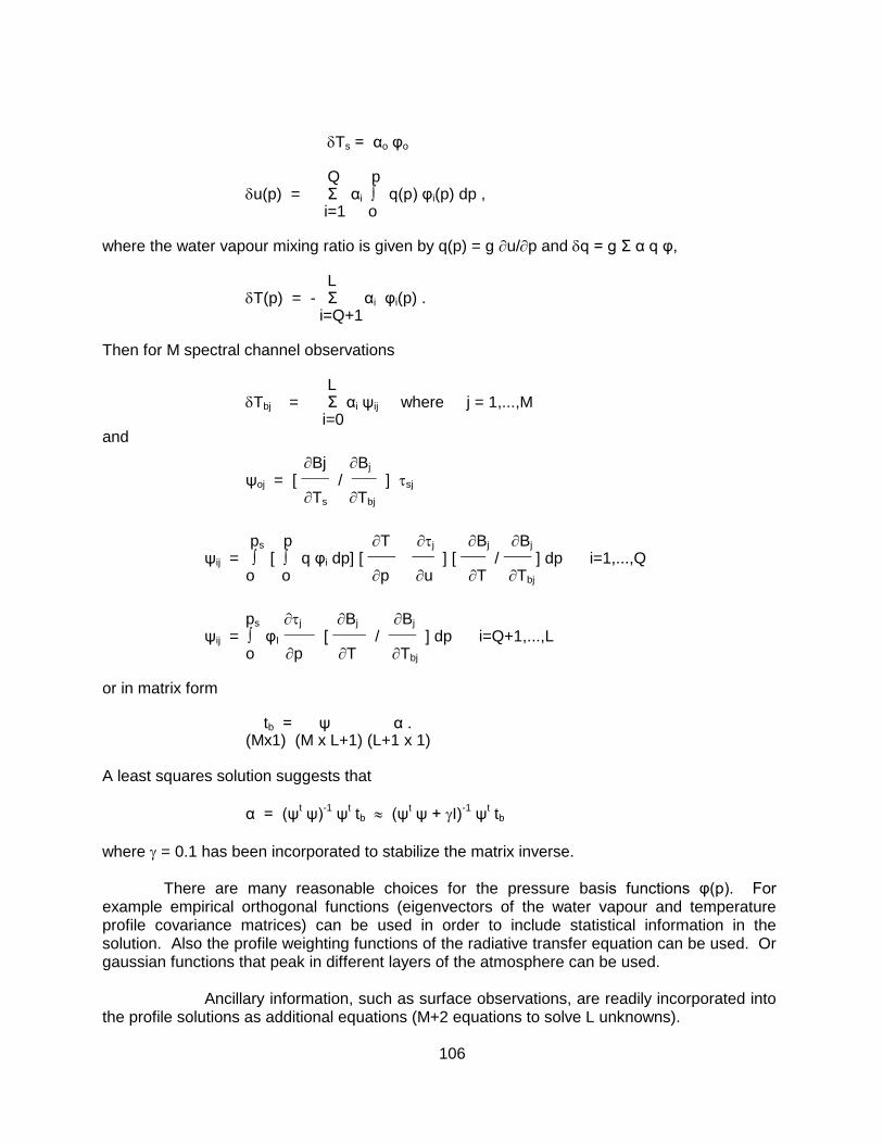
106
Ts = αo φo
Q p
u(p) = Σ αi q(p) φi(p) dp , i=1 o
where the water vapour mixing ratio is given by q(p) = g u/p and q = g Σ α q φ,
L
T(p) = - Σ αi φi(p) . i=Q+1
Then for M spectral channel observations
L
Tbj = Σ αi ψij where j = 1,...,M i=0
and
Bj Bj ψoj = [
/
] sj
Ts Tbj
ps p T j Bj Bj
ψij = [ q φi dp] [
] [
/
] dp i=1,...,Q o o p u T Tbj
ps j Bj Bj
ψij = φI
[
/
] dp i=Q+1,...,L o p T Tbj
or in matrix form
tb = ψ α . (Mx1) (M x L+1) (L+1 x 1)
A least squares solution suggests that
α = (ψt ψ)
-1 ψ
t tb (ψ
t ψ + I)
-1 ψ
t tb
where = 0.1 has been incorporated to stabilize the matrix inverse.
There are many reasonable choices for the pressure basis functions φ(p). For example empirical orthogonal functions (eigenvectors of the water vapour and temperature profile covariance matrices) can be used in order to include statistical information in the solution. Also the profile weighting functions of the radiative transfer equation can be used. Or gaussian functions that peak in different layers of the atmosphere can be used. Ancillary information, such as surface observations, are readily incorporated into the profile solutions as additional equations (M+2 equations to solve L unknowns).

107
Q qo - q (ps) = g Σ αi q(ps) φi(ps)
i=1
L To - T (ps) = - Σ αi φi(ps)
i=Q+1 In summary we have the following characteristics (a) the RTE is in perturbation form, (b) T and u are expressed as linear expansions of basis functions (EOF or W(p)), (c) ancillary observations are used as extra equations, (d) a least squares solution is sought, and (e) a simultaneous temperature and moisture profile solution produces improved moisture determinations. The simultaneous solution addresses the interdependence of water vapour radiance upon temperature and carbon dioxide channel radiance upon water vapour concentration. The dependence of the radiance observations on the surface emissions is accounted for by the inclusion of surface temperature as an unknown. A single matrix solution is computationally efficient compared to an iterative calculation.
5.9 Water Vapour Profile Solutions
The direct physical solution of the RTE provides a simultaneous solution of both the temperature and moisture profiles. It is currently the preferred solution. On the other hand, iterative numerical techniques involve several determinations of each profile separately before self consistent convergence is achieved. The iterative numerical solution for the moisture profile is presented here. It should be viewed as a companion to the iterative numerical solution of the temperature profile presented in section 5.7.
The linear form of the RTE can be written in terms of the precipitable water vapour profile as
us (Tb)λ = (T) Vλ du
o where
Bλ(T) Bλ(T) λ Vλ = [
| /
| ]
______
T T u T=Tav T=Tbλ
and Tav(p) represents a mean or initial profile condition.
One manner of solving for the water vapour profile from a set of spectrally independent water vapour radiance observations is to employ one of the linear direct temperature profile solutions discussed earlier. In this case, however, one solves for the function T(u) rather than T(p). Given T(p) from a prior solution of carbon dioxide and/or oxygen channel radiance observations, u(p) can be found by relating T(p) to T(u). The mixing ratio profile, q(p), can then be obtained by taking the vertical derivative of u(p), q(p) = g u/p where g is gravity.
Rosenkranz et al (1982) have applied this technique to microwave measurements of water vapour emission. They used the regression solution for both the temperature versus pressure and temperature versus water vapour concentration profiles. The regression solutions have the form

108
N
T(pj) = to(pj) + Σ ti(pi) Tbi i=1
and M
T(uk) = to(uk) + Σ tm(uk) Tbm m=1
where Tbi are the N brightness temperature observations of oxygen emission and Tbm are the M brightness temperature observations of water vapour emission and ti(pj) and tm(uk) are the regression coefficients corresponding to each pressure and water vapour concentration level. u(p) is found from the intersections of the T(p) and T(u) profiles obtained by interpolation of the discrete values given by the regression solutions. An advantage of the linear regression retrievals is that they minimize the computer requirements for real time data processing since the regression coefficient matrices are predetermined.
Various non-linear iterative retrieval methods for inferring water vapour profiles have also been developed and applied to satellite water vapour spectral radiance observations by Smith (1970).
5.10 Microwave Form of RTE
In the microwave region, the emissivity of the earth atmosphere system is normally less than unity. Thus, there is a reflection contribution from the surface. The radiance emitted from the surface would therefore be given by
ps
↓λ(p)
Iλ sfc
= ελ Bλ(Ts) λ(ps) + (1-ελ) λ(ps) Bλ(T(p))
d ln p o ln p
The first term in the right-hand side denotes the surface emission contribution,
whereas the second term represents the emission contribution from the entire atmosphere to the surface, which is reflected back to the atmosphere at the same frequency. The transmittance
↓λ(p) is now expressed with respect to the surface instead of the top of the
atmosphere (as λ (p) is). Thus, the upwelling radiance is now expressed as ps
↓λ(p)
Iλ = ελ Bλ(Ts) λ(ps) + (1-ελ) λ(ps) Bλ(T(p))
d ln p o ln p
o λ(p) + Bλ(T(p))
d ln p
ps ln p In the wavelength domain, the Planck function is given by
c2/λT Bλ(T) = c1 / [ λ
5 (e - 1) ] .
In the microwave region c2 /λT << 1, so the Planck function may be approximated by

109
c1 T
Bλ(T)
; c2 λ
4
the Planck radiance is linearly proportional to the temperature. Analogous to the above approximation, we may define an equivalent brightness temperature Tb such that
c1 Tb Iλ =
.
c2 λ4
Thus, the microwave radiative transfer equation may now be written in terms of temperature
ps ↓λ(p)
Tbλ = ελ Ts λ(ps) + (1-ελ) λ(ps) T(p)
d ln p o ln p
o λ(p) + T(p)
d ln p .
ps ln p The transmittance to the surface can be expressed in terms of transmittance to the top of the atmosphere by remembering 1 ps
↓λ(p) = exp [ -
kλ(p) g(p) dp ]
g p
ps p = exp [ - + ] o o
= λ(ps) / λ(p) .
So
↓λ(p) λ(ps) λ(p)
= -
. ln p (λ(p))
2 ln p
And thus to achieve a form similar to that of the infrared RTE, we write o λ(p)
Tbλ = ελ Ts(ps) λ(ps) + T(p) Fλ(p)
d ln p ps ln p
where
λ(ps) Fλ(p) = { 1 + (1 - ελ) [
]2 } .
λ(p)

110
A special problem area in the use of microwave for atmospheric sounding from a satellite platform is surface emissivity. In the microwave spectrum, emissivity values of the earth's surface vary over a considerable range, from about 0.4 to 1.0. The emissivity of the sea surface typically ranges between 0.4 and 0.5, depending upon such variables as salinity, sea ice, surface roughness, and sea foam. In addition, there is a frequency, dependence with higher frequencies displaying higher emissivity values. Over land, the emissivity depends on the moisture content of the soil. Wetting of a soil surface results in a rapid decrease in emissivity. The emissivity of dry soil is on the order of 0.95 to 0.97, while for wet bare soil it is about 0.80 to 0.90, depending on the frequency. The surface emissivity appearing in the first term has a significant effect on the brightness temperature value.
The basic concept of inferring atmospheric temperatures from satellite observations of thermal microwave emission in the oxygen spectrum was developed by Meeks and Lilley (1963) in whose work the microwave weighting functions were first calculated. The prime advantage of microwave over infrared temperature sounders is that the longer wavelength microwaves are much less influenced by clouds and precipitation. Consequently, microwave sounders can be effectively utilized to infer atmospheric temperatures in all weather conditions. We will not pursue microwave retrievals in this course, except to say that the techniques are similar to those for infrared retrieval.

111
High
Mid
Low
ABC
A
B
C
MODIS IR Spectral Bands
MODIS
A B C
Figure 5.1: Location of three spectral bands in the CO2 absorption band at 15 um (left), pressure broadening of the absorption line from high to low in the atmosphere with the spectral band locations indicated (center), and vertical distribution of the weighting functions for the three spectral bands (right).
CO2 channels see to different levels in the atmosphere
14.2 um 13.9 um 13.6 um 13.3 um
Figure 5.2: Images of measurements in the CO2 spectral region from very opaque (left) to nearly transparent (right).

112
Figure 5.3: Outgoing radiance in terms of black body temperature in the vicinity of 15μm CO2 band observed by the IRIS on Nimbus IV. The arrows denote the spectral regions sampled by the VTPR instrument.
Figure 5.4: Temperature retrieval using Chahine's relaxation and Smith's iterative methods for the VTPR channels.

113
CHAPTER 6
CLOUDS 6.1 RTE in Cloudy Conditions
Thus far, we have considered the RTE only in clear sky conditions. When we introduce clouds into the radiation field of the atmosphere the problem becomes more complex. The following notes indicate some of the fundamental problems concerning clouds.
If we assume that the fractional cloud cover within the field of view of the satellite radiometer is represented by η and the cloud top pressure by pc, then the spectral radiance measured by the satellite radiometer at the top of the atmosphere is given by
Iλ = η Icd
+ (1 - η) Ic
λ λ
where cd denotes cloud and c denotes clear. As before, we can write for the clear radiance
o I
c = Bλ(Ts) λ(ps) + Bλ(T(p)) dλ .
λ ps
The cloud radiance is represented by pc
Icd
= (1-ελ) Bλ(Ts) λ(ps) + (1-ελ) Bλ(T(p)) dλ
λ ps
o
+ ελ Bλ(T(pc)) λ(pc) + Bλ(T(p)) dλ pc
where ελ represents the emittance of the cloud. The first two terms are contributions from below the cloud, the third term is the cloud contribution, and the fourth term is the contribution from above the cloud. After some rearranging these expressions can be combined to yield
Iλ - Iλc = η (Iλ
cd - Iλ
c)
pc
= η ελ [ Bλ(T(pc)) λ(pc) - Bλ(Ts) λ(ps) - Bλ(T(p)) dλ ] ps A simpler form is available by using integration by parts, so
pc dBλ Iλ - Iλ
c = ηελ (p) dp .
ps dp

114
The techniques for dealing with clouds generally fall into three different categories: (a) searching for cloudless fields of view, (b) specifying cloud top pressure and sounding down to cloud level as in the cloudless case, and (c) employing adjacent fields of view to determine the clear sky signal from partly cloudy observations.
6.2 Inferring Clear Sky Radiances in Cloudy Conditions
The adjacent fields of view technique proceeds as follows. For a given wavelength λ, the radiances from two spatially independent, but geographically close, fields of view are written
Iλ,1 = η1 Iλ,1
cd + (1 - η1) Iλ,1
c ,
Iλ,2 = η2 Iλ,2
cd + (1 - η2) Iλ,2
c ,
If the clouds have a uniform altitude, and the clear air radiance is the same from the
two yields of view
Iλcd
= Iλ,1cd
= Iλ,2 cd
and
Iλc = Iλ,1
c = Iλ,2
c
then cd c c
η1 (Iλ - Iλ ) η1 Iλ,1 - Iλ
=
= η* =
,
cd c c η2 (Iλ - Iλ) η2 Iλ,2 - Iλ
where η* is the ratio of the cloud amounts for the two geographically independent fields of view of the sounding radiometer. Therefore, the clear air radiance from an area possessing broken clouds at a uniform altitude is given by
c Iλ,1 - η* Iλ,2
Iλ = ________________
1 - η*
where η* still needs to be determined. Given an independent measurement of the surface temperature, Ts, and measurements Iw,1 and Iw,2 in a spectral window channel, then η* can be determined by
Iw,1 - Bw(Ts) η* =
____________________
Iw,2 - Bw(Ts) and Iλ
c for the different spectral channels can be solved. Another approach to determining η* is
to use simultaneous microwave observations and regression relations between a lower tropospheric microwave sounding brightness temperature and the associated infrared brightness temperatures observed for cloud-free conditions. So if

115
Imw = Σ aλ Iλ
c ,
λ then
Iλ,1- η* Iλ,2 Imw = Σ aλ
,
λ 1 - η* and
Imw - Σ aλ Iλ,1 λ
η* = .
Imw - Σ aλ Iλ,2
λ The partly cloud η* solution has been the basis of the design of the operational infrared sounders (VTPR, ITPR, HIRS, VAS, and GOES Sounder). The technique is largely credited to Smith. With this correction for cloud contamination, a solution for the temperature profile can be pursued using the techniques presented in this chapter 5.
When there is a differing amount of the same cloud present in two adjacent or nearby fields of view, the cloud corrected radiance is available from the 3.7 and 11.0 micron infrared windows (when reflected sunlight does not interfere with the observations in the shortwave region). Given a partly cloudy atmospheric column then the ratio of the cloud fraction in the two FOVs, η*, can be estimated from each window channel separately viewing two adjacent fields of view as before
Iw1,1 - Bw1(Ts) Iw2,1 - Bw2(Ts) η* =
=
.
Iw1,2 - Bw1(Ts) Iw2,2 - Bw2(Ts) Ts is the value that satisfies this equality. Also one can show that
Bw1(Ts) = Ao + A1 Bw2(Ts) where
Iw2,1 Iw1,2 - Iw1,1 Iw2,2 Ao =
_______________________
Iw2,1 - Iw2,2 and
Iw1,1 - Iw1,2 A1 =
_____________
Iw2,1 - Iw2,2
For constant cloud height and surface temperature conditions, the observed radiances for the two window channels will both vary linearly with cloud amount. As a consequence, cloud amount variations produces a linear variation of the radiance observed in one window channel relative to that radiance observed in another window channel. This linear relation can be used to determine the value of the window radiances for zero cloud amount (N = 0). As

116
shown in Figure 6.1, zero cloud amount must be at the intersection of the observed linear relationship and the known Planck radiance relationship. The brightness temperature associated with this point is the surface temperature. Another common point for the observed and Planck functions is for the case of complete overcast cloud (N = 1). The brightness temperature associated with this point is the cloud temperature. It follows that the constants of the observed linear relationship are the Ao and A1 constants of the previous equation.
6.3 Finding Clouds
Clouds are generally characterized by higher reflectance and lower temperature than the underlying earth surface. As such, simple visible and infrared window threshold approaches offer considerable skill in cloud detection. However there are many surface conditions when this characterization of clouds is inappropriate, most notably over snow and ice. Additionally, some cloud types such as cirrus, low stratus, and roll cumulus are difficult to detect because of insufficient contrast with the surface radiance. Cloud edges cause further difficulty since the field of view is partly cloudy and partly clear. Multispectral approaches offer several opportunities for improved cloud detection so that many of these concerns can be mitigated. Finally, spatial and temporal consistency tests offer confirmation of cloudy or clear sky conditions.
The purpose of a cloud mask is to indicate whether a given view of the earth surface is
unobstructed by clouds. The question of obstruction by aerosols is somewhat more difficult and will be addressed only in passing. This chapter describes algorithms for cloud detection and details multispectral applications for cloud properties. Several references are listed as suggested reading regarding cloud detection: Ackerman et al, 1998; Gao et al, 1993; King et al, 1992; Rossow and Garder, 1993; Stowe et al, 1991; Strabala et al, 1994; and Wylie and Menzel, 1999.
In the following sections, the satellite measured visible (VIS) reflectance is denoted as
r and the infrared (IR) radiance is described by its brightness temperature (equivalent blackbody temperature using the Planck function) denoted as Tb. Subscripts refer to the wavelength at which the measurement is made. 6.3.1 Threshold and Difference Tests to Find Clouds
As many as eight single field of view (FOV) cloud mask tests are indicated for daylight conditions (given that the sensor has the appropriate spectral channels). Many of the single FOV tests rely on infrared radiance (temperature) and visible reflectance thresholds that vary with surface emissivity, atmospheric moisture, aerosol content, and viewing scan angle.
(a) IR Window Temperature Threshold and Difference Tests
Several infrared window threshold and temperature difference techniques are used. Thresholds will vary with moisture content of the atmosphere as the longwave infrared windows exhibit some water vapour absorption (see Figure 6.2). Threshold cloud detection techniques are most effective at night over water. Over land, the threshold approach is further complicated by the fact that the emissivity in the infrared window varies appreciably with soil and vegetation type (see Figure 6.3). Over ocean when the brightness temperature in the 11 micron channel (Tb11) is less than 270 K, we can safely assume a cloud is present. As a result of the relative

117
spectral uniformity of surface emittance in the IR, spectral tests within various atmospheric windows (such as those at 8.6, 11, and 12 microns respectively) can be used to detect the presence of a cloud. Differences between Tb11 and Tb12 have been widely used for cloud screening with AVHRR measurements and this technique is often referred to as the split window technique.
The anticipation is that the threshold techniques will be very sensitive to thin clouds, given the appropriate characterization of surface emissivity and temperature. For example, with a surface at 300 K and a cloud at 220 K, a cloud with emissivity at 0.01 reduces the sensed brightness temperature by 0.5 K. Since the noise equivalent temperature of many current infrared window channels is 0.1 K, the cloud detecting capability is obviously very good.
The split window technique for cloud detection is based on the differential water
vapour absorption that exists between the window channels (8.6 and 11 micron and 11 and 12 micron). These spectral regions are considered to be part of the atmospheric window, where absorption is relatively weak (see Figure 6.2). Most of the absorption lines are caused by water vapour molecules. Since the absorption is weakest around 11 microns, Tb11 can be corrected for moisture absorption in a linear approximation by adding the scaled brightness temperature difference of two spectrally close channels with different water vapour absorption coefficients; the scaling coefficient is a function of the differential water vapour absorption between the two channels. This is the basis for sea surface temperature retrievals (see Chapter 6). Thus Ts = Tbλ1 + aPW (Tbλ1 - Tbλ2) , where aPW is a function of wavelengths of the two window channels and the total precipitable water vapour in the atmosphere.
Thus, given an estimate of the surface temperature, Ts, and the total precipitable water vapour, PW, one can develop appropriate thresholds for cloud detection
Tb11 < 270 K ,
Tb11 + aPW (Tb11 - Tb12) < Ts ,
Tb11 + bPW (Tb11 - Tb8.6) < Ts , where aPW and bPW are determined from a look up table as a function of total precipitable water vapour. This approach has been used operationally for many years using 8.6 and 11 micron spectral bands from the NOAA-10 and NOAA-12 and the 11 and 12 micron spectral bands from the NOAA-11, with a coefficient independent of PW (Menzel et al 1993, Wylie et al 1994).
The dependence on PW of the brightness temperature difference between the various window channels is seen in Figure 6.4. A global data set of collocated AVHRR 11 and 12 micron and HIRS 8.6 and 11 micron scenes were collected and the total column PW estimated from integrated model mixing ratios to determine a direct regression between PW and the split window thresholds. Linear regression fits indicate the appropriate values for aPW and bPW.
One disadvantage of the split window brightness temperature difference approach is that water vapour absorption across the window is not linearly dependent on PW, thus second order relationships are sometimes needed. With the measurements at three wavelengths in

118
the infrared window (8.6, 11, and 12 microns), this becomes less problematic; these three spectral regions are very useful in determining the presence of a cloud free atmosphere. This is because the index of refraction varies quite markedly over this spectral region for water, ice, and minerals common to many naturally occurring aerosols. As a result, the effect on the brightness temperature of each spectral band is different, depending on the absorbing constituent. Figure 6.5 summarizes the behaviour of the thresholds for different atmospheric conditions.
A tri-spectral combination of observations at 8.6, 11 and 12 microns was suggested for detecting cloud and cloud properties by Ackerman et al. (1990). Strabala et al. (1994) further explored this technique by utilizing very high spatial resolution data from a 50 channel mutltispectral radiometer called the MODIS Airborne Simulator (MAS). The premise of the technique is that ice and water vapour absorption is larger in the window region beyond 10.5 microns (see Figure 6.6); so that positive 8.6 minus 11 micron brightness temperature differences indicate cloud while negative differences, over oceans, indicate clear sky. The relationship between the two brightness temperature differences and clear sky have also been examined using collocated HIRS and AVHRR GAC global ocean data sets (as shown in Figure 6.7). As the atmospheric moisture increases, Tb8.6 - Tb11 decreases while Tb11 - Tb12 increases.
The shortwave infrared window channel at 3.9 microns offers another opportunity to detect the presence of clouds. At night Tb3.9-Tb11, the difference between the brightness temperatures measured in the shortwave (3.9 micron) and in the longwave (11 micron) window regions, can be used to detect partial cloud or thin cloud within the sensor field of view. Small or negative differences are observed only when an opaque scene (such as thick cloud or the surface) fills the sensor field of view. Negative differences occur at night over extended clouds due to the lower cloud emissivity at 3.9 microns. Moderate to large differences result when a non-uniform scene (e.g., broken cloud) is observed. This brightness temperature difference is a result of Planck's law; the brightness temperature of the warmer portion of the scene increases with decreasing wavelength (the shortwave window Planck radiance is proportional to temperature to the thirteenth power, while the longwave window dependence is to the fourth power). Table 6.1 gives an example of radiances (and brightness temperatures) observed for different cloud fractions in a scene where cold cloud partially obscures warm surface. Differences in the brightness temperatures of the longwave and shortwave channels are small when viewing mostly clear or mostly cloudy scenes; however for intermediate situations the differences become quite large. It is worth noting in Table 6.1 that the brightness temperature of the shortwave window channel is relatively insensitive to small amounts of cloud (compared to the longwave window channel), thus making it the preferred channel for surface temperature determinations.
Cloud masking over land surfaces from thermal infrared bands is more difficult than over ocean due to larger variations in surface emissivities (see Figure 6.3 and Table 6.2). Nonetheless, simple thresholds can be established over certain land features. For example, over desert regions we can expect that Tb11 < 273 K indicates cloud. Such simple thresholds will vary with ecosystem, season, and time of day.
Brightness temperature difference testing can also be applied over land after careful consideration of variations in spectral emissivity. For example, Tb11 - Tb8.6 has large negative values over daytime desert but exhibit positive values in the presence of cirrus. Some land regions have an advantage over the ocean regions because of the larger number of surface observations, which include air temperature, and vertical profiles of moisture and temperature.

119
Infrared window tests at high latitudes are difficult. Distinguishing clear and cloud
regions from satellite IR radiances is a challenging problem when cold surface temperatures are present. Yamanouchi et al. (1987) describe a nighttime polar (Antarctic) cloud/surface discrimination algorithm based upon brightness temperature differences between the AVHRR 3.7 and 11 micron bands and between the 11 and 12 micron bands. Their cloud/surface discrimination algorithm was more effective over water surfaces than over inland snow-covered surfaces. A number of problems arose over inland snow-covered surfaces. First, the temperature contrast between the cloud and snow surfaces became especially small, leading to a small brightness temperature difference between the two infrared bands. Second, the AVHRR spectral bands are not well-calibrated at extremely cold temperatures (< 200 K). Under clear sky conditions, surface radiative temperature inversions often exist. Thus, IR spectral bands with weighting function peaks low in the atmosphere will often have a warmer brightness temperature than an IR window (e.g. Tb8.6 > Tb11 in the presence of an inversion). The surface inversion can also be confused with thick cirrus cloud, but this can be mitigated by other tests (e.g., the magnitude of Tb11 or Tb11-Tb12). Recent analysis of Tb11-Tb6.7 (the 6.7 micron water vapour channel peaks around 400 mb) has shown large negative differences in winter time over the Antarctic Plateau and Greenland that may be indicative of a strong surface inversion and thus clear skies. (b) CO2 Channel Test for High Clouds
A spectral channel sensitive to CO2 absorption at 13.9 micron provides good sensitivity
to the relatively cold regions of the atmosphere. The weighting function peaks near 300 hPa, so that only clouds above 500 hPa will have strong contributions to the radiance to space observed at 13.9 microns; negligible contributions come from the earth surface. Thus a 13.9 micron brightness temperature threshold test for cloud versus ambient atmosphere can reveal clouds above 500 hPa. This test should be used in conjunction with the near infrared thin cirrus test, described next. (c) Near Infrared Thin Cirrus Test
This relatively new approach to cirrus detection is suggested by the work of Gao et al (1993). A near infrared channel sensitive to H2O absorption at 1.38 microns can be used in reflectance threshold tests to detect the presence of thin cirrus cloud in the upper troposphere under daytime viewing conditions. This cloud detection test relies on the strong water vapour absorption in the 1.38 micron region. When sufficient atmospheric water vapour is present (estimated to be about 0.4 cm precipitable water) in the beam path, no upwelling reflected radiance from the earth's surface reaches the satellite. The transmittance is given by
(psfc) = exp(-H2O * secθo - H2O * secθ)
H2O = kH2O du
As (psfc) 0, rsfc 0. is the two-way atmospheric transmittance from the top of the
atmosphere down to the surface and back to the top of the atmosphere, H2O is the water vapour optical depth, θo and θ are the solar and viewing zenith angles respectively, kH2O is the water vapour absorption coefficient, u is the water vapour path length and rsfc is the surface radiance reaching the sensor. Since 0.4 cm represents a small amount of atmospheric water vapor, most of the earth's surface will be obscured in this channel. With relatively little of the

120
atmosphere's moisture located high in the troposphere, high clouds appear bright and unobscured in the channel; reflectance from low and mid level clouds is partially attenuated by water vapour absorption.
Simple low and high reflectance (normalized by incoming solar at the top of the atmosphere) thresholds can be used to separate thin cirrus from clear and thick (near infrared cloud optical depth > ~ 0.2) cloud scenes. These thresholds are set initially using a multiple-scattering model. New injections of volcanic aerosols into the stratosphere impact the thresholds, which require periodic adjustment. Any ambiguity of high thin versus low or mid level thick cloud is resolved by a test on the cloud height using a CO2 sensitive channel at 13.9 microns (see the previous section). (d) Shortwave Infrared Window Reflectance Threshold Test
One reflectance threshold test uses the 3.9 micron channel where values > 6% are considered to be cloudy. However, values < 3% are considered to be snow/ice (Stowe et al, 1994). Note that this reflectance test cannot be applied over deserts, as bright desert regions with highly variable emissivities tend to be classified incorrectly as cloudy. Thermal contrast needs to be examined in conjunction with 3.9 micron reflectivity. In addition, thresholds must be adjusted to ecosystem type because of the different surface emissivities (see Table 6.2). (e) Reflectance Threshold Test
Visible thresholds tests are best used in combination with infrared window observations; during daytime they can be combined as follows. Low reflectance measurements will result from thin cirrus cloud or cloud free conditions, the two being easily separable in the infrared window measurements by the large difference in the emitting temperature of the high cold cirrus and the warm underlying surface. High reflectance measurements result from thick clouds at all levels, and the infrared window brightness temperature provides a good indication of the cloud level. Intermediate reflectance data are subject to ambiguous interpretations since they result from a mixture of cloud and surface contributions.
Visible data used in the determination of the cloud mask must be free from sun glint. Algorithms which include solar reflectance data are constrained to solar zenith angles less than 85°. Sun glint occurs when the reflected sun angle, θr, lies between 0° and approximately 36°, where
cosθr = sinθ sinθo cos + cosθ cosθo
and θo is the solar zenith angle, θ is the viewing zenith angle, and is the azimuthal angle. Sun glint is also a function of surface wind and sea state. (f) Reflectance Ratio Test
The reflectance ratio test takes advantage of the difference in reflection from cloud versus earth surface in wavelengths above and below 0.75 microns. Many earth surfaces are less reflecting below 0.75 microns than above, but clouds do not exhibit any great difference in reflectance. Figure 6.8 shows the albedo variations for ice, snow, and vegetation from 0.5 to 3.5 microns. Vegetation shows a sharp increase above 0.72 microns. Snow/ice shows a sharp decrease above 1.4 microns. These step function changes are useful in detecting vegetation

121
or snow/ice versus clouds with spectral band pairs above and below the change. One version of the reflectance ratio test uses the 0.87 micron reflectance divided by 0.66 micron reflectance (r.87/r.66). With AVHRR data, this ratio has been found to be between 0.9 and 1.1 in cloudy regions. If the ratio falls within this range, cloud is indicated. McClain (1993) suggests that the minimum value may need to be lowered to about 0.8, at least for some cases. For cloud-free ocean, the ratio is expected to be less than 0.75 (Saunders and Kriebel, 1988). (g) Low Cloud Test
Clouds that are low in the atmosphere are often difficult to detect. The thermal contrast between clear sky and low cloud is small and sometimes undetectable by infrared techniques. Reflectance techniques, including the Reflectance Ratio Test (see previous section) can be applied during daylight hours. Use of a channel at 0.936 microns also offers help under daytime viewing conditions. As documented by Gao and Goetz (1991), this channel is strongly affected by low level moisture. When low clouds are present they obstruct the low level moisture, hence increasing the reflectance. A reflectance ratio of 0.936 over 0.865 microns, an atmospheric window with similar surface reflectance characteristics, also shows promise. (h) Microwave Tests
As noted earlier in section 6.2, the brightness temperature of a lower tropospheric sounding microwave channel can be regressed against the brightness temperatures of several lower tropospheric infrared sounding channels for clear situations. Therefore the microwave brightness temperature for a given FOV can be calculated from the observed infrared brightness temperatures. This will be valid in clear sky conditions only. If the observed microwave brightness temperature is greater than the calculated, it is indicative of cloud contamination in the infrared observations and the fov should be classified accordingly. (i) Resultant Cloud Mask
All of the single pixel tests mentioned so far rely on thresholds. Thresholds are never global. There are always exceptions and the thresholds must be interpreted carefully. For example, the reflectance ratio test identifies cloud for values in the range 0.9 to 1.1. However, it seems unrealistic to label a pixel with the ratio of 1.1 as cloudy, and a neighbouring pixel with the ratio of 1.11 as non-cloudy. Rather, as one approaches the threshold limits, the certainty or confidence in the labelling becomes more uncertain. An individual confidence flag is assigned with each of the single pixel test results and these are used in combination to work towards a final determination.
Each threshold determination is classified as pass, conditional pass, or fail along with a confidence assessment. Conditional pass involves those radiances that fall within an uncertainty region of the threshold. The uncertainty is a measure of instrument noise and the magnitude of the correction due to non blackbody surface emissivity as well as atmospheric moisture and/or aerosol reflection contributions. The individual confidence flag indicates a one, two, or three sigma confidence level for each single pixel test result. The initial FOV determination of cloudy or clear is a sum of the squares of all the confidence flags and single pixel test results.

122
6.3.2 Spatial Uniformity Tests for Finding Clouds
When the single field of view tests do not produce definitive determination of an unobstructed FOV, spatial and temporal consistency tests are often found to be useful. Temporal consistency compares the composited previous 30 day clear sky radiances and yesterday's cloud mask to today's clear sky single pixel results. Spatial consistency checks neighbouring clear sky pixel radiances (within the same ecosystem). If any consistency test fails, the confidence in the final cloud/no cloud determination is reduced by 1 sigma level. (a) Infrared Window One-Dimensional Histogram Tests
One-dimensional histogram tests have a long history of determining clear sky scenes. As with the IR threshold tests, these are most effective over water and must be used with caution in other situations. The method is based on the assumption that for a uniform scene, such as a small geographic region of the ocean, the observed radiances will be normally distributed, with the width of the normal curve defined by the instrument noise. This is not a single FOV test, but requires many observations over a given region with similar surface radiative properties. To improve the clear sky estimate, the histogram is constructed only from the FOVs that pass one or more of the single FOV thresholds previously discussed. A one-dimensional histogram is constructed of the number of occurrences of discrete values of brightness temperature over a given geographical region (for 1km FOVs an area of 10 km x 10 km is appropriate). A gaussian function is fit to the warmest peak of the histogram; the temperature (Tpeak) and the noise limits (σ) are determined. The clear sky brightness temperature threshold is the temperature that corresponds to one-sigma (σ) towards the cold side of the gaussian function peak. Tthres = Tpeak - σ . An example of this approach is demonstrated in Figure 6.9 using AVHRR observations. (b) Infrared Window Radiance Spatial Uniformity
The infrared window spatial uniformity test (often applied on 10 by 10 pixel segments) is also most effective over water and must be used with caution in other situations. Most ocean regions are well suited for spatial uniformity tests; but such tests must be used with caution in coastal regions or regions with large temperature gradients (e.g. the Gulf Stream). The spatial coherence test is based on the assumption of a uniform background and singled-layered, optically thick cloud systems. The emitted radiance is given by I = (1 - Ac) Iclr + Ac Icld , where Ac represents the cloud fraction within the FOV. The method is based upon the computation of the mean and standard deviation for a group of pixels using 11 micron radiances. When the standard deviation is plotted versus the mean an arch shaped structure is often observed (see Figure 6.10). The feet with low standard deviations are associated with clear skies for high mean values and cloudy conditions for low mean values. The clear sky FOVs can be selected as those within a standard deviation threshold (which is fixed at a small value) of the warm foot of the arch. The derived clear sky foot of the arch should have a temperature consistent with the thresholds derived using the individual FOV tests. Uniform

123
stratus can also give the appearance of a uniform ocean, thus the spatial tests must often complement the threshold tests (e.g., the tri-spectral test).
Surface temperature variability, both spatial and temporal, is larger over land than ocean, making land scene spatial uniformity tests difficult. If the spatial uniformity tests over land are constrained to similar ecosystems, then better results are obtained.
The spatial coherence method developed by Coakley and Bretherton (1982) is recognized for being especially useful in determining clear and cloudy sky radiances over uniform backgrounds. It has been applied to single-layered and sometimes multi-layered cloud systems that extend over moderately large regions, greater than (250 km)
2, and which have
completely cloudy and completely clear pixels. The spatial coherence test is not run over regions of varying topography; however, it is applied for relatively homogeneous topographical regions of similar ecosystems. (c) Visible Reflectance Uniformity Test
A reflectance uniformity test can be applied by computing the maximum and minimum values of the 0.66 micron channel and the 0.87 micron channel reflectances within a 10 x 10 pixel array. Pixel arrays with 0.66 micron reflectance differences greater than threshold 1 (around 9%) over land or 0.87 micron reflectance differences greater than threshold 2 (possibly 0.3%) over ocean are labelled as mixed (Stowe et al., 1993). The value over ocean is low because a cloud-free ocean is almost uniformly reflective, while non-uniformity is assumed to be caused by cloudiness. This test again works better by requiring that the ecosystem be the same for the pixel array. Further, the reflectance threshold is a function of satellite zenith and view angle. (d) Two-Dimensional Infrared and Visible Histogram Analysis
As with the 1-D histogram approach, 2-D histograms can be constructed which make use of the measurements of IR emitted radiances as well as the reflected solar visible radiances. A 2-D Gaussian surface can be fitted to the peak with the warmest temperature and/or lowest reflectance. The Gaussian surface equation is
G(IR,VIS) = Gpeak exp[- P(IR,VIS)] with P(IR,VIS) = (Tb-Tbpeak)
2 /σIR
2 - 2(Tb-Tbpeak)(r-rpeak)/σIRσVIS + (r-rpeak)
2/σVIS
2
where σIR and σVIS are the IR and VIS standard deviations respectively. VIS channels may be replaced with NIR channels when necessary. The solar and infrared radiances can be a combination of various channels. The best solar channels to use are those for which the difference in reflectance between cloudy and clear sky is a maximum.
6.4 The Cloud Mask Algorithm
The tests detailed in the previous sections are applied as follows. Single pixel threshold tests are engaged first. If the confidence level reads uncertain (less than 2 sigma

124
confidence), then spatial uniformity tests on 10 by 10 pixel segments are used. Temporal and spatial continuity tests follow; these utilize data from 50 by 50 pixel segments, the cloud mask from yesterday, and the clear sky radiance composite from the last month.
6.4.1 Thick High Clouds (Group 1 Tests) Thick high clouds are detected with threshold tests that rely on BT11, BT13.9, and BT6.7. Infrared window thresholds, BT11, are practical under certain conditions, however they will vary with moisture content of the atmosphere. Over land, BT11 is further complicated by the fact that the surface emissivity varies appreciably with soil and vegetation type. Thus, BT11 is used primarily to detect high, thick clouds and thresholds are set accordingly. For example, clouds are likely present when BT11 is less than 270 K over tropical oceans. BT13.9 provides good sensitivity to the relatively cold regions of the atmosphere because of CO2 absorption. The same is true for BT6.7 because of H2O absorption. These spectral bands receive most of their radiation near 300 hPa and only clouds above 500 hPa make strong radiance contributions; negligible contributions come from the earth surface. Thus a threshold for BT13.9 and BT6.7 can isolate clouds above 500 hPa. 6.4.2 Thin Clouds (Group 2 Tests) Thin clouds tests rely on brightness temperature difference tests BT11- BT12, BT8.6- BT11, BT11- BT3.9, and, BT11- BT6.7. These tests will catch many of the clouds missed by the thick high cloud tests. Differences between BT11 and BT12 have been widely used for cloud screening with AVHRR measurements. For HIRS and MODIS, BT8.6 - BT11 greater than zero indicates cloud, while negative differences, over oceans, indicate clear regions. As atmospheric moisture increases, BT8.6 - BT11 decreases while BT11 - BT12 increases. Brightness temperature difference techniques for many of the infrared window spectral bands on the newer sensors with better than .05 K noise are being used successfully in thin clouds. At night positive values of BT3.9- BT11 are used to detect partial cloud or thin cloud within the sensor field of view. Negative differences occur over extended clouds due to the lower
cloud emissivity at 3.9 m. In daylight hours, solar reflection at 3.9 m is used for detecting water clouds. In polar regions during winter, large negative values in BT8.6 - BT11 during winter time over the Antarctic Plateau and Greenland indicate a strong surface inversion and thus clear skies. This test is proving useful in the MODIS cloud mask algorithm. 6.4.3 Low Clouds (Group 3 Tests) Low clouds are best detected using solar reflectance tests that include reflectance thresholds (r0.87, r0.65, and r0.936), reflectance ratio tests, and brightness temperature differences BT3.9- BT3.7. These tests work well when there is a high contrast in the reflectance between the surface and the cloud, for example, clouds over dark vegetation and water. Group 3 tests complement Group 1 tests; Group 3 is sensitive to thick, low level clouds while Group 1 has difficulty with low clouds that have small thermal contrast between cloud and background. Spectral reflectance thresholds are routinely used in many cloud detection algorithms. A wide

125
variety of thresholds exists in the literature, depending on surface type and solar and view angle geometry. Pre-launch threshold estimates require adjustment post-launch. The reflectance ratio (r0.87/r0.66) is between 0.9 and 1.1 in cloudy regions and outside in clear regions. The lower value is adjusted to below 0.75 for cloud-free ocean.
The shortwave infrared window bands at 3.7 and 3.9 m are also used to detect the presence of clouds. Over land, longwave infrared window spectral variation in surface emissivity presents difficulties for brightness temperature difference tests. Shortwave infrared window spectral variation in surface emissivity is much smaller for some ecosystems, while spectral variation in cloud emissivity remains substantial. Thus brightness temperature differences between BT3.7 and BT3.9 are usually small in clear skies but larger in clouds. During
the daylight hours the difference increases because of the increased solar energy at 3.7 m. 6.4.4 High Thin Clouds (Group 4 Tests)
Initial detection of high thin clouds is attempted with a threshold test at 1.38 m. No upwelling reflected radiance from the earth's surface reaches the sensor when sufficient atmospheric water vapor is present (estimated to be about 0.4 cm precipitable water) in the FOV. Simple low and high reflectance thresholds are used to separate thin cirrus from clear
and thick (near-infrared cloud optical depth > 0.2) cloud scenes.
Further detection of high thin cirrus is attempted with inspection of brightness temperature difference tests BT11- BT12, BT12- BT4, and BT13.7- BT13.9. The Group 4 tests are similar to those in Group 2, but they are specially tuned to detect the presence of thin cirrus. BT11- BT12 is positive in ice clouds due to the larger absorption at the longer wavelength in the infrared window. BT12- BT4 is negative in semitransparent cirrus as subpixel warm features dominate the shortwave window radiances within a FOV. BT13.7- BT13.9 is nominally positive in clear skies, but goes to zero when viewing cirrus. The large differences between ground and cloud temperatures make these tests useful for thin cirrus detection. 6.4.5 Ancillary Data Requirements
A number of preprocessing steps are necessary before a cloud masking algorithm can be applied. First, each pixel in the scene must be identified as being land or water, and if land, a land/water percentage must be estimated. Second, each land pixel must be designated as relatively flat, valley, isolated mountainous region, low mountains or hills, generally mountainous, or extremely rugged mountains. Each pixel must also be designated as probably/probably not snow covered. Each land pixel must be classified as to its ecosystem, along with a more general ecosystem classification of urban, forest, woodland, grassland, shrub land, tundra, arid vegetation and highland vegetation. Ocean regions must be classified as water, coastline (including islands), possibility of isolated icebergs, marginal ice zone, and nearly solid sea ice (leads may be present). This requires the ancillary data described below.
Earth surface character types are available in various databases which categorize features such as:
- salt or lake bed - flat or relatively flat desert (or for high latitudes, glaciers or permanent ice) - marsh

126
- lake country or atoll - major valleys or river beds - isolated mountains, ridge or peak - low mountains - mountainous - extremely rugged mountains - ocean
The different surface emissivities should be estimated according to different ecosystems. Table 6.5 shows some representative values for the infrared windows. Also Figure 6.3 provides further information.
Sea ice coverage is available from the US NAVY/NOAA Sea Ice Product, which provides weekly reports of fractional ice coverage at spatial resolution of about 18 km.
Snow cover is available in the NOAA Snow Data Product, which provides weekly reports of snow cover at a spatial resolution of 150-200 km; snow is reported if the grid cell is more than 50% covered.
Information on surface temperature and sea state is available from surface observations, Reynolds blended analysis, and NMC model 3-hour surface analyses of temperature and wind speed. 6.4.6 Implementing the Cloud Mask Algorithms
The cloud mask has the following stages: (a) Identify pixels that have sun glint (possible effect on visible tests); (b) Identify pixels that have high solar zenith angle (possible effect on visible tests); (c) Apply single FOV masking tests and set initial unobstructed FOV determination:
IR temperature threshold and difference tests; CO2 test for high clouds; Near infrared thin cirrus test; SWIR Reflectance threshold test; Reflectance ratio test; Low cloud test; Microwave test.
(d) Check for consistency:
clear FOVs in same ecosystem have similar radiances; compare with clear sky composites from yesterday and from the past month (if clear today is radiance within sigma interval of past clear).
(e) If pixel is uncertain, use spatial uniformity tests in 10 x 10 pixel regions:
Spatial IR uniformity test applied using σ = 3.5 K; Spatial reflectance uniformity test; IR and VIS 2-D histogram test.

127
(f) Reset quality flag if successful in increasing confidence levels. 6.4.7 Short-term and Long-term Clear Sky Radiance Composite Maps
A cloud mask must rely on composite maps, but good spatial resolution and the many spectral bands mitigate the dependence. Clear-sky reflectance and temperature composites have been successfully used to detect clouds by comparing the pixel radiances to the clear-sky composite values with some added thresholds (Rossow and Garder 1993). These composites are based on the observation that variations in VIS surface clear reflectances usually are smaller than cloud reflectances in time, especially over land. Therefore, it is assumed that the characteristic shape of the darker part of the VIS radiance distribution is at most weakly dependent upon surface type (Seze and Rossow, 1991a, b). The minimum reflectance values are used to estimate clear values. Corrections to the minimum values are inferred from the shapes of the visible reflectance distribution associated with different surface types.
Rossow and Garder (1993) classify the surface into nine types depending on the time scale and magnitude of the reflectance variations. The clear sky reflectance values for land and ocean regions whose surface characteristics vary the most rapidly are estimated. Sparsely vegetated surfaces generally exhibit more spatial variability than heavily vegetated surfaces (cf. Matthews and Rossow, 1987), but are also generally less cloudy. Vegetated areas show less small scale spatial variability. They also tend to be more uniform from one geographic location to another. Individual pixel reflectance values within each latitude zone are compared to the distributions of values for the same ecosystem type; they are required to be within some limit of the distribution mode value. Similar assumptions are used for the determination of clear sky temperature fields.
6.5 Cloud Properties Derived in a MODIS Granule MODIS cloud products are generated on a granule by granule basis; a granule is 5 minutes of data and consists of approximately 2100 along-track pixels. The suite of operational cloud products begins with cloud detection. Infrared techniques are employed to estimate cloud top pressure, effective cloud amount (product of cloud fraction and cloud emittance), and cloud thermodynamic phase. In daytime, cloud optical thickness and effective particle size is provided using solar reflectance techniques. A cirrus reflectance retrieval is provided separately. The following sections provide background on the methodology used to infer these various parameters. With the exception of the cloud mask, all cloud products are archived in a single Hierarchical Data Format (HDF) file with the product designation MOD06 for Terra MODIS (MYD06 for Aqua MODIS); the cloud mask product is in product MOD35 for Terra MODIS (MYD35 for Aua MODIS).
6.5.1 Cloud Masking
The MODIS cloud mask serves as the primary ancillary input to the other cloud algorithms (Ackerman et al., 1998). The goal of the cloud mask is to indicate a level of confidence as to whether the pixel is unobstructed between the surface and satellite. In addition to the potential for obstruction in the line of sight due to clouds, heavy aerosols (e.g., smoke) and dust will also act to decrease the likelihood of finding clear-sky conditions. More information than a simple yes/no decision is provided; there are 48 bits of output per 1-km pixel that includes multispectral test results, the processing path, and limited ancillary information

128
such as a land/ocean tag. The first eight bits provide a summary sufficient for most applications. Additionally, the first two bits simply offer information in four categories: confident clear, probably clear, uncertain/probably cloudy, and cloudy.
The algorithm uses a variety of multispectral tests (see previous sections) involving combinations of up to 19 spectral bands. The use of these bands changes somewhat as calibration issues are mitigated. Different sets of tests are applied depending on the surface (land, water, snow/ice, desert, and coast) and solar illumination (day/twilight/night). In addition to the multispectral tests, a textural test is applied over ocean to improve the detection of dust.
Several ancillary data sets are used in the cloud clearing process. Surface snow and ice data are provided by the Near real-time Ice and Snow Extent (NISE) from the National Snow and Ice Data Center, and the NOAA National Center for Environmental Prediction (NCEP) 0.5
o
resolution sea concentration product. The NCEP Reynolds blended SST (Reynolds and Smith, 1994) has been implemented to improve the cloud mask at nighttime over oceans and in areas where there are strong temperature gradients such as in the vicinity of the Gulf Stream.
6.5.2 Cloud Thermodynamic Phase
There are currently three estimates of cloud phase in the MOD06 cloud product: one using a bispectral IR algorithm, another from a set of shortwave IR (SWIR) tests, and a third from a decision tree algorithm that includes cloud mask results as well as the IR and SWIR tests. The latter two phase retrievals are stored in the MODIS “Quality_Assurance_1km” output. The decision tree algorithm gives the phase that was used in the subsequent optical and microphysical retrieval. The current IR phase algorithm is processed at 5 km spatial resolution, while the other two are processed at 1 km. This section summarizes the IR phase retrieval (Baum et al., 2000). Details on the SWIR and decision tree phase tests can be found in Platnick et al. (2003).
The IR phase retrieval provides four categories: ice, water, mixed phase, and uncertain. A “mixed phase” cloud consists of a mixture of ice and water particles. With the IR-based method, cloud phase is inferred from the brightness temperature difference (BTD) between the 8.5 and 11 µm brightness temperatures (BTD[8.5-11]) as well as the 11µm brightness temperature. The physical basis is that the imaginary component of the index of refraction (mi) differs for ice and water at these two wavelengths. The BTD[8.5-11] is affected by atmospheric water vapor absorption, surface emissivity, and cloud particle size (small particles scatter more radiation than large particles). Radiative transfer simulations show that for ice clouds, the BTD[8.5-11] values tend to be positive, whereas for low-level water clouds, the BTD[8.5-11] values tend to be very negative. This simple bi-spectral IR technique is adequate for classifying the phase as either “ice” or “water” for about 80% of the cloudy pixels on a global basis. The problems occur in optically thin cirrus, multilayered clouds (especially thin cirrus over lower-level water clouds), and single-layered clouds having cloud top temperatures between 233K and 273K (i.e., supercooled water or “mixed phase” clouds). Supercooled water or mixed-phase clouds occur most frequently in the high latitude storm belts of both hemispheres.
To improve the inference of cloud phase during daytime, the IR tests are supplemented by reflectances obtained at a visible (e.g., 0.65 µm) wavelength and a near-infrared (NIR) wavelength (e.g., 1.64 µm or 2.15 µm). At wavelengths less than about 0.7 µm, clouds composed of either liquid or ice tend to absorb very little solar radiation. However, at the NIR wavelength, the imaginary index of refraction values for both water and ice increase in

129
comparison with those at the visible wavelength, but also diverge from each other with values for ice being greater than for water. Even with these supplementary tests, mixed-phase clouds remain a challenge.
Figure 6.11 shows a false color image from MODIS taken 1 July 2003 at 1458 UTC that
contains a high-level ice cloud deck that overlies a low-level water deck in numerous places. High ice clouds are distinguished from low water-phase clouds in the IR cloud phase estimations for this case study.
6.5.3 Cloud Top Pressure and Effective Cloud Amount
For the past several decades, a technique known as CO2 slicing has been used to infer cloud-top pressure and effective cloud amount (the product of the cloud fraction and the cloud emissivity) from radiances measured in spectral bands located within the broad 15-µm CO2 absorption region. The term effective cloud amount is sometimes referred to as effective emissivity in the literature. As the wavelength increases from 13.3 µm to 15 µm, the atmosphere becomes more opaque due to CO2 absorption, thereby causing radiances obtained from these spectral bands to be sensitive to a different portion of the atmosphere. This technique has been applied to data from the High resolution Infrared Radiometer Sounder (HIRS; Wylie and Menzel 1999) as well as the Geostationary Operational Environmental Satellite (GOES) sounder (Menzel et al. 1992; Menzel and Purdom 1994). The field of view (FOV) size for HIRS at nadir is approximately 18 km and for GOES is 10 km. MODIS provides measurements at 1-km resolution and at four wavelengths located in the broad 15-µm CO2 band, but cloud top properties are produced at 5-km spatial resolution; with Collection 6 cloud top property results will also be provided at the full 1-km resolution (Menzel et al. 2008, Baum et al. 2012).
The MODIS cloud top pressure is converted to cloud top height and cloud top
temperature through the use of gridded meteorological products that provide temperature profiles at some nominal vertical resolution every 6 hours, such as the NCEP Global Data Assimilation System (GDAS). (Derber et al. 1991). Model calculated radiances are adjusted to match measured radiances to avoid modest height assignment errors. There are many benefits to the CO2 slicing algorithm, foremost of which is its unique heritage and application to data spanning a record of more than 30 years. Cloud properties are derived similarly for both daytime and nighttime data as the IR method is independent of solar illumination. This approach is very useful for the analysis of midlevel to high-level clouds, and especially semi-transparent clouds such as cirrus. One constraint to the use of the 15 µm channels is that the cloud signal (change in radiance caused by the presence of cloud) becomes comparable to instrument noise for optically thin clouds and for clouds occurring in the lowest 3 km of the
atmosphere. In low clouds, the 11 m brightness temperatures are used to infer cloud top temperature and then pressure and height via model analysis.
Figure 6.12 shows an example cloud top pressure product from MODIS.
6.5.4 Detection of Upper Troposphere/Lower Stratosphere (UT/LS) Clouds
The ability to infer cloud top pressure (CTP) can be problematic near the tropopause where there is little if any temperature gradient. The upper boundary for CTP is dependent on the location of the tropopause indicated by the meteorological profiles provided by the GDAS product. Detection of UT/LS clouds can be accomplished by determining when a measurement

130
from a highly absorbing band, such as from a water vapor or carbon dioxide sensitive band, is warmer than a less absorbing band. The primary consideration is that there is a high-level temperature inversion indicated by the measurements. Radiative transfer model simulations show that when brightness temperatures increase as spectral bands become more absorbing, it is indicative of a cloud residing within 2 km of the tropopause, either in the upper troposphere or lower stratosphere.
Early work focused on radiation at 6.7 µm when absorbed by the water vapor at the cloud top and re-emitted at higher stratospheric temperatures. Soden and Bretherton (1993) explained that under clear-sky conditions, radiation at 6.7 µm is primarily absorbed by water vapor and emitted in the atmospheric layer between 200 hPa and 500 hPa, while radiation at 11 µm is from the surface, with a slight attenuation from the near-surface water vapor. As the surface is usually warmer than the higher levels of the atmosphere, then it is expected that BT(11 µm) > BT(6.7 µm). For an opaque cloud located at the tropopause or higher, a measurement at 6.7 µm is affected by whatever water vapor is present above the cloud, which acts to increase the measured radiance and hence brightness temperature at this wavelength. The BT(11 µm) is more representative of an opaque cloud that is much colder than the surrounding atmosphere in the lower stratosphere. In this case, the BT(6.7 µm) > BT(11 µm). The BTD[6.7–11] depends on the amount of water vapor above the cloud and the temperature lapse rate in the stratosphere. Ackerman (1996) noted that BTD[6.7–11] > 0 when the field of view is partially cloudy for very cold clouds; he suggested that differences less than 2K could be attributed to non-uniform fields of view. In 1997, Schmetz et al. (1997) studied stratospheric clouds by using METEOSAT water vapor and IR channels observations and used the test BTD[6.7–11] + 1K.
For MODIS detection of UT/LS clouds, pixels are flagged in which BT(13.9 µm) > BT(13.3 µm) + 0.5K (Baum et al. 2012). The BTD[13.9–13.3] depends on the amount of CO2 above the cloud and the lapse rate in the stratosphere. Since CO2 remains relatively uniform this test is seemingly more robust than the BTD[6.7–11] test. An example of the UT/LS cloud detection is presented in Figure 6.13 for a granule over the Indian Ocean at 0800 UTC on 26 August, 2006. The gray scale image is provided from MODIS Band 36 at 14.2 µm; the pixels painted in red are those that detected UT/LS clouds.
MODIS and CALIOP collocations for August 2006 were examined to determine the
cloud top height of the clouds flagged by the simple BTD[13.9-13.3] test. Figure 6.13.c shows a histogram on a log10 scale of the difference between the CALIOP cloud top height and the tropopause height as a function of the BTD[13.9-13.3]. The tropopause height for each collocated point is based on the temperature profile provided in the GDAS meteorological product. Data for both daytime and nighttime collocations are used over all surface types, but the data are limited to the latitude range between 60˚S-60˚N. The collocated observations were ones where both CALIOP and MODIS detected clouds, where CALIOP reported cloud heights below 20 km, and where CALIOP determined that the clouds were single-layered and continuous over 5-km areas. With these requirements, roughly 4.0 million cloud collocations were found for the month. The percentage of these clouds higher than 8 km as measured by CALIOP was 31% while MODIS found 32% at these levels. CALIOP found 21% of the nearly four million single-layer and overcast scenes to be within 2 km of the tropopause (UT/LS clouds). Application of the MODIS BTD[13.9-13.3] > 0.5K test yielded 78 thousand UTLS cloudy pixels. For virtually all of these clouds, CALIOP measured optical depths ≥ 1; 96% of the CALIOP cloud heights were within 2 km of the tropopause as were 89% of the MODIS cloud heights.

131
6.5.5. Cloud Optical and Microphysical Properties
Cloud optical thickness is defined as the vertical integration of extinction over the cloud physical thickness. For water clouds composed of spherical particles, effective particle size is defined as the ratio of the third moment to the second moment of the particle size distribution. The definition of effective particle size for ice clouds is made more difficult because ice particles tend to be nonspherical. For ice clouds, the definition of particle size is proportional to the ratio of the total volume to the projected area of the ice particles for a given size and habit distribution.
The simultaneous retrieval of optical thickness and effective particle size derived from cloud reflectance measurements in solar band atmospheric windows is well known. MODIS retrievals are performed using a band that is practically non-absorbing for bulk water/ice (0.65, 0.86, or 1.2 µm) combined with three longer wavelength bands where bulk water/ice has significant absorption (1.6, 2.1, and 3.7 µm). Three separate effective sizes are provided in MOD06 corresponding to each of these absorbing bands. The 3.7 µm band includes a significant thermal emission component in addition to the solar reflectance component. The 2.1 µm size retrieval is considered the default value for Level-3 aggregations (discussed in section 6.5.6). MODIS is the first imager to take measurements in each of these bands simultaneously. The retrievals are based on library calculations of plane parallel homogeneous clouds overlying a black surface in the absence of an atmosphere. Separate libraries have been built for water and ice clouds; currently no separate library exists for mixed phase clouds.
Surface albedo effects and corrections for atmospheric transmittance are accounted for on a pixel basis during operational processing. Since cloud reflectance over land is significantly affected by the underlying surface albedo, significant effort has been made to improve this aspect of the retrievals. Toward this end, the MODIS operational surface spectral albedo/BRDF (bidirectional reflectance distribution function) product (MOD43) provides 16-day composites of clear-sky observations at 1-km spatial resolution for both BRDF and albedo. The spectral albedo product includes solar illumination and diffuse sky values. These properties are provided for all the relevant MODIS solar bands (except at 3.7 µm). From these 16-day composites, a full year of data has been composited and aggregated by land cover type to determine the extent to which ecosystem can be used as a predictor to spectral albedo. The MODIS land cover product (MOD12) is also used in this effort. A sinusoidal fit between the summer/winter extremes is made to replicate the seasonal cycle. For operational processing, snow and ice cover is provided by the NISE product; when snow or ice is present, spectral albedos are provided from field measurements. Further details regarding the MODIS retrieval algorithm are described in Platnick et al. (2003).
6.5.6 Detection of Multilayered Clouds
Research is being conducted to determine when cirrus overlies water clouds in daytime conditions. While many approaches have been tested, the approach described here is based on NIR-IR bands at 1.6/2.1 and 11 µm, respectively. As noted previously in the discussion on cloud phase, ice particles absorb more radiation than water particles at the NIR wavelengths (1.6/2.1 µm). Ice clouds also tend to reside at much higher altitudes than water clouds. The specific assumptions invoked for each pixel array (nominally 200 x 200 pixels) are that at most two distinct cloud layers are present, any pixels not uniquely associated with either of the two distinct cloud layers are classified as being multilayered, clouds of both ice and water phase are present, knowledge of the clear-sky NIR/IR properties must be known, and a separation distance of at least 2 km in height must exist between the layers.

132
The MOD35 cloud mask product provides information regarding clear and cloudy pixels,
and cloud thermodynamic phase is assessed using the 8.5 µm and 11 µm brightness temperatures. Although either the 1.6- or 2.1-µm reflectance bands can be used in the multilayered cloud detection technique, the 2.1-µm band is used for the Aqua data because a number of the 1.6-µm band detectors on the Aqua MODIS instrument are inoperative (the band is comprised of 20 total detectors). To provide a confidence level to the assessment of whether a pixel contains more than one cloud layer, the method is applied as the pixel array, or tile, is moved gradually across the data granule, thereby testing each pixel (away from the granule borders) multiple times. The more often a pixel is flagged as containing multiple cloud layers, the higher the confidence in that assessment. 6.5.7 Global Gridded (Level-3) Products
Once the Level-2 granule-level cloud products have been produced, spatial and temporal composites are aggregated to daily, eight-day, and monthly data. Statistics are sorted onto a 1
o x 1
o equal-angle grid containing 180 x 360 individual cells. The Level-3 atmosphere
product, MOD08, is derived separately for Aqua and Terra. For the daily product, every Level-2 granule that overlaps any part of the data day, defined as being from 0000 to 2400 UTC, is included in the compositing process. A granule that spans either 0000 UTC or 2400 UTC may be included in two consecutive MOD08 daily products. The eight-day product is derived from the daily Level-3 products summarized over eight consecutive days. The eight-day intervals are reset at the beginning of each year similarly to the Level-3 products produced by the MODIS ocean and land discipline groups. The monthly product provides a summary of the daily products obtained over a calendar month.
While there is no separation of the cloud parameters by ascending or descending node, there is a day/night separation and a process/no process decision for a number of parameters. Cloud fraction (from the cloud mask) and cloud top properties (i.e., cloud pressure and IR phase) are processed for both day and night and are provided in the Level-3 products as daytime only, nighttime only, and combined day and night. Cloud optical and microphysical properties are summarized for daytime only since they are not derived at night. The cloud fraction derived from the cloud mask is currently provided by name “Cloud_Fraction_IR”. A daytime-only cloud fraction is also derived from successful optical and microphysical retrievals and aggregated by thermodynamic phase as well as all phases. As an example, the name for the liquid phase cloud fraction is “Cloud_Fraction_Water” (Platnick et al., 2003).
The Level-3 products also include histograms of cloud parameters and joint histograms derived from comparison of two parameters. Approximately 13 joint histograms are derived from the MOD06 cloud product. Ten of these are aggregated by cloud phase (5 for liquid water clouds and 5 for ice clouds). The joint histograms are computed from the following list: cloud optical thickness, effective particle size, cloud-top temperature, and effective cloud amount. The other three joint histograms are aggregated by solar illumination (day, night, or combined day and night) and are built from cloud-top pressure and effective cloud amount.
Futher Level-3 algorithm and aggregation details, along with example images, can be found in King et al. (2003) and King et al. (2012).
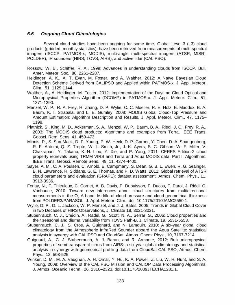
133
6.6 Ongoing Cloud Climatologies
Several cloud studies have been ongoing for some time. Global Level-3 (L3) cloud products (gridded, monthly statistics), have been retrieved from measurements of multi-spectral imagers (ISCCP, PATMOS-x, MODIS), multi-angle multi-spectral imagers (ATSR, MISR], POLDER), IR sounders (HIRS, TOVS, AIRS), and active lidar (CALIPSO).
Rossow, W. B., Schiffer, R. A., 1999: Advances in understanding clouds from ISCCP, Bull.
Amer. Meteor. Soc., 80, 2261-2287. Heidinger, A. K., A. T. Evan, M. Foster, and A. Walther, 2012: A Naïve Bayesian Cloud
Detection Scheme Derived from CALIPSO and Applied within PATMOS-x. J. Appl. Meteor. Clim., 51, 1129-1144.
Walther, A., A. Heidinger, M. Foster, 2012: Implementation of the Daytime Cloud Optical and Microphysical Properties Algorithm (DCOMP) in PATMOS-x. J. Appl. Meteor. Clim., 51, 1371-1390.
Menzel, W. P., R. A. Frey, H. Zhang, D. P. Wylie, C. C. Moeller, R. E. Holz, B. Maddux, B. A. Baum, K. I. Strabala, and L. E. Gumley, 2008: MODIS Global Cloud-Top Pressure and Amount Estimation: Algorithm Description and Results, J. Appl. Meteor. Clim., 47, 1175–1198.
Platnick, S., King, M. D., Ackerman, S. A., Menzel, W. P., Baum, B. A., Riedi, J. C., Frey, R. A., 2003: The MODIS cloud products: Algorithms and examples from Terra. IEEE Trans. Geosci. Rem. Sens, 41, 459-473.
Minnis, P., S. Sun-Mack, D. F. Young, P. W. Heck, D. P. Garber, Y. Chen, D. A. Spangenberg, R. F. Arduini, Q. Z. Trepte, W. L. Smith, Jr., J. K. Ayers, S. C. Gibson, W. F. Miller, V. Chakrapani, Y. Takano, K.-N. Liou, Y. Xie, and P. Yang, 2011: CERES Edition-2 cloud property retrievals using TRMM VIRS and Terra and Aqua MODIS data, Part I: Algorithms. IEEE Trans. Geosci. Remote Sens., 49, 11, 4374-4400.
Sayer, A. M., C. A. Poulsen, C. Arnold, E. Campmany, S. Dean, G. B. L. Ewen, R. G. Grainger, B. N. Lawrence, R. Siddans, G. E. Thomas, and P. D. Watts, 2011: Global retrieval of ATSR cloud parameters and evaluation (GRAPE): dataset assessment. Atmos. Chem. Phys., 11, 3913-3936.
Ferlay, N., F. Thieuleux, C. Cornet, A. B. Davis, P. Dubuisson, F. Ducos, F. Parol, J. Riédi, C. Vanbauce, 2010: Toward new inferences about cloud structures from multidirectional measurements in the O2 A band: Middle-of-cloud pressure and cloud geometrical thickness from POLDER3/PARASOL, J. Appl. Meteor. Clim., doi: 10.1175/2010JAMC2550.1.
Wylie, D. P., D. L. Jackson, W. P. Menzel, and J. J. Bates, 2005: Trends in Global Cloud Cover in two Decades of HIRS Observations, J. Climate 18, 3021-3031.
Stubenrauch, C. J., Chédin, A., Rädel, G., Scott, N. A., Serrar, S., 2006: Cloud properties and their seasonal and diurnal variability from TOVS Path-B. J. Climate, 19, 5531-5553.
Stubenrauch. C. J., S. Cros. A. Guignard, and N. Lamquin, 2010: A six-year global cloud climatology from the Atmospheric InfraRed Sounder aboard the Aqua Satellite: statistical analysis in synergy with CALIPSO and CloudSat. Atmos. Chem. Phys., 10, 7197-7214.
Guignard, A., C. J. Stubenrauch, A. J. Baran, and R. Armante, 2012: Bulk microphysical properties of semi-transparent cirrus from AIRS: a six year global climatology and statistical analysis in synergy with geometrical profiling data from CloudSat-CALIPSO, Atmos, Chem. Phys., 12, 503-525.
Winker, D. M., M. A. Vaughan, A. H. Omar, Y. Hu, K. A. Powell, Z. Liu, W. H. Hunt, and S. A. Young, 2009: Overview of the CALIPSO Mission and CALIOP Data Processing Algorithms, J. Atmos. Oceanic Techn., 26, 2310–2323, doi:10.1175/2009JTECHA1281.1.

134
A few are summarized below. 6.6.1 ISCCP
The ISCCP algorithm is described by Rossow (1989, 1993), Rossow et al. (1989),
Seze and Rossow (1991), and Rossow and Garder (1993). Only two channels are used, the narrow band visible (0.6 micron) and the infrared window (11 micron). Each observed radiance value is compared against its corresponding Clear-Sky Composite value. Clouds are assumed to be detected only when they alter the radiances by more than the uncertainty in the clear values. In this way the "threshold" for cloud detection is the magnitude of the uncertainty in the clear radiance estimates. The ISCCP algorithm is based on the premise that the observed VIS and IR radiances are caused by only two types of conditions, 'cloudy' and 'clear', and that the ranges of radiances and their variability that are associated with these two conditions do not overlap. As a result, the algorithm is based upon thresholds, where a pixel is classified as "cloudy" only if at least one radiance value is distinct from the inferred "clear" value by an amount larger than the uncertainty in that "clear" value. The uncertainty can be caused both by measurement errors and by natural variability. This algorithm is constructed to be "cloud-conservative," minimizing false cloud detections but missing clouds that resemble clear conditions.
The ISCCP cloud-detection algorithm consists of five steps: (1) space contrast test on a single IR image; (2) time contrast test on three consecutive IR images at constant diurnal phase; (3) cumulation of space/time statistics for IR and VIS images; (4) construction of clear-sky composites for IR and VIS every 5 days at each diurnal phase and location; and (5) radiance threshold for IR and VIS for each pixel. ISCCP detects high clouds from (a) only
infrared 11 m window channel data where it misses some thin cirrus clouds because there is no correction for the transmission of terrestrial radiation through the clouds; and (b) infrared window data corrected for cloud semi-transparency using the solar reflection measurements at
0.6 m with a radiative transfer model. 6.6.2 CLAVR (PATMOS-X)
The NOAA Cloud and AVHRR algorithm uses all five channels of AVHRR (0.63, 0.86, 3.7, 11.0, 12.0 microns) to derive a global cloud mask (Stowe et al., 1991). It examines multispectral information, channel differences, and spatial differences and then employs a series of sequential decision tree tests. Cloud free, mixed (variable cloudy) and cloudy regions are identified for 2x2 global area coverage (GAC) pixel (4 km resolution) arrays. If all four pixels in the array fail all the cloud tests, then the array is labelled as cloud-free (0% cloudy); if all four pixels satisfy just one of the cloud tests, then the array is labelled as 100% cloudy. If 1 to 3 pixels satisfy a cloud test, then the array is labelled as mixed and assigned an arbitrary value of 50% cloudy. If all four pixels of a mixed or cloudy array satisfy a clear-restoral test (required for snow/ice, ocean specular reflection, and bright desert surfaces) then the pixel array is re-classified as "restored-clear" (0% cloudy). The set of cloud tests is subdivided into daytime ocean scenes, daytime land scenes, nighttime ocean scenes and nighttime land scenes.
Subsequent improvements to the CLAVR incorporated dynamic clear/cloud thresholds predicted from the angular pattern observed from the clear sky radiance statistics of the previous 9-day repeat cycle of the NOAA satellite for a mapped one degree equal area grid cell (Stowe et al., 1994). As a further modification, CLAVR included pixel by pixel classification

135
based upon different threshold tests to separate clear from cloud contaminated pixels, and to separate cloud contaminated pixels into partial and total (overcast) cover. Cloud contaminated pixels are radiatively "typed" as belonging to low stratus, thin cirrus, and deep convective cloud systems. A fourth type indicates all other clouds, including mixed level clouds. CLAVR has evolved to the PATMOS-X cloud data set (Heidinger et al. 2012) 6.6.3 HIRS CO2 slicing
CO2 slicing (Wylie et al., 1994) has been used to distinguish transmissive clouds from opaque clouds and clear sky using High resolution Infrared Radiation Sounder (HIRS) multispectral observations. With spectral radiances around the broad CO2 absorption band at 15 microns, clouds at various levels of the atmosphere can be detected. Radiances from near the centre of the absorption band are sensitive to only upper levels while radiances from the wings of the band (away from the band center) see successively lower levels of the atmosphere. The CO2 slicing algorithm determines both cloud top pressure and cloud amount from radiative transfer principles. It has been shown to be especially effective for detecting thin cirrus clouds that are often missed by simple infrared window and visible approaches. Difficulties arise when the spectral cloud forcing (clear minus cloudy radiance for a spectral band) is less than the instrument noise. The technique is described in more detail in Chapter 8.
A statistical summary of over 76 million cloud observations from HIRS from 1979 to 2001 is shown in Table 6.3. In Table 6.3a, high clouds above 440 hPa comprise 33% of the observations. 18% of the observations are of clouds between 440 hPa and 700 hPa. Low clouds below 700 hPa are found 24% of the time. Cloud free conditions are found 25% of the time. Cirrus and transmissive clouds (with effective emissivities less than 0.95) are found in 43% of our observations; they range from 100 to 800 hPa. The 13% transmissive observations below 440 hPa are most likely broken clouds. Clouds opaque to infrared radiation (with effective emissivities greater than 0.95) are found 32% of the time. Table 6.3b shows the same cloud statistics corrected for the fact that HIRS does not observe lower cloud layers where higher cloud layers are found. This random overlap assumption yields a better representation of lower cloud coverages. Cloud frequency statistics are reported both ways in the literature, with and without correction for high cloud blockage. Accounting for blockage by high clouds, low clouds are inferred to be observed in 49% of the observations. The global average cloud
effective emissivity (global average of N) is found to be 0.54; Warren et al. (1988) report a global cloud fraction of 0.61 from ground observations.
Figure 6.14 shows the geographical distribution of all clouds in the summer and winter seasons. The months of December, January, and February represent the boreal winter (austral summer) and the months of June, July, and August represent the boreal summer (austral winter). The seasonal summaries are compiled using a uniformly spaced grid of 2
o
latitude by 3o longitude. Each grid box for each season has at least 1000 observations. The
Inter-Tropical Convergence Zone (ITCZ) is readily discernible as the region of more frequent clouds; the mid-latitude storm belts are also evident. The ITCZ is seen to move north with the sun from boreal winter to summer. The subtropical high pressure systems are seen in the regions of less frequent cloud cover. Over the Indonesian region the ITCZ expands in latitudinal coverage from boreal winter to summer. In the central Pacific Ocean, the ITCZ shows both a southern and northern extension during the boreal winter months. In the southern hemisphere, the eastern Pacific Ocean off South America and the eastern Atlantic Ocean off Africa remain relatively free of clouds throughout the year. The southern hemispheric storm belt is evident throughout the year. In the northern hemisphere’s mid-

136
latitude storm belts, the frequency of clouds increases during the winter with the strengthening of the Aleutian Low in the northern Pacific Ocean and the Icelandic Low in the northern Atlantic Ocean. The North American cloud cover shows little seasonal change. Large convective development occurs during the austral summer (boreal winter) in South America and Africa, which is readily apparent in the increased detection of clouds.
Observations of clouds above 6 km (Figure 6.14) exhibit the same general geographical
patterns found for total clouds (Wylie and Menzel, 2007). They are most predominant in the tropical ITCZ and move with the seasons. During the boreal winter in a few areas such as Southern Brazil, Tropical South Africa and Indonesia, high clouds are found in more than 90% of the observations. Less frequent occurrence is found in the mid-latitude storm belts. Differences in observations of high clouds and observations of all clouds are evident in the subtropical highs over the extra-tropical oceans where marine stratus clouds are prevalent and higher clouds are far less frequent. This is evident along the west coasts of North and South America and Africa.
Figure 6.15 shows the frequency of cirrus detection in the HIRS cloud studies from 1979 to 2001. Globally averaged frequency of cloud detection (excluding the poles where cloud detection is less certain) has stayed relatively constant at 75%; there are seasonal fluctuations but no general trends. High clouds in the upper troposphere (above 6 km) show a small increasing trend of ~ 2% per decade. The geographical locations of the cloud cover changes are studied using the difference of the average of the 1990s of the HIRS record subtracted from the average of 1980s (see Figure 6.16). Overall, the decadal average cloud cover has not changed appreciably from the 1980s to the 1990s. Small increases occurred in the tropics, mainly in the Indonesian Islands. Small decreases occurred in the sub-tropics, the eastern Sahara and in the central Pacific Ocean from Hawaii westward. The decreasing trend in Antarctica is uncertain because cloud detection itself is very difficult in the cold temperatures of Antarctica. Increases of 10% in the last decade for clouds above 6 km altitude occurred in the western Pacific, Indonesia, and over Northern Australia. Other fairly large increases occurred in western North America, Europe, the Caribbean, Western South America, and the Southern Ocean north of Antarctica. Decreases in high clouds occurred mainly in the tropical South Pacific, Atlantic and Indian Oceans south of the ITCZ.
While jet aircraft have been suspected of increasing cirrus cloud cover from their contrails, these data do not reveal such a trend. Increases of high clouds seem to occur in areas of high air traffic, such as central and western North America and Europe, as well as areas of rare air traffic, such as the Southern Ocean around Antarctica. It appears that high cloud cover changes are mostly caused by larger weather systems. The most significant feature of these data may be that the globally averaged cloud cover has shown little change in spite of dramatic volcanic and El Nino events. Figure 6.17 shows that during the four El Nino events winter clouds moved from the western Pacific to the Central Pacific Ocean, but their global average in the tropics did not change. El Chichon and Pinitubo spewed volcanic ash into the stratosphere that took 1-2 years to fall out, but cloud cover was not affected significantly.
These cloud data show overall constancy, with a possible small increase in high clouds. The high thin clouds capture some of the earth’s infrared radiation similar to CO2 and thus they contribute to global warming in the same manner. Clouds do not appear to be mitigating global warming by increasing their reflection of incoming solar radiation; they are possibly enhancing it

137
with modest increase of thermally trapping high thin ice clouds. These cloud trends will be re-analyzed after recalibration has reduced sensor to sensor spectral response and calibration differences. 6.6.4 UT/LS Clouds
Stratospheric clouds are considered to be important in global energy studies. The stratosphere is very dry, unlike the troposphere, and thus it rarely allows clouds to form. Stratospheric clouds usually occur as a result of convective intrusions from the troposphere into the stratosphere. Although they cover small areas in the atmosphere, they play a vital role in energy exchange in the atmosphere and they impact climate trends. In the tropics, convection resulting in stratospheric clouds is acknowledged to make a significant contribution of water vapor into the lower stratosphere. Tropical stratospheric cloud patterns are often indicative of Walker circulation cells, which are caused by differences in heat distribution between ocean and land. Stratospheric clouds cause radiative cooling and act to reduce the terrestrial infrared contribution to the stratospheric heat budget. In addition, the introduction of water vapor into the stratosphere contributes to the destruction of ozone.
High-resolution Infrared Radiation Sounder (HIRS) have been used to infer the presence of upper tropospheric and lower stratospheric (UT/LS) clouds and to track the trends in their occurrence in the mid-latitudes and tropics (Kolat et al. 2013). The HIRS has flown on sixteen satellites from TIROS-N through NOAA-19 and Metop-A and -B. Over this more than 30-year period, HIRS data have provided morning and afternoon coverage as well as overlapping coverage between platforms as new sensors are brought on-line. The approach is based on detection of the stratospheric lapse rate in the presence of high opaque clouds that fill the sensor field of view: a lower stratospheric or upper tropospheric cloud is inferred when a more absorbing spectral band sensitive to CO2 (HIRS band 5 at 14.0 µm) in the atmosphere produces a brightness temperature (BT) warmer than a less absorbing spectral band (HIRS band 7 at 13.3 µm). This is an indication of measurements from the stratosphere in the more absorbing spectral band wherein the lapse rate is positive; the opposite occurs in the troposphere wherein the lapse rate is normally negative.
HIRS data from 1987 to the present have been processed to investigate the UT/LS cloud trends. Most UT/LS clouds are found in the Inter-tropical Convergence Zone (ITCZ) as evidenced in Figure 6.18. Figure 6.19.a shows the fraction of observations for each month for each HIRS finding UT/LS clouds over the western Pacific (20S to 40N latitude; 45 to 180 longitude) from Jan 1987 to Dec 2011; percentage values range between 0.8 and 2.6%. Sensor to sensor consistency is reasonable; some differences are expected due to the orbit drift. Figure 6.19.b shows the average for each month. The seasonal differences with minima in the Dec-Jan-Feb and maxima in Jun-Jul-Aug are evident; a shift of about 0.7% is noticeable every year. The UT/LS cloud detection maxima in the ITCZ from 1990 until 1996 decrease from 2.5 to 2.0%, a brief period of increase through the El Niño event of 1998 restores the maxima at 2.4% in 2001, and thereafter a gradual decrease settles at 1.9% in 2011.
Figure 6.20 shows a companion plot of the fraction of HIRS observations finding UT/LS clouds in the eastern Pacific (20S to 40N latitude, 180 to 270 longitude) from Jan 1987 to Dec 2011. UT/LS clouds are found in 0.3 to 1.9 % for the eastern Pacific (Figure 6.20.a), down from the 1.0 to 3.0 % for the western Pacific (Figure 6.19.b). The seasonal cycle shows a minimum early in the year increasing to a maximum late in the year for both western and eastern Pacific, except in 1997 the year of the last major El Niño event. As noted in the study of Wylie and

138
Menzel (2008), the UT/LS detection in the western Pacific decreased while it increased more than usual in the eastern Pacific. Large increases from Feb to Oct are also evident in the eastern Pacific in the other El Niño years of 1986, 1991, 1994, and 2002; but 1997 stands out as the year of the largest increase.
The monthly Sea Surface Temperature (SST) records (Reynolds et al. 2002) in the Niño 3.4 region (5S to 5N latitude, 190 to 240 longitude) from Jan 1987 to Dec 2011 are shown in Figure 6.20b. The El Niño year of 1997 stands out with the Niño 3.4 SST maximum near 29 C and a maximum occurrence of eastern Pacific ITCZ UT/LS clouds near 1.4%. Moreover, at first glance it appears that the monthly eastern Pacific ITCZ UT/LS clouds for these twenty years are increasing when monthly Niño 3.4 SSTs are increasing and vice versa. A correlation coefficient of 0.61 is found for these monthly Niño 3.4 SSTs and eastern Pacific UT/LS cloud frequencies. Solomon et al. (2010) correlated stratospheric water vapor trends with the sea surface temperature over the western Pacific (the warm pool between 10S to 10N latitude 137 to 171 longitude); they found similar trends in the two citing the importance of stratospheric water vapor on decadel rates of warming as well as the need for further observations.
6.6.5 Comparison of Cloud Amount in Global Cloud Climatologies The GEWEX Data and Assessment Panel has compared available, global, long-term cloud data products with the International Satellite Cloud Climatology Project (ISCCP, Rossow and Schiffer 1999), which is the GEWEX cloud product and has been available since the 1980’s. The ISCCP cloud products were designed to characterize essential cloud properties and their variation on all key time scales to elucidate cloud dynamical processes and cloud radiative effects. The focus of the assessment was on the comparison of global climatological averages as well as their regional, seasonal and inter-annual variations derived from Level-3 (L3) cloud products (gridded monthly statistics). The presentations and discussions during four international workshops led to the current GEWEX Cloud Assessment database, including monthly averages, a measure of synoptic variability as well as histograms at a spatial resolution of 1° latitude x 1° longitude. It was created in a common netCDF format by the participating teams and is available at the GEWEX Cloud Assessment website: http://climserv.ipsl.polytechnique.fr/gewexca/, together with a detailed report (Stubenrauch et al. 2012). Cloud amount (CA), also often referred to as cloud cover, is the ratio between the number of samples that contain clouds and the number of all measurement samples. One expects an increase in CA by decreasing the spatial resolution (with the same detection sensitivity), especially in the case of low-level clouds which appear to be broken and more variable at smaller scales than upper-level clouds. However, the total cloud amount determined by a particular instrument also depends on the sensitivity of its measurements to the presence of clouds. The following has been concluded. * Global total cloud amount (see Figure 6.21) is about 0.68 (±0.03) when considering clouds with optical depth > 0.1. This value increases to about 0.73 when including sub-visible cirrus (CALIPSO-ST) and decreases to about 0.56 for clouds with optical depth > 2 (POLDER). * The average global inter-annual variability in CA is about 0.03, about ten times smaller than the typical day-to-day variability over the globe. * According to most datasets, oceans have about 0.10 to 0.15 more cloud than land. * The latitudinal variation in CA (not shown) of all datasets agrees well indicating subtropical subsidence regions with about 0.10 and 0.15 less cloudiness than the global mean

139
at around 20S and 20S respectively and the storm regions in the Southern Hemisphere (SH) midlatitudes with 0.15 to 0.25 more cloudiness than the global mean at around 60S. * The global spread in CA of these six datasets corresponds to only 0.08; however, locally, uncertainties in detecting clouds within the datasets may reach 0.4 over deserts and mountains. Another feature is the InterTropical Convergence Zone (ITCZ) where different sensitivities to thin cirrus may lead to a spread of about 0.15 in CA. The subtraction of the global annual means of the considered datasets leads to slightly improved uncertainty patterns in CA, emphasizing the good agreement for latitudinal variation. * Most datasets also agree on the magnitude of the seasonal cycle. In general, the seasonal variations are smaller than the latitudinal variations, except for the transition of the ITCZ towards the summer hemisphere, which produces a change of about 0.30 over land in the latitude band 0°-30S (Stubenrauch et al. 2012). Over ocean in the NH midlatitudes the seasonal change is about 0.15, with a minimum of cloudiness in late summer, whereas in the SH midlatitudes, it is negligible. References
Ackerman S. A., K. I. Strabala, W. P Menzel, R. E. Frey, C. C. Moeller, and L. E. Gumley,
1998: Discriminating clear sky from clouds with MODIS, J. Geophys. Res., 103, pp. 32141-32157.
Ackerman, S. A., 1996: Global satellite observations of negative brightness temperature differences between 11 and 6.7 um. J. Atmos. Sci., 53, 2803–2812.
Ackerman, S. A., R. E. Holz, R. Frey, E. W. Eloranta, B. C. Maddux, and M. McGill, 2008: Cloud detection with MODIS. Part II: Validation, J. Atmos. Oceanic Tech., 25, 1073-1086.
Baum B. A., D. P. Kratz, P. Yang, S. Ou, Y. X. Hu, P. F. Soulen, and S. C. Tsay, 2000: Remote sensing of cloud properties using MODIS Airborne Simulator imagery during
SUCCESS. I. Data and models, J. Geophys. Res., 105, pp. 11,767-11,780 Baum, B. A., W. P. Menzel, R. A. Frey, D. C. Tobin, R. E. Holz, S. A. Ackerman, A. K.
Heidinger, and P. Yang, 2012: MODIS Cloud Top Property Refinements for Collection 6,
Jour. Appl. Meteor. Clim., 51, No. 6, 1145-1163. Derber, J. C., D. F. Parrish, and S. J. Lord, 1991: The new global operational analysis system
at the National Meteorological Center, Weather Forecasting. 6, pp. 538-547 Frey, R. A., S. A. Ackerman, Y. Liu, K. I. Strabala, H. Zhang, J. R. Key, and X. Wang, 2008:
Cloud detection with MODIS. Part I: Improvements in the MODIS cloud mask for Collection
5, J. Atmos. Oceanic Tech., 25, 1057-1072. Holz, R. E., S. A. Ackerman, F. W. Nagle, R. Frey, S. Dutcher, R. E. Kuehn, M. Vaughan, and
B. A. Baum, 2008: Global MODIS cloud detection and height evaluation using CALIOP. J.
Geophys. Res., 113, D00A19, doi:10.1029/2008JD009837. King, M. D., W. P. Menzel, Y. J. Kaufman, D. Tanré, B. C. Gao, S. Platnick, S. A. Ackerman,
L. A. Remer, R. Pincus, and P. A. Hubanks, 2003: Cloud, Aerosol and Water Vapor
Properties from MODIS, IEEE Trans. Geosci. Remote Sens., 41, pp. 442-458 King, M. D., S. Platnick, W. P. Menzel, S. A. Ackerman, and P. A. Hubanks, 2012: Spatial and
Temporal Distribution of Clouds Observed by MODIS onboard the Terra and Aqua Satellites, accepted by IEEE Trans. Geosci. Remote Sens.
Kolat, U., W. P., E. Olson, and R. A. Frey, 2013: Very High Cloud Detection in More than Two Decades of HIRS Data, accepted by Journal of Geophysical Research.
Menzel W. P., D. P. Wylie, and K. I. Strabala, 1992: Seasonal and diurnal changes in cirrus
clouds as seen in four years of observations with the VAS, J. Appl. Meteor., 31, 370-385

140
Menzel W. P. and J. F. W. Purdom, 1994: Introducing GOES-I: The first of a new generation of
Geostationary Operational environmental Satellites. Bull. Amer. Meteor. Soc., Vol. 75, No. 5, pp. 757-781
Moeller, C. C., H. E. Revercomb, S. A. Ackerman, W. P. Menzel, and R. O. Knuteson, 2003: Evaluation of MODIS thermal IR band L1B radiances during SAFARI 2000. J. Geophys.
Res., 108, D13, 8494. Platnick S, M. D. King, S. A. Ackerman, W. P. Menzel, B. A. Baum, J. C. Riédi, R. A. Frey,
2003: The MODIS cloud products: algorithms and examples from Terra. IEEE Trans.
Geosci. Remote Sens., 41, pp. 459-473 Reynolds W. R., T. M. Smith, 1994: Improved global sea surface temperature analyses using
optimum interpolation. J. Climate, 7, 929-948 Reynolds, R. W., N. A. Rayner, T. M. Smith, D. C. Stokes, and W. Wang, 2002: An improved in
situ and satellite SST analysis for climate, J. Clim., 15, 1609–1625. Schmetz, J., S. A. Tjemkes, M. Gube, and L. van de Berg, 1997: Monitoring deep convection
and convective overshooting with Meteosat, J. Adv. Space Res., 10, 433–441. Seemann, S. W., E. E. Borbas, R. O. Knuteson, G. R. Stephenson, H.-L. Huang, 2008:
Development of a global infrared land surface emissivity database for application to clear sky sounding retrievals from multispectral satellite radiance measurements. J. Appl. Meteor.
Clim., 47, 108–123. Soden, B. J., and F. B. Bretherton, 1993: Upper tropospheric relative humidity from the GOES
6.7 µm channel: Method and climatology for July 1987. J. Geophysical Research, 98, 16669–16688.
Solomon, S., K. H. Rosenlof, R. W. Portmann, J. S. Daniel, S. M. Davis, T. J. Sanford, and G.-K. Plattner, 2010: Contributions of stratospheric water vapor to decadal changes in the rate
of global warming. Science, 327, 1219–1223. Strabala K. I., S.A. Ackerman, and W. P. Menzel, 1994: Cloud properties inferred from 8-12 µm
data, J. Appl. Meteorol., 33, pp. 212-229 Stubenrauch, C., 2006: Clouds, Chapter 6 in Observed Global Climate of Landolt-Börnstein
New Series III/XX. Stubenrauch, C. J., W. B. Rossow, S. Kinne and GEWEX Cloud Assessment Team, 2012:
Assessment of Global Cloud Datasets from Satellites, A Project of the World Climate Research Programme Global Energy and Water Cycle Experiment (GEWEX) Radiation Panel, WCRP report, 180 pp., in revision, available at : http://climserv.ipsl.polytechnique.fr/gewexca/.
Stubenrauch, C. J., W. B. Rossow, S. Kinne, S. Ackerman, G. Cesana, H. Chepfer, L. Di Girolamo, B. Getzewich, A. Guignard, A. Heidinger, B. Maddux, W. P. Menzel, P. Minnis, C. Pearl, S. Platnick, C. Poulsen, J. Riedi, S. Sun-Mack, A. Walther, D. Winker, S. Zeng, G. Zhao, 2013: Assessment of Global Cloud Datasets from Satellites. Accepted by Bull Amer Met Soc.
Wylie D. P. and W. P Menzel, 1999: Eight years of global high cloud statistics using HIRS. J.
Clim., 12, 170-184 Wylie, D. P., and W. P. Menzel, 2007: Clouds: Are the shutters of the Earth changing? In Our
changing planet: The view from space. M. D. King, C. L. Parkinson, K. C. Partington, and R. G. Williams, Eds. New York, NY: Cambridge University Press, 10-14.

141
Table 6.1: Longwave and Shortwave Window Planck Radiances (mW/m2/ster/cm
-1) and
Brightness Temperatures (degrees K) as a function of Fractional Cloud Amount (for cloud of 220 K and surface of 300 K) using B(T) = (1-N)*B(Tsfc) + N*B(Tcld).
Cloud
Fraction N
Longwave Window
Rad Temp
Shortwave Window
Rad Temp
Tsw -Tlw
1.0
23.5
220
.005
220
0
.8
42.0
244
.114
267
23
.6
60.5
261
.223
280
19
.4
79.0
276
.332
289
13
.2
97.5
289
.441
295
6
.0
116.0
300
.550
300
0

142
Table 6.2: Emissivity estimates for different surface types
(3.5-3.9)
(10.3-11.3)
(11.5-12.5)
Rocks: Igneous Granite.h2 Andesite.h1 Basalt.h1 Sedimentary Limestone.h1 Sandstone.h1 Shale.h1 Metamorphic Marble.h2 Quartzite.h1 Schist.h3a Slate.h1a
.91
.96
.96
.89
.83
.86
.94
.78
.90
.89
.91
.90
.90
.94
.96
.97
.95
.97
.94
.95
.95
.95
.95
.97
.98
.98
.98
.98
.96
.97 Soils: Entisols (quartz-rich) Vertisols (high clay content) Aridisols (desert,fine quartz, clay, carbonate soil) Mollisols (black organic-rich)
.85
.87
.75
.83
.97
.97
.97
.97
.98
.98
.97
.98 Vegetation Lichens Green Foliage Beech Hickory Red Oak Conifer Indian Grass Senescent Foliage Sen Beech Sen Red Oak Sen Pine Sen Rye Grass
.95
.95
.95
.97
.98
.97
.75
.84
.96
.85
.97
.95
.98
.95
.98
.96
.82
.91
.98
.91
.98
.96
.98
.95
.98
.98
.85
.92
.98
.91 Decomposing Soil Litter Deciduous Coniferous
.92
.94
.96
.98
.96
.98 Seawater and Distilled
97
.99
.99
Ice Sea Ice smooth Sea Ice 100 grit
.96
.93
.98
.99
.97
.97 Water Coatings Foam Oil 42667 Soil Float
.97
.96
.97
.99
.96
.98
.99
.96
.98
(Estimates made from average reflectance values reported in Salisbury and D’Aria (1992, 1994)).

143
Table 6.3a: UW NOAA Pathfinder HIRS cloud reports by cloud height and density
from 1979-2001. N refers to effective emissivity, and refers to the corresponding visible optical depth. Over 76,000,000 HIRS observations from 9 NOAA satellites are included. Percentages of all observations are reported.
Cloud Density
Thin Thick Opaque All
Cloud Level
N < 0.5
vis< 1.4
0.5<N<0.95
1.4 <vis < 6
N > 0.95
vis > 6
High (<440 hPa) 15 % 15 % 3 % 33 % Mid (440-700 hPa) 5 % 7 % 6 % 18 % Low (>700 hPa) 1 % 23 % 24 % Total 20 % 23 % 32 % 75 %
Table 6.3b: Table 6.3a statistics which have been corrected for the number of times the middle and low layers were actually observed by HIRS using the random overlap assumption.
Cloud Density
Thin Thick Opaque All
Cloud Level
N < 0.5
vis< 1.4
0.5<N<0.95
1.4 <vis < 6
N > 0.95
vis > 6
High (<440 hPa) 15 % 15 % 3 % 33 % Mid (440-700 hPa) 7 % 10 % 9 % 26 % Low (>700 hPa) 2 % 47 % 49 % Total 20 % 23 % 32 % 75 %

144
Figure 6.1: Ratio of the radiances for the two window channels; solid curve is the theoretical cloud free curve and dashed curve is the linear variation with cloud amount.
Figure 6.2: High spectral resolution total transmittance spectra for a standard atmosphere from 8 to 13 microns.

145
Figure 6.3: Emissivity of various soil and vegetation types as a function of wavelength.
Figure 6.4: The dependence on PW of the brightness temperature difference between the various window channels. Observed AVHRR 11-12 micron (top panel) and collocated HIRS 8-11 micron (bottom panel) brightness temperature differences plotted versus global model (NMC) total column PW for January 1994 over clear ocean scenes.

146
Figure 6.5: Schematic diagram of the effects of different atmospheric constituents on the brightness temperature differences 11 minus 12 microns and 8.6 minus 11 microns.
Figure 6.6: Indices of refraction of ice and water across the window region (a) real part and (b) imaginary part (associated with absorption). Note the greater absorption of ice over water for wavelengths greater than 10.5 microns.
Figure 6.7: Scatter diagram of collocated HIRS 8-11 versus AVHRR 11-12 micron brightness temperature differences for January 1994 over clear ocean scenes. As moisture increases, the 11-12 micron brightness temperature difference increases while the 8.6-11 micron brightness temperature difference decreases.

147
Figure 6.8: Albedo variations for ice, snow, and vegetation from 0.5 to 3.5 microns. Vegetation shows a sharp increase above 0.72 microns. Snow/ice shows a sharp decrease above 1.4 microns.
Figure 6.9: Example of infrared histogram analysis technique using AVHRR data for 2.5 by 2.5 degree ocean region. The derived clear sky brightness temperature threshold is 284.6 K.
Figure 6.10: Spatial variability test from stratus clouds over South America as an example of the arches obtained for AVHRR 11 µm brightness temperatures (x-axis) when plotting local deviation from mean (y-axis).

148
Figure 6.11: (Left) False color image (R: band 1, G: band 6, and B: band 31, flipped). High ice clouds are pink or blue, low water-phase clouds are yellow, land is green, and water is dark blue. (Right) IR cloud phase with ice clouds (blue), water clouds (red), mixed phase clouds (green), and uncertain phase (yellow).
Figure 6.12: MODIS Cloud Top Pressures inferred from the CO2 slicing technique for 4 April 2003. Mid-latitude cloud bands are clearly evident.

149
c
Figure 6.13: Detection of clouds in the upper troposphere/lower stratosphere (UT/LS) for a MODIS granule at 0800UTC on 28 August, 2006, over the Indian Ocean. (a) Brightness temperatures (K) for MODIS band 36 (14.2 µm), (b) 1-km pixels identified with the UT/LS cloud test are painted in red. (c) MODIS brightness temperature differences BTD[13.9-13.3 µm] are shown as a function of the difference between the CALIOP cloud-top height (CTH) and the tropopause height for August 2006. The tropopause height is determined from the temperature profiles in the GDAS model at the closest time and location to the MODIS data. The collocated data are from 60˚S-60˚N for both daytime/nighttime conditions over all surfaces, but are filtered for single-layered, overcast clouds. The colors are in log10 scale.

150
Figure 6.14: The frequency of all clouds and high clouds above 440 hPa from 1979 to 2001 found in HIRS data during winter (December, January, February) and summer (June, July, August).
Figure 6.15: The global frequency of all and high (above 6 km) cloud detection in a HIRS FOV since 1979 (excluding the poles where cloud detection is less certain). Major climatic events are also indicated. (a)

151
(b)
Figure 6.16: The geographical locations of changes in (a) All Cloud and (b) High Cloud frequency of detection from the 1980s to the 1990s.

152
(a)
(b)
Figure 6.17: High cloud (above 6 km) frequency of detection (a) during El Nino years compared with (b) all the other years during northern hemisphere winters (December, January, and February) during the 1980s to the 1990s.
Figure 6.18: Geographical distribution of the fraction of HIRS FOVs indicating the presence of UT/LS clouds for the CO2 test when BT(14.0 µm) > BT(13.3 µm) using NOAA-14 HIRS data for July 2001.

153
(a)
(b)
Figure 6.19: (a) Individual monthly UT/LS cloud fraction detected by each HIRS over the ITCZ (20S to 40N latitude; 45 to180 longitude) from Jan 1987 to Dec 2011. The number indicates the NOAA satellite (e.g. 0 for NOAA-10, 1 for NOAA-11, and so on) and the color indicates the orbit (red for descending morning and black for ascending afternoon). (b) Average monthly UT/LS cloud fraction detected by all HIRS on NOAA-10 through NOAA-19 over the ITCZ from Jan 1987 to Dec 2011.
x

154
(a)
1990 1995 2000 2005 20100
0.005
0.01
0.015
(b)
1990 1995 2000 2005 201024
25
26
27
28
29
30
SS
T (
C)
Figure 6.20: (a) Average monthly UT/LS cloud fraction detected by all HIRS on NOAA-10 through NOAA-19 over the eastern Pacific region (20S to 40N latitude, 180 to 270 longitude) of the ITCZ from Jan 1987 to Dec 2011. (b) Niño 3.4 (5S to 5N latitude, 190 to 240 longitude) Sea Surface Temperature (SST) from Jan 1987 to Dec 2011.

155
Figure 6.21: Global averages of total cloud amount (CA), as well as fraction of high-level, mid-level and low-level cloud amount relative to total cloud amount (CAHR + CAMR + CALR = 1) and global averages of effective cloud amount (cloud amount weighted by cloud emissivity) of high-level clouds (CAEH), of mid-level clouds (CAEM) and of low-level clouds (CAEL). Statistics are averaged over daytime measurements.

156
CHAPTER 7
SURFACE TEMPERATURE 7.1 Sea Surface Temperature Determination
Much of what has been presented so far has assumed knowledge of the surface temperature. In this section, techniques to determine surface temperature are discussed.
In the infrared, the emissivity of the earth's sea and land surface is near unity. As a result, in the absence of cloud or atmospheric attenuation, the brightness temperature observed with a space-borne window radiometer is nearly equal to surface skin temperature. However, cloud and water vapor absorption usually prohibit direct interpretation of the window channel data so that algorithms need to be applied to the data to alleviate the influence of clouds and water vapor absorption. The algorithms have evolved from the use of a single window channel on a polar orbiting satellite to the use of multispectral radiometer observations from both polar orbiting and geostationary satellites.
The earliest single channel approach involved a statistical histogram of brightness temperatures that was used to distinguish cloud free observations from cloud contaminated observations and to obtain sea surface temperature measurements. The following assumptions are implicit in the technique: (a) sea surface temperature is slowly varying, so cloud free infrared window measurements over the sea will be very repetitive and sea surface brightness temperature values will have a high frequency of occurrence, and (b) cloud contamination will produce lower brightness temperature values than sea surface and the cloud brightness temperatures will be highly variable over an area due to variations in cloud amount, opacity, and altitude.
A typical histogram is shown in Figure 7.1. Figure 7.1.a shows the normal distribution obtained when all measurements are cloud free and no SST gradient exists. Figure 7.1.b, on the other hand, illustrates the situation when more than half of the samples are cloud contaminated. Since the cloud-contaminated radiance temperatures are lower than the cloud free temperatures, they populate the left hand side of the histogram, but also distribute themselves normally. Only the warm side of the normal density curve formed by cloud free observations can be distinguished from the combined data in the histogram. Since the mean of the normal (Gaussian) density function (probability function) formed from clear observations is the most likely value of the SST, several schemes have been developed to infer the mean of a Gaussian probability function from knowledge of the standard deviation σ of the density function and knowledge of the inflection point on one side of the distribution.
7.1.1 Slope Method
The slope method assumes that the brightness temperature frequency distribution is a normal function of the form
f(T) = fs exp [ -(T - Ts)2/2σ
2 ]

157
where f is the frequency of occurrence, fs = f(Ts) is unknown, the standard deviation σ is assumed to be known from the characteristics of the measuring instrument, and the mean temperature Ts is the quantity to be determined. Since the standard deviation of a normal probability density function occurs at the inflection points on the curve, then
Ts = Tmax - σ where Tmax is the solution of
d2f/dT
2 = 0 ,
and σ is determined from the equation
σ = (σN2 + σE
2)½ ,
where σN and σE are the standard deviations, respectively, of the instrument noise and the expected variance of the SSTs. 7.1.2 Three Point Method
The three point method also assumes a normal probability function, and solves for Ts by selecting three points (Ti, fi), (Tj, fj), and (Tk, fk) on the warm side of the histogram as follows
fi = fs exp [-(Ti - Ts)2/2σ
2]
fj = fs exp [-(Tj - Ts)
2/2σ
2]
fk = fs exp [-(Tk - Ts)
2/2σ
2] .
These three equations contain three unknowns fs, σ, and Ts and can be solved by simple Gaussian elimination. Therefore
ln(fi /fj) = [(Ti2 - Tj
2)-2Ts (Ti - Tj)]/2σ
2 ,
ln(fi /fk) = [(Ti
2 - Tk
2)-2Ts (Ti - Tk)]/2σ
2 ,
or, finally,
Ti2 ln (fj/fk) - Tj
2 ln (fi/fk) + Tk
2 ln (fi/fj)
Ts = __________________________________________
2 [Ti ln (fj/fk) - Tj ln (fi/fk) + Tk ln (fi/fj)]
Since a single calculation of Ts can be influenced by noise and by the combination of
the three points being slightly non-Gaussian, repeated calculations of Ts are made from all possible unique combinations of three points on the warm side of the histogram. Thus, if there are n useful points on the warm side, then all possible i, j, k combinations are used to construct a second histogram, called the mean estimate histogram from which the most frequently occurring estimate is taken as the correct one.

158
7.1.3. Least Squares Method
Another solution is through a least squares fit of the normal distribution probability function to three or more points on the warm end of the observed frequency distribution. It follows from before that
ln (f(T)) = ln (fs) - Ts
2/2σ
2 + TsT/σ
2 - T
2/2σ
2
which has the form
ln (f(T)) = Ao + A1T + A2T2 ,
where
Ts = - A1/(2A2) , and
σ2 = - 1/(2A2) .
Thus, given several points (fi, Ti) on the cloud free portion of the histogram, one can solve for Ts and σ using the least squares solution.
7.2 Water Vapour Correction for SST Determinations
Corrrection for the effects of water vapor in the atmosphere is addressed here. The brightness temperature observed with a satellite radiometer can be equated to surface skin temperature after the effect of atmospheric water vapour absorption has been taken into account.
The surface temperature can be expressed in terms of the observed clear sky window
channel brightness temperature, Tb, and a water vapour correction, T;
TS = Tb + T .
The water vapour correction ranges from a few tenths of a degree Kelvin in very cold and dry atmospheres to nearly 10 K in very warm and moist atmospheres for 11 micron window observations. The corresponding corrections for the 3.7 micron window are about half as large. The water vapour correction is highly dependent on wavelength. To see why this is so, consider that at 3.7 micron, the Planck radiance varies with temperature to approximately the thirteenth power whereas at 11 micron the Planck radiance varies with temperature to approximately the fourth power. Inserting
Bλ(T) = T
nλ
Tbλnλ
~ λs(ps)Tsnλ
+ (1 - λs(ps))Tanλ
where λ(ps) is the atmospheric transmittance, Ts is the surface temperature, and Ta is the mean atmospheric temperature. Assuming representative values of 0.8, 300 K, and 270 K for
s, Ts, and Ta, respectively, one finds that at 3.7 micron where nλ = 13, the brightness temperature observed is 296.5 K as opposed to a value of 294.5 K observed at 11 micron where nλ = 4. Clearly for non-isothermal conditions and the same atmospheric transparency,

159
the water vapour correction does depend on wavelength. Figure 7.2a illustrates the water vapor corrections derived for the Nimbus-2 3.7 micron region due to the Planck radiance dependence discussed above. Note also the dependence of the water vapor correction on viewing angle.
The water vapour correction is best evaluated by observing the area of interest in multiple infrared window channels. In the atmospheric window regions, the absorption is weak, so that
w = e- kwu
~ 1 - kwu
where w denotes the window channel wavelength, and
dw = - kwdu
What little absorption exists is due to water vapour, therefore, u is a measure of precipitable water vapour. The RTE can be written in the window region
us
Iw = Bsw (1-kwus) + kw Bwdu o
us represents the total atmospheric column absorption path length due to water vapour, where s denotes surface. Defining an atmospheric mean Planck radiance
_ us us
Bw = Bwdu / du o o
then _
Iw = Bsw (1-kwus) + kwusBw . Since Bsw is close to both Iw and Bw, a first order Taylor expansion about the surface temperature Ts allows us to linearize the RTE with respect to temperature, so
_ Tbw = Ts (1-kwus) + kwusTw ,
_ where Tw is the mean atmospheric temperature corresponding to Bw. For two window channel wavelengths (11 and 12 micron) the following ratio can be determined.
_ Ts - Tbw1 kw1us(Ts - Tw1)
=
____________________
_ Ts - Tbw2 kw2us(Ts - Tw2)
Assuming that the mean atmospheric temperature measured in the one window region is comparable to that measured in the other, Tw1 ~ Tw2, we can simplify to

160
Ts - Tbw1 kw1
= _____
Ts - Tbw2 kw2
from which it follows that
kw1 Ts = Tbw1 +
[Tbw1 - Tbw2]
kw2 - kw1 This is the split window channel expression for the water vapour correction to the SST. The term split window is used to denote two neighbouring channels in a relatively transparent or window region of the spectrum; one channel for which the atmosphere is highly transparent and the other for which atmospheric water vapor partially absorbed the surface radiance to space. For three window channels (3.7, 11, and 12 µm) the analogous expression is
kw1 kw1 Ts = Tbw1 +
[Tbw1 - Tbw2] +
[Tbw1 - Tbw3]
2 (kw2-kw1) 2 (kw3-kw1)
Figure 7.2b provides a graphical representation of the multispectral window channel
water vapour correction algorithm. This linear extrapolation technique was first proposed by Anding and Kauth (1970) and initially tested by Prabhakara et al (1974). Accuracies of 1.0-1.5 C absolute and 0.5-1.0 C relative have been routinely achieved in the last few years.
Recently, a more sophisticated algorithm for atmospheric correction includes a
nonlinear term to account for absorption of water vapor in very wet atmospheres. Thus a quadratic term is added to the regression, as suggested by McMillin and Crosby (1984). The regression equation to correct for atmospheric absorption and re-emission has the form:
SST = A0 + A1*T11 + A2*T12 + A3*dT2
where dT = T11 – T12. It has been found that (A1 + A2) is close to one, with or without use of a quadratic term.
The instruments currently in use for the SST determinations include the AVHRR, MODIS, VIIRS, SEVIRI, and GOES Imager. The TIROS-N Advanced Very High Resolution Radiometer, Earh Observing System MODIS, and the Suomi NPP VIIRS are well-suited to measure surface temperatures since they detect radiation in the split window (water vapor absorption and window channels). However, observations from these polar orbiting satellites are not always timely (overpasses occur only two or four times per day over any given region). On the other hand, the SEVIRI and GOES Imager offer better than half hourly images at 4 km resolution (an order of magnitude more measurements of a given ocean surface). Thus, timely observations are available and the influence of clouds can often be alleviated by simply waiting for them to move out of the area of interest. Also, a given geographical region is always observed from the same viewing angle with the SEVIRI and GOES Imager so that relative variations of observed surface temperature variations rather than to variations in scan geometry. With multispectral window radiometer data routinely available from the

161
geostationary SEVIRI and GOES Imager, it is now possible to perform both precise water vapour correction and cloud filtering through quasi-continuous sampling with just one instrument. The SEVIRI and GOES cloud screening includes temporal continuity along with threshold tests with moisture corrected atmospheric infrared windows and visible reflectances. The following tests are used in the GOES SST algorithm for cloud detection.
T11 > 270 K ocean rarely frozen T11 > T12 + 4 K clouds affect moisture correction vis < 4% clouds reflect more than ocean sfc
T11 - T3.9 > 1.5 K subpixel clouds
T11 < 0.3 K SST over 1 hr small
-2 K < SST- guess < 5 K SST over days bounded GOES SSTs have been routinely generated every three hours in the vicinity of the continental USA since May 1997. The diurnal changes in the GOES SST are noticeable. As an example, Fig. 7.3a shows a three-day composite of the GOES SST around 1200 UTC (early morning), 20 to 22 May 1998, and Fig. 7.3b shows the difference eight hours later. The magnitude of the difference and the spatial distribution of the SST diurnal variation are remarkable. Variations as large as 3 K are found near the coast, where land contamination is a possible factor, and in regions where the surface wind is weak. Adequate validation and monitoring of such diurnal variations in surface skin temperatures is progressing; the implications are many. Climate analysis of SST is vulnerable to the variable sampling times of polar orbiting satellites. A sun-synchronous polar orbiting satellite passes a given geographical location at similar local times each day, nominally shortly after noon and midnight, to measure SST. In the presence of SST diurnal variation, if clouds at a location tend to appear at one of these times (say afternoon), the climatology can be biased towards the other time (nighttime SST). If clouds tend to appear at both times, the SST climatology must be estimated from other data. If the cloud diurnal variation varies seasonally, say clouds tend to appear in the afternoon in summer but not in winter, the SST can be biased towards the nighttime SST in summer but not in winter.
7.3 Accounting for Surface Emissivity in the Determination of SST
Since the sea surface emissivity is less than one, there are two effects that must be considered: (a) the atmospheric radiation reflects from the surface; and (b) the surface emission is reduced from that of a blackbody. The radiative transfer can be written ps
Iλ = ελ Bλ(Ts) λ(ps) + Bλ(T(p)) dλ(p) o
ps
+ (1-ελ) λ(ps) Bλ(T(p)) d↓λ(p)
o

162
where ↓λ(p) represents the transmittance down from the atmosphere to the surface. As before
in the derivation of the microwave RTE (in section 5.10), this can be derived in terms of the
transmittance up through the atmosphere to the top, λ(p). Then as before
o
Iλ = ελBλ(ps)λ(ps) + Bλ(T(p)) Fλ (p) dλ(p) ps
where
λ(ps) Fλ(p) = { 1 + (1 - ελ) [
]
2 } .
λ(p) Assuming that the atmosphere is a single layer whose temperature TA is the same for both upwelling radiance at the top of the atmosphere and the downwelling at the sea surface, then
Iλ = ελ Bλ(ps)λ(ps) + Bλ(TA) [1 - λ(ps) - (1-ελ)λ(ps)2 + (1-ελ)λ(ps)]
or
Iλ = ελ Bλ(ps)λ(ps) + Bλ(TA) [1 - ελ λ(ps) - λ(ps)2 + ελ λ(ps)
2] .
Note that as the atmospheric transmittance approaches unity, the atmospheric contribution expressed by the second term becomes zero.
Figure 7.4 shows a plot of the brightness temperature data observed from an interferometer at ship level and at 20 km altitude in the atmosphere, along with the split window brightness temperatures from the GOES imager. Figure 7.5 plots the associated radiances as a function of the correction term. The intercept of a regression line through these data is the Planck radiance corresponding to the sea surface temperature. In order to alleviate any scatter produced by the Planck radiance dependence on wavelength (or wavenumber), the observed radiances Iλ are converted to brightness temperature and then back to radiances for a reference wavelength λo. The emissivity values are taken from the literature (Masuda et al, 1988) and the transmittance values are computed from a line by line model in conjunction with an in situ radiosonde profile measurement. The retrieved value in this example yields 295.3 K within .2 K of in situ surface skin hat measurements (Smith et al, 1995). The correction from atmospheric reflection from the surface is comparable to the correction from the reduced surface emission.
7.4 Surface Emissivity
Thermal emission from from a land or sea surface is dependent on both the spectral emissivity, an intrinsic property of the surface determined by its composition and texture, and the surface temperature. Usually neither of these properties is well known a priori so that remote sensing of a surface has the problem of separating emissivity and temperature. Due to compositional and structural effects, the emission from a real solid may significantly deviate from that of a blackbody at the same temperature. To quantify these deviations, a measure of radiating efficiency called the directional spectral emissivity is defined as the ratio of the emitted thermal radiance of a body to the radiance expected from a blackbody at the same temperature. Thus at any given wavelength λ, emissivity is defined as the ratio of the actual emitted radiance, Rλ, to that from an ideal blackbody, Bλ,

163
λ (θ, Ф) = Rλ (θ, Ф, T) / Bλ (T) where sensor zenith θ and azimuth Ф must also be considered. Emissivity ranges between zero and one for all real substances. Figure 7.6 shows some of the surface emissivities at nadir viewing for some common surfaces (complementing those already shown in Figure 3.13). Water emissivity stays above 0.97 for all infrared spectral regions; land surface emissivities usually are above 0.90 but go as low as 0.75 near 4 microns for bare soil and desert surfaces.
7.5 Estimating Fire Size and Temperature
The most practical and economically feasible manner of monitoring the extent of burning associated with tropical deforestation and grassland management is through remote sensing. To date, many remote sensing methods have utilized multispectral data from the Multispectral Scanner (MSS) on Landsat-1, -2, ... , -5, the Thematic Mapper (TM) on Landsat-4 and -5, and the Advanced Very High Resolution Radiometer (AVHRR) on the NOAA polar orbiters (Tucker et al, 1984; Matson and Holben, 1987; Nelson et al, 1987; Malingreau and Tucker, 1988). Several techniques calculate vegetative indices in order to estimate deforestation areas (Justice et al, 1985; Malingreau et al, 1985; Townshend et al, 1987). However, the extent of deforestation is usually underestimated, mostly due to the inability to distinguish between primary and secondary growth (Malingreau and Tucker, 1988).
Another estimation of the rate of deforestation can be made by monitoring biomass burning. Matson and Dozier (1981) developed a technique utilizing the AVHRR 3.7 micron and 10.8 micron channels to detect subpixel resolution forest fires. The technique provides reasonable estimates of temperature and area of fires in those 1 km pixels that are not saturated (Matson and Holben, 1987). Unfortunately, many of the pixels are saturated. Moreover, it is difficult to monitor fire plume activity associated with these subpixel fires, since the NOAA polar orbiting satellite has only one day time pass over a given area. The geostationary GOES Imager and SEVIRI offer continuous viewing and less pixel saturation (because the pixel resolution is 3 km on SEVIRI, 4 km on GOES-8 Imager, or 16 km on GOES-7 VAS). Furthermore, the fire plumes can be tracked in time to determine their motion and extent. Thus the GOES satellite offers a unique ability to monitor diurnal variations in fire activity and transport of related aerosols.
The different brightness temperature responses in the two infrared window channels can be used to estimate the temperature of the target fire as well as the subpixel area it covers. Typically, the difference in brightness temperatures between the two infrared windows at 3.9 and 11.2 microns is due to reflected solar radiation, surface emissivity differences, and water vapour attenuation. This normally results in brightness temperature differences of 2 to 4 K. Larger differences occur when one part of a pixel is substantially warmer than the rest of the pixel. The hotter portion will contribute more radiance in shorter wavelengths than in the longer wavelengths. This can be seen in Figure 7.7 which depicts a portion of a line of VAS data over South America at 1831 UTC on 24 August 1988. Pixels a, b, and c represent areas where subpixel fires are burning. The largest temperature difference of about 15 K occurs at location b where the 11 micron brightness temperature value is 306.2 K and the 4 micron brightness temperature is 321.4 K. Warm areas surrounding these pixels are previously burned regions.

164
The fire extent and temperature within a field of view can be determined by considering the upwelling thermal radiance values obtained by the 4 and 11 µm channels (Matson and Dozier, 1981; Dozier, 1981). For a given channel, λ, the radiative transfer equation indicates 1
Rλ(T) = ελ Bλ(Ts) λ(s) + Bλ(T) dλ 0
When the GOES radiometer senses radiance from a pixel containing a fire of
blackbody temperature Tf occupying a portion p (between zero and one) of the pixel and a background of blackbody temperature Tb occupying the remainder of the pixel (1-p), the following equations represent the radiance sensed by the instrument at 4 and 11 µm.
R4(T4) = p R4(Tf) + ε4 (1-p) R4 (Tb) + (1-ε4) 4(s) R4(solar)
R11(T11) = p R11(Tf) + ε11 (1-p) R11(Tb) The observed short wave window radiance also contains contributions due to solar reflection that must be distinguished from the ground emitted radiances; solar reflection is estimated from differences in background temperatures in the 4 and 11 µm channels. Once Tb is estimated from nearby pixels, these two nonlinear equations can be solved for Tf and p. The solution to the set of equations can be found in several ways, one being to apply a globally convergent bisection technique followed by Newton's method.
Atmospheric corrections implicit in these equations are important. Burning or smoldering fires are usually covered by clouds and smoke containing organic particles of varying sizes and shapes, necessitating a correction to the transmittance. Most of the smoke is composed of water vapour, but there are other constituents as well (Andreae et al, 1988; Browell et al., 1988). The 11 µm channel is more affected by atmospheric water vapour than the 4 µm channel. With Nimbus-2 data, it was found that the water vapour correction for a moist atmosphere is approximately 4 K at 300 K for the 11 µm window and 2 K at 300 K for the 4 µm window (Smith et al, 1970). By calculating a linear regression relationship between the GOES visible brightness counts and GOES infrared window brightness temperature in a variety of haze conditions (approximately 50) and extrapolating to clear sky conditions, the Nimbus corrections were found to be appropriate for the GOES data studied (Prins and Menzel, 1994).
Emissivity investigations for vegetation similar to that found in the selva and cerrado suggest an emissivity for tropical rainforest of .96 in the 4 µm region and .97 in the 11 µm region, while the emissivity of dry grassland is .82 and .88 respectively (American Society of Photogrammetry, 1983).
The algorithm proceeds as follows. A fire is identified and a nearby fire free area is located. All observed brightness temperatures over the fire are adjusted for smoke attenuation; 2 K is added to the 4 µm brightness temperatures and 4 K is added to the 11 µm brightness temperatures. T4 and T11 represent the smoke corrected brightness temperatures over the fire for the two spectral bands. The background temperature, Tb11, is determined from the 11 micron brightness temperature in a nearby fire-free pixel (p=0) that is adjusted for surface emissivity. Subsequently, the shortwave window reflected radiance for this same fire-free pixel,

165
R4solar, is solved. The input parameters Tb11, T4, T11, and R4solar are now all in place; thus the equations can be solved for p and Tf (Prins and Menzel, 1994).
The process of fire identification is strongly dependent on image interpretation. A fire is suspected if the haze corrected 3.9 micron observed brightness temperature shows a 4 K increase over the 3.9 µm background temperature and the haze corrected 11.2 µm observed temperature displayed a 1 K increase above the 11.2 µm background temperature. Hot spots were not considered fires unless they were accompanied by some indication of a fire in the visible channel, such as a smoke plume. The temporal resolution of the GOES data is extremely useful in two ways. First, a hot spot is often evident in the infrared channels at a certain time period, but the corresponding visible channel showed little or no indication of a fire, possibly due to obscuration by a plume produced by a fire located upwind. A visible image a half hour earlier usually clarified whether a fire is located there. Second, it is difficult to distinguish regular clouds from plumes in a single image. By looping a series of half hourly visible images it is quite easy to identify the point sources of fires, since they remain at a constant location over time. In South America GOES-8 has been used to monitor trends in biomass burning and to catalogue the extent and transport of associated aerosols. The Automated Biomass Burning Algorithm (ABBA) developed by Prins and Menzel (1994) was used to monitor the 1995 biomass burning season in South America with GOES-8. Multi-spectral diurnal imagery (3-hourly) were collected from June through September to provide a clear picture of biomass burning activities throughout the burning season including estimates of sub-pixel size and mean temperature and information on smoke/aerosol transport. Figure 7.8.a shows the locations Locations of all GOES-8 ABBA detected fire pixels at 1445 UTC during the 1995 fire season (June-October 1995). Preliminary GOES-8 ABBA results obtained during the Smoke, Clouds, and Radiation (SCAR-B) experiment in Brazil (15 August - 15 September 1995) suggest that the peak burning time is in the middle of the afternoon (1800 UTC). Figure 7.8.b shows that the number of fires detected near 1800 UTC is 2 times greater than that observed 3 hours earlier or later and 8 times greater than that observed at 1200 UTC. The majority of the fire activity is concentrated along the perimeter of the Amazon in the Brazilian states of Para, Mato Grosso, Amazonas, and Rondonia. There is also considerable activity in Bolivia, Paraguay, and Northern Argentina. Compared to GOES-VAS, the improved spatial resolution available with GOES-8 provides much greater detail concerning fire activity and other surface features. During SCAR-B smoke was evident over a large portion of the continent east of the Andes Mountains in the GOES visible images. A large smoke pall covering over 4 million km
2 was
observed from 21 August through 11 September (an example is shown in Figure 7.9.a). Figure 7.9.b indicates that at the height of this burning period the smoke pall extended over nearly 7 million km
2. Transport over the Atlantic Ocean was observed on 13 days during the SCAR-B
field program. On at least two days a thin plume of smoke was tracked to the Prime Meridian.

166
Figure 7.1: Histograms of infrared window brightness temperature in cloud free and cloud contaminated conditions.
Figure 7.2a: Statistical relations of the water-vapour correction (y-axis) as a function of observed brightness temperature (x-axis) for two spectral channels and two viewing angles.
Figure 7.2b: Graphic representation of the linear relation between water vapour attenuation (x-axis) and brightness temperature (y-axis) for two different atmospheric conditions.

167
Figure 7.3a: Three-day composite of 1200 UTC GOES SST (early morning), May 20-22, 1998.
Figure 7.3b: Three-day composite of the difference in the GOES SST at 2000 UTC (afternoon) and 1200 UTC (early morning) for May 20-22, 1998. Differences greater than 3 K occur in clear skies in the tropics where the surface winds are less than 5 m/s (hence the ocean is relatively smooth).

168
Figure 7.4: Comparison of ocean brightness temperatures measured by a ship borne interferometer (AERI), by an interferometer (HIS) on an aircraft at 20 km altitude, and the geostationary sounder (GOES-8). Corrections for atmospheric absorption of moisture, non-unit emissivity of the sea surface, and reflection of the atmospheric radiance from the sea surface have not been made.
Figure 7.5: HIS and GOES radiance observations plotted in accordance with the radiative transfer equation including corrections for atmospheric moisture, non-unit emissivity of the sea surface, and reflection of the atmospheric radiance from the sea surface. Radiances are referenced to 880 cm-1. The intercept of the linear relationship for each data set represents a retrieved surface skin blackbody radiance from which the SST can be retrieved.
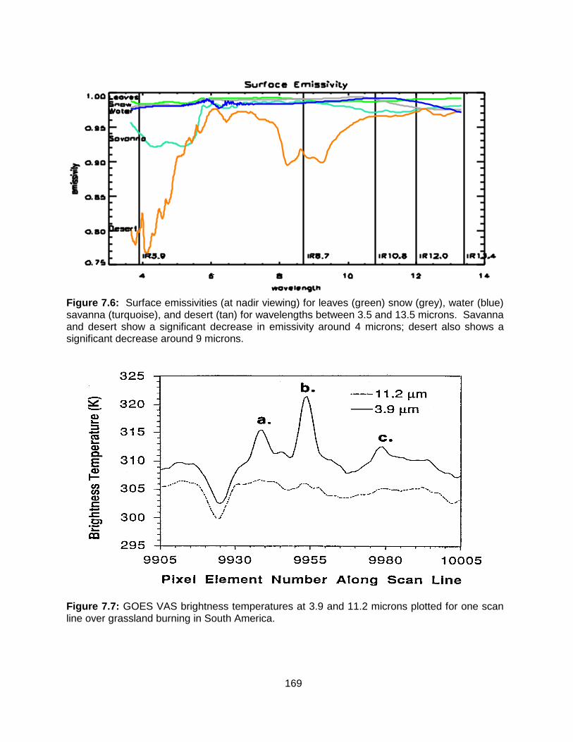
169
Figure 7.6: Surface emissivities (at nadir viewing) for leaves (green) snow (grey), water (blue) savanna (turquoise), and desert (tan) for wavelengths between 3.5 and 13.5 microns. Savanna and desert show a significant decrease in emissivity around 4 microns; desert also shows a significant decrease around 9 microns.
Figure 7.7: GOES VAS brightness temperatures at 3.9 and 11.2 microns plotted for one scan line over grassland burning in South America.
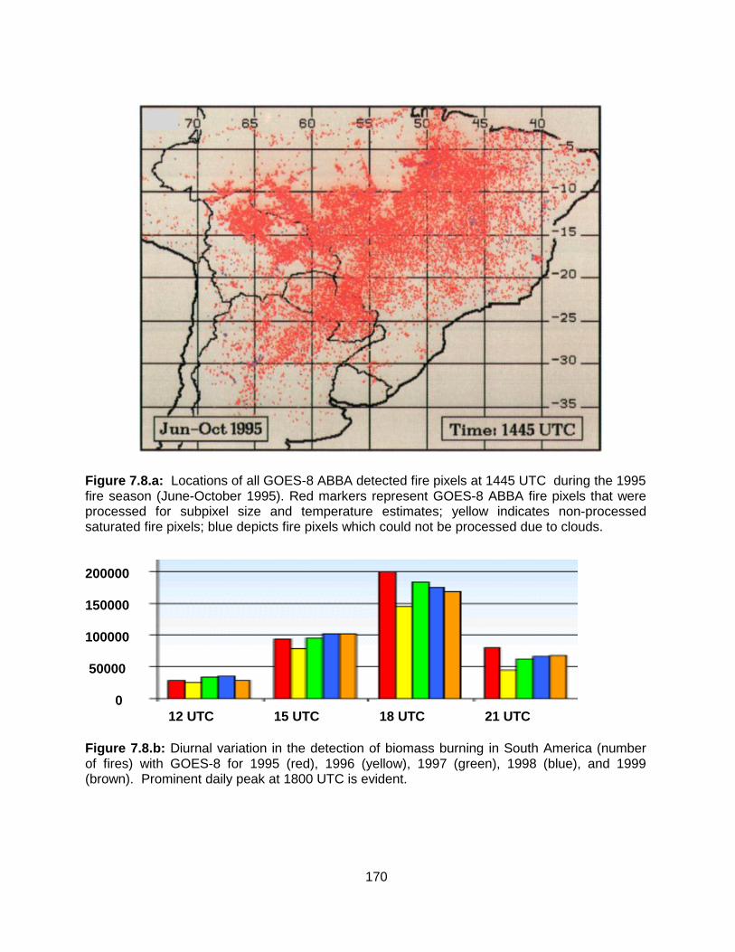
170
Figure 7.8.a: Locations of all GOES-8 ABBA detected fire pixels at 1445 UTC during the 1995 fire season (June-October 1995). Red markers represent GOES-8 ABBA fire pixels that were processed for subpixel size and temperature estimates; yellow indicates non-processed saturated fire pixels; blue depicts fire pixels which could not be processed due to clouds.
200000
150000
100000
50000
0
12 UTC 15 UTC 18 UTC 21 UTC
Figure 7.8.b: Diurnal variation in the detection of biomass burning in South America (number of fires) with GOES-8 for 1995 (red), 1996 (yellow), 1997 (green), 1998 (blue), and 1999 (brown). Prominent daily peak at 1800 UTC is evident.

171
Figure 7.9.a: GOES-8 visible image for August 28, 1995. Smoke is evident throughout the Amazon Basin covering over 6 million km2 and extending over to the Atlantic Ocean.
Figure 7.9.b: Estimates of daily smoke coverage over South America observed in GOES-8 visible imagery during August-September 1995.

172
CHAPTER 8
TECHNIQUES FOR DETERMINING ATMOSPHERIC PARAMETERS
8.1 Total Water Vapour Estimation
8.1.1 Split Window Method
The split window method can be used to specify total water vapour concentration from clear sky 11 and 12 micron brightness temperature measurements. In the derivation in section 7.2, it was shown that for a window channel Tbw - Ts
us =
. kw (Tatm - Ts)
Obviously, the accuracy of the determination of the total water vapour concentration depends upon the contrast between the surface temperature, Ts, and the effective temperature of the atmosphere, Tatm (when Ts = Tatm in an isothermal situation, the total precipitable water vapour concentration is indeterminate). The split window approximation allows us to write
kw2Tbw1 - kw1Tbw2 Ts =
,
kw2 - kw1 and if we express Tatm as proportional to Ts
Tatm = α Ts ,
then a solution for us follows: Tbw2 - Tbw1
us = _______________________________
(α-1)(kw2Tbw1 - kw1 Tbw2)
Tbw2 - Tbw1 =
___ .
β1Tbw1 - β2Tbw2
The coefficients β1 and β2 can be evaluated in a linear regression analysis from prescribed temperature and water vapour profile conditions coincident with in situ observations of us. The weakness of the method is due to the time and spatial variability of α and the insensitivity of a stable lower atmospheric state when Tbw1 ~ Tbw2 to the total precipitable water vapour concentration.
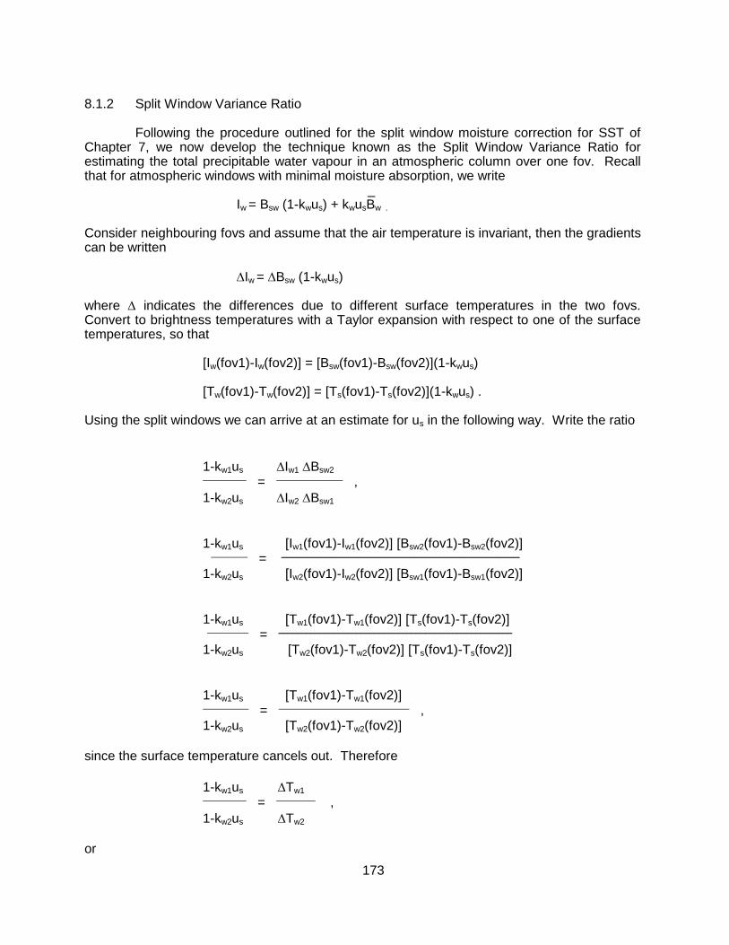
173
8.1.2 Split Window Variance Ratio
Following the procedure outlined for the split window moisture correction for SST of Chapter 7, we now develop the technique known as the Split Window Variance Ratio for estimating the total precipitable water vapour in an atmospheric column over one fov. Recall that for atmospheric windows with minimal moisture absorption, we write _
Iw = Bsw (1-kwus) + kwusBw .
Consider neighbouring fovs and assume that the air temperature is invariant, then the gradients can be written
Iw = Bsw (1-kwus) where indicates the differences due to different surface temperatures in the two fovs. Convert to brightness temperatures with a Taylor expansion with respect to one of the surface temperatures, so that
[Iw(fov1)-Iw(fov2)] = [Bsw(fov1)-Bsw(fov2)](1-kwus)
[Tw(fov1)-Tw(fov2)] = [Ts(fov1)-Ts(fov2)](1-kwus) . Using the split windows we can arrive at an estimate for us in the following way. Write the ratio
1-kw1us Iw1 Bsw2
=
,
1-kw2us Iw2 Bsw1
1-kw1us [Iw1(fov1)-Iw1(fov2)] [Bsw2(fov1)-Bsw2(fov2)]
=
____________________________________________________
1-kw2us [Iw2(fov1)-Iw2(fov2)] [Bsw1(fov1)-Bsw1(fov2)]
1-kw1us [Tw1(fov1)-Tw1(fov2)] [Ts(fov1)-Ts(fov2)]
=
___________________________________________________
1-kw2us [Tw2(fov1)-Tw2(fov2)] [Ts(fov1)-Ts(fov2)]
1-kw1us [Tw1(fov1)-Tw1(fov2)]
=
,
1-kw2us [Tw2(fov1)-Tw2(fov2)] since the surface temperature cancels out. Therefore
1-kw1us Tw1
=
,
1-kw2us Tw2 or

174
us = (1 - 12)/(kw1 - kw212), where 12 = Tw1/Tw2 represents the ratio of the deviations of the split window brightness temperatures. The deviation is often determined from the square root of the variance.
The assumption in this technique is that the difference in the brightness temperatures from one fov to the next is due only to the different surface temperatures. It is best applied to an instrument with relatively good spatial resolution, so that sufficient samples can be found in an area with small atmospheric variations and measurable surface variations in order to determine the variance of the brightness temperatures accurately. The technique was suggested by the work of Chesters et al (1983) and Kleespies and McMillin (1986); Jedlovec (1990) successfully applied it to aircraft data with 50 meter resolution to depict mesoscale moisture variations preceding thunderstorm development. 8.1.3 Perturbation of Split Window RTE
The total precipitable water vapour and the surface temperature can be determined from split window observations of a scene. Assuming that the temperature profile is well known for a given fov (so that T is zero), then the perturbation form of the radiative transfer equation (see section 5.8.2 of Chapter 5) can be written
Bs B ps B B
Tb = Ts [
/
] s + us
[
/
] dp Ts Tb o u p Tb
which reduces to the form
Tb = a Ts + b us . where a and b are calculable from the initial guess. The split window offers two equations and the two unknowns Ts and us are readily solved.
This technique is very dependent on the accurate absolute calibration of the instrument. 8.1.4 Microwave Split Window Estimation of Atmospheric Water Vapor and Liquid Water One can derive atmospheric water information from channels with frequencies below 40 GHz in the microwave spectrum. The 22.2 GHz channel has modest water vapor sensitivity and the 31.4 GHz channel has window characteristics; the two together are considered the microwave split window (analogous to the 11 and 12 micron infrared split window). Recalling the microwave form of the radiative transfer equation, o λ(p)
Tbλ = ελs T(ps) λ(ps) + T(p) Fλ(p)
d ln p ps ln p
where
λ(ps) Fλ(p) = { 1 + (1 - ελ) [
]2 } ,
λ(p)

175
one can write for the microwave windows
Tbλ = ελs Ts λs + Tatm [1-λs - (1-ελs) λs2 + (1-ελs) λs]
where Tatm represents an atmospheric mean temperature. Using λs ~ 1 - aλ and λs2 ~ 1 - 2aλ in
he window regions (where water absorption aλ is small), this reduces to
Tbλ = ελs Ts λs + Tatm [1 - ελs λs - λs2 + ελs λs
2] ,
Tbλ = ελs Ts (1 - aλ)+ Tatm [1 - ελs (1 - aλ)- (1 - 2aλ)+ ελs (1 - 2aλ)] , Tbλ = ελs Ts (1 - aλ)+ aλ Tatm [2 - ελs ] . But for low layers of moisture detected in the split window Ts ~ Tatm , so
Tbλ = ελs Ts + 2 aλ Ts [1 - ελs ] .
Writing λs = λs (liquid) λs (vapor) ~ [1-Q/Qo] [1- U/Uo], where Q is the total liquid concentration with respect to reference Qo and U is the total vapor concentration with respect to reference Uo, we get Tbλ = ελs Ts + 2 Ts [1 - ελs ] [Q/Qo + U/Uo]. If ελs and Ts are known, then measurements in the microwave split window offer solutions for Q and U (2 equations and 2 unknowns). Over oceans where the surface temperature and emissivity are reasonably well known and uniform, Q and U can be determined within 10%; however over land reliable solutions remain elusive. 8.2 Total Ozone Determination
Ozone is an important atmospheric constituent found in the atmosphere between 10 and 50 km above the earth's surface. Because it absorbs ultraviolet rays from the sun, ozone protects man from the harmful effects of ultraviolet radiation. Also, ozone is a prime source of thermal energy in the lower stratosphere and has been shown to be a useful tracer for stratospheric circulation. Prabhakara et al (1970) have exploited remote sensing of the total ozone using satellite infrared emission measurements and their studies reveal a strong correlation between the meridional gradient of total ozone and the wind velocity at tropopause levels. Shapiro et al (1982) have indicated a possibility to predict the position and intensity of jet streams using total ozone measured by satellite.
Recently, there has been increased interest in atmospheric ozone, due primarily to its role in complex middle atmospheric photochemistry and the critical ecological effect associated with ozone depletion induced by anthropogenic impacts and natural processes. By means of satellite observations, the evolution of the “ozone hole” and its interannual variability can be detected and even predicted. The main satellite instruments used for monitoring ozone are the Total Ozone Monitoring Sensor (TOMS) (Bowman and Krueger 1985; McPeters et al. 1996; McPeters et al. 1998) and the Solar Backscatter Ultraviolet (SBUV) spectrometer (Heath et al. 1975; Heath et al. 1978). In order to predict the evolution of ozone on time scales of a few days to a week, reliable global measurements of the three-dimensional distribution of ozone are needed. However, neither the TOMS nor the SBUV can provide measurements at night;

176
infrared (IR) radiance measurements as well as microwave limb sounders can. This section discusses infrared detection of ozone. 8.2.1 Total Ozone from Numerical Iteration
Ma et al (1983) suggested a method for obtaining total ozone with high spatial resolution from the TIROS-N/NOAA series of satellites. The ozone concentration is mapped with the 9.6 um ozone radiance observations by the High-resolution Infrared Radiation Sounder (HIRS). The meteorological inferences have a resolution of 75 km. The influence of clouds must be screened out to produce reliable ozone determinations.
Ozone concentration is related to radiance to space through the transmittance λ(p). As shown in the water vapour profile solution, using a first order Taylor expansion of Planck function in terms of temperature and integrating the RTE by parts, yields the expression
ps dp Tbλ - Tbλ
(n) = [λ(p) - λ
(n)(p)] Xλ(p)
_____
0 p where Tbλ is the measured brightness temperature, Tbλ
(n) is the brightness temperature
calculated for a nth estimate of the ozone profile, λ
(n)(p) is the corresponding transmittance
profile, and
Bλ(T) Bλ(T) T(p) Xλ (p) = [
| /
| ]
__________
T T lnp T=Tav T=Tbλ
Using the mathematical derivation used for water vapour retrieval, one can relate the brightness temperature measured by HIRS in the ozone 9.6 μm band to the ozone concentration, v(p):
ps v(p) dp Tbλ - Tbλ
(n) = ln
Zλ
(n)(p)
_____
o v(n)
(p) p where
Zλ
(n)(p) = λ
(n)(p) ln λ(n)(p) Xλ .
As suggested by Smith's generalized iteration solution, we assume that the correction to the ozone concentration v(p) - v
(n)(p) is independent of p, so that
v(p) Tbλ - Tbλ
(n)
= exp [
] = λ
(n)
v(n)
(p) ps dp Zλ
(n)(p)
____
o p

177
Consequently, for every pressure level, one can use this iterative procedure to estimate the true ozone concentration profile
v(n+1)
(pj) = v(n)
(pj) λ(n)
Convergence is achieved as soon as the difference between the measured ozone brightness temperature and that calculated is less than the measurement noise level (approximately 0.2 C). The first guess ozone profile is constructed using regression relations between the ozone concentration and the infrared brightness temperature observations of stratospheric carbon dioxide emission and the microwave brightness temperatures observations of stratospheric and tropospheric oxygen emission to space. Since ozone is a prime source of thermal energy in the low stratosphere and the upper troposphere, there is excellent correlation between the ozone concentration and the brightness temperatures observed in the HIRS carbon dioxide and MSU oxygen channels. Due to the fact that ozone and temperature sounding data yield good statistics only up to 10 mb (about 30 km), above 10 mb the ozone and temperature profiles are extrapolated using the lapse rate of USA standard ozone and temperature profiles between 10 mb and 0.1 mb (up to about 50 km). Above 50 km, the ozone contribution to the outgoing radiance is negligible.
The profile shape and the vertical position of the peak ozone mixing ratio
corresponding to the ozone guess profile is crucial to obtaining a satisfactory retrieval since only one ozone channel radiance in the 9.6 μm band is used. This is because the true ozone profile is assumed to have the same shape as the first guess. Therefore, to make the ozone guess profile sufficiently accurate in both shape and position of the ozone peak mixing ratio, adjustments to the vertical position and amplitude of the guess peak mixing ratio are made based on the difference between the observed brightness temperature and the calculated brightness temperature using the ozone guess profile. 8.2.2 Physical Retrieval of Total Ozone
Another approach to retrieving the total column ozone concentration is found in the perturbation form on the RTE. Assuming that the temperature and moisture profiles as well as the surface temperature are well known for a given FOV, then the perturbation form of the radiative transfer equation reduces to
ps T B B
Toz =
[
/
] dp
o p T Toz where Toz is the 9.6 μm brightness temperature. Finally, assume that the transmittance perturbation is dependent only on the uncertainty in the column of ozone density weighted path length v according to the relation
=
v
v Thus
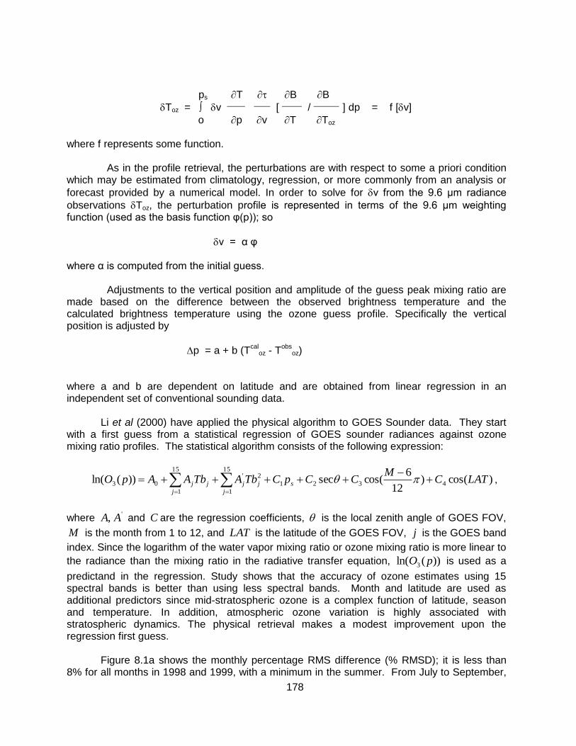
178
ps T B B
Toz = v
[
/
] dp = f [v]
o p v T Toz where f represents some function.
As in the profile retrieval, the perturbations are with respect to some a priori condition which may be estimated from climatology, regression, or more commonly from an analysis or
forecast provided by a numerical model. In order to solve for v from the 9.6 μm radiance
observations Toz, the perturbation profile is represented in terms of the 9.6 μm weighting function (used as the basis function φ(p)); so
v = α φ where α is computed from the initial guess.
Adjustments to the vertical position and amplitude of the guess peak mixing ratio are made based on the difference between the observed brightness temperature and the calculated brightness temperature using the ozone guess profile. Specifically the vertical position is adjusted by
p = a + b (Tcal
oz - Tobs
oz) where a and b are dependent on latitude and are obtained from linear regression in an independent set of conventional sounding data. Li et al (2000) have applied the physical algorithm to GOES Sounder data. They start with a first guess from a statistical regression of GOES sounder radiances against ozone mixing ratio profiles. The statistical algorithm consists of the following expression:
)cos()12
6cos(sec))(ln( 4321
15
1
15
1
2'
03 LATCM
CCpCTbATbAApO s
j j
jjjj
,
where ', AA and C are the regression coefficients, is the local zenith angle of GOES FOV,
M is the month from 1 to 12, and LAT is the latitude of the GOES FOV, j is the GOES band
index. Since the logarithm of the water vapor mixing ratio or ozone mixing ratio is more linear to
the radiance than the mixing ratio in the radiative transfer equation, ))(ln( 3 pO is used as a
predictand in the regression. Study shows that the accuracy of ozone estimates using 15 spectral bands is better than using less spectral bands. Month and latitude are used as additional predictors since mid-stratospheric ozone is a complex function of latitude, season and temperature. In addition, atmospheric ozone variation is highly associated with stratospheric dynamics. The physical retrieval makes a modest improvement upon the regression first guess.
Figure 8.1a shows the monthly percentage RMS difference (% RMSD); it is less than 8% for all months in 1998 and 1999, with a minimum in the summer. From July to September,

179
the % RMSD is less than 5%, indicating good agreement between GOES-8 ozone estimates and TOMS ozone measurements. Figure 8.1b shows a scatter plot of co-located GOES-8 ozone estimates and TOMS ozone measurements for June 1998 and January 1999. GOES-8 ozone estimates both in summer and in winter have good correlation with TOMS measurements. Although the ozone variation in winter is larger than in summer, the GOES-8 ozone estimates capture those variations well. To ascertain the longer-term quality and tendencies of the GOES-8 ozone estimates, single-site comparisons with ground-based Dobson-Brewer measurements were performed. Figure 8.1c shows the GOES-8 total ozone estimates for Bismarck, ND (46.77
oN, 100.75
oW) in 1998 along with the co-located TOMS and
ground-based ozone measurements. Ground-based ozone values are seen to vary from approximately 260 DU to 390 DU. Both TOMS and GOES ozone values match the range of ground-based ozone values well. However, GOES ozone estimates have larger bias and RMSD (-15.5 DU of bias and 25.4 DU of RMSD) than TOMS (-2 DU of bias and 17 DU of RMSD). 8.2.3 HIRS Operational Algorithm
An alternate approach for estimating total atmospheric column ozone follows the
NOAA operational HIRS algorithm. Total ozone is separated into upper and lower stratospheric contributions. Warm ozone in the upper stratosphere would be estimated directly from the model first guess; cold ozone in the lower stratosphere is estimated directly from its effect on the 9.6 μm channel radiance. Determination of lower stratospheric ozone requires an estimate of foreground temperature Tf and background temperature Tb. Tf is estimated from the model first guess 50 mb temperature. Tb is estimated from the infrared window brightness temperature in the absence of any ozone. The effects of upper stratospheric ozone are removed from the 9.6 μm radiance value by the following extrapolation
R`oz = [Roz - Au R(30mb)] / [1-Au] where from the model first guess we calculate
Au = 0.18 ESU(lat) ESU = EQ(lat) + SW EQ = 0.9 + 1.1 cos(lat) SW = DT [1 + DT (2+DT)] * [270 + lat] / 9000, DT = LR * WA / 40 LR = T(60mb) - T(100mb) -1, which is the tropopause lapse rate, and
WA = 2 * T(60mb) - T(30mb) - 205, which is the lower stratospheric temperature anomaly. Then

180
R’oz = ls Rb - (1 - ls) Rf
where ls is the transmittance through the lower stratosphere, Rb is the radiance from the
background, and Rf is the radiance from the foreground. Solving for ls yields the amount of total ozone by inverting Beer's law. 8.3 Determination of Cloud Height and Effective Emissivity
The determination of cloud heights is important for many meteorological applications,
especially the estimation of the pressure-altitude of winds obtained by tracing clouds from time sequenced satellite images. Several methods for determining cloud heights using satellite data have been developed over the years. One method (Fritz and Winston 1962) compares the infrared window channel brightness temperature with a vertical temperature profile in the area of interest to obtain the height of the cloud. This infrared window cloud height determination assumes the cloud is opaque and fills the satellite instruments field-of-view, and thus it works fine for dense stratoforms of cloud. However, it is inaccurate for semi-transparent cirrus clouds and small element cumulus clouds. A second method (Mosher 1976; Reynolds and Vonder Haar 1977) improves the infrared window channel estimate of cloud top height by allowing for fractional cloud cover and by estimating the cloud emissivity from visible reflectance data. Using a multiple scattering model, the visible brightness of the cloud is used to calculate the optical thickness, from which the infrared emissivity of the cloud can be computed. Although this bi-spectral method is an improvement over the first method, it is still inaccurate for semi-transparent cirrus clouds. A third method utilizes stereographic observations of clouds from two simultaneously scanning geosynchronous satellites (Hasler 1981). These stereo height measurements depend only on straightforward geometrical relationships and offer more reliable values than the previously discussed infrared-based methods. However, the stereo method is limited to the overlap region of the two satellites and to times when simultaneous measurements can be orchestrated.
The CO2 absorption method enables one to assign a quantitative cloud top pressure to a given cloud element using radiances from the CO2 spectral bands. Recalling that the radiance from a partly cloudy air column region by
Iλ = η Iλcd
+ (1-η) Iλcl
where η is the fractional cloud cover, Iλ
cd is the radiance from the cloud obscured field of view,
and Iλcl is the radiance from a clear field of view for a given spectral band λ. The cloud radiance
is given by
Iλcd
= ελ Iλbcd
+ (1-ελ) Iλcl
where ελ is the emissivity of the cloud, and Iλ
bcd is the radiance from a completely opaque cloud
(black cloud). Using the RTE, we can write

181
cl o Iλ = Bλ(T(ps)) λ(ps) + Bλ(T(p)) dλ ,
ps
bcd o Iλ = Bλ(T(pc)) λ(pc) + Bλ(T(p)) dλ .
pc where pc is the cloud top pressure. Integrating by parts and subtracting the two terms we get
cl bcd ps Iλ - Iλ = λ(p) dBλ pc
therefore
cl pc Iλ - Iλ = ηελ λ(p) dBλ ,
ps where ηελ is often called the effective cloud amount. The ratio of the deviations in cloud produced radiances and corresponding clear air radiances for two spectral channels, λ1 and λ2, viewing the same field of view can thus be written
cl pc Iλ1 - Iλ1 ελ1 λ1(p) dBλ1
ps
=
______________________
cl pc Iλ2 - Iλ2 ελ2 λ2(p) dBλ2
ps
If the wavelengths are chosen close enough together, then ελ1 = ελ2, and one has an expression by which the pressure of the cloud within the field of view (FOV) can be specified.
The left side can be determined from radiances observed by the sounder (HIRS and
the GOES Sounder) and clear air radiances calculated from a known temperature and moisture profile. Alternatively, the clear air radiances could be provided from spatial analyses of HIRS or GOES Sounder clear sky radiance observations. The right side is calculated from known temperature profile and the profiles of atmospheric transmittance for the spectral channels as a function of pc, the cloud top pressure. The optimum cloud top pressure is determined when the absolute difference [right (λ1,λ2,) - left (λ1,λ2,pc)] is a minimum.
These are two basic assumptions inherent in this method: (a) the cloud has infinitesimal thickness; and (b) the cloud emissivity is the same for the two spectral channels. The maximum possible error caused by assumption (a) is one-half the cloud thickness. Errors approaching one-half the cloud thickness occur for optically thin clouds (integrated emissivity roughly less than 0.6); for optically thick clouds (integrated emissivity roughly greater than 0.6) the error is small, typically one-fourth the cloud thickness or less. Errors due to assumption (b) can be minimized by utilizing spectrally close channels.

182
Once a cloud height has been determined, an effective cloud amount can be evaluated from the infrared window channel data using the relation
Iw - Iwcl
ηεw = __________________
Bw(T(pc)) - Iw
cl
where w represents the window channel wavelength, and Bw(T(pc)) is the window channel opaque cloud radiance.
Using the ratios of radiances of the three to four CO2 spectral channels on the polar or geostationary sounder, two to three separate cloud top pressures can be determined (for example 14.2/14.0 and 14.0/13.3). If (Iλ - Iλ
cl) is within the noise response of the instrument
(roughly 1 mW/m2/ster/cm
-1) the resulting pc is rejected. Using the infrared window and the two
cloud top pressures, two effective cloud amount determinations are made. To select the most representative cloud height pck, the algorithm checks the differences between the observed values of (Iλ - Iλ
cl) and those calculated from the radiative transfer equations for the two possible
cloud top pressures and effective cloud amounts,
pck [(I - I
cl)λ - ηεk λ dBλ] = Mλk .
ps
Pck is chosen when
Σ Mλk2
λ=1 is a minimum, where the sum is over the CO2 channels needed to derive the cloud top pressure values. Alternatively one can choose the cloud top pressure determined from the most opaque spectral channel pair (those with the highest weighting functions, as they will be most sensitive to the signal of the high cloud).
If neither ratio of radiances (14.2/14.0 or 14.0/13.3) can be reliably calculated because the cloud induced radiance difference (I - I
cl) is within the instrument noise level, then a cloud
top pressure is calculated directly from the sounder observed 11.2 μm infrared window channel brightness temperature and the temperature profile. In this way, all clouds can be assigned a cloud top pressure either by CO2 absorption or by infrared window calculations.
Menzel et al (1983) utilized the CO2 absorption method to make several comparisons
of cloud heights determined by different techniques; the comparisons were randomly made over several different cloud types including thin cirrus clouds. The CO2 heights were found to be reliable within about a 50 mb root mean square deviation of other available height determinations. The CO2 heights produced consistently good results over thin cirrus where the bi-spectral heights were inconsistent. This is demonstrated in Fig. 8.2, where bi-spectral and CO2 heights are plotted along a cirrus anvil blowing off the top of a thunderstorm at 1348 GMT 14 July 1982 over western Missouri and eastern Kansas. As one moves away from the dense cumulus clouds towards the thin cirrus, the CO2 absorption method maintains high altitudes while the bi-spectral method frequently underestimates the altitude by varying amounts depending on the thinness of the cirrus clouds.
The considerable advantage of the CO2 absorption method is that it is not dependent on the fractional cloud cover or the cloud emissivity (in fact the effective cloud amount is a by-product of the calculations).

183
8.4 Geopotential Height Determination
The geopotential Φ at any point in the atmosphere is defined as the work that must be done against the earth's gravitational field in order to raise a mass of 1 kg from sea level to that point. In other words, Φ is the gravitational potential for unit mass. The units of geopotential are 1 kg
-1 or m
2 s
-2. The force (in newtons) acting on 1 kg at height z above sea level is
numerically equal to g. The work (in joules) in raising 1 kg from z to z+dz is g dz; therefore,
dΦ = g dz = - α dp where α is the reciprocal of the density of air. The geopotential Φ(z) at height z is thus given by
z Φ(z) = g dz
o where the geopotential Φ(0) at sea level (z = 0) has, by convention, been taken as zero. It should be emphasized that the geopotential at a particular point in the atmosphere depends only on the height of that point and not on the path through which the unit mass is taken in reaching that point. The work done in taking a mass of 1 kg from point A with geopotential ΦA to point B with geopotential ΦB is ΦB - ΦA.
We can also define a quantity called the geopotential height Z as
Φ(z) 1 z Z =
=
g dz
go go o where go is the globally averaged acceleration due to gravity at the earth's surface (taken as 9.8 ms
-2). Geopotential height is used as the vertical coordinate in most atmospheric
applications in which energy plays an important role. It can be seen from Table 8.1 that the values of z and Z are almost the same in the lower atmosphere where go ~ g.
From the ideal gas law and the hydrostatic equation, we are able to write
dp pg
= -
_____
dz RT so that
p2 dp Φ2 - Φ1 = - R T
_____
p1 p or
R p1 dp Z2 - Z1 =
T
.
go p2 p
Therefore, having derived a temperature profile from sounding radiance measurements, it is possible to determine geopotential heights (or thicknesses). It is readily apparent that the thickness of the layer between any two pressure levels p2 and p1 is proportional to the mean temperature of the layer; as T increases the air between the two pressure levels expands so that the layer becomes thicker.

184
Geopotential heights and thicknesses are being processed routinely from GOES
soundings. An example comparison with conventional radiosonde and dropwindsonde determinations for 1982-83 are shown in Table 8.2. Most comparisons were made with the raobs at 1200 GMT wherever GOES soundings were sufficiently close in space and time (within approximately two hours and 100 km). Thickness derived from GOES temperature soundings showed a mean difference of only 10-30 meters when compared with raobs and 5-10 meters when compared with dropsondes.
Geopotential thickness are also routinely evaluated from the TIROS polar orbiters, but here the 850-500 and 850-200 hPa layers are estimated from a linear combination of the four MSU brightness temperature observations. Regression coefficients are determined from an analysis of radiosonde data. The 850-500 and 850-200 hPa thicknesses are useful for weather forecasting, since contour analyses of these quantities describe the direction and speed of the circulation at mid-tropospheric and jet stream levels, respectively. The accuracies of the MSU derived thicknesses are comparable to the accuracies experienced with the GOES derived heights and thicknesses. Figure 8.3 shows an example comparison of the NOAA-6 MSU estimates of the 850-500 and 850-200 hPa (mb) thickness patterns with those obtained from radiosonde observations. The patterns are very similar. 8.5 Microwave Estimation of Tropical Cyclone Intensity
It has been observed that the upper tropospheric temperature structure of tropical cyclones is characterized by a well-defined warm temperature anomaly at upper levels in well-developed storms. An intense tropical cyclone with an eye produced by subsidence within the upper tropospheric anticyclone develops a warm core due to adiabatic warming. One theory is the warm air produced by subsidence within the eye is entrained into the eye wall where strong upward motions transport this warmer air to high levels where it then diverges outward away from the eye region.
It has been shown to be possible to monitor the intensity of tropical cyclones as categorized by its surface central pressure and maximum sustained wind speed at the eye wall with satellite microwave observations. The relationship between surface pressure and the intensity of the warm core comes from the ideal gas law and the hydrostatic equation
dp g
= -
dz
p RT or
ps g zt dz ln [
] =
_____
pt R o T where ps is the surface pressure and pt and zt are the pressure and height of some level which is undisturbed by the tropical cyclone below. Thus, the surface pressure is inversely related to the temperature of the column of air above. Observations show that the transition between the lower level cyclone and upper level anti-cyclone occurs in the vicinity of 10 km. Applying the above equation at the eye and its environment we find

185
ps
eye g zt
ln (
) = ___
_______
pt R Tav
eye
and ps
env g zt
ln (
) = ___
________
pt R Tav
env
where Tav is the mean temperature of the column between the surface and the undisturbed pressure level. Combining these expressions we can write
gzt Taveye
- Tavenv
ps
eye = ps
env exp [ -
(
) ]
R Taveye
Tavenv
Using zt = 10 km and setting Tav
eye Tav
eye ~ (250 K)
2 then
ps
eye ~ ps
env exp [- 0.0055 Tav]
~ psenv
[1 - 0.0055 Tav] . Assuming ps
env ~ 1000 mb, then
ps
eye - 1000 = - 5.5 Tav
so that a 55 mb surface pressure depression is approximately associated with a 10 C contrast between the mean temperatures of the cyclone eye and its environment.
It has been found that the tropical cyclone warm core is usually strongest at about 250 hPa. In addition, the amplitude of the upper tropospheric temperature anomaly is well-correlated with the amplitude of the mean temperature of the tropospheric column below 10 km. Therefore, the deviation of the temperature field at 250 hPa provides a measure of the strength of the warm core, which then is correlated to storm surface intensity. Furthermore, a correlation should also exist for maximum surface winds as they are directly related to the pressure field (although not pure gradient winds because of frictional effects).
In the work of Velden et al (1984), T250 is compared to observed surface central pressure and maximum winds, where T250 is the gradient of the 250 hPa temperature field defined as the core temperature minus the average environmental temperature at a six degree radius from the storm core. Linear regression is used to find a best fit for the data. After studying over 50 cases, they found that the standard error of estimates for the central pressure and maximum wind are 6 hPa and 10 knots, respectively. Figure 8.4 shows these results. Figure 8.5 shows an example comparison of National Hurricane Centre (now called Tropical Prediction Center) versus satellite estimates of the central surface pressure and maximum sustained wind speed for the duration of Hurricane Barry. TOVS microwave intensity estimates continue to augment existing methods.

186
8.6 Satellite Measure of Atmospheric Stability
One measure of the thermodynamic stability of the atmosphere is the total-totals index
TT = T850 + TD850 - 2T500 where T850 and T500 are the temperatures at the 850 and 500 hPa levels, respectively, and TD850 is the 850 hPa level dew point. TT is traditionally estimated from radiosonde point values. For a warm moist atmosphere underlying cold mid-tropospheric air, TT is high (e.g., 50-60 K) and intense convection can be expected. There are two limitations of radiosonde derived TT: (a) the spacing of the data is too large to isolate local regions of probable convection; and (b) the data are not timely since they are available only twice per day.
If we define the dew point depression at 850 hPa, D850 = T850 - TD850 , then
TT = 2(T850 - T500) - D850 . Although point values of temperature and dew point cannot be observed by satellite, the layer quantities observed can be used to estimate the temperature lapse rate of the lower troposphere (T850 - T500) and the low level relative moisture concentration D850. Assuming a constant lapse rate of temperature between the 850 and 200 hPa pressure levels and also assuming that the dew point depression is proportional to the logarithm of relative humidity, it can be shown from the hydrostatic equation that
TT = 0.1489 ΔZ850-500 - 0.0546 ΔZ850-200 + 16.03 ln RH, where ΔZ is the geopotential thickness in metres and RH is the lower tropospheric relative humidity, both estimated from either TIROS or GOES radiance measurements as explained earlier.
Smith and Zhou (1982) reported several case studies using this approach. Figure 8.6 shows the total-totals stability index as observed by radiosondes and infrared from TOVS data on 31 March 1981. One can see the coarse spacing of the radiosonde observations (Figure 8.6.a). The analysis of satellite data possesses much more spatial detail since the spacing of the data is only 75 km (Figure 8.6.b). There is general agreement in the high total-totals over Illinois and Missouri, but also some areas of disagreement (e.g., Nebraska). In this case, the radiosonde data are not as coherent an indicator of the region of intense convection as are the satellite data.
Also shown on the satellite TT analysis are the streamlines of the wind observed at the surface. On this occasion, it appears that the unstable air observed along the Illinois-Iowa border at 1438 GMT was advected into central Wisconsin and supported the development of a tornadic storm at 2315 GMT.

187
Table 8.1: Values of the Geometric Height (z), Geopotential height (Z), and Acceleration Due to Gravity (g) at 40 Latitude
z(km)
Z(km)
g(ms-2)
0
0
9.802
1
1.000
9.798
10
9.9869
9,771
20
19.941
9.741
30
29.864
9.710
60
59.449
9.620
90
88.758
9.531
120
117.795
9.443
160
156.096
9.327
200
193.928
9.214
300
286.520
8.940
400
376.370
8.677
500
463.597
8.427
600
548.314
8.186

188
Table 8.2.a: Summary of Comparisons Between GOES(VAS) and Radiosonde Data For Bermuda, San Juan and West Palm Beach (1 August-30 November 1983)
Parameter
Mean
(VAS-RAOB)
Standard Deviation
Range
Number of
Cases Z850 (m)
7
10
-23 to 31
68
Z700
13
13
-21 to 36
67
Z500
18
19
-26 to 38
67
Z400
22
20
-37 to 66
65
Z300
30
27
-52 to 71
63
Z200
32
37
-63 to 110
62
Z500-850 (m)
12
15
-31 to 63
69
Z400-850
16
18
-42 to 50
67
Z300-850
23
26
-63 to 71
65
Z500-700
6
12
-28 to 52
68
Z400-700
10
16
-39 to 35
66
Z200-400
9
28
-78 to 60
63
Table 8.2.b: Summary of Comparisons Between GOES(VAS) and ODW For 14-15 and 15-16 September 1982 Parameter
Mean
(VAS-RAOB)
Standard Deviation
Range
Number of Cases
Z850 (m)
-6
23
-68 to 26
42
Z700
0
22
-58 to 41
42
Z500
1
24
-56 to 44
35
Z400
2
27
-54 to 47
24
Z400-850 (m)
11
17
-16 to 45
24
Z500-850
6
14
-18 to 43
35
Z400-700
4
14
-16 to 34
24

189
Percentage RMS difference between GOES-8 and TOMS ozone values
0
1
2
3
4
5
6
7
8
May-98 Jun-98 Jul-98 Aug-98 Sep-98 Oct-98 Nov-98 Dec-98 Jan-99 Feb-99 Mar-99 Apr-99 May-99 Jun-99 Jul-99 Aug-99 Sep-99
Month
%R
MS
D
Figure 8.1.a: The monthly % RMSD between the GOES-8 ozone estimates and the TOMS ozone measurements between May 1998 and September 1999.
Figure 8.1.b: Scatter plot of co-located GOES-8 ozone estimates and the TOMS ozone
measurements for June 1998 (left) and January 1999 (right).

190
Figure 8.1.c: GOES-8 total ozone estimates for Bismarck, North Dakota (46.77 N, 100.75 W) in 1998 along with the TOMS and ground-based ozone measurements.
Figure 8.2: Bi-spectral and CO2 absorption cloud-top pressures (mb) plotted versus the position along a cirrus anvil emanating from the thunderstorm over Missouri and Kansas of 1348 GMT 14 July 1982.

191
Figure 8.3: Comparison of NOAA-6 MSU estimates of 850-500 and 850-200 mb thickness patterns with those obtained from radiosonde observations.
Figure 8.4: Comparison of ΔT250 versus the National Hurricane Centre estimated (left) central surface pressure PC, and (right) maximum winds Vmax. PE is the average environmental surface pressure surrounding the storm at a 6 degree radius, n is the number of cases, r is the correlation coefficient, and σ is the standard deviation. (from Velden et al, 1984).

192
Figure 8.5: Comparison of National Hurricane Center versus satellite estimates of central surface pressure for the duration of Hurricane Barry (from Velden et al, 1984).
Figure 8.6: Radiosonde observations of total-totals (left) and a contour analysis (heavy lines) of NOAA-6 derived stability values with streamlines (thin lines) of the surface wind superimposed (right).

193
CHAPTER 9
TECHNIQUES FOR DETERMINING ATMOSPHERIC MOTIONS
9.1 Atmospheric Motion
There are a variety of forces influencing the motion of an air parcel in the atmosphere. Considering that the earth is a rotating frame of reference with a angular velocity ω, the acceleration in can be written as the vector sum
dV
= g (the gravitational acceleration, roughly 9.8 m/s2)
dt
-2 ω x V (the Coriolis acceleration, about 0.002 m/s
2 at mid-latitudes for a parcel
travelling at the speed of 20 m/s)
-ω x ω x r (the Centrifugal acceleration, 0.034 m/s
2 at the equator)
- 1/ρ p (the acceleration due to pressure gradient forces, 0.002 m/s2 at mid-
latitude for Δp/Δn = 3 mb/100 km and ρ = 1.2 kg/m3)
- kV (the frictional deceleration) The balance of different combinations of these forces are discussed next.
9.2 Geostrophic Winds
Geostrophic flow results from the balance of the Coriolis and pressure gradient forces. The equations for the latitudinal, u, and meridional, v, components of the velocity are given by
1 p 1 p fv =
and fu = -
,
ρ x ρ y where the Coriolis parameter f = 2 ω sin (latitude) which is roughly 10
-4 sec
-1 at mid-latitudes.
Geostrophic winds are parallel to isobars with the pressure decreasing to the left of the flow in the northern hemisphere. At low latitudes, where f is small, it is difficult to establish this kind of balance. The geostrophic approximation should not be applied in equatorial regions.

194
9.3 Gradient Winds Gradient winds represent motion parallel to isobars subject to balanced Coriolis,
centrifugal, and pressure gradient forces. The three way balance is shown in Figure 9.1 for cyclonic and anti-cyclonic trajectories. In both cases, the centrifugal force is directed outward from the centre of curvature of the air trajectories (denoted by the dashed lines) and has a magnitude given by V
2/RT, where RT is the local radius of curvature. In effect, a balance of
forces can be achieved with a wind velocity smaller than would be required if the Coriolis force were acting alone. Thus, in this case, it is possible to maintain a sub-geostrophic flow parallel to the isobars. For the anti-cyclonically curved trajectory, the situation is just the opposite: the centrifugal force opposes the Coriolis force and, in effect, necessitates a super-geostrophic wind velocity in order to bring about a three-way balance of forces.
If Pn denotes the normal component of the pressure gradient force per unit mass and f the Coriolis parameter, we can write
V2
pn = fV ± _____
RT
The geopotential height fields derived from the TIROS or VAS data can be used to
evaluate the gradient wind. This is accomplished by realizing
1 p Z Pn = -
= - go
_____
ρ n n and then solving for V by using the quadratic formula.
Figure 9.2 shows streamlines and isotachs of 300 hPa gradient winds derived from VAS temperature profile data, where the curvature term is approximated from the geopotential height field contours. As can be seen, the depiction of the flow is quite detailed with a moderately intense subtropical jet streak propagating east-southeastward in time. Such wind fields in time sequence are especially useful in nowcasting applications.
Gradient winds have also been compared on a routine basis with conventional radiosonde and dropwindsonde determinations by NHC as part of the NOVA program. During 1982, the VAS gradient winds averaged about 30% slower than the conventionally observed winds. Several factors may be contributing to this discrepancy: ageostrophic motions, deficient height fields in data void areas, and inaccurate determination of the normal derivation of the geopotential height due to the resolution of the analysis field. Most likely, the last factor is very significant. Whatever the cause, NHC concluded that gradient winds were less useful than cloud motion winds in their analyses.
9.4 Thermal Winds
Thermal winds give a measure of the vertical wind shear. This can be seen qualitatively by considering two surfaces of constant pressure in a vertical cross section, as in Figure 9.3. Since the geostrophic wind is proportional to the slopes of the isobaric surfaces,

195
the geostrophic wind increases with elevation because the upper pressure surface is more inclined than the lower. The increased slope for the higher surface is revealed in the finite-difference form of the hydrostatic equation:
p
z - _____
ρg
The pressure difference between the two surfaces is the same for columns A and B, so the difference in separation between them is due to a decrease in density in going from A to B. The average pressure is the same in the two columns, so column B has a higher average temperature than column A. In this way we see that the geostrophic wind with elevation must be associated with a quasi-horizontal temperature gradient.
As this discussion indicates, the temperature gradient is measured along an isobaric
surface, not along a horizontal surface. Thus, the vertical wind shear can be related to the horizontal gradient of temperature plus a correction term involving the slope of the isobaric surface and the temperature variation in the vertical. However, since the slopes of isobaric surfaces are generally quite small (of the order of 1/5000), the correction term is usually quite small also.
Quantitatively, the thermal wind relation is derived from the geostrophic wind equations,
1 p 1 p fv =
and fu = -
,
ρ x ρ y together with the hydrostatic equation and the equation of state,
1 p p g = -
and ρ =
.
ρ z RT Note that there are five dependent variables, u, v, ρ, p, T and only four equations. A complete solution is not possible, but a useful interrelationship is readily available if ρ is eliminated in the geostrophic and hydrostatic expressions by means of the equation of state. This yields:
fv ln p fu ln p g ln p
= R
;
= - R
;
= -
_________
T x T y T z After cross differentiating, the results are:
fv g fu g
(
) = -
(
);
(
) (
) =
(
) .
z T x T z T y T

196
Rearranging, we get the thermal wind equations in differential form
v g T v T
=
+
____
z fT x T z
u g T u T
= -
+
___
_____
z fT y T z They have the characteristics which were physically anticipated since the first terms on the right are the contribution of the horizontal temperature gradient, and the second terms on the right are correction terms involving the slopes of the isobaric surface (u, v) and the vertical temperature gradients. The correction terms on the right are indeed relatively small. For the fractional rate of change of u with height, the correction term is (1/T)(T/z). Even if the lapse rate is as high as the dry adiabatic, this is about four percent per kilometer. The normal shear of west wind with height in the troposphere in middle latitudes is approximately 25 percent per kilometre. Thus, it is apparent that the additional term in question does not usually make a major contribution to the vertical wind shear, although there are situations were it must be taken into account.
Thus in the simpler form we write
v g T u g T
;
-
___
____
z fT x z fT y These equations require that for v to increase with height temperature must increase to the east, and for u to increase with height temperature must increase to the south, in the Northern Hemisphere. The fact that actual westerly winds in middle latitudes normally increase in strength going upward through the troposphere is to be explained, therefore, as a result of the normal decrease of temperature towards the poles in the troposphere.
By taking the difference at two levels (denoted here by a lower level 1 and upper level
2), one finds
go T v2 - v1 = ( z2 - z1 )
.
fT x Or one can substitute for the geopotential height to write
p1 R T v2 - v1 = ln(
)
.
p2 f x A similar expression for the u component of the wind is readily derived.

197
Through the use of the thermal wind equation, it is possible to define a wind field from geopotential height observations at two reference levels and temperature profiles over the area of interest. Thus, a set of sea level pressure observations together with a grid of TIROS or VAS infrared temperature soundings constitutes a sufficient observing system for determining the three dimensional distribution of the thermal wind velocities. 9.5 Inferring Winds from Cloud Tracking
Geostationary satellite imagery has been used as a source of wind observations since the launch of the first spin scan camera aboard the Application Technology Satellite (ATS 1) in December 1966. It was recognized immediately that features tracked in a time sequence of images could provide estimates of atmospheric motion. Historically, wind vectors have been produced from images of visible (for low level vectors) and infrared longwave window radiation (for upper and low level vectors and some mid level vectors). In order to improve the coverage at mid levels and over cloud free areas, wind tracking has been applied to water vapour imagery at 6.7 and 7.2 microns (see Figure 9.4 for an example from Meteosat). Recently polar winds have been inferred from sequences of polar orbiting MODIS images in the arctic and Antarctic.
The basic elements of wind vector production have not changed since their inception. These are: (a) selecting a feature to track or a candidate target; (b) tracking the target in a time sequence of images to obtain a relative motion; (c) assigning a pressure height (altitude) to the vector; and (d) assessing the quality of the vector. Initially, these elements were done manually (even to the point of registering the images into a movie loop), but the goal has always been to automate procedures and reduce the time consuming human interaction.
To use a satellite image, the feature of interest must be located accurately on the earth. Since the earth moves around within the image plane of the satellite because of orbit effects, satellite orbit and attitude (where the satellite is and how it is oriented in space) must be determined and accounted for. This process of navigation is crucial for reliable wind vector determination. With the assistance of landmarks (stars) to determine the attitude (orbit) of the spacecraft over time, earth location accuracies within one visible pixel (one km) have been realized.
The basic concept behind the cloud drift winds is that some clouds are passive tracers
of the atmosphere's motion in the vicinity of the cloud. However, clouds grow and decay with lifetimes which are related to their size. To qualify for tracking, the tracer cloud must have a lifetime that is long with respect to the time interval of the tracking sequence. The cloud must also be large compared with the resolution of the images. This implies a match between the spatial and temporal resolution of the image sequence. In order for a cloud to be an identifiable feature on an image, it generally must occupy an area at least ten to 20 pixels across (where pixel denotes a field of view). Hence for full resolution 1.0 km GOES visible data, the smallest clouds which can be used for tracking are 10 to 20 km across. Experience has shown that a time interval of approximately 3 to 10 min between images is necessary to track clouds of this size, with the shorter time interval being required for disturbed situations. For 4 km infrared images, the cloud tracers are about 100 km across, are tracked at half hour intervals, and represent an average synoptic scale flow. Water vapour images are found to hold features longer and are best tracked at hourly intervals (a longer time interval offers better accuracy of the tracer if the feature is not changing).

198
Cloud drift winds compare within 5 to 8 m/s with radiosonde wind observations. However, it must be recognized that cloud winds represent a limited and meteorologically biased data set. The cloud winds generally yield measurements from only one level (the uppermost layer of the cloud) and from regions where the air is going up (and producing clouds). Even with the water vapour motions enhancing the cloud drift winds, the meteorological bias persists. Satellite derived winds are best used over data sparse regions to fill in some of the data gaps between radiosonde stations and between radiosonde launch times. 9.5.1 Current Operational Procedures
Operational winds from GOES are derived from a sequence of three navigated and earth located images taken 30 minutes apart. Cloud Motion Vectors (CMVs) are calculated by a three-step objective procedure. The initial step selects targets, the second step assigns pressure altitude, and the third step derives motion. Altitude is assigned based on a temperature/pressure derived from radiative transfer calculations in the environment of the target. Motion is derived by a pattern recognition algorithm that matches a feature within the "target area" in one image within a "search area" in the second image. For each target two winds are produced representing the motion from the first to the second image and from the second to the third image. An objective editing scheme is then employed to perform quality control: the first guess motion, the consistency of the two winds, the precision of the cloud height assignment, and the vector fit to an analysis are all used to assign a quality flag to the "vector" (which is actually the average of the two vectors).
Water Vapor Motion Vectors (WVMVs) are inferred from the imager band at 6.7 microns
which sees the upper troposphere and sounder bands at 7.0 and 7.5 microns which see deeper into the troposphere. WVMVs are derived by the same methods used with CMVs. Heights are assigned from the water vapor brightness temperature in clear sky conditions and from radiative transfer techniques in cloudy regions.
In 1998, the National Environmental Satellite, Data, and Information Service (NESDIS)
operational GOES-8/9/10 CMV and WVMV production increased to every three hours with high spatial density tracers derived from visible, infrared window, and water vapor images. The number of motion vectors has increased dramatically to over 10,000 vectors for each winds data set. The quality of the wind product is being reported monthly in accordance with the Coordination Group for Meteorological Satellites (CGMS) reporting procedures (Schmetz et al., 1997 and 1999); this involves direct comparisons of collocated computed cloud motions and radiosonde observations. It reveals GOES cloud motion wind RMS differences to be within 6.5 to 7 m/s with respect to raobs, with a slow bias of about 0.5 m/s; water vapor motions RMS differences are within 7 to 7.5 m/s (Nieman et al., 1997). The NESDIS operational winds inferred from infrared window and water vapor images continue to perform well. Figure 9.5 presents the summary from 1998 through 2004. The next few paragraphs describe the current operational procedures. (a) Tracer Selection
In the 1990s, tracer selection for GOES winds was improved. In the old tracer selection algorithm, the highest pixel brightness values within each target domain were found, local gradients were computed around those locations, and adequately large gradients were assigned as target locations. In the new tracer selection algorithm, maximum gradients are subjected to a spatial-coherence analysis. Too much coherence indicates such features as

199
coastlines and thus is undesirable. The presence of more than two coherent scenes often indicates mixed level clouds; such cases are screened. The resulting vectors from the new scheme (Figure 9.6) show a much higher density of tracers in desirable locations. (b) Height Assignment Techniques
Semi-transparent or sub-pixel clouds are often the best tracers, because they show
good radiance gradients that can readily be tracked and they are likely to be passive tracers of the flow at a single level. Unfortunately their height assignments are especially difficult. Since the emissivity of the cloud is less than unity by an unknown and variable amount, its brightness temperature in the infrared window is an overestimate of its actual temperature. Thus, heights for thin clouds inferred directly from the observed brightness temperature and an available temperature profile are consistently low.
Presently heights are assigned by any of three techniques when the appropriate
spectral radiance measurements are available (Nieman et al. 1993). In opaque clouds, infrared window (IRW) brightness temperatures are compared to forecast temperature profiles to infer the level of best agreement which is taken to be the level of the cloud. In semi-transparent clouds or sub-pixel clouds, since the observed radiance contains contributions from below the cloud, this IRW technique assigns the cloud to too low a level. Corrections for the semi-transparency of the cloud are possible with the carbon dioxide (CO2) slicing technique (Menzel et al. 1983) where radiances from different layers of the atmosphere are ratioed to infer the correct height. A similar concept is used in the water vapor (H2O) intercept technique (Szejwach 1982), where the fact that radiances influenced by upper tropospheric moisture (H2O) and IRW radiances exhibit a linear relationship as a function of cloud amount is used to extrapolate the correct height.
An IRW estimate of the cloud height is made by averaging the infrared window brightness temperatures of the coldest 25 percent of pixels and interpolating to a pressure from a forecast guess sounding (Merrill et al. 1991).
In the CO2 slicing technique, a cloud height is assigned with the ratio of the deviations in
observed radiances (which include clouds) from the corresponding clear air radiances for the infrared window and the CO2 (13.3 micron) channel. The clear and cloudy radiance differences are determined from observations with GOES and radiative transfer calculations. Assuming the emissivities of the two channels are roughly the same, the ratio of the clear and cloudy radiance differences yields an expression by which the cloud top pressure of the cloud within the FOV can be specified. The observed differences are compared to a series of radiative transfer calculations with possible cloud pressures, and the tracer is assigned the pressure that best satisfies the observations. The operational implementation is described in Merrill et al. (1991).
The H2O intercept height assignment is predicated on the fact that the radiances for two
spectral bands vary linearly with cloud amount. Thus a plot of H2O (6.5 micron) radiances versus IRW (11.0 micron) radiances in a field of varying cloud amount will be nearly linear. These data are used in conjunction with forward calculations of radiance for both spectral channels for opaque clouds at different levels in a given atmosphere specified by a numerical weather prediction of temperature and humidity. The intersection of measured and calculated radiances will occur at clear sky radiances and cloud radiances. The cloud top temperature is extracted from the cloud radiance intersection (Schmetz et al. 1993).

200
Satellite stereo height estimation has been used to validate H2O intercept height
assignments. The technique is based upon finding the same cloud patch in several images. For cloud motion, the cloud needs to change slowly relative to the image frequency. For stereo heights, the cloud needs to be distinct and appear nearly the same from the two viewpoints (after re-mapping to the same projection). Campbell (1998) built upon earlier work of Fujita and others (Fujita 1982) to develop a method which adjusts for the motion of the cloud so that simultaneity is not required for the stereo height estimate. A test analysis was performed with Meteosat – 5 / 7 data; stereo heights and H2O intercept heights agreed within 50 hPa. As more geostationary and polar orbiting satellites remain in operation, the prospects for geometric stereo height validations of the operational IRW, H2O intercept, and CO2 slicing heights become very promising.
(c) Objective Editing
Automated procedures for deriving cloud-motion vectors from a series of geostationary
infrared-window images first became operational in the National Oceanic and Atmospheric Administration (NOAA) in 1993 (Merrill et al. 1991). NESDIS has been producing GOES-8 / 9 / 10 cloud motion vectors without manual intervention. Suitable tracers are automatically selected within the first of a sequence of images (see section 9.5.1) and heights are assigned using the H2O intercept method. Tracking features through the subsequent imagery is automated using a covariance minimization technique (Merrill et al. 1991) and an automated quality-control algorithm (Hayden and Nieman 1996) is applied. Editing the CMVs through analyses with respect to a first guess wind and temperature profile field involves speed adjustment, height adjustment, and quality assessment (Figure 9.7). This procedure, with some modifications, is also used to infer water vapor motion vectors; tracer selection is based on gradients within the target area and vector heights are inferred from the water vapor brightness temperatures.
To mitigate the slow bias found in upper-level GOES CMV in extra-tropical regions, each vector above 300 hPa is incremented by 8 percent of the vector speed. There are indications that the slow bias can be attributed to (a) tracking winds from sequences of images separated by too much time, (b) estimating atmospheric motion vectors from inappropriate tracers, and (c) height assignment difficulties. Some also suggest that cloud motions will not indicate full atmospheric motions in most situations.
A height adjustment is accomplished through a first-pass analysis of the satellite-derived CMV at their initially assigned pressure height and data from a coincident National Centers for Environmental Prediction (NCEP) short-term aviation model forecast. The analysis is a 3-dimensional objective analysis (Hayden and Purser 1995) of the wind field using background information from the numerical forecast. The pressure altitudes of the CMVs are adjusted by minimizing a penalty function given by
Bm,k = {(Vm-Vi,j,k)/Fv}2 + {(Tm-Ti,j,k)/Ft}
2 + {(Pm-Pi,j,k)/Fp}
2 + {(ddm-ddi,j,k)/Fdd}
2 + {(sm-si,j,k)/Fs}
2 .

201
Subscript m refers to a measurement, i and j are horizontal dimensions in the analysis, and k is the vertical level. The F are weighting factors given to velocity, temperature, pressure, direction, and speed; default values are 2 ms
-1, 10 C, 100 hPa, 1000 degrees, and 1000 ms
-1
respectively. Increasing a value of F downweights that component. As currently selected, neither speed or direction factor into the computation of the penalty. Note that these default selections give equal “worth” to a 2 ms
-1 discrepancy, a 10 degree temperature discrepancy, or
a 100 hPa discrepancy. Further details can be found in Velden et al. (1998).
The pressure levels for height adjustment in hPa are 925, 850, 775, 700, 600, 500, 400, 350, 300, 250, 200, 150, and 100. The pressure or height reassignment is constrained to 100 hPa. A tropopause test looks for lapse rates of less than 0.5 K per 25 hPa above 300 hPa and prohibits re-assignment to stratospheric heights. (d) Quality Flags
A quality assessment for each vector is accomplished by a second analysis using the CMVs at the reassigned pressure altitudes and by inspecting the local quality of the analysis and the fit of the observation to that analysis. Thresholds are given for rejecting the data. Accepted data and the associated quality estimate, denoted by RFF for Recursive Filter Flag, are passed to the user (Hayden and Purser 1995).
Several options are available for regulating the analysis, the penalty function, and the
final quality estimates. These have been optimized, over several years of application, for the operational GOES CMVs. However the optimization may be situation dependent; what works best with GOES CMVs may not be optimal for WVMVs or winds generated at higher density, or winds generated with an improved background forecast, etc. Research on optimal tuning of this system in its various applications continues (Velden et al. 1998).
The EUropean organization for the exploitation for METeorological SATellites
(EUMETSAT) has developed a quality indicator (QI) for use with Meteosat data that checks for direction, speed, and vector consistency in the vector pairs (derived from the three images in the wind determining sequence). In addition, consistency with nearest neighbor vectors and a forecast model are factored in. A weighted average of these five consistency checks becomes the QI.
Depending on the synoptic situation between 10 and 33% of the processed tracers are
rejected in the cloud vector inspection and quality flag assignment. A combination of the EUMETSAT QI and the NESDIS RFF wind quality indicators has been shown to enhance utilization of the high-density CMVs in numerical weather prediction models and is in the process of being implemented (Holmlund et al. 1999). (e) Recent Upgrades
The major operational changes in the past years are summarized as follows. (1) Winds
inferred from visible image loops as well as sounder mid-level moisture sensitive bands were added to operations by summer 1998. (2) This enabled ensemble auto-editing, where the combined wind sets from visible, infrared window, three water vapor sensitive bands are compared for consistency. The dependency on a numerical weather prediction (NWP) model first guess was diminished. (3) A dual pass auto-editor was put in place by summer 1998 that relaxes rejection criteria for winds around a feature of interest and use normal procedures

202
elsewhere. This enables better retention of the tighter circulation features associated with tropical cyclones and other severe weather. (4) Water vapor winds were designated as being determined in clear skies or over clouds; the clear sky WVMVs are representative of layer mean motion while cloudy sky WVMVs are cloud top motion. (5) A quality flag that combines QI and RFF has been attached to each wind vector indicating the level of confidence resulting from the post-processing. 9.5.2 Polar Winds
The feasibility of deriving tropospheric wind information at high latitudes from the MODIS instrument aborad the Terra and Aqua satellites has been demonstrated by CIMSS (Santek et al 2002; Key et al 2003). Cloud and water vapor tracking with MODIS data is based on the established procedures used for GOES, which are essentially those described in Nieman et al. (1997) and Velden et al. (1997, 1998). With MODIS, cloud features are tracked in
the IR window band at 11 m and water vapor (WV) features are tracked using the 6.7 m band. An example of typical MODIS AMV coverage is shown in Figure 9.8. Additional details are given in Key et al. (2004).
Orbital characteristics, low water vapor amounts, a relatively high frequency of thin, low
clouds, and complex surface features create some unique challenges for the retrieval of high-latitude AMV. Nevertheless, initial model impact studies with the MODIS polar AMVs conducted at the European Center for Medium Range Weather Forecasting (Bormann and Thepaut 2004) and the NASA Global Modeling and Assimilation Office (GMAO) were encouraging enough, such that these winds are now being assimilated on an operational basis at ECMWF.
Polar Wind References Bormann, N, and J.-N. Thepaut, 2004: Impact of MODIS Polar Winds in ECMWF’s 4DVAR
Data Assimilation System, Monthly Wea. Rev. 132, 929-940. Key, J., D. Santek, C.S. Velden, N. Bormann, J.-N. Thepaut, L.P. Riishojgaard, Y. Zhu, and
W.P. Menzel, 2003: Cloud-drift and Water Vapor Winds in the Polar Regions from MODIS, IEEE Trans. Geosci. Remote Sensing, 41(2), 482-492.
Santek, D., J. Key, C. Velden, and N. Borman, 2002: Deriving winds from polar orbiting satellite data. Proc. Sixth Int. Winds Workshop, Madison, Wisconsin, EUMETSAT, 251-261.

203
Figure 9.1: The three-way balance between the horizontal pressure gradient force, the Coriolis force and the centrifugal force, in flow along curved trajectories (----) in the Northern Hemisphere.
Figure 9.2: Streamlines and isotachs (ms-1) of 300 hPa gradient wind calculated from VAS
temperature soundings: (a) 12 GMT; (b) 15 GMT; (c) 18 GMT; and (d) 21 GMT on 20 July 1981.

204
Figure 9.3: A depiction of isobaric surfaces indicating that the geostrophic wind increases with elevation because the upper pressure surface is more inclined than the lower.
Figure 9.4: Water vapor winds derived from a sequence of half hourly Meteosat 6.7 micron images; from a data set developed by Verner Suomi.

205
Figure 9.5: Statistics (bias and root mean square vector difference) for GOES-E cloud drift (CD) and water vapor motion (WV) winds for July 1998 through March 2004.

206
Figure 9.6: Vector distribution resulting from the pre-GOES-8 (top) and post-GOES-8 (bottom) tracer selection capabilities. Wind vectors shown represent the improvements in the vector density realized in this decade. The images are from 25 August 1998 during Hurricane Bonnie. Heights of the wind vectors (see section 2b) are indicated by color; yellow between 150 and 250 hPa, orange between 251 and 350 hPa, and white between 351 and 600 hPa.

207
CMVs First
Guess
Final
CMVs
Speed
Adjustment
Height
Adjustment
Quality
Assessment
Figure 9.7: Simple schematic of the procedure for editing cloud motion vectors.
Figure 9.8: Wind vectors derived from infrared cloud and water vapor features of successive MODIS passes over the Arctic. This is the daily coverage of Atmospheric Motion Vectors (AMVs) from Terra overlaid on a daily water vapor image composite.

208
CHAPTER 10
APPLICATIONS OF GEOSTATIONARY SATELLITE SOUNDING DATA
10.1 Detection of Temporal and Spatial Gradients
The algorithms for deriving meteorological parameters from sounding radiance data have been implemented by NOAA/NESDIS so that real time GOES data ingest is translated into near real time (within one hour) parameter production. Some spatial averaging is done to reduce instrument noise. Soundings are performed every 50 to 100 km in clear skies. To ensure reliable detection of cloud contamination, objective cloud checking and editing of the data is performed in the automated processing prior to the spatial averaging and calculation of meteorological parameters. After completion of the automated processing, derived product images or contour analyses of the results are displayed for nowcasting or forecasting applications. It is important to note that the major strength of satellite measurements is the detection of temporal or spatial gradients for a given parameter. Comparison of absolute values a given parameter with another technique for measuring or inferring the same parameter is often misleading. The comparison of GOES retrievals to radiosonde measurements is not ideal due to differing measurement characteristics (point versus volumetric), co-location errors (matches are restricted to 0.25 degrees), time differences (within one hour), and radiosonde errors (Pratt 1985; Schmidlin 1988). However, it has become the standard approach for GOES sounding validation. A study of the GOES retrievals for eleven months (April 1996 to February 1997) indicates that they are more accurate than the NCEP short-term, regional forecasts, for both temperature and moisture, even in the vicinity of the radiosonde where they must necessarily be verified (Schmit 1996). The following sections present applications of GOES sounding data where gradients in space and time revealed atmospheric conditions not readily found in other measurements.
10.2 VAS Detection of Rapid Atmospheric Destabilization
VAS data obtained on 20 July 1981 demonstrate the VAS nowcasting capabilities. Although hourly results were achieved, they are too numerous to present here; instead, three-hourly results are presented. The overall synoptic situation is shown in Figure 10.1 in the full disc (MSI) 11 micron window and 6.7 micron H2O images that were obtained on 20 July at mid-day (1730 GMT). The 11 micron image shows that the United States is largely free of clouds, except near the United States-Canadian border where a cold front persists. However, in the 6.7 micron upper tropospheric moisture image, a narrow band of moist air (delineated by the low radiance grey and white areas of the image) stretches from the Great Lakes into the southwestern United States.
Figure 10.2 shows contours of derived upper tropospheric relative humidity superimposed over the VAS 6.7 micron brightness temperature images. In this case, the narrow band of moist upper tropospheric air stretching across northern Missouri is the southern boundary of an upper tropospheric jet core (this was shown in Figure 9.2). The southeastward

209
projection of this moist band and associated jet core is evident. The bright cloud seen along the Illinois-Missouri border in the 21 GMT water vapour image corresponds to a very intense convective storm which developed between 18 and 21 GMT and was responsible for severe hail, thunderstorms, and several tornadoes in the St. Louis, Missouri region.
An objective of the VAS real-time parameter extraction software is to provide an early delineation of atmospheric stability conditions antecedent to intense convective storm development. For this purpose, a total-totals stability index is estimated (as described in Chapter 8). On this day, the atmosphere was moderately unstable over the entire midwestern United States, yet intense localized convection was not observed during the morning hours. In order to delineate regions of expected intense afternoon convection, three-hourly variations of stability (total-totals) were computed and displayed over the current infrared window cloud imagery on an hourly basis. Figure 10.3a shows the result for 18 GMT. A notable feature is the narrow zone of decreasing stability (positive three-hour tendency of total-totals) stretching from Oklahoma across Missouri and southern Illinois into western Indiana (the +2 contour is drawn boldly in Figure 10.3.a). Also shown in Figure 10.3.a are the surface reports of thunderstorms which occurred between 21 and 23 GMT. Good correspondence is seen between the past three-hour tendency toward instability and the thunderstorm activity three to five hours ahead.
Figure 10.3.b shows the one-hour change in the total-totals index between 17 GMT and 18 GMT. The greatest one-hour decrease of atmospheric stability is along the border between northern Missouri and central Illinois where the tornado-producing storm developed during the subsequent three-hour period (see Figure 10.2.d). The stability variation shown was the largest one-hour variation over the entire period studied, 12-21 GMT.
A few detailed sounding results will now be presented for the Missouri region. The
soundings were retrieved from VAS DS data with high spatial resolution (roughly 100 km) using the interactive processing algorithms described by Smith and Woolf (1981). Figure 10.4 presents radiosonde observations of 700 mb temperature and retrievals of 700 mb temperature from GOES-5 VAS DS radiance data for a region surrounding the state of Missouri on 20 July 1981. Figure 10.5 shows a similar comparison for the 300 mb dewpoint temperature. Even though the VAS values are actually vertical mean values for layers centred about the indicated pressure levels, it can be seen from the 12 GMT observations that the VAS is broadly consistent with the available radiosondes while at the same time delineating important small scale features which cannot be resolved by the widely spaced radiosondes. This is very obvious in the case of moisture (Figure 10.5) where the horizontal gradients of dewpoint temperature are as great as 10 C over a distance of less than 100 km.
The temporal variations of the atmospheric temperature and moisture over the Missouri region are observed in detail by the three-hour interval VAS observations presented in Figures 10.4 and 10.5. For example, in the case of the 700 mb temperature, the VAS observes a warming of the lower troposphere with a tongue of warm air protruding in time from Oklahoma across southern Missouri and northern Arkansas; the maximum temperatures is observed around 18 GMT in this region. Although it is believed to be a real diurnal effect, undetected by the 12-hour interval radiosonde data, it is possible that it has been exaggerated by the influence of high skin surface temperature. This problem needs to be investigated further. The temporal variation of upper tropospheric moisture may be seen in Figure 10.5; a narrow intense moist tongue (high dewpoint temperature) across northwestern Missouri steadily propagates southeastward with time. The dewpoint temperature profile results achieved with

210
the interactive profile retrieval algorithm are consistent with the layer relative humidity produced automatically in real time (shown in Figure 10.2). It is noteworthy that over central Missouri, where the intense convective storm developed, the VAS observed a very sharp horizontal gradient of upper tropospheric moisture just prior to and during the storm genesis between 18 and 21 GMT. Here again, the inadequacy of the radiosonde network for delineating important spatial and temporal features is obvious. The discrepancy between the 21 MT VAS and the 24 GMT radiosonde observation over southern Illinois (Figure 10.5) is due to the existence of deep convective clouds. A radiosonde observed a saturated dewpoint value of -34 degrees Centigrade in the cloud while VAS was incapable of sounding through the heavily clouded area. Nevertheless, it appears that the VAS DS data provide, for the first time, the kind of atmospheric temperature and moisture observations needed for the timely initialization of a mesoscale numerical model for predicting localized weather.
Figure 9.2 shows streamlines and isotachs of 300 mb gradient winds derived from the VAS temperature profile data, where the curvature term was approximated from the geopotential contours. There is agreement (not shown) between the VAS 12 GMT gradient winds and the few radiosonde observations in this region. As can be seen, there is a moderately intense subtropical jet stream which propagates east-southeastward with time. Note that at 18 GMT, the exit region of the jet is over the area where the severe convective storm developed. As shown by Uccellini and Kocin (1981), the mass adjustments and isallobaric forcing of a low level jet produced under the exit region of an upper tropospheric jet streak can lead to rapid development of a convectively unstable air mass within a three to six-hour time period.
Figure 10.6 shows the three-hour change of total precipitable water prior to the severe convective storm development. The instantaneous fields from which Figure 10.6 was derived showed a number of short-term variations. Nevertheless, it is probably significant that a local maximum exists over the location of the St. Louis storm prior to its development. It is suspected that the convergence of lower tropospheric water vapour is a major mechanism for the thermodynamic destabilization of the atmosphere leading to severe convection between 18 and 21 GMT along the Missouri-Illinois border.
The VAS geostationary satellite sounder demonstrated the exciting new opportunities
for real-time monitoring of atmospheric processes and for providing, on a timely basis, the vertical sounding data at the spatial resolution required for initializing mesoscale weather prediction models. Results from this case study and others not reported here suggested that VAS detected, several hours in advance, the temperature, moisture, and jet streak conditions forcing severe convective development. This work was reported by Smith et al in 1982. The operational geostationary sounding capability demonstrated by the experimental VAS was realized with the operational GOES Sounder (Menzel and Purdom 1994)
10.3 Operational GOES Sounding Applications
An effective display of the sounding information is the derived product image (DPI) wherein a product such as total column precipitable water vapor (PW) is color coded and clouds are shown in shades of gray (Hayden et al. 1996). Routinely, three DPIs are generated by NESDIS every hour depicting atmospheric stability, atmospheric water vapor, and cloud heights. Each FOV thus contains information from the GOES sounder with the accuracy

211
discussed in the previous sections, but the time sequences of the GOES DPI make the information regarding changes in space and time much more evident.
One example of an atmospheric stability DPI is shown in Figure 10.7. The GOES-8 lifted index (LI) image (bottom panel) indicates very unstable air over central Wisconsin at 2046 UTC on 18 July 1996. Generally unstable air (LI of -3 to -7 C) is evident along the synoptic scale cold front that ran just south of the Minnesota and Iowa border. However, the most unstable air is indicated as small local pockets in central Wisconsin (LI of -8 to -10 C). These localized regions stand in sharp contrast to the stable air (positive LIs) seen entering Wisconsin from Minnesota. Three hours later a tornado devastated Oakfield, WI. The GOES visible image clearly shows the associated cloud features (top panel). A timely tornado warning by the NWS helped to prevent any loss of life, in spite of heavy property damage. This stability information from the GOES sounder was available and supported the warning decision.
Another example of the lifted index of atmospheric stability DPI from 25 June 1998 is
shown in Figure 10.8. On this afternoon a cold front moved south across the western Great Lakes; extreme instability, high moisture, surface convergence associated with the front, and an upper level vorticity pattern across Minnesota / Wisconsin all favored strong convective development. More than ten instances of severe weather (including four tornadoes) were reported that evening along the Wisconsin / Illinois border. The DPI sequence (Figure 10.8, top) shows the progression of the unstable region; at 00 UTC, radiosonde reports of lifted indices are overlaid as are the wind reports (Figure 10.8, bottom). The GOES and the radiosonde are in close agreement, but the radiosonde network is unable to detail the area under severe weather threat.
Figure 10.9 show the LI DPI from 1200 to 1800 UTC on 3 May 1999 in the south- midwestern United States. A line of unstable air is moving across Oklahoma and Texas. A tornado devastated Oklahoma City at 0000 UTC. NWS forecasters are using the GOES DPI to fill in gaps in the conventional data network. Hourly sequences of GOES DPI help to confirm atmospheric trends. The sounder is able to provide useful information to the forecaster in the nowcasting arena.
Sounder data also has been used to improve forecasts of the minimum and maximum diurnal temperatures. Using the sounder estimates of cloud heights and amounts, the 24 hour forecast of hourly changes in surface temperature can be adjusted significantly. Figure 10.10 shows an example from 20 April 1997 at Madison, WI. The forecast without sounder data indicated a maximum temperature of 64 F should be expected at 2100 UTC (9 hours after 1200 UTC). With sounder data this was changed to 59 F expected two hours earlier at 1900 UTC (7 hours after 1200 UTC). The surface observations in Madison, WI reported a maximum temperature of 58 F at 2000 UTC. This information is being produced daily for agricultural applications in various locations throughout Wisconsin; early feedback has been very positive (Diak et al. 1998).
During July and August 1999 forecasters in the United States were asked to comment on their operational use of sounder data. 37 forecast offices and 4 national centers participated in the evaluation, providing 635 responses via a web based questionnaire. Forecasters used the Sounder products as tools to evaluate the potential of a wide variety of weather events, including tornadoes, severe thunderstorms, monsoon precipitation, and flash flood events. Their responses showed that in over 79% of all non-benign weather situations, the use of GOES sounder products led to improved forecasts and the issuance of improved forecast

212
products. Overall, forecasters found the sounder products to be valuable operational tools, providing information on the vertical structure of the atmosphere, especially the moisture distribution, with a temporal and spatial resolution not available from any other source.

213
Figure 10.1: Full disk images obtained on 20 July 1981 between 1730 and 1800 GMT; (a) longwave infrared window at 11.2 microns, and (b) water vapour band at 6.7 microns.

214
Figure 10.2: Upper tropospheric relative humidity (%/10) superimposed over the VAS image of 6.7 micron atmospheric water vapour radiance emission for (a) 12 GMT, (b) 15 GMT, (c) 18 GMT, and (d) 21 GMT on 20 July 1981.

215
Figure 10.3: (a) Three hour variation of VAS derived Total-Totals Index (degree Centigrade) between 15 and 18 GMT on 20 July 1981 superimposed over the 18 GMT VAS infrared window image of cloudiness. The symbols of thunderstorms (TRW) which were observed between 20 and 23 GMT are also shown. (b) One hour variation of VAS derived Total-Totals Index (degree Centigrade) between 17 and 18 GMT on 20 July 1981 showing that the maximum one hour change (4 degrees C) occurred at the location of and just prior to the development of a severe convective storm.

216
Figure 10.4: Radiosonde and VAS observations of 700 hPa temperature (degree Centigrade) on 20 July 1981.

217
Figure 10.5: Radiosonde and VAS observations of 300 hPa dewpoint temperature (degrees Centigrade) on 20 July 1981.
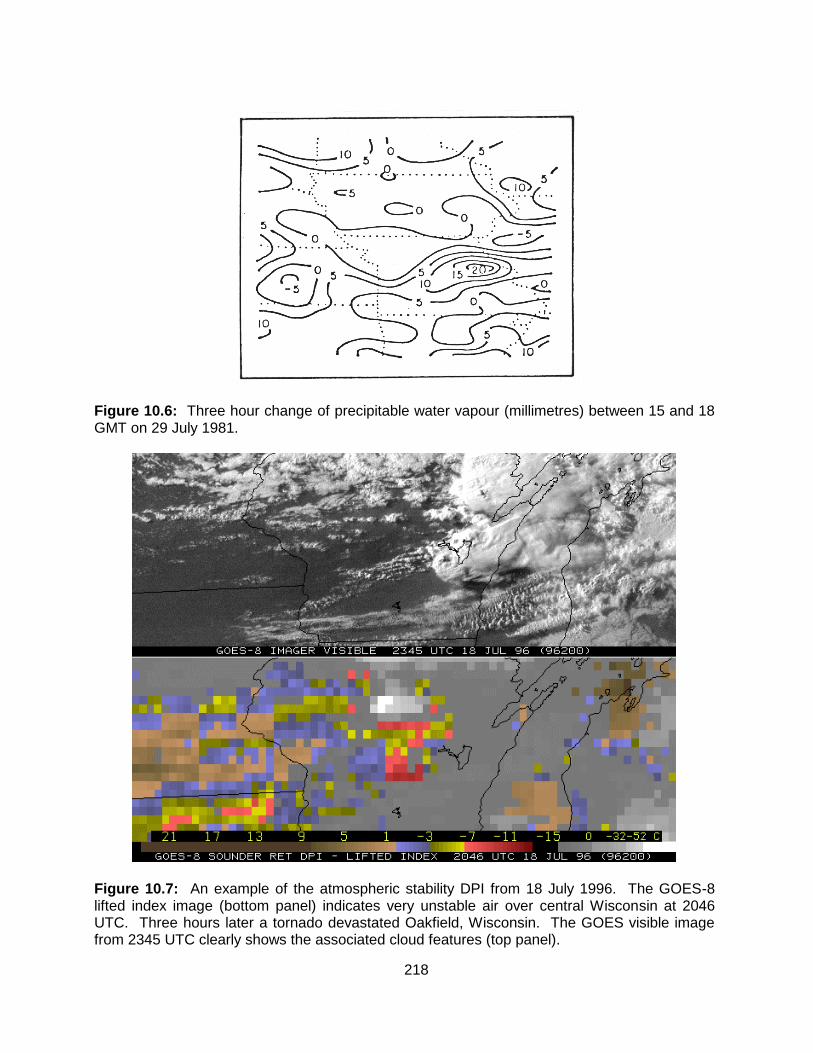
218
Figure 10.6: Three hour change of precipitable water vapour (millimetres) between 15 and 18 GMT on 29 July 1981.
Figure 10.7: An example of the atmospheric stability DPI from 18 July 1996. The GOES-8 lifted index image (bottom panel) indicates very unstable air over central Wisconsin at 2046 UTC. Three hours later a tornado devastated Oakfield, Wisconsin. The GOES visible image from 2345 UTC clearly shows the associated cloud features (top panel).

219
Figure 10.8: (top) GOES DPI of Lifted Index from 2046 to 0446 UTCat 2346 UTC on 25 June 1998 show extreme instability associated with a frontal passage across Minnesota and Wisconsin. (bottom) Radiosonde reports of lifted indices are overlaid on 2346 UTC DPI as are the wind reports.

220
Figure 10.9: (top) GOES DPI of Lifted Index from 1146 to 1746 UTC on 3 May 1999 show extreme instability associated with a frontal passage across Oklahoma and Texas. (bottom) Tornado in vicinity of Oklahoma City viewed at 0000 UTC.

221
Figure 10.10: Maximum temperatures forecast with and without GOES sounder data for 20 April 1997 in Madison, WI. Without sounder data a maximum temperature of 64 degrees F at 2100 UTC was forecast (9 hours after 1200 UTC, top panel) and with sounder data he forecast was adjusted to 59 degrees F at 1900 UTC (7 hours after 1200 UTC, middle panel); the surface observations report a maximum temperature of 58 degrees F at 2000 UTC (bottom panel).

222
CHAPTER 11
SATELLITE ORBITS
11.1 Orbital Mechanics
Newton's laws of motion provide the basis for the orbital mechanics. Newton's three laws are briefly (a) the law of inertia which states that a body at rest remains at rest and a body in motion remains in motion unless acted upon by a force, (b) force equals the rate of change of momentum for a body, and (c) the law of equal but opposite forces. For a two body system comprising of the earth and a much smaller object such as a satellite, the motion of the body in the central gravitational field can be written
dv / dt = -GM r / r
3
where v is the velocity of the body in its orbit, G is the universal gravitational constant (6.67 x 10
11 N m
2/ kg
2), M is the mass of the earth, and r is position vector from the centre of
mass of the system (assumed to be at the centre of the earth). The radial part of this equation has the more explicit form
m d2r/dt
2 - mrω
2 = -GMm/r
2
where ω is the angular velocity and m is the satellite mass. The second term on the left side of the equation is often referred to as the centrifugal force
The total energy of the body in its orbit is a constant and is given by the sum of the kinetic and potential energies
E = 1/2 m [(dr/dt)2 + r
2ω
2] - mMG/r .
The angular momentum is also conserved so that
L = mωr2 ,
which allows us to rewrite the energy
E = 1/2 m (dr/dt)2 + L
2/(2mr
2) - mMG/r .
The magnitude of the total energy reveals the type of orbit;
E > 0 implies an unbounded hyperbola,
E = 0 unbounded parabola,
E < 0 bounded ellipse,
E = -G2M
2m
3/(2L
2) bounded circle.

223
The last two terms of the total energy can be considered as an effective potential energy, which has a minimum for the radius of the circular orbit.
The circular orbit requires that the radius remain constant (so dr/dt equals zero) through the balance of the gravitational and centrifugal forces
GMm/r2 = mω
2r
or
r = L2/(m
2MG) .
This leads to the expression for the total energy of the satellite in a bounded circle.
It is also worth noting that the conservation of angular momentum is directly related to Kepler's law of equal areas swept out in equal time, since
dA/dt = r2ω/2 = L/(2m) = constant .
The derivative with respect to time can be rewritten as a derivative with respect to
angle through the conversion
d/dt = (L/mr2)d/dθ
so that
m d2r/dt
2 = (L/r
2)d/dθ[(L/mr
2)dr/dθ]
and using u = 1/r this becomes
[d2u/dθ
2 + u] = GMm
2/L
2 .
The solution has the form of the equation for a conic section
1/r = [GMm2/L
2] [1 + ε cosθ]
where the eccentricity ε is given by
ε2 = [1 + 2EL
2/(G
2M
2m
3)]
The point of closest approach, the perigee, occurs for θ = ; the apogee occurs for θ = 0.
11.2 The Geostationary Orbit
Let us continue our discussion of the circular orbit. Using the definition of angular
velocity ω = 2/ where is the period of the orbit, then
GMm/r2 = mω
2r
becomes

224
GM/r3 = 4
2/
2 .
For the geostationary orbit, the period of the satellite matches the rotational period of
the earth so that the satellite appears to stay in the same spot in the sky. This implies that = 24 hours = 8.64x10
4 seconds, and the associated radius of the orbit r = 4.24x10
7 meters or a
height of about 36,000 km. The geostationary orbit is possible at only one orbit radius.
For a polar circular orbit with = 100 minutes = 6x10⁴ seconds, we get r = 7.17x10
6
metres or a height of about 800 km. Polar orbits are not confined to a unique radius, however the type of global coverage usually suggests a range of orbit radii.
It is useful to note that
g = 9.8 m/s
2 = GM/R
2
where R is the earth radius (about 6.4x10
6 m) and GM ~ 3.986x10
14 m
3 / s
2.
11.3 Orbital Elements
A detailed knowledge of orbits allows the determination of what areas will be viewed by the satellite, how often, and when. Proper adjustment of the orbit can enhance repeated coverage of one area at the same time each day or repeated coverage of the same area every few minutes throughout the day. The coverage depends on six orbital elements.
To a first approximation a satellite close to the earth has an elliptical orbit. The orientation of the satellite orbit plane is described by (a) the inclination of the satellite orbit plane with respect to the earth equatorial plane denoted by I, and (b) the right ascension of the ascending node, Ω, measured eastwards relative to Aries (representing a fixed point in the heavens). The shape and size of the satellite orbit is given by (c) the semi-major axis of the ellipse denoted by a, and (d) the eccentricity of the ellipse, denoted by ε. The orientation of the orbit in the orbit plane is given by (e) the argument of the perigee or the angle between the ascending node and the perigee denoted by w. And finally (f) θ denotes the angular position of the satellite in its orbit. These are the six orbital elements that are necessary to calculate the trajectory of the satellite in its orbit; they are shown in Figures 11.1 and 11.2.
The geostationary orbit provides good temporal (half hourly) and spatial coverage over the equatorial regions (but its viewing angle to the polar regions is poor). On the other hand the polar orbit provides good coverage of the polar regions every 100 minutes (but its viewing over the equatorial regions is incomplete and less frequent). Thus studies over the tropics and the ITCZ (Inter Tropical Convergence Zone) rely mostly on geostationary satellite data, while the Arctic and Antarctic polar studies depend primarily on polar orbiting satellite data.
The elliptical orbit is an approximation; there are several small perturbing forces which are mentioned briefly here. (a) The earth is not spherical; it exhibits equatorial bulge which perturbs the orbital elements. This is an important correction; (b) Atmospheric drag significantly slows satellites below a height of 150 km, but is very small for orbit heights greater than 1500 km; (c) Solar wind and radiation slightly influence the orbit of satellites with low density; (d) The gravitational influence of the other bodies in the solar system, particularly the sun and the moon, are small but nonzero; (e) Relativistic effects are very small.

225
The primary influence of the non spherical earth gravitational field is to rotate the
orbital plane, to rotate the major axis within the orbital plane, and to change the period of the satellite.
11.4 Gravitational Attraction of Non-spherical Earth
The earth's gravitational field is not that of a point mass, rather it is the integrated sum over the bulging earth. The potential energy for a satellite of mass m a distance r from the centre of mass of the earth is written
PE = - Gm dM/s earth where the integration is over the mass increment dM of the earth which is a distance s from the satellite. This integration yields a function in the form
PE = -GMm/r [1 - Σ Jn (R/r)n Pn(cosθ)]
n=2,... where the Jn are coefficients of the n
th zonal harmonics of the earths gravitational potential
energy and the Pn (cosθ) are Legendre polynomials defined by
1 dn
Pn(x) = ___
____
[(x2-1)
n] .
n2n dx
n
The most significant departure from the spherically symmetric field comes from the n=2 term, which corrects for most of the effects of the equatorial bulge. Therefore
PE = -GMm/r [1 - J2 (R/r)2 (3cos
2θ - 1)/2 + ...]
where J2 = 1082.64x10
-6. At the poles P2 = 2 and at the equator P2 = -1. The coefficients for
the higher zonal harmonics are three orders of magnitude reduced from the coefficient of the second zonal harmonic.
Equatorial bulge primarily makes the angle of the ascending node vary with time.
11.5 Sun synchronous Polar Orbit
The equatorial bulge primarily makes the angle of the ascending node vary with time. The variation is given by
dΩ/dt = -3/2 J2 (GM) 1/2
R
2 a
-7/2 (1-ε
2)-2
cos i

226
Through suitable selection of the orbital inclination i, the rotation of the orbital plane can be made to match the rotation of the earth around the sun, yielding an orbit that is sun synchronous. The negative sign indicates a retrograde orbit, one with the satellite moving opposite to the direction of the earth’s rotation. The rotation rate for sun synchronous orbit is given by
Ω = 2/365.24 radians/year = 2 x 10 -7
rad/sec . which is approximately one degree per day. Such a rate is obtained by placing the satellite into an orbit with a suitable inclination; for a satellite at a height of 800 km (assuming the orbit is roughly circular so that a = r), we find i = 98.5 degrees which is a retrograde orbit inclined at 81.5 degrees. The inclination for sun synchronous orbits is only a weak function of satellite height; the high inclination allows the satellite to view almost the entire surface of the earth from pole to pole.

227
Figure 11.1: Orbital elements for an elliptical orbit showing the projection of the orbit on the surface of a spherical earth. C is the centre of the earth and R is the equatorial radius. i is the inclination of the orbit relative to the equatorial plane, Ω is the right ascension of the ascending node with respect to Aries, a is the semi-major axis of the ellipse, ε is the eccentricity, w is the argument of the perigee, and Θ is the angular position of the satellite in its orbit.
Figure 11.2: Elements of an elliptical orbit in the plane of the satellite orbit..

228
CHAPTER 12
RADIOMETER DESIGN CONSIDERATIONS
12.1 Components and Performance Characteristics
The optics, detectors, and electronics are the basic elements of a radiometer. Optics collect the radiation, separate or disperse the spectral components, and focus the radiation to a field stop. Detectors, located behind the field stop, respond to the photons with a voltage signal. That voltage signal is amplified by the electronics and converted into digital counts.
Performance of a radiometer is characterized by its responsivity, detectivity, and calibration. Responsivity is a measure of the output per input. Detectivity is expressed as the ratio of the responsivity per noise voltage. Calibration attempts to reference the output to known inputs.
12.2 Spectral Separation
Earth emitted radiation is detected in several spectral regions by radiometers where the spectral separation is accomplished by one of the following approaches. Prisms separate the incoming radiation as refraction changes with wavelength (bending angle depends on index of refraction that is a function of wavelength; longer wavelengths are deflected less). Band pass filters, using internal reflections within the filter, can separate the infrared spectrum into roughly 20 cm
-1 segments. Grating spectrometers (where path difference from slits produce positive
and negative wavelet interference on the detectors) and interferometers (where path differences or delays from two mirrors produces positive and negative wavelet interference) are
capable of spectral resolutions (λ / λ) of about 1 / 1000. All have been used for remote sensing of the earth. Figure 1 shows schematics for prism, grating and interferometer approaches for separating the spectrum.
12.3 Design Considerations
12.3.1 Diffraction
The mirror diameter defines the ability of the radiometer to resolve two point sources on the earth surface. The Rayleigh criterion indicates that the angle of separation , θ, between two points just resolved (maxima of the diffraction pattern one point lies on the minima of the diffraction pattern of the other point)
sin θ = λ / d where d is the diameter of the mirror and λ is the wavelength. The GOES satellite mirror diameter is 30 cm, so at infrared window wavelengths (10 microns) the resolution is about 1 km. This follows from 10
-5 m / 3 x 10
-1 m = 3.3 x 10
-5 = r / 36,000 km

229
or r = 1 km = resolution.
Diffraction is an important consideration when seeking clear FOVs in the vicinity of
clouds. Clouds can affect measured radiances even when they are not directly in the FOV of the sensor. When clouds are close enough to the FOV, diffraction causes some of the radiation received by the sensor to emanate from the clouds instead of from the clear area within the FOV. As clouds are typically colder than the clear earth-atmosphere, measured radiances are lower than expected from a clear FOV. Sensors in geostationary orbit are usually diffraction limited because the FOV is small for the mirror diameter in order to achieve maximum spatial resolution. Thus when sounding with the geostationary sounders, the clear FOV must be sufficiently far away from cloud contamination to assure correct profile retrieval or a correction must be applied for cloud diffraction into the FOV.
Figure 12.2.a shows the calculated diffraction effects for the new GOES imager for
infrared window radiation in a clear scene of brightness temperature 300 K surrounded by clouds of 220, 260, or 280 K. The size of the clear scene is varied and the change in brightness temperature is plotted. These results use a FOV radius of 2 km, a mirror diameter of 31 cm, and a wavelength of 11 microns. Diffraction effects are noticeable for clear scenes as large as 50 km radius; for a cold cloud at 220 K, the brightness temperature of a 10 radius clear hole is too cold by about 1.5 K. Figure 12.2.b shows the same plot for the GOES sounder infrared window with a 4 km radius FOV and the same optics; the diffraction effect is mitigated somewhat by the larger FOV of the sounder. Figure 12.2 indicates that to obtain clear sky brightness temperature within 1 K the clear area must be at least 15 km (10 km) in radius for the imager (sounder).
Diffraction is usually specified by encircled energy, the fraction of the total detected signal emanating from a circle of given size. For the GOES-8 imager infrared window this is given by 60% of the signal must come from a circle of one FOV diameter, 73% from 1.25 FOV diameter, and 79% from 1.5 FOV diameter. 12.3.2. The Impulse or Step Response Function
The detector collects the incident photons over a sampling time and accumulates a voltage response, which is filtered electronically. This is often characterized by the impulse (or step) response function, which details what the response of the sensor is to a delta (or step) function input signal. The response function is determined from the characteristics of the prealiasing filter which collects the voltage signal from the detector at the sampling times.
A perfect response of the detector continuously sampling a scene with a 100% contrast bar extending one FOV is indicated in Figure 12.3. As the detector crosses the contrast bar, the response ramps up linearly from 0 to 1 in the time it takes to move a distance of one FOV and then ramps down from 1 to 0 in a symmetric fashion. The actual response of the GOES-8 filter is also indicated in Figure 12.3. The shape and delay of the signal are noticeable. The filter delay causes an offset which can be corrected electronically. Sampling occurs every 183 microseconds or 1.75 times per FOV; the sampling interval is 4/7 of the time it takes to move one FOV.
Correcting for the time offset, the percentage of the total signal appearing in the samples preceeding and following the correlated sample peak can be estimated. For GOES-8

230
infrared window samples one finds that sample N-2 has 4.3% of the total signal, N-1 has 26.5%, N peaks with 44.8%, N+1 has 23.4%, and N+2 has 1.0%. This causes a smearing of cloud edges and other radiance gradients.
Figure 12.4 shows the step response function for GOES-8. The filter output takes about 400 (or about 2 samples) microseconds to respond full scale to the step function input at time t=0. 12.3.3 Detector Signal to Noise
The noise equivalent radiance for an infrared detector can be expressed as
NEDR() = [Ad f] 1/2
/ [Ao () Ω D* ] where
is the preamplifier degradation factor which includes the effects of both preamplifier noise and signal loading
Ad is the detector area in cm
2
f is the effective electronic bandwidth of the radiometer Ao is the mirror aperture area in cm
2
() is the transmission factor of the radiometer optics in the spectral interval Δ
Ω is the solid angle of the FOV in steradians
D* is the specific spectral detectivity of the detector in the spectral band in cm Hz
1/2 / Watt, and
is the spectral bandwidth of the radiometer at wavenumber in cm-1.
Figure 12.5 indicates the spectral regions where the InSb and HgCdTe detectors show skill in detecting infrared radiation. The values of NEDR for the GOES-8 imager are indicated below.
Band
Wavelength (micron)
Detector
NEDR (mW/m2/ster/cm-1)
NEDT
1
.52 - .75
Silicon
(3 of 1023 counts is noise)
2
3.83-4.03
InSb
0.0088
0.23 @ 300 K
3
6.5 - 7.0
HgCdTe
0.032
0.22 @ 230 K
4
10.2-11.2
HgCdTe
0.24
0.14 @ 300 K
5
11.5-12.5
HgCdTe
0.45
0.26 @ 300 K

231
12.3.4 Infrared Calibration
The radiometer detectors are assumed to have linear response to infrared radiation, where the target output voltage is given by
Vt = α Rt + Vo and Rt is the target input radiance, α is the radiometer responsivity, and Vo is the system offset voltage. The calibration consists of determining α and Vo. This is accomplished by exposing the radiometer to two different external radiation targets of known radiance. A blackbody of known temperature and space (assumed to emit no measurable radiance) are often used as the two references. If z refers to space, bb the blackbody, the calibration can be written as
Vz = α Rz + Vo
Vbb = α Rbb + Vo where
α = [Vbb - Vz]/[Rbb - Rz] and
Vo = [Rbb Vz - Rz Vbb]/[Rbb - Rz] Using Rz=0 this yields
Rt = Rbb [Vt - Vz] / [Vbb - Vz]. For HgCdTe detectors there sometimes is a non-linearity in the response to high
photon bombardment occurring in the infrared window. In this case the IR calibration equation is given by,
R = q C
2 + m C +b
where R = calibrated scene radiance (dropping the t for target),
C = digital counts (derived from the detector voltage with a linear analog to digital converter),
q = second order gain (non-linear term), m = first order gain (slope), and b = count offset.
The second order gain is estimated before launch in vacuum tests as a function of radiometer temperature. The first order gain is obtained from the blackbody and space looks in flight (as reported in Weinreb et al (1997) this occurs within every 20 minutes with GOES-8),
m = [Rbb - q (Cbb2 - Cz
2)] / [Cbb - Cz]
and the count offset is updated after every space look (about every 2 minutes for GOES-8) using,

232
b = -m Cz - q Cz
2
where Rbb is calculated from blackbody thermistor data telemetered down from the spacecraft, and
Cbb = digital counts during blackbody view, and Cz = digital counts during space view (before blackbody view).
The scan mirror of the radiometer telescope is usually not a perfect reflector, so there
is some emission from the mirror that must be accounted for in the calibration algorithm. If the scan mirror emissivity is isotropic (independent of viewing angle), then its contributions to the target, blackbody, and space looks is constant and does not affect the calibration algorithm. However if the scan mirror emissivity changes with viewing angle, then the radiance detected must be written
R` = [1 -ε(θ)] Rt + ε(θ) Rm
where Rm denotes the mirror emitted radiance, Rt is the target radiance, and ε(θ) is the scan mirror emissivity at angle θ. Then including the correction for the scan mirror emissivity variation, the first order gain is calculated after each blackbody view using,
m` = [Rbb` - q (Cbb2 - Cz
2)] / [Cbb - Cz]
where Rbb` = [1 -ε(θbb)] Rbb + [ε(θbb) - ε(θz)] Rm
and
θbb = scan mirror angle while viewing the blackbody (incidence angle of bb radiation is about 45 degrees),
θz = scan mirror angle while viewing space (at about 40 and 50 degrees), The offset is also adjusted through m`
b` = -m` Cz - q Cz2
The scan mirror emissivity corrected radiances are then calculated using,
R` = { q C2 + m` C +b` - [ε(θbb) - ε(θz)] Rm } / {1 -ε(θ)}
Figure 12.6 shows the emissivity changes with angle and wavelength for the GOES-8 scan mirror. The radiance corrections, ΔR = R` - R, for GOES-8 infrared window radiances are about 2 mW/m
2/ster/cm
-1 which convert to 1.2 C for a scene of 300 K.
The GOES-VAS satellites, which spin at 100 rpm, experience small diurnal
temperature excursions. However, the GOES-8/9 satellites are three-axes stabilized so temperatures within the sensors vary by tens of degrees K over a 24 hour period. Therefore, the coefficients in the calibration equation must be updated frequently. To accomplish this, both the imager and the sounder view space routinely. The sounder views its blackbody every twenty minutes, while the imager normally views its blackbody every ten minutes unless doing

233
so interrupts an image in process. At the most, the imager operates 30 minutes between blackbody views, e.g., when it makes a full-disk image. Drift in detector response (often referred to as 1/f noise (Bak et al. 1987)) dictates that the space and blackbody calibration looks occur frequently enough to keep changes in calibration within the specified noise levels. The ground system processing interpolates between calibration events, so that different calibration coefficients are determined for each data sample to account for the linear portion of the detector drift. 12.3.5 Bit Depth
The range of radiances expected for earth and atmosphere in a given spectral band must be converted to digital counts of fixed bit depth. This introduces truncation error. For n bit data, the radiance range, must be covered in 2
n even increments. Consider the GOES-8
imager truncation errors indicated in the following table.
Band
Bit Depth
Rmax
ΔR
Tmax
ΔT(230)
ΔT(300)
(micron)
(mW/m2/ster/cm-1)
(degrees Kelvin)
1
.65
10
(more detail in images)
2
3.9
10
3.31
0.003
335
2.14
0.09
3
6.7
10
48.3
0.047
320
0.33
0.06
4
10.7
10
147.7
0.144
320
0.20
0.09
5
12.0
10
166.5
0.163
320
0.19
0.09
For earth scenes of 300 K, the truncation errors are small, less than a tenth of a degree Kelvin. However for cloud scenes of 230 K, the errors become greater than 2 K in the 3.9 micron band; this causes clouds to appear very noisy in this spectral band.
It is important that the truncation error is less than the error introduced by detector noise; this is true for GOES-8 since the NEDT at 300 K is about 0.2 C.
12.4 Establishing Sensor to Sensor Intercalibration The more than 30 years of observations from instruments (AVHRR, HIRS, MSU) aboard NOAA series of satellites have been widely used in numerical weather prediction and climate studies. However, there are significant discrepancies in the radiance measurements between different satellites. To ensure the consistency and reduce the uncertainties for the climate studies, inter-satellite radiance comparisons have been undertaken at Simultaneous-Nadir-Overpass (SNO) locations for the NOAA series of satellites (Cao et al. 2004). Figure 12.7.a illustrates the concept for achieving an integrated Global Observing System using intersatellite calibration of low earth orbiting (LEO) and geostationary (GEO) satellite instruments at the moment of SNO. Chen et al. (2012) have performed inter-satellite radiance comparisons at SNO locations for HIRS longwave CO2 channels on-board the NOAA and Metop series of

234
satellites. The high spectral resolution measurements from the Infrared Atmospheric Sounding Interferometer (IASI) on the Metop-A satellite were used to simulate the HIRS observations; the IASI measurements are convolved with the pre-launch HIRS Spectral Response Functions (SRF) to create simulated HIRS radiances. These are compared to the collocated measured HIRS radiances; the pre-launch SRF is then adjusted to minimize the difference between HIRS simulated and measured radainces. In this way the Metop-A HIRS is established as a reference HIRS for the earlier HIRS sensors that can be recalibrated via SNOs; Figure 12.7.b illustrates this process. The inter-satellite mean radiance biases are minimized towards zero with residual maximum uncertainty less than 1% after the impacts of SRF differences and uncertainties are taken out. Compared with pre-launch SRF measurements, the optimized shifts of the SRF can be as large as 2.5 cm-1; this can cause radiance adjustments of up to 3 mW/m
2/ster/cm
-1 or
brightness temperature changes of up to 2 K (see Figure 12.7.c). Chen et al. (2013) found that the inter-satellite radiance biases as large as 5% were reduced to less than 1% for the HIRS CO2 channels after the spectral shifts suggested by this process (Figure 12.7.d). 12.5 Sounding with an Interferometer
The goal of sounding with an interferometer is to obtain high vertical resolution atmospheric emission information from a high-frequency portion of an interferogram. An interferogram (the Fourier transform of the spectrum) is the basic measurement of Michelson-
type interferometer. Whereas a spectral radiance measurement at a particular wavenumber examines emission due to a particular line (providing the spectral resolution is very high), the interferogram signal measures the interference of two radiation streams (caused by a phase delay δ) for all absorption lines in the spectrum. In the recombined radiance for certain δ, the
interference increases contributions from some layers of the atmosphere while reducing contributions from other layers. The net result is vertical temperature profile weighting functions in interferogram space (coordinates) which are more independent of each other and narrower in certain atmospheric regions than can be achieved in spectral space with practical spectral resolutions and current instrument accuracies. State-of-the-art interferometers of relatively simple design collect energy selectively over a wide range of wavelengths applicable to the temperature sounding problem.
In a noise-free environment, if a complete spectrum of radiance with infinite spectral resolution were obtainable, it would contain precisely the same information as a complete interferogram (the one being the Fourier Transform of the other). However, the information content of a limited portion of an interferogram is much different from that of a limited spectrum of finite spectral resolution, and these differences are exaggerated when considering realistic measurement noise. It can be shown that the information contained in a portion of an interferogram is equivalent to that in the difference between a high- and low-resolution radiance spectrum, their resolutions being a function of the beginning and ending delays of the interferogram. The difference between spectra of atmospheric radiance at two different spectral resolutions depends strongly on the lapse rate of temperature. Thus, the observations contained in a partial interferogram are more sensitive to atmospheric structure than are the observations contained in a single radiance spectrum, given the same measurement noise level. It is the unique information and noise characteristics of observations by a partial interferogram

235
which we propose to exploit to dramatically improve the vertical resolution and profiling accuracy with a practical “state-of-the-art” instrumental approach to the sounding problem.
Neglecting instrument geometrical factors, Figure 12.1 (bottom panel) shows that the intensity of radiation I(δ) on the detector of a Michelson-type (two-beam) interferometer is
proportional to the square of the sum of the amplitudes of the two beams, traversing different optical paths before recombining at the detector. Taking into account their phase difference for
monochromatic radiation ( 0)
2 2 1( ) 4 cos ( / ) ( )[1 cos(2 )]
2I a I v v , (1)
where a is the amplitude of the incident radiation, δ the phase difference (delay), λ the
wavelength, ν=1/λ the wave number, and I(ν) the intensity of radiation for zero phase difference
(for an ideal instrument this is equal to the radiance from the source). In practice, viewing the earth’s non-monochromatic spectral radiance distribution, the spectrally integrated intensity (radiance) observed by the interferometer would be given by
0
1( ) ( )[1 cos(2 )]
2F I v v dv
. (2)
If we limit the input the instrument to a spectral region 1 2v v by an interference filter with a
transmittance of ( )f v within the bandpass region, the (2) becomes
2
1
1( ) ( ) ( )[1 cos(2 )]
2F I v f v v dv
. (3)
During delay scanning the delay-independent part of the integrand can be eliminated by a simple bandpass filter. The resulting signal (multiplied by 2 for convenience) is given by
2
1
( ) 2 ( ) (0) ( ) ( )cos(2 )S F F I v f v v dv
, (4)
where 2
1
(0) ( ) ( )
v
v
F I v f v dv . (5)
To simplify, we assume a perfect filter, ( ) 1.0f v . Thus, the interferometer signal at delay δ is a
cosine-weighted integrated intensity over the spectral region 1 2v v .
Figure 12.8.a shows an interferogram computed for a standard atmospheric condition assuming a square wave interference filter limiting the input energy to the 15 μm CO2 band, 600-750 cm
-1. (for this calculation, a spectral resolution of 0.1 cm
-1 and a delay resolution of 0.002
cm were used. It is noted that much more time-consuming calculation with a spectral resolution of 0.02 cm
-1 were also made to verify the adequacy of utilizing 0.1 cm
-1 spectra for these and
subsequent interferogram simulations.) As can be seen, there are amplitude peaks near 0.6, 1.2 and 1.8 cm delays resulting from the nearly uniform 1.6 cm
-1 (0.6 cm wavelength) spacing of

236
the CO2 lines. These resonances occur at delays which are multiples of the wavelength spacing of the lines (inverse of the line spacing in wavenumbers), and as a result, purely constructive interference results. At intermediate delays (e.g., 0.3, 0.9, 1.5 cm, etc.) there is a tendency for
compensating contributions from the various lines in the 1 2v v frequency interval so that the
amplitude of the interferogram is near zero in these delay regions.
The advantage to interpreting interferogram radiance signals rather than spectral radiance measurements for determining atmospheric structure involves two elements – improved weighting function characteristics and equivalent signal-to-noise ratios in the observations. 12.5.1 Interferograms
The interferogram S(δ) in mW/m2/ster as a function of the phase difference (delay) δ (cm)
within an interferometer and the spectrum (spectral radiance) I() in mW/m2/ster as a function of
wave number (cm-1) are Fourier transforms of each other. In case of symmetric interferograms
only the cosine transformation is needed. Hence,
0
( ) ( ) ( )cos(2 )S I v g v v dv
and
0
( ) ( ) ( )cos(2 )g v I v S v d
(6)
Where g(ν) is the spectral instrument response function. In compliance with (1) the whole
interferogram and the entire spectrum contain precisely identical information. Actually, however,
the delay δ is restricted to a limited interval with max and the spectral bandpass to a spectral
region (ν1, ν2). The spectral resolution element f(ν) of a spectrum obtained from an interferogram
with delays between 1 0 and 2 max is in case of a rectangle spectral response function
g(ν)=1 the function of sin x/x, the sinc function
f maxmax max max
max
sin(2 )( ) 2 2 sin (2 )
2
vv v
v
c (7)
Partially scanned, i.e., partial interferograms are defined by delays starting from 1 min 0 . In
this case, f(ν) is given by
f max max min min( ) 2 sin (2 ) 2 sin (2 )v v v c c (8)
The spectral resolution in case of a non-apodized spectrum resulting from an interferogram with
delays between 1 0 and 2 max is given by
max
1
2v
(9)

237
There is no accurate physical meaning of spectral resolution for partial interferograms. According to (8) a partial interferogram contains only information equivalent to the difference between a spectrum of high spectral resolution (Δν ~ 1/2δmax) and a spectrum of minor spectral
resolution (Δν ~ 1/2δmin). Hence, the information contents of partial interferograms and of the
corresponding spectra are totally different. According to (6) interferograms with a delay δ contain information of each absorption line of a spectrum whereas the spectrum contains only information of a limited spectral interval defined by the spectral resolution Δν. It is this difference
between the information content of spectra and interferograms that gave rise to the aforementioned considerations. 12.5.2 Theoretical Calculation of Partial Interferograms
The spectral radiance measured by a satellite spectrometer viewing into the direction Θ to the nadir is
R
ln( , )
( ) [ ] ( , ) [ ( )] lnln
sp
vv s v s v
pv B T p B T p d p
p
(10)
with Bν(T) as the blackbody (Planck) radiation at temperature T and wave number ν, temperature
profile T(p), surface temperature Ts and spectral atmospheric transmittance v between p and
the pressure level indicated. Without any restriction the Θ-dependence is omitted hereafter.
The corresponding partial interferogram for the wave number domain 1 2[ , ]v v is
2 2
1 1
ln( )
( ) [ ] ( )cos(2 ) [ ( )] cos(2 ) lnln
sp
v s s
pS B T p d B T p d d p
p
(11)
which would have been measured by an interferometer as a function of delay δ. Defining the
transmittance
2
1
* ( ) ( )cos(2 )p p d
(12)
and the weighting function
2
1
* ( ) ( )(2 )
ln ln
p pocs dv
p p
(13)
in the interferogram space at a fixed delay δ. With (12) and (13) we obtain for (12)
** ( )
( ) ( ) ( ) [ ( )] lnln
sLnp
s s
pS p B T B T p d p
p
(14)
where B is the weighted mean Planck radiance of the spectral interval . Equation (14) is formally identical with the conventional remote sounding Equation (10). Hence, the analysis of

238
retrieval accuracy and cloud elimination in case of partial interferograms can be made by exactly the same conventional mathematical procedures. Restricting the spectral range to the CO2 band system from 600 cm
-1 to 750 cm
-1, it can be shown that the delay δ can be limited to the interval
0 2 cm. Within this interval the regions 0 to 0.24 cm, 0.59 to 0.70 cm, 1.26 to 1.4 cm and
1.8 to 2.0 cm are of interest since – due to the nearly uniform line spacing of ν2 – CO2 absorption
lines of 1.5 cm-1 equivalent to a delay of δ ~ 0.6 cm – it is only there that sufficient intensity is
available.
The intensity in interferogram space decreases in the above-mentioned regions with increasing δ. The energetically most suitable region is therefore from 0 to 0.24 cm, and the
energetically less suitable one is from 1.8 to 2.0 cm. The 0 to 0.24 cm delay corresponds to a near-complete interferogram and is equivalent to a spectrum with spectral resolution of about 2 cm
-1. One of the first interferometers in the Earth’s orbit in the 1969, Infrared Interferometer
Spectrometer (IRIS) worked in this regime (Hanel et al. 1971). Subsequently, simulations have shown that the 0.59 to 0.70 cm interval gives the highest accuracy in temperature retrievals. 12.5.3. The weighting function
Considering the radiative transfer equation in the form
0
0
( )( ) ( ) ln
ln
p
s s
d vI v B v B p
d p
(15)
where B is the Planck radiance, τ the transmittance, p pressure and the subscript s refers to
surface conditions, it follows that
0 **
0
( ) lnln
p
s s
dS B B d p
d p
(16)
where B is the mean Planck radiance for the spectral interval,
2
1
* ( )cos(2 )
v
v
v v dv
and 2
1
*
cos(2 )ln ln
v
v
d dv dv
d p d p
(17)
The weighting function * / lnd d p in interferogram space is for a fixed delay δ. It is a cosine-
weighted combination of the monochromatic spectral weighting functions over the 1 2v v interval.
Figure 12.8.b shows interferogram weighting functions of the 15 μm band (600-750 cm-1)
for four different delays. These examples represent a selection from the region of resonance near 1.2 cm. The weighting functions have been averaged over a 0.001 cm interval to simulate the maximum delay smearing caused by the non-flatness of the optical components to be encountered in a practical instrument. In terms of vertical resolution, the width of the main lobe is slightly greater than one-half a scale height (~5 km) or, in other terms, slightly greater than

239
half that of monochromatic spectral radiance weighting functions. Unlike the latter, however, the interference radiance weighting functions have side lobes, which must be accounted for in the radiance-to-temperature inversion process, making the true vertical resolving power of a single observation less than that implied by the main lobe alone. The important difference between weighting functions in spectral and interference coordinates is not, however, the resolving power of a single observation, but rather the vertical independence of each observation within a set (i.e., spectrometer measurements at several frequencies or interferograms at several delays). Figure 12.8.c depicts a set of weighting functions for spectral radiances of 0.5 cm
-1 resolution.
Comparing this figure with Figure 12.8.b, one notices a higher frequency structure in the case of the interferometric weighting functions indicating a greater degree of vertical independence. The variations in some atmospheric layers can be detected more readily with the set of interference radiance observations. For example, suppose that the only difference between two atmospheric states is the temperature near 300 mb. In the interference case (Figure 12.8.b) only two measurements will vary significantly between atmospheric states (i.e., the δ = 1.17 and δ = 1.76
cm), whereas in the spectral case (Figure 12.8.c) all four observations will be influenced significantly by the 300 hPa temperature variation. This feature alone would lead to improved vertical resolution in retrieved thermal profiles if the signal-to-noise ratio of interference measurements were comparable to the spectral observations. References Aumann, H. H., M. T. Moustafa, C. Gautier, M. D. Goldberg, E. Kalnay, L. M. McMillin, H.
Revercomb, P. W. Rosenkranz, W. L. Smith, D. H. Staelin, L. Strow, and J. Susskind, 2003: AIRS/AMSU/HSB on the Aqua mission: Design, Science Objectives, Data Products, and
Processing Systems. IEEE Trans. Geosci. Remote Sens., 41, 253-264. Cao, C., M. Weinreb, and H. Xu, 2004: Predicting simultaneous nadir overpasses among polar-
orbiting meteorological satellites for the intersatellite calibration of radiometers. J. Atmos. Oceanic Tech., 21, 537-542.
Cao, C., M. Goldberg, L. Wang, 2009: Spectral Bias Estimation of Historical HIRS Using IASI Observations for Improved Fundamental Climate Data Records. Journal of Atmospheric and Oceanic Technology, 26:7, 1378-1387
Chen, R., C. Cao, and W. P. Menzel, 2013: Inter-satellite Calibration of NOAA HIRS CO2 Channels to Ensure the Long-term Time Series Consistency for Climate Studies. Submitted to J. Geophys. Res.–Atmos.
Hanel, R. A., B. Schlachman, F. D. Clark, C. H. Prokesh, J. B. Taylor, W. M. Wilson, and L.
Chaney, 1970: The NIMBUS-3 Michelson Interferometer. Appl. Optics, 9, 1767-1773. Kaplan, L. D., M. T. Chahine, J. Susskind, J. E. Searl, 1977: Spectral band passes for high
precision satellite sounder. Appl. Optics, 16, 322-325. Smith, W. L., H. B. Howell, and H. M. Woolf, 1979: The Use of Interferometric Radiance
Measurements for Sounding the Atmosphere. Jour Atmospheric Sciences, 36, 566+ Weinreb, M., M. Jamieson, N. Fulton, Y. Chen, J. X. Johnson, J. Bremer, C. Smith, and J.
Baucom, 1997: Operational calibration of Geostationary Operational Environmental Satellite-8 and-9 imagers and sounders. Applied Optics, Vol. 36, Issue 27, pp. 6895-6904 http://dx.doi.org/10.1364/AO.36.006895

240
Spectral Separation with a Prism: longer wavelengths deflected less
Spectral Separation with a Grating: path difference from slits
produces positive and negative wavelet interference on screen
Spectral Separation with an Interferometer - path difference
(or delay) from two mirrors produces positive and negative wavelet interference
Figure 12.1: Prism, grating, and interferometer approaches for spectral separation

241
Figure 12.2.a: Calculated diffraction effects for GOES imager infrared window radiation with a 2 km radius FOV in a clear scene of brightness temperature 300 K surrounded by clouds of 220, 260, or 280 K.
Figure 12.2.b: Same plot for GOES sounder infrared window with a 4 km radius FOV and the same optics.

242
Detector
scanning across
feature of
finite dimension
Figure 12.3: Perfect and actual response of the GOES-8 detector continuously sampling a scene with a 100% contrast bar extending one FOV.
Figure 12.4: The step response function for GOES-8.

243
Figure 12.5: Detectivity of InSb and HgCdTe detectors as a function of spectral region.
Figure 12.6: Emissivity changes with angle and wavelength for GOES-8 scan mirror.

244
Figure 12.7.a: Illustration of Intersatellite Calibration of LEO and GEO using the Simultaneous Nadir Overpass (SNO) Method.
Figure 12.7.b: Inter-satellite calibration process for the HIRS on the NOAA satellite series, using Metop-A HIRS as a reference sensor.

245
Figure 12.7.c: Using IASI to adjust HIRS Spectral Response Functions (SRFs) illustrated function HIRS band 5 (at 14.0 µm or 715 cm
-1). A shift of 2.5 cm
-1 can cause a discrepancy
between observed and calculated radiance of about 3 mW/m2/ster/cm
-1 (equivalent to a
brightness temperature change of about 2 K).
Figure 12.7.d: (left column) Inter-satellite SRF shifts suggested by the SNOs. The blue bar represents data from north pole and red bar represents data from south pole. (right column) The accumulated changes of center wave number (right column) for HIRS on board NOAA-9 to NOAA-19 to match the Metop-A HIRS SRF radiances.

246
Figure 12.8.a: Interferogram for the 15 micron CO2 band (600 – 750 cm-1) computed for the
U.S Standard Atmosphere
Figure 12.8.b: Interferometric radiance temperature profile weighting function for several delays.

247
Figure 12.8.c: Spectral radiance temperature profile weighting functions for several frequencies.

248
CHAPTER 13
ESTABLISHING CLIMATE DATA RECORDS
FROM MULTISPECTRAL MODIS MEASUREMENTS
13.1 The MODIS Spectral Bands
The Moderate Resolution Imaging Spectroradiometer (MODIS) is an Earth Observing System (EOS) facility instrument that is currently flying aboard the Terra and Aqua spacecraft. It is especially well suited to global monitoring of atmospheric properties from space, and is based on heritage sensors such as the Advanced Very High Resolution Radiometer (AVHRR), Landsat Thematic Mapper (TM), High-resolution Infrared Radiation Sounder (HIRS), and the Nimbus-7 Coastal Zone Color Scanner (CZCS). The MODIS is a scanning spectro-radiometer
with 36 spectral bands between 0.645 and 14.235 m (King et al. 1992). Table 13.1 lists the MODIS spectral channels and their primary application. Bands 1 - 2 are sensed with a spatial resolution of 250 m, bands 3 - 7 at 500 m, and the remaining bands 8 – 36 at 1000 m. The signal to noise ratio in the reflective bands ranges from 50 to 1000; the noise equivalent temperature difference in the emissive bands ranges from 0.1 to 0.5 K (larger at longer wavelengths). Figure 13.1 shows the spectral bands superimposed on the earth reflection and
emission spectra.
13.2 Climate Questions 13.2.1 Energy Balance
The flow of radiation from the Sun to the Earth, its absorption, reflection, and emission, determines the energy balance of the Earth, and hence the nature of the life of its inhabitants. The information from products describing optical and physical properties of clouds and aerosols is combined with broadband radiation measurements to provide estimates of solar and infrared radiative fluxes, which, in turn, determine the heating and cooling of the Earth and the atmosphere. The necessary radiation estimates are shortwave and longwave fluxes at the surface and top of the atmosphere, both downwelling and upwelling, so that the net flow can be determined. Fluxes must be distinguished between cloudy and clear-sky regions as the flow of energy to and from the Earth is modulated by clouds and aerosols. Measuring and understanding these elements are keys to predicting climate change and to testing global climate models. The technology for accurately measuring radiative fluxes, cloud properties, and aerosol properties from space has advanced to the point that these observations can be used to greatly advance our ability to address critical global change issues. For example, if the global climate changes, do clouds generate a positive or negative feedback? Do aerosols offset some of the expected warming due to the increase in greenhouse gases? Figure 13.2 indicates the annual mean global energy balance for the earth-atmosphere system. Tracking the global energy balance trends is a vital part of climate change research.
Clouds: A key step in measuring cloud properties from space is to determine where clouds exist, how they are distributed through the atmosphere, and what their dimensions are. Once clouds are identified and mapped, cloud properties, such as effective particle size,

249
thermodynamic phase (water, ice), cloud top properties, and optical thickness (which all help determine how much radiation passes through them), may be measured. These cloud properties help to determine how much solar radiation reaches the Earth and how much escapes back to space. They also supply information on factors that influence cloud formation and forces driving circulation and global climate. Cloud detection and delineation produces masks indicating where clouds exist and information on layering and overlap to give a geometric picture of global cloud coverage. Cloud property retrieval quantifies the physics of the cloud through parameters such as optical thickness, temperature, liquid water content, ice water content, particle radius, cloud top altitude, and phase, which all relate to the radiative transmission, reflection, and emission of the cloud. A thorough description of global cloudiness and its associated properties is essential because (a) clouds play a critical role in the radiative balance of the Earth and must be accurately described in order to assess climate and potential climate change accurately and (b) the presence or absence of clouds must be accurately determined in order to retrieve properly many atmospheric and surface parameters where often even thin cirrus represents contamination.
Aerosols: The measurement of aerosols, suspended particles in the atmosphere (e.g., dust, sulfate, smoke, etc.), is an important element in describing energy transmission through the atmosphere. Aerosols are a significant source of uncertainty in climate modeling because they affect cloud microphysics by acting as condensation nuclei, thereby affecting cloud radiative properties, the hydrological cycle and atmospheric dynamics. They also interact directly with solar radiation, thus affecting the radiative balance. The location of anthropogenic aerosols is also an important consideration in their impact on climate.
Radiant Energy Flux is an estimate of the radiative flux downward and upward at the top-of-atmosphere, at the Earth’s surface, and at selected intermediate altitudes, as well as the net flux, which is used to determine the radiation budget. This budget determines the overall heating and cooling of the atmosphere and Earth’s surface and subsequent changes in climate. 13.2.2 The Water Cycle
The hydrological cycle is one of three key Earth system processes that are components of global climate; along with the carbon and energy cycles. Monitoring precipitation and atmospheric humidity is critical to obtaining hydrological-cycle parameters needed for developing global climate models and detecting climate change. The processes that generate rainfall are central to the dynamical, biological, and chemical processes in the atmosphere, in the oceans, and on the land surfaces. Space-based measurements give a more accurate global documentation of tropical rainfall.
The principal research objective is to explore the connection between weather processes and climate change and the fast dynamical/physical processes that govern climate responses and feedbacks. Particularly significant is the transformation of water among its three physical states - vapor, liquid, and solid - in the atmosphere and at the surface of the Earth. The condensation of water in cloud and snow control both the albedo and radiation balance of the planet, and the constant renewal of fresh water resources. The development of weather systems and the associated cloud life cycles play a key role in the water and atmospheric energy. A central science objective is exploring the responses of hydrologic regimes to changes in climate (precipitation, evaporation, and surface run-off) and the influence of surface hydrology (soil moisture, snow accumulation and soil freezing) on climate. Figure 13.3 gives a

250
schematic of the motions associated with individual water molecules between the oceans, water vapor in the atmosphere, water and ice on the land, and underground water.
Precipitation: The majority of global precipitation occurs in the tropics, between latitudes of 30°N and 30°S. Tropical rain is one of the key parameters that affects the global heat balance and the global water cycle. To understand and predict large variations in weather and climate, it is critical to understand the coupling between the atmosphere and the surface below, which is approximately 29% land and 71% ocean. Atmospheric circulation transports both energy and water, moving heat from the tropics to the polar regions. Water that has evaporated from the oceans and the land surface falls as rain or snow, often in places far removed from its point of origin. There is evidence that tropical rainfall variability, apparently coupled with changes in the underlying surface (particularly sea surface temperature), is associated with significant alterations in wind patterns and rainfall. Fluctuations in rainfall amount impact climate on both short and long time scales. Unlike the small-scale general features that appear on daily weather maps, the long-term, time-averaged circulation and precipitation fields show large-scale features associated with the annual evolution of the monsoons, trade wind systems, and oceanic convergence zones. Large-scale features are also evident on a monthly and seasonal scale. Inter-annual variability is dominated by tropical Pacific ocean-atmosphere interactions. These interactions are associated with the El Niño-Southern Oscillation (ENSO) cycle, whose major swings, which occur at irregular intervals of two to seven years, are associated with pronounced year-to-year precipitation variations over large areas of the tropics. The large-scale spatial coherence and systematic evolution of both intra-seasonal and inter-annual tropical precipitation anomalies is of great significance to climate prediction. They are also important in the development of optimal sampling strategies for estimating accumulated precipitation over periods of a few weeks to a few months. The characterization of rainfall in tropical regimes is fundamental to improving techniques of radar-rainfall measurements as well. Not only are there regional and seasonal differences, but significant differences also occur within tropical rain systems. These differences can be broadly classified as 1) morphological, referring to sizes, lifetimes, and spatial structures of rain-producing systems; and 2) microphysical, referring to raindrop formation processes, and the raindrop size distribution. Rainfall rates display a highly variable structure in both time and space, meaning radar surveillance systems must take frequent measurements to accurately assess rainfall totals. Three dimensional volume scans (like the WSR-88D radar scans on the nightly weather reports) every five minutes are desirable, although scans at 15-minute intervals provide useful data. The hydrological and severe weather monitoring requirements of most operational radar systems satisfy these criteria, providing invaluable ground-based validation data with nominal additional expenditure.
Humidity: Atmospheric circulation redistributes moisture and heat. Water vapor evaporates from the ocean and land surfaces, and is transported to other parts of the atmosphere where condensation occurs, clouds form, and precipitation ensues. There is a net outflow of atmospheric moisture from the tropics, where sea-surface temperatures are high and the warm atmosphere can hold large amounts of water vapor, to higher latitudes, where condensation and precipitation remove the moisture. Current numerical weather prediction models give inconsistent results about the future distribution of precipitation. Humidity is the amount of water vapor in the atmosphere. Water vapor concentration depends on temperature, which determines the total amount of water that the atmosphere can hold without saturation. Hence, water vapor amounts decrease from Equator to Pole and with increasing altitude. Generally, water amounts are less over the continents than over the oceans, and the upper atmosphere is drier than the near-surface atmosphere. Superimposed on this general behavior

251
are smaller variations of water vapor amounts that determine the formation and properties of clouds and rainfall. 13.2.3 The Carbon Cycle
In addition to the natural fluxes of carbon through the Earth system, anthropogenic (human) activities, particularly fossil fuel burning and deforestation, are also releasing carbon dioxide into the atmosphere. When we mine coal and extract oil from the Earth’s crust, and then burn these fossil fuels for transportation, heating, cooking, electricity, and manufacturing, we are effectively moving carbon more rapidly into the atmosphere than is being removed naturally through the sedimentation of carbon, ultimately causing atmospheric carbon dioxide concentrations to increase. Also, by clearing forests to support agriculture, we are transferring carbon from living biomass into the atmosphere (dry wood is about 50 percent carbon). The result is that humans are adding ever-increasing amounts of extra carbon dioxide into the atmosphere. Because of this, atmospheric carbon dioxide concentrations are higher today than they have been over the last half-million years or longer.
Not all of the carbon dioxide that has been emitted by human activities remains in the atmosphere. The oceans have absorbed some of it because as the carbon dioxide in the atmosphere increases it drives diffusion of carbon dioxide into the oceans. However, when we try to account for sources and sinks for carbon dioxide in the atmosphere we uncover some mysteries. For example, notice in Figure 13.4 (schematic of the carbon cycle) that fossil fuel burning releases roughly 5.5 gigatons of carbon (GtC [giga=1 billion]) per year into the atmosphere and that land-use changes such as deforestation contribute roughly 1.6 GtC per year. Measurements of atmospheric carbon dioxide levels (going on since 1957) suggest that of the approximate total amount of 7.1 GtC released per year by human activities, approximately 3.2 GtC remain in the atmosphere, resulting in an increase in atmospheric carbon dioxide. In addition, approximately 2 GtC diffuses into the world’s oceans, thus leaving 1.9 GtC unaccounted for.
What happens to the leftover 1.9 GtC? Scientists don’t know for sure, but evidence points to the land surface. However, at this time, scientists do not agree on which processes dominate, or in what regions of the Earth this missing carbon flux occurs. Several scenarios could cause the land to take up more carbon dioxide than is released each year. For example, re-growth of forests since the massive deforestation in the Northern Hemisphere over the last century could account for some of the missing carbon while changing climate could also contribute to greater uptake than release. The missing carbon problem illustrates the complexity of biogeochemical cycles, especially those in which living organisms play an important role. It is critically important that we understand the processes that control these sources and sinks so that we can predict their behavior in the future. Will these sinks continue to help soak up the carbon dioxide that we are producing? Or will they stop or even reverse and aggravate the atmospheric increases? With the use of satellites and field studies, scientists will help to obtain crucial information on the carbon cycle.
13.3 MODIS Product Descriptions
MODIS products are indicated in Table 13.2. The MODIS spectral bands have been chosen to be sensitive to various reflection, absorption, and scattering spectral signatures. Figures 13.5a-d show some of these features. Figure 13.6 shows the processing schema used

252
for deriving atmospheric products from level 0 (raw instrument data) to level 1 (calibrated earth located radiances) to level 2 (5x5 field of view derived atmospheric products) to level 3 (time composited global product fields in even interval lat-lon grid boxes). The following sections outline some of the considerations necessary when deriving some of these products. 13.3.1 Cloud Mask
Cloud measurements are important because clouds often obscure the Earth’s surface, complicating measurements of land surface conditions such as vegetative cover or sea surface temperature. At the time of any individual satellite overpass, the Earth scene below MODIS may be covered with clouds. However, the exact same areas aren’t likely to be cloudy every day, and scientists can combine, or composite, data over many days to produce weekly and monthly cloud-cleared products that can be used as input to global change models. MODIS’s cloud-detection capability is so sensitive that it can even detect clouds that are indistinguishable to the human eye.
The MODIS cloud mask (MOD35) is a global product that provides a probability that a
view of the Earth is obstructed by cloud and whether cloud shadow is detected. It also provides information on the processing path taken by the algorithm (land/sea, day/night, etc.), along with individual spectral test results used in the determination of the final cloud mask product. Cloud physical properties are obtained using a set of algorithms operating on multispectral imagery data from multiple sources. Cloud property parameters include particle size and phase, optical thickness, cloud top height, emissivity and temperature, and cloud fraction in a region, all of which support specific MODIS science tasks that complement the radiation studies and products from other instruments. By using many bands in the visible, near-infrared, and infrared portions of the spectrum at 1 km resolution, improved discrimination between clear and cloudy sky conditions is possible (Ackerman et al., 1998). The reflective bands are used for several cloud tests: (a) reflectance
3.9 m threshold test; (b) reflectance 1.38 m threshold indicates presence of thin cirrus cloud;
(c) reflectance vegetation ratio test with 0.87 over 0.66 m; and (d) snow test using 0.55 and
1.6 m. The emissive bands are used as follows: (a) IR window brightness temperature
threshold and difference tests using 8.6, 11, and 12 m radiances which are sensitive to surface emissivity, atmospheric moisture, dust, and aerosols; and (b) CO2 channel 13.9 micron test for high clouds (available on MODIS only). Figure 13.7 shows the global composite of the
average clear-sky MODIS band 31 (11 m) brightness temperature after filtering out cloud scenes with the cloud mask. The image represents the average values at 25 km resolution for 5-8 September 2000. Composite images like these have been used extensively in the quality assurance and algorithm adjustment of the cloud mask.
Multispectral investigation of a scene can separate cloud and clear scenes into various
classes. Cloud and snow appear very similar in a 0.645 m image, but dissimilar in a 1.6 m
image (snow reflects less at 1.6 than 0.645 m). For 8.6 m ice/water particle absorption is
minimal, while atmospheric water vapor absorption is moderate. For 11 m, the opposite is true. Using these two bands in tandem, cloud properties can be distinguished. Large positive brightness temperature (BT) differences in 8 minus 11 microns indicate the presence of cirrus clouds; negative differences indicate low water clouds or clear skies. Cloud boundaries are often evident in local standard deviation of radiances. Figure 13.8 presents the scatter plots of
several bands, LSD, and BT differences versus 11 m BT for MODIS data collected over the

253
eastern United States on 17 December 2000. Snow and cloud are separated by 1.6 m, while
low and higher clouds are distinguished by 8.6-11 m BT. 13.3.2 Cloud Properties
Clouds and water vapor play a changing role in radiative forcing, alternatively warming and cooling the Earth. Heavy cloud cover during the day shields the surface from incoming solar energy, cooling the Earth. At night, clouds trap outgoing radiation, warming the Earth. Will increasing global temperatures result in increased evaporation and cloudiness, ultimately cooling the Earth by reflecting solar energy? Or will water vapor’s heat-trapping effect outweigh the cooling? Unraveling such complex cause-and-effect relationships, called feedback loops, requires precise measurements of cloud properties: area of coverage, droplet size, cloud-top altitude and temperature, and liquid water content. MODIS near-daily global coverage combined with high spatial and spectral resolution will vastly improve scientists’ understanding of clouds.
The MODIS Cloud Product (MOD06) combines infrared and visible techniques to
determine both physical and radiative cloud properties. Daily global Level 2 (MOD06) data are provided. Cloud-particle phase (ice vs. water, clouds vs. snow), effective cloud particle radius, and cloud optical thickness are derived using the MODIS visible and near-infrared channel radiances. Cloud-top temperature, height, effective emissivity, phase (ice vs. water, opaque vs. non-opaque), and cloud fraction are produced by the infrared retrieval methods both day and night at 5 x 5 1-km-pixel resolution. Finally, the MODIS Cloud Product includes the cirrus reflectance in the visible at the 1-km-pixel resolution, which is useful for removing cirrus scattering effects from the land-surface reflectance product.
The determination of cloud-top properties requires the use of MODIS bands 29 and 31-36, along with the cloud-mask product (MOD35), to screen for clouds. In addition, NCEP or Data Assimilation Office global model analyses of surface temperature and pressure, profiles of temperature and moisture, and blended SST analyses are required in the calculation of cloud forcing as a function of atmospheric pressure and emissivity.
The technique to infer cloud-top pressure and effective cloud amount (the cloud fraction multiplied by the emittance at 11 µm) has been discussed in detail by Menzel et al. [1983] and Wylie and Menzel [1999]. Error analyses for the method are provided in Wielicki and Coakley [1981], Menzel et al. [1992], and Baum and Wielicki [1994]. The CO2 slicing method has been used in operational processing of GOES (Geostationary Operational Environmental Satellite) and HIRS (High resolution Infrared Radiometer Sounder) data, and has been found to have accuracies of approximately 50 hPa for clouds at heights above 3 km (approximately 700 hPa). The CO2 radiance measurements have a higher sensitivity to semi-transparent cirrus clouds than visible and infrared window measurements; the threshold for detection appears to be IR optical depths greater than 0.05. The cloud height accuracy increases as the observed cloud signal (the clear sky minus the measured radiance) for a field of view increases; when this difference is near the instrument noise, the infrared window 11-µm band temperature is used to determine a cloud top pressure assuming the cloud is optically thick.
With the four MODIS sounding channels and the 11-µm window band, it is possible to determine a number of separate cloud top pressures and effective cloud amounts. In MODIS operational processing, cloud top pressures are calculated for the following ratios:

254
14.2 µm /13.9µm; 13.9µm /13.6µm, 13.6µm /13.3µm, 13.9µm /13.3µm, and 13.3µm /11µm. The emission and absorption of the cloud are assumed to be identical in the spectral band pairs. Previous studies have not included the 13.3µm /11µm band pair, but its use is restricted to ice cloud only. The most representative cloud pressure is chosen by minimizing the difference between the observed cloud signal and the cloud signal calculated from a forward radiative transfer model [Menzel et al., 1983]. Figure 13.9 shows the high cloud cover for October 2001 inferred from the MODIS CO2 sensitive bands between 11 and 14.2 microns.
The basis for the inference of cloud phase from the 8.5- and 11- µm bands is the difference of microphysical and optical properties between water droplets and ice crystals [Strabala et al. 1993; Baum et al. 2000b]. Radiative transfer simulations [following Baum et al. 2000a,b] indicate that the brightness temperature difference between the 8.5- and 11- µm bands (hereafter denoted as BTD[8.5-11]) tends to be positive for ice clouds that have an visible optical thickness greater than approximately 1. Water clouds of relatively high optical thickness tend to exhibit highly negative BTD[8.5-11] values of less than -2K. The calculations performed showed that the BTD[8.5-11] values are quite sensitive to atmospheric absorption, especially by water vapor. The BTD value for lower clouds tends to become more negative as the water vapor loading increases, and also as the surface emittance at 8.5 μm decreases. While a relatively small effect, multiple scattering was included in radiative transfer simulations of BTD[8.5-11]. As with any IR technique, BTD[8.5-11] can be used for both daytime and nighttime retrievals. The operational MODIS algorithm relies primarily on brightness temperatures at 8.5 and 11 µm. For midlevel clouds having a cloud-top temperature between 250K and 270K (which are prevalent in both the northern hemisphere and southern hemisphere storm tracks), interpretation of the MODIS measured BTD[8.5-11] values is sometimes problematic and additional information is sometimes needed. 13.3.3 Atmospheric Profiles
The MODIS Atmospheric Profiles product (MOD07) consists of several parameters: they are total-ozone burden, atmospheric stability, temperature and moisture profiles, and atmospheric water vapor. All of these parameters are produced day and night for Level 2 at 5×5 1-km pixel resolution when at least 5 FOVs are cloud free. The MODIS total-ozone burden is an estimate of the total-column tropospheric and stratospheric ozone content. The MODIS atmospheric stability consists of three daily Level 2 atmospheric stability indices. The Total Totals (TT), the Lifted Index (LI), and the K index (K) are each computed using the infrared temperature- and moisture-profile data, also derived as part of MOD07. The MODIS temperature and moisture profiles are produced at 20 vertical levels. A statistical regression algorithm based on the infrared radiative transfer equation in a cloudless sky is used. The MODIS atmospheric water-vapor product is an estimate of the total tropospheric column water vapor made from integrated MODIS infrared retrievals of atmospheric moisture profiles in clear scenes.
Temperature and moisture profile retrieval algorithms require calibrated, navigated, and co-registered 1-km FOV radiances from MODIS bands with wavelengths between 4.47 µm (band 24), and 14.24 µm (band 36). The MODIS cloud-mask product (MOD35) is used for cloud screening. The algorithm requires NCEP model analysis of surface pressure. Atmospheric water vapor, or precipitable water, is determined by integrating the moisture profile through the atmospheric column. Atmospheric stability estimates are derived from the MODIS temperature and moisture retrievals contained in this product. Layer temperature and moisture

255
values are used to estimate the temperature lapse rate of the lower troposphere and the low-level moisture concentration.
The atmospheric profiles (MOD07) refer to statistical retrievals of atmospheric temperature and moisture layers, total precipitable water, total column ozone, and stability indices. While MODIS is not per se a sounding instrument, the information content of the high spatial resolution infrared multi-spectral radiance observations can improve upon a priori definition of atmospheric state by providing better delineation of horizontal gradients. The MODIS clear sky retrievals are performed over land and ocean for both day and night when at least 20% of the radiances measured within a 5x5 field of view area (approximately 5km resolution) are cloud free. The retrieval methods employed here are partly based on the work of the International ATOVS Processing Package (IAPP) (Li et al. 2000) and the Geostationary Operational Environmental Satellite (GOES) sounder algorithms (Ma et al. 1999; Li and Huang 1999; Li et al 2001).
The operational MODIS atmospheric profile algorithm uses 12 infrared channels with
wavelengths between 4.465 m (band 24) and 14.235 m (band 36). Surface emissivity effects in the short wave infrared bands are mitigated by regressing against band differences
(e.g., instead of BT(4.5 m) and BT(4.4 m) we use the difference, BT(4.5 m) - BT(4.4 m) in the regression, where BT represents brightness temperature). An extension of the NOAA-88 data set containing more than 8400 global radiosonde profiles of temperature, moisture, and ozone is used to determine the regression coefficients. MODIS infrared band radiances are calculated from the radiosonde observations of the atmospheric state, and the regression coefficients are generated from these calculated radiances/atmospheric profile pairs. The radiative transfer calculation of the MODIS spectral band radiances is performed using a transmittance model called Pressure layer Fast Algorithm for Atmospheric Transmittances (PFAAST) (Hannon et al. 1996); this model has 101 pressure level vertical coordinates from 0.05 to 1100 hPa. The calculations take into account the satellite zenith angle, absorption by well-mixed gases (including nitrogen, oxygen, and carbon dioxide), water vapor (including the water vapor continuum), and ozone. In addition, MODIS instrument noise is added into the calculated spectral band radiances.
To perform the retrieval, the regression coefficients are applied to the actual MODIS
measurements to obtain the estimated atmospheric profiles, the integration of which yields the total precipitable water (TPW) or total column ozone. The advantage of this approach is that it does not need MODIS radiances collocated in time and space with atmospheric profile data, it requires only historical profile observations. To address radiative transfer model uncertainties and residual instrument calibration anomalies, radiance bias adjustments are made in the retrieval algorithm; these are calculated seasonally from MODIS observed clear sky radiance composites and global model atmospheric analyses. A monthly composite of the total precipitable water vapor for May 2002 inferred from the MODIS infrared spectral bands between 4 and 14.5 µm is shown in Figure 13.10. 13.3.4 Aerosol Properties
Aerosols are one of the greatest sources of uncertainty in climate modeling. Aerosols modify cloud microphysics by acting as cloud condensation nuclei (CCN), and, as a result, impact cloud radiative properties and climate. Aerosols scatter back to space and absorb solar radiation. The MODIS aerosol product is used to study aerosol climatology, sources and sinks

256
of specific aerosol types (e.g., sulfates and biomass burning aerosol), interaction of aerosols with clouds, the hydrological cycle and atmospheric dynamics, and atmospheric corrections of remotely sensed surface reflectance over the land.
MODIS measures aerosols, which include dust, sea salt, volcanic emissions, smoke from forest fires, and some kinds of pollution, directly affect how much sunlight reaches the earth by scattering and absorbing incoming radiation. Scattering of radiation by light-colored particles tends to cool the Earth’s surface, and absorption by dark-colored particles tends to warm the atmosphere. Aerosols can simultaneously cool the surface, but warm the atmosphere. Climatologists have long thought that aerosols’ cooling effects outweigh their warming effects. They know, for example, that a volcanic eruption can spew dust, ash, and sulfur dioxide into the upper atmosphere (the stratosphere). The light-colored sulfuric acid particles that form in the stratosphere as a result of the eruption can produce a cooling effect at the surface that can last for years. However, recent studies suggest that soot from fossil fuel and biomass burning may contaminate more aerosols than scientists previously thought and that the warming of the atmosphere by these black-carbon aerosols might exceed the cooling effect at the Earth’s surface. The resulting atmospheric heating could alter global air circulation and rainfall patterns across the world.
In addition to their direct interaction with sunlight, aerosols also influence climate indirectly, by interacting with clouds. When water evaporates from the Earth’s surface, it disperses throughout the atmosphere. Without aerosols, water vapor would continue to disperse until it was distributed evenly throughout the atmosphere, but there would be no clouds and no rain. This is because water vapor needs a surface on which to condense, or form liquid droplets. Aerosols provide this surface, serving as a “seed” for attracting condensation.
Increasing concentrations of aerosols may increase condensation by providing more surfaces on which raindrops can form, but clouds formed from manmade aerosols are different from clouds formed from natural ones. Because manmade aerosols are typically smaller and more numerous than natural ones, clouds containing lots of manmade aerosols contain larger numbers of smaller liquid water drops. Clouds with many small drops are brighter than those with larger drops, meaning that they reflect more solar radiation back into space. This increased brightness has a cooling effect, which might be expected to counteract a CO2-induced warming trend. However, small drops often evaporate before they can fall from the sky as rain. One possible outcome of increasing aerosol pollution could be more clouds, but less rain.
Aerosol Properties are provided by MODIS (MOD04). Aerosols must be accounted for during the retrieval of surface and atmospheric parameters. The MODIS aerosol products document one of the most elusive and least understood radiatively active components of the atmosphere by providing information on aerosol optical thickness, aerosol size distribution, and aerosol sources and sinks. The MODIS Aerosol Product (MOD04) monitors the ambient aerosol optical thickness over the oceans globally and over a portion of the continents. Further, the aerosol size distribution is derived over the oceans, and the aerosol type is derived over the continen -km (at nadir) pixel array.
Prior to MODIS, satellite aerosol measurements were limited to reflectance measurements in one (GOES, METEOSAT) or two (AVHRR) channels. There was no real attempt to retrieve aerosol content over land on a global scale. Algorithms had been developed

257
for use only over dark vegetation. The blue channel on MODIS, not present on AVHRR, offers the possibility to extend the derivation of optical thickness over land to additional surfaces. The algorithm uses MODIS bands 1 through 7 and requires prior cloud screening using MODIS data. Over the land, the dynamic aerosol models are derived from ground-based sky measurements and used in the net retrieval process. Over the ocean, three parameters that describe the aerosol loading and size distribution are retrieved. Pre-assumptions on the general structure of the size distribution are required in the inversion of MODIS data, and the volume-size distributions are described with two log-normal modes: a single mode to describe the accumulation mode particles (radius <0.5 µm) and a single coarse mode to describe dust and / or salt particles (radius > 1.0 µm). Figure 13.11 shows the September 2000 composite of the aerosol optical thickness (referenced to 550 nm) over ocean derived from the coarse particle model that uses MODIS bands at 550, 660, 865, 1230, 1640, 2130 nm. The aerosol parameters retrieved are the ratio between the two modes, the spectral optical thickness, and the mean particle size.
The aerosol product (MOD04) is based on different algorithms for the remote sensing of tropospheric aerosol over land (Kaufman et al., 1997) and ocean (Tanre et al., 1997). Both algorithms try to match MODIS observed reflectances to a lookup table of pre-computed reflectances for a wide variety of commonly observed aerosol conditions, as summarized by King et al. (1999). Over land, the prime difficulty is separating the reflectance measured by the satellite into an atmospheric part and a land surface part. This difficulty is overcome by estimating the visible surface reflectance from the MODIS-measured reflectance in the shortwave infrared wavelength (2.13 µm) for dark targets, as described by Kaufman et al. (1997). Removing the estimated surface reflectance from the total measured by the satellite, the atmospheric contribution is isolated by using lookup tables to determine the aerosol characteristics and optical thickness in the scene. Final land products include aerosol optical thickness at 0.47, 0.56, and 0.65 µm at a 10-km spatial resolution. The spectral dependence of reflectance across visible wavelengths is then used to obtain a rough estimate of the fine mode (radius < 0.6 µm) fraction of the aerosol optical thickness at 0.56 µm.
The ocean algorithm assumes that the surface reflectance contribution to the total reflectance is small and can be calculated from geometry and assumptions about the sea state. The better-characterized ocean surface permits the use of reflectances at six wavelengths (0.56–2.13 µm) in the derivation. Again, the retrieved aerosol products are represented by the best fits between observed reflectance and the lookup table. Ocean products include aerosol optical thickness at 0.47, 0.56, 0.65, 0.86, 1.24, 1.64, and 2.13 µm at a 10-km spatial resolution. Using a wide spectral range over ocean allows the derivation of the effective radius of the particle population, and more accurate determination of fine mode fraction than over land. The aerosol algorithm is applied to cloud free conditions outside the sunglint region (glint angle < 40) and for land surface reflectance at 2.13 µm 0.25 at nadir and 0.4 at slant view directions. The comparison with the lookup table is performed for the average of the 25% to 75% pixels over the ocean and 20% to 50% over the land in order to avoid any undetected nonaerosol contamination. A minimum of ten (12) pixels is required for the analysis in any 10-km region over ocean (land). 13.3.5 Sea Surface Temperature
SST temperature influences ocean productivity. Every three to five years Pacific coast fishermen experience a significantly smaller than average catch around December and January; they named the phenomenon El Niño. Scientists determined that the small catch was

258
related to fluctuations in SST and wind patterns. Normally, winds push the warmer waters of the equatorial Pacific westward, allowing colder, nutrient-rich water from deeper layers of the ocean to well up to the surface. The influx of nutrients supports a lush phytoplankton population, which in turn supports the fish. During an El Niño event, the easterly winds die off, and warm water replaces the cold, nutrient-rich water, causing populations to decline. El Niño events also radically alter rainfall and drought patterns in North America, Africa, South America, Australia, India and Indonesia. Accurate global measurements of SST will help scientists understand and predict short-term climate events like El Niño as well as long-term climate change.
The surface temperature can be expressed in terms of the observed clear sky infrared
window BT and a water vapour correction that ranges from a few tenths of a degree Kelvin in
very cold and dry atmospheres to nearly 10 K in very warm and moist atmospheres for 11 m
window observations. The corresponding corrections for the 4 m window are about half as large. Corrections are estimated using measurements in two windows of varying water vapor sensitivity and extrapolating to a moisture free measurement; both MODIS and VIIRS have 11
and 12 m as well as 3.7 and 4 m split windows (the latter pair can only be reliably used at night as reflected solar radiation interferes during the day). Figure 13.12 shows a composite of MODIS night SSTs for 1-7 September 2000; the coverage and detail in the tropical waters is especially noteworthy. 13.3.6 Hot Spot Detection
Some of the most easily recognizable changes are occurring on land. Human-induced changes such as deforestation, urbanization, and hydroelectric and irrigation projects combine with the Earth’s existing cycles of fire, erosion, and floods to change our landscape. While we can often see these changes happening on a local scale, it is impossible to assess global effects through fieldwork alone. With its near-daily coverage of the Earth’s surface, MODIS provides comprehensive measurements that scientists and land managers need to make informed decisions about managing Earth’s natural resources from season to season, year to year, and decade to decade.
Information on the occurrence of fires on the land surface is relevant to climate change,
since fire changes the surface cover type and releases gases and particulate matter into the atmosphere, affecting ecosystems and atmospheric chemistry. Fire is also a hazard and satellite derived fire information can be used for improved fire and forest management. Identification of active volcanoes is also important because of the geophysical consequences they have on the Earth's atmosphere, including ozone destruction and the lowering of the global temperature.
The MODIS fire and thermal anomalies products contain information unique to understanding the timing and distribution of fires and characteristics such as the energy emitted from the fire and is available for both day and night periods. Temporal composites include an eight-day and monthly day and night fire occurrence aggregation and a summary of the number of fires in classes related to the strength of the fire. A one-day example of global fire coverage is shown in Figure 13.13.

259
13.4 MODIS and Climate Investigations
MODIS is a key instrument aboard the Terra (EOS AM) and Aqua (EOS PM) satellites. Terra's orbit around the Earth is timed so that it passes from north to south across the equator in the morning, while Aqua passes south to north over the equator in the afternoon. Terra MODIS and Aqua MODIS are viewing the entire Earth's surface every 1 to 2 days, acquiring data in 36 spectral bands, or groups of wavelengths. The MODIS spectral selection is based on heritage sensors such as the Advanced Very High Resolution Radiometer (AVHRR), used for meteorology and monitoring sea surface temperature, sea ice, and vegetation; the Coastal Zone Color Scanner (CZCS) and the Sea-viewing Wide Field of View Sensor (SeaWiFS), used to monitor ocean biological activity; Landsat, used to monitor terrestrial conditions; and NOAA’s High Resolution Infrared Radiation Sounder (HIRS), used to observe atmospheric conditions. By extending these data sets, MODIS promotes the continuity of data collection essential for understanding both long- and short-term change in the global environment. These data will improve our understanding of global dynamics and processes occurring on the land, in the oceans, and in the lower atmosphere. MODIS is playing a vital role in the development of validated, global, interactive Earth system models able to predict global change accurately enough to assist policy makers in making sound decisions concerning the protection of our environment. References For Cloud Properties
Ackerman, S. A., K. I. Strabala, W. P. Menzel, R. A. Frey, C. C. Moeller, and L. I. Gumley, 1998: Discriminating clear-sky from clouds with MODIS. J. Geophys. Res., 103, D24 , 32141-32158.
Baum, B. A. and B. A. Wielicki: Cirrus cloud retrieval using infrared sounding data: Multilevel cloud errors. J. Appl. Meteor., 33, No. 1, 107-117, 1994.
Baum, B. A., et al., Remote sensing of cloud properties using MODIS airborne simulator imagery during SUCCESS, 1, Data and Models, J. Geophys. Res., 105, 11,767-11,780, 2000a.
Baum, B. A., et al., Remote sensing of cloud properties using MODIS airborne simulator imagery during SUCCESS, 2, Cloud thermodynamic phase, J. Geophys. Res., 105, 11,781-11,792, 2000b.
King, M. D., Y. J. Kaufman, W. P. Menzel, and D. Tanre, 1992: Remote Sensing of Cloud,Aerosol and Water Vapor Properties from the Moderate Resolution Imaging Spectrometer (MODIS). IEEE Trans. and Geoscience and Remote Sensing, 30, 2-27.
King, M. D., W. P. Menzel, Y. J. Kaufman, D. Tanré, B. C. Gao, S. Platnick, S. A. Ackerman, L. Remer, R. Pincus, and P. A. Hubanks, 2003: Cloud and aerosol properties, precipitable water, and profiles of temperature and humidity from MODIS. IEEE Trans. Geosci. Remote
Sens., 41, 442-458. Menzel, W. P., W. L. Smith, and T. R. Stewart, 1983: Improved cloud motion wind vector and
altitude assignment using VAS, J. Appl. Meteorol., 22, 377-384. Platnick, S., M. D. King, S. A. Ackerman, W. P. Menzel, B. A. Baum, J. C. Riédi, and R. A.
Frey, 2003: The MODIS cloud products: Algorithms and examples from Terra,” IEEE Trans. Geosci. Remote Sensing, vol. 41, pp. 459-473.
Strabala, K. I., S. A. Ackerman and W. P. Menzel, 1994: Cloud properties inferred from 8-12 μm data, J. Appl. Meteor., 2, 212-229.

260
Wielicki, B. A., and J. A. Coakley, Jr., 1981: Cloud retrieval using infrared sounder data: Error analysis. J. Appl. Meteor. 20, 157-169.
Wylie, D. P., and W. P. Menzel, 1999: Eight years of high cloud statistics using HIRS, Journal of Climate, 12, 170-184.
For Atmospheric Profiles
Hannon, S., L. L. Strow, and W. W. McMillan, 1996: Atmospheric Infrared Fast Transmittance Models: A Comparison of Two Approaches. Proceeding of SPIE conference 2830, Optical Spectroscopic Techniques and Instrumentation for Atmospheric and Space Research II.
Li, J., and H.-L. Huang, 1999: Retrieval of atmospheric profiles from satellite sounder measurements by use of the discrepancy principle, Appl. Optics, Vol. 38, No. 6, 916-923.
Li, J., C. C. Schmidt, J. P. Nelson, T. J. Schmit, and W. P. Menzel, 2001: Estimation of total ozone from GOES sounder radiances with high temporal resolution. Journal of Atmospheric and Oceanic Technology, 157 – 168.
Li, J., W. Wolf, W. P. Menzel, W. Zhang, H.-L. Huang, and T. H. Achtor, 2000: Global soundings of the atmosphere from ATOVS measurements: The algorithm and validation, J. Appl. Meteorol., 39: 1248 – 1268.
Ma, X. L., Schmit, T. J. and W. L. Smith, 1999: A non-linear physical retrieval algorithm – its application to the GOES-8/9 sounder. J. Appl. Meteor. 38, 501-513.
Menzel, W. P., and J. F. W. Purdom, 1994: Introducing GOES-I: The first of a new generation
of geostationary operational environmental satellites. Bull. Amer. Meteor. Soc., 75, 757-781. Menzel, W. P., F. C. Holt, T. J. Schmit, R. M. Aune, A. J. Schreiner, G. S. Wade, and D. G.
Gray, 1998: Application of the GOES-8/9 soundings to weather forecasting and nowcasting.
Bull. Amer. Meteor. Soc., 79, 2059-2077. For Aerosol Properties
S. A. Ackerman, K. I. Strabala,W. P. Menzel, R. A. Frey, C. C. Moeller,and L. E. Gumley, 1998: Discriminating clear sky from clouds with MODIS. J. Geophys. Res., vol. 103, pp. 32 141–32 157
W. L. Barnes, T. S. Pagano, and V. V. Salomonson, 1998: Prelaunch characteristics of the Moderate Resolution Imaging Spectroradiometer (MODIS) on EOS-AM1. IEEE Trans. Geosci. Remote Sensing, vol. 36, pp. 1088–1100.
D. A. Chu, Y. J. Kaufman, C. Ichoku, L. A. Remer, D. Tanré, and B. N. Holben, 2002: Validation of MODIS aerosol optical depth retrieval over land. Geophys. Res. Lett. [Online], vol (12). Available: DOI 10.1029/2001GL013205.
B. N. Holben, T. F. Eck, I. Slutsker, D. Tanré, J. P. Buis, A. Setzer, E. Vermote, J. A. Reagan, Y. J. Kaufman, T. Nakajima, F. Lavenu, I. Jankowiak, and A. Smirnov, 1998: AERONET—A federated instrument network and data archive for aerosol characterization,” Remote Sens. Environ.,vol. 66, pp. 1–16.
Y. J. Kaufman, D. Tanré, L. A. Remer, E. F. Vermote, A. Chu, and B. N. Holben, 1997: Operational remote sensing of tropospheric aerosol over land from EOS moderate resolution imaging spectroradiometer,” J. Geophys. Res., vol. 102, pp. 17051–17 067.
M. D. King, Y. J. Kaufman, W. P. Menzel, and D. Tanré, 1992: Remote sensing of cloud, aerosol, and water vapor properties from the Moderate Resolution Imaging Spectrometer (MODIS),” IEEE Trans. Geosci. Remote Sensing, 30, pp. 2–27.
C. L. Parkinson and R. Greenstone, 2000: EOS Data Products Handbook. NASA Goddard Space Flight Center, Greenbelt, MD. [Online] eospso.gsfc.nasa.gov. NP-2000-5-055-GSFC.

261
L. A. Remer, Y. J. Kaufman, and B. N. Holben, 1999: Interannual variation of ambient aerosol characteristics on the east coast of the United States. J. Geophys. Res., vol. 104, pp. 2223–2232.
L. A. Remer, D. Tanré, Y. J. Kaufman, C. Ichoku, S. Mattoo, R. Levy, D. A. Chu, B. N. Holben, O. Dubovik, A. Smirnov, J. V. Martins, R. R. Li, and Z. Ahmad, 2002: Validation of MODIS aerosol retrieval over ocean. Geophys. Res. Lett. [Online], vol (12). Available: DOI 10.1029/2001GL013204.
D. Tanré, Y. J. Kaufman, M. Herman, and S. Mattoo, 1997: Remote sensing of aerosol properties over oceans using the MODIS/EOS spectral radiances. J. Geophys. Res., vol. 102, pp. 16 971–16988.
For Fire Detection
Kaufman, Y.J., C. O. Justice, L. P. Flynn, J. D. Kendall, E. M. Prins, L. Giglio, D. E. Ward, W. P. Menzel, and A. W. Setzer, 1998: Potential global fire monitoring from EOS-MODIS. J. Geophys. Res., 103, D24, 32215-32238.
Table 13.1: MODIS Channel Number, Wavelength (m), and Primary Application
Reflective Bands 1,2 0.645, 0.865 land/cld boundaries 3,4 0.470, 0.555 land/cld properties 5-7 1.24, 1.64, 2.13 land/cld properties 8-10 0.415, 0.443, 0.490 ocean color/chlorophyll 11-13 0.531, 0.565, 0.653 ocean color/chlorophyll 14-16 0.681, 0.75, 0.865 ocean color/chlorophyll 17-19 0.905, 0.936, 0.940 atm water vapor 26 1.375 cirrus clouds
Emissive Bands
20-23 3.750(2), 3.959, 4.050 sfc/cld temperature 24,25 4.465, 4.515 atm temperature 27,28 6.715, 7.325 water vapor 29 8.55 sfc/cld temperature 30 9.73 ozone 31,32 11.03, 12.02 sfc/cld temperature 33-36 13.335, 13.635, 13.935, 14.235 cld top properties

262
Table 13.2: Summary of the MODIS data products
Cloud mask at 250 m and 1000 m resolution during the day and 1000 m resolution at night.
Aerosol concentration and optical properties at 10 km resolution during the day.
Cloud properties (optical thickness, effective particle radius, thermodynamic phase, cloud top altitude, cloud top temperature, cirrus reflectance) at 1-5 km resolution during day and 5 km resolution at night.
Total precipitable water at 1-5 km resolution during the day and 5 km resolution at night.
Atmospheric temperature and water vapor profiles.
Vegetation and land-surface cover, conditions, and productivity, defined as - Surface reflectance at 250 m, 500 m, and 1 km resolution - Vegetation indices corrected for atmospheric effects, soil, polarization, and directional effects at 250 m and 500 m resolution - Land cover
* Global, 1-km IGBP Land Cover Classification * Vegetation continuous fields, sub-pixel land cover components * Vegetative cover conversion, global land cover change alarm at 250 m * Net primary productivity, leaf area index, and intercepted photosynthetically active radiation at 1-km resolution
Gridded atmosphere products globally at 10° resolution daily, eight-days, and monthly.
Fire and thermal anomalies at 1-km resolution
Snow and sea-ice cover and reflectance at 500-m and 5-km Climate Modeling Grid
Surface temperature with 1-km resolution, day & night, skin and bulk, with absolute accuracy goals of 0.3 - 0.5°C over oceans and 1°C over land; Ocean temperature available daily at 1 km (granule), and global daily, weekly, and monthly at 4.6 km, 36 km, and 1°.
Ocean bio-optical properties, including water-leaving radiances at daily 1-km resolution, and productivity at weekly, 4.6 km, 36 km and 1° resolution - Water-leaving radiance corrected for atmospheric, polarization, and directional effects - Chlorophyll-a concentration from 0.01 to 50 mg/m-2 - Chlorophyll-a fluorescence and fluorescence efficiency - Coccolithophore pigment concentration and calcite concentration - Suspended sediment concentration - Phytoplankton spectral absorption - Dissolved organic matter absorption - Primary productivity weekly indices

263
MODIS
Figure 13.1: MODIS emissive bands superimposed on a high resolution earth atmosphere emission spectra with Planck function curves at various temperatures superimposed (top) and MODIS reflective spectral bands superimposed on the earth reflection spectra (bottom).

264
Figure 13.2: Climate system energy balance with role of clouds, evaporation, and other radiative processes indicated in watt per meters squared.
Figure 13.3: In the hydrologic cycle, individual water molecules travel between the oceans, water vapor in the atmosphere, water and ice on the land, and underground water.

265
Figure 13.4: The carbon cycle illustrated with total amounts of stored carbon in black, and annual carbon fluxes in purple. In any given year, tens of billions of tons of carbon move between the atmosphere, hydrosphere, and geosphere. Human activities add about 5.5 billion tons per year of carbon dioxide to the atmosphere.
Figure 13.5.a: Spectral reflectance for various surfaces between 300 and 2500 nanometers.

266
Figure 13.5.b: Spectral changes in spherical albedo between 200 and 2500 nanometers for water clouds with droplet sizes between 4 and 20 microns.
Figure 13.5.c: Spectral changes in normalized relative absorption between 400 and 880 nanometers for chlorophyll and various associated pigments.
Figure 13.5.d: Atmospheric absorption (top) & surface emissivity (bottom) from 3 to 15 μm.

267
Figure 13.6: MODIS Atmospheric Processing schema from level 0 (raw instrument data) to level 1 (calibrated earth located radiances) to level 2 (5x5 field of view derived atmospheric products) to level 3 (time composited global product fields in even interval lat-lon grid boxes). Adapted from the EOS Data Products Handbook (Parkinson and Greenstone, 2000)

268
Figure 13.7: Composite clear-sky MODIS 11 m brightness temperature for 5-8 September
2000 (red-315 K yellow-295 K, blue-265 K)
Figure 13.8: (left) Scatter plots of MODIS 0.645 m band 1 (upper left panel), 1.6 m band 6 (upper right panel), Local Standard Deviation (LSD) of band 6 (lower left panel), 8.6 minus 11
m (lower right panel ) and versus 11 m brightness temperature for clear (blue) snow (green), low clouds (yellow), mid-low clouds (black), high clouds (red). (right) Cloud classification for eastern United States on 17 December 2000 at 1640 UTC.

269
Figure 13.9: Monthly composite of the percentage of observations with high clouds (above 400 hPa)) for October 2001 inferred from the MODIS CO2 sensitive infrared spectral bands between 11 and 14.5 microns.
Figure 13.10: Monthly composite of the total precipitable water vapor in cm for May 2002 inferred from the MODIS infrared spectral bands between 4 and 14.5 microns.

270
0.4
0.0
Figure 13.11: Monthly composite of the aerosol optical thickness for September 2000 (referenced to 550 nm) over ocean derived from the coarse particle model that uses MODIS bands at 550, 660, 865, 1230, 1640, 2130 nm.
Figure 13.12: Composite of MODIS night SSTs for 1-7 September 2000 estimated using the
3.7 and 4 m split window (generated at the University of Miami).

271
Figure 13.13: Daily, coarse-resolution (5 and 20 km) global summary fire imagery indicating areas in which active fires were detected. This product is generated using the MODIS 4 and 11micron channels as well as the visible channels (daytime only). This example, at greatly reduced resolution, shows fires colored red, water in dark blue, clear land in green, clouds in cyan, and missing data in white.

272
CHAPTER 14
The Next Generation of Satellite Systems
(Operational and R&D)
14.1 The Global Observing System In the past fifty years, a remote sensing capability on polar and geostationary platforms has been established that has proven useful in monitoring and predicting severe weather such as tornadic outbreaks, tropical cyclones, and flash floods in the short term as well as climate trends indicated by sea surface temperatures, biomass burning, and cloud cover in the longer term. This has become possible first with the visible and infrared window imagery of the 1970s and has been augmented with the temperature and moisture sounding capability of the 1980s. Satellite imagery, especially the time continuous observations from geostationary instruments, dramatically enhanced our ability to understand atmospheric cloud motions and to predict severe thunderstorms. These data were almost immediately incorporated into operational procedures. Sounder data are filling important data voids at synoptic scales. Applications include temperature and moisture analyses for weather prediction, analysis of atmospheric stability, estimation of tropical cyclone intensity and position, and global analyses of clouds. Polar orbiting microwave measurements help to alleviate the influence of clouds for all weather soundings. Geostationary depiction of temporal and spatial changes in atmospheric moisture and stability are improving severe storm warnings. Atmospheric flow fields (wind field composites from cloud and water vapour drift) are helping to improve hurricane trajectory forecasting. Applications of these data also extend to the climate programs; archives from the last twenty years offer important information about the effects of aerosols and greenhouse gases and possible trends in global temperature. In the next decade more improvements will be realized. The anticipated accuracies, resolutions, and cycle times for some of the meteorological parameters derived from satellite systems planned for this decade are summarized in the following table; these include temperature and humidity profiles (from infrared and microwave radiometers) and upper winds (from tracking the movement of cloud and water vapour features). Infrared radiometers provide the highest quality profiles but only in clear sky conditions. Microwave radiometers provide data under cloudy conditions but have lower vertical resolution. Observations from both are currently widely available over the oceans, but over land varying surface emissivity is currently limiting soundings to the upper atmosphere. Upper wind observations are provided on a global basis but only where suitable tracers are available and usually only at one level in the vertical. Improvements in resolution and capability are expected over the next 5-10 years; better utilization of sounding data over land is also near at hand.
As the space based remote sensing system of the future develops and evolves, four critical areas (all dealing with resolution) will need to be addressed in order to achieve the desired growth in knowledge and advanced applications. They are: (1) spatial resolution – what picture element size is required to identify the feature of interest and to capture its spatial variability; (2) spectral coverage and resolution – what part of the continuous electromagnetic spectrum at each spatial element should be measured, and with what spectral resolution, to analyze an atmospheric or surface parameter; (3) temporal resolution – how often does the feature of interest need to be observed; and (4) radiometric accuracy – what signal to noise is

273
required and how accurate does an observation need to be. Each of these resolution areas should be addressed in the context of the evolving space based observing system wherein the satellite(s) exist, or will exist. Higher temporal resolution is becoming possible with detector array technology; higher spatial resolution may come with active cooling of infrared detectors so that smaller signals can be measured with adequate signal to noise. Higher spectral resolution is being demonstrated through the use of interferometers and grating spectrometers. Advanced microwave radiometers measuring moisture as well as temperature profiles are being introduced in polar orbit; a geostationary complement is being investigated. Ocean colour observations with multispectral narrow band visible measurements are being studied. Active sensors are being planned to supplement passive sensors with measurements of ocean height and atmospheric motions. The challenge of the future is to further the progress realized in the past decades so that environmental remote sensing of the oceans, atmosphere, and earth increases our understanding the processes affecting our lives and future generations.
Element and Instrument Horiz Res1 Vert Res
2 Cycle
3 Delay
4 Accuracy
(km) (km) (hr) (hr) (rms)
Humidity Sfc – 300hPa
NOAA & METOP (ATOVS)6 50 3 6 2 15%
METOP (IASI) & JPSS (CrIS) 15 1 12 2 10%
Humidity below 50hPa
METOP(GRAS) 500 ~1 12 2 10%
Temperature Sfc - 10hPa
NOAA & METOP (ATOVS)6 50 3 6 2 1.5
oK
METOP (IASI) & JPSS (CrIS) 15 1 12 2 1oK
Temperature 500hPa – 10hPa
METOP(GRAS) 500 ~1 12 2 1oK
Wind Sfc – 200hPa
MSG (SEVIRI) & GOES (Imager) 50/100 One level
5 1 2 2-5m/sec
Notes: 1. The horizontal interval between consecutive measurements (sampling distance). 2. The vertical interval between consecutive measurements.
3. Cycle is time interval between measurements and assumes 2 satellites in polar orbit. 4. Delay is the time delay between the observation and receipt of data by the end user.
5. Satellite winds are single level data with vertical sampling typically ~1km 6. For ATOVS, 1-4 profiles are provided per second per satellite (per 100km
2)
14.2 Meeting Remote Sensing Requirements in the next Two Decades Monitoring of the Earth’s environment has become an international endeavor. No one country has the observational systems necessary to provide the data it needs for its environmental monitoring and prediction operations. In the past decade and more so in the next decade, satellite remote sensing contributions to the Global Observing System are being made by an increasing number of international partners. The collaboration and coordination among the international satellite community continues to increase.

274
The demands for environmental data are enormous, ranging across all components of the Earth system - atmosphere, oceans, and land. The data requirements cover a broad range of spatial and time scales - 100s of meters and minutes to global, seasonal and inter-annual to decadal and centennial time frames. A number of research satellites are starting to provide advanced observations of the earth and its atmosphere; these instruments will provide data on atmospheric, ocean, and land surface conditions with accuracy and spatial resolutions never before achieved. It is not uncommon for today’s research satellites to achieve lifetimes of several years, and many non-operational space agencies are becoming increasingly aware of the importance of utilization of their satellite’s data streams. It is not unrealistic to foresee a time when there will be more and more of these special data made available for operational uses (blurring the distinction between research and operational platforms). Data from satellites are making contributions not only in the weather forecasting arena, but also in the fields of climate and ocean research. Satellite remote sensing is beginning to establish the level of continuity and calibration in their worldwide observations so that it will be possible to understand the physical, chemical, and biological processes responsible for changes in the Earth system on all relevant spatial and time scales. Coastal and ocean satellite remote-sensing services are expanding. A new generation of improved resolution, coastal and ocean remote-sensing capable satellites is rapidly emerging. For the first time ever, one can envision an operational coastal and ocean remote-sensing system that will assist marine fisheries management, coastal planning, and environmental quality stewardship. In the past, the satellite systems evolved mainly from a series of technology demonstrations. In the current planning, improvements in satellite remote sensing are being driven by user requirements for improved measurements and products. While these will rely on new technology demonstrations, the push is coming from user requirements more than opportunities to realize new technological capabilities. Finally, it is important to note that satellites are but one component of an Integrated Global Observing System. In situ observations from a variety of instruments on balloons, planes, ships, buoys, and land surfaces are the other part of an IGOS. The challenge is to identify the best mix of satellite and in-situ observations that will meet environmental monitoring and prediction requirements. This is a daunting task that must build upon the current systems and anticipate the future systems.
14.3 Current and Future Polar platforms Polar orbiters allow a global coverage to be obtained from each satellite twice a day. To provide a reasonable temporal sampling for many applications at least two satellites are required, thereby providing 6-hourly coverage. A backup capability exists by reactivating 'retired' platforms and this has been demonstrated recently. Since 1979, coverage with two polar orbiting satellites has been achieved most of the time. The orbital altitude of 850 km makes it technically feasible to make high spatial resolution measurements of the atmosphere/surface. Current operational polar orbiters include the NOAA series from the US and the METEOR, RESURS, and OKEAN series from Russia and the FY-1 series from China. They

275
provide image data that can be received locally. The NOAA satellites also enable generation of atmospheric sounding products that are disseminated to NWP centres on the GTS. After 2005, the NOAA AM satellite has been replaced by the METOP satellites provided by EUMETSAT and the NOAA PM satellite is transitioning to the Joint Polar Satellite System (JPSS). Instruments that have been or will soon be a part of the polar orbiting series of satellites include: 14.3.1 Visible and Infrared Radiometers The Advanced Very High Resolution Radiometer (AVHRR), flown in October 1978 on TIROS N, measures radiation in five visible and IR windows at 1 km resolution. This will transition to a more capable visible and infrared imager called the Visible Infrared Imaging Radiometer Suite (VIIRS), when the NOAA satellites become the JPSS series, starting with a demonstration program in 2011, called the Suomi National Polar Partnership (SNPP). VIIRS will be better calibrated than the AVHRR, have higher spatial resolution (380 meters vs. 1 km at nadir), and have additional spectral capability including channels that can be utilized to determine ocean color. Parameters that may be derived from the VIIRS for use in operational as well as climate monitoring include sea surface temperature, aerosols, snow cover, cloud cover, surface albedo, vegetation index, sea ice, and ocean color. China is evolving to FY-3 after 2008, their second series of polar orbiting meteorological satellites, that includes Visible and Infrared Radiometer (VIRR) with ten visible and infrared channels and the Moderate Resolution Visible and Infrared Imager (MODI) with 20 channels located mainly at VIS and NIR region that are complementary to the VIRR. The Along Track Scanning Radiometer (ATSR), flown on ERS-1 and –2 in the 1990’s, has been providing multi-view multi-spectral measurements enabling accurate determinations of sea surface temperature. This enhancement to the operational AVHRR has been embraced by the ocean community. The Advanced ATSR (AATSR), launched on ENVISAT in 2001, expanded upon these capabilities. 14.3.2 Atmospheric Temperature and Humidity Sounding
An important development was the remote sounding of vertical temperature and humidity profiles in the atmosphere on a worldwide basis with the TIROS Operational Vertical Sounder (TOVS). TOVS has evolved to an advanced version in 1998 and consists of the High resolution Infrared Radiation Sounder (HIRS) and the Advanced Microwave Sounding Unit (AMSU). These IR and microwave sounders can produce soundings in clear and cloudy (non-precipitating) skies every fifty kilometers. NOAA is transitioning to more capable sounders in the JPSS series, starting with a demonstration program in 2011 on Suomi NPP. HIRS is being replaced by the Cross Track Infrared Sounder (CrIS), a Michelson interferometer that is designed to enable retrievals of atmospheric temperature profiles at 1 degree accuracy for 1 km layers in the troposphere, and moisture profiles accurate to 15 percent for 2 km layers. This is accomplished by the CrIS working together with the Advanced Technology Microwave Sounder (ATMS), designed to be the next generation cross track microwave sounder. Comparable sounding capability will be realized on the METOP series by the Infrared Atmospheric Sounding Interferometer (IASI) in conjunction with the advanced microwave temperature sounding units (AMSU-A) and microwave humidity sounders (MHS / HSB).

276
CRIS/ATMS is in afternoon (1330 ascending) orbit and IASI/AMSU/MHS is in morning (0930 descending) orbit. China added to their FY-3 series the Infrared Atmospheric Sounder (IRAS) with 26 channels where the first 20 channels are almost the same as HIRS/3 and remaining six channels enable IRAS to measure aerosols, stratosphere temperature, carbon dioxide content and cirrus. IRAS is complemented by Microwave Atmospheric Sounder (MWAS) with 8-channels for temperature sounding in cloudy areas. Russia is expanding their Meteor-3M with the launch of N1 in 2001 and N2 in 2013. N1 carries the sounding microwave radiometer MTVZA (20 channels in the range of 18-183 GHz). This will be complemented with an infrared sounding interferometer on N2. India has also realized microwave observations for meteorology and oceanographic studies with OCEANSAT-1 launched in May 1999 with Multichannel Scanning Microwave radiometer (MSMR) along with Ocean Colour Monitor (OCM). 14.3.3 Microwave All-Weather Radiometers A complementary series of DMSP satellites in polar orbit fly a scanning microwave radiometer called the Special Sensor Microwave Imager (SSM/I), flown since June 1987. These provide night-day, all-weather imaging of the land and ocean surface because of the ability of microwave radiation to penetrate clouds. NOAA has used the DMSP SSM/I data extensively. Space based validation of the passive microwave technique for wind vector derivation was accomplished with the Windsat Coriolis mission in late 2002. Microwave data can be utilized to derive a variety of parameters for operations and research including all weather sea surface temperature, surface wetness, precipitation, cloud liquid water, cloud base height, snow water equivalent, surface winds, atmospheric vertical moisture profile, and atmospheric vertical temperature profile. In 2008 China introduced as part of their FY-3 the conically scanning Microwave Radiation Imager (MWRI) with 12 channels at 6 frequency points. This sensor measures thermal microwave radiation from land and ocean surfaces, as well as being sensitive to various forms of water and moisture in the atmosphere, clouds and surfaces. These channels can penetrate clouds and provide forecasters with an all weather measurement capability. At higher frequency channels, the scattering signatures from the cloud and precipitation are also good indicators for detecting rainfall. 14.3.4 Ozone Monitors Another important sounding approach used the ultraviolet portion of the electromagnetic spectrum to sound atmospheric ozone. The Solar Backscatter Ultraviolet (SBUV), which provides information on ozone amounts for atmospheric 7 to 10 km layers, was incorporated into the operational series of NOAA polar satellites (POES) beginning with NOAA-9 in 1984. The Total Ozone Mapping Spectrometer (TOMS) flew on Nimbus-7 and provided critical image data that first identified the Antarctic ozone hole, but it has not been made operational. The Nimbus-7 TOMS lasted into the 1990s and was replaced subsequently by TOMS sensors flying on a Russian Meteor spacecraft, the Japanese ADEOS, and a NASA Earth Probe. The TOMS equivalent capability continued with the flight of the Dutch provided Ozone Mapping Instrument (OMI) on NASA’s Chemistry mission in 2003 and subsequently the Ozone Mapping and Profiler Suite (OMPS) on JPSS. It consists of a nadir scanning ozone mapper similar in functionality to

277
TOMS and a limb scanning radiometer that will be able to provide ozone profiles with vertical resolution of 3 km. China also included on FY-3 a Total Ozone Mapper and Ozone Profiler (TOM/OP), consisting of two instruments to measure ozone in the earth’s atmosphere. TOM is a 6-channel spectrometer with 50km resolution at the nadir and OP is a 12-channel spectrograph with 200 km resolution at nadir.
14.3.5 Scatterometers The first active radar scatterometer to determine wind speed and direction over the ocean surface was flown on Seasat in 1978. Great progress in this area was possible in the 90’s with the SCAT data on ERS-1 and –2; the SCAT on ERS-2 is still providing quasi-operational data. A NASA scatterometer termed NSCATT flew on Japan’s ADEOS from August 1996 to June 1997; scientists were able to show a significant positive impact in predicting marine forecasting, operational global numerical weather prediction, and climate forecasting. A follow-on mission, Quickscat, launched in 1999, carries the NSCATT successor instrument, Seawinds. Another Seawinds sensor was on ADEOS-2 in 2002. The passive microwave technique was tested as part of the Windsat Coriolis mission in 2002. Europe’s METOP started in 2006 include an Advanced Scatterometer (ASCAT) sensor, but ASCAT alone may not be able to provide the required geographic coverage and frequency of observation needed for operations and research. Japan and the US have been in discussions to fly an ADEOS-3 with a U.S. provided scatterometer. 14.3.6 Radiation Budget Measurements of the Earth’s radiation budget and atmospheric radiation from the top of the atmosphere to the surface are being continued by the Clouds and Earth Radiant Energy System (CERES) on its afternoon (1330 local time ascending orbit) JPSS platforms. The predecessor Earth Radiation Budget (ERB) sensors flew on Nimbus in 1978, as well as on a free flyer and on NOAA-9 and -10 in the mid 1980s. The first CERES was on the Tropical Rainfall Measuring Mission (TRMM) which was launched in November 1997. Two CERES scanners (one each working in the biaxial and cross track mode) are in orbit with EOS Terra from December 1999 and EOS Aqua from July 2001. 14.3.7 Altimetry Altimeters flew on the European ERS-1 and –2 satellites in the 1990’s and provided a major quasi-operational contribution. The type of altimeter, realized with JASON-1 in 2000, measures the ocean topography which provides information on the ocean current velocity, the sea level response to global warming/cooling and hydrological balance, the marine geophysical processes (such as crustal deformation), and the global sea state 14.3.8 Positioning Sensors Geometric determinations of location depend on inferences about the atmospheric temperature and moisture concentrations; they provide valuable complementary information to tropospheric infrared and microwave sounders about the tropopause and stratosphere. Ray bending and changes in the phase and amplitude of the transmitted signals allowing inference of the upper atmosphere temperature profile to the order of 1 deg K or better between altitudes

278
of 8 to 30 km in layers (with footprints ranging between 1 km x 30 km to 1 km x 200 km extent) with near global coverage. The coverage would be expected to be evenly spread over the globe, excepting polar regions. The system measures upper atmospheric virtual temperature profiles so data from the lower atmosphere would require alternate data to separate vapour pressure and temperature traces. The Global Positioning System (GPS) offers the opportunity for sensors to measure the refraction of radiowave signals from the GPS constellation. This uses occultation between the constellation of GPS satellite transmitters and receivers on LEO satellites, such as Russia’s Global Navigation Satellite System (GLONASS). These sensors will be used operationally for spacecraft navigation, characterizing the ionosphere, and experimentally to determine tropospheric temperature and humidity. A similar system, GPSMET, flew in 1995. A GPS occultation system was recently provided for launch on the Oersted / Sunsat mission and variations were also included on CHAMP, SAC-C and GRACE, all functioning since 2002. The European Polar-orbiting Satellite (METOP), launched in 2006, carries a GPS Radio occultation Atmospheric Sounder (GRAS). GRAS provides ‘all weather’ temperature profiles with high vertical resolution in the upper troposphere and stratosphere, and humidity profiles in the lower troposphere. COSMIC (Constellation Observing System for Meteorology, Ionosphere and Climate) is a research GPS system for weather and climate research, climate monitoring, space weather, and geodetic science. COSMIC launched eight LEO satellites in 2006, each COSMIC satellite retrieves about 500 daily profiles of key ionospheric and atmospheric properties from the tracked GPS radio-signals as they are occulted behind the Earth limb. The constellation provides frequent global snapshots of the atmosphere and ionosphere with about 4000 daily soundings. (source sites: http://www.cosmic.ucar.edu/cosmic/index.htm)
14.4 Current and Future Geostationary Platforms The geosynchronous orbit is over 40 times higher than a polar orbit, which makes measurements technically more difficult from geostationary platforms. The advantage of the geostationary orbit is that it allows frequent measurements over the same region necessary for now-casting applications and synoptic meteorology. A disadvantage is that a fixed full disk view of the Earth is viewed from one satellite. Thus, five equally spaced satellites around the equator are needed to provide global coverage; polar regions are reviewed poorly at large zenith angles. Currently, there is global coverage from geostationary orbit (>5 operational satellites for image data and products (e.g., cloud motion winds) and 2 satellites are providing a sounding capability as well. Reactivating ‘retired’ platforms provides backup and there have been several examples of this. Some of the satellites provide a real-time reception capability to allow immediate access to the imagery for real-time applications. Products are disseminated on the GTS by the satellite operators for near real-time applications. Instruments that have been or will soon be part of the geostationary series of operational satellites include:

279
14.4.1 Visible and Infrared Radiometers The Visible and Infrared Spin Scan Radiometer (VISSR), flown since 1974, has been the mainstay of geostationary imaging on GOES, Meteosat, and GMS. VISSR enabled 5 to 7 km images of the full earth disk every 30 minutes in 2 or 3 visible and infrared windows and one water vapor sensitive band. The USA changed to a staring Imager with 5 channels of visible and infrared measurements at 5 km resolution with full disk coverage in 30 minutes in 1993. More changes are underway. Europe is moving to SEVIRI with 12 channels of visible and infrared measurements at 3 km resolution full disk every 15 minutes. USA will evolve to an Advanced Baseline Imager (ABI) that makes full disk images in 8 to 12 spectral bands in 5 minutes at 2 km infrared and 0.5 km visible resolution. ABI offers improved performance over current GOES in all dimensions (routine full Earth disk imaging while enabling mesoscale sub one minute interval imaging, better navigation, more noise free signals, and additional spectral bands for improved moisture feature detection). Japan’s MTSAT has 5 channels of visible and infrared measurements at 5 km resolution covering full disk every 30 minutes. India has been supporting their INSAT series of satellites (with VIS, IR channels) since 1984 for operational short, medium range and synoptic forecasts. INSAT-2E with water vapour channel imaging has been useful for monitoring and forecasting monsoon and cyclone development; INSAT-2E also has a CCD camera providing 1km spatial resolution with around 600km swath. Metsat (now called Kalpana) and INSAT-3A, launched in 2002/2003, have similar capabilities to image in 3 bands. INSAT-3D (~2013) will include a split window thermal channel enabling continuous SST monitoring. China continues to evolve their five FY-2 geosynchronous satellites, launching FY-2C in 2004 to improve on the two experimental satellites FY-2 A and 2B. The number of spectral channels of Visible and Infrared Spin Scan Radiometer (VISSR) increased from 3 to 5. 14.4.2 Infrared Sounding With the three axis stable platform on GOES-8, NOAA was able to introduce geostationary infrared sounders. Measuring the infrared radiation in 18 spectral bands, these sounders provide temperature and moisture sounding over North America and nearby oceans every hour every 30 km (in clear skies). A variety of products and applications are described in the literature (Menzel et al. 1998). EUMETSAT plans to evolve to hyperspectral infrared sounders in the late 2010s, covering 3.7 to 14.7 microns with 2000 plus channels measuring radiation from 10 km resolution; contiguous coverage of 6000 by 5000 km will be accomplished in less than 60 minutes. NASA demonstrated the necessary technology with the Geostationary Imaging Fourier Transform Spectrometer (GIFTS) in 2008. GIFTS in ground demonstration showed how to improve observation of all three basic atmospheric state variables (temperature, moisture, and wind velocity) with much higher spatial, vertical, and temporal resolutions. Water vapor, cloud, and trace gas features will be used as tracers of atmospheric transport. Such observations will improve measurement of the atmospheric water cycle processes and the transport of greenhouse and pollutant gases. These high spectral resolution IR data represent a significant advance in geostationary sounding capabilities and bring temporal and horizontal and vertical sounding resolutions into balance for the first time ever.

280
India will be adding a sounding capability to INSAT-3D in 2013 the planned 19 channel sounder will be able to estimate the temperature and humidity profiles of the atmosphere in order to study the mesoscale phenomena in tropical latitudes. 14.4.3 Radiation Budget Europe has been flying the Geostationary Earth Radiation Budget (GERB) on Meteosat Second Generation since 2002. This enables hourly measurements of the Earth’s radiation budget and atmospheric radiation from the top of the atmosphere to the surface.
14.5 Thoughts on the Future Global Observing Satellite System At present, soundings of temperature and humidity are primarily the domain of the polar-orbiting meteorological satellite constellation. The reason for this is historical. Sounding instruments were first developed for the polar-orbiting satellites since they flew closer to the Earth and provided a more complete global coverage. However, the present user requirement is for hourly soundings that cannot be satisfied with the present constellation of polar-orbiting satellites. Additionally, there is already proven technology for soundings from geostationary orbit. Finally, there are firm plans to continue at least some of the geostationary satellites with a sounding capability. Thus, soundings of temperature and humidity should be provided from both constellations of satellites. There are several user requirements for wind vector over the ocean surface. The technology has been proven for well over a decade. There are plans to fly operational scatterometers on operational polar-orbiting satellites. Thus, the operational polar-orbiting satellites should have the capability to provide surface wind vectors over the ocean. To assure continuity, as well as to provide sufficient overlap between geostationary satellites, there is a need for at least six geostationary satellites. The concept of requiring a satellite to have the capability to make several different types of concurrent observations, e.g. soundings, imagery and scatterometry from the same polar-orbiting satellite, should be reviewed. It is possible that a series of smaller single purpose satellites would be more cost effective. Although not yet implemented on operational satellites, the concept has been successfully demonstrated on experimental and single satellite missions. Experimental observation satellites pose unique challenges for open and timely access to experimental data in standard formats, preparation of the community for new data usage, and data continuity. It is expected that a set of guidelines will be developed and agreed upon by the satellite operators. Assuming that such assurances can be obtained, then a new constellation of satellites could be added to the space-based GOS. Certainly, user requirements exist in abundance for parameters not provided by the meteorological satellites including, but not limited to aerosol, cloud ice, cloud water, ozone and other trace gas profiles, land cover, land surface topography, ocean wave period and direction, ocean topography, ocean colour, significant wave height, snow water equivalent, soil moisture, and vegetation type. There is now a convergence of needs since the R&D satellite operators have also shown a keen interest for operational evaluations of their new data. The existence of experimental satellite missions capable of measuring these as yet unsatisfied requirements provides ample

281
proof of the availability of technology and plans – although not necessarily for a continuous series of satellites.
Thus, the space-based GOS could add a constellation of experimental satellites covering several different mission areas such as oceanographic, atmospheric chemistry, high-resolution land use and hydrological. Such a constellation would probably require a variety of mission oriented polar-orbiting experimental satellites. Coordination of equator crossing times and geostationary positions, frequency allocations for communications, standard data formats, and open data policy remain challenges for the global community when planning the future GOS. Thus it is envisioned that the space based component of the GOS in 2025 will involve
quantitative measurements for input to 4-D continuous global data assimilation systems,
synergistic multi-satellite / multi-sensor systems,
atmospheric state variables (T,q,V) with the required accuracy and frequency,
multi-level cloud and H2O imagery,
small-satellite GPS occultation density profiles,
higher spatial resolution multispectral (hyperspectral) land and ocean surface observations,
air quality (CO and O3) monitoring. User requirements in several applications areas (including numerical weather prediction) indicate the need for a four polar and six geostationary satellite system. Microwave, altimetry, scatterometry, radio occultation, and lidar systems remain unique to the low earth orbiting satellites. In the evolved GOS, (a) sounding will be accomplished with combined radiometric (infrared and microwave) and geometric (radio-occultation) systems, (b) passive and active remote sensing are combined to offer the best measurement of water vapour at resolutions commensurate with its variability in nature (c) altimetry will be pursued with a two-orbit system fully operational with real time capability wide swath (non-scanning) altimeters to enhance mesoscale capabilities, (d) atmospheric wind profiles will be accomplished with Doppler lidar systems, (e) ocean surface wind vectors now achieved with active techniques will be derived from passive measurements, (f) SST will evolve from a combined LEO and GEO systems of measurements, (g) expanded ocean color capabilities will include increased horizontal resolution for coastal areas, and (h) SAR will belong to a multi-satellite system with a “wave mode” and sea ice/wave monitoring service. Expansion of the space based component of the GOS will be an international collaboration. There will be efforts to facilitate contributions of single instruments to larger platforms or flying in formation; the latter will mitigate the need for launching the full platform upon the loss of one critical instrument. Replacement strategies of the current or near future GOS satellites by the next generation satellites will proceed with a phased implementation approach. The role of small satellites in the GOS will be expanded. Coordination of international contributions to the polar orbiting observing system to achieve optimal spacing for a balance of spectral, spatial, temporal, and radiometric coverage will be a goal. Operational continuation of research capabilities with proven utility to the GOS will occur as much as possible without interruption of the data flow.

282
There will be a commitment for adequate resources to sustain research developments necessary for improved utilization of these measurements. As much as possible, preparation for utilization of a given new measurement will begin prior to launch with distribution of simulated data sets that test processing systems; this will improve the percentage of the instrument post launch lifetime that is used operationally (the current six month to two years of post launch familiarization will be reduced). International algorithm development will assure best talent participation and enhance uniformity in derived products.
Figure 14.1: Configuration of the Space-based Sub System of the Global Observing System in 2012.

283
CHAPTER 15
INVESTIGATING LAND, OCEAN, AND ATMOSPHERE WITH
MULTISPECTRAL MEASUREMENTS
15.1 Introducing HYDRA A multispectral data analysis toolkit has been developed using freeware; it is called HYDRA - HYper-spectral data viewer for Development of Research Applications. HYDRA enables interrogation of multispectral (including hyperspectral) fields of data so that (a) pixel location and spectral measurement values (radiance or brightness temperature) can be easily displayed; (b) spectral channels can be combined in linear functions and the resulting images displayed; (c) false color images can be constructed from multiple channel combinations; (d) scatter plots of spectral channel combinations can be viewed; (e) pixels in images can be found in scatter plots and vice versa; (f) transects of measurements can be displayed, and (g) soundings of temperature and moisture as well as spectra from selected pixels can be compared. HYDRA grew out of the necessity to provide research scientists and educators with freely available software that could be employed to display and analyze remotely sensed multispectral and hyperspectral data. When considering the design of HYDRA, the most important requirements were the software must be a) freely available to the global community, b) computer platform independent, and c) extendable. It was also important that the toolkit be coded in an easy-to-use scripting language, so that users could modify and extend the capabilities as needed. The VisAD (Visualization for Algorithm Development) Java library was selected as the basis for HYDRA. This library allows applications to be written in either Java or Jython (the Java implentation of the popular Python scripting language). The core of the VisAD library is a unified Data Model, which allows for the representation of literally any numeric data in a consistent manner. This is very important when integrating data from a variety of sources that may have different sampling topologies in space or time. The Data Model also has built-in metadata for parameters such as units and error estimates. That these metadata are an integral part of the data means they can be easily used to verify correctness of computations (the software detects invalid combinations, such as adding a temperature to a pressure) and to estimate the reliability of computations.
HYDRA is being developed using the Jython (the Java implementation of Python) scripting language. The syntax of this language is simple enough that it lends itself to easy modifications by end users who are either more familiar with scripting languages or are already competent Java programmers. Although it is a scripting language, nearly all the “heavy” computing is handled by the VisAD library, which means that performance is seldom an issue.
HYDRA has become a part of the World Meteorological Organization Virtual Laboratory for Satellite Meteorology. The training materials are available to all WMO Member countries as part of the Virtual Laboratory. An interactive training tool called VISITview has been developed at Cooperative Institute for Meteorological Satellite Studies (CIMSS) for the Virtual Institute for Satellite Integration Training (VISIT). VISITview is a platform independent distance learning and collaboration software program that allows multiple users to view the same series of images containing graphics and text with a large number of user features. HYDRA will

284
contribute to the teletraining software that is not proprietary and is freely available. VISITview is designed to provide the instructors and students with a set of easy to use tools for creating and conducting teletraining sessions.
This chapter describes some of the procedures for displaying multispectral data using HYDRA. HYDRA is available at http://www.ssec.wisc.edu/hydra/. A summary of the HYDRA commands follows.
HYDRA main window
Displays a world map and shows File, Load, Tools, Settings, and Start at top.
File offers
Exit to closes this window
New opens another HYDRA window
Load has the options
Local Data allows you to search local directories to find MODIS, AIRS, IASI, AMSU, GOES or SEVIRI data.
Remote Data allows you to get data from a remote server (a) Terra or Aqua Direct Broadcast or (b) Goddard DAAC
GOES/MSG allows you to get geostationary satellite data from an ADDE server
Lidar allows you to display CALIPSO data
AREA allows you to display McIDAS area files After a data granule is selected HYDRA displays the infrared window (at reduced resolution 10 km for MODIS) on a world map.
Tools offers
Capture Display to save the image as a jpeg
Settings has
Set Color Range where the histogram of brightness temperatures or radiances can be adjusted to maximize contrast – the color range can be altered with a right click plus drag at either end of the color scale
Set Color Scale where Color, Gray and Inverse Gray gives choice of color, grey, or inverse grey (which produces white clouds)
The toolbar at the top enables reset, zoom in, zoom out, translate, box magnify, find location, and subset at full resolution functions
Reset (left click on reset and then click on image to restore original image) Zoom in (left click on zoom in plus click on image enables enlargement)
Zoom out (left click on zoom out plus click on image enables far view) Translate (left click on translate plus click on image enables moving the image
within the window) Rubber band zoom (left click on box plus click and drag to create box for enlargement)
Find location (left click on arrow plus click on image displays location of the chosen pixel)

285
Subset at full resolution (only after Muli-Channel Viewer is engaged, then left click on subset plus click and drag on image creates subset of image at full resolution; this is automatically transferred from HYDRA into the Multi-channel viewer when both are engaged – data is displayed at reduced resolution by default unless subset function is used)
Start opens Multi-Channel Viewer wherein the measured spectra (wavenumber on x-axis and radiance or brightness temperature on y-axis) is displayed along with a spectral band superimposed on a world map. Left click on arrow icon in the bottom toolbar allows you to see the pixel value for a given lat-lon (using left click and drag).
Tools menu (appears in Multichannel Viewer window)
Linear Combinations opens the Channel Combination Tool display where you can specify linear combinations of spectral bands a,b,c and d (a +-x / b) +-x / (c +-x / d).
RGB allows you to select a spectral channel for each color in the RGB display
Transect allows you to create a line on the image and see the temperatures or radiances along the transect. This is enabled with a shift plus right click and drag.
Capture Display allows you to save the image as a jpeg
Statistics displays the min and max values in the image
Reference Spectrum allows you to compare spectral measurements from two selected pixels (controlled by the arrows in the bottom toolbar)
Settings (on the Multi-Channel Viewer) has
Set Color Range where the histogram of brightness temperatures or radiances can be adjusted to maximize contrast – the color range can be altered with a right click plus drag at either end of the color scale
BT->radiance allowing you to toggle from brightness temperatures to radiances in the infrared spectral channels
Projection offers Lambert Equal Area or Instrument projections of the data on the image
Set Color Scale where Color, Gray and Inverse Gray gives choice of color, grey, or inverse grey (which produces white clouds)
Lat/Lon Grid can be superimposed in the image with the indicated toggle enabled
Image Label labels the image with the instrument and day/time of the data
Import offers the opportunity to display lidar data (from Calipso and Cloudsat)
Channel Combination Tool offers the usual tool bar and
Compute to create an image of the selected linear combination (you can indicate at the bottom your preference for this linear combination to be on the x- or y-axis in the scatter plot) and displays a toolbar for image manipulations (five color boxes are available in the toolbar to select regions by boxes or curves in the image that will be displayed in the scatter plot; a left click drag in the image highlights the chosen points in the scatter plot).

286
Scatter creates a scatter plot of the chosen x- and y-axis linear combinations. Five color area boxes (or area curves) in the bottom toolbar of the scatter plot allow you to select points in the scatter plot that will be displayed in the x- axis and y-axis images; a left click drag in the scatter plot highlights the chosen points in the scatter plot and simultaneously in the x- and y-axis images. Conversely (as indicated before) left click drag in the x- or y- axis images shows the locations of the chosen pixels in the scatter plot. Each color area box (or area curve) can be erased with a left click when the color box is engaged; after erasure another area box (or area curve) can be selected for this color. The zoom capability in the scatter plot (on the bottom right of the toolbar) allows you to enlarge special features in the scatter plot and investigated them in more detail.
RGB can be used to display an RGB where three pseudo images (created from different linear combinations) have been selected to trigger the R, G, and B color guns individually
The HYDRA main window also allows you to load files containing MODIS Level-2 products (staged from a separate file). Current choices include the cloud mask (from MOD35), total column ozone and water vapor (from MOD07), and (cloud top properties from MOD06). HYDRA generates a window display of that product. The menu offers
Variables wherein the product to be displayed can be chosen. For example for MOD06 the choices are
Cloud top temperature Cloud top pressure Cloud phase
When viewing MOD07 or AIRS profiles, Variables offers the choice to display air temperature profiles total ozone precipitable water surface temperature water vapor profiles surface pressure
Levels offers 17 levels between 1100 and 50 hPa for the retrieval field display.
Settings offers a choice to Set Color Range, Set Color Scale, and Show Color Bar. The last choice enables superposition of a color bar label that identifies the values of the product associated with each color.
Tools offers the option of Capture Display that allows you to save the level 2 image as a jpeg,
Transect that allows you to construct a transect across the level 2 product image, and Reference
Profile that allows you to compare level 2 products from two selected pixels (controlled by the arrows in the bottom toolbar where the red dot indicates the location of the second profile).

287
15.2 Starting HYDRA
For Windows, HYDRA can be downloaded from the web site mentioned above or from ftp://ftp.ssec.wisc.edu/visit/hydra/. Download the file v1.9 or later version in binary ftp mode, and then run it by double-clicking the file icon. The installer will ask where you wish to install the program. Accept the default, C:\Program Files\hydra. Start the program by selecting Start | All Programs | hydra | Run HYDRA. A window named “HYDRA” will appear at the top left of your display (Figure 15.1). A window named “Run HYDRA” will also appear (this window may be minimized, but do not close it). For Linux, download the file “hydra_v1.9_linux.tar.gz” or a later version in binary ftp mode and install by entering “gzip -cd hydra_v1.9_linux.tar.gz| tar xvf – ” at a command prompt. This will create a sub-directory named “hydra” into which everything required to run will be installed. To run HYDRA, first change directory into the 'hydra' directory, and enter “./runHydra” at the command prompt. For Macs, OSX 10.4 (Tiger) or later, repeat the procedure above for Linux, except use the file 'hydra_v1.9_mac.tar.gz.' Earlier versions of Mac, 10.3 (Panther) require a separate installation of Java3D. The HYDRA window enables you to load new files and to select regions within the current file. HYDRA is designed to read MODIS Level-1B 1KM files in HDF4 format. Files obtained from the NASA DAAC, or those produced locally by a direct broadcast ground station (including IMAPP), can also be used. The rest of this paper will use a local MODIS HDF4 file as an example.
Figure 15.1: The “Hydra” window

288
The Hydra window enables you to load new files and to select regions within the current file. HYDRA is designed to read MODIS Level-1B 1KM files in HDF format. Files obtained from the NASA DAAC, or those produced locally by a direct broadcast ground station (including IMAPP), can also be used. 15.2.1 Loading data
To load a MODIS Level-1B 1KM file from disk, click on “data | local” and select a file (e.g., MYD021KM.A2001149.1030.003.2001154234131.hdf) as shown in Figure 15.2.
Figure 15.2: Loading a MODIS Level-1B 1KM file from disk
When the file is loaded, an image of the band 31 (11 micron) brightness temperature should appear, as shown in Figure 15.3.
Figure 15.3: “Hydra” window with a MODIS L1B 1KM file loaded

289
15.2.2 Multichannel Viewing The Multi-Channel Viewer allows you to select different spectral bands and regions from an open MODIS L1B 1KM file. To start the Multi-Channel viewers, click on “start | Multi-Channel Viewer”. A new window should appear displaying band 31 radiance, as shown in Figure 15.4.
Figure 15.4: “Multi-Channel Viewer” window To select a different band, use the “Band” selector. Try band 2 (visible) and band 27 (water vapor). Images are displayed in reflectance (for visible) and brightness temperature (for infrared) units are displayed by default. To change to radiance for visible and infrared bands, select “Settings | BT -> radiance”. From then on, all images in this window will be displayed in the selected units. To zoom in on the image, left click on zoom (second from left on tool bar) and then click anywhere on the image. Repeat clicking on the image until desired zoom has been achieved. To pull back (zoom out), left click on far view (third from left on tool bar) and then click anywhere on the image. Repeat until desired far view is achieved.
Left “up” pointer closes upper panel

290
To translate the image, left click on translate (third from right) plus click on image enables moving the image within the window, and move the cursor. The image should translate in the direction you move the cursor. To close the top panel of the Multi-Channel Viewer, click on the left “up” pointer in the divider bar between the top and bottom panels. Note that you can open more than one Multi-Channel Viewer window. 15.2.3 Full resolution MODIS 1KM data
The MODIS images seen so far in HYDRA have all been at reduced resolution. To view the MODIS data at full resolution, click on the rightmost button at the bottom of the “Hydra” window, as shown in Figure 15.5.
Figure 15.5: “Hydra” window showing full resolution image selection
Move the cursor over the image, and press and hold the right mouse button. Drag the cursor to select a region, and release the right mouse button. The full resolution 1km MODIS data for the area will be loaded in the “Multi-Channel viewer” window, as shown in Figure 15.6.
Image selection button

291
Figure 15.6: Full resolution MODIS data loaded in the “Multi-Channel viewer” window
15.3 Exploring the MODIS spectral bands The Moderate Resolution Imaging Spectroradiometer (MODIS) on board the Terra and
Aqua spacecraft measures radiances in 36 spectral bands between 0.645 and 14.235 m (King et al. 1992). Bands 1 - 2 are sensed with a spatial resolution of 250 m, bands 3 - 7 at 500 m, and the remaining bands 8 – 36 at 1000 m. The signal to noise ratio in the reflective bands ranges from 50 to 1000; the noise equivalent temperature difference in the emissive bands ranges from 0.1 to 0.5 K (larger at longer wavelengths). Table 15.1 lists the MODIS spectral channels and their primary application. Figure 15.7 shows the spectral bands superimposed on the earth reflection and emission spectra. A summary of the some of the relevant spectral properties is presented in Figure 15.8.
Using HYDRA, analyze the remote sensed measurements in a granule of MODIS data. Proceed with the following steps. Start up HYDRA and from the Hydra window. Select a granule (e.g. MOD021KM.A2001149.1030.003.2001154234131.hdf showing a cloud scene
over Italy on 29 May 2001). Click on Start and then click on Multi-channel Viewer. Select the
longwave infrared window (LIRW) Band number (Band 31), and display it as radiance (rather
than brightness temperature) using radiance (under Settings). See Figure 15.9. Change to Brightness Temperature in the Display. Left click on the on the arrow icon on the bottom of the display and left click and drag over the image to investigate brightness temperatures at various pixels.
Show image in color by using Set Color Scale (under Settings) and click on the color
option. Try out different color enhancement by using Set Color Range (under Settings) and changing the min and max values in the VisAD Histogram Display to 240 and 320 K. Figure 15.10 shows the resulting color enhancement. Left click on the positive magnifying glass icon on the bottom of the display and left click to magnify the scene. Left click on the negative magnifying glass icon on the bottom of the display and left click to restore the original scene.

292
MODIS
Figure 15.7: MODIS emissive bands superimposed on a high resolution earth atmosphere emission spectra with Planck function curves at various temperatures superimposed (top) and MODIS reflective spectral bands superimposed on the earth reflection spectra (bottom).

293
Table 15.1: MODIS Channel Number, Wavelength (m), and Primary Application
Reflective Bands
1,2 0.645, 0.865 land/cld boundaries 3,4 0.470, 0.555 land/cld properties 5-7 1.24, 1.64, 2.13 land/cld properties 8-10 0.415, 0.443, 0.490 ocean color/chlorophyll 11-13 0.531, 0.565, 0.653 ocean color/chlorophyll 14-16 0.681, 0.75, 0.865 ocean color/chlorophyll 17-19 0.905, 0.936, 0.940 atm water vapor 26 1.375 cirrus clouds
Emissive Bands
20-23 3.750(2), 3.959, 4.050 sfc/cld temperature 24,25 4.465, 4.515 atm temperature 27,28 6.715, 7.325 water vapor 29 8.55 sfc/cld temperature 30 9.73 ozone 31,32 11.03, 12.02 sfc/cld temperature 33-36 13.335, 13.635, 13.935, 14.235 cld top properties
Figure 15.8: Summary of spectral reflectance for various surfaces between 0.3 and 2.5 um (top left and middle), weighting functions for CO2 bands (top right), water and ice cloud absorption in the LIRW region (bottom left) and atmospheric transmission and surface emissivity from 3 to 15 um (bottom center), and water absorption of chlorophyll and accessory pigments from 0.4 to 0.9 um (bottom right).

294
15.3.1 Multi-Channel Viewer
Select a region within the image in the Multi-Channel Viewer display. Left click on the on the rubber band zoom icon on the bottom of the display (second from right) and left click drag over the image to select a rectangular subset of the image (see Figure 15.11 for an example covering the Alps, northern Italy, and the Adriatic Sea). Investigate several spectral bands; and to notice how the cloud, atmosphere, and surface features appear in each band (not shown).
Figure 15.9: MODIS Display (in hydra) of MODIS IRW (Band 31) brightness temperatures (K) with minimum 223.09 and maximum 318.64 values indicated on the screen.
Figure 15.10: MODIS IRW (Band 31) brightness temperature image displayed with a color scale range from 240 K (blue) to 320 K (red).

295
15.3.2 Transect
Use Transect (under Tools in the Multi-Channel Viewer display) to draw a line through the two cloud banks north-east and south-west of Italy (see Figure 15.12). To do this, left click drag. Note how the band temperatures change. Repeat this for bands 32 through 36. Note that the band temperatures are most alike in the high opaque clouds where the radiances do not transmit through very much of the atmosphere and hence do not encounter very much CO2. In the less opaque clouds (southwest of Italy) some differences in the band temperatures are noticeable. The band temperatures are most different in clear skies where transmission through the whole atmosphere must be accomplished by radiation in each spectral band; the differing CO2 sensitivities of the spectral bands cause most of the radiation from each spectral band to emanate from different layers of the atmosphere. At the centre of the CO2 absorption band, radiation from the upper levels of the atmosphere (e.g. radiation from below has already been absorbed by the atmospheric gas) are sensed. In spectral regions away from the center of the absorption band, radiation from successively lower levels of the atmosphere are sensed. Away from the absorption band, the windows to the bottom of the atmosphere are found. Close this display when you are finished.
15.3.3 Linear Combinations
Use Linear Combinations (under Tools) to set up images that can be used in scatter plots. Create a band 31 brightness temperature image for the x-axis of the scatter plot (in the
Channel Combination Tool display activated by Linear Combinations select band 31 in the
red box and void the operation between the red and green boxes; use the Compute command on the top of the display and click on x-axis in the resulting band 31 BT image). Then create a
band 31 minus band 29 image for the y-axis image (in the Channel Combination Tool display
activated by Linear Combinations select band 31 in the red box and select subtraction for the operation between the red and green boxes and select band 29 in the green box; use the
Compute command on the top of the display and click on y-axis in the resulting band 31 –
band 29 BT image). With x- and y-axis displays set, return to the Channel Combination Tool
display and activate Scatter on the top of the displays along a transect in the scene. 15.3.4 Scatter Plots
The VisAD Scatter display shows [BT(31)-BT(29)] versus BT(31). Display all negative values of [BT(31)-BT(29)] on the BT(31) image by left clicking on the left panel at the bottom of
the VisAD Scatter display and left click drag to box the negative values; these appear in purple in the x-axis and y-axis images. Now display all values of [BT(31)-BT(29)] greater than
10 on the BT(31) image by left clicking on the middle panel at the bottom of the VisAD Scatter display and left click drag to box the values greater than 10; these appear in yellow in the x-axis and y-axis images. Finally display all values of [BT(31)-BT(29)] less than 10 and greater than 5
on the BT(31) image by left clicking on the right panel at the bottom of the VisAD Scatter display andleft click drag to box the values between 5 and 10; these appear in torquoise in the x-axis and y-axis images. Figure 15.13b shows the scatter plot and Figure 15.13a shows the selected regions on
the BT(31) image. Note that any selected region in VisAD Scatter display can be erased by left clicking on the associated bottom panel followed by left click in the scatter plot, a new region can then be selected by left click drag as before. To select non rectangular regions,

296
engage the curve toggle and left click drag enables you to draw a curve surrounding any desired points.
Figure 15.11: Selected region in Alps, northern Italy, and the Adriatic Sea.
Figure 15.12: Brightness temperatures in Band 31 (LIRW, 11 micron) from the Alps, over the Adriatic Sea, through northern Italy, and into the Tyrannean Sea. Cloud band has BT of 230 K.

297
15.3.5 Ice Clouds
Clear all selected regions in the in VisAD Scatter display (left click for each bottom panel). In the x-axis display (BT(31) image), enlarge the image by clicking on the positive magnification icon at bottom of display and then right click on the image several times. Center on the cloud in northern Italy by clicking on the cross arrows icon at the bottom of the display and then right click drag the image to the desired position. Left click drag to encircle the cloud;
note that this ice cloud shows only negative values of [BT(31)-BT(29)] in the in VisAD Scatter display. See Figure 15.14.
Figure 15.13: Scatter plot (left) of [BT31 (11 m )] on the x-axis and [BT31 (11 m) – BT29
(8.5 m)] on the y-axis. Negative [BT31-BT29] indicates ice cloud in BT31 image (right).
Figure 15.14: Scatter plot (left) of [BT31 (11 m )] on the x-axis and [BT31 (11 m) – BT29
(8.5 m)] on the y-axis. Cloud in BT31 image (right) shows negative [BT31-BT29] values in scatter plot, suggesting ice cloud.

298
15.3.6 SIRW and LIRW
Explore scatter plots of BT(21) versus BT(31). Select some cloud and some clear surface. Note that BT(SIRW) values are warmer than BT(LIRW) in cloudy scenes but they are roughly the same over non-vegetated land. 15.3.7 Water Vapor Channel
Select Band 27 (6.7 m) on the Multichannel Viewer Display. This WV band is used in cloud detection but also to derive upper tropospheric humidity (UTH). A dry slot is evident in
the 6.7 m (band 27) water vapor sensitive image and upper level opaque clouds are apparent toward the northwest. Draw a transect over the dry slot and note the 10 K BT(27) increase. See Figure 15.15.
Figure 15.15: Cross-section plot (left) of BT(H2O) for the 6.7 m (band 27) water vapor sensitive band (right) from north to south over a dry slot. The dry slot is about 10 C warmer than the neighboring wet areas.
15.3.8 NIR
Explore the bands 1 (0.65 m), 6 (1.64 m), and 31 (11 m) measurements over the
Alps, northern Italy, and the Adriatic Sea. Demonstrate how the low 1.6 m reflectance in
Alpine snow contrasts with high 1.6 m reflectance in ice clouds helping to distinguish between the two. See Figure 15.16. 15.3.9 Surface and cloud features Combine spectral bands that are useful for characterizing surface and cloud features.
Plot the band combination [band 2 (0.86 m ) / band 1 (0. 65 m)] on the y-axis and band 31
(11 m) on the x-axis is shown in Figure 15.17. Select points in the scatter plot to reveal that clouds are found when the band ratio (2/1) is near one and band 31 is cold and non-vegetated land appears when the band ratio (2/1) is near one and band 31 is hot. Vegetated land appears when the band ratio is much greater than 1. Investigate how the snow index [band 1

299
(0.65 m) – band 6 (1.6 m) / band 1 (0.65 m) + band 6 (1.6 m)] helps to distinguish snow (near one) from clouds (near zero). Warmer surface temperatures with snow index near one are sometimes outlining ocean features.
Figure 15.16: Scatter plot (left) of reflectance in 1.6 m (band 6) versus brightness
temperature in 11 m (band 31). BT(31) image (right) shows snow in Alps (green) is distinguished from smoke (blue) and ice red) in clouds by differing band 6 reflectances.
Figure 15.17: Scatter plot (left) of brightness temperature in 11 m (band 31) vs reflectance
ratio 0.8/0.6 m (band 2 / band 1). BT(31) image (right) shows clouds (red with b2/b1 close to one and BT31 cold), non-vegetated land (green with b2/b1 close to one and BT31 hot), and vegetated land (blue with b2/b1 much greater than one and BT31 warm).

300
15.4 Detecting Clouds 15.4.1 Spectral band combinations for cloud detection Cloud detection can be refined using spectral band combinations that include 0.65,
0.85, 1.38, 1.6, 8.6, and 11 m. Multispectral investigation of a scene can separate cloud and
clear scenes into various classes. Cloud and snow appear very similar in a 0.65 m image, but
dissimilar in a 1.6 m image (Figure 15.8 indicates that snow reflects less at 1.6 than 0.65 m).
For 8.6 m ice/water particle absorption is minimal, while atmospheric water vapor absorption is
moderate. For 11m, the opposite is true. Using these two bands in tandem, cloud properties can be distinguished. Large positive values of [BT8.6 - BT11] indicate the presence of cirrus clouds; negative differences indicate low water clouds or clear skies. Cloud boundaries are
often evident in local standard deviation of radiances. The 1.38 m offers another opportunity to detect high thin cirrus; this channel images the upper troposphere and is highly sensitive to the presence of ice crystals. Focus on the thin cloud region in the northwest corner of the
image. View band 31 (11 m) versus [band 29 (8.6 m) - band 31 (11 m)]. Figure 15.18 shows that the largest positive differences are found in ice clouds and negative differences
occur in water clouds. Band 26 (1.38 m) confirms the contrail locations; it is sensitive to water and ice reflectances from the upper half of the troposphere. Some of these clouds are not evident in the visible image at 0.65 um.
15.4.2 Tri-spectral IR Windows
Select a small region within the cloud band northeast of Italy. Plot the brightness
temperature differences [band 29 (8.6m) - band 31 (11m)] on the x-axis and [band 31
(11m) - band 32 (12m)] on the y-axis (see Figure 15.19). Note the hook shaped scatter plot resulting from partially clear and cloud contributions to the brightness temperature in each spectral band. The Planck function radiance at shorter wavelengths is dependent on temperature to a higher power than the Planck radiances at longer wavelengths, thus the warmer part of the pixel contributes more to the brightness temperature at shorter wavelengths. To see this more clearly consider a calculation for broken clouds. Assume Tclr=300 and Tcld=230. Recalling the discussion in Chapter 2 on temperature sensitivity of the Planck
function, dB/B = α dT/T where α c2/T implies that B is proportional to Tα. Thus the cold part
of pixel has more influence at longer wavelengths (lower wavenumbers).
B12 (1-N)*Tclr4.1
+N*Tcld2.8
~(1-N)*3004.1
+N*2002.8
B11 (1-N)*Tclr4.3
+N*Tcld2.9
~(1-N)*3004.3
+N*2002.9
B8.6 (1-N)*Tclr5.6
+N*Tcld3.7
~(1-N)*3005.6
+N*2003.7
Then when the brightness temperature differences in the scatter plot are considered,
[BT11(N)-BT12(N)] = [(1-N)*B11(Tclr)+N*B11(Tcld)]-1 - [(1-N)*B12(Tclr)+N*B12(Tcld)]-1
[BT8.6(N)-BT11(N)] = [(1-N)*B8.6(Tclr)+N*B8.6(Tcld)]-1 - [(1-N)*B11(Tclr)+N*B11(Tcld)]-1
we find that as we move from clear (N=0) to cloudy (N=1) skies they arrange themselves in a hook shape (see Figure 15.19). The spectral dependence of the cloud emissivity will modify

301
the results of this simple calculation somewhat, but the dominating influence is from the Planck function. This also demonstrates why cloud edges introduce difficulties to cloud detection techniques that rely on threshold brightness temperature differences.
Figure 15.18: Contrails seen in (top) positive values of [BT(8.6) - BT(11)] in yellow and red, (middle) high reflectance in [r(1.38)], and (bottom) high reflectance in [r(0.6)]. Some of the contrails are not seen in the visible.

302
Broken clouds appear different in 8.6, 11 and 12 um images;
assume Tclr=300 and Tcld=230
T(11)-T(12)=[(1-N)*B11(Tclr)+N*B11(Tcld)]-1
- [(1-N)*B12(Tclr)+N*B12(Tcld)]-1
T(8.6)-T(11)=[(1-N)*B8.6(Tclr)+N*B8.6(Tcld)]-1
- [(1-N)*B11(Tclr)+N*B11(Tcld)]-1
Cold part of pixel has more influence at longer wavelengths
8.6-11
11-12
N=0
N=0.2
N=0.8
N=0.6
N=0.4
N=1.0Tri-spectral dependence
on cloud amount
Figure 15.19: (top right) diagram of [BT(8.6)-BT(11)] versus [BT(11)-BT(12)] as a function of cloud fraction; (bottom right) scatter plot of [BT(8.6)-BT(11)] versus [BT(11)-BT(12)] for cloud scene on 29 May 2001, (bottom left) subsets of scatter plot colored onto image of [BT(11)-BT(12)] demonstrating concept of top diagram.
15.5 Mapping Vegetation The vegetation index is based on the relatively low leaf and grass reflectance from
spectral bands below 0.72 m and relatively high reflectance from spectral bands above.
Construct a pseudo image of normalized vegetation index [band 2 (0.86m) – band 1 (0.65m)]
/ [band 2 (0.86m) + band 1 (0.65m)]. Figure 15.20 shows that regions with some vegetation are clearly distinguished from those with little. Regions without significant vegetation have indices below 0.3; vegetated regions show indices above 0.6.

303
Figure 15.20: A pseudo image of normalized vegetation index [band 2 (0.86m) – band 1
(0.65m)] / [band 2 (0.86m) – band 1 (0.65m)]. Regions with some vegetation are clearly distinguished from those with little. Dry desert-like regions on the heel of Italy and in northern Africa show vegetation indices below 0.3; fertile valleys in northern Italy show indices above 0.8.
15.6 Investigating a Volcanic Eruption
MODIS measurements of a volcanic eruption of Mt Etna on 28 October 2002 are found in file MOD021KM.A2002301.1215.003.2002302200901.hdf. Select Region to focus on the eruption (see Figure 15.21). Figure 15.21 shows the scatter plot of [Band 31 - Band 32] on the
y-axis and Band 31 (11 m) on the x-axis. The volcanic ash produces negative temperature

304
differences (between 0 and –6 C) in the split window; the denser ash produces the larger differences.
Figure 15.21: (right) Infrared window image of [band 31 (11m)] of Mt Etna eruption on 28 Oct
2002; (middle) color enhanced image of [band 31 (11m) - band 32 (12m)] with blue, red, green, olive, and purple indicating progressively larger BT differences from 0 to –6 C; and (left)
scatter plot of [band 31 (11m) - band 32 (12m)] on the x-axis and band 31 (11m) on the y-axis. The larger differences come from the denser ash.
15.7 Investigating Coastal Waters (SST and Chlorophyll)
MODIS measurements of Western Australia on 19 August 2000 can be found in MOD021KM.A2000232.0300.004.2002365101900.hdf. Focusing on the Shark Bay region, Figure 15.22 shows a pseudo image of the sea surface temperature derived from band 31
(11m); it is obvious that the waters within Shark Bay are much cooler than the Leeuwin current waters along the WA coastline. Band 9 has relatively high and band 12 has relatively low water absorption for chlorophyll; the low ratio values are an indication of chlorophyll concentrations.

305
Figure 15.22: (right) Image of sea surface temperature estimated by [2*BT(11)-BT(12)] showing waters within Shark Bay (blue) are about 4 C cooler than the Leeuwin current waters (turquoise) along the WA coastline. (left) Image indicative of chlorophyll concentrations in
Shark Bay estimated by band 12 (0.57m) / band 9 (0.44m) where high ratio values are an indication of more chlorophyll.
15.8 Summary New multispectral sensors such as MODIS, MERIS, GLI, and MSG are capable of producing a variety of enhanced products that include (a) cloud detection, (b) aerosol concentration and optical properties during the day, (c) cloud optical thickness, thermodynamic phase, and top temperature, (d) vegetation and land surface cover, (f) snow and sea-ice cover, and (g) surface temperature. These capabilities will be continued into the future with VIIRS, ABI, MTSAT-R, and others.

306
CHAPTER 16
USING HIGH SPECTRAL RESOLUTION RADIANCE MEASUREMENTS
FOR SOUNDING THE ATMOSPHERE 16.1 Introduction to High Spectral resolution IR Measurements
The major shortcomings of passive remote sensing of tropospheric profiles of temperature and moisture are the limited vertical resolution inherent to the spectral measurements and the intervention of clouds. In the stratosphere, clouds are not an issue and limitations in vertical resolution can be avoided by limb geometry. To achieve higher vertical resolution in the troposphere, two approaches have been discussed so far: (1) grating spectrometers with improved spectral resolution of around 1 cm-1 and (2) interferometers that enable use of partial interferograms
In the first approach (1), the signal-to-noise ratio is challenged by the enhanced spectral resolution (fewer photons hitting one of a large array of detectors that each gather radiation for a small selected spectral interval). Kaplan et al (1977) present some of the details assocated with such a high precision satellite sounder. As part of the Earth Observing System, a grating spectrometer, AIRS – Advanced Infrared Sounder (Aumann et al, 2003), has flown since 2002.
Using Fourier spectroscopy, the second approach (2) entails a simpler detection system (one detector whose signal comes from two beams travelling different time dependent paths) providing more appropriate signal-to-noise ratio. Smith et al. (1979) describes the use of partial interferograms for sounding the atmosphere. The feasibility of this approach (2) has been demonstrated by high altitude aircraft flight of a prototype of a space worthy interferometer, the High-resolution Interferometer Sounder (HIS). Subsequently an interferometer, IASI – Infrared Atmospheric Sounding Interferometer, has flown on the polar METOP since 2006.
References Aumann, H. H., M. T. Moustafa, C. Gautier, M. D. Goldberg, E. Kalnay, L. M. McMillin, H.
Revercomb, P. W. Rosenkranz, W. L. Smith, D. H. Staelin, L. Strow, and J. Susskind, 2003: AIRS/AMSU/HSB on the Aqua mission: Design, Science Objectives, Data Products, and
Processing Systems. IEEE Trans. Geosci. Remote Sens., 41, 253-264. Hanel, R. A., B. Schlachman, F. D. Clark, C. H. Prokesh, J. B. Taylor, W. M. Wilson, and L.
Chaney, 1970: The NIMBUS-3 Michelson Interferometer. Appl. Optics, 9, 1767-1773. Kaplan, L. D., M. T. Chahine, J. Susskind, J. E. Searl, 1977: Spectral band passes for high
precision satellite sounder. Appl. Optics, 16, 322-325. Smith, W. L., H. B. Howell, and H. M. Woolf, 1979: The Use of Interferometric Radiance
Measurements for Sounding the Atmosphere. Jour Atmospheric Sciences, 36, 566+

307
16.2 Examples of High Spectral Resolution Infrared Data
The earth-atmosphere emitted spectra are being measured at wavenumber resolution by AIRS and IASI. Figure 16.1 shows the spectral coverage of these instruments. Both instruments are able to resolve the CO2 rotational absorption features embedded in the vibrational bands (see Figure 16.2a). The rotational lines of CO2 and H2O are shown in Figure 16.2b; note that the H2O and O3 absorption effects extend into the CO2 region (700 to 750 cm-1) An example brightness temperature difference between a spectral micro-channel that is off the CO2 rotational line minus a nearby one that is on the CO2 rotational line is shown in Figure 16.3; in clear skies this is as large as 33 C indicating the weighting function is moving significantly up and down in the troposphere as the micro-channel wavenumber moves less than one wavenumber (top of Figure 16.4). The broadband radiometers are averaging the radiance contributions from this broad vertical expanse in the troposphere. The weighting functions (bottom of Figure 16.4) associated with these thousands of micro-channels resolving the rotational absorption features of CO2 (and H2O) offer improved information about the vertical structure of temperature and moisture. It is estimated that the high-spectral resolution sounders offer about ten independent measures of vertical temperature (able to resolve 1 kilometer layers) and about 5 of vertical moisture (able to resolve 2 kilometer layers); the broadband sounders offer about 5 and 3 respectively. Root mean square differences with respect to radiosondes are about 1 C for temperature profiles and about 15% for relative humidity profiles.
Figure 16.5 shows a comparison of moisture profile retrievals from high spectral resolution infrared measurements from the airborne interferometer with a nearby radiosonde vertical profile measurement on 14 September 1998. The two narrow moisture layers found in the radiosonde are captured very well in the moisture profile retrievals from the interferometer measurements. 16.2.1 Micro-channels in the infrared window
The infrared window region between 800 and 1000 cm-1 is mostly transparent to infrared radiation, with the exception of several narrow lines sensitive to water vapor. Broad band radiometers (HIRS, MODIS, GOES, MSG) do not resolve these lines, but AIRS and IASI do. A micro-channel that sits off the H2O line paired with one that sits on the H2O line provide information about the low level moisture n the atmosphere. Figure 16.6 shows that under clear skies in the western portion of the Black Sea on 28 August 2005 differences are about 10 C while in the eastern portion of the Black Sea they are more like 6 C. There is more low level moisture over the western portion of the Black Sea. The spectra in the window region for the western region show more moisture absorption than the spectra from the eastern region. The split window on a broad band radiometer such as MODIS will detect only1.5 C in the moist region and 0.5 in the dry region; thus a split window one degree gradient is enhanced four fold by the infrared window micro-channels in this example. An obvious explanation for this that the broadband split windows smooth over the absorption lines of interest, while the micro-channels resolve them.
Micro-channels also enable the detection of low level (or boundary layer) features of interest, such as low level inversions. Figure 16.7 shows two spectra measured by IASI. The red spectrum over the coastal waters of Greece shows the usual cooling of brightness temperatures in the H2O rotational lines; but the black spectrum over the coastal land shows the temperatures increasing. The on-line feature is detecting radiation from a tropospheric layer above the off-line feature; the on-line weighting function peaks higher than the off-line weighting

308
function. The black spectrum indicates a low level inversion where temperature increases with altitude in the lower troposphere. 16.2.2 Cloud Influenced Spectra
Spectra observed over high clouds are usually flat (see Figure 16.8). The CO2 and H2O amounts above the cloud are small and hence the absorption features associated with these molecules are missing from the measured spectrum. Further closer inspection of the spectrum between 650 and 710 cm-1 reveals that measurements at wavenumbers less than 690 are unaffected by the high cloud implying that their weighting function peaks well above the cloud.
Figure 16.9 shows the characteristic spectrum associated with semitransparent ice clouds. The brightness temperature increases with increasing wavenumber between 800 and 1000 cm-1 because the absorption of ice decreases and hence the transmission increases (allowing warmer radiation from below to transmit through the ice. See Figure 16.11. 16.2.3 Dust and Ash Influenced Spectra
Figure 16.10 shows the characteristic spectrum associated with semitransparent dust. The brightness temperature decreases with increasing wavenumber between 800 and 1000 cm-1 because the absorption of dust increases and hence the transmission decreases (allowing less warmer radiation from below to transmit through the dust). This is the opposite of thin ice clouds. See Figure 16.11.
Volcanic ash has a similar spectral signature. Figure 16.12 shows between 800 and 1000 cm-1 the brightness temperature of the volcanic ash spectrum decreases with increasing wavenumber. As with dust, this is caused by the increase in absorption (hence decrease in transmission) of ash from 800 to 1000 cm-1. Between 1080 and 1120 cm-1 the opposite occurs. The traditional brightness temperature difference of 830 cm-1 minus 910 cm-1 reveals volcanic ash locations with differences of 2 to 4 C depending on the optical opaqueness of the ash.
Figure 16.13 demonstrates the spectral signature of SO2 and the associated approach for mapping SO2 in the troposphere. Between 1320 and 1400 cm-1 (top of Figure 16.13) SO2 shows absorption lines different from the H2O lines; these lines offer the opportunity to track volcanic SO2 emissions. The spectrum for Mt Etna of 28 Oct 2002 (middle of Figure 16.13) suggests that the brightness temperature difference of 1325 minus 1345 cm-1 (avoiding water vapor absorption lines) effectively maps volcanic SO2 emissions. Differences of 10 to 20 C (depending on the concentration of SO2) are found in the scene (bottom of Figure 16.13).
16.3 Impact of High Spectral Resolution Infrared Data on NWP
The impact of high spectral resolution infrared measurements on numerical weather prediction (NWP) has been studied in several NWP centers. Positive impact in both southern and northern hemispheres has been documented (see Figure 16.14). However, the information content of the full spectrum still remains to be utilized effectively. Currently radiances of only some 300 micro-channels are being assimilated directly into the model; full utilization of the 3000 to 8000 micro-channels remains to be accomplished.

309
Figure 16.1: Spectral Coverage of AIRS with 2378 micro-channels (top) and IASI with 8461 micro-channels (bootom). Also indicated are the infrared spectral bands of AVHRR and HIRS. Rotational Lines
CO2
O3 H2OCO2
Figure 16.2.a: Rotational absorption features between 680 and 700 cm-1 (upper panel) resolved by AIRS (micro-channels designed by blue dots) within the vibrational CO2 band centered at 650 cm-1 (lower panel)

310
Figure 16.2.b: Rotational absorption lines between 650 and 1100 cm-1 caused by H2O (blue), O3 (purple), and CO2 (red). Note that the H2O and O3 lines extend into the 700 to 750 cm01 region, which is predominantly affected by CO2 lines.
Figure 16.3: Brightness temperature difference of spectral micro-channels at 735.4 cm-1 (off the CO2 rotational line) minus 736.3 cm-1 (on the CO2 rotational line). In clear skies this is as large as 33 C; in high clouds (where little CO2 resides above) the difference is small.

311
Figure 16.4: (top) Weighting functions for off-line (peaking at 600 hPa) and on-line (peaking at 400 hPa) measurements at 735 cm-1. (bottom) The weighting functions associated with roughly 3000 high spectral IR resolution micro-channels for a standard atmosphere.
Figure 16.5: Radiosonde (left) shows moist slots in same locations as the infrared interferometer (right) flown during CAMEX-3 on 18 September 1998.

312
Figure 16.6: (left) Brightness temperature difference of spectral micro-channels at 870.0 cm-1 (off the H2O rotational line) minus 871.3 cm-1 (on the H2O rotational line). In the western portion of the Black Sea differences are about 9 C while in the eastern portion of the Black Sea they are more like 6 C. There is more low level moisture over the western portion of the Black Sea. (right) The spectra in the window region for the western region (red) show more moisture absorption than the spectra from the eastern region (black).

313
Figure 16.7: Spectra measured by IASI on 15 Jan 2007. The red spectrum from the coastal waters of Greece (marked by the red dot) shows the usual cooling of brightness temperatures in the H2O rotational lines; but the black spectrum over the coastal land (marked by the blue cross) shows the temperatures increasing. The on-line feature is detecting radiation from a tropospheric layer above the off-line feature; the on-line weighting function peaks higher than the off-line weighting function. The black spectrum indicates a low level inversion where temperature increases with altitude in the lower troposphere.

314
Figure 16.8: (top) AIRS spectra over a high opaque cloud (black) and over nearby clear skies (red). CO2 and H2O influence above the cloud is small, hence the spectrum does not show any absorption features. Increase in temperature (radiance) at high wavenumbers in the cloud affected spectrum is due to reflected solar contributions. (bottom) Zoom of spectrum between 650 and 710 cm-1, showing that measurements at waveumbers less than 690 are unaffected by the high cloud implying that their weighting function peaks well above the cloud.

315
Figure 16.9: Clear sky (red) and thin ice (black) cloud spectra. Between 800 and 1000 cm-1 the brightness temperature of the thin ice cloud spectrum increases with increasing wavenumber. This is caused by the decrease in absorption (hence increase in transmission) of ice from 800 to 1000 cm-1.

316
Figure 16.10: Clear sky (red) and dust (black) spectra. Brightness temperature in the dust spectrum decreases with increasing wavenumber due to an increase in dust absorption (hence a decrease in transmission) from 800 to 1000 cm-1.
800 900 1000 1100 1200 1300
0
0.1
0.2
0.3
0.4
0.5
0.6
0.7
0.8
Wavenumber (cm-1
)
n I
IceDust
Imaginary Index of Refraction of Ice and Dust
800 900 1000 1100 1200 1300
0
0.1
0.2
0.3
0.4
0.5
0.6
0.7
0.8
Wavenumber (cm-1
)
n I
IceDust
Imaginary Index of Refraction of Ice and Dust
Figure 16.11: The imaginary index of refraction (related to the absorption) of ice and dust. Note between 850 and 950 cm-1 the absorption of ice decreases while for dust it increases. And between 1080 and 1120 cm-1 the absorption of dust decreases. These characteristics of the absorption are apparent in the measured spectra when viewing ice and dust.

317
Figure 16.12: Clear sky (red) and Mt Etna volcanic ash (black) spectra for 28 October 2002. Between 800 and 1000 cm-1 the brightness temperature of the volcanic ash spectrum decreases with increasing wavenumber. This is caused by the increase in absorption (hence decrease in transmission) of ash from 800 to 1000 cm-1. Between 1080 and 1120 cm-1 the opposite occurs.

318
Figure 16.13: The spectral signature of SO2 between 1320 and 1400 cm-1 (top) offers the opportunity to track volcanic SO2 emissions. The spectrum for Mt Etna of 28 Oct 2002 (middle) suggests that the brightness temperature difference of 1325 minus 1345 cm-1 (avoiding water vapor absorption lines) effectively maps Volcanic SO2 emissions.

319
AIRS has the most impact on mass and
wind forecasts in the ECMWF system50
0-hP
a Ge
opot
entia
l
Kelly & Thepaut, 2007
Figure 16.14.a: Root Mean Square error in 500 hPa geopotential height (in meters) 2, 5, and 7 day forecasts for the southern hemisphere of the ECMWF model for various configurations of input data. The baseline uses all conventional observations excluding satellite data, AMV(REF) adds winds derived from satellite data, AMV(REF) + AIRS adds AIRS data, AMV(REF) + AMSU adds AMSU data, and CONTROL uses all observations in the full operational ECMWF system. AIRS has the more impact on the 500 hPa forecasts than AMSU. From Kelly and Thepaut (2007).
Figure 16.14.b: Anomaly correlation of 500 hPa geopotential heights of the GFS forecasts for January 2004 in the northern hemisphere with and without AIRS data. AIRS adds about 6 hour skill to the five day forecast. From LeMarshall et al (2006).
N. Hemisphere 500 mb AC Z
20N - 80N Waves 1-20
1 Jan - 27 Jan '04
0.6
0.65
0.7
0.75
0.8
0.85
0.9
0.95
1
0 1 2 3 4 5 6 7
Forecast [days]
An
om
aly
Co
rrela
tio
n
Ops
Ops+AIRS

320
APPENDIX A
EIGENVALUE PROBLEMS
A.1 Summary of Matrices
A column vector is indicated by
f1 f2
f = . . fN
A matrix consisting of M rows and N columns is defined by
A11 A12 . . . A1N A21 A22 . . . A2N A31 A32 . . . A3N
A = . . AM1 AM2 . . . AMN
A is said to be an M x N matrix which is denoted by Aij. The vector f is considered as a M x 1 matrix.
The product of a M x N matrix with a N x K matrix gives a M x K matrix. It is obvious that matrix multiplication is not commutative, that is AB is not equal to BA. When C = AB we have
Cik = Σ Aij Bjk . Matrix products are associative so that A(BC) = (AB)C.
On the basis of the rule of matrix multiplication, the product of a row vector (1 x N) and a column vector (N x 1) gives a (1 x 1) matrix, or the scalar product
ft f = f1f1 + f2f2 + ... + fNfN.
But the product of a column vector (N x 1) and a row vector (1 x N) gives a (N x N) matrix, or a vector product
f1f1 f1f2 ... f1fN f2f1 f2f2 ... f2fN f f
t =
. . fNf1 fNf2 ... fNfN

321
To summarize these few properties of matrix multiplication: (a) matrix multiplication is not commutative, (b) the ji element of AB is the sum of products of elements from the jth row of A and ith column of B, and (c) the number of columns in A must equal the number of rows in B if the product AB is to make sense.
There are several matrices that are related to A. They are:
(a) At which is the transpose of A so that [A
t]ij = [A]ji,
(b) A* which is the complex conjugate of A so that
[A*]ij = [A]*ij,
(c) A
+ which is the adjoint of A so that [A
+]ij = [A]*ji, and
(d) A
-1 which is the inverse of A so that A
-1A = AA
-1 = I,
where I denotes the identity matrix. A few definitions follow:
(a) A is real if A* = A,
(b) A is symmetric if At = A,
(c) A is antisymmetric if A
t = -A,
(d) A is Hermitian if A
+ = A,
(e) A is orthogonal if A
-1 = A
t, and
(f) A is unitary if A
-1 = A
+.
A.2 Eigenvalue Problems
To understand some of the techniques for solving the radiative transfer equation it is necessary to review solutions to eigenvalue problems. When a operator A acts on a vector x, the resulting vector Ax is in general distinct from x. However there may exist certain non-zero vectors for which Ax is just a multiple of x. That is
A x = λ x or written out explicitly
Σ Aij xj = λ xi I=1,...,n . Such a vector is called an eigenvector of the operator A, and the constant λ is called an eigenvalue. The eigenvector is said to belong to the eigenvalue. Consider an example where the operator A is given by

322
1 2 3 x1 4 5 6 = A ; x2 = x . 7 8 9 x3
So we are trying to solve
x1 + 2x2 + 3x3 = λx1
4x1 + 5x2 + 6x3 = λx2
7x1 + 8x2 + 9x3 = λx3 For a nontrivial solution the determinant of coefficients must vanish
1-λ 2 3
4 5-λ 6 = 0
7 8 9-λ This produces a third order polynomial in λ whose three roots are the eigenvalues λi.
There are several characteristics of the operator A that determine the character of the eigenvalue. Briefly summarized they are (a) if A is hermitian, then the eigenvalues are real and the eigenvectors are orthogonal (eigenvectors of identical or degenerate eigenvalues can be made orthogonal through the Gram Schmidt process) and (b) if A is a linear operator, then the eigenvalues and eigenvectors are independent of the coordinate system. A proof of (b) is quickly apparent.
A x = λ x Let Q represent an arbitrary coordinate transformation, then
γ-1
A x = λ γ-1
x
γ-1
A γ γ-1 x = λ γ
-1 x
A' x' = λ x' .
Thus if x is an eigenvector of the linear operator A, its transform
x' = γ-1
x is an eigenvector of the transformed matrix
A' = γ-1
A γ,

323
and the eigenvalues are the same.
It is often desirable to make a transformation to a coordinate system in which A' is a diagonal matrix and the diagonal elements are the eigenvalues. The desired transformation matrix consists of the eigenvectors of the original matrix A.
e1 e2 en γ =
where the j
th col consists of components of eigenvector ej. For the transformation to be unitary, the
eigenvectors must be orthonormal (orthogonal and normalized).
A.3 CO2 Vibration Example
Consider the problem of molecular vibrations in CO2, which is shown schematically as a simple linear triatomic molecule system consisting of three masses connected by springs of spring constant k. Let xi represent deviations from the equilibrium position.
x1 x2 x3 m M m O C O
The kinetic energy of this system can be written
1 1
T =
Σ mivi2 =
v
t M v
2 i 2 where v represents dx/dt. The potential energy is given by
1 1 P =
Σ Pijxixj =
x
t P x
2 ij 2 where
P 1 2P
P = Po + Σ (
)o xi +
Σ (
)o xi xj
I xi 2 ij xi xj
and without loss of generality let Po = 0 and use the fact that P/x = 0 at equilibrium. Then Lagrange's equation:

324
d T P
+
dt v x with
1 1 T =
mv
2 and P =
kx
2,
2 2 becomes
mv = - kx .
This suggests a solution of the form xi = ai sin (ωit + i), so that
Σ Pij aj - ω2 Tij aj = 0 .
j Now the potential energy is written
1 1 P =
k (x2 - x1)
2 +
k (x3 - x2)
2
2 2
1 =
k (x1
2 + 2x2
2 + x3
2 - 2x1x2 - 2x2x3) ,
2 so the matrix operator is,
k -k 0
P = -k 2k -k
0 -k k which is real and symmetric. And the kinetic energy is written
1 1 T =
m (x1
2 + x3
2) +
Mx2
2 ,
2 2 so the matrix operator is
m o o
T = o M o
o o m

325
which is diagonal. So, we find | P - ω2T | = 0 implies
k-ω2m -k o
det A = [ -k 2k-ω
2M -k ] = 0
o -k k-ω
2m
and direct evaluation of the determinant leads to the cubic equation
ω2(k-ω
2m)(kM + 2km - ω
2Mm) = 0 .
This yields the three roots
ω1 = 0 , ω2 = [k/m]
1/2 , ω3 = [(k/m)(1+2m/M)]
1/2.
Now solve for the eigenvectors. For ω1 = 0
k -k 0 a11
-k 2k -k a12 = 0 => a11 = a12 = a13
0 -k k a13 which represents a translation since the centre of mass doesn't move mx1 + Mx2 + mx3 = 0. For ω2 = [k/m]
1/2
0 -k 0 a21
-k 2k-kM/m -k a22 = 0 => a22 = 0, a21 = -a23
0 -k 0 a23
which represents a vibration in the breathing mode with the carbon molecule stationary and the oxygen molecules moving in opposite directions. For ω3 = [(k/m)(1+2m/M)]
½
-2mk/M -k 0 a31
-k -kM/m -k a32 = 0 => a31 = a33 , a32 = -(2m/M)a31
0 -k -2mk/M a33
which represents the carbon molecule motion offset by the combined motion of the oxygen molecules.

326
Recalling that the mass of the proton is given by mp = 1.67x10⁻²⁷
Kg, that the spring constant for the CO2 is roughly k ~ 1.4x10
3 J/m2 (from the second derivative of the potential
curves), and that m = 16mp while M = 12mp, then
1.4x10³ 32
ω3 = [
(1 +
) ]½ = [.192 x 10
30]2 = .438 x10
15 ,
16x1.67x10-27
12 and
2πc 2π 3x10⁸
λ =
=
~ 4.3 x 10⁻⁶ m = 4.3 μm
ω .438x1015
This simple one dimensional model of the CO2 molecular motions yields the absorption wavelength of 4.3 micron observed in the spectra. Considering two dimensional vibrations yields the solution at 15 micron.

327
APPENDIX B
REFERENCES
The following references are some of the available articles that either summarize an important aspect of Satellite Meteorology or indicate a recent development. They are attached so that the interested reader can delve further.
Ackerman, S. A., W. L. Smith and H. E. Revercomb, 1990: The 27-28 October 1986 FIRE IFO
cirrus case study: spectral properties of cirrus clouds in the 8-12 micron window. Mon. Wea.
Rev., 118, 2377-2388. Ackerman, S. A., K. I. Strabala, H. E. Gerber, L. E. Gumley, W. P. Menzel, and S-C. Tsay,
1998: Retrieval of effective microphysical properties of clouds: A wave cloud case study. J.
Geophys. Res., 25, 1121-1124. Ackerman, S. A., 1996: Global satellite observations of negative brightness temperature
differences between 11 and 6.7 um. J. Atmos. Sci., 53, 2803–2812. Ackerman, S. A., K. I. Strabala, W. P. Menzel, R. A. Frey, C. C. Moeller, and L. I. Gumley,
1998: Discriminating clear-sky from clouds with MODIS. J. Geophys. Res., 103, D24 , 32141-32158.
Ackerman, S. A., R. E. Holz, R. Frey, E. W. Eloranta, B. C. Maddux, and M. McGill, 2008:
Cloud detection with MODIS. Part II: Validation, J. Atmos. Oceanic Tech., 25, 1073-1086. Adler, R. F. and D. D. Fenn, 1979: Thunderstorm intensity as determined from satellite data.
J. Appl. Meteor., 18, 502-517. Adler, R. F. and A. J. Negri, 1981: A satellite technique to estimate tropical convective and
stratiform rainfall. J. Appl. Meteor., 27, 30-51. Alishouse, J.C., S. Snyder, J. Vongsathorn, and R.R. Ferraro, 1990: Determination of oceanic
total precipitable water from the SSM/I. IEEE Trans. Geo. Rem. Sens., 28, 811-816. Allison, L. J., R. Wexler, C. Laughlin and W. Bandeen, 1977: Remote sensing of the
atmosphere from environmental satellites. X-901-77-132 Preprint, Goddard Space Flight Center, Greenbelt, Md., 111pp.
Allison, L. J. (ed), A. Schnapf, B. C. Diesen, III, P. S. Martin, A. Schwalb, and W. R. Bandeen,
1980: Meteorological Satellites. NASA TM 80704, Goddard Space Flight Center, Md., 71pp. American Society of Photogrammetry, 1983: Manual of Remote Sensing, 2nd ed., Falls
Church, VA: 94-98.

328
Anderson, R. K. 1974: Application of meteorological satellite data in weather analysis and forecasting. Technical Note 124, WMO No. 333, World Meteorological Organization, Geneva, Switzerland, 275pp.
Anding, D. and R. Kauth, 1970: Estimation of sea surface temperature from space. Rem.
Sens. of Env., 1, 217-220. Andreae, M. O., E. V. Browell, M. Garstang, G. L. Gregory, R. C. Harriss, G. F. Hill,
D. J. Jacob, M. C. Pereira, G. W. Sachse, A. W. Setzer, P. L. Silva Dias, R. W. Talbot, A. L. Torres, and S. C. Wofsy, 1988: Biomass-burning emissions and associated haze layers
over Amazonia. J. Geophys. Res., 93, 1509-1527. Atlas, R., M. Ghil, and M. Halem, 1982: The effect of model resolution and satellite sounding
data on GLAS model forecasts. Mon. Wea. Rev., 110, 662-682. Aumann, H. H., M. T. Moustafa, C. Gautier, M. D. Goldberg, E. Kalnay, L. M. McMillin, H.
Revercomb, P. W. Rosenkranz, W. L. Smith, D. H. Staelin, L. Strow, and J. Susskind, 2003: AIRS/AMSU/HSB on the Aqua mission: Design, Science Objectives, Data Products, and
Processing Systems. IEEE Trans. Geosci. Remote Sens., 41, 253-264. Aune R. M., 1996: Initializing cloud predications using the GOES-8 sounder. Proceedings of the
Eighth Conference on Satellite Meteorology and Oceanography, January 28 - February 2, 1996, Atlanta, GA, Amer. Meteor. Soc., 408-412.
Bak, P., C. Tang, and K. Wiesenfeld, 1987: Self-organized criticality: An explanation of 1/f
noise. Phy. Rev. Lett., 59, 381-384. Bandeen. W. R., M. Halem, and I. Strange, 1965: A radiation climatology in the visible and
infrared from the TIROS meteorological satellite. NASA Technical Note, TN-D-2534. Barnes, W. L., T. S. Pagano, and V. V. Salomonson, 1998. Prelaunch characteristics of the
Moderate Resolution Imaging Spectroradiometer (MODIS) on EOS. IEEE Trans. Geosci.
Remote Sens., 36, 1088–1100. Barrett, E.C., G. D'Souza, and C. H. Power, 1986: Bristol techniques for the use of satellite
data in rain cloud and rainfall monitoring. J. Brit. Interplan. Soc., 39, 517-526. Barton, I.J., 1983: Dual channel satellite measurements of sea surface temperature. Quart. J.
Roy. Meteor. Soc., 60, 197-205. Bates, J. J. and W. L. Smith, 1985: Sea surface temperature: observation from geostationary
satellites. J. Geophys. Res., 90, 11609-11618. Baum, B. A. and B. A. Wielicki, 1994: Cirrus cloud retrieval using infrared sounding data:
Multilevel cloud errors. J. Appl. Meteor., 33, No. 1, 107-117. Baum, B. B., P. F. Soulen, K. I. Strabala, M. D. King, S. A. Ackerman, W. P. Menzel, and P.
Yang, 2000: Remote sensing of cloud properties using MODIS airborne simulator imagery
during SUCCESS - Cloud thermodynamic phase Jour. Geophys. Res., 105, D9, 11781-11792.

329
Baum B. A., D. P. Kratz, P. Yang, S. Ou, Y. X. Hu, P. F. Soulen, and S. C. Tsay, 2000:
Remote sensing of cloud properties using MODIS Airborne Simulator imagery during
SUCCESS. I. Data and models, J. Geophys. Res., 105, pp. 11,767-11,780 Baum, B. A., W. P. Menzel, R. A. Frey, D. C. Tobin, R. E. Holz, S. A. Ackerman, A. K.
Heidinger, and P. Yang, 2012: MODIS Cloud Top Property Refinements for Collection 6,
Jour. Appl. Meteor. Clim., 51, No. 6, 1145-1163. Bengtsson, L., 1981: The impact of FGGE on global medium range forecasts. Characteristics
of atmospheric planetary circulations and associated model forecast skill during FGGE case studies selected by WGNE. Proceedings of the International Conference on Early Results of FGGE and Large-Scale Aspects of its Monsoon Experiments, Tallahassee, Florida, 12-17 January 1981.
Bormann, N, and J.-N. Thepaut, 2004: Impact of MODIS Polar Winds in ECMWF’s 4DVAR
Data Assimilation System, Mon. Wea. Rev. 132, 929-940. Bowman, K. P., and A. J. Krueger, 1985: A global climatology of total ozone from the Nimbus 7
total ozone mapping spectrometer. J. Geophys. Res., 90, 7967-7976. Bristor, C. L., and W. Pichel, 1974: Three-D cloud viewing using overlapping pictures from two
geostationary satellites. Bull. Amer. Meteor. Soc., 55, 1353-1355. Browell, E. V., G. L. Gregory, and R. C. Harriss, 1988: Tropospheric ozone and aerosol
distributions across the Amazon Basin. J. Geophys. Res., 93, 1431-1451. Brower, R. L., H. S. Gohrband, W. G. Pichel, T. L. Signore, and C. C. Walton, 1976: Satellite
derived sea surface temperatures from NOAA spacecraft. U.S. Department of Commerce, National Oceanic and Atmospheric Administration, National Environmental Satellite Service, Washington, D.C., NOAA Technical Memorandum NESS 78, 76pp.
Browning, K. A., 1982: Nowcasting. Academic Press, New York, 256 pp. Campbell, G. G., 1998: Applications of synchronous stereo height and motion analysis.
Proceedings of the fourth International Winds Workshop, EUMETSAT publication 24, 271-278.
Cao, C., M. Weinreb, and H. Xu, 2004: Predicting simultaneous nadir overpasses among polar-
orbiting meteorological satellites for the intersatellite calibration of radiometers. J. Atmos.
Oceanic Tech., 21, 537-542. Cao, C., M. Goldberg, L. Wang, 2009: Spectral Bias Estimation of Historical HIRS Using IASI
Observations for Improved Fundamental Climate Data Records. J. Atmos. Oceanic Tech.,
26, 1378-1387 Chahine, M. T., 1970: A general relaxation method for inverse solution of the full radiative
transfer equation. J. Atmos. Sci., 27, 960.

330
Chahine, M. T., 1974: Remote sounding of cloudy atmospheres I: the single cloud layer. J.
Atmos. Sci., 31, 233-243. Chahine, M. T., and Coauthors, 2006: The Atmospheric Infrared Sounder (AIRS): Improving
weather forecasting and providing new insights into climate. Bull. Amer. Meteor. Soc., 87, 911–926.
Chedin, A. (ed.), 1989: Technical Proceedings of the Fifth International TOVS Study
Conference, Toulouse, France, 24-28 July 1989. Chen, R., C. Cao, and W. P. Menzel, 2013: Inter-satellite Calibration of NOAA HIRS CO2
Channels to Ensure the Long-term Time Series Consistency for Climate Studies. Submitted to J. Geophys. Res.–Atmos.
Chesters, D., L. W. Uccellini, and W. D. Robinson, 1983: Low-level water vapor fields from the
VISSR Atmospheric Sounder (VAS) “split window” channels. J. Clim. Appl. Meteor., 22, 725-743.
Chesters, D., W. D. Robinson, and L. W. Uccellini, 1987: Optimized retrievals of precipitable
water from the VAS split window. Jour. Clim. Appl. Meteor., 26, 1059-1066. Chu, D. A., Y. J. Kaufman, C. Ichoku, L. A. Remer, D. Tanré, and B. N. Holben, 2002.
Validation of MODIS aerosol optical depth retrieval over land. Geophys. Res. Lett. 12. Available: DOI 10.1029/2001GL013205.
Chung, S., S. A. Ackerman, P. F. van Delst, and W. P. Menzel, 2000: Calculations and
Interferometer Measurements of Ice Cloud Characteristics. Jour Appl. Meteor., 39, 634-644. CIRA, 1994: Introduction to GOES-8. Wide World Web Address - http://www. cira.colostate.edu.RAMM.overview CIMSS, 1995: Introducing the GOES-8 sounder. Wide World Web Address -
http://cloud.ssec.wisc.edu/sounder/g8.html Coakley, J. A. and F. P. Bretherton, 1982: Cloud cover from high-resolution scanner data:
Detecting and allowing for partially filled fields of view. J. Geophys. Res., 87, 4917-4932. COMET, 1992: Boundary Layer Detection and Convective Initiation module. University
Corporation for Atmospheric Research, Boulder, CO. COMET, 1995: Introduction to GOES-8/9: Computer Based Learning Module. University
Corporation for Atmospheric Research, Boulder, CO.
Crowson, D. L., 1949: Cloud observations from rockets. Bull. Amer. Meteor. Soc., 30, 17-22. Derber, J. C., D. F. Parrish, and S. J. Lord,1991: The new global operational analysis system at
the National Meteorological Center, Weather and Forecasting. 6, 538-547

331
Deschamps, P. Y. and T. Phulpin, 1980: Atmospheric correction of infrared measurements of sea surface temperature using channels at 3.7, 11, and 12 um. Boundary-Layer
Meteorology, 18, 131-145. Diak, G. R., M. C. Anderson, W. L. Bland, J. M. Norman, J. M. Mecilkalski, and R. A. Aune,
1998: Agricultural management decision aids driven by real time satellite data. Bull. Amer.
Meteor. Soc., 79, 1345-1355. Dvorak, V. F., 1972: A technique for the analysis and forecasting of tropical cyclone intensities
from satellite pictures. NOAA TM, NESS 36, NOAA, NESS, U.S. Dept. of Commerce, Washington, D.C.
Dvorak, V. F., 1984: Tropical cyclone intensity analysis using satellite data. NOAA Tech. Rep.,
NESDIS 11, Washington, D.C. Dvorak and Wright, 1977: Tropical cyclone intensity analysis using enhanced infrared satellite
data. Proc. 11th Tech. Conf. on Hurricanes and Tropical Met., Dec. 13-15, Miami, Amer. Meteor. Soc., Boston, 268-273.
Ebert, E., 1989: Analysis of polar clouds from satellite imagery using pattern recognition and a
statistical cloud analysis scheme. J. Appl. Meteor., 28, 382-399. Eigenwillig, N. and H. Fischer, 1982: Determination of mid-tropospheric wind vectors by
tracking pure water vapor structures in METEOSAT water vapor image sequences. Bull.
Amer. Meteor. Soc., 63, 44-58. Ellis. J. and T. H. Vonder Haar, 1976: Zonal averaged radiation budget measurements from
satellites for climate studies. Atmospheric Science Paper #240, Colorado State University, Fort Collins, Colorado.
Ellrod, G., 1992: Potential applications of GOES-I 3.9 um infrared imagery. 6th Conf. on Sat.
Meteor. and Oceonog., Atlanta, January 5-10, Amer. Meteor. Soc., Boston, 184-187. Eyre, J. R., 1984: Detection of fog at night using Advanced Very High Resolution Radiometer
Imagery (AVHRR). Meteorological magazine, 113, 266-271. Eyre, J. R. and W. P. Menzel, 1989: Retrieval of Cloud Parameters from Satellite Sounder
Data: A Simulation Study. Jour. Appl. Met., 28, 267-275. Fleming, H. E. and W. L. Smith, 1971: Inversion techniques for remote sensing of atmospheric
temperature profiles. Reprint from Fifth Symposium on Temperature, Instrument Society of America, 400 Stanwix Street, Pittsburgh, Pennsylvania, 2239-2250.
Follansbee, W.A., 1973: Estimation of average daily rainfall from satellite cloud photographs.
NOAA Tech. Memo NESS 44, Dept. of Commerce, Washington, D.C., 39 pp. Frey, R. A., B. A. Baum, W. P. Menzel, S. A. Ackerman, C. C. Moeller, and J. D. Spinhirne,
1999: A comparison of cloud top heights computed from airborne lidar and MAS radiance
data using CO2 slicing. J. Geophys. Res., 104, D20, 24547-24555.

332
Frey, R. A., S. A. Ackerman, Y. Liu, K. I. Strabala, H. Zhang, J. R. Key, and X. Wang, 2008: Cloud detection with MODIS. Part I: Improvements in the MODIS cloud mask for Collection
5, J. Atmos. Oceanic Tech., 25, 1057-1072. Friday, E. W., Jr., 1989: The National Weather Service forecast and warning program outlook.
GOES I-M Operational Satellite Conference, April 3-9, Arlington, VA, Dept. of Commerce, NOAA, Washington, D.C., 110-125.
Fritz, S. and J.S. Winston, 1962: Synoptic use of radiation measurements from satellite TIROS-
II. Mon. Wea. Rev., 110, 198-216. Fritz, S., D. Q. Wark, H. E. Fleming, W. L. Smith, H. Jacobowitz, D. T. Hilleary, and J. C.
Alishouse, 1972: Temperature sounding from satellites. U.S. Department of Commerce, National Oceanic and Atmospheric Administration, National Environmental Satellite Service, Washington, D.C., NOAA Technical Report NESS 59, 49 pp.
Frolich, C., 1977: Contemporary measures of the solar constant. Solar Output and Its
Variation, O.R. White (ed.), Colorado Associated University Press, Boulder, Colorado, 93-109.
Fujita, T. T., 1978: Manual of downburst identification for project Nimrod. SMRP 156, Univ. of
Chicago, Chicago, IL, 104pp. Fujita, T. T., 1982: Infrared, stereo, cloud motion, and radar-echo analysis of SESAME-day
thunderstorms. 12th Conf. on Severe Local Storms, Jan 11-15, San Antonio, TX, Amer. Meteor. Soc., Boston, MA, 213-216.
Fujita, T., K. Watanabe, and T. Izawa, 1969: Formation and structure of equatorial anticyclones
caused by large-scale cross-equatorial flows determined by ATS-1 photographs. J. Appl.
Meteor., 8, 649-667. Fujita, T., E. Pearl and W. Shenk, 1975: Satellite-tracked cumulus velocities. J. Appl. Mereor.
14, 407-413. Gao, B.-C., and A. F. H. Goetz, 1991: Cloud area determination from AVIRIS data using water
vapor channels near 1 micron. J. Geophys. Res., 96, 2857-2864. Gao, B.-C., A. F. H. Goetz, and W. J. Wiscombe, 1993: Cirrus cloud detection from airborne
imaging spectrometer data using the 1.38 micron water vapor band. Geophys. Res. Letter,
20, no. 4, 301-304. Gentry, R., T. Fujita, and R. Sheets, 1970: Aircraft, spacecraft, satellite, and radar observations
of hurricane Gladys. J. Appl. Meteor., 9, 837-860. Goerss, J. S., C. S. Velden and J. D. Hawkins, 1998: The impact of multispectral GOES-8 wind
information on Atlantic tropical cyclone track forecasts in 1995: Part II: NOGAPS forecasts.
Mon. Wea. Rev., 126, 1202-1218. Gomberg, L. and S.M. McElroy, 1985: Remote sensing of the earth with the Defense
Meteorological satellite. Monitoring Earth’s Ocean, Land, and Atmosphere from Space -

333
Sensor, Systems, and Applications. A. Schnapf, (ed), American Institute of Aeronautics and Astronautics, New York, NY, 96-128.
Greenfield, S. W., and W. W. Kellogg, 1951: Inquiry into the feasibility of weather
reconnaissance from a satellite vehicle. USAF Project RAND Report R-218; unclassified ed. 1960, Report N-365, 43pp.
Griffith, C.G., W.L. Woodley, P.G. Grube, D. W. Martin, J. Stout and D. N. Sikdar, 1978: Rain
estimates from geosynchronous satellite imagery: visible and infrared studies. Mon. Wea.
Rev., 106, 1153-1171. Grody, N. G., A. Gruber, and W. Shen, 1980: Atmospheric water content over the tropical
Pacific derived from the Nimbus-6 scanning microwave spectrometer. J. Appl. Meteor., 19, 986-996.
Gruber, A., 1977: Determination of the Earth-atmosphere radiation budget from NOAA satellite
data. NOAA Tech. Rep., NESS 76, Department of Commerce, Washington, Dc, 28pp. Gurka, J. J., 1978: The role of inward mixing in the dissipation of fog and stratus. Mon. Wea.
Rev., 106, 1633-1635. Hallgren, R. E., 1985: Welcome from AMS. Second International Satellite Direct Broadcast
Services Users' Conference, April 15-19, Baltimore, MD, U.S. Dept of Commerce, Washington, DC, 14-15.
Hanel, R. A., B. Schlachman, F. D. Clark, C. H. Prokesh, J. B. Taylor, W. M. Wilson, and L.
Chaney, 1970: The NIMBUS-3 Michelson Interferometer. Appl. Optics, 9, 1767-1773. Hannon, S., L. L. Strow, and W. W. McMillan, 1996: Atmospheric Infrared Fast Transmittance
Models: A Comparison of Two Approaches. Proceeding of SPIE conference 2830, Optical Spectroscopic Techniques and Instrumentation for Atmospheric and Space Research II.
Hasler, A. F. 1981: Stereographic observations from geosynchronous satellites: An important
new tool for the atmospheric sciences. Bull. Amer. Meteor. Soc., 62, 194-212. Hasler, A. F., K. Palaniappan, C. Kambhammetu, P. Black, E. Uhlhorn and D. Chesters, 1998:
High-resolution wind fields within the inner core and eye of a mature tropical cyclone from
GOES 1-min images. Bull. Amer. Meteor. Soc., 79, 2483-2496. Hass, I. S. And R. Shapiro, 1982: The NIMBUS satellite system - Remote sensing R&D
platform of the 70s. NASA Conference Publication 2227, 17-30. Hayden, C. M. and R. J. Purser, 1995: Recursive filter objective analysis of meteorological
fields - applications to NESDIS operational processing. J. Appl. Meteor., 34, 3-15. Hayden, C. M. and S. J. Nieman, 1996: A primer for tuning the automated quality control
system and for verifying satellite-measured drift winds. NOAA Technical Memorandum NESDIS 43. 27 pp. U. S. Department of Commerce.

334
Hayden, C. M., W. L. Smith, H. M. Woolf, 1981: Determination of moisture from NOAA polar
orbiting satellite sounding radiances. J. Appl. Meteor., 20, 450-466. Hayden, C. M., 1988: GOES-VAS simultaneous temperature-moisture retrieval algorithm. J.
Appl. Meteor., 27, 705-733. Hayden, C. M. and T. J. Schmit, 1994: GOES-I temperature and moisture retrievals and
associated gradient wind estimates. Proceedings of the Seventh Conference on Satellite Meteorology and Oceanography, June 6-10, 1994, Monterey, CA, Amer. Meteor. Soc., 477-480.
Hayden, C. M., G. S. Wade, and T. J. Schmit, 1996: Derived Product Imagery from GOES-8.
J. Appl. Meteor., 35, 153-162 Hayden, C. M., T. J. Schmit, and A. J. Schreiner, 1998: The cloud clearing for GOES product
processing. NOAA/NESDIS Technical Report. Heath, D. F., A. J. Krueger, H. A. Roeder, and B. D. Henderson, 1975: The solar backscatter
ultraviolet and total ozone mapping spectrometer (SBUV/TOMS) for NIMBUS G. Optical
Engineering, 14, 323-331. Heath, D. F., A. J. Krueger, and H. Park, 1978: The Solar Backscatter Ultraviolet (SBUV) and
Total Ozone Mapping Spectrometer (TOMS) experiment. The Nimbus-7 User’s Guide. C. R. Madrid, Ed., NASA Goddard Space Flight Center, Greenbelt, MD, 175-211.
Heidinger, A. K., and M. J. Pavolonis, 2009: Gazing at cirrus clouds for 25 years through a split
window. Part I: Methodology. J. Appl. Meteor. Clim., 48, 1100–1116. Heidinger, A. K., M. J. Pavolonis, R. E. Holz, B. A. Baum, and S. Berthier, 2010: Using
CALIPSO to explore the sensitivity to cirrus height in the infrared observations from
NPOESS/VIIRS and GOES-R/ABI. J. Geophys. Res., 115, D00H20, doi:10.1029/2009JD012152.
Heidinger, A. K., A. T. Evan, M. J. Foster, and A. Walther, 2012: A Naïve Bayesian Cloud
Detection Scheme Derived from CALIPSO and Applied within PATMOS-x. J. Appl. Meteor.
Clim., 51, 1129–1144. Heymsfield, G. M., G. Szejwach, S. Scholtz, and H. Blackmer, 1983. Upper tropospheric
structure of Oklahoma tornadic storms on May 2, 1979, II: Proposed explanation of "V"
pattern and internal warm region in infrared observations. J. Atmos. Sci., 40, 1739-1755. Holben, B., T. F. Eck, I. Slutsker, D. Tanré, J. P. Buis, A. Setzer, E. Vermote, J. A. Reagan, Y.
J. Kaufman, T. Nakajima, F. Lavenu, I. Jankowiak, and A. Smirnov, 1998. AERONET—A federated instrument network and data archive for aerosol characterization,” Remote Sens.
Environ., 66, 1–16. Holmlund, K., 1993: Operational water vapor wind vectors from Meteosat imagery data.
Second International Wind Workshop, Tokyo, EUMETSAT, Darmstadt-Eberstadt, Germany, 77-84, ISSN 1023-0416.

335
Holmlund, K., C. S. Velden and M. Rohn, 2001: Enhanced automated quality control applied to
high-density satellite derived winds. Mon. Wea. Rev., 129, 517-529. Holz, R. E., S. A. Ackerman, F. W. Nagle, R. Frey, S. Dutcher, R. E. Kuehn, M. Vaughan, and
B. A. Baum, 2008: Global MODIS cloud detection and height evaluation using CALIOP. J.
Geophys. Res., 113, D00A19, doi:10.1029/2008JD009837. Hubert, L. F. and L. F. Whitney, Jr., 1971: Wind estimation from geostationary-satellite
pictures. Mon. Wea. Rev., 99, 665-672. Hubert, L. F. and P. E.. Lehr, 1967: Weather Satellites. Blaisdell Publishing Company, 120pp. Huh, O. K., C. C. Moeller, W. P. Menzel, L. J. Rouse, and H. H. Roberts, 1996: Remote
sensing of turbid coastal and estuarine waters: a method of multispectral water-type
analysis. Journal of Coastal Research, 12, 984-995. Isaacs, R. G., R. N. Hoffman, and L. D. Kaplan, 1986: Satellite remote sensing of
meteorological parameters for global numerical weather prediction. Rev. Geophys., 24, 701-743.
Inoue, T., 1987: A cloud type classification with NOAA 7 split window measurements. J.
Geophys. Res., 92, 3991-4000. Jedlovec, G. J., 1985: An evaluation and comparison of vertical profile data from the VISSR
Atmospheric Sounder (VAS). J. Atmos. Oceanic Tech., 2, 559-581. Jedlovec, G. J., 1990: Precipitable water estimation from high resolution split window radiance
measurements. Jour. Appl. Meteor., 29, 863-877. Johnson, D. S., 1982: Development of the operational program for satellite meteorology.
NASA Conference Publication 2257, 34-40. Johnson, D. S., 1994: Evolution of the U. S. Meteorological Satellite Program; 1994 Verner E.
Suomi Lecture. Bull. Amer. Meteor. Soc., 75, 1705-1708. Justice, C. O., J. R. G. Townshend, B. N. Holben, and C. J. Tucker, 1985: Analysis of the
phenology of global vegetation using meteorological satellite data. Int. J. Rem. Sens., 6, 1271-1318.
Kaplan, L. D., 1959: Inferences of atmospheric structures from satellite remote radiation
measurements. J. Opt. Soc. Am., 49, 1004-1014. Kaplan, L. D., M. T. Chahine, J. Susskind, J. E. Searl, 1977: Spectral band passes for high
precision satellite sounder. Appl. Optics, 16, 322-325. Kaufman, Y. J., and C. Sendra, 1988: Algorithm for atmospheric corrections of visible and near
IR satellite imagery. Int. J. Rem. Sens., 9, 1357-1381.

336
Kaufman, Y. J., A. Setzer, D. Ward, D. Tanre, B. N. Holben, V. W. J. H. Kirchhoff, W. P. Menzel, M. C. Pereira, and R. Rasmussen, 1992: Biomass Burning Airborne and
Spaceborne Experiment in the Amazonas (BASE-A). Jour. Geophys. Res., 97, No. D13, 14581-14599.
Kaufman, Y. J., D. Tanré, L. A. Remer, E. F. Vermote, A. Chu, and B. N. Holben, 1997.
Operational remote sensing of tropospheric aerosol over land from EOS moderate
resolution imaging spectroradiometer,” J. Geophys. Res., 102, 17051–17 067. Kaufman, Y.J., C. O. Justice, L. P. Flynn, J. D. Kendall, E. M. Prins, L. Giglio, D. E. Ward, W.
P. Menzel, and A. W. Setzer, 1998: Potential global fire monitoring from EOS-MODIS. J.
Geophys. Res., 103, D24, 32215-32238. Kellogg, W. W., 1966: Satellite meteorology and the academic community. Satellite data in
meteorological research. NCAR-TN-11, van de Boogaard, H.M.E. (ed), National Center For Atmospheric Research, Boulder, Co, 5-14.
Key, J., D. Santek, C.S. Velden, N. Bormann, J.-N. Thepaut, L.P. Riishojgaard, Y. Zhu, and
W.P. Menzel, 2003, Cloud-drift and Water Vapor Winds in the Polar Regions from MODIS,
IEEE Trans. Geosci. Remote Sensing, 41(2), 482-492. Kidder, S. Q., W. M. Gray and T. H. Vonder Haar, 1978: Estimating tropical cyclone central
pressure and outer winds from satellite microwave data. Mon. Wea. Rev., 106, 1458-1464. Kidder, S. Q. and T. H. Vonder Haar, 1995: Satellite Meteorology - An Introduction. Academic
Press, New York. King, J. I. F., 1956: The radiative heat transfer of planet earth. Scientific Use of Earth
Satellites, University of Michigan Press, Ann Arbor, Michigan, pp.133-136. King, M. D., Y. J. Kaufman, W. P. Menzel, and D. Tanre, 1992: Remote sensing of cloud,
aerosol, and water vapor properties from the Moderate Resolution Imaging Spectrometer
(MODIS). IEEE Trans. Geosci. Rem. Sens., 30, 2-27. King, M. D., W. P. Menzel, P. S. Grant, J. S. Myers, G. T. Arnold, S. Platnick, L. E. Gumley, S.
Tsay, C. C. Moeller, M. Fitzgerald, K. S. Brown, and F. Osterwisch, 1996: Airborne scanning spectrometer for remote sensing of cloud, aerosol, water vapor, and surface properties.
Jour. Atmos. and Oceanic Tech., 13, 777-794. King, M. D., W. P. Menzel, Y. J. Kaufman, D. Tanré, B. C. Gao, S. Platnick, S. A. Ackerman, L.
Remer, R. Pincus, and P. A. Hubanks, 2003: Cloud and aerosol properties, precipitable water, and profiles of temperature and humidity from MODIS. IEEE Trans. Geosci. Rem.
Sens., 41, 442-458. King, M. D., S. Platnick, W. P. Menzel, S. A. Ackerman, and P. A. Hubanks, 2012: Spatial and
Temporal Distribution of Clouds Observed by MODIS onboard the Terra and Aqua Satellites, accepted by IEEE Trans. Geosci. Rem. Sens.

337
Kleespeis, T. J. And L. M. McMillin, 1984: Physical retrieval of precipitable water using the split window technique. Preprints Conf. on Satellite Meteorology/Remote Sensing and Applications, AMS, Boston, 55-57.
Kolat, U., W. P., E. Olson, and R. A. Frey, 2013: Very High Cloud Detection in More than Two
Decades of HIRS Data, accepted by Journal of Geophysical Research. Langland, R., et al. 1999: The North Pacific Experiment (NORPEX-98): Targeted observations
for improved North American weather forecasts. Bull. Amer. Meteor. Soc., 80, 1363-1384. LeMarshall, J. F., 1988: An intercomparison of temperature and moisture fields derived from
TOVS data by different techniques. Part I: Basic statistics. J. Appl. Meteor., 27, 1011-1030. Li, J., and H.-L. Huang, 1999: Retrieval of atmospheric profiles from satellite sounder
measurements by use of the discrepancy principle, Appl. Optics, 38, No. 6, 916-923. Li, J., and W. W. Wolf, W. P. Menzel, W. Zhang, H.-L. Huang, and T. H. Achtor, 2000: Global
soundings of the atmosphere from ATOVS measurements: The algorithm and validation.
Jour. Appl. Meteor., 39, 1248-1268. Li, J., C. C. Schmidt, J. P. Nelson, T. J. Schmit, and W. P. Menzel, 2001: Estimation of total ozone from GOES sounder radiances with high temporal resolution. J. Atmos.Oceanic Tech.,
18, 157–168. Lord, R. J., W. P. Menzel, and L. P. Pecht, 1984: ACARS Wind Measurements: An
Intercomparison with Radiosonde, Cloud Motion and VAS Thermally Derived Winds. J.
Atmos. and Oceanic Tech., 1, No. 2, 131-137. Ma, X. L., W. L. Smith, and H. M. Woolf, 1984: Total ozone from NOAA satellites--a physical
model for obtaining observations with high spatial resolution. J. Clim. Appl. Meteor., 23, 1309-1314.
Ma, X., T. J. Schmit, and W. L. Smith 1999: A non-linear physical retrieval algorithm - Its
Application to the GOES-8/9 sounder. J. Appl. Meteor., 38, 501-513.
Maddox, R., 1980: Mesoscale convective complexes. Bull. Amer. Meteor. Soc., 61, 1374-1387.
Malingreau, J. P., G. Stephens, and L. Fellows, 1985: Remote sensing of forest fires:
Kalimantan and North Borneo in 1982-83. Ambio, 14, 314-321. Malingreau, J. P., and C. J. Tucker, 1988: Large-scale deforestation in the southeastern
Amazon Basin of Brazil. Ambio, 17, 49-55. Masuda, K., T. Takashima, and Y. Takayama, 1988: Emissivity of Pure Sea Waters for the
Model Sea Surface in the Infrared Window Regions. Rem. Sens. Env., 24, 313-329. Matson, M., E. P. McClain, D. F. McGinnis, Jr., and J. A. Pritchard, 1978: Satellite detection of
urban heat islands. Mon. Wea. Rev., 106, 1725-1734.

338
Matson, M. and J. Dozier, 1981: Identification of subresolution high temperature sources using
a thermal IR sensor. Photogramm. Eng. Remote Sensing, 47, 1311-1318. Matson, M., and B. Holben, 1987: Satellite detection of tropical burning in Brazil. Int. J. of
Rem. Sens., 8, 509-546. Matson, M., S. R. Schneider, B. Aldridge, and B. Satchwell, 1984: Fire detection using the
NOAA-series satellites. NOAA Technical Report NESDIS 7, Washington, DC: Department of Commerce, 34 pp.
McClain, E. P., W. Pichel, C. Walton, A. Ahmad, and J. Sutton, 1982: Multi-channel
improvements to satellite-derived global sea surface temperatures. Adv. Space Res., 2, 43-47.
McClain, E. P., W. G. Pichel, and C. C. Walton, 1985: Comparative performance of AVHRR
based multichannel sea surface temperatures. J. Geophys. Res., 89(C6), 11587-11601. McMillin, L. M. and H. E. Fleming, 1976: Atmospheric transmittance of an absorbing gas: A
computationally fast and accurate transmittance model for absorbing gases with constant
mixing ratios in homogeneous atmospheres. Appl. Optics, 15, pg. 358. McMillin, L. M. and C. Dean, 1982: Evaluation of a new operational technique for producing
clear radiances. J. Appl. Meteor., 12, 1005-1014. McMillin, L. M., D. Q. Wark, J. M. Siomkajlo, P. G. Abel, A. Werbowetzki, L. A. Lauritson,
J. A. Pritchard, D. S. Crosby, H. M. Woolf, R. C. Luebbe, M. P. Weinreb, H. E. Fleming, F. E. Bittner, and C. M. Hayden, 1983: Satellite infrared soundings from NOAA Spacecraft. U.S. Department of Commerce, National Oceanic and Atmospheric Administration, National Environmental Satellite Service, Washington, D.C., NOAA Technical Report NESS 65, 112 pp.
McPeters, R. D., P. K. Bhartia, A. J. Krueger, J. R. Herman, B. M. Schlesinger, C. G.
Wellemeyer, C. J. Seftor, G. Jaross, S. L. Taylor, T. Swissler, O. Torres, G. Labow, W. Byerly, and R. P. Cebula, 1996: Nimbus-7 Total Ozone Mapping Spectrometer (TOMS) Data Products User’s Guide. NASA Reference Publication 1384, National Aeronautics and Space Administration, Washington, DC.
McPeters, R. D., P. K. Bhartia, A. J. Krueger, J. R. Herman, C. G. Wellemeyer, C. J. Seftor, G.
Jaross, O. Torres, L. Moy, G. Labow, W. Byerly, S. L. Taylor, T. Swissler and R. P. Cebula, 1998: Earth Probe Total Ozone Mapping Spectrometer (TOMS) Data Products User’s Guide. NASA Reference Publication 206895, National Aeronautics and Space Administration, Washington, DC.
Meeks, M. L. and A. E. Lilley, 1963: The microwave spectrum of oxygen in the earth’s
atmosphere. J. Geophys. Res., 68, 1683-1703. Menzel, W. P., W. L. Smith, and L. D. Herman, 1981: Visible Infrared Spin-Scan Radiometer
Atmospheric Sounder Radiometric Calibration: An Inflight Evaluation from Intercomparisons
with HIRS and Radiosonde Measurements. Appl. Optics, Vol. 20, No. 20, 3641-3644.

339
Menzel, W. P., W. L. Smith, and T. Stewart, 1983: Improved cloud motion wind vector and
altitude assignment using VAS. J. Clim. Appl. Meteor., 22, 377-384. Menzel, W. P. and A. Chedin, 1990: Summary of the fifth international TOVS study
conference. Bull. Amer. Meteor. Soc., 71, 691-693. Menzel, W. P. and A. Chedin, 1991: Summary of the Sixth International TOVS Study
Conference. Bull. Amer. Meteor. Soc., 72, 1543-1545. Menzel, W. P., E. C. Cutrim, and E. M. Prins, 1991: Geostationary Satellite Estimation of
Biomass Buring in Amazonia during BASE-A. Global Biomass Burning, Levine, J. S., editor, MIT Press, p. 41-46.
Menzel, W. P., D. P. Wylie, and K. I. Strabala, 1992: Seasonal and Diurnal Changes in Cirrus
Clouds as seen in Four Years of Observations with the VAS. J. Appl. Meteor., 31, 370-385. Menzel, W. P. and J. F. W. Purdom, 1994: Introducing GOES-I: The first of a new generation
of geostationary operational environmental satellites. Bull. Amer. Meteor. Soc., 75, 757-781. Menzel, W. P., F. C. Holt, T. J. Schmit, R. M. Aune, A. J. Schreiner, G. S. Wade, G. P. Ellrod,
and D. G. Gray, 1998. Application of the GOES-8/9 soundings to weather forecasting and
nowcasting. Bull. Amer. Meteor. Soc., 79, 2059-2077. Menzel, W. P., R. Frey, H. Zhang, D. Wylie, C. Moeller, R. Holz, B. Maddux, B. A. Baum, K.
Strabala, and L. Gumley, 2008: MODIS global cloud-top pressure and amount estimation:
algorithm description and results. J. Appl. Meteor. Clim., 47, 1175-1198. Merrill, R. T., W. P. Menzel, W. Baker, J. Lynch, E. Legg, 1991: A report on the recent
demonstration of NOAA's upgraded capability to derive satellite cloud motion winds. Bull.
Amer. Meteor. Soc., 72, 372-376. Meyers, W.D., 1985: The Defense Meteorological Satellite Program: A Review of Its Impact.
Monitoring Earth’s Ocean, Land, and Atmosphere from Space - Sensor, Systems, and Applications. A. Schnapf, (ed),American Institute of Aeronautics and Astronautics, New York, NY, 129-149.
Moeller, C. C., H. E. Revercomb, S. A. Ackerman, W. P. Menzel, and R. O. Knuteson, 2003:
Evaluation of MODIS thermal IR band L1B radiances during SAFARI 2000. J. Geophys.
Res., 108, D13, 8494. Mosher, F. R., 1976: Cloud height determination. COSPAR Proceedings on the Symposium
for Meteorological Observations from Space: Their Contribution to the First GARP Global Experiment, NCAR, Boulder, CO, 201-204.
Nagel, R. and C. M. Hayden, 1971: The use of satellite-observed cloud patterns in northern
hemisphere 500-mb numerical analysis. NOAA Technical Report NESS 55, Dept. of Commerce, Washington, D.C., 55 pp.

340
Nelson, R., N. Horning, and T. A. Stone, 1987: Determining the rate of forest conversion in
Mato Grosso, Brazil, using Landsat MSS and AVHRR data. Int. J. of Rem. Sens., 8, 1767-1784.
Nieman, S. A., J. Schmetz, and W. P. Menzel, 1993: A comparison of several techniques to
assign heights to cloud tracers. J. Appl. Meteor., 32, 1559-1568. Nieman, S. J., W. P. Menzel, C. M. Hayden, D. Gray, S. T. Wanzong, C. S. Velden, and J.
Daniels, 1997: Fully automated cloud drift winds in NESDIS operations. Bull. Amer. Meteor.
Soc., 78, 1121-1133. NOAA, 1984: The March 28, 1984 Carolina Tornado Outbreak. Disaster Survey Report to the
Administrator. NOAA, U.S. Dept of Commerce, Washington, D.C. Obasi, G. O. P., 1985: Keynote Address. Second International Satellite Direct Broadcast
Services Users' Conference, April 15-19, Baltimore, MD, U.S. Dept of Commerce, Washington, DC, 16-21.
Oliver, V. J., R. K. Anderson, and E. W. Ferguson, 1964: Some examples of detection of jet
streams from TIROS photographs. Mon. Wea. Rev., 96, 470-471. Oliver, V. J., and E. W. Ferguson, 1966: The use of satellite data in weather analysis. Satellite
data in meteorological research, van de Boogaard, H.M.E. (ed), 1966 NCAR-TN-11, National Center For Atmospheric Research, Boulder, Co, 349pp.
Parkinson C. L. and R. Greenstone, 2000. EOS Data Products Handbook. NASA Goddard
Space Flight Center, Greenbelt, MD. [Online] eospso.gsfc.nasa.gov. NP-2000-5-055-GSFC. Phillips, N. A., L. M. McMillin, D. Wark, and A. Gruber, 1979: An evaluation of early operational
temperature soundings from TIROS-N. Bull. Amer. Meteor. Soc., 60, 1118-1197. Pielke, R. A., 1987: The challenge of using mesoscale data in mesoscale models. Symp.
Mesoscale Analysis and Forecasting, Vancouver, Canada, August, 1987, ESA SP-282, 651-652.
Platnick, S., M. D. King, S. A. Ackerman, W. P. Menzel, B. A. Baum, J. C. Riédi, and R. A.
Frey, 2003. The MODIS cloud products: Algorithms and examples from Terra,” IEEE Trans.
Geosci. Rem. Sens., 41, pp. 459-473. Plokhenko, Y. and W. P. Menzel, 2000: The effects of surface reflection on estimating the
vertical temperature-humidity distribution from spectral infrared measurements. Jour Appl.
Meteor., 39, 3-14. Prabhakara, C., B. J. Conrath, and R. A. Hanel, 1970: Remote sensing of atmospheric ozone
using the 9.6 micron band. J. Atmos. Sci., 26, 689-697. Prabhakara, C., G. Dalu, and V. G. Kunde, 1974: Estimation of sea surface temperature from
remote sensing in the 11 to 13 um window region. J. Geo. Res., 79, 5039-5044.

341
Pratt, R. W., 1985: Review of radiosonde humidity and temperature errors. J. Atmos. Oceanic
Tech., 2, 404-407. Prins, E. P. and W. P. Menzel, 1994: Trends in South American Biomass Burning Detected
with the GOES-VAS from 1983-1991. Jour. Geo. Rev., 99, 16719-16735. Prins, E.M., J.M. Feltz, W.P. Menzel, and D.E. Ward, 1998: An overview of GOES-8 diurnal fire
and smoke results for SCAR-B and the 1995 fire season in South America. J. Geophys.
Res., 103, D24, 31821-31836. Purdom, J. F. W., 1976: Some uses of high resolution GOES imagery in the mesoscale
forecasting of convection and its behavior. Mon. Wea. Rev., 104, 1474-1483. Purdom, J. F. W., 1982: Integration of research aircraft data and 3 minute interval GOES data
to study the genesis and development of deep convective storms. Preprints, 12th Conference on Severe Local Storms, 11-15 January, San Antonio, TX, Amer. Meteor. Soc., 269-271.
Purdom, J. F. W., 1985: The application of satellite sounding and image data to the Carolina
tornado outbreak of 28 March 1984. 14th Conf. on Severe local Storms, Indianapolis, Oct 29-Nov 1, Amer. Meteor. Soc., Boston, 276-279.
Purdom, J. F. W., 1993: Satellite observations of tornadic thunderstorms. The Tornado: Its
Structure, Dynamics, Prediction, and Hazards. Geophysical Monograph, 79, American Geophysical Union, 265-274.
Purdom, J. F. W., 1995: Observations of thunderstorms and hurricanes using one-minute
interval GOES-8 imagery. Abstracts, Week B, International Union of Geodesy and Geophysics, XXI General Assembly, Boulder, Co, July 2-14, 1995,
Purdom, J. F. W. and J. G. Gurka, 1974: The effect of early morning cloud cover on afternoon
understorm development. 5th Conf. on Wea. Fcst. and Analysis., St. Louis, Mo, Amer. Meteor. Soc., Boston, 58-60.
Purdom, J. F. W., and P. N. Dills, 1993: Cloud motion and height measurements from multiple
satellites including cloud heights and motions in polar regions. Second International Wind Workshop, Tokyo, EUMETSAT, Darmstadt-Eberstadt, Germany, 245-248, ISSN 102-0416.
Purdom, J. F. W. and W. P. Menzel, 1996: Evolution of satellite observations in the United
States and their use in meteorology. Chapter 5 of Historical Essays on Meteorology 1919-1995 (ed. J. R. Fleming), 99-155.
Rasmussen, E. A., and J. F. W. Purdom, 1992: Investigation of a polar low using geostationary
satellite data. 6th Conf. on Sat. Meteor. and Oceanog., Jan 5-10, Atlanta, GA, Amer. Meteor. Soc., Boston, 120-122.
Rao, C. R. N., L. L. Stowe, E. P. McClain, and J. Saper, 1988: Development and application of
aerosol remote sensing with AVHRR data from the NOAA satellites. Aerosols in Climate, Deepak Publishing, Hampton, VA, 69-80.

342
Rao, P. K., S. J. Holmes, R. K. Anderson, J. S. Winston and P. E. Lehr, 1990: Weather Satellites: Systems, Data, and Environmental Applications. Amer. Meteor. Soc., Boston, 503pp.
Raymond W. H., R. M. Aune, 1998: Improved precipitation forecasts using parameterized
precipitation drag in a hydrostatic forecast model. Mon. Wea. Rev., 126, 693-710. Remer, L. A., Y. J. Kaufman, and B. N. Holben, 1999. Interannual variation of ambient aerosol
characteristics on the east coast of the United States. J. Geophys. Res., 104, 2223–2232. Remer, L. A., D. Tanré, Y. J. Kaufman, C. Ichoku, S. Mattoo, R. Levy, D. A. Chu, B. N. Holben,
O. Dubovik, A. Smirnov, J. V. Martins, R. R. Li, and Z. Ahmad, 2002. Validation of MODIS
aerosol retrieval over ocean. Geophys. Res. Lett. 12. Available: DOI 0.1029/2001GL013204. Revercomb, H. E., H. Buijis, H. B. Howell, D. D. LaPorte, W. L. Smith, and L. A. Sromovsky,
1988: Radiometric calibration of IR Fourier transform spectrometers: Solution to a problem
with the High spectral resolution Interferometer Sounder. Appl. Opt., 27, 3210-3218. Reynolds, D. and T. Vonder Haar, 1977: A bi-spectral method for cloud parameter
determination. Mon. Wea. Rev., 105, 446-457. Reynolds W. R., T. M. Smith, 1994: Improved global sea surface temperature analyses using
optimum interpolation. J. Clim., 7, 929-948 Reynolds, R. W., N. A. Rayner, T. M. Smith, D. C. Stokes, and W. Wang, 2002: An improved in
situ and satellite SST analysis for climate, J. Clim., 15, 1609–1625. Rodgers, C. D., 1971: Some theoretical aspects of remote sounding in the earth’s atmosphere.
J. Quan. Spec. Rad. Trans., 11, 767. Rodgers, C. D., 1976: Retrieval of atmospheric temperature and composition from remote
measurements of thermal radiation. Rev. of Geophysics and Space Physics, 14, 609-624. Rosenkranz, P. W., M. J. Komichak, and D. H. Staelin, 1982: A method for estimation of
atmospheric water vapor profiles by microwave radiometry. J. Appl. Meteor., 21, 1364-1370.
Rossow, W. B., and A. A. Lacis, 1990: Global and seasonal cloud variations from satellite
radiance measurements. Part II: Cloud properties and radiative effects. J. Clim., 3, 1204-1253.
Rossow, W. B. and L. C. Garder, 1993: Cloud detection using satellite measurements of
infrared and visible radiances for ISCCP. J. Clim., 6, 2341-2369. Sadler, J. C., 1968: Average cloudiness in the tropics from satellite observations. East-West
Center Press, Honolulu, HI, 22pp. Salisbury, J. W. and D. M. D’Aria, 1992: Emissivity of terrestrial materials in the 8-14 micron
atmospheric window. Remote. Sens. Environ., 42, 83-106.
343
Santek, D., J. Key, C. Velden, and N. Borman, 2002: Deriving winds from polar orbiting satellite
data. Proc. Sixth Int. Winds Workshop, Madison, Wisconsin, EUMETSAT, 251-261. Schnapf, A., 1982: The development of the TIROS global environmental satellite system.
NASA Conference Publication 2227: Meteorological Satellites: Past, Present and Future (available from NASA Scientific and Technical Information Branch, Washington, D.C. 20546).
Schnapf, A. (ed), 1985: Monitoring Earth’s Ocean, Land, and Atmosphere from Space -
Sensor, Systems, and Applications. American Institute of Aeronautics and Astronautics, New York, NY. 830 pp.
Schereschewsky, P., 1945: Clouds and states of the sky. Handbook of Meteorology, Berry,
Bollay, Beers (eds.), McGraw Hill, New York, NY, 1068 pp. Schmetz, J., K. Holmlund, J. Hoffman, B. Strauss, B. Mason, V. Gaertner, A. Koch, and L. van
de Berg, 1993: Operational cloud motion winds from METEOSAT infrared images. J. Appl.
Meteor., 32, 1206-1225. Schmetz, J., W. P. Menzel, C. Velden, X. Wu, L. Van de Berg, S. Nieman, C. Hayden, K.
Holmlund, and C. Geijo, 1995: Monthly Mean Large Scale Analyses of Upper Tropospheric Humidity and Wind Field Divergence Derived from Three Geostationary Satellites. Bull.
Amer. Meteor. Soc., Vol. 76, No. 9, 1578-1584. Schmetz, J., H. P. Roesli, and W. P. Menzel, 1997: Summary of the Third International Winds
Workshop. Bull. Amer. Meteor. Soc., 78, 893-896. Schmetz, J., S. A. Tjemkes, M. Gube, and L. van de Berg, 1997: Monitoring deep convection
and convective overshooting with Meteosat, J. Adv. Space Res., 10, 433–441. Schmetz, J., D. Hinsman, and W. P. Menzel, 1999: Summary of the Fourth International Winds
Workshop. Bull. Amer. Meteor. Soc., 80, 893-899. Schmidlin, F. J., 1988: WMO international radiosonde comparison, phase II final report, 1985.
Instruments and observing methods report, No. 29 WMO/TD No. 312, WMO, Geneva, Switzerland.
Schmit, T. J., 1996: Sounder bias correction of the east-west gradient. Technical Proceedings
of the Society of Photo-Optical Instrumentation Engineers International Symposium on
GOES-8 and Beyond, August 4-9, 1996, Denver CO, Int. Soc. for Optical Eng., 2812, 630-637.
Schreiner, A. J., D. Unger, W.P. Menzel, G. Ellrod, K. Strabala, and J. Pellet, 1993: A
comparison of ground and satellite observations of cloud cover. Bull. Amer. Meteor. Soc.,
74, 1851-1861. Scofield, R. and V. J. Oliver, 1977: A scheme for estimating convective rainfall from satellite
imagery. NOAA Tech Memo NESS 86, Dept. of Commerce, Washington, D.C., 47 pp.

344
Scorer, R.S., 1990: Satellite as microscope. Ellis Horwood, New York, 268 pp. Seemann, S. W., E. E. Borbas, R. O. Knuteson, G. R. Stephenson, H.-L. Huang, 2008:
Development of a global infrared land surface emissivity database for application to clear sky sounding retrievals from multispectral satellite radiance measurements. J. Appl. Meteor. Clim., 47, 108–123.
Segal, M., J. F. W. Purdom, J. L. Song, R. A. Pielke and Y. Mahrer, 1986: Evaluation of cloud
shading effects on the generation and modification of mesoscale circulations. Mon. Wea.
Rev., 114:7, 1201-1212 Shapiro, M. A., A. J. Krueger, and P. J. Kennedy, 1982: Nowcasting the position and intensity
of jet streams using a satellite borne total ozone mapping spectrometer. Published in Nowcasting, K. A. Browning (ed.), Academic Press, Inc., (London) Ltd., pp. 137-145.
Sheets, R. C., 1990: The National Hurricane Center - Past, Present, and Future. Weather and
Forecasting, 2, 185-232. Shenk, W. E., 1985: Cloud motion derived winds: their accuracy, coverage, and suggestions
for future improvements. NASA Symposium on Global Wind Measurements, July 29-Aug 1, Columbia, MD, NASA, 123-128.
Shenk, W. E. and E. R. Kreins, 1975: The NASA severe storm research program. 9th Conf.
on severe local storms, Norman, OK, Amer. Meteor. Soc., Boston, 468-473. Shenk, W. E., and F. Mosher, 1987: Suggested severe local storm operational scenarios for
GOES-I/M. NASA TM 100688, NASA, Washington, D.C. Shenk, W. E., T. H. Vonder Haar and W. L. Smith, 1987: An evaluation of observations from
satellites for the study and prediction of mesoscale events and cyclone events. Bull. Amer.
Meteor. Soc., 68, 21-35. Smith, W. L., 1970: Iterative solution of the radiative transfer equation for temperature and
absorbing gas profiles of an atmosphere. Appl. Optics, 9, 1993-1999. Smith, W. L., H. M. Woolf, and W. J. Jacob, 1970: A regression method for obtaining real time
temperature and geopotential height profiles from satellite spectrometer measurements and
its application to NIMBUS-3 SIRS observations. Mon. Wea. Rev., 98, 582-603. Smith, W. L., P. K. Rao, R. Koffler, and W. R. Curtis, 1970: The determination of sea surface
temperature from satellite high-resolution infrared window radiation measurements. Mon.
Wea. Rev., 98, 604-611. Smith, W. L. and H. B. Howell, 1971: Vertical distribution of atmospheric water vapor from
satellite infrared spectrometer measurements. J. Appl. Meteor., 10, 1026. Smith, W. L., H. M. Woolf, and H. E. Fleming, 1972: Retrieval of atmospheric temperature
profiles from satellite measurements for dynamical forecasting. J. Appl. Meteor., 11, 113.

345
Smith, W. L., D. T. Hilleary, J. C. Fischer, H. B. Howell, and H. M. Woolf, 1974a: NIMBUS
ITPR Experiment. Appl. Optics, 13, 499-506. Smith, W. L., D. H. Staelin, and J. T. Houghton, 1974b: Vertical temperature profiles from
satellites - results from second generation instruments aboard NIMBUS-5. Proceedings of the COSPAR Symposium on Approaches to Earth Survey Problems Through the Use of Space Techniques, Akademie-Verlag, Berlin, 123-143.
Smith, W. L. and H. M. Woolf, 1976: The use of eigenvectors of statistical covariance matrices
for interpreting satellite sounding radiometer observations. J. Atmos. Sci., 35, 1127-1140. Smith, W. L., Woolf, H. M., Hayden, C. M., Wark, D. Q. and McMillin, L. M., 1979: The TIROS-
N operational vertical sounder. Bull. Amer. Met. Soc., 60, 1177-1187. Smith, W. L., H. B. Howell, and H. M. Woolf, 1979: The Use of Interferometric Radiance
Measurements for Sounding the Atmosphere. J. Atmos. Sci., 36, 566+ Smith, W. L., F. W. Nagle, C. M. Hayden, and H. M. Woolf, 1981a: Vertical Mass and Moisture
Structure from TIROS-N. Bull. Amer. Meteor. Soc., 62, 388-393. Smith, W. L., V. E. Suomi, W. P. Menzel, H. M. Woolf, L. A. Sromovsky, H. E. Revercomb, C.
M. Hayden, D. N. Erickson, and F. R. Mosher, 1981b: First Sounding Results from VAS-D.
Bull. Amer. Meteor. Soc., 62, 232-236. Smith, W. L., V. E. Suomi, F. X. Zhou, and W. P. Menzel, 1982: Nowcasting applications of
geostationary satellite atmospheric sounding data. Published in Nowcasting, K. A. Browning (ed.), Academic Press, Inc., (London) Ltd., pp. 123-135.
Smith, W. L. and F. X. Zhou, 1982: Rapid extraction of layer relative humidity, geopotential
thickness, and atmospheric stability from satellite sounding radiometer data. Appl. Optics,
21, 924-928. Smith, W. L., 1983: The retrieval of atmospheric profiles from VAS geostationary radiance
observations. J. Atmos. Sci., 40, 2025-2035. Smith, W. L., 1985: Satellites. Chapter 10 of the Handbook of Applied Meteorology, edited by
D.D. Houghton. published by John Wiley and Sons. Smith, W. L., G. S. Wade, and H. M. Woolf, 1985: Combined atmospheric sounder/cloud
imagery-a new forecasting tool. Bull. Amer. Meteor. Soc., 66, 138-141. Smith, W. L., H. M. Woolf, and A. J. Schreiner, 1985: Simultaneous retrieval of surface and
atmospheric parameters: a physical and analytically direct approach. Advances in Remote Sensing, A. Deepak, H. E. Fleming, and M. T. Chahine (Eds.), ISBN 0-937194-07-7, 221-232.
Smith, W. L., W. P. Bishop, V. F. Dvorak, C. M. Hayden, J. H. McElroy, F. R. Mosher, V. J.
Oliver, J. F. Purdom, and D. Q. Wark, 1986: The Meteorological Satellite: Overview of 25
years of operation. Science, 231, 455-462.

346
Smith, W. L., 1991: Atmospheric soundings from satellites - false expectation or the key to improved weather prediction. Royal Meteorological Society, Symons Memorial Lecture,
London, UK, May 16, 1990. Jour. Roy. Meteor. Soc., 117, 267-297. Smith, W. L., R. O. Knuteson, H. E. Revercomb, W. Feltz, H. B. Howell, W. P. Menzel, N. Nalli,
O. Brown, J. Brown, P. Minnett, and W. McKeown, 1996: Observations of the infrared radiative properties of the ocean - Implications for the measurement of sea surface
temperature via satellite remote sensing. Bull. Amer. Meteor. Soc., 77, 41-51. Soden, B. J., and F. B. Bretherton, 1993: Upper tropospheric relative humidity from the GOES
6.7 µm channel: Method and climatology for July 1987. J. Geophys. Res., 98, 16669–16688. Soden, B. J., C. S. Velden and R. E. Tuleya, 2001: The impact of satellite-derived winds on
GFDL hurricane model forecasts. Mon. Wea. Rev., 129, 835-852. Solomon, S., K. H. Rosenlof, R. W. Portmann, J. S. Daniel, S. M. Davis, T. J. Sanford, and G.-
K. Plattner, 2010: Contributions of stratospheric water vapor to decadal changes in the rate
of global warming. Science, 327, 1219–1223. SS/LORAL, 1995: Performance in space. CD/ROM, Space Systems LORAL, 3825 Fabian
Way, Palo Alto, CA 94303 Staelin, D. H., A. H. Barrett, J. W. Waters, F. T. Barath, E. J. Johnston, P. W. Rosenkranz, N.
E. Gaut, and W. B. Lenoir, 1973: Microwave Spectrometer on the NIMBUS-5 Satellite:
Meteorological and Geophysical Data. Science, 182, 1339-1341. Staelin, D. H., 1976: Measurements and interpretation of the microwave spectrum of the
terrestrial atmosphere near 1 cm wavelength. J. Geo. Res., 71, 2875. Staelin, D. H., K. F. Kunzi, R. L. Pettyjohn, R. K. L. Poon, R. W. Wilsox, and J. W. Waters,
1976: Remote sensing of atmospheric water vapor and liquid water with the Nimbus-5
microwave spectrometer. J. Appl. Meteor., 15, 1204-1214.
Stephens, G. L., 2005: Cloud feedbacks in the climate system: A critical review. J. Clim., 18, 237–273.
Stowe, L. L., E. P. McClain, R. Carey, P. Pellegrino, G. Gutman, P. Davis, C. Long, and S.
Hart, 1991: Global distribution of cloud cover derived from NOAA/AVHRR operational
satellite data. Adv. Space Res., 11, 51-54. Stowe, L. L., R. M. Carey, and P. P. Pellegrino, 1992: Monitoring the Mt. Pinatubo Aerosol
Layer with NOAA/11 AVHRR Data. Geo. Res. Lett., 19, 159-162. Strabala, K. I., S. A. Ackerman, and W. P. Menzel, 1994: Cloud Properties Inferred from 8-
12µm Data. J. Appl. Meteor., 33, 212-229. Strand, O. N. and E. R. Westwater, 1968: Statistical estimation of the numerical solution of a
Fredholm integral equation of the first kind. J. Ass. Comp. Mach., 15, 100.

347
Stubenrauch, C., 2006: Clouds, Chapter 6 in Observed Global Climate of Landolt-Börnstein New Series III/XX.
Stubenrauch, C. J., W. B. Rossow, S. Kinne and GEWEX Cloud Assessment Team, 2012:
Assessment of Global Cloud Datasets from Satellites, A Project of the World Climate Research Programme Global Energy and Water Cycle Experiment (GEWEX) Radiation Panel, WCRP report, 180 pp., in revision, available at : http://climserv.ipsl.polytechnique.fr/gewexca/.
Susskind, J., C. D. Barnet, and J. M. Blaisdell, 2003: Retrieval of atmospheric and surface
parameters from AIRS/AMSU/HSB data in the presence of clouds. IEEE Trans. Geosci.
Remote Sens., 41, 390–409. Suomi, V. E., 1958: The radiation balance of the earth from a satellite. Annals of the IGY, Vol.
1, 331-340. Suomi, V. E., 1969: Recent developments in satellite techniques for observing and sensing the
atmosphere. The Global Circulation of the Atmosphere, Royal Meteorological Society, London, G. A. Corby, Ed., 222-234.
Suomi, V. E. and R. Parent, 1968: A color view of planet earth. Bull. Amer. Meteor. Soc., 49, 74-75.
Suomi, V. E., R. Fox, S. S. Limaye, and W. L. Smith, 1983: McIDAS III: A Modern Interactive
Data Access and Analysis System. J. Clim. Appl. Met., 22, 766-778. Szejwach, G., 1982: Determination of semi-transparent cirrus cloud temperatures from infrared
radiances: application to Meteosat. J. Appl. Meteor., 21, 384. Tanré, D., Y. J. Kaufman, M. Herman, and S. Mattoo, 1997. Remote sensing of aerosol
properties over oceans using the MODIS/EOS spectral radiances. J. Geophys. Res., 102, 16 971–16988.
Tarpley, J. D., S. R. Schneider, and R. L. Money, 1984: Global Vegetation indices from the
NOAA-7 meteorological satellite. J. Clim. Appl. Meteor., 23, 491-494. Tepper, M., 1982: Early program development and implementation. NASA Conference
Publication 2257, 5-33. Tikhonov, A. N., 1963: On the solution of incorrectly stated problems and a method of
regularization. Dokl. Acad. Nauk. USSR, 151, 501. Tobin, D. C., H. E. Revercomb, C. C. Moeller, and T. S. Pagano, 2006: Use of Atmospheric
Infrared Sounder high-spectral resolution spectra to assess the calibration of Moderate
Resolution Imaging Spectroradiometer on EOS Aqua. J. Geophys. Res., 111, D09S05, doi:10.1029/2005JD006095.
Townshend, J. R. G., C. O. Justice, and V. Kalb, 1987: Characterization and classification of
South American land cover types using satellite data. Int. J. of Rem. Sens., 8, 1189-1207.

348
Tucker, C. J., B. N. Holben, and T. E. Goff, 1984: Intensive forest clearing in Rondonia, Brazil,
as detected by satellite remote sensing. Rem. Sens. of Env., 15, 255-261. Turchin, V. F. and V. Z. Nozik, 1969: Statistical regularization of the solution of incorrectly
posed problems. Izv. Acad. Sci. USSR Atmos. Oceanic Phys., 5, 14. Twitchell, P. F., E. A. Rasmussen, and K. L. Davidson (ed), 1989: Polar and Arctic Lows. A.
Deepak Publishing, Hampton, VA., 420pp. Twomey, S., 1963: On the numerical solution of Fredholm integral equations of the first kind by
the inversion of the linear system produced by quadrature. J. Ass. Comput. Mach., 10, 97. Twomey, S., 1977: An introduction to the mathematics of inversion in remote sensing and
indirect measurements. Elsevier, New York. Uccellini, L. W. and D. R. Johnson, 1979: The coupling of upper and lower tropospheric jet
streaks and implications for the development of severe convective storms. Mon. Wea. Rev.,
107, 682-703. van de Boogaard, H.M.E. (ed), 1966. Satellite data in meteorological research. NCAR-TN-11,
National Center For Atmospheric Research, Boulder, Co, 349pp. Vaughn, W. W., 1982: Meteorological satellites - Some early history. NASA Conference
Publication 2227, 1-2. Velden, C. S., 1987: Satellite observations of Hurricane Elena using the VAS 6.7 micron water
vapor channel. Bull. Amer. Meteor. Soc., 68, 210-215. Velden, C. S. and W. L. Smith, 1983: Monitoring tropical cyclone evolution with NOAA satellite
microwave observations. J. Clim. Appl. Meteor., 22, 714-724. Velden, C. S., W. L. Smith and M. Mayfield, 1984: Applications of VAS and TOVS to tropical
cyclones. Bull. Amer. Meteor. Soc., 65, 1059-1067. Velden, C. S., C. M. Hayden, W. P. Menzel, J. L. Franklin and J. S. Lynch, 1992: The impact
of satellite-derived winds on numerical hurricane track forecasting. Weather and
Forecasting, 7, 107-118. Velden, C. S., C. M. Hayden, S. J. Nieman, W. P. Menzel, and S. Wanzong, 1997: Upper-
tropospheric winds derived from geostationary satellite water vapor observations. Bull.
Amer. Meteor. Soc., 78, 173-195. Velden, C. S., T. L. Olander and S. Wanzong, 1998: The impact of multispectral GOES-8 wind
information on Atlantic tropical cyclone track forecasts in 1995. Part I: Dataset methodology,
description, and case analysis. Mon. Wea. Rev., 126, 1202-1218. Velden, C. S., D. Stettner and J. Daniels, 2000: Wind vector fields derived from GOES rapid-
scan imagery. 10th Conf. on Satellite Meteorology, Long Beach, CA, Amer. Meteor. Soc.,
Boston, MA.

349
Vicente, G. A., R. A. Scofield, and W. P. Menzel, 1998: The operational GOES infrared rainfall
estimation technique. Bull. Amer. Meteor. Soc., 79, 1883-1898. Vonder Haar, T. H., G. G. Campbell, E. A. Smith, A. Arking, K. Coulson, J. Hickey, F. House,
A. Ingersoll, H. Jacobowitz, L. Smith, and L. Stowe, 1981: Measurements of the earth radiation budget from satellites during the first GARP global experiment. Advance Space
Research, 1, 285-297, Walton, C., 1980: Deriving sea surface temperatures from TIROS-N data. Remote Sensing of
Atmospheres and Oceans, Academic Press, 547-579. Wark, D. Q., 1961: On indirect temperature soundings of the stratosphere from satellites. J.
Geo. Res., 66, 77. Wark, D. Q., and H. E. Fleming, 1966: Indirect measurements of atmospheric temperature
profiles from satellites. Mon. Wea. Rev., 94, 351-362. Wark, D. Q., D. T. Hilleary, S. P. Anderson, and J. C. Fischer, 1970: NIMBUS satellite infrared
spectrometer Experiments. IEEE Trans. Geosci. Electron., GE-8, 264-270. Weinreb, M. P. and D. S. Crosby, 1972: Optimization of spectral intervals for remote sensing of
atmospheric temperature profiles. Rem. Sens. of Env., 2, 193-201. Weinreb, M., 1996: Real-world calibration of GOES-8 and -9 sensors. Technical Proceedings
of the Society of Photo-Optical Instrumentation Engineers International Symposium on
GOES-8 and Beyond, August 4-9, 1996, Denver CO, Int. Soc. for Optical Eng., 2812, 572-586.
Weinreb, M., M. Jamieson, N. Fulton, Y. Chen, J. X. Johnson, J. Bremer, and J. Baucom,
1997: Operational calibration of the imagers and sounders on the GOES-8 and -9 satellites. NOAA Technical Memorandum NESDIS 44, pp. 32.
Weinreb, M., M. Jamieson, N. Fulton, Y. Chen, J. X. Johnson, J. Bremer, C. Smith, and J.
Baucom, 1997: Operational calibration of Geostationary Operational Environmental Satellite-
8 and-9 imagers and sounders. Applied Optics, 36, Issue 27, pp. 6895-6904 http://dx.doi.org/10.1364/AO.36.006895
Weinstein, M. and V. E. Suomi, 1961: Analysis of satellite infrared radiation measurements on
a synoptic scale. Mon. Wea. Rev., 89, 419-428. Weiss, C. E. and J. F. W. Purdom, 1974: The effect of early morning cloud cover on afternoon
thunderstorm activity. Mon. Wea. Rev., 102, 400-401. Welch, R. M., S. K. Sengupta, A. K. Goroch, P. Rabindra, N. Rangaraj, and M. S. Navar, 1992:
Polar cloud and surface classification using AVHRR imagery: An intercomparison of
methods. J. Appl. Meteor., 31, 405-420, 1992. Weldon, R. B. and S. J. Holmes, 1991: Water Vapor Imagery. NOAA Tech. Rep. NESDIS 57,
US Department of Commerce, NOAA, NESDIS, Washington, D.C. 213 pp.
350
Wexler, H., 1954: Observing the weather from a satellite vehicle. British Interplanetary Society,
13, 269-276. Wielicki, B. A., and J. A. Coakley, Jr., 1981: Cloud retrieval using infrared sounder data: Error
analysis. J. Appl. Meteor. 20, 157-169. Winker, D. M., W. H. Hunt, and M. J. McGill, 2007: Initial performance assessment of CALIOP.
Geophys. Res. Lett., 34, L19803, doi:10.1029/2007GL030135. Wu, M. L., and J. Susskind, 1990: Outgoing longwave radiation computed from HIRS2/MSU
soundings. J. Geophys. Res., 95D, 7579–7602. Wu, X., W. P. Menzel, and G. S. Wade, 1999: Estimation of Sea Surface Temperatures using
GOES-8/9 radiance measurements. Bull. Amer. Meteor. Soc., 80, 1127-1138. Wylie, D. P. and W. P. Menzel, 1989: Two Years of Cloud Cover Statistics Using VAS. Jour.
Clim., 2(4), 380-392. Wylie, D. P., W. P. Menzel, H. M. Woolf, and K. I. Strabala, 1994: Four Years of Global Cirrus
Cloud Statistics using HIRS. J. Clim., 7, 1972-1986. Wylie, D. P. and W. P. Menzel, 1999: Eight years of global high cloud statistics using HIRS. J.
Clim., 12, 170-184. Wylie, D. P., D. L. Jackson, W. P. Menzel, and J. J. Bates, 2005: Global Cloud Cover Trends
Inferred from Two decades of HIRS Observations. J. Clim., 18, 3021–3031 Wylie, D. P., and W. P. Menzel, 2007: Clouds: Are the shutters of the Earth changing? In Our
changing planet: The view from space. M. D. King, C. L. Parkinson, K. C. Partington, and R. G. Williams, Eds. New York, NY: Cambridge University Press, 10-14.
Yamanouchi, T., K. Suzuki, and S. Kawaguci, 1987: Detection of clouds in Antarctica from
infrared multispectral data of AVHRR. J. Meteor. Soc. Japan, 65, 949-962. Zandlo, J. A., W. L. Smith, W. P. Menzel, and C. M. Hayden, 1982: Surface temperature
determination from an amalgamation of GOES and TIROS-N radiance measurements.
Appl. Meteor., 21, 44-50. Zapotocny, T. H., S. J. Nieman, W. P. Menzel, E. Rogers, D. F. Parrish, G. J. DiMego, J. P.
Nelson III, M. Baldwin, and T. J. Schmit, 2000: A case study of the sensitivity of the Eta Data
Assimilation System. Weather and Forecasting, 15, 603-621. Zhang, H., and W. P. Menzel, 2002: Improvement in thin cirrus retrievals using an emissivity
adjusted CO2 slicing algorithm. J. Geophys. Res., 107, 4327–4340.