numerical analysis of pde constrained optimal control ... · numerical analysis of pde constrained...
TRANSCRIPT
Numerical analysis of PDE constrained optimalcontrol problems with pointwise inequalityconstraints on the state and the control
vorgelegt von
Dipl.-Math. techn. Ira Neitzel
aus Dresden
Von der Fakult�at II - Mathematik und Naturwissenschaften
der Technischen Universit�at Berlin
zur Erlangung des akademischen Grades
Doktorin der Naturwissenschaften
- Dr. rer. nat. -
genehmigte Dissertation
Promotionsausschuss:
Vorsitzender: Prof. Dr. Rolf H. M�ohring
Gutachter: Prof. Dr. Fredi Tr�oltzsch
Gutachter: Prof. Dr. Roland Herzog
Tag der wissenschaftlichen Aussprache: 08.06.2011
Berlin 2011
D 83

Zusammenfassung
Gegenstand dieser Arbeit ist die numerische Analysis von Optimierungsproblemen mit partiellen Dif-ferentialgleichungen (PDEs), deren Zustand oder Steuerung punktweisen Ungleichungsbeschr�ankungenunterliegt. Wir interessieren uns insbesondere f�ur nichtkonvexe Probleme mit semilinearer Zustands-gleichung. Es liegt in der Natur derartiger Probleme, dass eine L�osung oftmals nur numerisch gefundenwerden kann. Man interessiert sich deshalb f�ur den Fehler zwischen einer (lokalen) L�osung des kontinu-ierlichen Problems und einer zugeh�origen (lokalen) diskreten L�osung. Eine umfassende Diskussion deskontinuierlichen Problems ist dabei eine Grundvoraussetzung. Insbesondere bei vorhanden punktweisenZustandsbeschr�ankungen treten spezi�sche Schwierigkeiten sowohl analytischer als auch numerischerArt auf, denen man entweder direkt oder mit Hilfe von Regularisierungsans�atzen begegnen kann.
Mit dieser Dissertation leisten wir auf verschiedene Weise neue Beitr�age zur Diskussion von Optimal-steuerungsproblemen mit punktweisen Zustandsschranken aber auch reinen Kontrollschranken. Nachkurzer Einf�uhrung in die Thematik und Bereitstellung gewisser Grundlagen besch�aftigen wir uns in Ka-pitel 3 mit einem elliptischen semiin�niten Optimalsteuerungsproblem. Bekannte Resultate zu notwen-digen und hinreichenden Optimalit�atsbedingungen, die vergleichsweise hohe Regularit�at von L�osungenelliptischer PDEs und die Endlichdimensionalit�at des Steuerungsraumes lassen eine direkte Diskus-sion von a priori Diskretisierungsfehlerabsch�atzungen f�ur dieses Problem zu. Unser Hauptergebnis indiesem Kapitel ist eine a priori Fehlerschranke der Ordnung O(h2j lnhj) f�ur lokale L�osungen einer Finite-Elemente-Diskretisierung des Optimalsteuerungsproblems mit Gitterweite h in einem zweidimensionalenOrtsgebiet. Dazu stellen wir gewisse Annahmen an die Struktur der aktiven Menge.
In Kapitel 4 betrachten wir ein parabolisches Optimalsteuerungsproblem mit punktweise beschr�anktenSteuerungsfunktionen, semilinearer Zustandsgleichung und punktweisen Zustandsbeschr�ankungen imgesamten Orts-Zeit-Gebiet. Im Gegensatz zu dem in Kapitel 3 diskutierten elliptischen Problem sindhier u.a. hinreichende Bedingungen zweiter Ordnung nur f�ur eindimensionale Ortsgebiete verf�ugbar.Auch l�a�t die Verwendung von Steuerungsfunktionen an Stelle endlich vieler Parameter keine sinnvol-len a priori Annahmen an die Struktur der aktiven Menge zu. Wir regularisieren daher das Problem mitder auf Meyer, R�osch und Tr�oltzsch zur�uckgehenden Lavrentievregularisierung, und k�onnen so unteranderem auf bekannte Resultate zur�uckgreifen, die eine h�ohere Regularit�at der Lagrangeschen Multi-plikatoren sichern und eine tiefergehende Analysis erm�oglichen. Wir beweisen ein Konvergenzresultatf�ur lokale L�osungen des regularisierten Problems und weisen die lokale Eindeutigkeit regularisierterL�osungen nach.
In Kapitel 5 untersuchen wir die Finite-Element-Diskretisierung eines kontrollbeschr�ankten paraboli-schen Optimalsteuerungsproblems mit semilinearer Zustandsgleichung. Wir beweisen Fehlerordnungenf�ur diskrete lokale L�osungen in der L2-Norm. Dabei erweitern wir Resultate, die f�ur linear-quadratischeProbleme bekannt sind, auf den nichtkonvexen Fall. Es m�ussen insbesondere Beschr�anktheitsresultatein der L1-Norm der semidiskreten und diskreten Zust�ande gezeigt werden, die unabh�angig von denDiskretisierungsparametern gelten. Au�erdem erfordert die Diskussion lokal optimaler L�osungen, dassKonvergenzresultate und quadratische Wachstumsbedingungen in denselben Normen betrachtet wer-den.
3

Abstract
The purpose of this thesis is the numerical analysis of optimal control problems with partial di�eren-tial equations (PDEs), whose control or state is subject to pointwise inequality constraints. We arespeci�cally interested in nonconvex problems with semilinear state equation. It is intrinsic to the con-sidered problem class that solutions can often only be found by numerical methods. Consequently,one is interested in estimating the error between a (local) solution of the continuous problem and anassociated discrete local solution. A basic requirement for this purpose is a thorough discussion of thecontinuous problem. In the presence of pointwise state constraints this leads to speci�c di�culties ofanalytical and numerical nature. These di�culties have to be approached either directly or by meansof regularization.
With this thesis we make several new contributions to the discussion of optimal control problems withpointwise state constraints but also those with pure control constraints. After a short introduction intothe �eld of research and providing some basic theoretical results we discuss in Chapter 3 a semiin�niteelliptic optimal control problem. Known results on necessary and su�cient optimality conditions, thecomparably high regularity of solutions to elliptic PDEs, as well as the �nite dimensional control spaceallows to address a priori discretization error estimates for this problem directly, i. e. without furtherregularization. Our main result in this chapter is an a priori error bound of order O(h2j lnhj) for localsolutions of a �nite element discretization with mesh size h of this optimal control problem in two spacedimensions. For that, we rely on certain assumptions on the structure of the active set.
In Chapter 4 we address a parabolic optimal control problem with L1 bounds on the control functions,semilinear state equation, and pointwise state constraints in the whole space-time-domain. In contrastto the elliptic problem discussed in Chapter 3, second order su�cient conditions are only available forone-dimensional spatial domains. Moreover, the use of control functions instead of �nitely many controlparameters does not allow any a priori assumptions on the structure of the active sets. Therefore, weuse a Lavrentiev regularization as suggested originally by Meyer, R�osch and Tr�oltzsch. Consequently,we can make use of available higher regularity results for the Lagrange multipliers that allow for adeeper analysis. We prove a convergence result for locally optimal solutions of the regularized problemand show local uniqueness of regularized local solutions.
In Chapter 5 we analyze the �nite element discretization of a control-constrained parabolic optimalcontrol problem with semilinear state equation. We prove error estimates for discrete local solutionsin the L2-norm. We extend known results for linear-quadratic problems to the nonconvex setting. Inparticular, we have to prove boundedness results for the semidiscrete and discrete state functions in theL1-norm that hold independently of the discretization parameters. Moreover, the discussion of localsolutions requires convergence results and quadratic growth conditions to be considered in the samespaces.
5


Acknowledgments
My thesis advisor Prof. Dr. Fredi Tr�oltzsch accompanied my research from my �rst steps in optimalcontrol to the completion of this thesis. I would like to express my gratitude to him for his support andguidance throughout the last years.
My sincere thanks goes to my paper coauthors for the fruitful collaborations, and to all my formerand current colleagues for the friendly and supportive working atmosphere. To Prof. Dr. Boris Vexler(Technische Universit�at M�unchen) I would like to express special thanks for sharing his expertise ondiscontinous Galerkin methods. Moreover, I thank Prof. Dr. Roland Herzog (Technische Universit�atChemnitz) for agreeing to be a co-referee for this thesis.
I gratefully acknowledge partial funding of my research by the German Research Foundation (DFG).
7

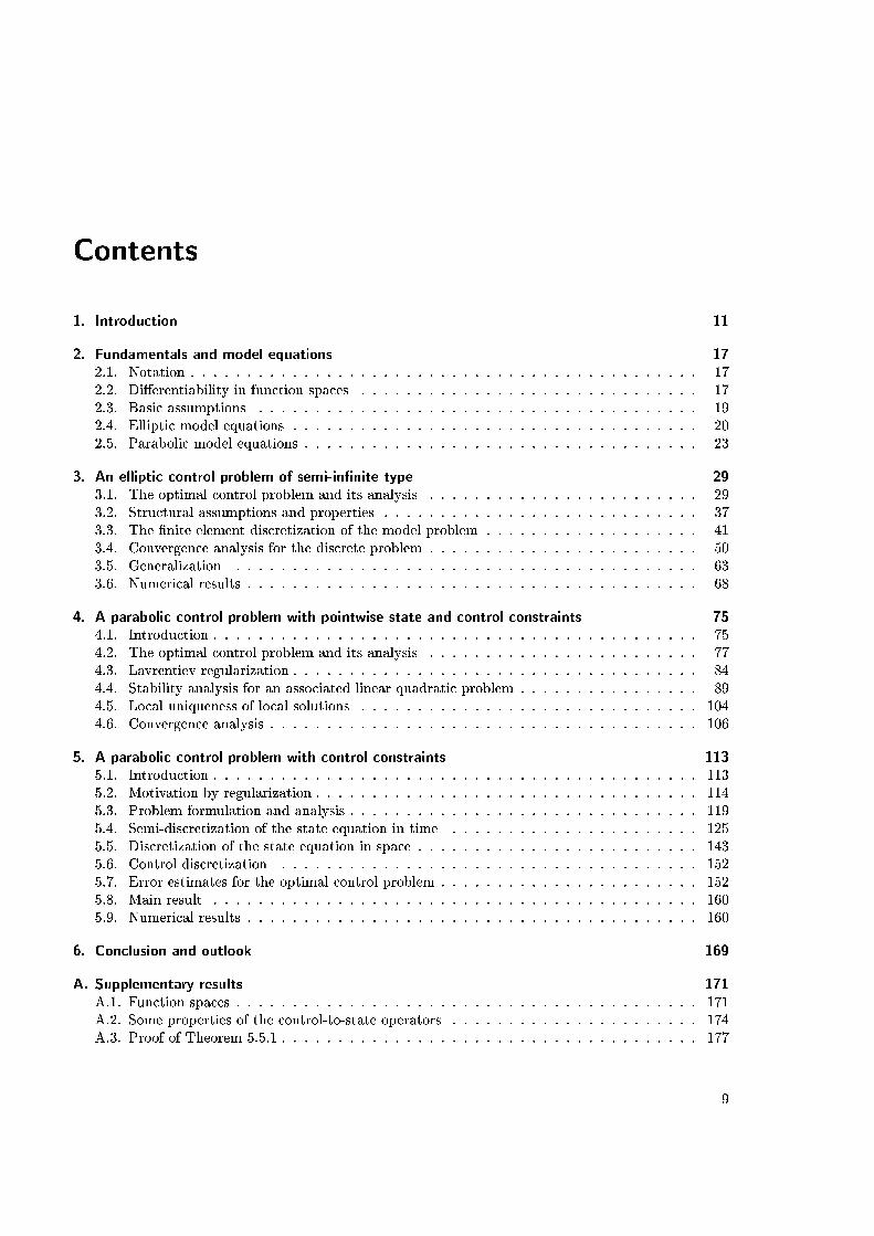
Contents
1. Introduction 11
2. Fundamentals and model equations 17
2.1. Notation . . . . . . . . . . . . . . . . . . . . . . . . . . . . . . . . . . . . . . . . . . . . . 172.2. Di�erentiability in function spaces . . . . . . . . . . . . . . . . . . . . . . . . . . . . . . 172.3. Basic assumptions . . . . . . . . . . . . . . . . . . . . . . . . . . . . . . . . . . . . . . . 192.4. Elliptic model equations . . . . . . . . . . . . . . . . . . . . . . . . . . . . . . . . . . . . 202.5. Parabolic model equations . . . . . . . . . . . . . . . . . . . . . . . . . . . . . . . . . . . 23
3. An elliptic control problem of semi-in�nite type 29
3.1. The optimal control problem and its analysis . . . . . . . . . . . . . . . . . . . . . . . . 293.2. Structural assumptions and properties . . . . . . . . . . . . . . . . . . . . . . . . . . . . 373.3. The �nite element discretization of the model problem . . . . . . . . . . . . . . . . . . . 413.4. Convergence analysis for the discrete problem . . . . . . . . . . . . . . . . . . . . . . . . 503.5. Generalization . . . . . . . . . . . . . . . . . . . . . . . . . . . . . . . . . . . . . . . . . 633.6. Numerical results . . . . . . . . . . . . . . . . . . . . . . . . . . . . . . . . . . . . . . . . 68
4. A parabolic control problem with pointwise state and control constraints 75
4.1. Introduction . . . . . . . . . . . . . . . . . . . . . . . . . . . . . . . . . . . . . . . . . . . 754.2. The optimal control problem and its analysis . . . . . . . . . . . . . . . . . . . . . . . . 774.3. Lavrentiev regularization . . . . . . . . . . . . . . . . . . . . . . . . . . . . . . . . . . . . 844.4. Stability analysis for an associated linear quadratic problem . . . . . . . . . . . . . . . . 894.5. Local uniqueness of local solutions . . . . . . . . . . . . . . . . . . . . . . . . . . . . . . 1044.6. Convergence analysis . . . . . . . . . . . . . . . . . . . . . . . . . . . . . . . . . . . . . . 106
5. A parabolic control problem with control constraints 113
5.1. Introduction . . . . . . . . . . . . . . . . . . . . . . . . . . . . . . . . . . . . . . . . . . . 1135.2. Motivation by regularization . . . . . . . . . . . . . . . . . . . . . . . . . . . . . . . . . . 1145.3. Problem formulation and analysis . . . . . . . . . . . . . . . . . . . . . . . . . . . . . . . 1195.4. Semi-discretization of the state equation in time . . . . . . . . . . . . . . . . . . . . . . 1255.5. Discretization of the state equation in space . . . . . . . . . . . . . . . . . . . . . . . . . 1435.6. Control discretization . . . . . . . . . . . . . . . . . . . . . . . . . . . . . . . . . . . . . 1525.7. Error estimates for the optimal control problem . . . . . . . . . . . . . . . . . . . . . . . 1525.8. Main result . . . . . . . . . . . . . . . . . . . . . . . . . . . . . . . . . . . . . . . . . . . 1605.9. Numerical results . . . . . . . . . . . . . . . . . . . . . . . . . . . . . . . . . . . . . . . . 160
6. Conclusion and outlook 169
A. Supplementary results 171
A.1. Function spaces . . . . . . . . . . . . . . . . . . . . . . . . . . . . . . . . . . . . . . . . . 171A.2. Some properties of the control-to-state operators . . . . . . . . . . . . . . . . . . . . . . 174A.3. Proof of Theorem 5.5.1 . . . . . . . . . . . . . . . . . . . . . . . . . . . . . . . . . . . . . 177
9
10 Contents
B. Notation 181
1. Introduction
The theory of optimal control of partial di�erential equations (PDEs) is a well-established �eld inapplied mathematics that developed rapidly along with the constant increase in computing power.Optimization problems that arise are widely spread, ranging from ow control, [64], over applicationsin material sciences such as optimal steel cooling or hardening strategies, cf. [43, 76], to applications inmedicine: in cancer therapy, for instance, the so-called local hyperthermia is employed to make tumorsmore susceptible for other forms of treatment, cf. [41], and optimal heating pro�les have to be developed.In these examples, the processes are governed by partial di�erential equations that are as diverse as theapplications themselves. Heat transfer equations, Maxwell's equation, or the Navier-Stokes equations,to name a few, may be encountered.
In general, a PDE constrained optimal control problem for a control u 2 U and a state y 2 Y for somecontrol space U and state space Y to be speci�ed takes the following abstract form:
Minimize J(y; u); subject to u 2 Uad; y = G(u);
whereJ = J(y; u) : Y � U ! R
is an objective functional that is to be minimized, and
G : U ! Y
denotes a so-called control to state mapping that in context of PDE constrained optimization involvesa solution operator of a partial di�erential equation. Each control u 2 U is assigned a unique statey = y(u) 2 Y . Finally, the set Uad is a set of admissible controls that handles additional constraintssuch as control bounds or pointwise constraints on the state. In the examples mentioned initially, theseconstraints are essential to obtain a meaningful problem formulation. For instance, in the steel coolingprocess the temperature di�erences in the steel must be bounded in order to avoid cracks, see [43]. Inlocal hyperthermia therapy, the generated temperature in the patient's body must not exceed a certainlimit, cf. [41].
A discussion of a general PDE-constrained optimal control problem includes the discussion of theunderlying PDE with respect to existence, uniqueness and regularity of solutions, the existence ofoptimal controls, as well as �rst order necessary and second order su�cient optimality conditions. Inaddition, adequate solution algorithms and discretization strategies have to be developed. And at last,it is desirable to estimate the quality of a discrete solution with the help of discretization error estimates.An introduction to these aspects can be found in the textbooks [144] or [74].
The analysis and even more so the development of e�cient numerical solution algorithms for PDEconstrained optimization problems became a vivid �eld in mathematics on the verge of functionalanalysis, optimization theory, and numerical mathematics. One of the founders of this theory is J. L.Lions, whose classical textbook [90] covers a wide-ranging theory for elliptic, parabolic, and hyperbolicoptimal control problems. However, up to today there remain interesting challenges, for instance with
11
12 1. Introduction
respect to problems with nonlinear state equation, the presence of pointwise state constraints, andaspects of numerical analysis not covered by [90]. Research projects like the DFG priority program1253 "Optimization with partial di�erential equations", are a public sign for this continued interest inthe topic.
This thesis is a contribution to the numerical analysis of PDE constrained optimal control problemsgoverned by semilinear elliptic and parabolic PDEs of heat equation type, subject to pointwise controland state constraints. We are especially interested in the discussion of pointwise state constraints, whichare known to lead to numerous theoretical and numerical di�culties. Let us give a brief overview aboutsome related questions and results.
One of the challenges related to pointwise state constraints lies within the formulation of �rst-orderoptimality conditions of Karush-Kuhn-Tucker-type (KKT) in useful spaces. This theory is often basedon the so called Slater condition, which we will state later. Then, the cone of non-negative functionsis required to have non-empty interior. This requires continuity of the state functions, because in Lp-spaces with 1 � p < 1 the cone of nonnegative functions has empty interior, while for p = 1 thedual space has very low regularity. Even if optimality conditions of Karush-Kuhn-Tucker-type can beformulated, the Lagrange multipliers associated with the pointwise state constraints are generally onlyobtained in the space of regular Borel measures, cf. [17], which in turn leads to low regularity of theadjoint state. We refer to e.g. further investigations by Casas, [18, 19], as well as Bergounioux andKunisch [11, 12], or Alibert and Raymond as well as Raymond and Zidani [2, 124, 125] for the discussionof pure pointwise state constraints.
Another di�culty is associated with second-order-su�cient conditions (SSC) for nonconvex problems,also a �eld of active research. There is quite a number of papers devoted to this subject. For PDE-constrained optimal control problems the �rst contributions are due to Tr�oltzsch and Goldberg, see[52, 53]. Further results involving state constraints have been obtained by Casas, Tr�oltzsch, and Unger,[28, 29] or Raymond and Tr�oltzsch, [123]. Yet, for parabolic problems in particular, the available theoryis not as general as desired. For spatio-temporal control functions for instance, and pointwise stateconstraints given in the whole domain Q, a satisfactory theory of SSC is so far only available for one-dimensional distributed control problems, cf. the recent results by Casas, de los Reyes, and Tr�oltzschin [22], or the earlier works by Raymond and Tr�oltzsch, [123]. Only in special cases, i.e. a setting with�nitely many time-dependent controls, SSC have been shown to hold for higher dimensions by de losReyes, Merino, Rehberg and Tr�oltzsch, cf. [36].
These theoretical challenges also in uence the numerical analysis of optimal control problems, for in-stance when trying to derive a priori discretization error estimates. There is a number of publicationson elliptic control-constrained optimal control problems, [8, 21, 25, 26, 27, 37, 71, 82, 109, 130], derivingerror estimates for boundary and distributed control problems with di�erent types of control discretiza-tion, for problems with linear and semilinear state equation. Fewer results are known for problemswith pointwise state constraints in the whole domain. Here, we mention the convergence results byCasas in [20] for problems with �nitely many state constraints, and the error estimates for ellipticstate constrained distributed control functions by Casas and Mateos in [23], Deckelnick and Hinze in[38, 39] and Meyer in [107]. We will give a more detailed overview in Chapter 3. Further results involv-ing gradient constraints where obtained by G�unther and Hinze in [63] and Ortner and Wollner, [119].Recently, some progress with respect to optimal error estimates has been made for state-constrainedelliptic problems with �nite dimensional control space. In [106], Merino, Vexler and Tr�oltzsch analyzeda problem with �nitely many pointwise state constraints and derived error estimates that re ect theerror for uncontrolled equations. Then, in [104] and [105] linear quadratic problems of semi-in�nitetype, i.e. with �nite dimensional control space and pointwise state constraints in a domain have beenanalyzed by Merino, Tr�oltzsch, and the author, where the same order of convergence is proven under
13
certain conditions. Comparable results for nonconvex problems with semilinear state equation will bepresented in this thesis.
For parabolic optimal control problems, the situation is even more di�cult. Even for parabolic control-constrained problems the theory is not as developed as in the elliptic setting. There are a number ofcontributions to the analysis of linear-quadratic problems. A fundamental contribution certainly comesfrom Malanowski, [92], where error estimates for the control are proven for Galerkin-type approxima-tions of convex control-constrained parabolic problems. In [101, 102], Meidner and Vexler derived errorestimates for the control utilizing discontinuous Galerkin schemes that clearly separate the in uenceof spatial and temporal discretization. We refer also to [87, 129, 150, 103] for further investigations.For nonconvex problems, we mention also the early results of McNight and Bosarge, jr., [98], where aLagrange multiplier approach has been used. For control-constrained problems with semilinear stateequation, we refer to Chrysa�nos' results on plain convergence in [33], and to the recent publication ofVexler and the author, cf. [118], for �nite element error estimates, extending the linear-quadratic settingfrom [102]. Only very few attempts have been made to derive a priori error estimates for the �niteelement discretization of parabolic state constrained optimal control problems. To the author's knowl-edge, there are only two contributions for linear-quadratic problems. Deckelnick and Hinze consideredthe variational discretization for �nitely many time-dependent controls, cf. [40]; and linear-quadraticproblems with pointwise-in-time state constraints have been discussed by Meidner, Rannacher, andVexler in [100].
For all these reasons, regularization techniques have been a wide �eld of active research in the recentpast and remain to be of interest. We mention for example a Moreau-Yosida regularization approachby Ito and Kunisch, [78], a Lavrentiev-regularization technique by Meyer, R�osch, and Tr�oltzsch, [110],or for boundary control problems the source-term representation-based Lavrentiev regularization byTr�oltzsch and Yousept, [145], or Tr�oltzsch and the author, [116], as well as the virtual control conceptby Krumbiegel and R�osch, [85]. Moreover, barrier methods, have regularizing e�ect. We will not discussthese methods in this thesis, but we refer for instance to Schiela, [135], Pr�ufert et. al. [121] or Ulbrichand Ulbrich, [147].
All mentioned types of regularization have been subject to further intensive research. The main interestlies again in the discussion of optimality conditions, but also on convergence issues and estimation ofthe regularization error. In addition, the question of convergence of solution algorithms is of interest ifa problem is to be solved numerically. Then, estimating the discretization error of regularized problemsis also desirable.
For Moreau-Yosida related publications, we refer for instance to Bergounioux, Haddou, Hinterm�ullerand Kunisch, [10], Bergounioux and Kunisch, [12], Hinterm�uller, Ito, and Kunisch, [66], Hinterm�ullerand Kunisch, [67], and Hinterm�uller, Tr�oltzsch and Yousept, [69], to name a few. Recent resultsby Hinterm�uller and Kunisch, [68], take into account not only control and state constraints but alsoconstraints on the derivative. We also point out [112], where Meyer and Yousept derived convergence fora nonconvex elliptic problem and to [115] for parabolic convergence results for problems with semilinearstate equation derived by Tr�oltzsch and the author.
Meanwhile, Lavrentiev regularization has also attracted much attention. Numerical methods, theoreticalproperties, and di�erent problem formulations have been investigated. We refer to results by Tr�oltzschet. al. in [120, 142] for linear-quadratic problems, [111] for semilinear elliptic problems, the discussionof second order su�cient conditions by R�osch and Tr�oltzsch in [131, 132], and further investigationsby R�osch et. al., [30, 31] as well as Griesse et. al., [61, 60], for the discussion of solution algorithms.Closely related are also problems with constraints of bottleneck type, cf. the analysis of such problemsby Bergounioux and Tr�oltzsch, [13, 14]. A challenge posed by a so called fully constrained problem with
14 1. Introduction
lower and upper mixed control-state constraints as well as box constraints concerning the existence ofLagrange multipliers has been solved by R�osch and Tr�oltzsch in [132]. Linear-quadratic fully constrainedparabolic problems have been investigated in [116] by Tr�oltzsch and the author, including a discussionof boundary control problems motivated by the benchmark problem by Betts and Campbell, cf. [15].Convergence and error estimates for parabolic problems governed by semilinear equations have to theauthor's knowledge only been studied in [115].
Finite element error estimates for regularized problems are also of interest. Elliptic problems withregularized pointwise state constraints have been discussed mainly by Hinze et. al., [73], and R�oschet. al. in [32]. The discretization for interior point methods in the presence of pointwise state constraintshas been analyzed in [75], and the discretization of Moreau-Yosida regularization is discussed in [65].
In this thesis, we will aim at closing some of the remaining gaps in the theory of PDE-constrainedoptimal control problems subject to pointwise inequality constraints. The motivating question is thedevelopment of a priori-error estimates for the �nite element discretization of state-constrained optimalcontrol problems, subject to semilinear elliptic and parabolic heat equations. We will address di�erentaspects. Throughout, we are interested in analyzing local solutions of nonconvex problems. After ashort introduction into fundamental regularity theory for the underlying partial di�erential equationsin Chapter 2 we will address three main topics:
� We will discuss an elliptic state constrained problem of semi-in�nite type in Chapter 3. Thecomparably high regularity of solutions to semilinear elliptic state equations, the rather simplecontrol-structure of only �nitely many control parameters, and readily available discretizationerror estimates for uncontrolled equations in two space dimensions allows to focus entirely on thechallenges of pointwise state constraints. Under some assumptions to be discussed, involving inparticular an assumption on the active set that allows to characterize the structure of the Lagrangemultipliers, we prove a convergence result for discrete optimal controls that re ects the convergenceorder of uncontrolled equations. The main ideas applied in this section have been published byMerino, Tr�oltzsch, and the author in [104] and [105] for linear-quadratic problems. Additionally,we have to take into account the di�culties posed by nonconvex problem formulations, such asconvergence of local solutions, quadratic growth conditions, and facts as simple as not having asuperposition principle for nonlinear state equations. We will conduct some numerical tests, butthe discussion of e�cient solution algorithms shall not be the purpose of this chapter. Therefore,we simply revert to available nonlinear programming solvers for the completely discretized problemformulations.
� In principle, we are also interested in �nite element error estimates for parabolic state constrainedproblems, where we look at problems with distributed control functions that can vary arbitrarilyin space and time. This problem class unites numerous di�culties, from more restrictive regularityresults for parabolic equations, to the fact that in general the active sets are di�cult to charac-terize, to the challenge of having to develop error estimates in space and time, depending on twoessentially di�erent discretization parameters. We will therefore consider a Lavrentiev regularizedversion of a parabolic control-and-state constrained optimal control problem. In Chapter 4, onekey issue will be to provide a convergence result for Lavrentiev parameter tending to zero, as wellas a regularization error estimate. Secondly, we dwell on the improved regularity properties ofthe regularized problem, and discuss properties of the regularized problem including second-ordersu�cient optimality conditions and a stability analysis of associated linear-quadratic problems,that in particular give rise to a local uniqueness result and may also be used for a convergencediscussion of numerical solution algorithms. In contrast to the discussion of comparable ellip-tic problems, we have to take into account the fact that L2-controls do not in general generatebounded states, which complicates the analysis in several points. Most of the results presented
15
in Chapter 4 have been published by Tr�oltzsch and the author in [115]. See also [114] for a shortoverview.
� Then, in Chapter 5, we develop a priori error estimates for the �nite element discretization ofcontrol-constrained optimal control problems governed by a semilinear parabolic state equation.While the results of Chapter 5 are interesting in their own right, we also motivate how under certainassumptions the model problem can be interpreted as a Lavrentiev-regularized version of a state-constrained model problem, cf. [73] for a similar elliptic setting, and in that sense also complementsthe study of state-constrained model problems. We give some results on regularization that havebeen proven and published for linear-quadratic problems by Tr�oltzsch and the author in [116]. Theresults on error estimates presented in this chapter have been published by Vexler and the authorin [118] for a slightly di�erent objective function. The extension to the more general problemformulation is straight-forward, but necessary in order to discuss certain Lavrentiev-regularizedproblems.
A brief overview about the �rst two items can also be found in [117].
Before we turn to the detailed analysis of the mentioned example problems, let us say a few wordsabout the notation used. In the next chapter, we will agree on some general underlying assumptionsand notation, but in the interest of readability, the notation will only be completely consistent chapterby chapter. In particular, the same name may be used for similar but not necessarily identical things.For instance, the control-to-state operator associated with the nonlinear state equations will always bedenoted by G. Since the main chapters are self-contained, this will be no cause of confusion. The onlyoverlap will appear between Chapters 4 and 5 when it comes to the properties of G, but it will beimmediately apparent that the properties of G proven in Chapter 4 transfer to Chapter 5. Last, let usmention that the �rst section of each of the Chapters 3-5 contains a short introduction to the modelproblem and a summary of known results as a bene�t for the reader, since most of these properties areused in the following analysis.

2. Fundamentals and model equations
Naturally, existence and regularity issues of the governing PDE play an important role for a thoroughanalysis of PDE-constrained optimal control problems. For that reason, we begin this thesis with apresentation of some functional analytic basics and known existence and regularity results for the PDEsunder consideration. For further information we point out textbooks on functional analysis, e.g. [1],partial di�erential equations, e.g. [48], or optimal control, [144].
2.1. Notation
For the solution theory of both elliptic and parabolic partial di�erential equations we require certainregularity assumptions on the involved spatial domain � Rn, n 2 N. Note �rst that the term domainautomatically implies that is an open and connected set. Throughout, we will work with convexLipschitz domains, e.g. domains whose boundary � := @ can locally be expressed as the graph ofa Lipschitz continuous function. We refer to e.g. [113] for a more detailed characterization of domainsand their boundaries. An important class are polygonally or polyhedrally bounded convex domains inR2 or R3.
We use standard notation for the Lebesgue spaces Lp(), Sobolev spaces Wm;p(), with the short no-tation Hm() :=Wm;2(), as well as some spaces of continuous functions, including H�older continuousfunctions. For time-dependent problems, we will make use of spaces of abstract functions, or vectorvalued functions, that are de�ned on a compact time interval and admit values in Banach spaces. Werefer the reader to Appendix A.1 for a short overview, and to standard monographs such as [1] for adetailed discussion. Details can also be found in [144], where functional analytic fundamentals that areapplied in optimal control are presented in a concise way.
2.2. Di�erentiability in function spaces
For each model problem under consideration, we will review �rst and second-order optimality conditions.This involves some kind of di�erentiation of what we will call a control-to-state mapping, as well as theobjective function. We state precise de�nitions and conditions collected in [144].
De�nition 2.2.1. Let fU; k � kUg; fW; k � kW g be normed linear spaces. A mapping T : U � U !W issaid to be Fr�echet di�erentiable at u 2 U if there exists an operator T 0(u) 2 L(U;W ) and a mappingr(u; �) : U !W with the following properties: for all v 2 U such that u+ v 2 U , we have
T (u+ v) = T (u) + T 0(u)v + r(u; v);
where r satis�es the conditionkr(u; v)kWkvkU ! 0 as kvkU ! 0:
17

18 2. Fundamentals and model equations
The operator T 0(u) is then called the Fr�echet derivative of T at u. T is said to be continuously Fr�echetdi�erentiable if
ku� vkU ! 0 ) kT 0(u)� T 0(v)kL(U;W ) ! 0
is satis�ed.
For a continuous linear operator T , di�erentiability is easily obtained and T 0(u) = T for all u is observed.However, our model problems are governed by certain types of nonlinearities, both in the PDE itselfand in the objective function. These nonlinearities depend on either or both the control u and the statey. The arising operators are called superposition operators, or Nemytskii operators. We give a shortoverview about their properties, and refer to [81] or again to [144] for more details.
De�nition 2.2.2. Let E � Rn, n 2 N, be a bounded set, and let � = �(e; �) : E � Rm ! R, m 2 N bea function. The mapping � given by
�(�) = �(�; �(�));which assigns to a (possibly vector valued) function � : E ! Rm the function � : E ! R, �(e) =�(e; �(e)), is called a Nemytskii operator.
We will assume the following Carath�eodory-type, boundedness, and Lipschitz continuity conditions oforder two for the de�ning nonlinearity �:
Assumption 2.2.3. The function � = �(e; �) : E � Rm ! R is measurable with respect to e 2 E forall �xed � 2 Rm, and twice continuously di�erentiable with respect to � for almost all e 2 E. For � = 0,it is bounded of order two with respect to e by a constant K > 0, i.e. � is assumed to satisfy
j�(�; 0)j+ j�0(�; 0)j+ j�00(�; 0)j � K; (2.2.1)
where �0 and �00 denote the �rst and second order derivative of � with respect to �. Also, � and itsderivatives with respect to � up to order two are uniformly Lipschitz on bounded sets, i.e. for all S > 0there exists LS > 0 such that � satis�es
j�00(�; �1)� �00(�; �2)j � LS j�1 � �2j (2.2.2)
for all �i 2 Rm with j�ij � S.
In the last assumption and throughout the following,
j � j; and h�; �idenote the norm and inner product in Rm, respectively. We will use this for instance for elements x 2 as well as u 2 Rm. For brevity of notation, we will also use j � j as a matrix norm for e.g. �00. Later on,we will replace E by a spatial domain or a space-time domain Q, with elements e = x, or e = (t; x),respectively. Moreover, � 2 Rm will be replaced by y or (y; u). Under these assumptions, it is knownthat the Nemytskii operator � is continuous in L1(E), and locally Lipschitz continuous with respectto the Lr(E) norm for every 1 � r � 1. Moreover, � is continuously Fr�echet di�erentiable in L1(E),with derivative
(�0(�)v)(e) = �0(e; �(e))v(e)
for all v 2 L1(E) and almost all e 2 E, where �0 denotes the derivative of � with respect to �. Forconsideration of other Lp-spaces, note that �(�) maps Lp(E)m into Lq(E) for 1 � q � p < 1 if andonly if there are functions � 2 Lq(E) and � 2 L1(E) such that the growth condition
j�(e; �)j � �(e) + �(e)j�j pq

2.3. Basic assumptions 19
is satis�ed. Then, � is automatically continuous for q <1. It is di�erentiable from Lp(E) into Lq(E),if the Nemytskii operator generated by �0(e; �) maps Lp(E) into Lr(E) with
r =pq
p� q:
This will turn out useful when discussing di�erent types of objective functionals, and second ordersu�cient conditions. For more details, we refer to [144, Chapter 4], and the references mentionedtherein.
2.3. Basic assumptions
Due to the diverse nature of the model problems considered we will have to specify some assumptionsand convenient notation chapter by chapter. There are, however, some fundamental assumptions thatcan be formulated for all what follows.
Assumption 2.3.1. Let � Rn, 1 � n � 3, be a nonempty convex Lipschitz domain with boundary� := @ if n > 1, or a bounded interval for n = 1. For a time dependent problem, we denote byI := (0; T ) a time interval with �xed �nal time T > 0, and Q := I � denotes the space-time-domainwith boundary � := I � �.
As a rule of thumb, our results on discretization will be con�ned to two space dimensions due either toerror estimates for uncontrolled equations that are only readily availabe in 2D, or to the regularity ofthe discrete solutions themselves.
We will basically consider two types of state equations, the semilinear elliptic boundary value problem
Ay + d(x; y; u) = 0 in ;y = 0 on �;
(2.3.1)
where u 2 Rm is a vector of control parameters, and its parabolic analogue
@ty +Ay + d(t; x; y) = u in Q;y(0; �) = y0 in ;
y = 0 on �;(2.3.2)
for space-time-dependent control functions u with regularity yet to be discussed. Note that in (2.3.1),where u is a vector of real numbers, we allow d to depend on u. Both PDEs are governed by a uniformlyelliptic and symmetric di�erential operator A, de�ned by
Ay(x) = �nX
i;j=1
@j(aij(x)@iy(x)) (2.3.3)
with coe�cients aij 2 C0;1+�(); 0 < � < 1, that satisfy
m0j�j2 �nX
i;j=1
aij(x)�i�j 8� 2 Rn; a.e. in (2.3.4)
for some m0 > 0. Moreover, @ty denotes the partial derivative of y with respect to time. We point outthat the choice of homogeneous Dirichlet boundary conditions is mostly due to a uni�ed presentation of
20 2. Fundamentals and model equations
results. The theory can be adapted to homogeneous variational boundary conditions as long as unique-ness of solutions is guaranteed in the elliptic setting, but then Poincar�e's inequality is not applicableand some proofs become more involved. The results on regularization presented in Chapter 4 transferalso to inhomogeneous Robin-type boundary conditions with su�ciently regular boundary data.
Later on, we will refer to u as the control and to y as the state. For now, let us discuss the existence andregularity of solutions to (2.3.1) and (2.3.2) for �xed u from a respective appropriate control space.
2.4. Elliptic model equations
We �rst discuss existence and regularity of solutions of the uncontrolled elliptic state equation (2.3.1) aswell as linear equations as they will later on appear as adjoint equations or linearized state equations.Therefore, we de�ne the control space
U := Rm;
and consider a �xed u 2 Rm throughout this section. The canonical state space will be the space H10 (),
and we introduce the short notationV := H1
0 ():
However, H1-regularity will not be su�cient for our purposes, since we will consider pointwise stateconstraints in our model problem formulation. We will therefore provide higher regularity results.Throughout, we use the following abbreviations for the inner product and norm on L2():
(�; �) := (�; �)L2(); k � k := k � kL2():Moreover, for the norms on Lp() with 1 � p < 1 and especially for the L1()-norm we use theabbreviations
k � kp := k � kLp(); k � k1 := k � kL1():
In addition, for a real number � > 0 and an element x 2 we de�ne B�(x) to be the open ball in Rn
around x with radius �. If instead of x 2 a control vector u 2 Rm is given, then B�(u) denotes theopen ball in Rm around u.
Let �rst the linear elliptic boundary value problem
Ay + d0y = f in ;y = 0 on �
(2.4.1)
with data f 2 L2() and d0 2 L1(), d0 � 0 be given. It is reasonable to look for solutions in weaksense, since the homogeneous Dirichlet boundary conditions do not require i.e. very weak solutionconcepts. For the convenient discussion of elliptic PDEs, we de�ne the bilinear form
a : V � V ! R; a(v; w) =
nXi;j=1
(aij@iv; @jw):
Note that we do not include the term associated with d0 in the bilinear form a, since this will leave more exibility to use a also for e.g. linearized equations when combining it with an appropriate additionalterm.
De�nition 2.4.1. A function y 2 H10 () is said to be a weak solution of the Dirichlet problem (2.4.1)
if it ful�llsa(y; ') + (d0y; ') = (f; ') 8 ' 2 H1
0 ():

2.4. Elliptic model equations 21
Proposition 2.4.2. Let Assumption 2.3.1 be satis�ed and let 1 be a subdomain of with �1 � .For every right-hand side f 2 L2(), the linear boundary value problem (2.4.1) admits a unique weaksolution y 2 H1
0 (). Moreover, the solution exhibits the improved regularity
y 2 H10 () \H2() \ C(�);
and there exists a constant C > 0 not depending on f , such that the estimate
kyk+ kryk+ kr2yk+ kykC(�) � C kfk
is satis�ed. For f 2 C0;� with a real number � 2 (0; 1), we even have
y 2 C2;�() \W 2;1(1):
Proof. The existence and uniqueness of y 2 H10 () is a standard result, following from the Lax-Milgram
lemma after applying Poincar�e's inequality. Since we assume to be a bounded, convex Lipschitzdomain, Theorem 3.2.1.2 in [62] guarantees a solution y 2 H2(). By a Sobolev embedding theorem,cf. e.g. [1], we obtain continuity of the solution by n � 3. The C2;�-regularity follows directly from[51, Theorem 6.13] noting that convex polygonal domains ful�ll a so-called exterior sphere condition,i.e. for each x� 2 �, there exists a sphere B = B�(y) satisfying �B \ � = x�. From C2;�-regularity on�1 � the desired W 2;1-regularity on 1 is immediately obtained.
We also point out the results in [2] and [18], where boundedness and continuity of solutions havebeen discussed for Neumann boundary value problems in n-dimensional domains for right-hand sidesf 2 Lp(), p > n=2. Applying results by Griepentrog, cf. [56], continuity is also obtained under weakerregularity assumptions on the coe�cients of the di�erential operator.
Finally, before turning to the nonlinear equation, we present an existence and regularity result for linearelliptic Dirichlet problems with an element � 2 C()� in the right-hand side. In the sequel, we identifyC()� with the set of regular Borel measures M(), cf. [3]. We will encounter this type of equationwhen deriving �rst order optimality conditions for the semi-in�nite optimal control problem in Chapter3. Elliptic problems with mixed boundary conditions and measures in the right-hand side as well as inthe boundary term have been discussed by Casas, cf. [18], and Alibert and Raymond, [2]. A problemwith A = �� and homogeneous Dirichlet boundary conditions on smooth domains is discussed in detailin Section 5.3.5 of [16]. We consider the boundary value problem
Ap+ d0p = � in ;p = 0 on �:
(2.4.2)
We follow Casas, [17], and call p 2 L2() a solution of (2.4.2), if and only ifZ
(�nX
i;j=1
@j(aij(x)@i'(x)) + d0')(x)p(x)dx =
Z
'(x)d�(x); 8 ' 2 H2() \H10 () (2.4.3)
is satis�ed.
Proposition 2.4.3. Let Assumptions 2.3.1 be true and let d0 2 L1() be a given nonnegative function.For every � 2 C0()�, the boundary value problem (2.4.2) admits a unique solution p 2W 1;s
0 () for alls 2 [1; n=(n� 1)), and there exists a constant C = C(s) > 0 such that
kpkW 1;s0 () � Ck�kC()� :
22 2. Fundamentals and model equations
Proof. This follows from [17].
The homogeneous Dirichlet boundary conditions will later be motivated by prescribing state constraintsonly in the interior of . Now, we consider the nonlinear state equation (2.3.1), where we rely on thefollowing precise setting of Assumption 2.2.3.
Assumption 2.4.4. In (2.3.1), the function d = d(x; y; u) : � R � Rm ! R is H�older continuouswith respect to x 2 for all �xed (y; u) 2 R�Rm, and twice continuously di�erentiable with respect to(y; u) for all x 2 . For y = u = 0, it is bounded of order two with respect to x by a constant K > 0,i.e. d is assumed to satisfy
jd(�; 0; 0)j+ jd0(�; 0; 0)j+ jd00(�; 0; 0)j � K; (2.4.4)
where d0 and d00 denote the �rst and second order derivative of d with respect to (y; u). Also, d and itsderivatives with respect to (y; u) up to order two are uniformly Lipschitz on bounded sets, i.e. for allS > 0 there exists LS > 0 such that d satis�es
jd00(�; y1; u1)� d00(�; y2; u2)j � LS(jy1 � y2j+ ju1 � u2j) (2.4.5)
for all yi; ui 2 R with jyij; juij � S. Moreover, d is monotone with respect to y, i.e. suppose that@yd(�; y; u) > 0.
De�nition 2.4.5. For a given control vector u 2 Rm, a function y 2 H10 () is said to be a weak
solution of the Dirichlet problem (2.3.1) if it ful�lls
a(y; ') + (d0y; ') + (d(�; y; u); ') = 0 8 ' 2 H10 ():
We obtain an existence and regularity result similar to the linear setting.
Theorem 2.4.6. Let Assumptions 2.3.1 and 2.4.4 hold and let 1 be a subdomain of with �1 � .For each control u 2 Rm, there exists a unique weak solution
y 2 H10 () \H2() \ C(�) \ C2;�() \W 2;1(1)
of (2.3.1). We obtain the existence of a positive constant C, such that
kyk+ kryk+ kr2yk+ kykC(�) + kykW 2;1(1) � C(juj+ 1):
Proof. The existence of a unique solution y 2 H1()\L1() follows from similar arguments as in [144],where a semilinear problem with Neumann boundary conditions has been discussed. As a preliminarystep, assume that the nonlinearity d is globally bounded, and apply the steps of [144, Theorem 4.5],which are based on a method by Stampacchia, cf. [80], to
Ay + d(�; y; u)� d(�; 0; u) = �d(�; 0; u) in ;y = 0 on �:
Here, the monotonicity of d with respect to y can be used when testing the weak formulation with y.Due to the Lipschitz properties of d, it is clear that eventually the right-hand side can be estimated by
kd(�; 0; u)k � kd(�; 0; u)� d(�; 0; 0)k+ kd(�; 0; 0)k � c(juj+ 1):
2.5. Parabolic model equations 23
By applying a cut-o� argument from Casas, [18], to the possibly unbounded nonlinearity d one obtainsthe existence of a solution y 2 H1
0 () \ L1() satisfying the estimate
kykH10 ()
+ kykC(�) � C(juj+ 1);
taking advantage of the monotonicity and Lipschitz continuity of d. The remaining estimates follow byapplying Proposition 2.4.2 to the linear equation
Ay = �d(�; y; u) in ;y = 0 on �;
since under Assumption 2.4.4 we have d(�; y; u) 2 C0;�(). We refer also to the proof of Lemma 3 in[106].
2.5. Parabolic model equations
We will now build the basis for the further analysis of the parabolic model problems. Throughout thefollowing, it will be helpful to make use of a short notation for inner products and norms on the spacesL2(Q) and L1(Q):
(v; w)I := (v; w)L2(Q); kvkI := kvkL2(Q); kvk1;1 := kvkL1(Q): (2.5.1)
The subscript I is motivated by the notation for the time interval I, and will prove to be more legiblethan e.g. a subscript Q. In some estimates, we will also need the norm
kvk1;2 := kvkL1(I;L2()):
We still use the short notationV := H1
0 ();
and note that by identifying the space H := L2(Q) with its dual space H� we have a Gelfand triple
V ,! H �= H� ,! V �;
where the embeddings are dense, compact, and continuous. Moreover, we de�ne
Y :=W(0; T ) = fy j y 2 L2(I; V ) and @ty 2 L2(I; V �)g:For future reference, we point out that the embedding W(0; T ) ,! L2(Q) is compact, cf. for instance[89]. Then, let the parabolic initial-boundary value problem
@ty +Ay + d0y = f in Q;y(0; �) = y0 in ;
y = 0 on �(2.5.2)
be given with data f 2 L2(Q), y0 2 V and d0 2 L1(Q).
De�nition 2.5.1. A function y 2 W(0; T ) is called a weak solution of (2.5.2) if it ful�lls
TR0
h@ty; 'iV �;V dt+RRQ
nPi;j=1
aij@iy@j' dxdt;+RRQ
d0y' dxdt =RRQ
f' dxdt 8 ' 2 L2(I; V )
y(0; �) = y0 in ;
where h�; �; iV �;V denotes the duality pairing between V � and V .

24 2. Fundamentals and model equations
We will provide an existence result for solutions of the linear equation in the state space Y: We willalso provide higher regularity of the solution depending on the given data. On the one hand, we areinterested in continuity, to eventually derive a continuity result for the nonlinear state equation whichwe will need to discuss state constraints appropriately. On the other hand, we will need a higherregularity result for the derivative with respect to time, as well as an estimate for the second orderspatial derivative in order to derive discretization error estimates.
Proposition 2.5.2. Let Assumption 2.3.1 hold and let d0 2 L1(Q) be given. For every functionf 2 L2(Q) and initial state y0 2 L2(), the initial boundary value problem (2.5.2) admits a uniquesolution y 2 W(0; T ). In addition, the estimate
kykI + kyk1;2 + kykW(0;T ) � C (kfkI + ky0k)
is ful�lled for a constant C > 0. If the initial state admits the regularity y0 2 V , y exhibits the improvedregularity
y 2 L2(I;H2() \ V ) \ L1(I; V ) \H1(I; L2());
and the estimate
kryk1;2 + kr2ykI + k@tykI � C (kfkI + ky0kV )is satis�ed. For f 2 Lp(), p > n=2 + 1 and y0 2 C(�); y belongs to C( �Q), and the estimate
kykC( �Q) � C(p)(kfkLp(Q) + ky0kC(�))
is satis�ed.
Proof. For the existence of a unique solution y 2 W(0; T ) we refer to [86], or [144] for homogeneousvariational boundary conditions. The main idea is to �rst consider a weak formulation of the initialboundary value problem with test functions ' 2 H1(I; L2())\L2(I; V ), that satisfy '(�; T ) = 0. Theexistence of a unique weak solution y 2 L2(I; V ) is obtained by a Galerkin approximation and is provento be a function from W(0; T ). Cf. also [90] or [151]. The continuity result is proven in [144] forRobin-type boundary conditions based on results on maximal parabolic regularity for problems withzero initial state from [57, 58], which also hold for homogeneous Dirichlet boundary conditions. Finally,the regularity
y 2 L2(I;H2() \ V ) \ L1(I; V ) \H1(I; L2())
is proven in [48].
Boundedness in the norm k�k1;1 is obviously also obtained. For that result, we require the initial statey0 to be bounded, only. Continuity of solutions was also discussed by Casas in [19], or by Raymondand Zidani, cf. [125].
The semilinear equation (2.3.2) is discussed next, under assumptions on the nonlinearity d that �t intothe setting of Assumption 2.2.3.
Assumption 2.5.3. In (2.3.2), the function d = d(t; x; y) : Q � R ! R is measurable with respect to(t; x) 2 Q for all �xed y 2 R, and twice continuously di�erentiable with respect to y for almost all(t; x) 2 Q. For y = 0, it is bounded of order two with respect to (t; x) by a constant K > 0, i.e. d isassumed to satisfy
jd(�; 0)j+ jd0(�; 0)j+ jd00(�; 0)j � K; (2.5.3)

2.5. Parabolic model equations 25
where d0 and d00 denote the �rst and second order derivative of d with respect to y. Also, d and itsderivatives with respect to y up to order two are uniformly Lipschitz on bounded sets, i.e. for all S > 0there exists LS > 0 such that d satis�es
jd00(�; y1)� d00(�; y2)j � LS jy1 � y2j (2.5.4)
for all yi 2 R with jyij � S. Last, suppose that @yd(�; y) > 0.
A weak formulation is given in the following de�nition.
De�nition 2.5.4. A function y 2 W(0; T ) is a weak solution of (2.3.2) if it ful�lls
TR0
h@ty; 'iV �;V dt+RRQ
nPi;j=1
aij@iy@j' dxdt;+RRQ
d(�; y)'dxdt = RRQ
f' dxdt 8' 2 L2(I; V )
y(0; �) = y0 in :
If data in L2-spaces is given, the following theorem provides solvability of the nonlinear initial-boundaryvalue problem in useful spaces, yet relying on more restrictive assumptions on the nonlinearity.
Theorem 2.5.5. Let Assumption 4.2.1 hold with global boundedness and Lipschitz properties of d,i.e. the properties formulated in Assumption 2.2.3 hold for all y 2 R. For every function f 2 L2(Q),and initial state y0 2 L2(), the initial boundary value problem (5.2.1b) admits a unique solutiony 2 W(0; T ), and the estimate
kykW(0;T ) � C(kfkI + ky0k+ 1)
holds for a constant C > 0. In addition, if y0 2 V , the solution exhibits the improved regularity
y 2 L2(I;H2() \ V ) \ L1(I; V ) \H1(I; L2()) ,! C(�I; V )and the estimate
kykL1(I;V ) + kykL2(I;H2()) + k@tykI � C(kfkI + ky0kV + 1)
is ful�lled for a constant c > 0.
Proof. Existence of such a solution is obtained by a Galerkin method, taking into account appropriateconvergence results to cope with the nonlinearity. For the complete proof, we refer e.g. to [144] for ananalogous problem with Robin-type boundary condition. An essential ingredient is the monotonicity ofd. Adding the term �d(�; 0) to both sides of (2.3.2) and noting that
(d(�; y)� d(�; 0); y)I � 0
eventually yields the estimate
kyk1;2 + kykW(0;T ) � kfkI + kd(�; 0)kI ;which explains the term +1 in the a priori estimate. The higher regularity of y then follows fromapplying Proposition 2.5.2 to the linear equation
@ty +Ay = f � d(�; y) in Qy(0; �) = y0 in
y = 0 on �;
estimating
kd(�; y)kLp(Q) � kd(�; y)� d(�; 0)kLp(Q) + kd(�; 0)kLp(Q) � LkykLp(Q) + kd(�; 0)kLp(Q)
by the Lipschitz continuity of d, if d is globally Lipschitz continuous.
26 2. Fundamentals and model equations
For higher regularity of the given data we obtain the following existence and regularity result underweaker assumptions on the nonlinearity:
Theorem 2.5.6. Let Assumptions 2.3.1 and 2.4.4 hold. For every function f 2 Lp(Q), p > n=2 + 1,and initial state y0 2 C0(�), the initial boundary value problem (2.5.2) admits a unique solution y 2W(0; T ) \ C( �Q), and the estimates
kykC( �Q) � C (kfkLp(Q) + ky0kC(�) + 1);
kykI + kyk1;2 + kykW(0;T ) � C (kfkI + ky0k+ 1)
hold for a constant C > 0. In addition, if y0 2 V , the solution exhibits the improved regularity
y 2 L2(I;H2() \ V ) \ L1(I; V ) \H1(I; L2()) ,! C(�I; V )
and the estimate
krykI + kryk1;2 + kr2ykI + k@tykI � C (kfkI + ky0kV + 1)
is ful�lled for a constant C > 0.
Proof. Existence and continuity of a solution y is shown in [144] for mixed boundary conditions. Ina �rst step, the existence of a solution in W(0; T ) under stronger assumptions on the nonlinearity d,i.e. global boundedness and Lipschitz continuity, is shown for data in L2-spaces, cf. Theorem 2.5.5. Acut-o� argument applied to a possibly unbounded nonlinearity d shows boundedness of the solutions ifthe data is regular enough. We refer to [144] and the references therein for details. The higher regularityof y, including continuity, follows again by applying Proposition 2.5.2 to the linear equation
@ty +Ay = f � d(�; y) in Qy(0; �) = y0 in
y = 0 on �;
estimating
kd(�; y)kLp(Q) � kd(�; y)� d(�; 0)kLp(Q) + kd(�; 0)kLp(Q) � LkykLp(Q) + kd(�; 0)kLp(Q):
Here, local Lipschitz continuity of d is su�cient since y is already known to be bounded.
Again, if y0 2 L1(Q), we obtain boundedness of y in the L1(Q)-norm. Note that for right-hand sidesf 2 L2(Q) Theorem 2.5.6 is only applicable for one-dimensional spatial domains.
We devote a short paragraph to the �nal-boundary value problem
�@tp+Ap+ d0p = f in Q;p(T; �) = pT in ;
p = 0 on �:(2.5.5)
We will see later that this type of equation appears in the optimality system of the control problem.The solution theory for this type of problem does not di�er from initial-boundary value problems. Thisbecomes clear when considering the time-transformation t = T � � , � 2 [0; T ], which transfers (2.5.5)into an initial boundary value problem with transformed right-hand side.
2.5. Parabolic model equations 27
Proposition 2.5.7. For every f; d0 2 L1(Q) and pT 2 V \ L1() there exists a unique solutionp 2 Y \ L1(Q) of the equation (2.5.5). Moreover, the solution exhibits the improved regularity
p 2 L2(I;H2() \ V ) \H1(I; L2()) \ L1(Q) ,! C (�I; V )
and the estimateskpk1;1 � C (kgk1;1 + kpT k1) ;
k@tpkI + kpkI + krpkI + kr2pkI + kpk1;2 � C (kfkI + kpT k)are satis�ed for a constant C > 0.
Proof. By the time transformation t = T�� , � 2 [0; T ], this is an immediate consequence of Proposition2.5.2.
In state-constrained problems a measure will appear on the right-hand side:
�@tp+Ap+ d0p = �Q in Q;p(T; �) = �T in ;
p = 0 on �:(2.5.6)
We proceed as in [9].
De�nition 2.5.8. A function p 2 L1(I;W 1;10 ()) is called a weak solution of (2.5.6), ifZZ
Q
@t'p dxdt+
ZZQ
nXi;j=1
aij@i'@jp dxdt;+
ZZQ
d0'p dxdt =
ZZQ
'd�Q(t; x) +
Z
'(T; �) d�T (T; x)
(2.5.7)is satis�ed for all ' 2 C1( �Q) \ C0(Q [ T ), with T := fTg � .
The homogeneous Dirichlet boundary conditions will again be motivated by the fact that the stateconstraints are not active on � by assumption. The following existence result can be found in [19] or[9]:
Proposition 2.5.9. Let Assumption 2.3.1 be true and let d0 2 L1(Q) be a given function. For every� 2 C0( �Q)�, (2.5.6) admits a unique solution p 2 L� (I;W 1;s
0 ()) for all �; s 2 [1; 2) with (2=�)+(n=s) >n+ 1.
In conclusion of this chapter, let us point out that the general Assumptions 2.3.1 and 2.4.4 or 2.5.3,respectively, are valid throughout the remainder of this thesis without explicit notice.

3. An elliptic control problem of semi-in�nite
type
We start the analysis of PDE-constrained optimal control problems subject to pointwise state constraintswith the discussion of problems with �nitely many control parameters. This is not an unusual situationin practice, since �nitely many control parameters are easier to implement than control functions thatcan vary arbitrarily in space and time. In [36], some typical practical applications have been mentioned,like the �nitely many spray nozzles in steel cooling, [43], or �nitely many microwave antennas in localhyperthermia, cf. [41]. Of course, in some applications these �nitely many controls will depend ontime. In this chapter, however, our main goal will be the derivation of a priori error estimates for the�nite element discretization of stationary elliptic semi-in�nite problems. Before we begin the detailedanalysis, let us point out that we extend results published by Merino, Tr�oltzsch, and the author forlinear quadratic problems in [104] and [105].
3.1. The optimal control problem and its analysis
In this �rst section, we present the problem under consideration, agree on the notation used throughoutthis chapter, and discuss the problem on the continuous, i.e. undiscretized level. We will addressquestions concerned with the existence of solutions and collect known results on �rst and second orderoptimality conditions.
3.1.1. Problem formulation, assumptions, and notation
The problem formulation for a control vector u 2 Rm and an associated state y reads:
Minimize J(y; u) :=
Z
(x; y; u) dx (3.1.1a)
subject to the semilinear elliptic PDE constraint
Ay + d(�; y; u) = 0 in ;y = 0 on �;
(3.1.1b)
the pointwise state constraintsy(x) � b 8 x 2 K; (3.1.1c)
in a compact interior subset K of with nonempty interior to be characterized below, and the controlbounds
ua � u � ub; (3.1.1d)
29

30 3. An elliptic control problem of semi-in�nite type
which are to be understood componentwise in all what follows. More precisely, we will analyse a settingwhere the conditions stated below hold.
Assumption 3.1.1.
(A.1) Let � R2 be a convex and polygonally bounded domain.
(A.2) The di�erential operator A satis�es (2.3.3) and (2.3.4) on page 19 with n = 2. Moreover, let thenonlinearity d ful�ll the conditions stated in Assumption 2.4.4 on page 22.
(A.3) The control constraints are de�ned by two vectors ua; ub 2 Rm with ua < ub, where the inequalitiesare to be understood componentwise. The state constraint is prescribed in a compact subset K of with nonempty interior that satis�es the following condition for subdomains 0;1 of :
K � 0; �0 � 1; �1 � :
(A.4) The function = (x; y; u) : � R� Rm ! R is measurable and H�older continuous with respectto x 2 for all �xed (y; u) 2 R� Rm, and twice continuously di�erentiable with respect to (y; u)for all x 2 . Its �rst and second order derivative will be denoted by 0 and 00, respectively.Moreover, for (y; u) = (0; 0), the function and its derivatives up to order two are bounded andLipschitz continuous on bounded sets with respect to (y; u), i.e. they ful�ll conditions (2.4.4) and(2.4.5) accordingly.
Note that the choice of 0;1 in (A:3) matches the notation and conditions from [106], such that the�nite element error estimate for semilinear state equations shown there can be applied. Eventually, wewill assume that the state constraints are only active in �nitely many points. By the above construction,these active points have a positive distance to the boundary of .
Since is assumed to be twodimensional there is no need to reserve n for the spatial dimension of theproblem. Moreover, we denote by k � k1;0 the norm k � kL1(0) for the subset 0 � , where the stateconstraints are prescribed. Recall that we agreed to set
V := H10 ():
In addition, we setU := R
m:
To handle the control constraints in a comfortable manner we introduce the set of admissible controls
Uad := fu 2 Rm : ua � u � ubg:
Problem (3.1.1) belongs to a class of semi-in�nite optimization problems. This classi�cation comesfrom the fact that the control space is �nite-dimensional, whereas the state constraints are prescribedin in�nitely many points. The theory of semi-in�nite optimization is quite well-established. We pointout for example [16, 126, 149] and the references therein for an overview, as well as [55, 77, 137] wherenumerical aspects of semi-in�nite programming are discussed. First order necessary and second ordersu�cient optimality conditions are known from the discussion of semi-in�nite programming problemsin [16]. Recently, they have been exploited for a model problem closer to Problem (3.1.1) in [36], relyingon a constraint quali�cation, cf. [153]. Still challenging are aspects of �nite-element error analysis thatare not usually found in semi-in�nite programming, since in our problem formulation the objectivefunction as well as the constraints are implicitly de�ned via the solution of a PDE. In this context, we
3.1. The optimal control problem and its analysis 31
mention the results by Alt, [4], who derives error estimates for the approximation of in�nite optimizationproblems and applies them to a �nite di�erence discretization of nonlinear optimal control problemswith ordinary di�erential equation.
Therefore, it will be our main aim to provide a priori �nite element error estimates for the controlproblem and make new contributions to the numerical analysis of state-constrained optimal controlproblems. Let us �rst give a brief overview about related available results, most of which hold forcontrol functions.
There are rather many publications that deal with purely control-constrained problems. After the �rstinvestigations by Falk in [49] and Geveci in [50], optimal error estimates for problems with linear andsemilinear state equation, distributed or boundary control, and di�erent types of control approximationhave been analyzed in the recent past. To name a few results, consider for instance the estimatefor problems with semilinear state equation and distributed control with piecewise constant controldiscretization of order O(h) both in the L2- as well as the L1-norm by Arada, Casas, and Tr�oltzschfrom [8]. For boundary control problems with constant control approximation we refer to results byCasas, Mateos, and Tr�oltzsch in [25]. For piecewise linear controls, R�osch was the �rst to improve the
order of convergence in the L2-norm to O(h 32 ) under some additional structural assumptions in [128], cf.
also [130]. Later, the same order of convergence has even been shown for semilinear boundary controlproblems in e.g. [24] by Casas and Mateos. Further results include a superconvergence property and apostprocessing technique by Meyer and R�osch, cf. [109], as well as so called variational discretizationwithout explicit control discretization by Hinze, cf. [71].
For error estimates for state-constrained problems we mention that convergence for problems withcontrol functions and only �nitely many pointwise state constraints has been obtained by Casas in [20].A linear-quadratic problem with pure pointwise state constraints in a domain has been analyzed byDeckelnick and Hinze in [38] for variational discretization of the controls, and an error estimate of theorder O(h2�n
2�") has been obtained in spatial dimensions n = 2; 3. The same order of convergenceis proven by Meyer for a problem with pointwise state and control constraints and piecewise constantcontrol discretization in [107]. Deckelnick and Hinze later obtained O(hj lnhj) in two space dimensions
and O(h 12 ) in three space dimensions, cf. [39].
Recently, in [106], Merino, Tr�oltzsch, and Vexler considered a nonconvex problem with �nitely manycontrol parameters and only �nitely many pointwise state constraints. The analysis there was essentiallybased on a �nite element error estimate in the L1-norm of order h2j lnhj for uncontrolled equations,which in turn uses a corresponding result for linear equations by Rannacher and Vexler from [122]. Bya transformation of the control problem from [106] into a �nite-dimensional nonlinear programmingproblem, the order h2j lnhj could also be obtained for the error in the controls. This was proven withthe help of nontrivial stability estimates.
In this chapter, we aim at providing these higher order estimates for our semi-in�nite problem (3.1.1)under certain assumptions. In this setting, the approach from [106] is not applicable. Even thougha typical situation for semi-in�nite optimization problems is for the optimal state to touch the boundin only �nitely many points, the analysis is essentially complicated by the fact that these points areunknown. Then, one e�ect of prescribing the state constraints in a domain rather than in �xed points is apossible change of the location of the discrete active points in each re�nement level of the discretization.In turn, this allows for the controls to vary more freely. It is therefore not a priori clear whether ornot the optimal error estimate of [106] is valid for semi-in�nite problems. Indeed, the low regularity ofthe Lagrange multiplier associated with the state constraints may even implicate that the full order ofconvergence cannot be achieved. For a linear-quadratic setting, such semi-in�nite model problems have
32 3. An elliptic control problem of semi-in�nite type
been analyzed by Merino, Tr�oltzsch, and the author in [104] and [105]. There, an order of h2j lnhj isproven under certain structural assumptions on the active set, whereas an estimate of lower order wasproven sharp for other situations. Now, we aim at extending these results to a more general nonconvexproblem formulation, relying on the principal ideas published in [104] and [105].
We proceed by a brief discussion of the optimal control problem (3.1.1) with respect to existence ofsolutions, as well as �rst and second order optimality conditions. We provide these known results onelliptic state-constrained optimal control problems in the remainder of this subsection. Eventually, inSection 3.2, we exploit in more detail some assumptions and properties of importance to our convergenceresult. The main focus of this chapter is on the �nite element discretization of the model problem,starting in Section 3.3 with the main result being presented in Section 3.4. This discussion is followedby some generalizations, 3.4, and some numerical experiments in Section 3.6.
3.1.2. The control-to-state operator and the reduced objective functional
The boundary value problem (3.1.1b) determines the properties of the optimal control problem (3.1.1)in a fundamental way, since it determines the dependence between a control u 2 Rm and the state y.By the existence, uniqueness, and regularity results from Chapter 2 for solutions of the state equation(3.1.1b) for �xed u 2 Rm, the following de�nition is meaningful.
De�nition 3.1.2. The mappingG : U ! H1
0 () \ C(�);which assigns to each u 2 Rm a unique state y = G(u) that solves (3.1.1b) in weak sense is called thecontrol-to-state operator associated with Problem (3.1.1). In addition, we introduce the control-reducedobjective function
f : U ! R; f(u) := J(G(u); u):
The analysis of Problem (3.1.1) is essentially based on the properties of G and f . We therefore providesome useful auxiliary results.
Proposition 3.1.3. [106, Lemma 2]. Under our general Assumption 3.1.1 the control-to-state operatorG and the reduced objective function f are of class C2. For u 2 Rm and arbitrary elements v; v1; v2 2 Rm,the function ~y := G0(u)v is given by the unique weak solution of
A~y + @yd(�; y; u)~y = �@ud(�; y; u)v in ;~y = 0 on �:
(3.1.2)
The function zv1;v2 := G00(u)[v1; v2] is the unique solution of
Az + @yd(�; y; u)z = �(~y1; vT1 )d00(�; y; u)(~y2; vT2 )T in ;z = 0 on �;
(3.1.3)
with ~yi = G0(u)vi, i = 1; 2. The �rst and second order derivatives of f are given by
f 0(u)v =
Z
(@u(x; y; u)v + @y(x; y; u)~y ) dx (3.1.4)
as well as
f 00(u)[v1; v2] =
Z
�(~y1; v
T1 )
00(x; y; u)(~y2; vT2 )T�dx (3.1.5)
3.1. The optimal control problem and its analysis 33
For G, f , and their derivatives, we obtain a Lipschitz result that will be used frequently in the follow-ing.
Lemma 3.1.4. Let u1; u2 2 Uad and v 2 U be arbitrary control vectors. There exists a constant C > 0such that
kG(u1)�G(u2)kH1()\C(�) � Cju1 � u2j (3.1.6)
kG0(u1)v �G0(u2)vkH1()\C(�) � Cju1 � u2jjvj (3.1.7)
kG00(u1)[v; v]�G00(u2)[v; v]kH1()\C(�) � Cju1 � u2jjvj2 (3.1.8)
as well as
jf(u1)� f(u2)j � Cju1 � u2j (3.1.9)
jf 0(u1)v � f 0(u2)vj � Cju1 � u2jjvj (3.1.10)
jf 00(u1)[v; v]� f 00(u2)[v; v]j � Cju1 � u2jjvj2 (3.1.11)
is satis�ed.
Proof. The proof, though technical, follows by standard methods. For associated results for controlfunctions, we refer for instance to [144]. We postpone the proof to Appendix A.2.
3.1.3. The control-reduced problem formulation and existence of solutions
After these preliminary considerations, we now prove the existence of at least one global solution tothe model problem. It is convenient to reformulate the problem with the help of the control-to-stateoperator G and the reduced objective function f . We obtain the control-reduced formulation
Minimize f(u) subject to u 2 Uad; G(u) � b in K: (P)
In addition to the set of admissible controls, Uad, we de�ne the set of feasible controls
Ufeas = fu 2 Uad : G(u) � b in Kgwhich simpli�es further discussion. Then, the existence of an optimal control is easily obtained due tothe �nite dimensional control space.
Theorem 3.1.5. Let the set of feasible controls Ufeas be nonempty. Then, under Assumptions 3.1.1,there exists an optimal control �u 2 Ufeas with associated optimal state �y = G(�u) for Problem (P).
Proof. The proof of existence bene�ts from the fact that the control space is �nite dimensional. Theset Ufeas is compact, since it is bounded and closed, and the Weierstrass theorem yields the assertion.
As was also pointed out in [106], this result is not generally true if control functions instead of controlvectors appear nonlinearly in the state equation. Since the control problem considered is not necessarilyconvex, uniqueness of the solution is not guaranteed. Therefore, we will consider local solutions in thesense of the following de�nition.
De�nition 3.1.6. A feasible control �u 2 Ufeas is called a local solution of (P), if there exists a positivereal number " such that f(�u) � f(u) holds for all feasible controls u 2 Ufeas of (P) with ju� �uj � ":
34 3. An elliptic control problem of semi-in�nite type
3.1.4. First and second order optimality conditions
We already know that the state functions are regular enough to expect a Lagrange multiplier at leastin the space C(�)�. However, to guarantee its existence, a constraint quali�cation is required. We relyon a linearized Slater condition.
Assumption 3.1.7. We say that �u satis�es the linearized Slater condition for (P), if there exist a realnumber > 0 and a control vector u 2 Uad such that
G(�u)(x) +G0(�u)(u � �u)(x) � b� 8x 2 K (3.1.12)
is satis�ed, which, because of continuity, is equivalent to
G(�u)(x) +G0(�u)(u � �u)(x) < b 8x 2 K:
Remark 3.1.8. When deriving convergence results for a discretized version of Problem (P), we willeventually consider auxiliary problem formulations that require the controls to be in the vicinity of �u,i.e. ju� �uj � " for a small positive parameter ". Then, we will need that the Slater point u ful�lls thesame closeness condition. Indeed, it is reasonable to assume this, since by choosing
u" = �u+ t(u � �u); t = min
�1;
"
ju � �uj�;
this closesness condition is obviously ful�lled, and the Slater point property
G(�u) +G0(�u)(u" � �u) = (1� t)G(�u) + t(G(�u) +G0(�u)(u � �u)) � (1� t)b+ t(b� ) � b� "
is ful�lled in K with a distance parameter " = t . For later purposes, we point out that " dependsonly linearly on ".
Then, the following Karush-Kuhn-Tucker conditions are obtained from [153] or by adapting the theoryof [18, 2].
Theorem 3.1.9. Let Assumptions 3.1.1 and 3.1.7 be satis�ed. If �u is a locally optimal control of (P)with associated optimal state �y, then there exists a regular Borel measure �� 2 M(K) and an adjointstate �p 2W 1;s(), 1 � s < 2 with
A�p+ @yd(�; �y; �u)�p = @y (�; �y; �u) + �� in �p = 0 on �;
(3.1.13)
in the sense of (2.4.3),hg; u� �ui � 0 8u 2 Uad; (3.1.14)
where g 2 Rm is de�ned by g = (gi) with
gi :=
Z
(@ui (x; �y; �u)� �p@uid(x; �y; �u)) dx; i = 1; : : : ;m;
as well as the complementary slackness conditionZK
(�y � b) d��(x) = 0; �� � 0; �y(x) � b 8x 2 K: (3.1.15)
3.1. The optimal control problem and its analysis 35
Remark 3.1.10. In [12], Bergounioux and Kunisch have shown for linear-quadratic problems that theirregular part of the measure �� is situated at the boundary of the active set. In our situation, this impliesthat no part of �� acts on the boundary �, since no constraints are imposed there.
Let us point out that instead of using the variational inequality (3.1.14) to handle the control constraints,it is possible to use Lagrange multipliers ��a; ��b 2 Rm and formulate a gradient equation. This will behelpful when discussing the discrete optimal control problem.
Lemma 3.1.11. Let the tuple (�u; �y; �p; ��) 2 Uad � V �W 1;s()�M(K) ful�ll the setting of Theorem3.1.9. There exist nonnegative Lagrange multipliers ��a; ��b 2 Rm such that the variational inequal-ity (3.1.14) can equivalently be written with the help of additional Lagrange multipliers. There exist(componentwise) nonnegative Lagrange multipliers ��a; ��b 2 Rm such that
gi + ��b;i � ��a;i = 0 (3.1.16)
and
hua � �u; ��ai = h�u� ub; ��bi = 0: (3.1.17)
Proof. This is a well-known result in optimal control. The existence of multipliers ��a; ��b 2 Rm followsby construction, i.e. setting
��a;i := max(0; gi); ��b;i = �min(0; gi);
which are obviously nonnegative. Then, it is easy to prove that the complementary slackness conditions(3.1.17) are ful�lled. We refer to [144, Theorem 2.29] for a related discussion of a linear-quadraticcontrol problem with control function.
For our further analysis, we de�ne the reduced Lagrangian
L : Rm �M(K)! R
for Problem (P) by
L(u; �) := f(u) +
ZK
(G(u)� b) d�(x): (3.1.18)
By Proposition 3.1.3, it is clear that the Lagrangian is twice continuously di�erentiable with respect tou. For brevity, we write L0 instead of @L=@u as well as L00 instead of @2L=@u2. It is known that the�rst order necessary optimality conditions of Theorem 3.1.9 can now be expressed as
L0(�u; ��)(u� �u) � 0 8u 2 Uad; (3.1.19)
or, with the Lagrange multipliers ��a; ��b 2 Rm from Lemma 3.1.11,
L0(�u; ��) + ��b � ��a = 0; (3.1.20)
combined with the complementary slackness condition (3.1.15) for the nonnegative Lagrange multiplier��, and in case of (3.1.20), the complementary slackness condition (3.1.17) for ��a; ��b � 0. We refer to[91]. In fact, the optimality conditions from Theorem 3.1.9 are often derived by means of the formal

36 3. An elliptic control problem of semi-in�nite type
Lagrange method. For u 2 Rm, y = G(u) and arbitrary elements v; v1; v2 2 R as well as ~y1 := G0(u)v1and ~y2 := G0(u)v2, the �rst and second order derivative of the Lagrangian takes the form
L0(u; �)v =
Z
(@u (x; y; u)� p(x)@ud(x; y; u))v dx
L00(u; �)[v1; v2] =
Z
((~y1; vT1 )(
00(x; y; u)� p(x)d00(x; y; u))(~y2; vT2 )T ) dx;
where p solves the adjoint equation (3.1.13) with u; y; � substituted into the right-hand side. This isobtained by straight-forward computations, de�ning the Lagrangian as
L(u; y; p; �) := J(y; u) +
ZK
(y � b) d�(x):
For control functions appearing linearly in the right-hand side, we refer to [144], where these calculationshave been carried out in detail.
For non-convex problems, stationary points, i.e. solutions of the optimality system stated in Theorem3.1.9, are not automatically solutions of the optimal control problem. Su�cient optimality conditionscan be obtained by a classical second-order analysis involving the Lagrangian. Let us state a Lipschitzproperty of the second derivative of L00 with respect to the control u. This follows by straight-forwardcomputations following the steps in [144].
Corollary 3.1.12. Let � 2 M(K) and u1; u2 2 Rm be given. The second derivative L00 of the La-grangian is Lipschitz continuous with respect to u, i.e. there exists a constant c > 0 such that
jL00(u1; �)[v; v]� L00(u2; �)[v; v]j � cju1 � u2jjvj2:for all v 2 Rm.
Proof. The proof is rather straigh-forward, and follows by the de�nition of L and Lemma 3.1.4. Weonly need to point out thatZ
K
(G00(u1)[v; v]�G00(u2)[v; v]) d�(x) � kG00(u1)[v; v]�G00(u2)[v; v]kC(K)k�kC(K)�
by the de�nition of the dual norms.
In order to obtain a su�cient optimality condition we make the following assumption:
Assumption 3.1.13. There exists a constant � > 0 such that
L00(�u; ��)[v; v] � �jvj2: (3.1.21)
is satis�ed for all v 2 Rm.
Note that Assumption 3.1.13 is equivalent toZ
((~y; v)( 00(x; �y; �u)� �p(x)d00(x; �y; �u))(~y; vT )T ) dx � �jvj2
3.2. Structural assumptions and properties 37
for all v 2 Rm and all ~y satisfying the linearized state equation
A~y + @yd(�; y; u)~y = �@ud(�; y; u)v in ;~y = 0 on �:
The last assumption guarantees, together with the �rst order necessary optimality conditions, localoptimality of a control �u 2 Ufeas. This follows by standard arguments and will be proven in thefollowing. Assumption 3.1.13 is a strong second order su�cient condition. It is possible to formulate aweaker condition along the lines of e.g. [16], where the motivation is to formulate su�cient conditionsthat are as close to the associated necessary conditions as possible. However, strong assumptions areoften used in e.g. the analysis of numerical solution algorithms. Since we are more interested in theresulting quadratic growth condition we will rely on the quite strong condition.
Theorem 3.1.14. Let a control vector �u 2 Ufeas satisfy the �rst order optimality conditions of Theorem3.1.9 as well as the second order su�cient condition from Assumption 3.1.13. Then, �u is a locallyoptimal control for Problem (P), and there exist constants " > 0 and � > 0 such that the quadraticgrowth condition
f(�u) � f(u)� �ju� �uj2 (3.1.22)
is satis�ed for all u 2 Ufeas with ju� �uj � ".
Proof. For a feasible control u, we proceed by Taylor expansion of L in �u and obtain
L(u; ��) = L(�u; ��) + L0(�u; ��)(u� �u) +1
2L00(u�; ��)[u� �u; u� �u]
with a control u� = �u+ �(u� �u) with � 2 (0; 1). By the optimality of �u, we have
L(u; ��) � L(�u; ��) + 1
2L00(u�; ��)[u� �u; u� �u]
= L(�u; ��) + 1
2L00(�u; ��)[u� �u; u� �u] +
1
2(L00(u�; ��)� L00(�u; ��)) [u� �u; u� �u]:(3.1.23)
In addition, the complementary slackness conditions (3.1.15) and the positivity of �� combined with thefeasibility of u imply
f(�u) = L(�u; ��); f(u) � L(u; ��): (3.1.24)
Together with (3.1.21) and Corollary 3.1.12 the statements (3.1.23) and (3.1.24) imply
f(u) � f(�u) +�
2ju� �uj2 � c
2j�u� u�jju� �uj2:
Clearly, by j�u� u�j = �ju� �uj the assertion is obtained for ju� �uj � " with " su�ciently small.
3.2. Structural assumptions and properties
Now, we formulate an assumption on the active set of the control problem that is quite natural forsemi-in�nite optimization and will later on play an important role in our error estimates. Based on thisassumption, we derive some helpful properties of the optimal state as well as the associated Lagrangemultipliers.

38 3. An elliptic control problem of semi-in�nite type
3.2.1. Structure of the active set
Before we continue, let us motivate the following steps with the help of a linear-quadratic example, cf.[105]. Consider the following linear state equation
Ay =
mXi=1
uiei in ;
y = 0 on �;
where the ei, i = 1; : : : ;m are �xed, smooth basis functions ei : ! R. Then, suppose that y = b holdson an open set ~ � K of positive measure. This implies
Ay = 0 =
mXi=1
uiei in ~:
If we assume the functions ei to be linearly independent on every open subset of , this cannot be true.Therefore, it seems reasonable also for nonlinear problems to assume that the optimal state is activeonly on sets of measure zero. Still, the so-called active sets can be quite diverse, but a situation quiteoften observed in semi-in�nite programming is that constraints become active in only �nitely manypoints.
We therefore make the following assumption:
Assumption 3.2.1. Let �u be a locally optimal control of (P). For the optimal state �y = G(�u), thereare exactly n points �x1; : : : ; �xn 2 int K where the state constraints become active, i.e. where �y(�xj) = b.Moreover, there exists ! > 0 such that
�h�;r2�y(�xj)�i � !j�j2 8� 2 R2; 8j = 1; : : : ; n: (3.2.1)
Note that �y 2 C�;2(). We will call the points �x1; : : : ; �xn active points of Problem (P), or simply activepoints of �y. Let us elaborate on some consequences that will help to characterize discrete active points.Before, though, we clearly emphasize again that n is not to be confused with the spatial dimension of, since we consider a two-dimensional setting by Assumption 3.1.1.
3.2.2. Properties of the optimal state
Eventually, in our �nal error estimates for Problem (3.1.1), we will make use of a characterization ofdiscrete and continuous active points. We now provide all properties of the optimal state needed in laterestimates. Assumption 3.2.1 implies that the considered optimal state �y admits strict local maxima inthe active points. Moreover, a condition of quadratic decrease of �y can be deduced in the neighborhoodof such an active point �xj . We can also prove that the optimal state �y has a positive distance to thebound b outside some neighborhood of all active points.
Lemma 3.2.2 ([105]). Let Assumptions 3.1.1 and 3.2.1 be valid. There exists a real number R > 0such that for each j 2 f1; : : : ; ng,
�y(x) � b� !
4jx� �xj j2 8x 2 K with jx� �xj j � R (3.2.2)
3.2. Structural assumptions and properties 39
is satis�ed. Moreover, there exists a constant � > 0 such that
�y(x) � b� � 8x 2 K nn[j=1
BR(�xj): (3.2.3)
Proof. Recall that �y 2 C2;�(), so that for each active point �xj 2 K of �y, j = 1; : : : ; n, and arbitraryx 2 K a second-order Taylor expansion of �y in �xj is possible. We obtain
�y(x) = �y(�xj) + hr�y(�xj); x� �xji+ 1
2hx� �xj ;r2�y(x�)(x� �xj)i (3.2.4)
with an x� = �xj + �(x� �xj) 2 R2, � 2 (0; 1). Now notice that �y(�xj) = b and r�y(�xj) = 0, since �xj is alocal maximum of �y. Consequently, (3.2.4) implies
�y(x) = b+1
2hx� �xj ;r2�y(�xj)(x� �xj)i � 1
2hx� �xj ; (r2�y(x�)�r2(�y(�xj)))(x� �xj)i: (3.2.5)
Finally, using Assumption 3.2.1 and the H�older continuity of r2�y in (3.2.5) leads to
�y(x) � b� !
2jx� �xj j2 + c
2jx� �xj j� jx� �xj j2: (3.2.6)
Then, there exists a real number Rj > 0 such that (3.2.2) is satis�ed. Outside of all the balls BRj (�xj),�y is inactive by assumption. Since the problem admits only �nitely many active points, we can de�neR as the maximum over all Rj , and by continuity of �y as well as Assumption 3.2.1 we conclude thatthere exists a � > 0 such that (3.2.3) is satis�ed.
3.2.3. Structure of Lagrange multipliers
Due to the structural assumption on the optimal state �y, we can deduce a helpful property for theLagrange multiplier �� associated with the state constraints in Problem (P), cf. also [17, Corollary 1].
Proposition 3.2.3. Let �� 2M(K) be a Lagrange multiplier ful�lling the optimality system in Theorem3.1.9 for a locally optimal control �u, and let Assumption 3.2.1 be satis�ed. Then �� admits the form
�� =
nXj=1
��j��xj ; ��j 2 R;
where ��xj denotes the Dirac measure located at the active point �xj of the optimal state �y = G(�u).
Proof. From the complementary slackness conditions (3.1.15), the feasibility of �y, and the nonnegativityof �� we observe
0 =
ZK
(�y(x)� b) d��(x) =
nXj=1
ZB�(�xj)
(�y(x)� b) d��(x) +
ZKn
nS
j=1
B�(�xj)
(�y(x)� b) d��(x)
�ZKn
nS
j=1
B�(�xj)
(�y(x)� b) d��(x) � 0
40 3. An elliptic control problem of semi-in�nite type
for all � > 0 small enough such that the B�(�xj) are pairwise disjoint. Since �y(x)� b is strictly negativeon K n
nSj=1
B�(�xj), this implies that ��(x) = 0 must hold on K nnSj=1
B�(�xj). Then, we obtain for all
functions g 2 C(K):ZK
g(x) d��(x) =
nXj=1
ZB�(�xj)
g(x) d��(x)
=
nXj=1
ZB�(�xj)
g(�xj) d��(x) +
nXj=1
ZB�(�xj)
(g(x)� g(�xj)) d��(x)
=
nXj=1
g(�xj)
ZB�(�xj)
1 d��(x) +
nXj=1
ZB�(�xj)
(g(x)� g(�xj)) d��(x):
(3.2.7)
We point out that
lim�!0
ZB�(�xj)
1 d��(x) =: ��j
exists, since the associated sequence is monotonically decreasing by the nonnegativity of ��, and boundedfrom below by 0. Moreover, for � ! 0, we obtain that g(x) � g(�xj) tends uniformly to zero in eachB�(�xj) by the continuity of g. Taking the limit �! 0 in (3.2.7) hence yields:Z
K
g(x) d��(x) =
nXj=1
g(�xj)��j =
nXj=1
��j��xj (g);
which proves the assertion.
In the sequel, we identify the multiplier �� 2 M(K) with the associated n-vector of coe�cients, whichwe denote by �� as well. Note that we have neither assumed nor formulated a uniqueness result forthe Lagrange multiplier. In fact, the discussion of whether or not Lagrange multipliers are uniquelydetermined can be quite involved, cf. for instance the discussion in [16].
3.2.4. Strongly active constraints
For later reference, we introduce the following characterization of active constraints.
De�nition 3.2.4. We call a control constraint strongly active in �ui if either �ui = ua;i and ��a;i ��0 > 0 or �ui = ub;i and ��b;i � �0 > 0 for all Lagrange multipliers ��a; ��b 2 Rm ful�lling the gradientequation from Lemma 3.1.11. Moreover, we de�ne the index set of the strongly active control constraintsassociated with �u by
A�u = fi 2 f1; : : :mg j ��a;i > 0 or ��b;i > 0 for all Lagrange multipliers ��a and ��bg ;
and denote by mA = ]Au � m the number of strongly active control constraints. By the index set
I�u = f1; : : :mg n A�u;
we cover the remaining (inactive or weakly active) control constraints.
3.3. The �nite element discretization of the model problem 41
We will eventually be able to remove the strongly active components of the control from the problemformulation by showing that associated components of the discrete optimal control are also active forsmall discretization parameters h > 0. Then, we can focus in detail on the state constraints, which areour main concern.
De�nition 3.2.5. Let �xj 2 K, j 2 f1; : : : ; ng be an active point of �y, i.e. �y(�xj) = b. We say that thestate constraint is strongly active in �xj, if the associated component ��j of all corresponding Lagrangemultipliers is strictly positive. Then, we call �xj a strongly active point of (P), or just a strongly activepoint of �y. Let
A�y = fj 2 f1; : : : ; ng j ��j > �0 for all Lagrange multipliers ��gdenote the index set for the strongly active state constraints. We de�ne nA := ]A�y � n as the numberof strongly active points of �y. Finally, de�ne
I�y = f1; : : : ng n A�y:
as the set of inactive or weakly active state constraints.
Remark 3.2.6. De�nitions 3.2.4 and 3.2.5 help to present the convergence result in Section 3.4.3 in aconcise way. We will eventually also comment on situations where all Lagrange multiplier triples admitin sum at least as many positive components as there are controls, but these positive components maybe associated with di�erent control components or di�erent active points, cf. the discussion in Section3.5.
3.3. The �nite element discretization of the model problem
The discretization of the model problem requires on the one hand the discretization of the underlyingstate equation, which we treat by standard conforming �nite elements. On the other hand, the in�nitelymany state constraints need to be discretized. We will obtain this by simply prescribing the constraintsin the nodes contained in the set K, but need to discuss whether or not this in uences the feasibilityof controls in the neighborhood of a local solution �u. In contrast to problems with control functions,no control discretization is necessary, that could in uence the rate of convergence. This is contrary toproblems with control functions whose discretization will result in di�erent admissible sets on the onehand and an additional error component on the other hand. There, special discretization techniques,cf. [71], have to be employed to avoid this.
3.3.1. Preliminaries
In this section, we provide some fundamental and to the most part known facts and results for discreteproblems involving elliptic state equations. We consider a family of triangulations fThgh>0 of �, con-sisting of nonoverlapping triangles T 2 Th such that
ST2Th
T = �: Here, we bene�t from the fact thatthe domain is polygonally bounded. By
Nh := fxh j xh is a vertex of Thg
we denote the set of nodes de�ning the triangulation, and for later use we introduce the set of nodescontained in the subset K by
NKh := K \Nh:
42 3. An elliptic control problem of semi-in�nite type
For each triangle T 2 Th, we introduce the outer diameter �o(T ) of T , and the diameter �i(T ) of thelargest circle contained in T . The mesh size h is de�ned by h = max
T2Th�o(T ). The grid ful�lls the
following regularity assumption, cf. for instance [34]:
Assumption 3.3.1. There exist positive constants �o and �i such that
�o(T )
�i(T )� �i and
h
�o(T )� �o; 8T 2 Th;
are ful�lled for all h > 0.
De�nition 3.3.2. Associated with the given triangulation Th, we introduce the discrete state space asthe set of cellwise linear and continuous functions
Vh = fvh 2 C(�) j vhjT 2 P1(T ) 8T 2 Th; vh = 0 on �g;
where P1(T ) denotes the set of a�ne real-valued functions de�ned on T .
3.3.2. Discretization of the state equation
In this section we discretize the state equation and collect known properties of the control-to-stateoperator and the objective function on the discrete level. Discretizing the state equation (3.1.1b)yields
a(yh; ') + (d(�; yh; u); ') = 0 8' 2 Vh; (3.3.1)
and we obtain the following result on existence and discretization error estimates.
Theorem 3.3.3. Let Assumptions 3.1.1 and 3.3.1 be satis�ed. Then, for each u 2 Rm the equation(3.3.1) has a unique solution yh 2 Vh. There exists a constant C > 0 independent of h such that
kyhkH1() � C(juj+ 1) (3.3.2)
is satis�ed. Moreover, with y := G(u), the error estimates
kyh � yk � Ch2kykH2() (3.3.3)
kyh � yk1 � ChkykH2() (3.3.4)
kyh � yk1;0 � Ch2j lnhj(kykW 2;1(1) + kykH2()) (3.3.5)
are satis�ed.
Proof. The existence of yh 2 Vh and the error estimates (3.3.3) and (3.3.4) follow from [23], where theywere proven for control functions. The improved L1 estimate (3.3.5) in 0 was proven in [106] based ona result for linear equations shown in [122]. The stability estimate (3.3.2) is a standard result obtainedfrom testing (3.3.1) with yh: The H
10 -ellipticity of a and the monotonicity of d yield
ckyhk2V � a(yh; yh) + (d(�; yh; u)� d(�; 0; u); yh) = �(d(�; 0; u); yh) � kd(�; 0; u)kkyhk;
and thereforekyhkV � c(kd(�; 0; u)� d(�; 0; 0) + d(�; 0; 0)k);
and the Lipschitz continuity of d combined with the boundedness of Uad yields the assertion.
3.3. The �nite element discretization of the model problem 43
Corollary 3.3.4. For u 2 Uad, the associated discrete states yh := Gh(u) are uniformly bounded inL1() independently of u.
From now on, we will sometimes speak of the discrete problem or the discrete setting, as opposedto the continuous problem, or continuous settting. Note that the de�nition of the control space andthe set of admissible controls remains unchanged. We de�ne a discrete control-to-state-operator and adiscrete control-to-state mapping, and supply analogous stability and di�erentiability results as in thelast section.
De�nition 3.3.5. We call the mapping Gh : Rm ! Vh, which assigns a unique discrete state yh = Gh(u)
to each u 2 Rm the discrete control-to-state operator. In addition, we introduce the discrete control-reduced objective function
fh : U ! R; fh(u) := J(Gh(u); u):
Remark 3.3.6. In the following, we will quite frequently make use of the boundedness of Uad and theresulting uniform boundedness of the discrete states from Corollary 3.3.4. In particular, Corollary 3.3.4allows to make use of the Lipschitz properties of the nonlinearity d and its derivatives with Lipschitzconstants that do not depend on either the discretization parameter h nor the control u 2 Uad.
Combining the Lipschitz properties of and the discretization error estimate from Theorem 3.3.3 yieldsan error estimate for the objective function:
Corollary 3.3.7. There exists a constant C > 0 such that
jf(u)� fh(u)j � Ch2
is satis�ed for all h su�ciently small and all u 2 Uad.
Proof. Let y = G(u) and yh = Gh(u) denote the continuous and discrete states associated with u 2 Uad.Due to Theorems 2.4.6 and 3.3.3, we know that kykC() and kyhkC() are uniformly bounded for allu 2 Uad. Then, the assertion follows immediately from the local Lipschitz continuity of :
jf(u)� fh(u)j �Z
j(x; y; u)�(x; yh; u)j dx � Cky � yhk � ch2
by Theorem 3.3.3.
Proposition 3.3.8. The discrete control-to-state operator Gh : Rm ! Vh and the discrete reduced
objective function fh : U ! R are of class C2. For u 2 Rm and arbitrary elements v; v1; v2 2 Rm, thefunction ~yh := G0h(u)v is given by the unique solution of
a(~yh; ') + (@yd(�; yh; u)~yh; ') = �(@ud(�; yh; u)v; ') 8' 2 Vh; (3.3.6)
and the function zv1;v2h := G00h(u)[v1; v2] is the unique solution of
a(zh; ') + (@yd(�; yh; u)zh; ') = �((~yv1;h; vT1 )d00(�; yh; u)(~yv2;h; vT2 )T ; ') 8' 2 Vh (3.3.7)
with ~yvi;h = G0h(u)vi, i = 1; 2: The �rst and second order derivatives of fh are given by
f 0h(u)v =
Z
(@u(x; yh; u)v + @y(x; yh; u)~yh ) dx (3.3.8)
44 3. An elliptic control problem of semi-in�nite type
as well as
f 00h (u)[v1; v2] =
Z
�(~yh;1; v
T1 )
00(x; yh; u)(~yh;2; vT2 )T�dx: (3.3.9)
Proof. This is analogous to the continuous setting and has also been used for semilinear elliptic control-constrained problems in [21].
Lemma 3.3.9. Let u1; u2 2 Uad be arbitrary control vectors. For an arbitrary direction v 2 Rm thereexists a constant C > 0 independent of h and u1; u2, such that
kGh(u1)�Gh(u2)kH1() � Cju1 � u2j
as well as
jfh(u1)� fh(u2)j � Cju1 � u2j
is satis�ed.
Proof. This is shown analogously to the continuous setting.
We will need an error estimate for the linearized state equation.
Proposition 3.3.10. Let u 2 Uad, and v 2 Rm be given and denote by ~y := G0(u)v and ~yh := G0h(u)vthe solutions of the linearized state equations (3.1.2) and (3.3.6). Moreover, 0 denotes the interiorsubdomain of containing the set K where the state constraints are prescribed. Then the estimate
k~y � ~yhkL1(0) � ch2j lnhjjvj
is ful�lled with a constant c > 0 not depending on h.
Proof. Noting that ~y ful�lls the equation
A~y + @yd(�; y; u)~y = �@ud(�; y; u)v; in ;~y = 0 on �;
we de�ne the auxiliary function ~z as the unique weak solution of
A~z + @yd(�; yh; u)~z = �@ud(�; yh; u)v; in ;~z = 0 on �;
with y = G(u) and yh = Gh(u). Notice that @yd(�; y; u) as well as @yd(�; yh; u) are bounded indepen-dently of h and u. We split the error into
k~y � ~yhkL1(0) � k~y � ~zkL1(0) + k~z � ~yhkL1(0): (3.3.10)
Then, it is clear that the �rst term in (3.3.10) accounts for the linearization of d at di�erent states yand yh, and that the second term in (3.3.10) is a pure discretization error for linear equations. Theestimate
k~z � ~yhkL1(0) � ch2j lnhjjvj (3.3.11)
3.3. The �nite element discretization of the model problem 45
follows by applying Theorem 3.3.3 or the results from [122] combined with the regularity and stabilityestimate for elliptic equations from Proposition 2.4.2. For the �rst term in (3.3.10), we observe thatthe di�erence ~y � ~z ful�lls the equation
A(~y � ~z) + @yd(�; y; u)(~y � ~z) = (@y(�; yh; u)� @y(�; y; u))~z + (@ud(�; yh; u)� @ud(�; y; u))v in ;~y � ~z = 0 on �;
which results in
k~y � ~zkL1(0) � k~y � ~zkL1() � c(kyh � ykL2())(k~zkL1() + jvj) � ch2jvj (3.3.12)
by Theorem 2.4.6, the Lipschitz continuity of @yd and @ud, and the boundedness of Uad as well as yand yh. Combining (3.3.11) and (3.3.12) yields the assertion.
Similar to the continuous problem, we reformulate the problem in a convenient way.
Minimize fh(u) := J(Gh(u); u) subject to u 2 Uad; Gh(u)(x) � b 8x 2 K; (3.3.13)
where the state constraints are still prescribed in in�nitely many points. It remains to discretize thepointwise state constraints. Let us motivate that we can simply prescribe the constraints for the discreteproblem in the grid points contained in K and at the same time take into account the di�culties causedby the existence of local solutions in the next section.
3.3.3. Discretization of the state constraints
For a given locally optimal control �u 2 Uad of Problem (P) satisfying the �rst order necessary condition ofTheorem 3.1.9 and the second order su�cient condition of Assumption (3.1.13), as well as the structuralAssumption 3.2.1, we consider the auxiliary problems
Minimize fh(u) subject to u 2 U"ad; Gh(u)(xj) � b 8xj 2 NKh ; (3.3.14)
as well as
Minimize fh(u) subject to u 2 U"ad; Gh(u)(x) � b 8x 2 K; (3.3.15)
whereU"ad := fu 2 Uad : ju� �uj � "g:
Note that the idea of considering auxiliary problems comes originally from [26], where convergence oflocal solutions of purely control-constrained problems has been shown. We will argue that for " smallenough, Problem (3.3.14) and (3.3.15) are locally equivalent, i.e. it does not matter for local optimalitywhether the constraints are prescribed in all K or in the grid points contained in K, only. We de�nethe auxiliary sets
Uh;"feas :=�u 2 U"ad : yh(xj) � b 8xj 2 NK
h
and
bUh;"feas := fu 2 U"ad : yh(x) � b 8x 2 Kgwhere yh = Gh(u).
46 3. An elliptic control problem of semi-in�nite type
Lemma 3.3.11. For " > 0 and h su�ciently small, bUh;"feas = Uh;"feas is satis�ed.
Proof. Clearly, bUh;"feas � Uh;"feas holds. We prove the inclusion Uh;"feas � bUh;"feas. Let therefore v 2 Uh;"feas begiven and denote by
z := G(v); zh := Gh(v)
the state and discrete state associated with v, respectively. In any triangle T contained completely inK we know that zh(x) � b for all x 2 T if and only if zh(xj) � b for all corners xj of T , since zh iscellwise linear and the bound b is a constant. The triangles T � nK do not have to be considered. Allremaining triangles T intersect the boundary @K, and for h su�ciently small we can assume T � 0,since K is a compact subdomain of 0. In these triangles, we then observe
zh = Gh(v) = G(�u) +G(v)�G(�u) +Gh(v)�G(v)� G(�u) + kG(v)�G(�u)kL1(T ) + kGh(v)�G(v)kL1(T )
� G(�u) + kG(v)�G(�u)kL1(0) + kGh(v)�G(v)kL1(0)
� G(�u) + cjv � �uj+ ch2j lnhj:(3.3.16)
Here we made use of the Lipschitz stability result (3.1.6), as well as the improved L1-error estimatefor the state equation from Theorem 3.3.3. Now, recall that by Assumption 3.2.1 any active point �xj of�y has a positive distance to the boundary of K. Then, for h small enough, a triangle T that intersectsthe boundary K will not intersect the neighborhoods BR(�xj) of the active points, cf. Lemma 3.4.14,and we can assume that
T \K � K nn[j=1
BR(�xj):
Then, Lemma 3.4.14 ensures G(�u)(x) = �y(x) � b�� for some � > 0 and all x 2 T \K for the consideredtriangles. Consequently, (3.3.16) yields
zh(x) � b� � + c"+ ch2j lnhj � b� �=2
for h and " su�ciently small. This implies v 2 Uh;"feas. Note that in T nK we �nd zh(x) � b � �=4 bythe continuity of zh, and hence even if constraints are imposed outside K due to possible nonconvexity,they will not become active.
With the last result in mind, we formulate a completely discretized problem
Minimize fh(u) := J(Gh(u); u) subject to u 2 Uad; Gh(u)(xj) � b 8xj 2 NKh ; (Ph)
for which we introduce the set of discrete feasible controls
Uhfeas :=�u 2 Uad : yh(xj) � b 8xj 2 NK
h
:
As before, we introduce the notation of a local solution to (Ph).
De�nition 3.3.12. A feasible control �uh 2 Uhfeas is called a local solution of (Ph), if there exists a
positive real number " such that fh(�uh) � fh(u) holds for all feasible controls u 2 Uhfeas of (Ph) withju� �uhj � ":

3.3. The �nite element discretization of the model problem 47
3.3.4. Intermediate convergence analysis
Our �rst convergence result can now be obtained by standard methods, since the discretization ofthe constraints does not cause any di�culties with respect to the feasibility of controls, as long as asu�ciently small neighborhood of �u is considered. In the linear-quadratic setting from [105, 104], wehave used the Slater point u to construct auxiliary feasible controls that were used as test functionsin the variational inequalities for the continuous and the discrete optimal control, cf. also [49] or [107].Now, we construct feasible auxiliary functions and use standard arguments involving the quadraticgrowth condition in the neighborhood of �u, cf. also [143].
We will analyse Problem (3.3.15), i.e. we consider
Minimize fh(u) subject to u 2 U"ad; Gh(u)(x) � b 8x 2 K; (P"h)
where the short notation (P"h) is justi�ed by Lemma 3.3.11. Let us �rst provide some auxiliary results.
Lemma 3.3.13. Let Assumption 3.1.1 hold, let �u be a locally optimal control of (P), and let u 2 U"adbe the Slater point from Assumption 3.1.7. There exists a sequence fut(h)gt(h) of controls that arefeasible for (P"h) for h and " su�ciently small, and that converge to �u with order h2j lnhj as h tends tozero.
Proof. The proof follows in a standard way. Consider
ut := �u+ t(u � �u)
with t = t(h) tending to zero as h tends to zero. Obviously, futgt(h) converges to �u as h tends to zero,and the order of convergence is de�ned by t(h). It is also clear that j�u�utj � " if h is su�ciently small.To prove feasibility of ut for (P
"h), note that
Gh(ut) = G(ut) +Gh(ut)�G(ut)
= (1� t)G(�u) + tG(�u) + tG0(u�)(u � �u) +Gh(ut)�G(ut)
= (1� t)G(�u) + t(G(�u) +G0(�u)(u � �u)) + t(G0(u�)�G0(�u))(u � �u) +Gh(ut)�G(ut)
which follows by Taylor expansion of G(ut) at �u with a u� = �u+�t(u � �u), � 2 (0; 1). By the feasibilityof �y = G(�u) for (P), the Lipschitz continuity of G0, (3.1.7), and the error estimate of Theorem 3.3.3, aswell as the boundedness of U"ad, we then obtain
Gh(ut) � (1� t)b+ t(b� ) + c1tju� � �ujju � �uj+ c2h2j lnhj
= b� t + c1t2�ju � �uj2 + c2h
2j lnhj� b� t + c1t"
2 + c2h2j lnhj
for 0 < t; � < 1 with the Slater point properties of Lemma 3.3.16 and ju � �uj � " by Remark 3.1.8.We obtain
Gh(ut) � b+ t(c1"2 � ) + c2h
2j lnhj: (3.3.17)
Choosing t = t(h) = c2h2j lnhj
�c1"2> 0 for " small enough yields
Gh(ut) � b in K;
and obviously t(h) = O(h2j lnhj).
48 3. An elliptic control problem of semi-in�nite type
Remark 3.3.14. We verify that the proof of the last lemma remains valid using the Slater point u" constructed in Remark 3.1.8 in case ju � �uj > ". We choose the sequence u"t := �u+ t(h)(u" � �u). Sinceju" � �uj � ", the only di�erence in the proof becomes obvious in equation (3.3.17), which then reads
Gh(ut) � b+ t(c1"2 � ") + c2h
2j lnhj = b+ t(c1"2 � c3") + c2h
2j lnhj
with c3 =1
ju ��uj . Obviously, the choice of t(h) =c2h
2j lnhjc3"�c1"2
yields a desired positive
t(h) = O(h2j lnhj);
if " is su�ciently small.
As a side e�ect of the last lemma, we can deduce a solvability result for Problem (P"h).
Theorem 3.3.15. Under Assumption 3.1.1, there exists at least one globally optimal control �u"h 2 Uad
with associated discrete optimal state �y"h = Gh(�u"h) for Problem (P"h) for all " su�ciently small.
Proof. This follows by standard arguments, since Lemma 3.3.13 guarantees that the set Uh;"feas is notempty.
With the existence of an optimal control to Problem (P"h) veri�ed, the next step towards an error
estimate is the construction of an auxiliary control sequence fu�(h)g�(h) � Uh;"feas that converges to �u"h.For that purpose, we prove that the Slater point u from Assumption 3.1.7 is also a Slater point forthe discrete problem.
Lemma 3.3.16. Let Assumption 3.1.7 be satis�ed. For all su�ciently small "; h > 0 the Slater pointu from Assumption 3.1.7 satis�es
Gh(�u"h) +G0h(�u
"h)(u � �u"h) � b�
2in K:
Proof. Due to Remark 3.1.8 we assume that ju � �uj � " is satis�ed. The rest of the proof follows againby straight-forward calculations. In K, we obtain
Gh(�u"h) +G0h(�u
"h)(u � �u"h)
= G(�u) +G0(�u)(u � �u) +Gh(�u"h)�G(�u"h) + (G0h(�u
"h)�G0(�u"h))(u � �u"h)
+G(�u"h)�G(�u)�G0(�u)(�u"h � �u) + (G0(�u"h)�G0(�u))(u � �u"h): (3.3.18)
Now, we can estimate
G(�u) +G0(�u)(u � �u) � b� (3.3.19)
by Assumption 3.1.7,
Gh(�u"h)�G(�u"h) + (G0h(�u
"h)�G0(�u"h))(u � �u"h) � c1h
2j lnhj (3.3.20)
by Theorem 3.3.3 and Proposition 3.3.10, as well as
G(�u"h)�G(�u)�G0(�u)(�u"h � �u) � 1
2G00(u�)[�u
"h � �u; �u"h � �u] � c2"
2 (3.3.21)
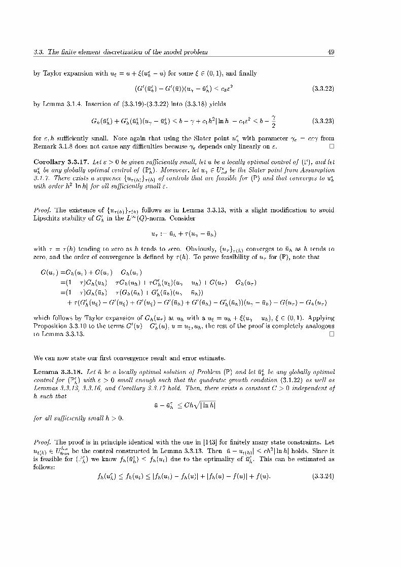
3.3. The �nite element discretization of the model problem 49
by Taylor expansion with u� = �u+ �(�u"h � �u) for some � 2 (0; 1), and �nally
(G0(�u"h)�G0(�u))(u � �u"h) � c3"2 (3.3.22)
by Lemma 3.1.4. Insertion of (3.3.19)-(3.3.22) into (3.3.18) yields
Gh(�u"h) +G0h(�u
"h)(u � �u"h) � b� + c1h
2j lnhj+ c4"2 � b�
2(3.3.23)
for "; h su�ciently small. Note again that using the Slater point u" with parameter " = c" fromRemark 3.1.8 does not cause any di�culties because " depends only linearly on ".
Corollary 3.3.17. Let " > 0 be given su�ciently small, let �u be a locally optimal control of (P), and let�u"h be any globally optimal control of (P"h). Moreover, let u 2 U"ad be the Slater point from Assumption3.1.7. There exists a sequence fu�(h)g�(h) of controls that are feasible for (P) and that converges to �u"hwith order h2j lnhj for all su�ciently small ".
Proof. The existence of fu�(h)g�(h) follows as in Lemma 3.3.13, with a slight modi�cation to avoidLipschitz stability of G0h in the L1(Q)-norm. Consider
u� := �uh + �(u � �uh)
with � = �(h) tending to zero as h tends to zero. Obviously, fu�g�(h) converges to �uh as h tends tozero, and the order of convergence is de�ned by �(h). To prove feasibility of u� for (P), note that
G(u� ) =Gh(u� ) +G(u� )�Gh(u� )
=(1� �)Gh(�uh) + �Gh(�uh) + �G0h(u�)(u � �uh) +G(u� )�Gh(u� )
=(1� �)Gh(�uh) + �(Gh(�uh) +G0h(�uh)(u � �uh))
+ �(G0h(u�)�G0(u�) +G0(u�)�G0(�uh) +G0(�uh)�G0h(�uh))(u � �uh) +G(u� )�Gh(u� )
which follows by Taylor expansion of Gh(u� ) at �uh with a u� = �uh + �(u � �uh), � 2 (0; 1). ApplyingProposition 3.3.10 to the terms G0(u)�G0h(u), u = u�; �uh, the rest of the proof is completely analogousto Lemma 3.3.13.
We can now state our �rst convergence result and error estimate.
Lemma 3.3.18. Let �u be a locally optimal solution of Problem (P) and let �u"h be any globally optimalcontrol for (P"h) with " > 0 small enough such that the quadratic growth condition (3.1.22) as well asLemmas 3.3.13, 3.3.16, and Corollary 3.3.17 hold. Then, there exists a constant C > 0 independent ofh such that
j�u� �u"hj � Chpj lnhj
for all su�ciently small h > 0.
Proof. The proof is in principle identical with the one in [143] for �nitely many state constraints. Let
ut(h) 2 Uh;"feas be the control constructed in Lemma 3.3.13. Then j�u � ut(h)j � ch2j lnhj holds. Since itis feasible for (P"h) we know fh(�u
"h) � fh(ut) due to the optimality of �u"h. This can be estimated as
follows:
fh(�u"h) � fh(ut) � jfh(ut)� fh(�u)j+ jfh(�u)� f(�u)j+ f(�u): (3.3.24)
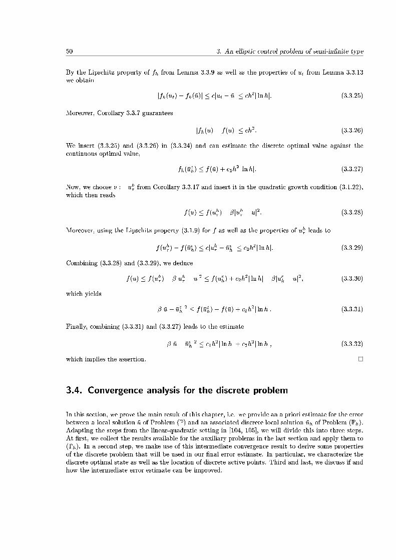
50 3. An elliptic control problem of semi-in�nite type
By the Lipschitz property of fh from Lemma 3.3.9 as well as the properties of ut from Lemma 3.3.13we obtain
jfh(ut)� fh(�u)j � cjut � �uj � ch2j lnhj: (3.3.25)
Moreover, Corollary 3.3.7 guarantees
jfh(�u)� f(�u)j � ch2: (3.3.26)
We insert (3.3.25) and (3.3.26) in (3.3.24) and can estimate the discrete optimal value against thecontinuous optimal value,
fh(�u"h) � f(�u) + c1h
2j lnhj: (3.3.27)
Now, we choose v := uh� from Corollary 3.3.17 and insert it in the quadratic growth condition (3.1.22),which then reads
f(�u) � f(uh� )� �juh� � �uj2: (3.3.28)
Moreover, using the Lipschitz property (3.1.9) for f as well as the properties of uh� leads to
f(uh� )� f(�u"h) � cjuh� � �u"hj � c2h2j lnhj: (3.3.29)
Combining (3.3.28) and (3.3.29), we deduce
f(�u) � f(uh� )� �juh� � �uj2 � f(�u"h) + c2h2j lnhj � �j�u"h � �uj2; (3.3.30)
which yields
�j�u� �u"hj2 � f(�u"h)� f(�u) + c2h2j lnhj: (3.3.31)
Finally, combining (3.3.31) and (3.3.27) leads to the estimate
�j�u� �u"hj2 � c1h2j lnhj+ c2h
2j lnhj; (3.3.32)
which implies the assertion.
3.4. Convergence analysis for the discrete problem
In this section, we prove the main result of this chapter, i.e. we provide an a priori estimate for the errorbetween a local solution �u of Problem (P) and an associated discrete local solution �uh of Problem (Ph).Adapting the steps from the linear-quadratic setting in [104, 105], we will divide this into three steps.At �rst, we collect the results available for the auxiliary problems in the last section and apply them to(Ph). In a second step, we make use of this intermediate convergence result to derive some propertiesof the discrete problem that will be used in our �nal error estimate. In particular, we characterize thediscrete optimal state as well as the location of discrete active points. Third and last, we discuss if andhow the intermediate error estimate can be improved.
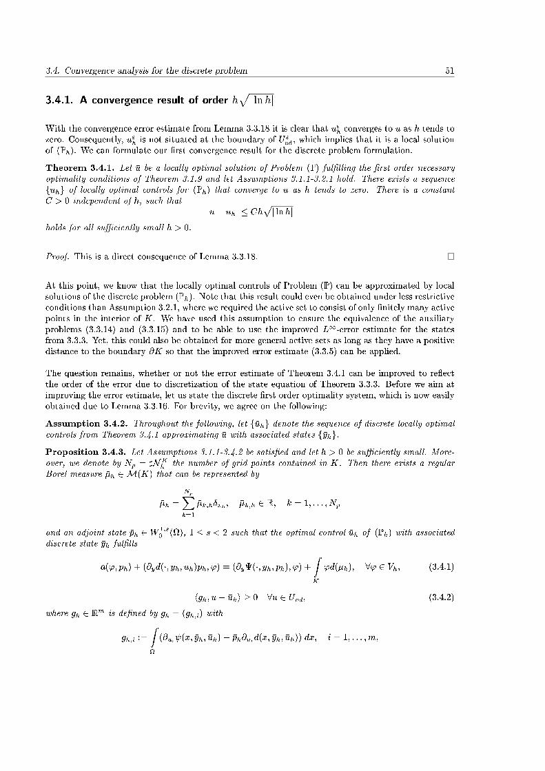
3.4. Convergence analysis for the discrete problem 51
3.4.1. A convergence result of order hpj lnhj
With the convergence error estimate from Lemma 3.3.18 it is clear that �u"h converges to �u as h tends tozero. Consequently, �u"h is not situated at the boundary of U"ad, which implies that it is a local solutionof (Ph). We can formulate our �rst convergence result for the discrete problem formulation.
Theorem 3.4.1. Let �u be a locally optimal solution of Problem (P) ful�lling the �rst order necessaryoptimality conditions of Theorem 3.1.9 and let Assumptions 3.1.1-3.2.1 hold. There exists a sequencef�uhg of locally optimal controls for (Ph) that converge to �u as h tends to zero. There is a constantC > 0 independent of h, such that
j�u� �uhj � Chpj lnhj
holds for all su�ciently small h > 0.
Proof. This is a direct consequence of Lemma 3.3.18.
At this point, we know that the locally optimal controls of Problem (P) can be approximated by localsolutions of the discrete problem (Ph). Note that this result could even be obtained under less restrictiveconditions than Assumption 3.2.1, where we required the active set to consist of only �nitely many activepoints in the interior of K. We have used this assumption to ensure the equivalence of the auxiliaryproblems (3.3.14) and (3.3.15) and to be able to use the improved L1-error estimate for the statesfrom 3.3.3. Yet, this could also be obtained for more general active sets as long as they have a positivedistance to the boundary @K so that the improved error estimate (3.3.5) can be applied.
The question remains, whether or not the error estimate of Theorem 3.4.1 can be improved to re ectthe order of the error due to discretization of the state equation of Theorem 3.3.3. Before we aim atimproving the error estimate, let us state the discrete �rst order optimality system, which is now easilyobtained due to Lemma 3.3.16. For brevity, we agree on the following:
Assumption 3.4.2. Throughout the following, let f�uhg denote the sequence of discrete locally optimalcontrols from Theorem 3.4.1 approximating �u with associated states f�yhg.Proposition 3.4.3. Let Assumptions 3.1.1-3.4.2 be satis�ed and let h > 0 be su�ciently small. More-over, we denote by Np = ]NK
h the number of grid points contained in K. Then there exists a regularBorel measure ��h 2M(K) that can be represented by
��h =
NpXk=1
��k;h�xk ; ��k;h 2 R; k = 1; : : : ; Np
and an adjoint state �ph 2 W 1;s0 (), 1 � s < 2 such that the optimal control �uh of (Ph) with associated
discrete state �yh ful�lls
a('; �ph) + (@yd(�; �yh; �uh)ph; ') = (@y(�; �yh; �ph); ') +ZK
'd(��h); 8' 2 Vh; (3.4.1)
hgh; u� �uhi � 0 8u 2 Uad; (3.4.2)
where gh 2 Rm is de�ned by gh = (gh;i) with
gh;i :=
Z
(@ui (x; �yh; �uh)� �ph@uid(x; �yh; �uh)) dx; i = 1; : : : ;m;

52 3. An elliptic control problem of semi-in�nite type
as well as the complementary slackness conditionZK
(�yh � b) d��h = 0; ��h � 0: (3.4.3)
Proof. This follows as in [18] or [2], where semilinear problems with Robin or Neumann-type boundaryconditions have been considered. A linear-quadratic problem with Dirichlet boundary conditions andcontrol functions has been taken into account in [17].
Remark 3.4.4. In all what follows, we identify ��h with the associated Np-vector of real numbers ��k;h,k = 1; : : : ; Np.
Again, a formulation with Lagrange multipliers associated with the control constraints is easily obtained.If the tuple (�uh; �yh; �ph; ��h) 2 Uad�Vh�W 1;s()�M(K) ful�lls the setting of Proposition 3.4.3, thereexist nonnegative Lagrange multipliers ��ah; ��
bh 2 Rm such that the variational inequality (3.4.2) can
equivalently be writtengh;i + ��bh;i � ��ah;i = 0 (3.4.4)
andhua � �uh; ��
ahi = h�uh � ub; ��
bhi = 0; (3.4.5)
cf. again [144]. Alternatively, the �rst order necessary optimality conditions of Proposition 3.4.3 canbe expressed with the help of the discrete Lagrangian
Lh : U �M(K)! R; Lh(u; �h) := fh(u) +
ZZK
(Gh(u)� b) d�h(x):
As an equivalent to Proposition 3.4.3 we then obtain
L0h(�uh; ��h)(u� �uh) � 0 8u 2 Uad; (3.4.6)
orL0h(�uh; ��h) + ��bh � ��ah = 0; (3.4.7)
combined with the complementary slackness condition (3.4.3), and (3.4.5), respectively, for the nonneg-ative Lagrange multipliers ��h; ��
ah; ��
bh, as in the continuous setting.
3.4.2. Some properties of the discrete problem
In this section, we will provide all technical results that are necessary to improve the intermediate errorestimate. The steps from the linear-quadratic setting in e.g. [105] need only minor modi�cations dueto the nonlinear control-to-state whereever a derivative of the control-to-state operator is used. Theoverall goal of this section is to provide an estimate for the distance of discrete and continuous activepoints. This will be a key argument in the later proof of convergence, and it is also the main di�erenceto the completely �nite dimensional problem in [106], where the constraints were considered in �xedpoints. Eventually, we will make use of the fact that the active points on the discrete and the continuouslevel have a similar distance as the discrete and continuous controls. This will be useful in Taylor-typearguments. In Section 3.2.2, we have already discussed some structural properties of the continuousoptimal state �y. With the convergence result of Theorem 3.4.1 let us now discuss the structure of thediscrete state.
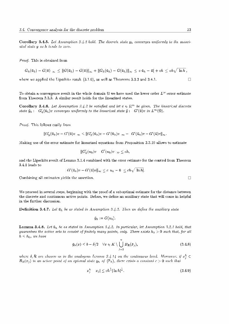
3.4. Convergence analysis for the discrete problem 53
Corollary 3.4.5. Let Assumption 3.4.2 hold. The discrete state �yh converges uniformly to the associ-ated state �y as h tends to zero.
Proof. This is obtained from
kGh(�uh) � G(�u)k1 � kG(�uh) � G(�u)k1 + kGh(�uh) � G(�uh)k1 � cj�uh � �uj + ch � chpj lnhj;
where we applied the Lipschitz result (3.1.6), as well as Theorems 3.3.3 and 3.4.1.
To obtain a convergence result in the whole domain we have used the lower order L1-error estimatefrom Theorem 3.3.3. A similar result holds for the linearized states.
Corollary 3.4.6. Let Assumption 3.4.2 be satis�ed and let v 2 Rm be given. The linearized discretestate ~yh := G0h(�uh)v converges uniformly to the linearized state ~y := G0(�u)v in L1().
Proof. This follows easily from
kG0h(�uh)v �G0(�u)vk1 � kG0h(�uh)v �G0(�uh)vk1 + kG0(�uh)v �G0(�u)vk1:
Making use of the error estimate for linearized equations from Proposition 3.3.10 allows to estimate
kG0h(�uh)v �G0(�uh)vk1 � ch;
and the Lipschitz result of Lemma 3.1.4 combined with the error estimate for the control from Theorem3.4.1 leads to
kG0(�uh)v �G0(�u)vk1 � c juh � �uj � chpj lnhj;
Combining all estimates yields the assertion.
We proceed in several steps, beginning with the proof of a suboptimal estimate for the distance betweenthe discrete and continuous active points. Before, we de�ne an auxiliary state that will come in helpfulin the further discussion.
De�nition 3.4.7. Let �uh be as stated in Assumption 3.4.2. Then we de�ne the auxiliary state
~yh := G(�uh):
Lemma 3.4.8. Let �uh be as stated in Assumption 3.4.2. In particular, let Assumption 3.2.1 hold, thatguarantees the active sets to consist of �nitely many points, only. There exists h0 > 0 such that, for allh � h0, we have
�yh(x) � b� �=2 8x 2 K nn[j=1
BR(�xj); (3.4.8)
where �;R are chosen as in the analogous Lemma 3.4.14 on the continuous level. Moreover, if �xhj 2BR(�xj) is an active point of an optimal state �yh of (Ph), there exists a constant c > 0 such that
j�xhj � �xj j � ch12 j lnhj 14 : (3.4.9)

54 3. An elliptic control problem of semi-in�nite type
Proof. Inequality (3.4.8) is a direct consequence of the uniform convergence stated in Corollary 3.4.5and Assumption 3.2.1 on the structure of the active set. This implies in particular that the discretestate can only be active in a neighborhood of the continuous active points �xj , j = 1; : : : ; n, with �niteradius R. Assume therefore �xhj 2 BR(�xj) to be an active point of (Ph), i.e. �yh(�x
hj ) = b. We observe
�yh(�xhj ) = �y(�xhj ) + (~yh � �y)(�xhj ) + (�yh � ~yh)(�x
hj ); (3.4.10)
where ~yh is de�ned in De�nition 3.4.7. Then, by the Lipschitz stability result (3.1.6) for the continuouscontrol-to-state operator G and the error estimate of Theorem 3.4.1, we obtain
k~yh � �yk1 = kG(�uh)�G(�u)k1 � cj�uh � �uj � chpj lnhj: (3.4.11)
In addition, Theorem 3.3.3 guarantees
k�yh � ~yhk1;K = kGh(�uh)�G(�uh)k1;K � ch2j lnhj (3.4.12)
in K. Inserting both estimates into (3.4.10) delivers
�yh(�xhj ) � �y(�xhj ) + ch
pj lnhj+ ch2j lnhj: (3.4.13)
Finally, applying (3.2.2) to estimate �y(�xhj ) in (3.4.13) leads to
�yh(�xhj ) � b� !
4j�xhj � �xj j2 + ch
pj lnhj; (3.4.14)
and with �yh(�xhj ) = b, this can be transformed to
j�xj � �xhj j � ch12 j lnhj 14 ;
and the assertion is obtained.
In the following, our main goal is to improve this suboptimal estimate. This involves distance estimateson two levels. First, we compare active points of �y (or maxima of �y) with maxima of ~yh. Noting that�y = G(�u) and ~yh = G(�uh) makes clear that we only take into account the in uence of the controls. Ina second step, we will estimate the distance between active points of ~yh and �yh, which estimates thein uence of the discretization of the state equation.
Lemma 3.4.9. For each active point �xj, j = 1; : : : ; n, of �y = G(�u), there exists a unique local maximum~xhj 2 BR(�xj) of ~yh = G(�uh). Moreover, the estimate
j�xj � ~xhj j � Chpj lnhj
is satis�ed for a constant C > 0 independent of h.
Proof. For a control u 2 U we denote by y = G(u) the associated state on the continuous level, andde�ne the function
F (x; u) := ry(x):Notice that F (x; u) = 0 describes a necessary condition for a local maximum of y at x. Hence, weobserve that F (�xj ; �u) = 0 holds for all j = 1; : : : ; n, since due to Assumption 3.2.1, �y admits a localmaximum in �xj for all j = 1; : : : ; n. Notice further that by the same assumption the matrix
@F
@x(�xj ; �u) = r2�y(�xj)
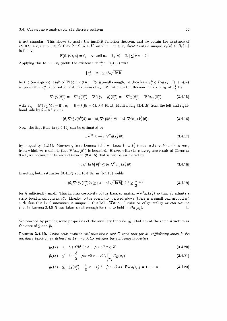
3.4. Convergence analysis for the discrete problem 55
is not singular. This allows to apply the implicit function theorem, and we obtain the existence ofconstants r; �; c > 0 such that for all u 2 U with ju � �uj � � , there exists a unique ~xj(u) 2 Br(�xj)ful�lling
F (~xj(u); u) = 0; as well as j~xj(u)� �xj j � cju� �uj:Applying this to u := �uh yields the existence of ~xhj := ~xj(�uh) with
j~xhj � �xj j � chpj lnhj
by the convergence result of Theorem 3.4.1. For h small enough, we then have ~xhj 2 BR(�xj). It remainsto prove that ~xhj is indeed a local maximum of ~yh. We estimate the Hessian matrix of ~yh at ~xhj by
�r2~yh(~xhj ) = �r2�y(~xhj )�r2(~yh � �y)(~xhj ) = �r2�y(~xhj )�r2zu�(~x
hj ) (3.4.15)
with zu� = G0(u�)(�uh � �u), u� = �u+ �(�uh � �u), � 2 (0; 1). Multiplying (3.4.15) from the left and right-hand side by � 2 R2 yields
�h�;r2~yh(~xhj )�i = �h�;r2�y(~xhj )�i � h�;r2zu�(~x
hj )�i: (3.4.16)
Now, the �rst item in (3.4.16) can be estimated by
!j�j2 � �h�;r2�y(~xhj )�i (3.4.17)
by inequality (3.2.1). Moreover, from Lemma 3.4.9 we know that ~xhj tends to �xj as h tends to zero,
from which we conclude that r2zu�(~xhj ) is bounded. Hence, with the convergence result of Theorem
3.4.1, we obtain for the second term in (3.4.16) that it can be estimated by
�chpj lnhjj�j2 � h�;r2zu�(~x
hj )�i: (3.4.18)
Inserting both estimates (3.4.17) and (3.4.18) in (3.4.16) yields
�h�;r2~yh(~xhj )�i � (! � ch
pj lnhj)j�j2 � !
2j�j2 (3.4.19)
for h su�ciently small. This implies coercivity of the Hessian matrix �r2~yh(~xhj ) so that ~yh admits a
strict local maximum in ~xhj . Thanks to the coercivity derived above, there is a small ball around ~xhjsuch that this local maximum is unique in this ball. Without limitation of generality we can assumethat in Lemma 3.4.8 R was taken small enough for this to hold in BR(�xj).
We proceed by proving some properties of the auxiliary function ~yh, that are of the same structure asthe ones of �y and �yh.
Lemma 3.4.10. There exist positive real numbers r and C such that for all su�ciently small h theauxiliary function ~yh de�ned in Lemma 3.4.9 satis�es the following properties:
~yh(x) � b+ Ch2j lnhj for all x 2 K (3.4.20)
~yh(x) � b� �
2for all x 2 K n
n[j=1
BR(�xj) (3.4.21)
~yh(x) � ~yh(~xhj )�
!
8jx� ~xhj j2 for all x 2 Br(�xj); j = 1; : : : ; n: (3.4.22)
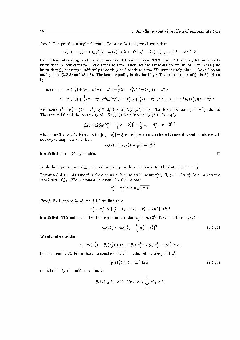
56 3. An elliptic control problem of semi-in�nite type
Proof. The proof is straight-forward. To prove (3.4.20), we observe that
~yh(x) = �yh(x) + (~yh(x)� �yh(x)) � b+ kG(�uh)�Gh(�uh)k1;K � b+ ch2j lnhjby the feasibility of �yh and the accuracy result from Theorem 3.3.3. From Theorem 3.4.1 we alreadyknow that �uh converges to �u as h tends to zero. Then, by the Lipschitz continuity of G in L1() weknow that ~yh converges uniformly towards �y as h tends to zero. We immediately obtain (3.4.21) as ananalogue to (3.2.3) and (3.4.8). The last inequality is obtained by a Taylor expansion of ~yh in ~xhj , givenby
~yh(x) = ~yh(~xhj ) +r~yh(~x
hj )(x� ~xhj ) +
1
2hx� ~xhj ;r2~yh(x
�j)(x� ~xhj )i
� ~yh(~xhj ) +
1
2hx� ~xhj ;r2~yh(~x
hj )(x� ~xhj )i+
1
2hx� ~xhj ; (r2~yh(x�)�r2~yh(~x
hj ))(x� ~xhj )i
with some x�j = ~xhj + �(x � ~xhj ), � 2 (0; 1), since r~yh(~xhj ) = 0. The H�older continuity of r2~yh due to
Theorem 2.4.6 and the coercivity of �r2~y(~xhj ) from inequality (3.4.19) imply
~yh(x) � ~yh(~xhj )�
!
4jx� ~xhj j2 +
c
2jx� � ~xhj j� jx� ~xhj j2
with some 0 < � < 1. Hence, with jx� � ~xhj j = �jx� ~xhj j, we obtain the existence of a real number r > 0not depending on h such that
~yh(x) � ~yh(~xhj )�
!
8jx� ~xhj j2
is satis�ed if jx� ~xhj j � r holds.
With these properties of ~yh at hand, we can provide an estimate for the distance j~xhj � �xhj j.Lemma 3.4.11. Assume that there exists a discrete active point �xhj 2 BR(�xj). Let ~xhj be an associatedmaximum of ~yh. There exists a constant C > 0 such that
j�xhj � ~xhj j � Chpj lnhj:
Proof. By Lemmas 3.4.8 and 3.4.9 we �nd that
j�xhj � ~xhj j � j�xhj � �xj j+ j�xj � ~xhj j � ch12 j lnhj 14
is satis�ed. This suboptimal estimate guarantees that �xhj 2 Br(~xhj ) for h small enough, i.e.
~yh(�xhj ) � ~yh(~x
hj )�
!
8j�xhj � ~xhj j2: (3.4.23)
We also observe that
b = �yh(�xhj ) = ~yh(�x
hj ) + (�yh � ~yh)(�x
hj ) � ~yh(�x
hj ) + ch2j lnhj
by Theorem 3.3.3. From that, we conclude that for a discrete active point �xhj
~yh(�xhj ) � b� ch2j lnhj (3.4.24)
must hold. By the uniform estimate
~yh(x) � b� �=2 8x 2 K nn[j=1
BR(�xj);

3.4. Convergence analysis for the discrete problem 57
stated in Lemma 3.4.10, this can only be true inside the balls BR(�xj). Hence, combining (3.4.23) and(3.4.24) gives a necessary condition for activity of the discrete state �yh at �xhj , which reads
b� ch2j lnhj � ~yh(�xhj ) � ~yh(~x
hj )�
!
8j�xhj � ~xhj j2:
This can be transferred into
j�xhj � ~xhj j2 � ch2j lnhj+ 8
!(~yh(~x
hj )� b) � ch2j lnhj+ 8
!
��yh(~x
hj )� b+ (~yh � �yh)(~x
hj )� � ch2j lnhj
where the last inequality follows from �yh(~xhj ) � b and Theorem 3.3.3.
We now directly obtain an improved estimate for the distance j�xj � �xhj j:
Corollary 3.4.12. For any discrete active point �xhj 2 BR(�xj) we obtain the distance estimate
j�xj � �xhj j � Chplnh
for some C > 0.
Proof. By Lemmas 3.4.9 and 3.4.10 this follows from j�xj � �xhj j � j�xj � ~xhj j+ j~xhj � �xhj j:
Note that neither the existence of a discrete active point �xhj in the neighborhood of �xj , nor its uniquenessis guaranteed at this time. The strong activity property will provide existence of active points of �yh inthe neighborhoods of all strongly active points �xj , j 2 A�y, for all su�ciently small h. To prepare thisstatement, we proceed with an intermediate result.
Lemma 3.4.13. Let fhngn2N be a sequence of positive real numbers converging to zero as n tends toin�nity, and let f�uhg be the sequence of locally optimal solutions of (Ph) from Assumption 3.4.2. Anysequence f��hngn2N of Lagrange multipliers for (Ph) is bounded in M(K).
Proof. This is a standard conclusion from the Slater condition. The proof is given for convenience. Wehave already pointed out in Lemma 3.3.16 that the Slater point u is also a Slater point for the optimalcontrol of Problem (P"h) and by the intermediate convergence result also for (Ph). For simplicity, we omitthe subscript n in hn and the associated optimal controls, states, and Lagrange multipliers. Insertingu 2 Uad into the variational inequality (3.4.6) for �uh and making use of the complementary slacknesscondition (3.4.3) and the Slater point property of Lemma 3.3.16, we �nd
0 � L0h(�uh; ��h)(u � �uh)
= f 0h(�uh)(u � �uh) +
ZK
G0h(�uh)(u � �uh)d��h(x)
= f 0h(�uh)(u � �uh) +
ZK
(Gh(�uh) +G0h(�uh)(u � �uh)� b)d��h(x) +
ZK
(b�Gh(�uh))d��h(x)
= f 0h(�uh)(u � �uh) +
ZK
(Gh(�uh) +G0h(�uh)(u � �uh)� b)d��h(x)
� f 0h(�uh)(u � �uh)�
2
ZK
1 � d��h(x)

58 3. An elliptic control problem of semi-in�nite type
for all h su�ciently small, which yields
2
ZK
1 � d��h(x) � f 0h(�uh)(u � �uh):
Moreover, the sequence f�uhg is bounded as h tends to zero. This follows directly from the boundednessof Uad. Therefore, we obtain
k��hkM(K) =
ZK
d��h(x) � c
:
Lemma 3.4.14. Let Assumptions 3.1.1-3.4.2 hold. For any j 2 A�y, there exists a constant C > 0 andat least one point �xhj 2 BR(�xj) of Problem (Ph) where �yh is active, i.e. �yh(�x
hj ) = b, with
j�xj � �xhj j � Chpj lnhj: (3.4.25)
Proof. Let fhng > 0 be a sequence of mesh sizes converging to zero, and denote by f�ung, f�yng, andf��ng the sequences of discrete optimal control, state, and an associated Lagrange multiplier associatedwith hn in a neighborhood of �u, cf. Assumption 3.4.2. Now let us assume the contrary: then, thereexists an index j 2 A�y and for all n a positive hn < 1
n such that �yn(x) := �yhn(x) < b holds for allx 2 K \BR(�xj). Consequently, we can assume
�yn(x) < b 8 x 2 BR(�xj);
and by the complementary slackness condition (3.4.3), we have
��njBR(�xj)= 0 (3.4.26)
for all n. By Lemma 3.4.13, the sequence f��ng is bounded in M(K). Therefore, we can select asubsequence converging weakly� to some � 2M(K). Let, w.l.o.g., f��ng be this sub-sequence. Moreover,we already know that �un ! �u in Rm and
G0h(�un)(u� �un)! G0(�u)(u� �u)
in C(K) by Corollary 3.4.6. We now verify that � is a Lagrange multiplier associated with �y: we have
f 0hn(�un)(u� �un) +
ZK
G0h(�un)(u� �un)d��n(x) � 0 (3.4.27)
for all u 2 Uad and all n 2 N. Notice that all sequences except f��hg converge strongly. Passing to thelimit in (3.4.27) yields
f 0(�u)(u� �u) +
ZK
G0(�u)(u� �u)d�(x) � 0;
i.e. � satis�es the variational inequality (3.1.19). Moreover, we obviously have � � 0. Finally, passingto the limit in Z
K
(�yn � b)d��n(x) = 0;
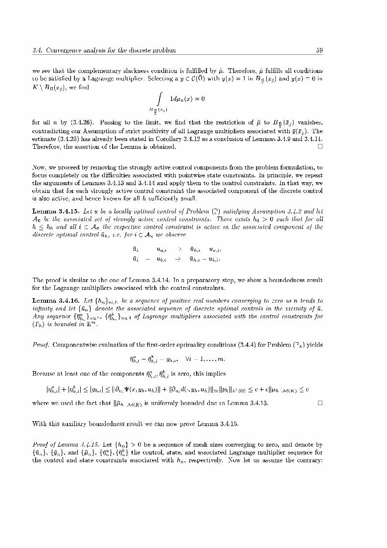
3.4. Convergence analysis for the discrete problem 59
we see that the complementary slackness condition is ful�lled by �. Therefore, � ful�lls all conditionsto be satis�ed by a Lagrange multiplier. Selecting a y 2 C(�) with y(x) = 1 in BR
2(�xj) and y(x) � 0 in
K nBR(�xj), we �nd ZBR
2(�xj)
1d��n(x) = 0
for all n by (3.4.26). Passing to the limit, we �nd that the restriction of � to BR2(�xj) vanishes,
contradicting our Assumption of strict positivity of all Lagrange multipliers associated with �y(�xj). Theestimate (3.4.25) has already been stated in Corollary 3.4.12 as a conclusion of Lemmas 3.4.9 and 3.4.11.Therefore, the assertion of the Lemma is obtained.
Now, we proceed by removing the strongly active control components from the problem formulation, tofocus completely on the di�culties associated with pointwise state constraints. In principle, we repeatthe arguments of Lemmas 3.4.13 and 3.4.14 and apply them to the control constraints. In that way, weobtain that for each strongly active control constraint the associated component of the discrete controlis also active, and hence known for all h su�ciently small.
Lemma 3.4.15. Let �u be a locally optimal control of Problem (P) satisfying Assumption 3.4.2 and letA�u be the associated set of strongly active control constraints. There exists h0 > 0 such that for allh � h0 and all i 2 A�u the respective control constraint is active in the associated component of thediscrete optimal control �uh, i.e. for i 2 A�u we observe
�ui = ua;i ) �uh;i = ua;i;
�ui = ub;i ) �uh;i = ub;i:
The proof is similar to the one of Lemma 3.4.14. In a preparatory step, we show a boundedness resultfor the Lagrange multipliers associated with the control constraints.
Lemma 3.4.16. Let fhngn2N be a sequence of positive real numbers converging to zero as n tends toin�nity and let f�ung denote the associated sequence of discrete optimal controls in the vicinity of �u.Any sequence f��ahngn2N, f��bhngn2N of Lagrange multipliers associated with the control constraints for(Ph) is bounded in Rm.
Proof. Componentwise evaluation of the �rst-order optimality conditions (3.4.4) for Problem (Ph) yields
��ah;i � ��bh;i = gh;i; 8i = 1; : : : ;m:
Because at least one of the components ��ah;i; ��bh;i is zero, this implies
j��ah;ij+ j��bh;ij � jgh;ij � k@ui(x; �yh; �uh)k+ k@uid(�; �yh; �uh)k1k�phkL1() � c+ ck��hkM(K) � c
where we used the fact that k��hkM(K) is uniformly bounded due to Lemma 3.4.13.
With this auxiliary boundedness result we can now prove Lemma 3.4.15.
Proof of Lemma 3.4.15. Let fhng > 0 be a sequence of mesh sizes converging to zero, and denote byf�ung, f�yng, and f��ng, f��ang; f��bng the control, state, and associated Lagrange multiplier sequence forthe control and state constraints associated with hn, respectively. Now let us assume the contrary:
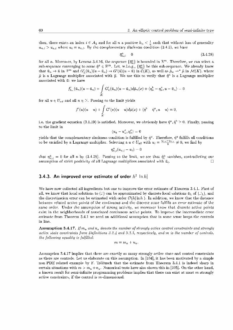
60 3. An elliptic control problem of semi-in�nite type
then, there exists an index i 2 A�u and for all n a positive hn <1n such that without loss of generality
�un;i > ua;i where �ui = ua;i. By the complementary slackness condition (3.4.5), we have
��an;i = 0 (3.4.28)
for all n. Moreover, by Lemma 3.4.16, the sequence f��ang is bounded in Rm. Therefore, we can select asub-sequence converging to some �a 2 Rm. Let, w.l.o.g., f��ang be this sub-sequence. We already knowthat �un ! �u in Rm and G0h(�un)(u� �un)! G0(�u)(u� �u) in C(K), as well as ��n *
� � in M(K), where� is a Lagrange multiplier associated with �y. We use this to verify that �a is a Lagrange multiplierassociated with �u: we have
f 0hn(�un)(u� �un) +
ZK
G0h(�un)(u� �un)d��n(x) + h�bn � �an; u� �uni = 0
for all u 2 Uad and all n 2 N. Passing to the limit yields
f 0(�u)(u� �u) +
ZK
G0(�u)(u� �u)d�(x) + h�b � �a; u� �ui = 0;
i.e. the gradient equation (3.1.19) is satis�ed. Moreover, we obviously have �a; �b � 0. Finally, passingto the limit in
hua � �uan; �ani = 0
yields that the complementary slackness condition is ful�lled by �a. Therefore, �a ful�lls all conditionsto be satis�ed by a Lagrange multiplier. Selecting a u 2 Uad with ui =
ub;i�ua;i2 6= 0, we �nd by
�an;i(ua;i � ui) = 0
that �an;i = 0 for all n by (3.4.28). Passing to the limit, we see that �ai vanishes, contradicting ourassumption of strict positivity of all Lagrange multipliers associated with �ui.
3.4.3. An improved error estimate of order h2j lnhj
We have now collected all ingredients but one to improve the error estimate of Theorem 3.4.1. First ofall, we know that local solutions to (P) can be approximated by discrete local solutions �uh of (Ph), andthe discretization error can be estimated with order O(hj lnhj). In addition, we know that the distancebetween related active points of the continuous and the discrete state ful�lls an error estimate of thesame order. Under the assumption of strong activity, we moreover know that discrete active pointsexist in the neighborhoods of associated continuous active points. To improve the intermediate errorestimate from Theorem 3.4.1 we need an additional assumption that in some sense keeps the controlsin line.
Assumption 3.4.17. If ma and na denote the number of strongly active control constraints and stronglyactive state constraints from De�nitions 3.2.4 and 3.2.5, respectively, and m is the number of controls,the following equality is ful�lled:
m = ma + na:
Assumption 3.4.17 implies that there are exactly as many strongly active state and control constraintsas there are controls. Let us elaborate on this assumption. In [104], it has been motivated by a simplenon-PDE-related example by F. Tr�oltzsch that the estimate from Theorem 3.4.1 is indeed sharp incertain situations with m > ma+na. Numerical tests have also shown this in [105]. On the other hand,a known result for semi-in�nite programming problems implies that there can exist at most m stronglyactive constraints, if the control is m-dimensional.
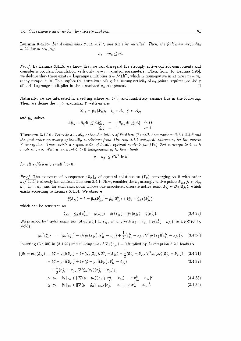
3.4. Convergence analysis for the discrete problem 61
Lemma 3.4.18. Let Assumptions 3.1.1, 3.1.7, and 3.2.1 be satis�ed. Then, the following inequalityholds for m;ma; na:
na +ma � m:
Proof. By Lemma 3.4.15, we know that we can disregard the strongly active control components andconsider a problem formulation with only m �ma control parameters. Then, from [16, Lemma 4.98],we deduce that there exists a Lagrange multiplier � 2M(K), which is nonnegative in at most m�ma
many components. This implies the assertion noting that strong activity of na points requires positivityof each Lagrange multiplier in the associated na components.
Naturally, we are interested in a setting where na > 0, and implicitely assume this in the following.Then, we de�ne the na � na-matrix Y with entries
Yl;k = ~yik(�xjl); ik 2 A�u; jl 2 A�y;
and ~yik solvesA~yik + @yd(�; �y; �u)~yik = �@uik d(�; �y; �u) in
~yik = 0 on �:
Theorem 3.4.19. Let �u be a locally optimal solution of Problem (P) with Assumptions 3.1.1-3.4.2 andthe �rst-order necessary optimality conditions from Theorem 3.1.9 satis�ed. Moreover, let the matrixY be regular. There exists a sequence �uh of locally optimal controls for (Ph) that converge to �u as htends to zero. With a constant C > 0 independent of h, there holds
j�u� �uhj � Ch2j lnhjfor all su�ciently small h > 0.
Proof. The existence of a sequence f�uhgh of optimal solutions to (Ph) converging to �u with orderhpj lnhj is already known from Theorem 3.4.1. Now, consider the na strongly active points �xjk , jk 2 A�y,k = 1; : : : na, and for each such point choose one associated discrete active point �xhjk 2 BR(�xjk), whichexists according to Lemma 3.4.14. We observe
�y(�xjk) = b = �yh(�xhjk) = ~yh(�x
hjk) + (�yh � ~yh) (�x
hjk);
which can be rewritten as
(�yh � ~yh)(�xhjk) = �y(�xjk)� ~yh(�xjk) + ~yh(�xjk)� ~y(�xhjk): (3.4.29)
We proceed by Taylor expansion of ~yh(�xhjk) at �xjk , which, with x� = �xjk + �(�xhjk � �xjk) for a � 2 (0; 1),
yields
~yh(�xhjk) = ~yh(�xjk) + hr~yh(�xjk); �x
hjk � �xjki+
1
2h�xhjk � �xjk ;r2~yh(x�)(�x
hjk � �xjk)i: (3.4.30)
Inserting (3.4.30) in (3.4.29) and making use of r�y(�xjk) = 0 implied by Assumption 3.2.1 leads to
j(�yh � ~yh)(�xjk)j =j(�y � ~yh)(�xjk)� hr(~yh(�xjk); �xhjk � �xjki �1
2h�xhjk � �xjk ;r2~yh(x�)(�x
hjk � �xjk)ij (3.4.31)
=j(�y � ~yh)(�xjk) + hr(�y � ~yh)(�xjk); �xhjk � �xjki (3.4.32)
� 1
2h�xhjk � �xjk ;r2~yh(x�)(�x
hjk � �xjk)ij
�k�yh � ~yhk1 + jhr(�y � ~yh)(�xjk); �xhjk � �xjkij+ cj�xhjk � �xjk j2 (3.4.33)
�k�yh � ~yhk1 + kr(�y � ~yh)k1;K j�xhjk � �xjk j+ cj�xhjk � �xjk j2: (3.4.34)
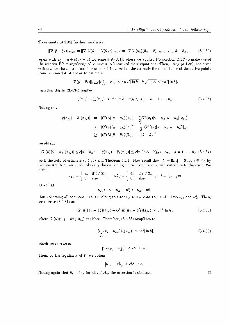
62 3. An elliptic control problem of semi-in�nite type
To estimate (3.4.34) further, we derive
kr(�y � ~yh)k1;K = kr(G(�u)�G(�uh))k1;K = krG0(u�)(�uh � �u)k1;K � c3j�u� �uhj; (3.4.35)
again with u� = �u + �(�uh � �u) for some � 2 (0; 1), where we applied Proposition 2.4.2 to make use ofthe interior W 2;1-regularity of solutions to linearized state equations. Then, using (3.4.35), the errorestimate for the control from Theorem 3.4.1, as well as the estimate for the distance of the active pointsfrom Lemma 3.4.14 allows to estimate
kr(�y � ~yh)k1;K j�xhjk � �xjk j � c hpj lnhj � h
pj lnhj � c h2j lnhj:
Inserting this in (3.4.34) implies
j�y(�xjk)� ~yh(�xjk)j � ch2j lnhj 8jk 2 A�y; k = 1; : : : ; na: (3.4.36)
Noting that
j�y(�xjk)� ~yh(�xjk)j = jG0(�u)(�u� �uh)(�xjk) +1
2G00(u�)[�u� �uh; �u� �uh](�xjk)j
� jG0(�u)(�u� �uh)(�xjk)j �1
2kG00(u�)[�u� �uh; �u� �uh]k1
� jG0(�u)(�u� �uh)(�xjk)j � cj�u� �uhj2
we obtain
jG0(�u)(�u� �uh)(�xjk)j � cj�u� �uhj2 + j�y(�xjk)� ~yh(�xjk)j � ch2j lnhj 8jk 2 A�y; k = 1; : : : ; na (3.4.37)
with the help of estimate (3.4.36) and Theorem 3.4.1. Now recall that j�ui � �uh;ij = 0 for i 2 A�u byLemma 3.4.15. Then, obviously only the remaining control components can contribute to the error. Wede�ne
�uI;i =
��ui if i 2 I�u0 else
; �uhI;i =
��uhi if i 2 I�u0 else
; i = 1; : : : ;m
as well as�uA := �u� �uI ; �uhA := �uh � �uhI ;
thus collecting all components that belong to strongly active constraints of �u into �uA and �uhA. Then,we rewrite (3.4.37) as ��G0(�u)(�uI � �uhI)(�xjk) +G0(�u)(�uA � �uhA)(�xjk)
�� � ch2j lnhj; (3.4.38)
where G0(�u)(�uA � �uhA)(�xjk) vanishes. Therefore, (3.4.38) simpli�es to�����Xi2I�u
(�ui � �uh;i)~yi(�xjk)
����� � ch2j lnhj; (3.4.39)
which we rewrite asjY (�uI�u � �uhI�u)j � ch2j lnhj:
Then, by the regularity of Y , we obtain���uI�u � �uhI�u�� � ch2j lnhj:
Noting again that �ui = �uh;i for all i 2 A�u, the assertion is obtained.
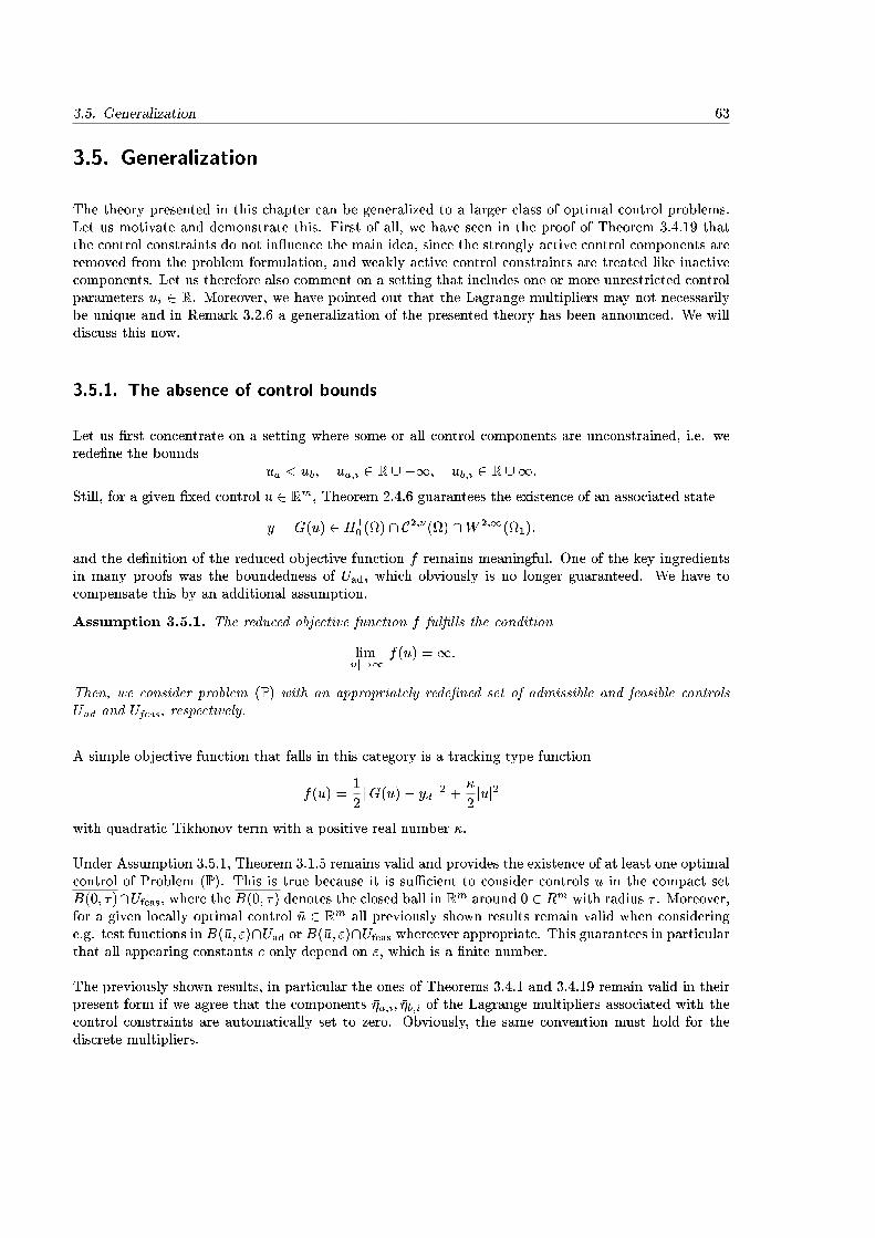
3.5. Generalization 63
3.5. Generalization
The theory presented in this chapter can be generalized to a larger class of optimal control problems.Let us motivate and demonstrate this. First of all, we have seen in the proof of Theorem 3.4.19 thatthe control constraints do not in uence the main idea, since the strongly active control components areremoved from the problem formulation, and weakly active control constraints are treated like inactivecomponents. Let us therefore also comment on a setting that includes one or more unrestricted controlparameters ui 2 R. Moreover, we have pointed out that the Lagrange multipliers may not necessarilybe unique and in Remark 3.2.6 a generalization of the presented theory has been announced. We willdiscuss this now.
3.5.1. The absence of control bounds
Let us �rst concentrate on a setting where some or all control components are unconstrained, i.e. werede�ne the bounds
ua < ub; ua;i 2 R [ �1; ub;i 2 R [1:
Still, for a given �xed control u 2 Rm, Theorem 2.4.6 guarantees the existence of an associated state
y = G(u) 2 H10 () \ C2;�() \W 2;1(1):
and the de�nition of the reduced objective function f remains meaningful. One of the key ingredientsin many proofs was the boundedness of Uad, which obviously is no longer guaranteed. We have tocompensate this by an additional assumption.
Assumption 3.5.1. The reduced objective function f ful�lls the condition
limjuj!1
f(u) =1:
Then, we consider problem (P) with an appropriately rede�ned set of admissible and feasible controlsUad and Ufeas, respectively.
A simple objective function that falls in this category is a tracking type function
f(u) =1
2kG(u)� ydk2 + �
2juj2
with quadratic Tikhonov term with a positive real number �.
Under Assumption 3.5.1, Theorem 3.1.5 remains valid and provides the existence of at least one optimalcontrol of Problem (P). This is true because it is su�cient to consider controls u in the compact setB(0; �)\Ufeas, where the B(0; �) denotes the closed ball in R
m around 0 2 Rm with radius � . Moreover,for a given locally optimal control �u 2 Rm all previously shown results remain valid when consideringe.g. test functions in B(�u; ")\Uad or B(�u; ")\Ufeas whereever appropriate. This guarantees in particularthat all appearing constants c only depend on ", which is a �nite number.
The previously shown results, in particular the ones of Theorems 3.4.1 and 3.4.19 remain valid in theirpresent form if we agree that the components ��a;i; ��b;i of the Lagrange multipliers associated with thecontrol constraints are automatically set to zero. Obviously, the same convention must hold for thediscrete multipliers.
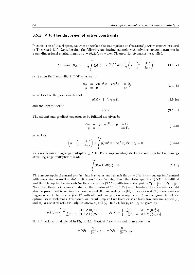
64 3. An elliptic control problem of semi-in�nite type
3.5.2. A further discussion of active constraints
In conclusion of this chapter, we want to weaken the assumptions on the strongly active constraints usedin Theorem 3.4.19. Consider �rst the following motivating example with only one control parameter ina one-dimensional spatial domain := (0; 2�), to which Theorem 3.4.19 cannot be applied.
Minimize J(y; u) :=1
2
2�Z0
�y(x)� sin2 x
�2dx+
1
2
�u�
�2� 4
3�
��2
(3.5.1a)
subject to the linear elliptic PDE constraint
��y = u(sin2 x� cos2 x) in ;y = 0 on �;
(3.5.1b)
as well as the the pointwise bound
y(x) � 1 8 x 2 ; (3.5.1c)
and the control bound
u � 2: (3.5.1d)
The adjoint and gradient equation to be ful�lled are given by
���p = �y � sin2 x+ �� in ;�p = 0 on �;
(3.5.2)
as well as ��u�
�2� 4
3�
��+
2�Z0
�p(sin2 x� cos2 x) dx� ��a = 0; (3.5.3)
for a nonnegative Lagrange multiplier ��a 2 R. The complementary slackness condition for the nonneg-ative Lagrange multiplier �� reads
2�Z0
(�y � 1) d��(x) = 0: (3.5.4)
This convex optimal control problem has been constructed such that �u = 2 is the unique optimal controlwith associated state �y = sin2 x. It is easily veri�ed that then the state equation (3.5.1b) is ful�lledand that the optimal state satis�es the constraints (3.5.1c) with two active points �x1 =
�2 and �x2 =
32�.
Note that these points are situated in the interior of = (0; 2�) and therefore the constraints couldalso be prescribed in an interior compact set K. According to [16, Proposition 4.92], there exists aLagrange multiplier vector �� 2 R2 with at most one positive component. From the symmetry of theoptimal state with two active points one would expect that there exist at least two such multipliers ��1and ��2, associated with two adjoint states �p1 and �p2. In fact, let �p1 and �p2 be given by
�p1(x) =
�2�x if x 2 (0; �2 ]� 23�x+
43 if x 2 (�2 ; 2�]
; �p2(x) =
�23�x if x 2 (0; 32�]� 2�x+ 4 if x 2 ( 32�; 2�]
:
Both functions are depicted in Figure 3.1. Straight-forward calculations show that
���p1 =8
3��x=�
2; ���p2 =
8
3��x= 3
2�:

3.5. Generalization 65
Figure 3.1.: Two di�erent adjoint states for Problem (3.5.1)
Keeping in mind that we agreed to identify Lagrange multipliers that are associated with �nitely manyactive points with vectors from Rn we de�ne
��1 =
�8
3�; 0
�T� 0; ��2 =
�0;
8
3�
�T� 0:
Then, with �y = sin2 x both the tuples (�p1; ��1) as well as (�p2; ��2) ful�ll the adjoint equation (3.5.2). Itis equally straight-forward to verify that the gradient equation (3.5.3) is ful�lled for both adjoint states
�p1 and �p2 with ��(1;2)a = 0.
A third triple of dual variables is given by �p3 = 0, ��3 = (0; 0)T , and ��(3)a = 4
3� .
In this example problem, the number of control parameters is m = 1 and each pair of Lagrange multipli-ers (�; �) 2 R2�R admits in sum exactly one positive component, but according to the De�nitions 3.2.4and 3.2.5, which only accounts for positive components associated with the same control parameter oractive point, we have ma = na = 0; and consequently
ma + na < m:
Nevertheless, one would expect to be able to prove the higher order of convergence, h2j lnhj, with thehelp of subsequences that account for the three di�erent situations. Let us demonstrate this in a moregeneral setting.
In the following, let �u be a local solution of (P) and let f�uhg denote the sequence of discrete localsolutions approximating �u from Assumption 3.4.2. In particular, we already know that �uh converges to�u as h tends to zero. For brevity, we collect the Lagrange multipliers ��a and ��b into a single vector
�� = ��a � ��b 2 Rm:
This causes no ambiguity, since at most one of the upper or lower bound can be active in each controlcomponent, which implies that either or both ��a;i and ��b;i are zero for all i = 1; : : : ;m.
De�nition 3.5.2. Let �u be a local solution of (P). We introduce the set of Lagrange multipliers for �uby
�(�u) := f(�; �) 2 Rm �M(K) j �; � full�ll the conditions in Lemma 3.1.11g:
66 3. An elliptic control problem of semi-in�nite type
In addition, for every � 2 �(�u), we de�ne
A��u := fi j �i > 0g and A��y := fj j�j > 0gand introduce
m� := ]A��u; n� := ]A��y :Moreover, we de�ne a real number l� by
l� := n� +m�: (3.5.5a)
In other words, l� denotes the number of positive components of each Lagrange multiplier tuple, andthe formerly de�ned sets of strongly active control or state constraints, respectively, have been rede�nedfor each � 2 �(�u). That allows to focus on the number of positive components, only. For that purpose,let
�l := min�2�
fl�g
be given, i.e. each multiplier � admits in sum at least �l positive components. Then, in preparation ofthe next theorem, let the n� � n�-matrix Y
� be given with entries
Y �l;k = ~yik(�xjl);
where ik 2 A��u, jl 2 A��y , and ~yik solves
A~yik + @yd(�; �y; �u) = �@uik d(�; �y; �u) in
~yik = 0 on �:
A generalization of Theorem 3.4.19 now reads:
Theorem 3.5.3. Let �u be a locally optimal solution of Problem (P) ful�lling the �rst order necessaryoptimality conditions of Theorem 3.1.9 as well as Assumptions 3.1.1-3.4.2. Moreover suppose
m = �l;
and let all matrices Y � be uniformly regular. Last, let �uh denote the sequence of locally optimal controlsfor (Ph) that converges to �u as h tends to zero from Assumption 3.4.2. With a constant C > 0independent of h, there holds
j�u� �uhj � Ch2j lnhjfor all su�ciently small h > 0.
Proof. It is already known from Theorem 3.4.1 that the sequence f�uhg converges to �u as h tends to zerowith order h
pj lnhj. From Lemmas 3.4.13 and 3.4.16, we know that all sequences f��hg and f��hg arebounded in M(K) or Rm, respectively. Then, there exist subsequences which we again denote by f��hgand f��hg, converging to �; � 2 Rm�M(K). Since everything in the sequel is true for any subsequencethe assertion is obtained.
As in the proofs of Lemmas 3.4.14 and 3.4.15 we deduce that
� := (�; �) 2 �(�u);
i.e. � is a tuple of Lagrange multipliers for (P). We de�ne
m� := ]f�i > 0g; i = 1; : : : ;m; n� := ]f�j > 0g; j = 1; : : : ; n;
3.5. Generalization 67
as well asl := m� + n�:
It is clear that l � �l, since � 2 �(�u) and �l denotes the minimum number of positive components of allmultipliers.
Moreover, we de�ne the sequences fma;hg; fna;hg, and flhg that count the active control componentsand points on the discrete level, where the index a indicates activity:
ma;h := ]f�uh;i = ua;i or �uh;i = ub;ig;na;h := ]f�xj j there exists at least one point �xhj 2 BR(�xj) s.t. �yh(�xhj ) = bg:
Note that this means that there arema;h active control components of the discrete problem, and at leastna;h active points of the continuous problem in whose neighborhoods there exist discrete active points.It does not necessarily imply that the discrete multipliers admit just as many positive components, nordoes it imply that ��j > 0 for all j = 1; : : : ; na;h, since we did not claim strict complementarity. Weparticularly point out that the problem admits only �nitely many controls as well as only �nitely manyactive points. This leaves only �nitely many possibilities for the number of positive components in eachmultiplier (�h; �h), i.e. only �nitely many choices for (ma;h; na;h).
Now, after possibly reverting to another subsequence, assume that for all n > 0 there exists h < 1n such
thatma;h + na;h < �l:
Consider �rst the m�ma;h remaining inactive control components on the discrete level. As in the proofof Lemma 3.4.15, we �nd that the associated components of � vanish, which implies in particular thatthere are at most ma;h positive components of �, i.e.
m� � ma;h: (3.5.6)
Now we turn to the analysis of the n� na;h active points of Problem (P), in whose neighborhood thereis no discrete active point. Adapting the proof of Lemma 3.4.14, we eventually obtain that � = 0 in allthese neighborhoods, i.e.
n� � na;h: (3.5.7)
Adding (3.5.6) and (3.5.7), and noting that l � m� + n� we obtain
l � ma;h + na;h < �l;
which is a contradiction to the de�nition of l and the fact that (�; �) 2 �(�u).
We have thus proven that ma;h + na;h � �l, i.e. we have at least as many active constraints on thediscrete level as �l indicates. The proof can now be continued as in Theorem 3.4.19, reverting toconverging subsequences f�uhkg. First of all, for each subsequence the ma;h active control componentscan be removed from the problem formulation, and at least m�ma;h = �l�ma;h � na;h pairs of discreteand continuous active points can be chosen. All of these pairs ful�ll the distance estimate of orderhpj lnhj from Corollary 3.4.12. For each subsequence we hence obtain
j�u� �uhk j � ckh2j lnhj:
Since these arguments are valid for any subsequence, we obtain the assertion by taking the maximumover all the constants ck. This is possible since we only have �nitely many active points �xj as well ascontrols �ui, leaving only �nitely many constellations for positive multiplier components.

68 3. An elliptic control problem of semi-in�nite type
3.6. Numerical results
In this section, we provide numerical experiments that illustrate our proven orders of convergence. Onthe one hand, we will demonstrate that the lower order estimate of Theorem 3.4.1 is sharp in certainsituations, on the other hand, we will also show examples for the higher order convergence of Theorem3.4.19. Since our main focus in this thesis is on the presence of state constraints, we will focus on ex-amples without control constraints. We will transform the model problems to be considered into �nitedimensional nonlinear programming problems which we solve with the help of the Matlab optimiza-tion routines quadprog or fmincon, respectively. The routine quadprog solves quadratic programmingproblems with linear equality and inequality constraints with the help of an active set strategy, whereasfmincon solves more general nonlinear programming problems with nonlinear equality and inequalityconstraints with an active set method, cf. [97]. The underlying PDEs are solved with the help of theroutines assempde or pdenonlin, respectively, of Matlab's PDE toolbox. In our following computa-tions we will use examples where the exact solution is not readily available. Instead, we will determinea numerical solution uh on a �ne grid with mesh size h as a replacement. We will determine theexperimental order of convergence by
EOC =ln(juh � �uh1 j)� ln(juh � uh;2j)
ln(h1)� ln(hh2);
with h1; h2 being two consecutive mesh sizes with h1; h2 > h.
3.6.1. A problem with approximation of order hp
lnh
Very simple examples can show that the error estimate of Theorem 3.4.1 cannot always be improved.In [104] and [105], problems with and without PDE constraints prove this. Here, we consider a simplelinear-quadratic model problem of the form
Minimize1
2
1Z0
1Z0
(y � yd)2 dx1dx2 +
1
2ju� udj2 (E1)
subject to
��y + y =3Pi=1
uiei(x) in := (0; 1)2
y = 0 on �y � b in
with the speci�c choice
yd(x) = (x1 + x21 � 2x31)(x2 + x22 � 2x32); (3.6.1)
e1(x) = 25x1x2 � 2x1 � 2x2; (3.6.2)
e2(x) = �2x21 � 2x22 + 13x21x2 + 13x1x22 + x21x
22; (3.6.3)
e3(x) = 4x31 + 4x32 � 26x1x32 � 26x31x2 � 2x21x
32 � 2x31x
22 + 4x31x
32; (3.6.4)
as well as
ud = (�1; 1; 1)T ; b =1
10: (3.6.5)
An exact solution of this problem is not known. The problem is constructed such that without thepresence of the pointwise state constraints a solution would be given by �y = yd and �u = ud, where the
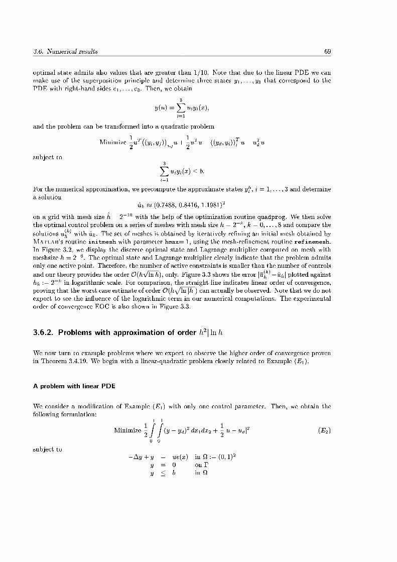
3.6. Numerical results 69
optimal state admits also values that are greater than 1=10. Note that due to the linear PDE we canmake use of the superposition principle and determine three states y1; : : : ; y3 that correspond to thePDE with right-hand sides e1; : : : ; e3. Then, we obtain
y(u) =
3Xi=1
uiyi(x);
and the problem can be transformed into a quadratic problem
Minimize1
2uT�(yi; yj)
�i;ju+
1
2uTu� ((yd; yi))
Ti u� uTd u
subject to3Xi=1
uiyi(x) � b:
For the numerical approximation, we precompute the approximate states yhi , i = 1; : : : ; 3 and determinea solution
uh � (0:7488; 0:8416; 1:1981)T
on a grid with mesh size h = 2�10 with the help of the optimization routine quadprog. We then solvethe optimal control problem on a series of meshes with mesh size h = 2�k, k = 0; : : : ; 8 and compare the
solutions �u(k)h with uh. The set of meshes is obtained by iteratively re�ning an initial mesh obtained by
Matlab's routine initmesh with parameter hmax= 1, using the mesh-re�nement routine refinemesh.In Figure 3.2, we display the discrete optimal state and Lagrange multiplier computed on mesh withmeshsize h = 2�6. The optimal state and Lagrange multiplier clearly indicate that the problem admitsonly one active point. Therefore, the number of active constraints is smaller than the number of controls
and our theory provides the order O(hplnh), only. Figure 3.3 shows the error j�u(k)h �uhj plotted againsthk := 2�k in logarithmic scale. For comparison, the straight line indicates linear order of convergence,proving that the worst case estimate of order O(hpln jhj) can actually be observed. Note that we do notexpect to see the in uence of the logarithmic term in our numerical computations. The experimentalorder of convergence EOC is also shown in Figure 3.3.
3.6.2. Problems with approximation of order h2j lnhj
We now turn to example problems where we expect to observe the higher order of convergence provenin Theorem 3.4.19. We begin with a linear-quadratic problem closely related to Example (E1).
A problem with linear PDE
We consider a modi�cation of Example (E1) with only one control parameter. Then, we obtain thefollowing formulation:
Minimize1
2
1Z0
1Z0
(y � yd)2 dx1dx2 +
1
2ju� udj2 (E2)
subject to��y + y = ue(x) in := (0; 1)2
y = 0 on �y � b in

70 3. An elliptic control problem of semi-in�nite type
Figure 3.2.: Example (E1): Discrete optimal state and Lagrange multiplier
with
yd(x) = (x1 + x21 � 2x31)(x2 + x22 � 2x32); e(x) = e1(x) + e2(x) + e3(x); ud = 1; b =1
10;
cf. (3.6.1){(3.6.4) as well as (3.6.5). Again, the exact solution of this problem is not known, and wetherefore compute a reference solution
uh � 0:35849
on a �ne grid with mesh size h = 2�10 and proceed as before. We calculate discrete optimal solutionson a set of iteratively re�ned meshes with mesh size hk = 2�k, 0 = 1; : : : ; 9, where we again precomputea state yhe that solves the PDE with right-hand side e(x). We then obtain �yh = �uh � yhe . Figure 3.4shows the optimal state and Lagrange multiplier computed on a mesh with h = 2�6. Figure 3.5 showsthe error in the optimal control, indicating quadratic convergence, both in numbers and graphically.
Comparison of Examples (E1) and (E2)
Before we continue with a further example involving a nonlinear PDE we brie y compare Example (E1)and (E2). Both have been constructed in a similar manner. Example (E1) admits three controls u1,
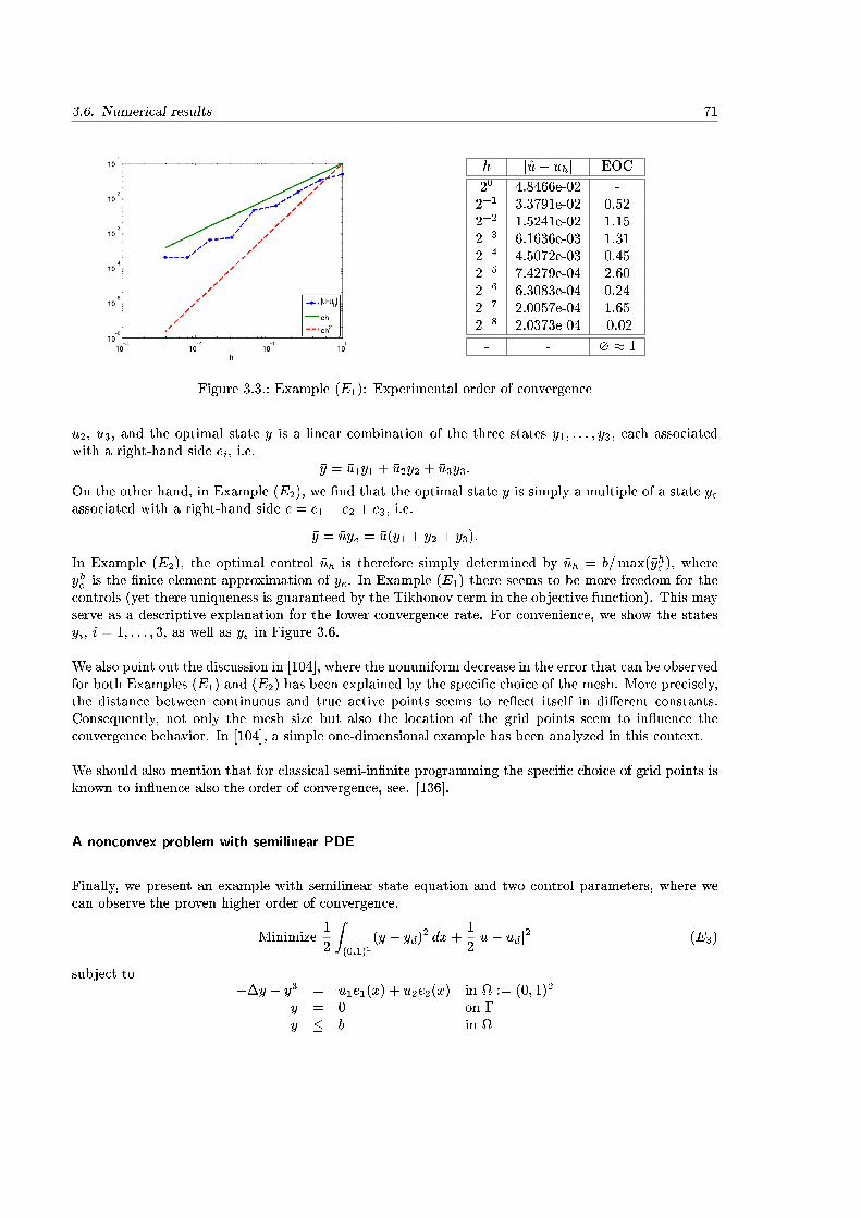
3.6. Numerical results 71
h ju� �uhj EOC
20 4.8466e-02 -2�1 3.3791e-02 0.522�2 1.5241e-02 1.152�3 6.1636e-03 1.312�4 4.5072e-03 0.452�5 7.4279e-04 2.602�6 6.3083e-04 0.242�7 2.0057e-04 1.652�8 2.0373e-04 -0.02
- - ? � 1
Figure 3.3.: Example (E1): Experimental order of convergence
u2, u3, and the optimal state �y is a linear combination of the three states y1; : : : ; y3, each associatedwith a right-hand side ei, i.e.
�y = �u1y1 + �u2y2 + �u3y3:
On the other hand, in Example (E2), we �nd that the optimal state �y is simply a multiple of a state yeassociated with a right-hand side e = e1 + e2 + e3, i.e.
�y = �uye = �u(y1 + y2 + y3):
In Example (E2), the optimal control �uh is therefore simply determined by �uh = b=max(�yhe ), whereyhe is the �nite element approximation of ye. In Example (E1) there seems to be more freedom for thecontrols (yet there uniqueness is guaranteed by the Tikhonov term in the objective function). This mayserve as a descriptive explanation for the lower convergence rate. For convenience, we show the statesyi, i = 1; : : : ; 3, as well as ye in Figure 3.6.
We also point out the discussion in [104], where the nonuniform decrease in the error that can be observedfor both Examples (E1) and (E2) has been explained by the speci�c choice of the mesh. More precisely,the distance between continuous and true active points seems to re ect itself in di�erent constants.Consequently, not only the mesh size but also the location of the grid points seem to in uence theconvergence behavior. In [104], a simple one-dimensional example has been analyzed in this context.
We should also mention that for classical semi-in�nite programming the speci�c choice of grid points isknown to in uence also the order of convergence, see. [136].
A nonconvex problem with semilinear PDE
Finally, we present an example with semilinear state equation and two control parameters, where wecan observe the proven higher order of convergence.
Minimize1
2
Z(0;1)2
(y � yd)2 dx+
1
2ju� udj2 (E3)
subject to��y + y3 = u1e1(x) + u2e2(x) in := (0; 1)2
y = 0 on �y � b in
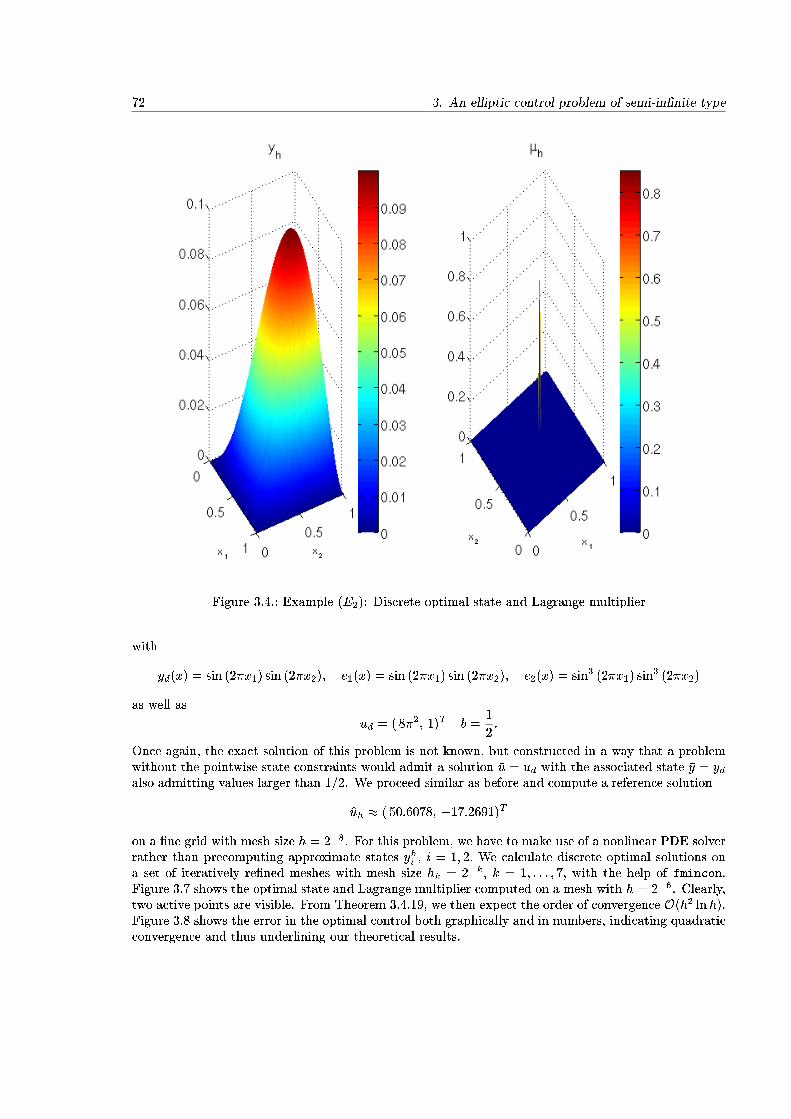
72 3. An elliptic control problem of semi-in�nite type
Figure 3.4.: Example (E2): Discrete optimal state and Lagrange multiplier
with
yd(x) = sin (2�x1) sin (2�x2); e1(x) = sin (2�x1) sin (2�x2); e2(x) = sin3 (2�x1) sin3 (2�x2)
as well as
ud = ( 8�2; 1)T b =1
2:
Once again, the exact solution of this problem is not known, but constructed in a way that a problemwithout the pointwise state constraints would admit a solution �u = ud with the associated state �y = ydalso admitting values larger than 1=2. We proceed similar as before and compute a reference solution
uh � ( 50:6078; �17:2691)T
on a �ne grid with mesh size h = 2�8. For this problem, we have to make use of a nonlinear PDE solverrather than precomputing approximate states yhi , i = 1; 2: We calculate discrete optimal solutions ona set of iteratively re�ned meshes with mesh size hk = 2�k, k = 1; : : : ; 7, with the help of fmincon.Figure 3.7 shows the optimal state and Lagrange multiplier computed on a mesh with h = 2�6. Clearly,two active points are visible. From Theorem 3.4.19, we then expect the order of convergence O(h2 lnh).Figure 3.8 shows the error in the optimal control both graphically and in numbers, indicating quadraticconvergence and thus underlining our theoretical results.
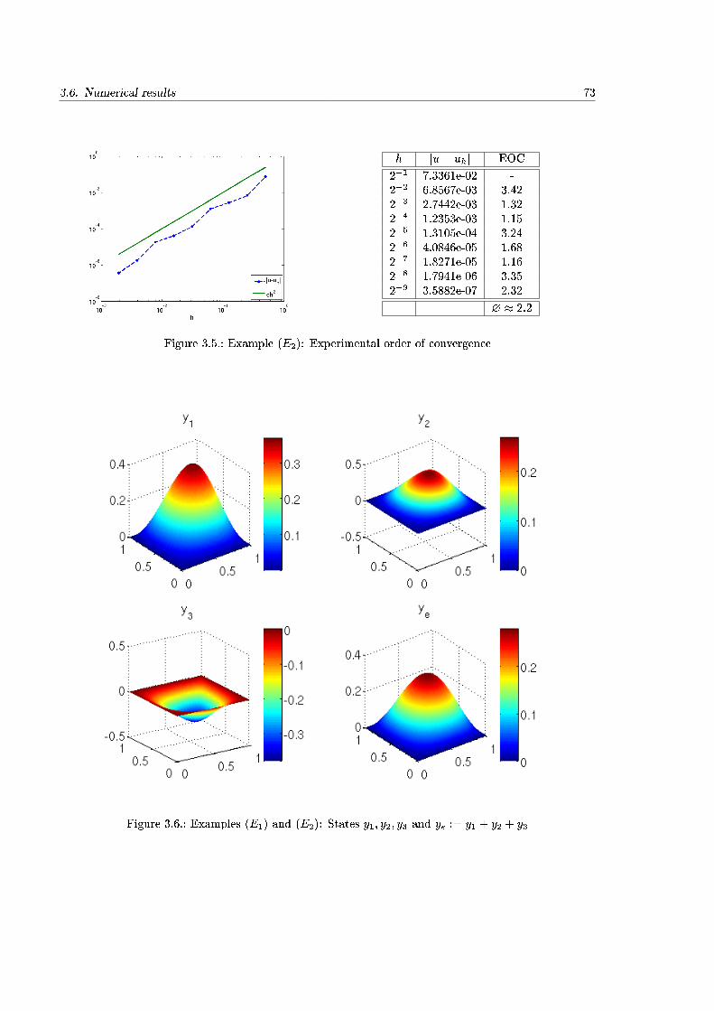
3.6. Numerical results 73
h j�u� �uhj EOC
2�1 7.3361e-02 -2�2 6.8567e-03 3.422�3 2.7442e-03 1.322�4 1.2353e-03 1.152�5 1.3105e-04 3.242�6 4.0846e-05 1.682�7 1.8271e-05 1.162�8 1.7941e-06 3.352�9 3.5882e-07 2.32
- - ? � 2:2
Figure 3.5.: Example (E2): Experimental order of convergence
Figure 3.6.: Examples (E1) and (E2): States y1; y2; y3 and ye := y1 + y2 + y3
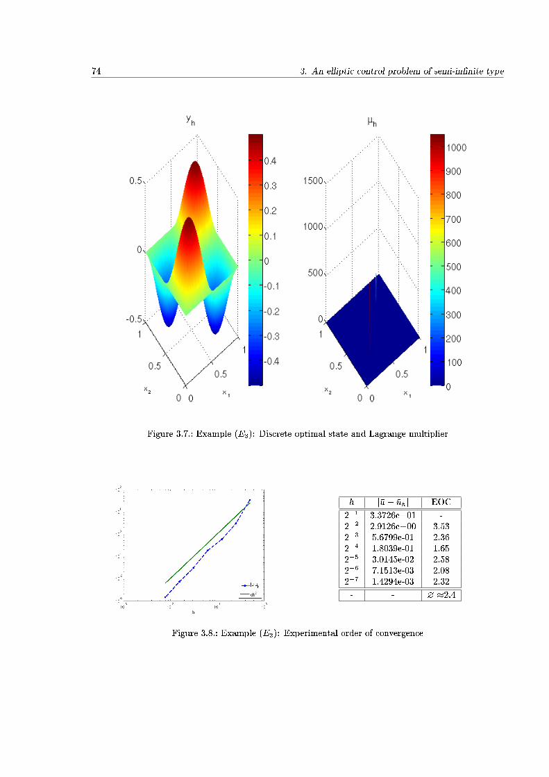
74 3. An elliptic control problem of semi-in�nite type
Figure 3.7.: Example (E3): Discrete optimal state and Lagrange multiplier
h j�u� �uhj EOC
2�1 3.3726e+01 -2�2 2.9126e+00 3.532�3 5.6799e-01 2.362�4 1.8039e-01 1.652�5 3.0145e-02 2.582�6 7.1513e-03 2.082�7 1.4294e-03 2.32
- - ? �2.4
Figure 3.8.: Example (E3): Experimental order of convergence

4. A parabolic control problem with pointwise
state and control constraints
4.1. Introduction
We now consider a model problem governed by a semilinear parabolic PDE and spatio-temporal controlfunctions, subject to pointwise bounds on the state and the control. In the introduction and in the lastchapter we have already discussed how pointwise state constraints present a challenge in the analysisof PDE-constrained optimal control problems. Compared to the semi-in�nite problem (3.1.1) we nowobserve additional challenges. First, we now deal with control functions rather than �nitely manycontrol parameters. From the analytic point of view, the parabolic initial-boundary value problemdemands higher regularity of the given data for comparable regularity results for the states. Due tothe presence of pointwise bounds on the control, we have at least su�cient regularity of the states for ameaningful discussion of �rst order necessary optimality conditions, yet only limited results on secondorder su�cient conditions are available. From the viewpoint of �nite element error estimates additionalchallenges come into play which we will comment on in more detail in the next chapter.
For these reasons we do not aim directly at proving error estimates for a �nite element discretization,but discuss a regularization of the problem �rst. Let us give a brief overview about three regularizationmethods that have been studied frequently in the recent past. A �rst approach is the Moreau-Yosidatype regularization method by Ito and Kunisch [78], where the pointwise state constraints
ya � y � yb
are penalized by a quadratic penalty functional and a regularized control constrained problem is ob-tained. The resulting objective function in its simplest form contains terms of the type
1
2
ZZQ
max(0; (y � yb))2 dxdt+
1
2
ZZQ
max(0; (ya � y ))2 dxdt
added to the unregularized objective function J(y; u), where denotes a regularization parameter thatis chosen large. After di�erentiation, this leads to a nondi�erentiable term
max(0; y � yb)� max(0; ya � y )
in the right-hand side of the adjoint equation. A semi-smooth Newton approach has proven to workwell in numerical computations, and allows a function space analysis of this problem, cf. [78]. However,since the objective function is not twice di�erentiable, a classical second-order analysis is not possible. Aworkaround has recently been presented by Krumbiegel, R�osch, and the author in [84]; we will commenton this shortly.
Later, Meyer, R�osch, and Tr�oltzsch, cf. [110], suggested a Lavrentiev type method that in some sensepreserves the nature of state-constraints, replacing them by mixed control-state constraints
ya � �u+ y � yb;
75
76 4. A parabolic control problem with pointwise state and control constraints
where the regularization parameter � is chosen small. We refer also to the nonlinear setting in [111].Note that this method requires the control and state to be de�ned on the same sets. In e.g. boundarycontrol problems, it cannot directly be applied. A possible extension was proven by Tr�oltzsch and theauthor in [116] for parabolic problems, and by Tr�oltzsch and Yousept, in [145, 146] for elliptic boundarycontrol problems. We will focus in detail on Lavrentiev regularization for distributed control problemsin this thesis.
A third regularization technique developed in the recent past is the virtual control concept by Krumbiegeland R�osch, cf. [85] originally developed for boundary control problems that has also proven useful fordistributed control problems with additional control constraints, cf. [30]. This concept also transferspure state constraints into mixed control-state constraints
ya � "v + y � yb;
but in contrast to Lavrentiev regularization this is done for an additional distributed control, that mayor may not enter the PDE as a source term. To the author's knowledge, there are no publicationsrelated to parabolic problems available.
All techniques have been discussed in more or less detail in the literature, with the main focus onelliptic problems with linear state equation and quadratic objective functional. Special emphasis waslaid on the convergence analysis for the regularization parameter tending to the limit, cf. also theoverview in Chapter 1. Not so many contributions were devoted to this issue in the nonlinear case.We mention [72], where some related questions for the Lavrentiev type regularization in the semilinearelliptic case are discussed, [31], where in addition a regularization error estimate has been proven, and[112], where the convergence of the Moreau-Yosida type regularization has been studied for a semilinearelliptic problem that arises from the control of the growth of SiC bulk single crystals. Convergencefor the Moreau-Yosida regularization for control problems governed by semilinear parabolic equationshas been studied by Tr�oltzsch and the author in [115]. For the virtual control concept, a contributionto the analysis of problems governed by semilinear elliptic equations has recently been published byKrumbiegel, R�osch, and the author, which not only focuses on convergence but also on second-ordersu�cient conditions, cf. [83]. For mixed pointwise control-state constraints, SSC have �rst been studiedby R�osch and Tr�oltzsch et. al. in [133] for elliptic problems, and even earlier for mixed constraints ofbottleneck type in [131].
To put the three regularization approaches into perspective, we point out the known fact that Lavrentievregularization with a virtual control that does not enter the PDE itself, is equivalent to the penalizationmethod by Ito and Kunisch. This fact has recently been used by Krumbiegel, R�osch, and the authorto derive su�cient optimality conditions for the formally less regular Moreau-Yosida regularization inan elliptic setting, cf. [84]. When comparing the virtual control concept with classical Lavrentievregularization, it stands out that the virtual control approach keeps the control constraints separatefrom the mixed control-state constraints, i.e. one obtains
ua � u � ub; ya � "v + y � yb; (4.1.1)
where u and y do not appear in the same inequality. In contrast, for Lavrentiev regularization with
ua � u � ub; ya � �u+ y � yb; (4.1.2)
the control appears by itself in the control constraints and together with the state in the mixed control-state constraints. We will comment on some consequences of this di�erence between Lavrentiev typeregularization and the virtual control concept later on.
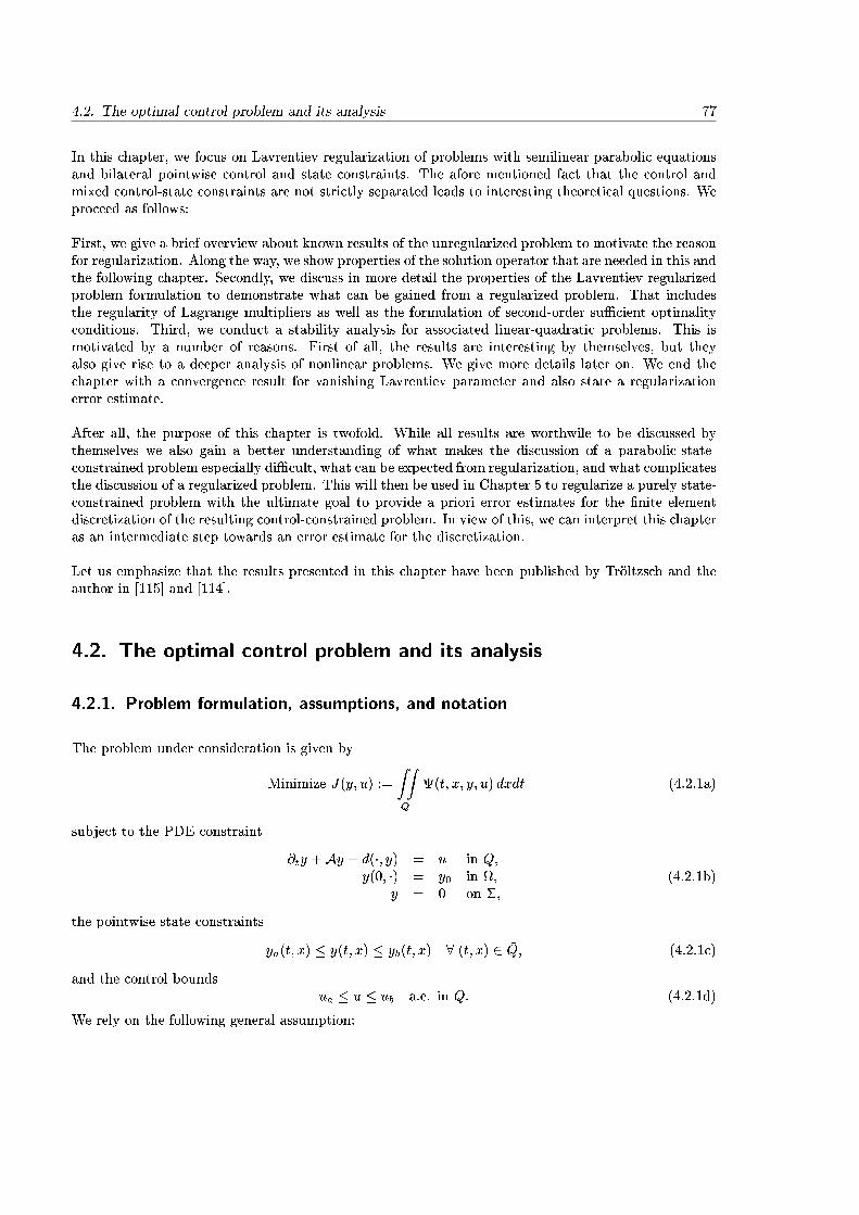
4.2. The optimal control problem and its analysis 77
In this chapter, we focus on Lavrentiev regularization of problems with semilinear parabolic equationsand bilateral pointwise control and state constraints. The afore mentioned fact that the control andmixed control-state constraints are not strictly separated leads to interesting theoretical questions. Weproceed as follows:
First, we give a brief overview about known results of the unregularized problem to motivate the reasonfor regularization. Along the way, we show properties of the solution operator that are needed in this andthe following chapter. Secondly, we discuss in more detail the properties of the Lavrentiev-regularizedproblem formulation to demonstrate what can be gained from a regularized problem. That includesthe regularity of Lagrange multipliers as well as the formulation of second-order su�cient optimalityconditions. Third, we conduct a stability analysis for associated linear-quadratic problems. This ismotivated by a number of reasons. First of all, the results are interesting by themselves, but theyalso give rise to a deeper analysis of nonlinear problems. We give more details later on. We end thechapter with a convergence result for vanishing Lavrentiev parameter and also state a regularizationerror estimate.
After all, the purpose of this chapter is twofold. While all results are worthwile to be discussed bythemselves we also gain a better understanding of what makes the discussion of a parabolic-state-constrained problem especially di�cult, what can be expected from regularization, and what complicatesthe discussion of a regularized problem. This will then be used in Chapter 5 to regularize a purely state-constrained problem with the ultimate goal to provide a priori error estimates for the �nite elementdiscretization of the resulting control-constrained problem. In view of this, we can interpret this chapteras an intermediate step towards an error estimate for the discretization.
Let us emphasize that the results presented in this chapter have been published by Tr�oltzsch and theauthor in [115] and [114].
4.2. The optimal control problem and its analysis
4.2.1. Problem formulation, assumptions, and notation
The problem under consideration is given by
Minimize J(y; u) :=
ZZQ
(t; x; y; u) dxdt (4.2.1a)
subject to the PDE constraint
@ty +Ay + d(�; y) = u in Q;y(0; �) = y0 in ;
y = 0 on �;(4.2.1b)
the pointwise state constraints
ya(t; x) � y(t; x) � yb(t; x) 8 (t; x) 2 �Q; (4.2.1c)
and the control boundsua � u � ub a.e. in Q: (4.2.1d)
We rely on the following general assumption:

78 4. A parabolic control problem with pointwise state and control constraints
Assumption 4.2.1.
(A.1) Let Assumption 2.3.1 on page 19 hold, and let the di�erential operator A satisfy (2.3.3) and (2.3.4)on page 19. Moreover, let the nonlinearity d ful�ll the conditions stated in Assumption 2.5.3.
(A.2) The initial state y0 is a function from C(�) \ H10 (). The constraints on the control and state
are given by ua; ub 2 L1(Q), ub � ua � c > 0 a.e. in Q, and ya; yb 2 C( �Q), ya � yb in �Q,respectively, such that ya(x; 0) < y0(x) < yb(x; 0) holds for all x 2 �. We additionally assumeya(t; x) < 0 < yb(t; x) for all (t; x) 2 �, as well as y0(x; 0) = 0 on �.
(A.3) The function = (t; x; y; u) : Q�R�R! R ful�lls Assumption 2.2.3, i.e. it is measurable withrespect to (t; x) 2 Q for all �xed (y; u) 2 R2, and twice continuously di�erentiable with respect to(y; u) for almost all (t; x) 2 Q. Its �rst and second order derivative will be denoted by 0 and00, respectively. Moreover, for y = u = 0, the function , and its derivatives up to order twoare bounded and Lipschitz continuous on bounded sets with respect to y and u, i.e. they ful�llconditions (2.2.1) and (2.2.2) accordingly.
(A.4) Moreover, the function is assumed to ful�ll the Legendre-Clebsch condition
@uu(t; x; y; u) � �0 > 0 (4.2.2)
for almost all (t; x) 2 Q, all y 2 R, and all u 2 [inf ua; supub].
(A.5) Last, is convex in u, i.e.
(t; x; y; �u+ (1� �)v) � �(t; x; y; u) + (1� �)(t; x; y; v)
for almost all (t; x) 2 Q, all u; v 2 R, and every � 2 (0; 1).
The general representation of the objective function has immediate consequences when discussing e.g.the di�erentiability or Lipschitz continuity properties, which a�ects for instance the discussion of secondorder su�cient conditions for the optimal control problem and its regularized version to be discussed inthe next chapter. In particular, we will generally not obtain L2-di�erentiability of the objective functionwith respect to u.
Last, we again agree that V := H10 () and Y :=W(0; T ) is given, and for short notation we introduce
the control spaceU := L1(Q)
and the set of admissible controls
Uad := fu 2 L1(Q) : ua � u � ubg:We will also use the general notation introduced in Chapter 2 and in particular point out the shortnotation (2.5.1) on page 23 for some frequently appearing norms. In the remainder of this section,we proceed as in the elliptic case. We introduce a control-to-state operator and a reduced objectivefunction, and with the help of their properties discuss the existence of optimal solutions, as well as �rstand second order optimality conditions.
4.2.2. The control-to-state operator and the reduced objective functional
The state equation (4.2.1b) �ts into the general setting of the initial-boundary value problem (2.3.2)discussed in Chapter 2. Hence, Theorem 2.5.6 ensures that the following de�nition is meaningful:

4.2. The optimal control problem and its analysis 79
De�nition 4.2.2. The mapping
G : U !W(0; T ) \ C( �Q); u 7! y = G(u);
where y solves (4.2.1b) in weak sense, is called the control-to-state-operator associated with Problem(4.2.1). In addition, we introduce the reduced objective functional
f : U ! R; f(u) := J(G(u); u):
We proceed by collecting di�erentiability properties of G and f .
Proposition 4.2.3. The control-to-state-operator G is of class C2. Let v; v1; v2 2 L1(Q) and y = G(u)be given. Then, the �rst and second order derivatives of G are given by ~y := G0(u)v and ~z := G00(u)v1v2being the solutions of
@t~y +A~y + @yd(�; y)~y = v in Q~y(0; �) = 0 in
~y = 0 on �;(4.2.3)
@t~z +A~z + @yd(�; y)~z = �@yyd(�; y)~y1~y2 in Q~z(0; �) = 0 in
~z = 0 on �:(4.2.4)
where ~y1 = G0(u)v1 and ~y2 = G0(u)v2. The reduced objective function f is of class C2 with respect tothe L1-topology. For u; v; v1; v2 2 L1 and ~yi := G0(u)vi, i = 1; 2, as well as z = G00(u)[v1; v2] its �rstand second order derivative are given by
f 0(u)v =
ZZQ
(@y(t; x; y; u)~y + @u(t; x; y; u)v) dxdt
f 00(u)[v1; v2] =
ZZQ
�~y1v1
�T �@yy(t; x; y; u) @yu(t; x; y; u)@uy(t; x; y; u) @uu(t; x; y; u)
� �~y2v2
�dxdt
+
ZZQ
@y(t; x; y; u)z dxdt:
Proof. For the di�erentiability of G, we refer to Theorems 5.9, 5.15, and 5.16 in [144]. Moreover, by[144, Lemma 4.12], we know that the objective function J : L1(Q)�L1(Q)! R is twice continuouslydi�erentiable. Then, by the properties of G and the chain rule, the assertion is obtained.
The estimates from Proposition 2.5.2 hold for ~y and ~z, since @yd(�; y) is bounded by Assumption 4.2.1.The following Lipschitz stability results will be helpful in the sequel.
Lemma 4.2.4. Let u1; u2 2 Uad and v 2 L1(Q) be given. Then there exists a constant C > 0 suchthat
kG(u1)�G(u2)kL2(Q)\L1(I;V ) �C ku1 � u2kI (4.2.5)
kG(u1)�G(u2)k1;1 �C ku1 � u2kLp(Q) (4.2.6)
kG0(u1)v �G0(u2)vkI �C ku1 � u2kIkvkI (4.2.7)
kG0(u1)v �G0(u2)vk1;1 �C ku1 � u2k1;1kvkLp(Q) (4.2.8)
kG00(u1)[v; v]�G00(u2)[v; v]kI �C ku1 � u2kIkvk2I (4.2.9)
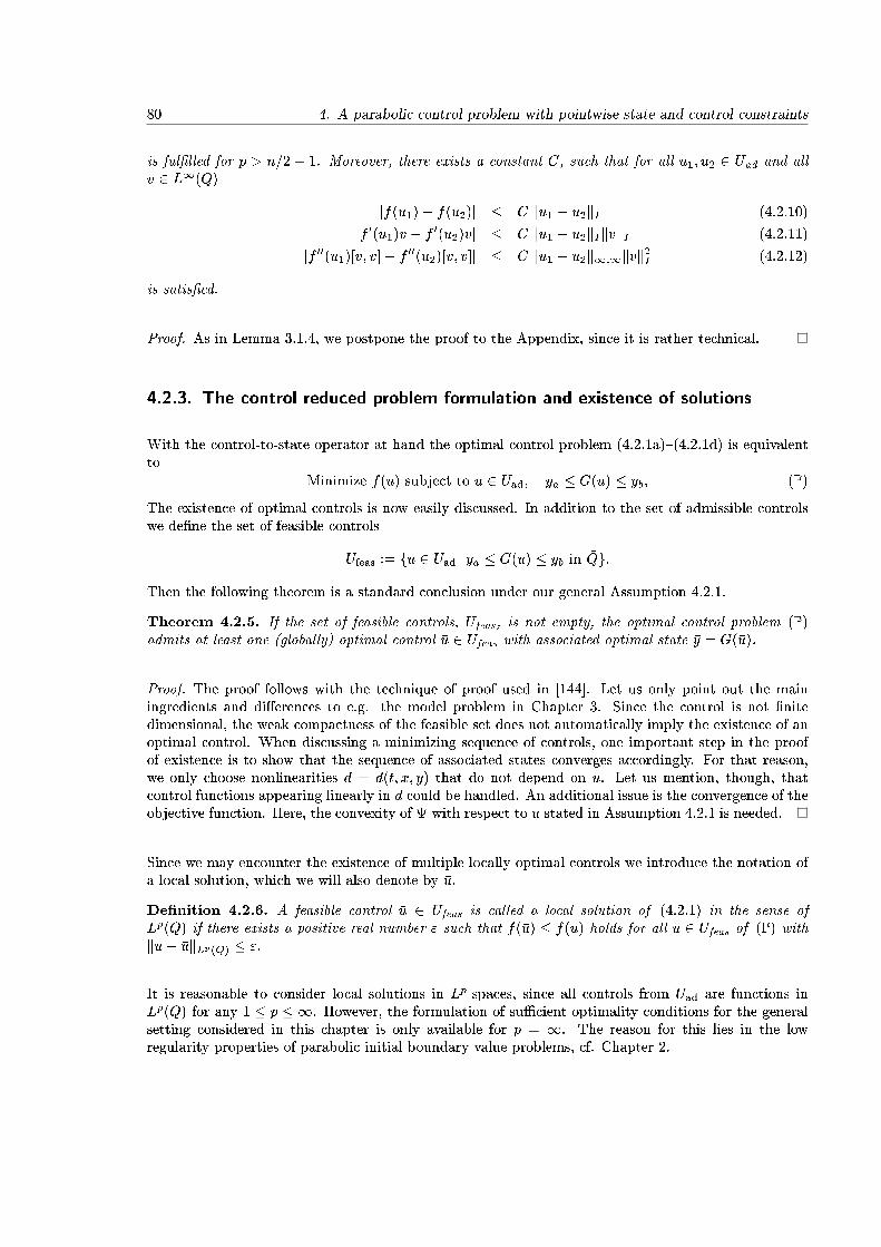
80 4. A parabolic control problem with pointwise state and control constraints
is ful�lled for p > n=2 + 1. Moreover, there exists a constant C, such that for all u1; u2 2 Uad and allv 2 L1(Q)
jf(u1)� f(u2)j � C ku1 � u2kI (4.2.10)
jf 0(u1)v � f 0(u2)vj � C ku1 � u2kIkvkI (4.2.11)
jf 00(u1)[v; v]� f 00(u2)[v; v]j � C ku1 � u2k1;1kvk2I (4.2.12)
is satis�ed.
Proof. As in Lemma 3.1.4, we postpone the proof to the Appendix, since it is rather technical.
4.2.3. The control reduced problem formulation and existence of solutions
With the control-to-state operator at hand the optimal control problem (4.2.1a){(4.2.1d) is equivalentto
Minimize f(u) subject to u 2 Uad; ya � G(u) � yb; (P)
The existence of optimal controls is now easily discussed. In addition to the set of admissible controlswe de�ne the set of feasible controls
Ufeas := fu 2 Uad j ya � G(u) � yb in �Qg:
Then the following theorem is a standard conclusion under our general Assumption 4.2.1.
Theorem 4.2.5. If the set of feasible controls, Ufeas, is not empty, the optimal control problem (P)admits at least one (globally) optimal control �u 2 Ufeas with associated optimal state �y = G(�u).
Proof. The proof follows with the technique of proof used in [144]. Let us only point out the mainingredients and di�erences to e.g. the model problem in Chapter 3. Since the control is not �nitedimensional, the weak compactness of the feasible set does not automatically imply the existence of anoptimal control. When discussing a minimizing sequence of controls, one important step in the proofof existence is to show that the sequence of associated states converges accordingly. For that reason,we only choose nonlinearities d = d(t; x; y) that do not depend on u. Let us mention, though, thatcontrol functions appearing linearly in d could be handled. An additional issue is the convergence of theobjective function. Here, the convexity of with respect to u stated in Assumption 4.2.1 is needed.
Since we may encounter the existence of multiple locally optimal controls we introduce the notation ofa local solution, which we will also denote by �u.
De�nition 4.2.6. A feasible control �u 2 Ufeas is called a local solution of (4.2.1) in the sense ofLp(Q) if there exists a positive real number " such that f(�u) � f(u) holds for all u 2 Ufeas of (P) withku� �ukLp(Q) � ":
It is reasonable to consider local solutions in Lp-spaces, since all controls from Uad are functions inLp(Q) for any 1 � p � 1. However, the formulation of su�cient optimality conditions for the generalsetting considered in this chapter is only available for p = 1. The reason for this lies in the lowregularity properties of parabolic initial boundary value problems, cf. Chapter 2.
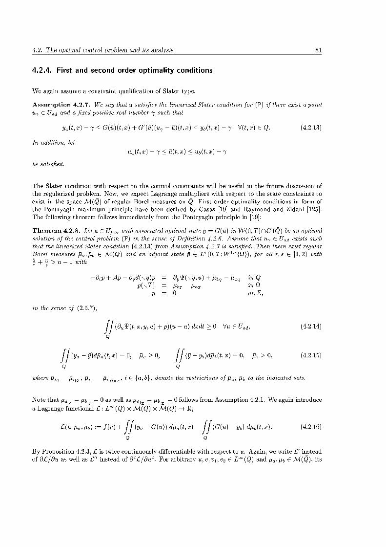
4.2. The optimal control problem and its analysis 81
4.2.4. First and second order optimality conditions
We again assume a constraint quali�cation of Slater type.
Assumption 4.2.7. We say that �u satis�es the linearized Slater condition for (P) if there exist a pointu 2 Uad and a �xed positive real number such that
ya(t; x) + � G(�u)(t; x) +G0(�u)(u � �u)(t; x) � yb(t; x)� 8(t; x) 2 �Q: (4.2.13)
In addition, let
ua(t; x) + � �u(t; x) � ub(t; x)�
be satis�ed.
The Slater condition with respect to the control constraints will be useful in the future discussion ofthe regularized problem. Now, we expect Lagrange multipliers with respect to the state constraints toexist in the space M( �Q) of regular Borel measures on �Q. First order optimality conditions in form ofthe Pontryagin maximum principle have been derived by Casas [19] and Raymond and Zidani [125].The following theorem follows immediately from the Pontryagin principle in [19]:
Theorem 4.2.8. Let �u 2 Ufeas with associated optimal state �y = G(�u) in W(0; T )\C ( �Q) be an optimalsolution of the control problem (P) in the sense of De�nition 4.2.6. Assume that u 2 Uad exists suchthat the linearized Slater condition (4.2.13) from Assumption 4.2.7 is satis�ed. Then there exist regularBorel measures ��a; ��b 2 M( �Q) and an adjoint state �p 2 Lr(0; T ;W 1;s()), for all r; s 2 [1; 2) with2r +
ns > n+ 1 with
�@t�p+A�p+ @yd(�; �y)�p = @y(�; �y; �u) + ��bQ � ��aQ in Q�p(�; T ) = ��bT � ��aT in
�p = 0 on �;
in the sense of (2.5.7), ZZQ
(@u(t; x; �y; �u) + �p)(u� �u) dxdt � 0 8u 2 Uad; (4.2.14)
ZZ�Q
(ya � �y)d��a(t; x) = 0; ��a � 0;
ZZ�Q
(�y � yb)d��b(t; x) = 0; ��b � 0; (4.2.15)
where ��iQ = ��ijQ , ��iT = ��ij��T ; i 2 fa; bg, denote the restrictions of ��a, ��b to the indicated sets.
Note that ��aj0 = ��bj0 = 0 as well as ��aj� = ��bj� = 0 follows from Assumption 4.2.1. We again introduce
a Lagrange functional L : L1(Q)�M( �Q)�M( �Q)! R,
L(u; �a; �b) := f(u) +
ZZ�Q
(ya �G(u)) d�a(t; x) +
ZZ�Q
(G(u)� yb) d�b(t; x): (4.2.16)
By Proposition 4.2.3, L is twice continuously di�erentiable with respect to u. Again, we write L0 insteadof @L=@u as well as L00 instead of @2L=@u2. For arbitrary u; v; v1; v2 2 L1(Q) and �a; �b 2 M( �Q), its

82 4. A parabolic control problem with pointwise state and control constraints
�rst and second order derivatives can be determined to ful�ll
L0(u; �a; �b)v = f 0(u)v �ZZ�Q
G0(u)v d�a(t; x) +
ZZ�Q
G0(u)v d�b(t; x)
=
ZZ�Q
(@u(t; x; y; u)v + pv) dxdt
L00(u; �a; �b)[v1; v2] = f 00(u)[v1; v2]�ZZ�Q
G00(u)[v1; v2] d�a(t; x) +
ZZ�Q
G00(u)[v1; v2] d�b(t; x)
=
ZZQ
�~y1v1
�T �@yy(t; x; y; u) @yu(t; x; y; u)@uy(t; x; y; u) @uu(t; x; y; u)
� �~y2v2
�dxdt
�ZZQ
p@yyd(t; x; y)[~y1; ~y2] dxdt;
where p solves (4.2.14). We refer to [144] for a detailed discussion.
Now, Theorem 4.2.8 is equivalent to the existence of nonnegative Lagrange multipliers ��a; ��b 2 M( �Q)such that
L0(�u; ��a; ��b)(u� �u) � 0 8 u 2 Uad (4.2.17)
and ZZ�Q
(ya �G(�u)) d��a(t; x) =
ZZ�Q
(G(�u)� yb) d��b(t; x) = 0: (4.2.18)
Due to the nonconvexity of the problem it is desirable to consider the formulation of second ordersu�cient optimality conditions. There are very few publications concerned with parabolic problemswith pure pointwise state constraints. For unregularized parabolic semilinear problems, SSC have onlybeen proven in full generality for one-dimensional distributed control, cf. [123] and [22]. For higherdimensions, SSC have been established in the special setting with �nitely many time-dependent controlsin the recent work [36].
Assumption 4.2.9. Let �u 2 Uad be a control satisfying the �rst order necessary optimality conditionsof Theorem 4.2.8 and let ��a; ��b be Lagrange multipliers with respect to the state constraints (4.2.1c).We assume that there exists a constant � > 0, such that
@2L@u2
(�u; ��a; ��b)[v; v] � �kvk2Iis valid for all v 2 L1(Q).
Just as in the elliptic setting it is a quite strong requirement to demand this de�niteness property forall directions v 2 L1(Q), and it is possible to weaken this assumption along the lines of [36]. However,there are dimensional restrictions that apply even in this setting.
The following result is a consequence of Lemma 4.2.4. It will be helpful in the sequel and at the sametime demonstrate the dimensional limits in the parabolic setting.
Corollary 4.2.10. Let the space dimension n be equal to one. For all �xed �a; �b 2 M( �Q), arbitraryu1; u2 2 Uad and v 2 L1(Q), there exists a constant C > 0 such that
jL00(u1; �a; �b)[v; v]� L00(u2; �a; �b)[v; v]j � Cku1 � u2k1;1kvk2I :

4.2. The optimal control problem and its analysis 83
Proof. Due to Lemma 4.2.4, we only need to consider the terms associated with the Lagrange multipliers.Observe that�������
ZZ�Q
(G00(u1)�G00(u2)) [v; v] d�a(t; x)
������� � ck (G00(u1)�G00(u2)) [v; v]kC( �Q)k�akM(Q)
� ck (G00(u1)�G00(u2)) [v; v]kC( �Q)
since �a is �xed. Now, since n = 1, we obtain
k(G00(u1)�G00(u2))[v; v]kC( �Q) � cku1 � u2kIkvk2I ;as in Lemma 4.2.4, and the assertion is obtained after an analogous discussion of the term containing�b.
Let us point out that for higher spatial dimensions, p = 2 is not su�cient for estimation of the C( �Q)norms. In view of second-order su�cient conditions, choosing stronger norms for v is not satisfactory,either.
Theorem 4.2.11. Let n = 1 be satis�ed and let the control �u 2 Ufeas and the Lagrange multipliers��a; ��b ful�ll the conditions stated in Assumption 4.2.9. Then there exist constants � > 0 and " > 0such that
f(�u) � f(u)� �ku� �uk2Iis satis�ed for all u 2 Ufeas with ku� �uk1;1 � ".
Proof. The steps of the proof are the same as in the elliptic setting in Theorem 5.3.12. Note that bythe feasibility of u, the positivity of ��a and ��b and the complementary slackness conditions (4.2.18)from Theorem 4.2.8 we haveZZ
�Q
(G(u)� yb) d��b(t; x)�ZZ�Q
(ya �G(u)) d��a(t; x) � 0;
and ZZ�Q
(G(�u)� yb) d��b(t; x)�ZZ�Q
(ya �G(�u)) d��a(t; x) = 0;
and thereforef(�u) = L(�u; ��a; ��b); f(u) � L(u; ��a; ��b):
Consequently, we obtain by Taylor expansion of L in �u
f(�u)� f(u) � L(�u; ��a; ��b)� L(u; ��a; ��b)= �L0(�u; ��a; ��b)(u� �u)� 1
2L00(u�; ��a; ��b)[u� �u; u� �u]
with u� = �u+ �(u� �u) for some � 2 (0; 1). Making use of (4.2.17) and Assumption 5.3.9 we obtain
f(�u)� f(u) � �1
2L00(�u; ��a; ��b)[u� �u; u� �u]� 1
2(L00(�u; ��a; ��b)� L00(u�; ��a; ��b))[u� �u; u� �u]
� ��2ku� �uk2I +
c
2k�u� u�k1;1ku� �uk2I ;
where the last inequality follows from Corollary 4.2.10. The fact that u� � �u = �(u � �u) yields theassertion for ku � �uk1;1 � ". We refer also to the formulation of weaker second order su�cientconditions in [22].
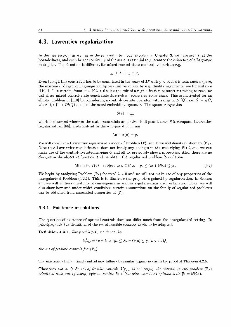
84 4. A parabolic control problem with pointwise state and control constraints
4.3. Lavrentiev regularization
In the last section, as well as in the semi-in�nite model problem in Chapter 3, we have seen that theboundedness, and even better continuity of the state is essential to guarantee the existence of a Lagrangemultiplier. The situation is di�erent for mixed control-state constraints, such as e.g.
ya � �u+ y � yb:
Even though this constraint has to be considered in the sense of Lp with p <1 if u is from such a space,the existence of regular Lagrange multipliers can be shown by e.g. duality arguments, see for instance[110, 142] in certain situations. If � > 0 takes the role of a regularization parameter tending to zero, wecall these mixed control-state constraints Lavrentiev regularized constraints. This is motivated for anelliptic problem in [110] by considering a control-to-state operator with range in L2(Q), i.e. S := i0G,where i0 : Y ! L2(Q) denotes the usual embedding operator. The operator equation
S(u) = yb;
which is observed wherever the state constraints are active, is ill-posed, since S is compact. Lavrentievregularization, [88], leads instead to the well-posed equation
�u+ S(u) = y:
We will consider a Lavrentiev regularized version of Problem (P), which we will denote in short by (P�).Note that Lavrentiev regularization does not imply any changes in the underlying PDE, and we canmake use of the control-to-state-mapping G and all its previously shown properties. Also, there are nochanges in the objective function, and we obtain the regularized problem formulation
Minimize f(u) subject to u 2 Uad; ya � �u+G(u) � yb: (P�)
We begin by analyzing Problem (P�) for �xed � > 0 and we will not make use of any properties of theunregularized Problem (4.2.1). This is to illustrate the properties gained by regularization. In Section4.6, we will address questions of convergence as well as regularization error estimates. Then, we willalso show how and under which conditions certain assumptions on the family of regularized problemscan be obtained from associated properties of (P).
4.3.1. Existence of solutions
The question of existence of optimal controls does not di�er much from the unregularized setting. Inprinciple, only the de�nition of the set of feasible controls needs to be adapted.
De�nition 4.3.1. For �xed � > 0, we denote by
U�feas = fu 2 Uad j ya � �u+G(u) � yb a.e. in Qgthe set of feasible controls for (P�).
The existence of an optimal control now follows by similar arguments as in the proof of Theorem 4.2.5.
Theorem 4.3.2. If the set of feasible controls, U�feas, is not empty, the optimal control problem (P�)admits at least one (globally) optimal control �u� 2 Uad with associated optimal state �y� = G(�u�).
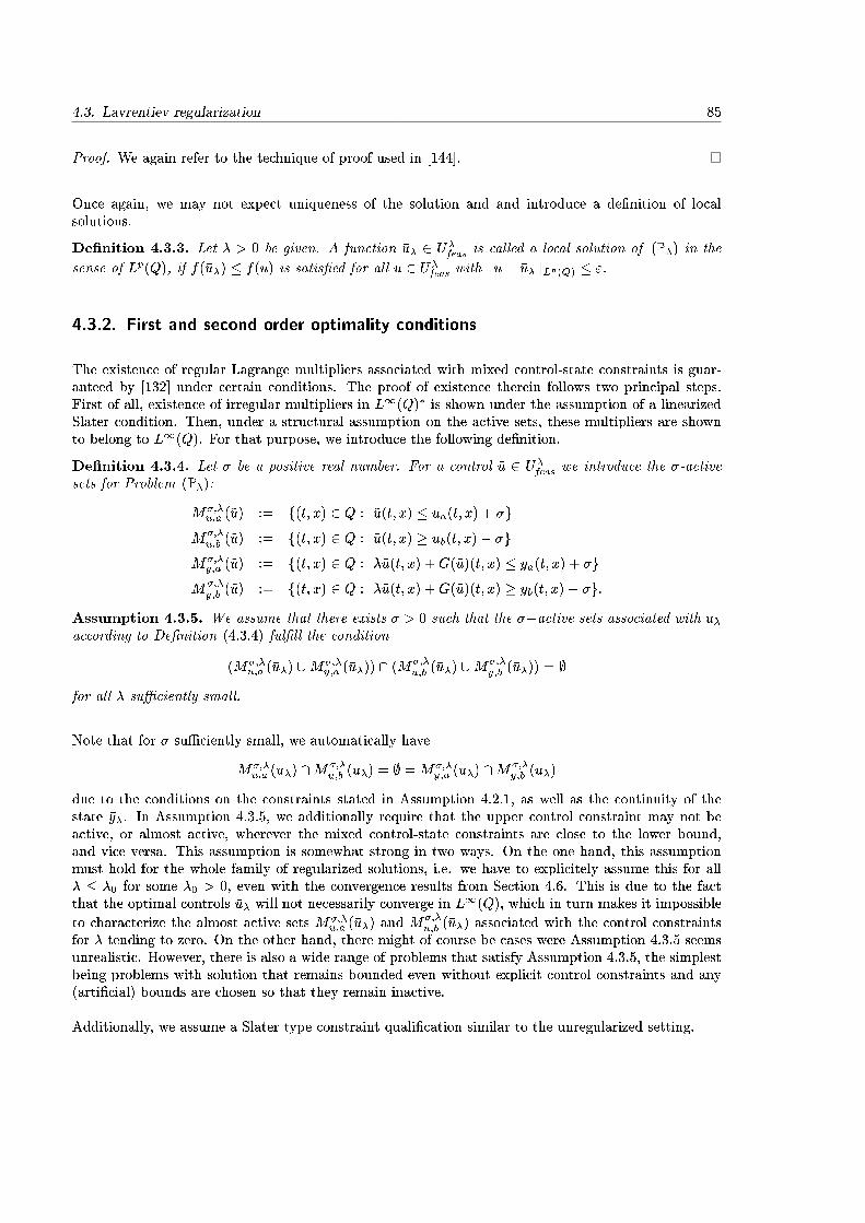
4.3. Lavrentiev regularization 85
Proof. We again refer to the technique of proof used in [144].
Once again, we may not expect uniqueness of the solution and and introduce a de�nition of localsolutions.
De�nition 4.3.3. Let � > 0 be given. A function �u� 2 U�feas is called a local solution of (P�) in the
sense of Lp(Q), if f(�u�) � f(u) is satis�ed for all u 2 U�feas with ku� �u�kLp(Q) � ".
4.3.2. First and second order optimality conditions
The existence of regular Lagrange multipliers associated with mixed control-state constraints is guar-anteed by [132] under certain conditions. The proof of existence therein follows two principal steps.First of all, existence of irregular multipliers in L1(Q)� is shown under the assumption of a linearizedSlater condition. Then, under a structural assumption on the active sets, these multipliers are shownto belong to L1(Q). For that purpose, we introduce the following de�nition.
De�nition 4.3.4. Let � be a positive real number. For a control ~u 2 U�feas we introduce the �-activesets for Problem (P�):
M�;�u;a (~u) := f(t; x) 2 Q : ~u(t; x) � ua(t; x) + �g
M�;�u;b (~u) := f(t; x) 2 Q : ~u(t; x) � ub(t; x)� �g
M�;�y;a (~u) := f(t; x) 2 Q : �~u(t; x) +G(~u)(t; x) � ya(t; x) + �g
M�;�y;b (~u) := f(t; x) 2 Q : �~u(t; x) +G(~u)(t; x) � yb(t; x)� �g:
Assumption 4.3.5. We assume that there exists � > 0 such that the ��active sets associated with �u�according to De�nition (4.3.4) ful�ll the condition
(M�;�u;a (�u�) [M�;�
y;a (�u�)) \ (M�;�u;b (�u�) [M�;�
y;b (�u�)) = ;for all � su�ciently small.
Note that for � su�ciently small, we automatically have
M�;�u;a (�u�) \M�;�
u;b (�u�) = ; =M�;�y;a (�u�) \M�;�
y;b (�u�)
due to the conditions on the constraints stated in Assumption 4.2.1, as well as the continuity of thestate �y�. In Assumption 4.3.5, we additionally require that the upper control constraint may not beactive, or almost active, wherever the mixed control-state constraints are close to the lower bound,and vice versa. This assumption is somewhat strong in two ways. On the one hand, this assumptionmust hold for the whole family of regularized solutions, i.e. we have to explicitely assume this for all� � �0 for some �0 > 0, even with the convergence results from Section 4.6. This is due to the factthat the optimal controls �u� will not necessarily converge in L
1(Q), which in turn makes it impossible
to characterize the almost active sets M�;�u;a (�u�) and M
�;�u;b (�u�) associated with the control constraints
for � tending to zero. On the other hand, there might of course be cases were Assumption 4.3.5 seemsunrealistic. However, there is also a wide range of problems that satisfy Assumption 4.3.5, the simplestbeing problems with solution that remains bounded even without explicit control constraints and any(arti�cial) bounds are chosen so that they remain inactive.
Additionally, we assume a Slater type constraint quali�cation similar to the unregularized setting.
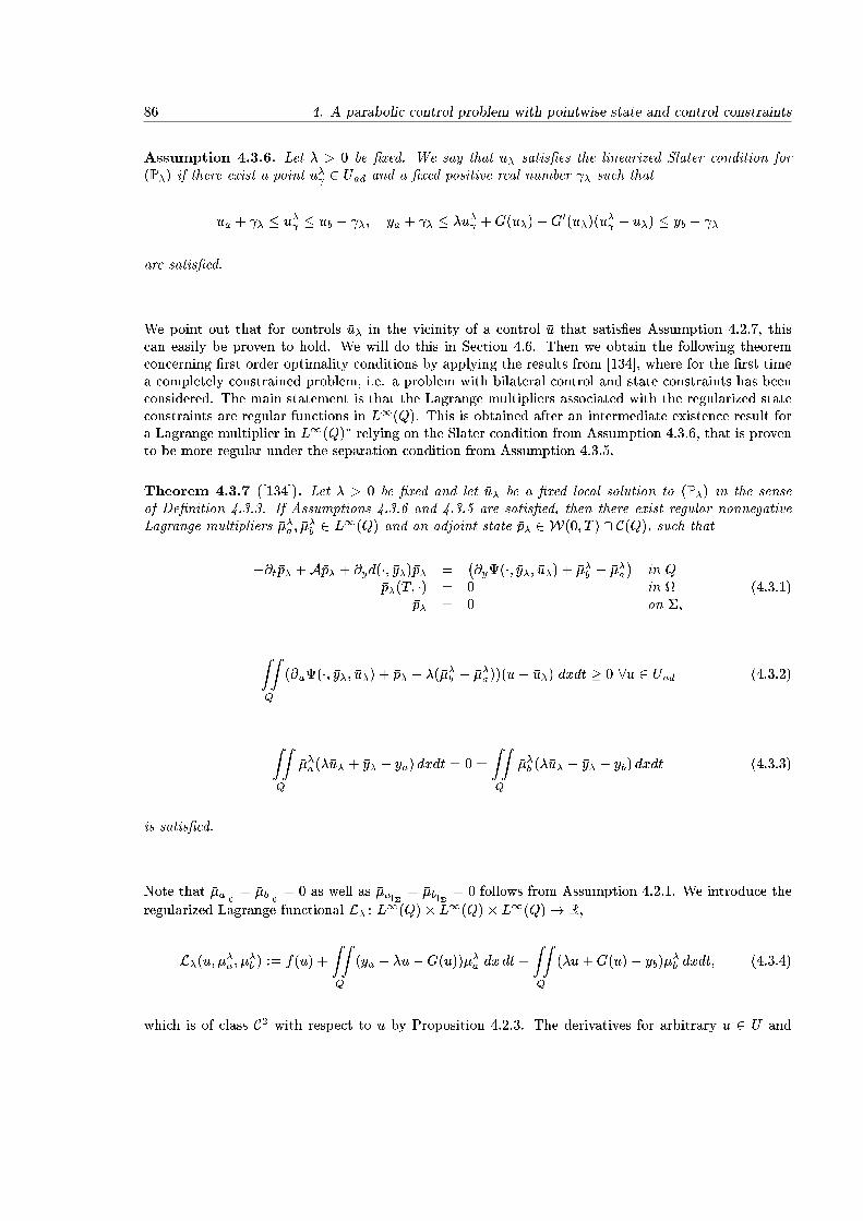
86 4. A parabolic control problem with pointwise state and control constraints
Assumption 4.3.6. Let � > 0 be �xed. We say that �u� satis�es the linearized Slater condition for(P�) if there exist a point u� 2 Uad and a �xed positive real number � such that
ua + � � u� � ub � �; ya + � � �u� +G(�u�) +G0(�u�)(u� � �u�) � yb � �
are satis�ed.
We point out that for controls �u� in the vicinity of a control �u that satis�es Assumption 4.2.7, thiscan easily be proven to hold. We will do this in Section 4.6. Then we obtain the following theoremconcerning �rst order optimality conditions by applying the results from [134], where for the �rst timea completely constrained problem, i.e. a problem with bilateral control and state constraints has beenconsidered. The main statement is that the Lagrange multipliers associated with the regularized stateconstraints are regular functions in L1(Q). This is obtained after an intermediate existence result fora Lagrange multiplier in L1(Q)� relying on the Slater condition from Assumption 4.3.6, that is provento be more regular under the separation condition from Assumption 4.3.5.
Theorem 4.3.7 ([134]). Let � > 0 be �xed and let �u� be a �xed local solution to (P�) in the senseof De�nition 4.3.3. If Assumptions 4.3.6 and 4.3.5 are satis�ed, then there exist regular nonnegativeLagrange multipliers ���a ; ��
�b 2 L1(Q) and an adjoint state �p� 2 W(0; T ) \ C( �Q), such that
�@t�p� +A�p� + @yd(�; �y�)�p� =�@y(�; �y�; �u�) + ���b � ���a
�in Q
�p�(T; �) = 0 in �p� = 0 on �;
(4.3.1)
ZZQ
(@u(�; �y�; �u�) + �p� + �(���b � ���a))(u� �u�) dxdt � 0 8u 2 Uad (4.3.2)
ZZQ
���a(��u� + �y� � ya) dxdt = 0 =
ZZQ
���b (��u� + �y� � yb) dxdt (4.3.3)
is satis�ed.
Note that ��aj0 = ��bj0 = 0 as well as ��aj� = ��bj� = 0 follows from Assumption 4.2.1. We introduce the
regularized Lagrange functional L� : L1(Q)� L1(Q)� L1(Q)! R,
L�(u; ��a ; ��b ) := f(u) +
ZZQ
(ya � �u�G(u))��a dx dt+
ZZQ
(�u+G(u)� yb)��b dxdt; (4.3.4)
which is of class C2 with respect to u by Proposition 4.2.3. The derivatives for arbitrary u 2 U and
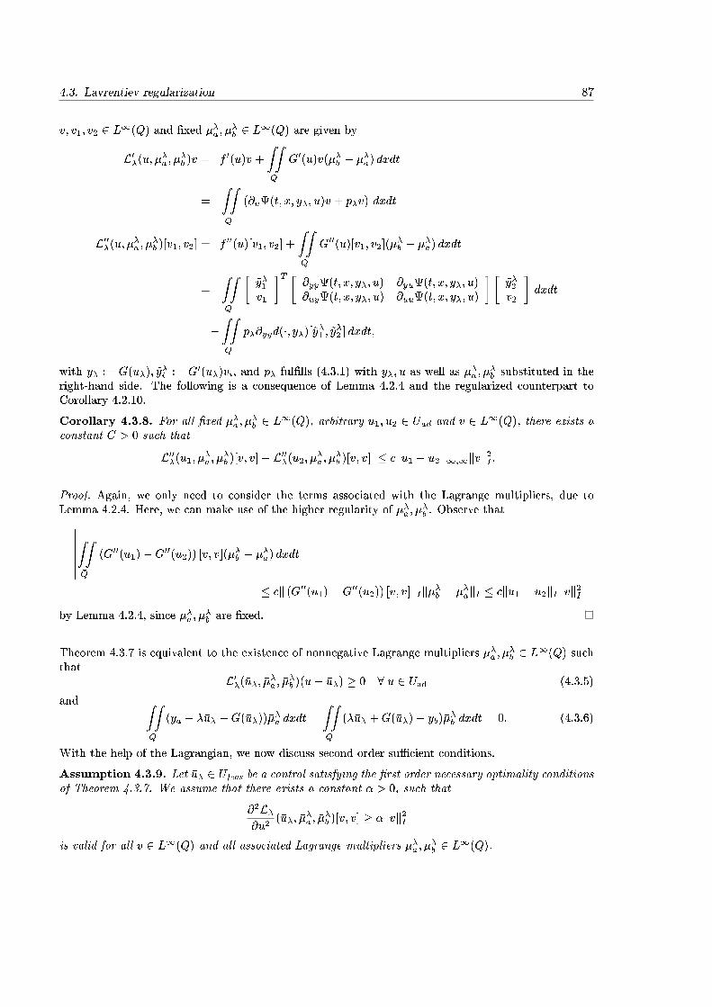
4.3. Lavrentiev regularization 87
v; v1; v2 2 L1(Q) and �xed ��a ; ��b 2 L1(Q) are given by
L0�(u; ��a ; ��b )v = f 0(u)v +
ZZQ
G0(u)v(��b � ��a) dxdt
=
ZZ�Q
(@u(t; x; y�; u)v + p�v) dxdt
L00�(u; ��a ; ��b )[v1; v2] = f 00(u)[v1; v2] +
ZZQ
G00(u)[v1; v2](��b � ��a) dxdt
=
ZZQ
�~y�1v1
�T �@yy(t; x; y�; u) @yu(t; x; y�; u)@uy(t; x; y�; u) @uu(t; x; y�; u)
� �~y�2v2
�dxdt
�ZZQ
p�@yyd(�; y�)[~y�1 ; ~y�2 ] dxdt;
with y� := G(u�); ~y�i := G0(u�)vi, and p� ful�lls (4.3.1) with y�; u as well as ��a ; �
�b substituted in the
right-hand side. The following is a consequence of Lemma 4.2.4 and the regularized counterpart toCorollary 4.2.10.
Corollary 4.3.8. For all �xed ��a ; ��b 2 L1(Q), arbitrary u1; u2 2 Uad and v 2 L1(Q), there exists a
constant C > 0 such that
jL00�(u1; ��a ; ��b )[v; v]� L00�(u2; ��a ; ��b )[v; v]j � cku1 � u2k1;1kvk2I :
Proof. Again, we only need to consider the terms associated with the Lagrange multipliers, due toLemma 4.2.4. Here, we can make use of the higher regularity of ��a ; �
�b . Observe that�������
ZZ�Q
(G00(u1)�G00(u2)) [v; v](��b � ��a) dxdt
�������� ck (G00(u1)�G00(u2)) [v; v]kIk��b � ��akI � cku1 � u2kIkvk2I
by Lemma 4.2.4, since ��a ; ��b are �xed.
Theorem 4.3.7 is equivalent to the existence of nonnegative Lagrange multipliers ���a ; ���b 2 L1(Q) such
thatL0�(�u�; ���a ; ���b )(u� �u�) � 0 8 u 2 Uad (4.3.5)
and ZZQ
(ya � ��u� �G(�u�))���a dxdt =
ZZQ
(��u� +G(�u�)� yb)���b dxdt = 0: (4.3.6)
With the help of the Lagrangian, we now discuss second order su�cient conditions.
Assumption 4.3.9. Let �u� 2 Ufeas be a control satisfying the �rst order necessary optimality conditionsof Theorem 4.3.7. We assume that there exists a constant � > 0, such that
@2L�@u2
(�u�; ���a ; ��
�b )[v; v] � �kvk2I
is valid for all v 2 L1(Q) and all associated Lagrange multipliers ���a ; ���b 2 L1(Q).
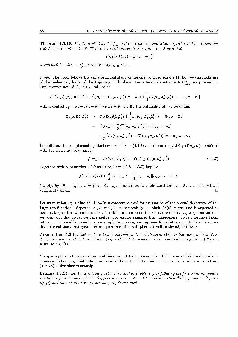
88 4. A parabolic control problem with pointwise state and control constraints
Theorem 4.3.10. Let the control �u� 2 U�feas and the Lagrange multipliers ���a ; ���b ful�ll the conditions
stated in Assumption 4.3.9. Then there exist constants � > 0 and " > 0 such that
f(u) � f(�u�) + �ku� �u�k2Iis satis�ed for all u 2 U�feas with ku� �u�k1;1 � ".
Proof. The proof follows the same principal steps as the one for Theorem 4.2.11, but we can make useof the higher regularity of the Lagrange multipliers. For a feasible control u 2 U�feas, we proceed byTaylor expansion of L� in �u� and obtain
L�(u; ���a ; ���b ) = L�(�u�; ���a ; ���b ) + L0�(�u�; ���a)(u� �u�) +1
2L00�(u�; ���a ; ���b )[u� �u�; u� �u�]
with a control u� = �u� + �(u� �u�) with � 2 (0; 1). By the optimality of �u�, we obtain
L�(u; ���a ; ���b ) � L�(�u�; ���a ; ���b ) +1
2L00�(u�; ���a ; ���b )[u� �u�; u� �u�]
= L�(�u�) + 1
2L00�(�u�; ���a ; ���b )[u� �u�; u� �u�]
+1
2
�L00�(u�; ���a ; ���b )� L00�(�u�; ���a ; ���b )� [u� �u�; u� �u�]:
In addition, the complementary slackness conditions (4.3.3) and the nonnegativity of ���a ; ���b combined
with the feasibility of u, imply
f(�u�) = L�(�u�; ���a ; ���b ); f(u) � L�(u; ���a ; ���b ): (4.3.7)
Together with Assumption 4.3.9 and Corollary 4.3.8, (4.3.7) implies
f(u) � f(�u�) +�
2ku� �u�k2 � c
2k�u� � u�k1;1ku� �u�k2I :
Clearly, by k�u� � u�k1;1 = �ku � �u�k1;1, the assertion is obtained for ku � �u�k1;1 � " with "su�ciently small.
Let us mention again that the Lipschitz constant c used for estimation of the second derivative of theLagrange functional depends on ���a and ���b , more precisely: on their L2(Q) norm, and is expected tobecome large when � tends to zero. To elaborate more on the structure of the Lagrange multipliers,we point out that so far we have neither proven nor assumed their uniqueness. So far, we have takeninto account possible nonuniqueness simply by making assumptions for arbitrary multipliers. Now, wediscuss conditions that guarantee uniqueness of the multipliers as well as the adjoint state.
Assumption 4.3.11. Let �u� be a locally optimal control of Problem (P�) in the sense of De�nition4.3.3. We assume that there exists � > 0 such that the �-active sets according to De�nition 4.3.4 arepairwise disjoint.
Comparing this to the separation conditions formulated in Assumption 4.3.5 we now additionally excludesituations where e.g. both the lower control bound and the lower mixed control-state constraint are(almost) active simultaneously.
Lemma 4.3.12. Let �u� be a locally optimal control of Problem (P�) ful�lling the �rst order optimalityconditions from Theorem 4.3.7. Suppose that Assumption 4.3.11 holds. Then the Lagrange multipliers���a ; ��
�b and the adjoint state �p� are uniquely determined.
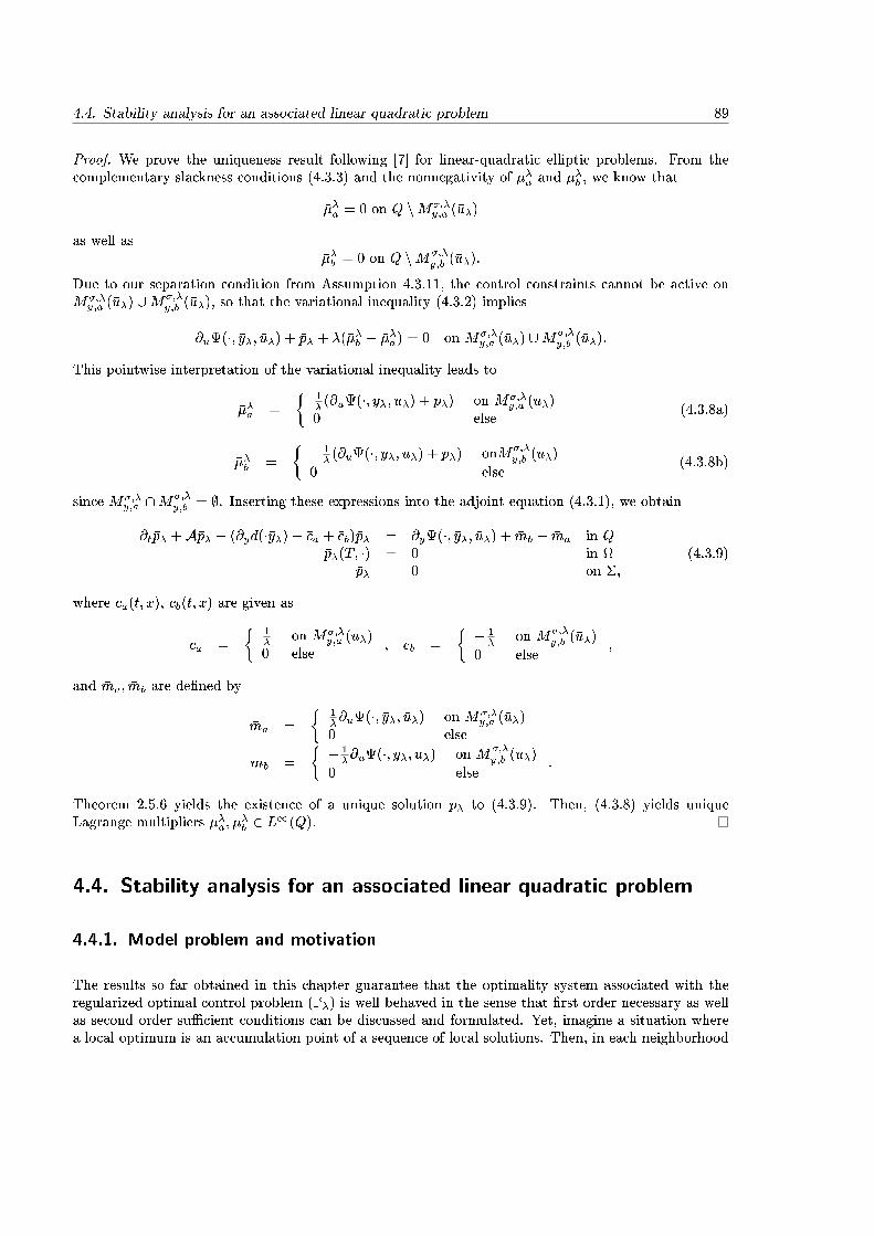
4.4. Stability analysis for an associated linear quadratic problem 89
Proof. We prove the uniqueness result following [7] for linear-quadratic elliptic problems. From thecomplementary slackness conditions (4.3.3) and the nonnegativity of ���a and ���b , we know that
���a = 0 on Q nM�;�y;a (�u�)
as well as���b = 0 on Q nM�;�
y;b (�u�):
Due to our separation condition from Assumption 4.3.11, the control constraints cannot be active onM�;�y;a (�u�) [M�;�
y;b (�u�), so that the variational inequality (4.3.2) implies
@u(�; �y�; �u�) + �p� + �(���b � ���a) = 0 on M�;�y;a (�u�) [M�;�
y;b (�u�):
This pointwise interpretation of the variational inequality leads to
���a =
�1� (@u(�; �y�; �u�) + �p�) on M�;�
y;a (�u�)0 else
(4.3.8a)
���b =
� � 1� (@u(�; �y�; �u�) + �p�) onM�;�
y;b (�u�)
0 else(4.3.8b)
since M�;�y;a \M�;�
y;b = ;. Inserting these expressions into the adjoint equation (4.3.1), we obtain
@t�p� +A�p� + (@yd(��y�) + �ca + �cb)�p� = @y(�; �y�; �u�) + �mb � �ma in Q�p�(T; �) = 0 in
�p� = 0 on �;(4.3.9)
where �ca(t; x); �cb(t; x) are given as
�ca =
�1� on M�;�
y;a (�u�)0 else
; �cb =
� � 1� on M�;�
y;b (�u�)
0 else;
and �ma; �mb are de�ned by
�ma =
�1�@u(�; �y�; �u�) on M�;�
y;a (�u�)0 else
�mb =
� � 1�@u(�; �y�; �u�) on M�;�
y;b (�u�)
0 else:
Theorem 2.5.6 yields the existence of a unique solution �p� to (4.3.9). Then, (4.3.8) yields uniqueLagrange multipliers ���a ; ��
�b 2 L1(Q).
4.4. Stability analysis for an associated linear quadratic problem
4.4.1. Model problem and motivation
The results so far obtained in this chapter guarantee that the optimality system associated with theregularized optimal control problem (P�) is well behaved in the sense that �rst order necessary as wellas second order su�cient conditions can be discussed and formulated. Yet, imagine a situation wherea local optimum is an accumulation point of a sequence of local solutions. Then, in each neighborhood
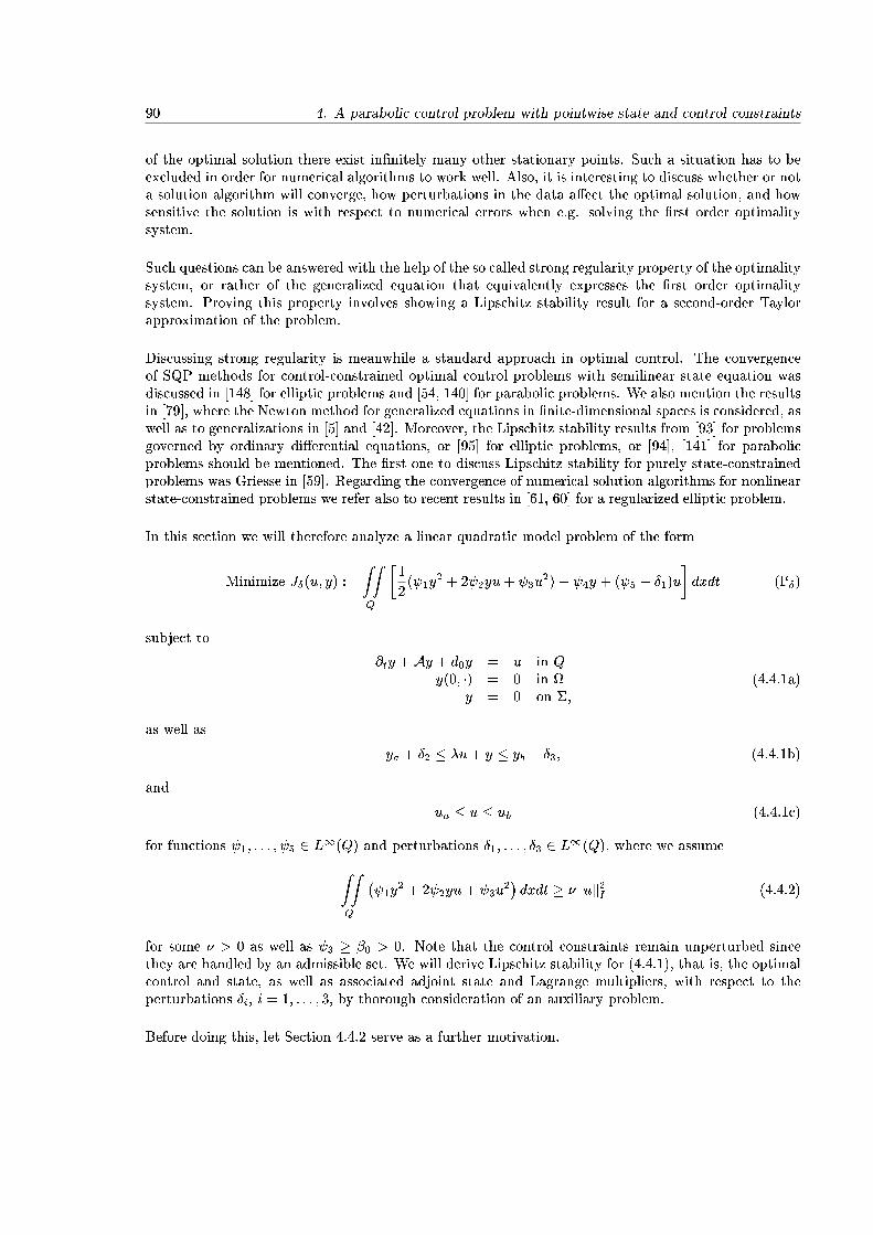
90 4. A parabolic control problem with pointwise state and control constraints
of the optimal solution there exist in�nitely many other stationary points. Such a situation has to beexcluded in order for numerical algorithms to work well. Also, it is interesting to discuss whether or nota solution algorithm will converge, how perturbations in the data a�ect the optimal solution, and howsensitive the solution is with respect to numerical errors when e.g. solving the �rst order optimalitysystem.
Such questions can be answered with the help of the so called strong regularity property of the optimalitysystem, or rather of the generalized equation that equivalently expresses the �rst order optimalitysystem. Proving this property involves showing a Lipschitz stability result for a second-order Taylorapproximation of the problem.
Discussing strong regularity is meanwhile a standard approach in optimal control. The convergenceof SQP methods for control-constrained optimal control problems with semilinear state equation wasdiscussed in [148] for elliptic problems and [54, 140] for parabolic problems. We also mention the resultsin [79], where the Newton method for generalized equations in �nite-dimensional spaces is considered, aswell as to generalizations in [5] and [42]. Moreover, the Lipschitz stability results from [93] for problemsgoverned by ordinary di�erential equations, or [95] for elliptic problems, or [94], [141] for parabolicproblems should be mentioned. The �rst one to discuss Lipschitz stability for purely state-constrainedproblems was Griesse in [59]. Regarding the convergence of numerical solution algorithms for nonlinearstate-constrained problems we refer also to recent results in [61, 60] for a regularized elliptic problem.
In this section we will therefore analyze a linear quadratic model problem of the form
Minimize J�(u; y) :=
ZZQ
�1
2( 1y
2 + 2 2yu+ 3u2) + 4y + ( 5 � �1)u
�dxdt (P�)
subject to
@ty +Ay + d0y = u in Qy(0; �) = 0 in
y = 0 on �;(4.4.1a)
as well as
ya + �2 � �u+ y � yb � �3; (4.4.1b)
and
ua � u � ub (4.4.1c)
for functions 1; : : : ; 5 2 L1(Q) and perturbations �1; : : : ; �3 2 L1(Q), where we assumeZZQ
� 1y
2 + 2 2yu+ 3u2�dxdt � �kuk2I (4.4.2)
for some � > 0 as well as 3 � �0 > 0. Note that the control constraints remain unperturbed sincethey are handled by an admissible set. We will derive Lipschitz stability for (4.4.1), that is, the optimalcontrol and state, as well as associated adjoint state and Lagrange multipliers, with respect to theperturbations �i, i = 1; : : : ; 3, by thorough consideration of an auxiliary problem.
Before doing this, let Section 4.4.2 serve as a further motivation.
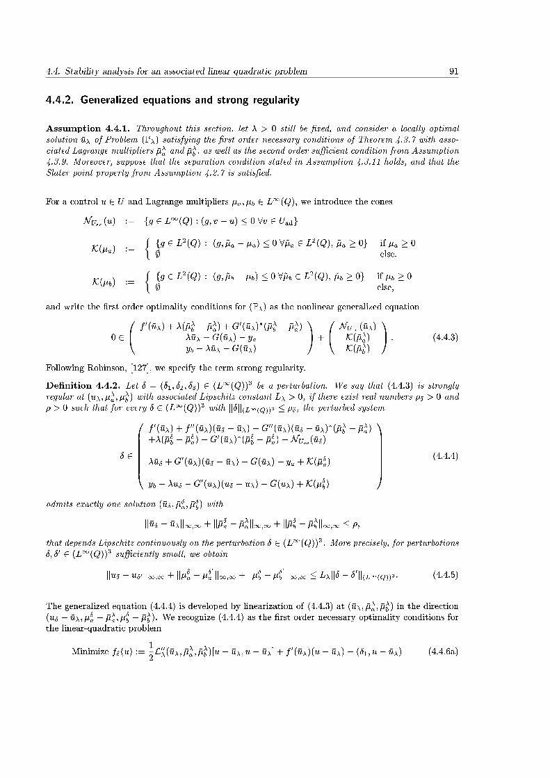
4.4. Stability analysis for an associated linear quadratic problem 91
4.4.2. Generalized equations and strong regularity
Assumption 4.4.1. Throughout this section, let � > 0 still be �xed, and consider a locally optimalsolution �u� of Problem (P�) satisfying the �rst order necessary conditions of Theorem 4.3.7 with asso-ciated Lagrange multipliers ���a and ���b , as well as the second order su�cient condition from Assumption4.3.9. Moreover, suppose that the separation condition stated in Assumption 4.3.11 holds, and that theSlater point property from Assumption 4.2.7 is satis�ed.
For a control u 2 U and Lagrange multipliers �a; �b 2 L1(Q), we introduce the cones
NUad(u) := fg 2 L1(Q) : (g; v � u) � 0 8v 2 Uadg
K(�a) :=
� fg 2 L2(Q) : (g; ~�a � �a) � 0 8~�a 2 L2(Q); ~�a � 0g if �a � 0; else:
K(�b) :=
� fg 2 L2(Q) : (g; ~�b � �b) � 0 8~�b 2 L2(Q); ~�b � 0g if �b � 0; else;
and write the �rst order optimality conditions for (P�) as the nonlinear generalized equation
0 20@ f 0(�u�) + �(���b � ���a) +G0(�u�)
�(���b � ���a)��u� +G(�u�)� yayb � ��u� �G(�u�)
1A+
0@ NUad(�u�)K(���a)K(���b )
1A : (4.4.3)
Following Robinson, [127], we specify the term strong regularity.
De�nition 4.4.2. Let � = (�1; �2; �3) 2 (L1(Q))3 be a perturbation. We say that (4.4.3) is stronglyregular at (�u�; ��
�a ; ��
�b ) with associated Lipschitz constant L� > 0, if there exist real numbers �� > 0 and
� > 0 such that for every � 2 (L1(Q))3 with k�k(L1(Q))3 � ��, the perturbed system
� 2
0BBBBBB@f 0(�u�) + f 00(�u�)(�u� � �u�) +G00(�u�)(�u� � �u�)
�(���b � ���a)+�(���b � ���a) +G0(�u�)
�(���b � ���a) +NUad(�u�)
��u� +G0(�u�)(�u� � �u�) +G(�u�)� ya +K(���a)
yb � ��u� �G0(�u�)(�u� � �u�)�G(�u�) +K(���b)
1CCCCCCA (4.4.4)
admits exactly one solution (�u�; ���a; ��
�b) with
k�u� � �u�k1;1 + k���a � ���ak1;1 + k���b � ���b k1;1 � �;
that depends Lipschitz continuously on the perturbation � 2 (L1(Q))3. More precisely, for perturbations�; �0 2 (L1(Q))3 su�ciently small, we obtain
k�u� � �u�0k1;1 + k���a � ���0
a k1;1 + k���b � ���0
b k1;1 � L�k� � �0k(L1(Q))3 : (4.4.5)
The generalized equation (4.4.4) is developed by linearization of (4.4.3) at (�u�; ���a ; ��
�b ) in the direction
(u� � �u�; ��a � ���a ; �
�b � ���b ). We recognize (4.4.4) as the �rst order necessary optimality conditions for
the linear-quadratic problem
Minimize f�(u) :=1
2L00�(�u�; ���a ; ���b )[u� �u�; u� �u�] + f 0(�u�)(u� �u�)� (�1; u� �u�) (4.4.6a)

92 4. A parabolic control problem with pointwise state and control constraints
subject to
ya + �2 � ��u� �G(�u�) � �(u� �u�) +G0(�u�)(u� �u�) � yb � �3 � ��u� �G(�u�); (4.4.6b)
as well asua � u � ub (4.4.6c)
with optimal control �u� and associated Lagrange multipliers ���a; ���b , if these exist in regular spaces. To
obtain strong regularity of the generalized equation (4.4.3) we will therefore have to
1. prove existence of a unique optimal control �u� of Problem (4.4.6)
2. show the existence of an associated Slater point and obtain the existence of (irregular) Lagrangemultipliers
3. prove a separation condition in the spirit of Assumption 3.4.2 to obtain higher regularity anduniqueness of the Lagrange multipliers
4. obtain the desired Lipschitz property (4.4.5)
for su�ciently small � 2 L1(Q)3. Steps 1) and 2) are easily shown:
Lemma 4.4.3. Let Assumption 4.4.1 hold. Then the linear-quadratic optimal control problem (4.4.6)admits a unique optimal control �u�. Moroever, for �2; �3 small enough, the Slater point u� from As-sumption 4.2.7 is also a Slater point for Problem (4.4.6)
Proof. First observe that the feasible set for Problem (4.4.6) is not empty, since �u� satis�es all con-straints. The existence of a unique solution to this problem can then be deduced from the second ordersu�cient condition for �u� stated in Assumption (4.3.9). More precisely, Assumption (4.3.9) guaran-tees that the objective function f� is strictly convex for every � 2 (L1(Q))3 and tends to in�nity askukI !1, which yields the existence of a unique solution by standard arguments. Moreover, the upperstate constraint can be rewritten as
�u+G(�u�) +G0(�u�)(u� �u�)� yb + �3 � 0:
To check the Slater point property, note that the derivatives have to be taken with respect to u, andwe obtain
��u� +G(�u�)� yb + �3 +G0(�u�)(�u� � �u�) + �(u� � �u�) +G0(�u�)(u� � �u�)
= �u� +G(�u�) +G0(�u�)(u� � �u�)� yb + �3
� �=2
for �3 su�ciently small. The lower state constraint and the control constraints are treated analogously.Consequently, there exist Lagrange multipliers ���a; ��
�b 2 L1(Q)�, cf. the discussion in [134].
Steps 3) and 4) will be the heart of the proof of strong regularity. For �1 = �2 = �3 = 0, the separationcondition and therefore uniqueness and higher regularity of the multipliers is easily obtained notingthat �u� with associated Lagrange multipliers solves the linearized unperturbed problem, since the �rstinclusion in (4.4.4) simpli�es to
0 2 f 0(�u�) + �(���b � ���a) +G0(�u�)�(���b � ���a) +NUad(�u�):
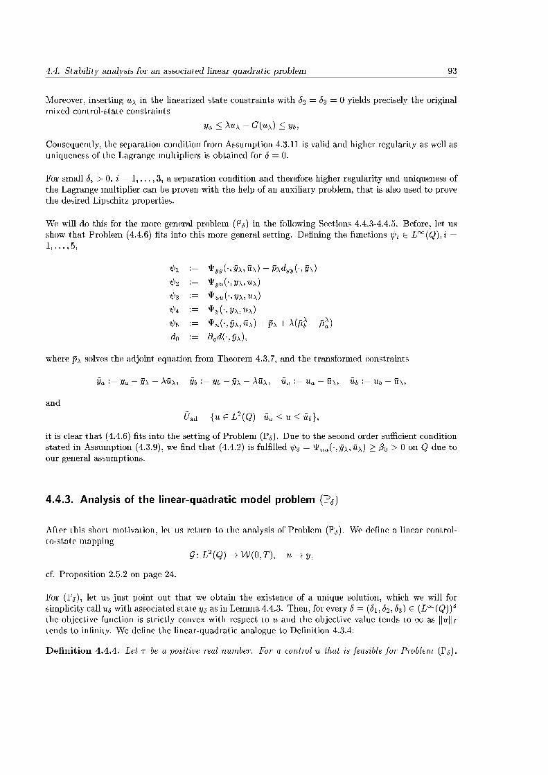
4.4. Stability analysis for an associated linear quadratic problem 93
Moreover, inserting �u� in the linearized state constraints with �2 = �3 = 0 yields precisely the originalmixed control-state constraints
ya � ��u� +G(�u�) � yb;
Consequently, the separation condition from Assumption 4.3.11 is valid and higher regularity as well asuniqueness of the Lagrange multipliers is obtained for � = 0.
For small �i > 0, i = 1; : : : ; 3, a separation condition and therefore higher regularity and uniqueness ofthe Lagrange multiplier can be proven with the help of an auxiliary problem, that is also used to provethe desired Lipschitz properties.
We will do this for the more general problem (P�) in the following Sections 4.4.3-4.4.5. Before, let usshow that Problem (4.4.6) �ts into this more general setting. De�ning the functions i 2 L1(Q); i =1; : : : ; 5,
1 := yy(�; �y�; �u�)� �p�dyy(�; �y�) 2 := yu(�; �y�; �u�) 3 := uu(�; �y�; �u�) 4 := y(�; �y�; �u�) 5 := u(�; �y�; �u�) + �p� + �(���b � ���a)
d0 := @yd(�; �y�);
where �p� solves the adjoint equation from Theorem 4.3.7, and the transformed constraints
~ya := ya � �y� � ��u�; ~yb := yb � �y� � ��u�; ~ua := ua � �u�; ~ub := ub � �u�;
and
~Uad = fu 2 L2(Q) j ~ua � u � ~ubg;it is clear that (4.4.6) �ts into the setting of Problem (P�). Due to the second order su�cient conditionstated in Assumption (4.3.9), we �nd that (4.4.2) is ful�lled 3 = uu(�; �y�; �u�) � �0 > 0 on Q due toour general assumptions.
4.4.3. Analysis of the linear-quadratic model problem (P�)
After this short motivation, let us return to the analysis of Problem (P�). We de�ne a linear control-to-state mapping
G : L2(Q)!W(0; T ); u 7! y;
cf. Proposition 2.5.2 on page 24.
For (P�), let us just point out that we obtain the existence of a unique solution, which we will forsimplicity call �u� with associated state �y� as in Lemma 4.4.3. Then, for every � = (�1; �2; �3) 2 (L1(Q))3
the objective function is strictly convex with respect to u and the objective value tends to 1 as kukItends to in�nity. We de�ne the linear-quadratic analogue to De�nition 4.3.4:
De�nition 4.4.4. Let � be a positive real number. For a control u that is feasible for Problem (P�),
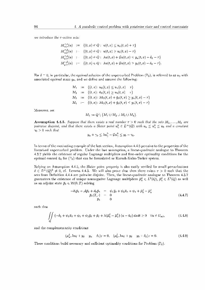
94 4. A parabolic control problem with pointwise state and control constraints
we introduce the � -active sets:
M�;�u;a(u) := f(t; x) 2 Q : u(t; x) � ua(t; x) + �g
M�;�u;b (u) := f(t; x) 2 Q : u(t; x) � ub(t; x)� �g
M�;�y;a(u) := f(t; x) 2 Q : �u(t; x) + Gu(t; x) � ya(t; x) + �2 + �g
M�;�y;b (u) := f(t; x) 2 Q : �u(t; x) + Gu(t; x) � yb(t; x)� �3 � �g:
For � � 0, in particular, the optimal solution of the unperturbed Problem (P0), is referred to as �u0 withassociated optimal state �y0, and we de�ne and assume the following:
M1 := f(t; x) : �u0(t; x) � ua(t; x) + �gM2 := f(t; x) : �u0(t; x) � ub(t; x)� �gM3 := f(t; x) : ��u0(t; x) + �y0(t; x) � ya(t; x) + �gM4 := f(t; x) : ��u0(t; x) + �y0(t; x) � yb(t; x)� �g
Moreover, set
M5 := Q n fM1 [M2 [M3 [M4g:Assumption 4.4.5. Suppose that there exists a real number � > 0 such that the sets M1; : : : ;M5 arepairwise disjoint, and that there exists a Slater point u0 2 L1(Q) with ua � u0 � ub and a constant 0 > 0 such that
ya + 0 � �u0 + Gu0 � yb � 0:
In terms of the motivating example of the last section, Assumption 4.4.5 pertains to the properties of thelinearized unperturbed problem. Under the last assumption, a linear-quadratic analogue to Theorem4.3.7 yields the existence of regular Lagrange multipliers and �rst-order optimality conditions for theoptimal control �u0 for (P0) that can be formulated as Karush-Kuhn-Tucker system.
Relying on Assumption 4.4.5, the Slater point property is also easily veri�ed for small perturbations� 2 L1(Q)3 6= 0, cf. Lemma 4.4.3. We will also prove that then there exists � > 0 such that thesets from De�nition 4.4.4 are pairwise disjoint. Then, the linear-quadratic analogue to Theorem 4.3.7guarantees the existence of unique nonnegative Lagrange multipliers ���a 2 L2(Q); ���b 2 L2(Q) as wellas an adjoint state �p� 2 W(0; T ) solving
�@t�p� +A�p� + d0�p� = 1�y� + 2�u� + 4 + ���b � ���a�p�(T; �) = 0
�p� = 0(4.4.7)
such thatZZQ
���1 + 3�u� + 5 + 2�y� + �p� + �(���b � ���a�(u� �u�) dxdt � 0 8u 2 Uad; (4.4.8)
and the complementarity conditions
(���a; ��u� + �y� � ya � �2)I = 0; (���b ; ��u� + �y� � yb + �3)I = 0: (4.4.9)
These conditions build necessary and su�cient optimality conditions for Problem (P�).
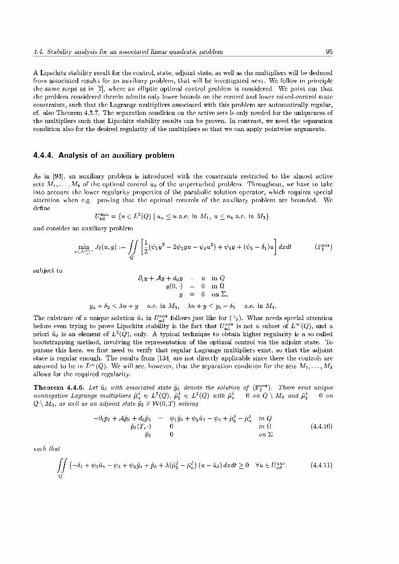
4.4. Stability analysis for an associated linear quadratic problem 95
A Lipschitz stability result for the control, state, adjoint state, as well as the multipliers will be deducedfrom associated results for an auxiliary problem, that will be investigated next. We follow in principlethe same steps as in [7], where an elliptic optimal control problem is considered. We point out thatthe problem considered therein admits only lower bounds on the control and lower mixed-control stateconstraints, such that the Lagrange multipliers associated with this problem are automatically regular,cf. also Theorem 4.3.7. The separation condition on the active sets is only needed for the uniqueness ofthe multipliers such that Lipschitz stability results can be proven. In contrast, we need the separationcondition also for the desired regularity of the multipliers so that we can apply pointwise arguments.
4.4.4. Analysis of an auxiliary problem
As in [93], an auxiliary problem is introduced with the constraints restricted to the almost activesets M1; : : : ;M4 of the optimal control �u0 of the unperturbed problem. Throughout, we have to takeinto account the lower regularity properties of the parabolic solution operator, which requires specialattention when e.g. proving that the optimal controls of the auxiliary problem are bounded. Wede�ne
Uauxad = fu 2 L2(Q) j ua � u a.e. in M1; u � ub a.e. in M2g;
and consider an auxiliary problem
minu2Uaux
ad
J�(u; y) :=
ZZQ
�1
2( 1y
2 + 2 2yu+ 3u2) + 4y + ( 5 � �1)u
�dxdt (Paux� )
subject to@ty +Ay + d0y = u in Q
y(0; �) = 0 in y = 0 on �;
ya + �2 � �u+ y a.e. in M3; �u+ y � yb � �3 a.e. in M4:
The existence of a unique solution ~u� in Uauxad follows just like for (P�). What needs special attention
before even trying to prove Lipschitz stability is the fact that Uauxad is not a subset of L1(Q), and a
priori ~u� is an element of L2(Q), only. A typical technique to obtain higher regularity is a so-calledbootstrapping method, involving the representation of the optimal control via the adjoint state. Topursue this here, we �rst need to verify that regular Lagrange multipliers exist, so that the adjointstate is regular enough. The results from [134] are not directly applicable since there the controls areassumed to be in L1(Q). We will see, however, that the separation condition for the sets M1; : : : ;M4
allows for the required regularity.
Theorem 4.4.6. Let ~u� with associated state ~y� denote the solution of (Paux� ). There exist uniquenonnegative Lagrange multipliers ~��a 2 L2(Q); ~��b 2 L2(Q) with ~��a = 0 on Q nM3 and ~��b = 0 onQ nM4, as well as an adjoint state ~p� 2 W(0; T ) solving
�@t~p� +A~p� + d0~p� = 1~y� + 2~u� + 4 + ~��b � ~��a in Q~p�(T; �) = 0 in
~p� = 0 on �(4.4.10)
such thatZZQ
���1 + 3~u� + 5 + 2~y� + ~p� + �(~��b � ~��a�(u� ~u�) dxdt � 0 8u 2 Uaux
ad ; (4.4.11)

96 4. A parabolic control problem with pointwise state and control constraints
and the complementarity conditions
(~��a; �~u� + ~y� � ya � �2)I = 0; (~��b ; �~u� + ~y� � yb + �3)I = 0 (4.4.12)
are satis�ed. The Lagrange multipliers associated with the solution of (Paux� ) admit the form
~��a = maxf0; 3�2
(ya + �2 � ~y�) +1
3(��1 + 5 + 2~y� + ~p�)g on M3 (4.4.13)
~��b = maxf0; 3�2
(~y� + �3 � yb)� 1
3(��1 + 5 + 2~y� + ~p�)g on M4: (4.4.14)
Proof. Let us �rst express the constraints of (Paux� )
�u � �ua on M1; ��u� Gu � �ya � �2 on M3;u � ub on M2; �u+ Gu � yb � �3 on M4;
u(t; x) 2 R on M(4.4.15)
in another form. De�ne the linear operator
G : L2(Q)! L2(Q); Gu = (�2 � �1 + �5)u+ (�4 � �3)(�u+ Gu);
where the �i, i = 1; : : : ; 5 are the characteristic functions of the sets Mi. Then (4.4.15) is equivalent to
(Gu)(t; x)
� � b(t; x) on Q nM5
arbitrary on M5;
whereb(t; x) = ��1ua + �2ub � �3(�ya � �2) + �4(yb � �3):
We now show that this system satis�es the well-known regularity condition by Zowe and Kurcyusz,[153]. To introduce it, we need the convex cone
K(�v) = f�(v � �v) j � � 0; v � 0 on Q nM5; v 2 L2(Q)g:
Notice that v is arbitrary on M5, since no constraints are given there. There is no further constraintimposed on u, hence the Zowe-Kurcyusz-regularity condition is
G(L2(Q)) +K(�G~u�) = L2(Q);
i.e. each z 2 L2(Q) can be represented in the form
z = Gu+ �(v +G~u�);
with v � 0 on Q nM5, u 2 L2(Q), � � 0. It turns out that � = 0 can be taken and also v = 0, i.e.Gu = z. A comparison with (4.4.15) shows that we can take
u =
� �z on M1
z on M2 [M5:(4.4.16)
It remains to �nd u on M3 [M4. De�ne u as the function that satis�es (4.4.16) on M1 [M2 [M5 andis zero on M3 [M4. Then, we can decompose u into
u = u3 + u4 + u;
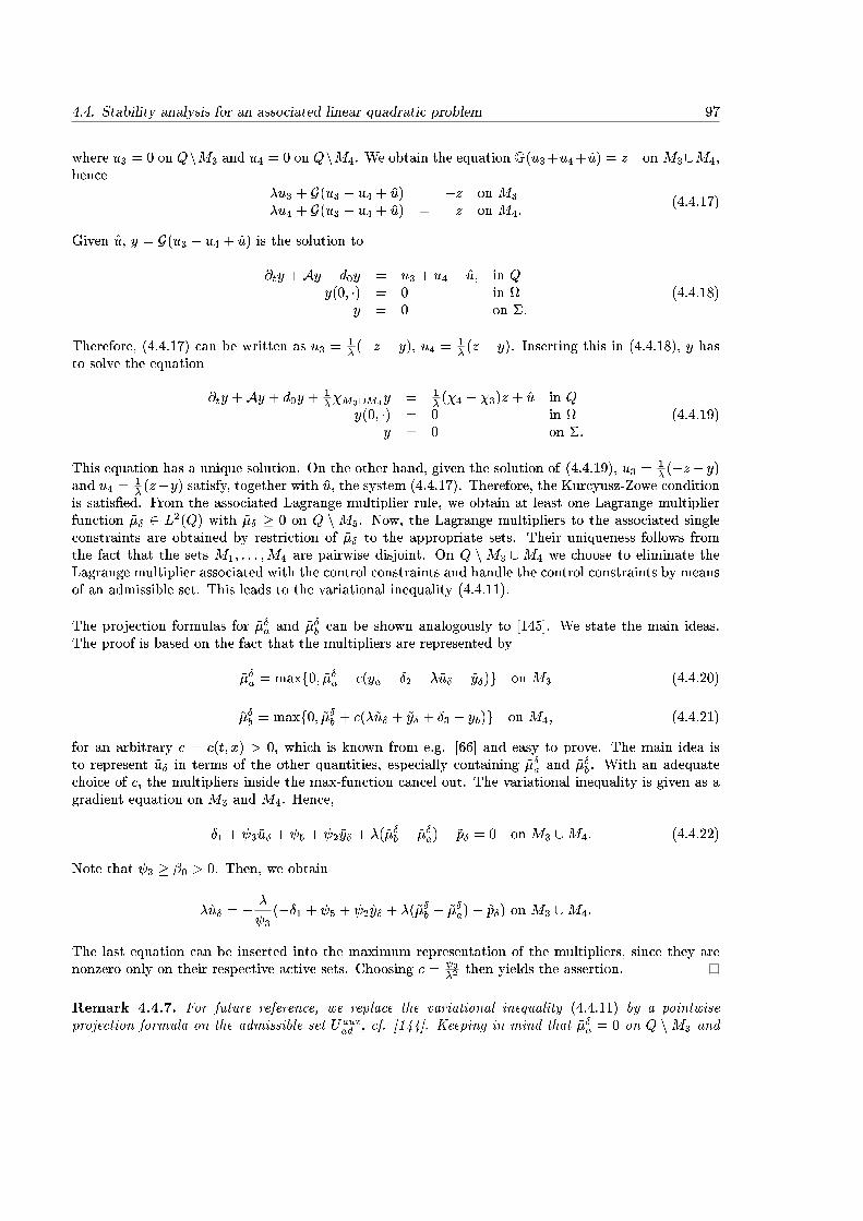
4.4. Stability analysis for an associated linear quadratic problem 97
where u3 = 0 on QnM3 and u4 = 0 on QnM4. We obtain the equation G(u3+u4+u) = z on M3[M4;hence
�u3 + G(u3 + u4 + u) = �z on M3
�u4 + G(u3 + u4 + u) = z on M4:(4.4.17)
Given u, y = G(u3 + u4 + u) is the solution to
@ty +Ay + d0y = u3 + u4 + u; in Qy(0; �) = 0 in
y = 0 on �:(4.4.18)
Therefore, (4.4.17) can be written as u3 =1� (�z � y), u4 =
1� (z � y). Inserting this in (4.4.18), y has
to solve the equation
@ty +Ay + d0y +1��M3[M4
y = 1� (�4 � �3)z + u in Q
y(0; �) = 0 in y = 0 on �:
(4.4.19)
This equation has a unique solution. On the other hand, given the solution of (4.4.19), u3 =1� (�z� y)
and u4 =1� (z�y) satisfy, together with u, the system (4.4.17). Therefore, the Kurcyusz-Zowe condition
is satis�ed. From the associated Lagrange multiplier rule, we obtain at least one Lagrange multiplierfunction ~�� 2 L2(Q) with ~�� � 0 on Q nM5. Now, the Lagrange multipliers to the associated singleconstraints are obtained by restriction of ~�� to the appropriate sets. Their uniqueness follows fromthe fact that the sets M1; : : : ;M4 are pairwise disjoint. On Q nM3 [M4 we choose to eliminate theLagrange multiplier associated with the control constraints and handle the control constraints by meansof an admissible set. This leads to the variational inequality (4.4.11).
The projection formulas for ~��a and ~��b can be shown analogously to [145]. We state the main ideas.The proof is based on the fact that the multipliers are represented by
~��a = maxf0; ~��a + c(ya + �2 � �~u� � ~y�)g on M3 (4.4.20)
~��b = maxf0; ~��b + c(�~u� + ~y� + �3 � yb)g on M4; (4.4.21)
for an arbitrary c = c(t; x) > 0, which is known from e.g. [66] and easy to prove. The main idea isto represent ~u� in terms of the other quantities, especially containing ~��a and ~��b . With an adequatechoice of c, the multipliers inside the max-function cancel out. The variational inequality is given as agradient equation on M3 and M4. Hence,
��1 + 3~u� + 5 + 2~y� + �(~��b � ~��a) + ~p� = 0 on M3 [M4: (4.4.22)
Note that 3 � �0 > 0. Then, we obtain
�~u� = � �
3(��1 + 5 + 2~y� + �(~��b � ~��a) + ~p�) on M3 [M4:
The last equation can be inserted into the maximum representation of the multipliers, since they arenonzero only on their respective active sets. Choosing c = 3
�2 then yields the assertion.
Remark 4.4.7. For future reference, we replace the variational inequality (4.4.11) by a pointwiseprojection formula on the admissible set Uaux
ad , cf. [144]. Keeping in mind that ~��a = 0 on Q nM3 and
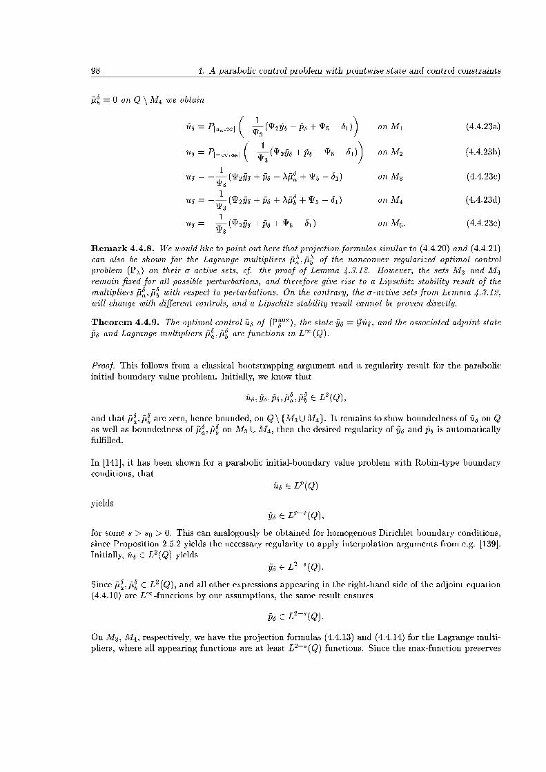
98 4. A parabolic control problem with pointwise state and control constraints
~��b = 0 on Q nM4 we obtain
~u� = P[ua;1]
�� 1
3(2~y� + ~p� +5 � �1)
�on M1 (4.4.23a)
u� = P[�1;ub]
�� 1
3(2~y� + ~p� +5 � �1)
�on M2 (4.4.23b)
u� = � 1
3(2~y� + ~p� � �~��a +5 � �1) on M3 (4.4.23c)
u� = � 1
3(2~y� + ~p� + �~��b +5 � �1) on M4 (4.4.23d)
u� = � 1
3(2~y� + ~p� +5 � �1) on M5: (4.4.23e)
Remark 4.4.8. We would like to point out here that projection formulas similar to (4.4.20) and (4.4.21)can also be shown for the Lagrange multipliers ���a ; ��
�b of the nonconvex regularized optimal control
problem (P�) on their �-active sets, cf. the proof of Lemma 4.3.12. However, the sets M3 and M4
remain �xed for all possible perturbations, and therefore give rise to a Lipschitz stability result of themultipliers ~��a; ~�
�b with respect to perturbations. On the contrary, the �-active sets from Lemma 4.3.12,
will change with di�erent controls, and a Lipschitz stability result cannot be proven directly.
Theorem 4.4.9. The optimal control ~u� of (Paux� ), the state ~y� = G~u�, and the associated adjoint state
~p� and Lagrange multipliers ~��a; ~��b are functions in L
1(Q).
Proof. This follows from a classical bootstrapping argument and a regularity result for the parabolicinitial boundary value problem. Initially, we know that
~u�; ~y�; ~p�; ~��a; ~�
�b 2 L2(Q);
and that ~��a; ~��b are zero, hence bounded, on QnfM3[M4g. It remains to show boundedness of ~u� on Q
as well as boundedness of ~��a; ~��b on M3 [M4, then the desired regularity of ~y� and ~p� is automatically
ful�lled.
In [141], it has been shown for a parabolic initial-boundary value problem with Robin-type boundaryconditions, that
~u� 2 Lp(Q)yields
~y� 2 Lp+s(Q);for some s > s0 > 0. This can analogously be obtained for homogenous Dirichlet boundary conditions,since Proposition 2.5.2 yields the necessary regularity to apply interpolation arguments from e.g. [139].Initially, ~u� 2 L2(Q) yields
~y� 2 L2+s(Q):
Since ~��a; ~��b 2 L2(Q), and all other expressions appearing in the right-hand side of the adjoint equation
(4.4.10) are L1-functions by our assumptions, the same result ensures
~p� 2 L2+s(Q):
On M3, M4, respectively, we have the projection formulas (4.4.13) and (4.4.14) for the Lagrange multi-pliers, where all appearing functions are at least L2+s(Q) functions. Since the max-function preserves
4.4. Stability analysis for an associated linear quadratic problem 99
this regularity, we obtain L2+s-regularity of ~��a on M3 and ~��b on M4. Recalling that the multipliers arezero outside M3 or M4, respectively, we have
~��a; ~��b 2 L2+s(Q):
Consequently, from representation (4.4.23), we obtain that
~u� 2 L2+s(Q):
Repeating these arguments, we obtain after �nitely many steps that
~u�; ~��a; ~�
�b 2 Lr(Q); r > n=2 + 1;
which yields continuity of the state ~y�, hence also continuity of the adjoint state ~p� by Theorem 2.5.6.This implies in return boundedness of the Lagrange multipliers ~��a and ~��b by the projection formulasand �nally boundedness of the optimal control ~u� due to the gradient equation.
4.4.5. Stability analysis with respect to perturbations
Now, with the optimality conditions of Theorem 4.4.6 as well as the regularity result of Theorem4.4.9 at hand we can aim at proving Lipschitz stability estimates following [7]. As an intermediatestep, let us start with the stability analysis of (Paux� ) in L2(Q). We choose two perturbation vectors� = (�1; �2; �3) 2 (L1(Q))3 and �0 = (�01; �
02; �
03) 2 (L1(Q))3 with associated optimal solutions ~u� and
~u�0 , and introduce the following short notation:
�u = ~u� � ~u�0 ; �y = ~y� � ~y�0 ; �p = ~p� � ~p�0 ; ��a = ~��a � ~��0
a ; ��b = ~��b � ~��0
b :
Theorem 4.4.10. Let � and �0 be two perturbation vectors. Then
k~u� � ~u�0kI + k~y� � ~y�0kI + k~p� � ~p�0kI + k~��a � ~��0
a kI + k~��b � ~��0
b kI � L2k� � �0kL2(Q)3
holds for the optimal controls ~u� and ~u�0 of (Paux� ) and the associated states, adjoint states, and Lagrange
multipliers ~y�; ~y�0 , ~p�; ~p�0 , ~��a; ~�
�b as well as ~��
0
a ; ~��0
b .
Proof. We proceed in four steps.
� Inserting ~u�0 into the variational inequality (4.4.11) for ~u�, as well as ~u� in the variational inequalityfor ~u�0 , obtained from (4.4.11) by substituting �0 for �, yieldsZZ
Q
���1 + 3~u� + 5 + 2~y� + ~p� + �(~��b � ~��a�(~u�0 � ~u�) dxdt � 0 (4.4.24)
as well as
�ZZQ
���01 + 3~u�0 + 5 + 2~y�0 + ~p�0 + �(~��
0
b � ~��0
a
�(~u�0 � ~u�) dxdt � 0: (4.4.25)
Adding both inequalities delivers
( 3�u; �u)I + ( 2�y; �u)I + (�p; �u)I � (�1 � �01; �u)I � �(���b � ���a; �u)I : (4.4.26)
100 4. A parabolic control problem with pointwise state and control constraints
From the de�nition of the adjoint operator G�, we obtain(�p; �u)I = ( 1�y + 2�u+ ��b � ��a; �y)I ;
which inserted in (4.4.26) leads to
( 3�u; �u)I + ( 1�y; �y)I + 2( 2�y; �u)I � (�1 � �01; �u)I � (��u+ �y; ��b � ��a)I :
With (4.4.2), the last inequality yields
�k�uk2I � k�1 � �01kIk�ukI � (��u+ �y; ��b � ��a)I : (4.4.27)
� To eliminate the Lagrange multipliers, we follow an idea by Griesse, cf. [59]. From the comple-mentary slackness conditions (4.4.12), the nonnegativity of ��a and ��
0
a , and the feasibility of ~u�and ~u�0 we obtain
(ya + �2 � �~u� � ~y�; ~��0
a � ~��a)I � 0; as well as (ya + �02 � �~u�0 � ~y�0 ; ~��a � ~��
0
a )I � 0:
Adding these inequality yields
(��u+ �y; ��a)I � (�2 � �02; ��a)I � k�2 � �02kIk��akI : (4.4.28)
Inserting (4.4.28) and an analogous estimate for �k��bkI into (4.4.27) yields�k�uk2I � k�1 � �01kIk�ukI + k�2 � �02kIk��akI + k�3 � �03kIk��bkI : (4.4.29)
In addition, note that by (4.4.22) and the fact that M3 \M4 = ; we have�k��akI = �k��akL2(M3) � k�1 � �01kI + k 3k1;1k�ukI + k 2k1;1k�ykI + k�pkI :
(4.4.30)as well as
�k��bkI = �k��bkL2(M4) � k�1 � �01kI + k 3k1;1k�ukI + k 2k1;1k�ykI + k�pkI :(4.4.31)
� To estimate k�pkI in (4.4.30) and (4.4.31), we note that representation (4.4.23) yields
��a = �3(�(�1 � �01) + 2�y + 3�u+ �p);
��b = ��4(�(�1 � �01) + 2�y + 3�u+ �p);
where �i denotes the characteristic function of Mi. With (4.4.10), �p hence satis�es
�@t�p+A�p+ (d0 + �3 + �4)�p = 1�y + 2�u+ (�3 + �4)((�1 � �01)� 2�y � 3�u)�p(T; �) = 0
�p = 0:(4.4.32)
Applying the stability result from Theorem 2.5.6 on page 26 to (4.4.32), we obtain
k�pkI � c(k�ykI + k�ukI + k�1 � �01kI) (4.4.33)
for some c > 0, wherek�ykI � ck�ukI (4.4.34)
can be estimated by the same theorem.
4.4. Stability analysis for an associated linear quadratic problem 101
� Inserting (4.4.34) and (4.4.33) in (4.4.30) and (4.4.31) yields
k��akI � c(k�1 � �01kI + k�ukI) (4.4.35)
k��bkI � c(k�1 � �01kI + k�ukI): (4.4.36)
These estimates can be inserted in (4.4.29), and Young's inequality yields
k�ukI � ck� � �0k(L2(Q))3 :
In turn, (4.4.33)-(4.4.36) yield the same estimate for �y; �p, and ��a; ��b.
With the L2-stability at hand, we are able to derive an associated L1-result.
Theorem 4.4.11. There exists a constant L1 such that for any given �; �0 2 (L1(Q))3 the correspond-ing solutions of the auxiliary problem satisfy
k~u�� ~u�0k1;1+k~y�� ~y�0k1;1+k~p�� ~p�0k1;1+k~��a� ~��0
a k1;1+k~��b � ~��0
b k1;1 � L1k�� �0kL1(Q)3 :
Proof. The proof requires a bootstrapping argument. We �rst prove a stability estimate for k���a ����
0
a k2+s, with s > s0 > 0 as used in the proof of Theorem 4.4.9. From the projection formula, we obtainon M3
���a � ���0
a = maxf0; 3�2
(ya + �2 � ~y�) +1
3(��1 + 5 + 2~y� + ~p�)g (4.4.37)
�maxf0; 3�2
(ya + �02 � ~y�0) +1
3(��01 + 5 + 2~y�0 + ~p�0)g (4.4.38)
� maxf0; 3�2
(�2 � �02 � �y) +1
3(�(�1 � �01) + 2�y + �p)g (4.4.39)
due to the properties of the max-function. By considering the corresponding inequality for ���0
a � ���a weobtain
k��akL2+s(Q) � c�k�1 � �01k1;1 + k�2 � �02k1;1 + k�ykL2+s(Q) + k�pkL2+s(Q)
�(4.4.40)
for a constant c > 0. Noting that the adjoint states ful�ll (4.4.32), we obtain
k�pkL2+s(Q) � c(k�1 � �01k1;1 + k�ukI + k�ykI): (4.4.41)
Similarly, k�ykL2+s(Q) can be estimated by
k�ykL2+s(Q) � ck�ukI : (4.4.42)
Now, we apply Theorem 4.4.10 to estimate k�ukI and k�ykI in (4.4.41) and (4.4.42). After insertion in(4.4.40), this yields
k~��a � ~��0
a kL2+s(Q) � c(k� � �0kL1(Q)3 + k� � �0kL2(Q)3) � ck� � �0kL1(Q)3 : (4.4.43)
An analogous estimate holds for k��bkL2+s(Q). Now, from the gradient equation (4.4.23) we deduce
�u = � 1
3(�(�1 � �01) + 2�y + �p+ �(��b � ��a)) on Q nM1 [M2;
102 4. A parabolic control problem with pointwise state and control constraints
where ��a; ��b � 0 outside M3;M4, respectively, and therefore
k�ukL2+s(Qn(M1[M2)) � c(k�1 � �01k1;1 + k 2k1;1k�ykL2+s(Q) + k�pkL2+s(Q)+
�(k��bkL2+s(Q) + k��akL2+s(Q)):
Inserting the estimates (4.4.41), (4.4.42), and (4.4.43) and its analogue for the upper bound and reap-plying the previous steps leads to
k�ukL2+s(Qn(M1[M2)) � c(k� � �0kL1(Q)3 + k�ukI) � ck� � �0kL1(Q)3 :
It remains to estimate k�ukL2+s(Q) on M1 [M2. On M1, we observe from (4.4.23) that ~u� satis�es theprojection formula
~u� = P[ua;1](� 1
3(��1 + 5 + 2y� + ~p�)) on M1 [M2;
and ~u�0 satis�es an analogous formula. Moreover, the projection operator is Lipschitz with constant 1.Therefore, on M1 we obtain pointwise
j�uj =
����P[ua;1](� 1
3(��1 + 5 + 2y� + ~p�))� P[ua;ub](�
1
3(��01 + 5 + 2~y�0 + ~p�0))
����� 1
�0fj�01 � �1j+ j 2jj�yj+ j�pjg;
where we used the Legendre-Clebsch condition from Assumption 4.2.1. An analogous calculation onM2 implies
k�ukL2+s(M1[M2) �1
�0(k�1 � �01k1;1 + k 2k1;1k�ykL2+s(Q) + k�pkL2+s(Q)):
Estimating the norms as before, we obtain
k�ukL2+s(Q) � ck�kL1(Q)3 : (4.4.44)
From (4.4.40)-(4.4.42) we then obtain analogous estimates for the state, adjoint state, and the Lagrangemultipliers.
Repeating these arguments �nitely many times, we obtain estimates in Lr(Q), r > n=2+ 1, which thenimply an L1(Q)-estimate for all variables. The assertion is obtained with an appropriate L1.
Now, we transfer these results to the original perturbed problem (P�).
Theorem 4.4.12. Let � > 0 be given as in Assumption 4.4.5. There exists a constant L > 0 such thatfor any �; �0 small enough, the unique solutions �u�; �u�0 of (P�) with associated states �y�; �y�0 , adjointstate �p�; �p�0 , and Lagrange multipliers ���a; ��
�b and ���
0
a ; ���0
b satisfy
k�u� � �u�0k1;1 + k�y� � �y�0k1;1 + k�p� � �p�0k1;1 + k���a � ���0
a k1;1 + k���b � ���0
b k1;1 � Lk�� �0kL1(Q)3 :
Proof. We will prove that the optimal solution ~u� of (Paux� ) is the unique optimal solution of (P�) with
associated state �y� = ~y�, and unique adjoint state �p� = ~p� and multipliers ���a = ~��a, and ���b = ~��b .Since the solutions of the auxiliary and the original problem coincide, we can then apply the Lipschitzstability result for (Paux� ) to (4.4.6).
4.4. Stability analysis for an associated linear quadratic problem 103
We �rst prove the feasibility of ~u� for (P�). The control ~u� is feasible for (Paux� ), hence it remains to
show
~u� � ua on Q nM1; ~u� � ub on Q nM2;
�~u� + ~y� � ya + �2 on Q nM3; �~u� + ~y� � yb � �3 on Q nM4:
It is clear that in the unperturbed setting with � = 0 both Problems (P�) and (Paux� ) admit for the same
solution ~u0. Then we know that ~u0 � ua + � a.e. on Q nM1. Hence, we have
~u� = ~u0 + ~u� � ~u0 � ~u0 � k~u� � ~u0k1;1 � ua + � � L1k�kL1(Q)3 � ua
almost everywhere on QnM1 for k�kL1(Q)3 su�ciently small, since we can apply the Lipschitz stabilityresult from Theorem 4.4.11. The upper bound ub is treated similarly. For the mixed control-stateconstraints, we know
�~u0 + ~y0 � ya + � a.e. on M3:
Consequently,
�~u� + ~y� � �2 = �~u0 + ~y0 + �~u� + ~y� � �2 � �~u0 � ~y0
� ya + � � k�2k1;1 � �k~u� � ~u0k1;1 � k~y� � ~y0k1;1� ya + � � k�2k1;1 � �L1k�kL1(Q)3 � L1k�kL1(Q)3
� ya + � � ck�kL1(Q)3
� ya
almost everywhere on Q nM3 for k�kL1(Q)3 su�ciently small. The upper bound is treated analogously.
This proves feasibility of ~u� for Problem (4.4.6) and we deduce ~u� = �u�. To prove that ~p� as wellas ~��a and ~��b are the unique dual variables for Problem (4.4.6) we show additionally that the almostactive sets associated with �u� do not intersect. We consider a point (t�; x�) where the lower mixedcontrol-state constraints for �u� are almost active, i.e.
��u�(t�; x�) + �y�(t
�; x�) � ya + �2 + �=2:
We know
��u0(t�; x�) + �y0(t
�; x�) = ��u0(t�; x�) + �y0(t
�; x�)� ��u�(t�; x�)� �y�(t
�; x�) (4.4.45)
+��u�(t�; x�) + �y�(t
�; x�) (4.4.46)
� �k�u0 � �u�k1;1 + k�y0 � �y�k1;1 + k�2k1;1 + ya + �=2 (4.4.47)
� ck�kL1(Q)3 + ya � � + ya; (4.4.48)
if again k�kL1(Q)3 is chosen su�ciently small. Hence, (t�; x�) 2M3. Because the almost active sets donot intersect for � = 0 we �nd e.g.
�u�(t�; x�) � �u0(t
�; x�)� k�u� � �u0k1;1 � �u0(t�; x�)� ck�kL1(Q)3 � ua + � � ck�kL1(Q)3 � ua + �=2
for k�kL1(Q) small enough. Applying analogous arguments to the other constraints, we obtain thatthe �=2-active sets according to De�nition 4.4.4 do not intersect. Then, conditions (4.4.7)-(4.4.9) areindeed necessary and su�cient for optimality of �u�, and in particular imply that the adjoint state �p�and the Lagrange multipliers ���a; ��
�b are unique. It is easy to see that ~u�; ~�
�a; ~�
�b satisfy the optimality
system (4.4.7)-(4.4.9). In summary, we have shown that �u� = ~u� with associated state �y� = ~y� is theunique solution of (P�) with unique multipliers ���a = ~��a, ��
�b = ~��b and unique adjoint state �p� = ~p�.
104 4. A parabolic control problem with pointwise state and control constraints
Let us end this section with a comment on the importance of L1-Lipschitz stability rather than L2-stability, only. In [7], it has been illustrated that for L2- stability, only, the stability results for (Paux� )cannot be applied to Problem (4.4.6). In particular, while the Lagrange multipliers associated with(Paux� ) are alway unique due to the separated active sets, there exist L2-perturbations such that thedual variables for (4.4.6) are not unique, consequently are not Lipschitz continuous, and �nally thegeneralized equation (4.4.3) is not strongly regular. This is due to the fact that the active sets associatedwith L2-perturbed controls may intersect even if k�kL2(Q)3 is arbitrary small.
Collecting all our results, we obtain that the linearized generalized equation is uniquely solvable withsolution and regular Lagrange multipliers depending Lipschitz continuously on the perturbations. Withrespect to the motivating example in Section 4.4.2 we can now conclude that the generalized equation(4.4.3) is strongly regular.
Corollary 4.4.13. Let Assumption 4.4.1, cf. page 91, hold. Then the generalized equation (4.4.3) isstrongly regular.
We will comment on one important implication of this fact in the next section.
4.5. Local uniqueness of local solutions
From the last section, we know that the generalized optimality system associated with a locally optimalcontrol �u� of (P�), which ful�lls the �rst order optimality conditions of Theorem 4.3.7 and the secondorder su�cient condition from Assumption 4.3.9 is strongly regular if Assumption 4.3.11 is ful�lled. Weconclude:
Theorem 4.5.1. Let Assumption 4.2.1 hold and let �u� denote a locally optimal control of (P�), whichful�lls the �rst order optimality conditions of Theorem 4.3.7 and the second order su�cient conditionfrom Assumption 4.3.9. Moreover, suppose that Assumption 4.3.11 is satis�ed. Then, �u� is locallyunique in the sense of L1(Q).
Proof. With the strong regularity of (4.4.3) this is an immediate consequence of Robinson's implicitfunction theorem, [127].
In control-constrained optimal control problems, local uniqueness can be concluded directly from asecond order su�cient optimality condition. Let us illustrate the main idea with the help of a �nite-dimensional model problem, so that we do not have to take care of appropriate function spaces fordi�erentiability.
Let f : Rm ! R be given, satisfying all desired di�erentiability and regularity properties, and considerthe optimization problem
Minimize f(x); subject to x 2 Xad
where Xad is a non-empty, convex and closed subset of Rm. Let a local solution x0 2 Xad that satis�esthe �rst order necessary optimality condition
f 0(x0)(x� x0) � 0 8x 2 Xad;
4.5. Local uniqueness of local solutions 105
and the very strong second order su�cient condition
f 00(x0)[v; v] � �jvj2
for all v in Rm for some � > 0 be given. Now assume that for all � > 0, there exists ~x0 6= x0 withjx0 � ~x0j � � such that the �rst order optimality condition
f 0(~x0)(x� ~x0) � 0; 8x 2 Xad
is satis�ed. Then, we obtain
0 � (f 0(x0)� f 0(~x0)) (~x0 � x0);
and by Taylor expansion of f 0 in x0 we have
0 � �f 00(x0)[~x0 � x0; ~x0 � x0]� (f 00(x�)� f 00(x0))[~x0 � x0; ~x0 � x0];
for some x� = x0 + �(~x0 � x0), � 2 (0; 1). Assuming that f 00 is Lipschitz continuous and making use ofthe coercivity condition for f 00(x0), we obtain
0 � ��jx0 � ~x0j2 + �jx0 � ~x0jjx0 � ~x0j2:
Dividing by jx0 � ~x0j2 yields� � �jx0 � ~x0j � ��:
Obviously, the strict positivity of � contradicts the fact that � can be arbitrary small, and we deducethat there exists �0 > 0 such that x0 is the unique stationary point in a neighborhood with radius �0.
It is clear that this procedure is valid for control-constrained optimal control problems in function spaces,provided that di�erentiability and Lipschitz continuity properties are ful�lled and very strong SSCare satis�ed. For state-constraints the situation is di�erent, since the �rst order optimality conditionsadditionally contain terms associated with the Lagrange multipliers. Then, it is not su�cient to considerthe objective function, but essentially a Lipschitz continuity result of the second derivative of theLagrangian is needed. That includes a Lipschitz continuity result for the Lagrange multipliers. ForLavrentiev regularized problems, the situation is similarly complicated. We have already motivated inRemark 4.4.8 that a Lipschitz result for the multipliers is not easily obtained directly. Yet, an extensionof this method to the virtual control concept has recently been employed successfully for elliptic controlproblems with tracking type objective function by Krumbiegel, R�osch, and the author in [83]. At �rstglance, this di�erence between the virtual control concept and Lavrentiev regularization seems rathersurprising, since in both regularization approaches the pure pointwise state constraints are replaced bymixed control-state constraints. However, we have already pointed out some di�erences. We do not aimhere at a complete analysis of the regularization of Problem (4.2.1) by the virtual control concept, butrather comment brie y on the prescribed constraints and the consequences on the optimality system.If fvc = fvc(u"; v"; y") denotes the regularized reduced objective function depending on the control u",the additional, virtual control v", and the state y", we know that the optimality conditions with respectto the constraints
ua � u" � ub; ya � "v" + y" � yb:
yield@fvc@u"
(�u"; �v"; �y")(u� �u") 8ua � u � ub;@fvc@v"
(�u"; �v"; �y") + "(��"b � ��"a) = 0:
The fact that the Lagrange multipliers appear in a gradient equation in the whole domain rather thanin a variational inequality as in Theorem 4.3.7 can be exploited when proving Lipschitz stability results.For more details, we refer to [83].
106 4. A parabolic control problem with pointwise state and control constraints
4.6. Convergence analysis
4.6.1. Main assumption and an auxiliary problem
Up to now, we have collected and proven many desirable properties of Lavrentiev regularized problems.Let us now conclude with a convergence result, to motivate that the regularization is meaningful in thesense that locally optimal controls of the unregularized problem (P) can be approximated by locallyoptimal controls of (P�). Eventually, we aim at proving a convergence result of somehow correspondingsolutions. We impose an assumption of quadratic growth for the unregularized problem.
Assumption 4.6.1. We assume there exist positive real numbers " and � such that the local solution�u of (P) satis�es the quadratic growth condition
f(�u) +�
2ku� �uk2 � f(u) (4.6.1)
for every control u 2 Ufeas that satis�es ku� �ukLp(Q) � " with some n=2 + 1 < p � 1.
We would like to point out that while it is di�cult to derive a quadratic growth condition from ade�niteness property of the second derivative of the Lagrangian in the parabolic setting with spacedimension greater than one, it is still reasonable to assume such a condition. After all, the fact thatsecond-order su�cient conditions are not readily available does not imply that there are no well-de�nedlocal solutions of the unregularized problem.
The proof of convergence is very much similar to the proof of Theorem 3.4.1 in Chapter 3, where con-vergence for the �nite element discretization of state-constrained elliptic control problems was proven.In fact, in [72] a convergence result for local solutions of elliptic problems is shown that includes bothLavrentiev type regularization and discretization.
Therefore, we use similar arguments as in the discrete setting. We again follow [26] and consider theauxiliary problem
Minimize f(u); subject to u 2 U"ad; ya � �u+G(u) � yb: (P"�)
Here, the admissible set U"ad associated with a given locally optimal control �u of (P) is given as
U"ad := fu 2 Uad j ku� �ukLp(Q) � "g; p > n=2 + 1:
In addition, we de�ne the associated auxiliary set of feasible controls,
U"feas := fu 2 U"ad : ya � �u+G(u) � ybg:We will analyse this auxiliary problem in the following, and eventually conclude with the observationthat solutions of (P"�) are also solutions to (P�). Moreover, we will demonstrate that some conditionswe assumed in Section 4.3 can be proven to hold in the neighborhood of locally optimal controls �u of(P).
4.6.2. Auxiliary results
We proceed as in Section 3.3.4. We will construct an auxiliary sequence fut(�n)g which is feasible for(P"�) for all �n su�ciently small, converging to �u, as well as a sequence fu�(�n)g, feasible for (P) and
4.6. Convergence analysis 107
converging to an optimal solution �u"� of (P"�). Of course, solvability of (P"�) has to be proven. All thiscan be obtained with the help of the Slater point u 2 Uad from Assumption 4.2.7. We de�ne
u " := �u+ t(u � �u); t := min
�1;
"
ku � �ukLp(Q)
�: (4.6.2)
In other words, u " = u if u 2 U"ad, or u " is de�ned by moving the Slater point u to the neighborhoodof �u by a convex combination. It is clear, cf. Remark 3.1.8, that u " is a Slater point for �u with Slaterparameter " = minf1; "g .
The �rst result is the analogue of Lemma 3.3.13.
Lemma 4.6.2. Let �u be a feasible control for (P) satisfying the linearized Slater condition of Assumption4.2.7 and let f�ng, �n > 0, be a sequence converging to zero. Then there exists a sequence fut(�n)gconverging strongly in L1(Q) to �u as n ! 1 such that ut(�n) is feasible for (P"�) for all su�cientlylarge n.
Proof. Notice that �u 2 L1(Q). In what follows we use the short notation un := ut(�n) as well astn := t(�n). Now choose
un = �u+ tn(u " � �u);
where �n > 0 is given su�ciently small. It is clear that un ! �u in L1(Q) as tn ! 0, and un 2 Uad fortn � 1. It remains to show the feasibility for (P"�). For the upper state constraint, we obtain
�nun +G(un) = �n un +G(�u+ tn(u " � �u))� �nk�u+ tn(u " � �u)k1;1 +G(�u) + tnG
0(�u)(u " � �u) + o(tn)� c�n + (1� tn)G(�u) + tn(G(�u) +G0(�u)(u " � �u)) + o(tn)� c�n + (1� tn)yb + tnyb � tn " + o(tn)
= yb + c�n � tn
� " +
o(tn)tn
�:
(4.6.3)
Take t0 small enough to ensure " +o(t0)t0
� "2 and de�ne tn by c�n � tn
"2 = 0. Then we have
tn = tn(�n) =2c
"�n;
which for �n su�ciently small yields t(�n) � t0. Inserting this in (4.6.3) yields
�nun +G(un) � yb + c�n � tn( " +o(tn)
tn) � yb 80 < �n � �0;
since c�� tn( " +o(tn)tn
) � 0. Analogously, we can deal with the lower state constraint.
As for Theorem 3.3.15 on page 48, a side e�ect of the last lemma is that the feasible set for (P"�) is notempty for all su�ciently large n, i.e. for all su�ciently small �n.
Theorem 4.6.3. Let �u 2 Uad be a locally optimal control of Problem (P) and let Assumption 4.2.7hold. Then, for all su�ciently small � > 0, Problem (P"�) admits at least one optimal solution �u"�.
Proof. Just like Theorem 4.2.5, this follows from the discussion in [144].
108 4. A parabolic control problem with pointwise state and control constraints
Again, uniqueness of solutions is not a priori given, but this does not interfere with our analysis.Moreover, we can prove, and not just assume as in Assumption 4.3.6, that there exists a Slater pointfor Problem (P"�) if � > 0 is su�ciently small. Therefore, as an analogue to Lemma 3.3.16 we obtain:
Lemma 4.6.4. Let �u"� be a global solution of Problem (P"�). If " > 0 and � > 0 are su�ciently small,then u" 2 U"ad satis�es the linearized Slater condition
ua + "2� u" � ub � "
2; ya +
"2� �u" +G(�u"�) +G0(�u"�)(u
" � �u"�) � yb � "
2:
Proof. The inequality for the control constraints is trivial. For the state constraints, we observe
�u " +G(�u"�) +G0(�u"�)(u " � �u"�) = �u " +G(�u) +G0(�u)(u " � �u)
+ (G(�u"�)�G(�u)) + (G0(�u"�)�G0(�u))(u " � �u"�) +G0(�u)(�u� �u"�):
Due to u " being bounded, � can be chosen small enough such that
�u " � �ku "k1;1 � "8:
Also, if " > 0 is su�ciently small, we obtain
G(�u"�)�G(�u) � ck�u"� � �ukLp(Q) � "8;
by estimate (4.2.6), as well as
(G0(�u"�)�G0(�u))(u " � �u"�) � ck�u"� � �uk1;1ku " � �u"�kLp(Q) � 2c" � "8
by (4.2.8), and
G0(�u)(�u� �u"�) � ck�u� �u"�kLp(Q) � "8;
by Proposition 2.5.2 and the boundedness of �y. Hence,
�u " +G(�u"�) +G0(�u"�)(u " � �u"�) � G(�u) +G0(�u)(u " � �u) + "2� yb � "
2;
by the assumption of a Slater condition for the unregularized problem. The lower inequality holds byanalogous arguments.
With the help of this Slater point, we provide an additional auxiliary sequence that is feasible for (P).The analogue to Corollary 3.3.17 reads:
Corollary 4.6.5. Let �u denote an optimal control of Problem (P) and let f�ngn2N denote a sequenceof positive regularization parameters converging to zero. Moreover, let f�u"ng be any sequence of globallyoptimal controls of (P"�) for �n # 0, n!1. Additionally, let " > 0 be su�ciently small that Assumption4.2.9 is satis�ed. Then, there exists a sequence of feasible controls fv"�(�n)g of (P) with kv"�(�n) ��uk1;1 � " such that kv"�(�n) � �u"nk1;1 ! 0 as n!1.
Proof. Thanks to the control constraints, all �u"n belong to L1(Q). We abbreviate v"n := v"�(�n) as well
as �n := �(�n), and de�nev"n = �u"n + �n(u " � �u"n)
4.6. Convergence analysis 109
with �n = 2c �n and c = maxfku "k1;1; k�u"nk1;1g. Then for �n # 0, kv"n � �u"nk1;1 ! 0 is satis�ed
and kv"n � �uk1;1 � " holds for n large enough. We obtain
��nkv"nk1;1 +G(v"n) � �nv"n +G(v"n) (4.6.4)
= (1� �n)�n �u"n + �n�nu " +G(�un + �n(u " � �u"n)) (4.6.5)
= (1� �n)�n�u"n + (1� �n)G(�u
"n) (4.6.6)
+�n(�nu " +G(�u"n) +G0(�u"n)(u " � �u"n)) + o(�n)
� (1� �n)yb + �n
�yb � "
2
�+ o(�n) � yb � �n
"2+ o(�n): (4.6.7)
This implies G(v"n) � yb � t "2 + �nkv"nk1;1 � yb by the de�nition of �n, hence v"n satis�es the upper
state constraint of (P). Analogously, it satis�es the lower one. For �n # 0, �n tends to zero so that0 < �n < 1 holds for su�ciently large n. Therefore v"n, as the convex combination of two elements ofU"ad, belongs to the same set.
4.6.3. A regularization error estimate
Now we proceed to show that �u, the locally optimal reference control of (P), can be approximated byoptimal controls of (P"�). Moreover, we prove an estimate for the regularization error. We mention herethe results in [31, 72], where the regularization error has been estimated for elliptic problems.
Theorem 4.6.6. Let �u be a locally optimal control of (P) in the sense of Lp(Q), p taken from Assump-tion 4.6.1, satisfying the quadratic growth condition (4.6.1) and Assumption 4.2.7 (linearized Slatercondition) and �x " > 0. Then, for all su�ciently small � > 0, problem (P"�) has an optimal control.If f�u"ng is any sequence of (globally) optimal controls for (P"�), then it converges strongly in Lq(Q) to�u, for all 2 � q <1. Moreover, it converges in L2(Q) with rate
p�n, i.e. there exists c > 0 such that
k�u"n � �ukI � cp�n:
Proof. From the quadratic growth condition (4.6.1) we �nd
f(u) � f(�u) + �ku� �uk2I 8u 2 U"feas;for " su�ciently small. The above inequality holds especially for u = v"n constructed in Corollary 4.6.5,since this function is feasible for (P). This yields
f(v"n) � f(�u) + �kv"n � �uk2I= f(�u) + �(k�u"n � �uk2I + 2(v"n � �u"n; �u
"n � �u)I + kv"n � �u"nk2I)
� f(�u) + �(k�u"n � �uk2I � c kv"n � �u"nkI);where the last inequality follows from kv"n � �u"nk2I > 0,
(v"n � �u"n; �u"n � �u)I � �kv"n � �u"nkIk�u"n � �ukI ;
and k�u"n � �ukI � c. We obtain
f(�u"n) = f(v"n) � (f(v"n) � f(�u"n)) � f(�u) + �(k�u"n � �uk2I � c kv"n � �u"nkI) � (f(v"n) � f(�u"n));
which yields�k�u"n � �uk2I � f(�u"n)� f(�u) + c�kv"n � �u"nkI + f(v"n)� f(�u"n): (4.6.8)
110 4. A parabolic control problem with pointwise state and control constraints
On the other hand, we have f(�u"n) � f(u) for all feasible u 2 U"feas, hencef(�u"n)� f(�u) � f(u)� f(�u):
Inserting this inequality in (4.6.8) yields, with
u = un := �u+ tn(u " � �u) (4.6.9)
and �n :=2c "�n,
�k�u"n � �uk2I � f(un)� f(�u) + f(v"n)� f(�u"n) + c�kv"n � �u"nkI : (4.6.10)
By the de�nition of v"n := �u"n + �n(u " � �u"n) with �n =2c "�n, as well as the uniform boundedness of �u"n
we obtain thatkv"n � �u"nk1;1 � c�n: (4.6.11)
With (4.6.9), we further obtainkun � �uk1;1 � c�n: (4.6.12)
The functional f is Lipschitz continuous with respect to the L1-norm, cf. Lemma 4.2.4. Then, inserting(4.6.11) and (4.6.12) into (4.6.10) yields
k�u"n � �uk2 � c
��n;
which implies that �u"n converges strongly in L2(Q) towards �u with ratep�n. Since �u
"n belongs to Uad,
this sequence is uniformly bounded, hence it converges also in Lq(Q) with q < 1, and the associatedstates converge uniformly on �Q.
Now, we have to ensure that �u"n is actually a local solution of (P�), since it is not yet clear that �u"n does
not touch the boundary of U"ad. We need an additional assumption.
Theorem 4.6.7. Let the assumptions of Theorem 4.6.6 be satis�ed and suppose in addition that As-sumption 4.6.1 is satis�ed with p < 1. Then, there exists a sequence of local solutions to (P�) thatconverges strongly in Lp(Q) to �u.
Proof. The result is a simple conclusion from the last theorem, since �u"n ! �u in Lq(Q) for all q < 1,in particular for p. Therefore, k�u"n � �ukLp(Q) < " must hold for su�ciently large n. In this case, �u"n isa solution to (P"�) that is in the interior of U"ad. Therefore, it is a local solution to (P�).
If Assumption 4.6.1 is only satis�ed for p = 1, this convergence result is not applicable. However,under the strong assumption that �u"n converges strongly to �u in L1(Q), Theorem 4.6.7 remains truefor p = 1. Moreover, under this condition, we can deduce the separation condition on active sets for(P�) from one imposed on �u in problem (P). Therefore, we de�ne the notion of ��active sets for theunregularized control simply by setting � = 0 in De�nition 4.3.4.
De�nition 4.6.8. For a control u 2 Ufeas and a positive real number � we de�ne the �-active sets forProblem (P) by
M�u;a(u) := f(t; x) 2 Q : u(t; x) � ua(t; x) + �g
M�u;b(u) := f(t; x) 2 Q : u(t; x) � ub(t; x)� �g
M�y;a(u) := f(t; x) 2 Q : G(u)(t; x) � ya(t; x) + �g
M�y;b(u) := f(t; x) 2 Q : G(u)(t; x) � yb(t; x)� �g:
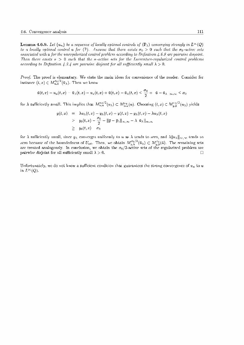
4.6. Convergence analysis 111
Lemma 4.6.9. Let f�ung be a sequence of locally optimal controls of (P�) converging strongly in L1(Q)to a locally optimal control �u for (P). Assume that there exists �0 > 0 such that the �0-active setsassociated with �u for the unregularized control problem according to De�nition 4.6.8 are pairwise disjoint.Then there exists � > 0 such that the �-active sets for the Lavrentiev-regularized control problemsaccording to De�nition 4.3.4 are pairwise disjoint for all su�ciently small � > 0.
Proof. The proof is elementary. We state the main ideas for convenience of the reader. Consider for
instance (t; x) 2M�0=2u;a (�u�). Then we know
�u(t; x)� ua(t; x) = �u�(t; x)� ua(t; x) + �u(t; x)� �u�(t; x) � �02+ k�u� �u�k1;1 � �0
for � su�ciently small. This implies that M�0=2u;a (�u�) �M�0
u;a(�u). Choosing (t; x) 2M�0=2y;b (�u�) yields
�y(t; x) = ��u�(t; x) + �y�(t; x) + �y(t; x)� �y�(t; x)� ��u�(t; x)
� yb(t; x)� �02� k�y � �y�k1;1 � �k�u�k1;1
� yb(t; x)� �0
for � su�ciently small, since �y� converges uniformly to �u as � tends to zero, and �k�u�k1;1 tends to
zero because of the boundedness of Uad. Then, we obtain M�0=2y;b (�u�) � M�0
y;b(�u). The remaining setsare treated analogously. In conclusion, we obtain the �0=2-active sets of the regularized problem arepairwise disjoint for all su�ciently small � > 0.
Unfortunately, we do not know a su�cient condition that guarantees the strong convergence of �un to �uin L1(Q).

5. A parabolic control problem with control
constraints
5.1. Introduction
In the previous chapter we have demonstrated that parabolic state constrained optimal control problemscan be handled well by regularization. The next step towards a complete analysis would be the discussionof a priori error estimates for a �nite element discretization of such problems. In the overview inChapter 1 we have already pointed out that the theory of a priori error estimates for parabolic controlproblems is far from complete. For state-constrained problems, the theoretical di�culties becomeobvious when pointing out that the adjoint state admits only the low regularity �p 2 L� (I;W 1;s
0 ())for some �; s 2 [1; 2), cf. also the introductory remarks in [107]. Then, standard arguments relying oninterpolation error estimates are not applicable, which makes a discussion of error estimates for state-constrained parabolic problems in full generality di�cult. One recent contribution to the analysis oflinear-quadratic state-constrained problems with �nitely many time-dependent controls has been madein [40]. For this setting, it was possible to prove uniform error estimates for the discrete states undernatural regularity assumption. Error estimates for the optimal control problem were then proven witha technique that avoids the use of error estimates for the adjoint state, cf. also [74] for elliptic problems.
Eventually, a rate of order O( 4plnhj(h 1
2 + k14 ) in two space dimensions and O(h 1
4 + h�14 k
14 ), in three
space dimensions has been proven for the error in the L2(I;Rm)-norm, where h is the spatial and kis the temporal discretization parameter. Linear-quadratic problems with arbitrary control functionsbut state constraints that were imposed pointwise in time and averaged in space have been analyzedin [100]. In the analysis, error estimates for the state equation in the L1(I; L2()) were needed andproven under regularity assumptions that can be expected for the considered problem class. Eventually,error estimates for the control in the L2-norm of order Oj ln kj(k 1
2 + h) have been obtained.
To our knowledge, there are no further contributions to the �nite element error analysis for parabolicstate-constrained optimal control problems. It is, however, known from elliptic problems that errorestimates for certain Lavrentiev regularized problems, i.e. without additional control-constraints, canbe obtained by transformation into a purely control constrained problem, cf. [73]. Yet, in the parabolicsetting even the results for control-constrained nonconvex problems are not as complete as in the ellipticsetting, where error estimates for problems with semilinear state equations have already been derivedin [8]. We mention again the results by Malanowski, [92], and Meidner and Vexler [102] for linearquadratic problems and Chrysa�nos, [33], for plain convergence results for problems with semilinearstate equation, and refer back to the Introduction in Chapter 1 for an overview. The main goal of thischapter therefore is to provide a priori error estimates for the �nite element discretization of a nonconvexcontrol-constrained optimal control problem. As in the elliptic setting from [73], we will motivate howcertain regularized state-constrained problems �t into this problem class as well. For that purpose, wewill brie y discuss Lavrentiev regularization for purely state-constrained problems. The correspondingresults are adapted to the nonconvex problems from the results for linear-quadratic setting that havebeen published by Tr�oltzsch and the author in [116].
113
114 5. A parabolic control problem with control constraints
The control-constrained problem is discretized by a discontinuous Galerkin scheme in time and a usualH1-conforming �nite element method in space. In [102] Meidner and Vexler analyzed the linear-quadratic counterpart of our model problem and proved error estimates that clearly separate the spatialand temporal discretization error for di�erent types of control discretization. We demonstrate how theseresults extend to the nonlinear setting, where we have to deal with three challenges: �rst we have totake into account corresponding local solutions. We have already seen in the last two chapters howthese can be handled. Moreover, a number of results on elliptic problems show how nonlinearities canbe treated, cf. also the overview in Chapters 1 and 3, so that a combination of these arguments withthe results from [102] seems promising. However, in the context of our model problem this involves asecond challenge, since the quadratic growth condition derived from SSC dictates the spaces in which�nite element error estimates have to be found. Third, we have to ensure that semidiscrete and dis-crete solutions to the nonlinear state equation (and adjoint equation and linearized equations) remainbounded in the L1(Q)-norm independent of the discretization parameters.
Let us mention again that the results on error estimates to be provided here have already been publishedin [118] by Vexler and the author for a model problem with slightly di�erent objective function. There,error estimates for cellwise constant control discretization have been discussed in detail and results forother types of discretization have been stated in a shorter form. In this thesis, we will discuss in detailthe error for controls that are discretized piecewise constant in time and bilinear in space. This, andalso the change in the objective function, are motivated by our interest in regularized state-constrainedproblems.
We point out that the notation in the papers [101, 102] and [118] di�er essentially from the notationused in this thesis. In particular, in the three mentioned papers the control was denoted by q, the stateby u, and the adjoint state by z, in contrast to our notation where u is the control, y is the state, andp is the adjoint state. Both notations are well-established, but this fact has to be kept in mind whenfollowing up on any given references.
5.2. Motivation by regularization
Before we turn to the analysis of error estimates for nonconvex control-constrained optimal control prob-lems, let us demonstrate how certain state constrained problems �t into the context of this chapter. Wewill apply Lavrentiev regularization to a purely state-constrained problem, discuss convergence issues,and eventually transform the regularized problem into a control-constrained problem. The followingresults on regularization, especially the convergence result, have to the most part been discussed inmore detail for linear quadratic problems in [116] by Tr�oltzsch and the author.
5.2.1. A control problem with pure pointwise state constraints
Relying on the same basic assumptions as in Chapter 4, suppose that the following purely state-constrained problem were given:
Minimize J(y; u) :=1
2
TZ0
Z
((y � yd)2 + �u2) dxdt (5.2.1a)
5.2. Motivation by regularization 115
subject to the PDE constraint
@ty ��y + d(t; x; y) = u in Q;y(0; �) = y0 in ;
y = 0 on �:(5.2.1b)
as well as the pointwise state constraints
ya � y(t; x) � yb a.e. in Q: (5.2.1c)
Assumption 5.2.1. Here, in accordance with Assumption 4.2.1, let � 2 R be a positive, �xed pa-rameter, and for simplicity let the bounds ya; yb be real numbers with ya < 0 < yb, ya � y0(x) � yb.Moreover, let the desired state yd be a function from L1(Q).
The analysis of Problem (5.2.1) provides yet some more challenges than the problems considered inChapter 4. In contrast to elliptic problems with mixed pointwise control-state constraints and nocontrol bounds we will encounter some regularity issues that we will comment on. First of all, we noticethat due to the missing control bounds there is no a priori reason to consider the controls in L1(Q).Due to the quadratic Tikhonov term ZZ
Q
�u2 dxdt
in the objective function an obvious candidate for the control space is L2(Q). Note, however, that forfunctions in L2(Q) and spatial domains of dimension larger than one, we only have the existence result ofTheorem 2.5.5 under somewhat more severe restrictions on the nonlinearities, i.e. global boundednessand global Lipschitz continuity. Theorem 2.5.5 on page 25 provides solvability in useful spaces, butnot continuity of the state { unless n = 1 and Theorem 2.5.6 is applicable. Consequently, the stateconstraints (5.2.1c) can only be formulated in the sense of Lp(Q), and Slater-type arguments cannotbe applied to obtain Lagrange multipliers unless we have better regularity properties of the optimalcontrol. This cannot be shown a priori. In fact, from the objective function it can only be shown that aminimizing sequence of controls is bounded in L2(Q), and then the existence of optimal controls followsin L2(Q), only, given that the set of feasible controls in L2(Q) is not empty.
On the other hand, there exist many examples where the optimal control has higher regularity thanjust L2(Q) even without explicitely prescribed control bounds, or if present constraints simply do notbecome active. At least, numerous academic examples can easily be constructed. One such example isgiven in Section 5.9.5. If a control u 2 Lp(Q), p � 2 is - locally or globally - optimal with respect to allL2(Q) functions, it is a fortiori also optimal if the search space is restricted to
U := Lp(Q); p > n=2 + 1:
Similar as before we obtain well-de�nedness of a control-to-state operator
Gp : Lp(Q)!W(0; T ) \ C( �Q); Gp(u) = y; p > n=2 + 1;
by Theorem 2.5.5, as well as the reduced objective function
fp : Lp(Q)! R; fp(u) := J(Gp(u); u) =
1
2
ZZQ
((Gp(u)� yd)2 + �u2) dxdt:
Here, the index p simply indicates that the control space is given by Lp(Q). It is known, cf. [144], thatGp is of class C2, where the derivatives take the same form as in Proposition 4.2.3. We simply assumethat a solution to the optimal control problem of the desired regularity exists.
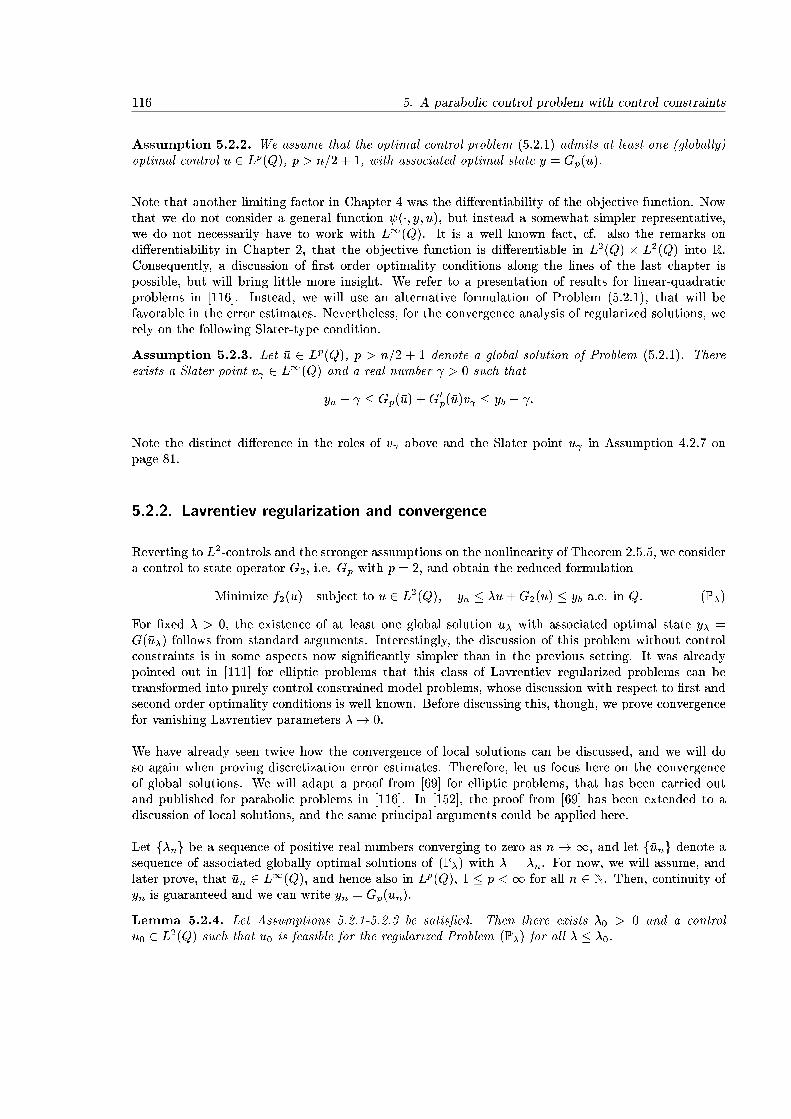
116 5. A parabolic control problem with control constraints
Assumption 5.2.2. We assume that the optimal control problem (5.2.1) admits at least one (globally)optimal control �u 2 Lp(Q), p > n=2 + 1, with associated optimal state �y = Gp(�u).
Note that another limiting factor in Chapter 4 was the di�erentiability of the objective function. Nowthat we do not consider a general function (�; y; u), but instead a somewhat simpler representative,we do not necessarily have to work with L1(Q). It is a well known fact, cf. also the remarks ondi�erentiability in Chapter 2, that the objective function is di�erentiable in L2(Q) � L2(Q) into R.Consequently, a discussion of �rst order optimality conditions along the lines of the last chapter ispossible, but will bring little more insight. We refer to a presentation of results for linear-quadraticproblems in [116]. Instead, we will use an alternative formulation of Problem (5.2.1), that will befavorable in the error estimates. Nevertheless, for the convergence analysis of regularized solutions, werely on the following Slater-type condition.
Assumption 5.2.3. Let �u 2 Lp(Q), p > n=2 + 1 denote a global solution of Problem (5.2.1). Thereexists a Slater point v 2 L1(Q) and a real number > 0 such that
ya + � Gp(�u) +G0p(�u)v � yb � :
Note the distinct di�erence in the roles of v above and the Slater point u in Assumption 4.2.7 onpage 81.
5.2.2. Lavrentiev regularization and convergence
Reverting to L2-controls and the stronger assumptions on the nonlinearity of Theorem 2.5.5, we considera control to state operator G2, i.e. Gp with p = 2, and obtain the reduced formulation
Minimize f2(u) subject to u 2 L2(Q); ya � �u+G2(u) � yb a.e. in Q: (P�)
For �xed � > 0, the existence of at least one global solution �u� with associated optimal state �y� =G(�u�) follows from standard arguments. Interestingly, the discussion of this problem without controlconstraints is in some aspects now signi�cantly simpler than in the previous setting. It was alreadypointed out in [111] for elliptic problems that this class of Lavrentiev regularized problems can betransformed into purely control constrained model problems, whose discussion with respect to �rst andsecond-order optimality conditions is well-known. Before discussing this, though, we prove convergencefor vanishing Lavrentiev parameters �! 0.
We have already seen twice how the convergence of local solutions can be discussed, and we will doso again when proving discretization error estimates. Therefore, let us focus here on the convergenceof global solutions. We will adapt a proof from [69] for elliptic problems, that has been carried outand published for parabolic problems in [116]. In [152], the proof from [69] has been extended to adiscussion of local solutions, and the same principal arguments could be applied here.
Let f�ng be a sequence of positive real numbers converging to zero as n ! 1, and let f�ung denote asequence of associated globally optimal solutions of (P�) with � = �n. For now, we will assume, andlater prove, that �un 2 L1(Q), and hence also in Lp(Q), 1 � p < 1 for all n 2 N. Then, continuity of�yn is guaranteed and we can write �yn = Gp(�un).
Lemma 5.2.4. Let Assumptions 5.2.1-5.2.3 be satis�ed. Then there exists �0 > 0 and a controlu0 2 L2(Q) such that u0 is feasible for the regularized Problem (P�) for all � � �0.
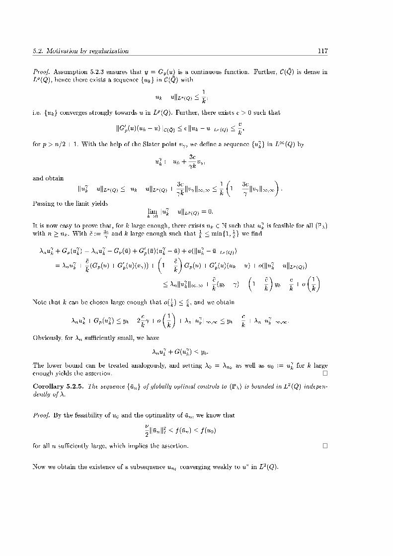
5.2. Motivation by regularization 117
Proof. Assumption 5.2.3 ensures that �y = Gp(�u) is a continuous function. Further, C( �Q) is dense inLp(Q), hence there exists a sequence fukg in C( �Q) with
kuk � �ukLp(Q) � 1
k;
i.e. fukg converges strongly towards �u in Lp(Q). Further, there exists c > 0 such that
kG0p(�u)(uk � �u)kC( �Q) � c kuk � �ukLp(Q) � c
k;
for p > n=2 + 1. With the help of the Slater point v , we de�ne a sequence fu kg in L1(Q) by
u k := uk +3c
kv ;
and obtain
ku k � �ukLp(Q) � kuk � �ukLp(Q) +3c
kkv k1;1 � 1
k
�1 +
3c
kv k1;1
�:
Passing to the limit yieldslimk!0
ku k � �ukLp(Q) = 0:
It is now easy to prove that, for k large enough, there exists nk 2 N such that u k is feasible for all (P�)with n � nk. With ~c := 3c
and k large enough such that 1k � minf1; 1~cg we �nd
�nu k +Gp(u
k) = �nu
k +Gp(�u) +G0p(�u)(u
k � �u) + o(ku k � �ukLp(Q))
= �nu k +
~c
k(Gp(�u) +G0p(�u)(v )) +
�1� ~c
k
�Gp(�u) +G0p(�u)(uk � �u) + o(ku k � �ukLp(Q))
� �nku kk1;1 +~c
k(yb � ) +
�1� ~c
k
�yb +
c
k+ o
�1
k
�Note that k can be chosen large enough that o( 1k ) � c
k , and we obtain
�nu k +Gp(u
k) � yb � 2
c
k + o
�1
k
�+ �nku kk1;1 � yb � c
k+ �nku kk1;1:
Obviously, for �n su�ciently small, we have
�nu k +G(u k) � yb:
The lower bound can be treated analogously, and setting �0 = �nk as well as u0 := u k for k largeenough yields the assertion.
Corollary 5.2.5. The sequence f�ung of globally optimal controls to (P�) is bounded in L2(Q) indepen-dently of �.
Proof. By the feasibility of u0 and the optimality of �un, we know that
�
2k�unk2I � f(�un) � f(u0)
for all n su�ciently large, which implies the assertion.
Now we obtain the existence of a subsequence �unk converging weakly to u� in L2(Q).

118 5. A parabolic control problem with control constraints
Lemma 5.2.6. Let f�unkg be the weakly converging subsequence of the sequence of globally optimalsolutions f�ung of (P�). The weak limit u
� 2 L2(Q) of f�unkg is feasible for Problem (5.2.1).
Proof. Since f�unkg is uniformly bounded in L2(Q) and f�ng tends to zero, we can assume w.l.o.g. thatk�n�unkk ! 0 and therefore �n�unk ! 0 pointwisely in Q, as n ! 1: Moreover, from the feasibility of�un for (P�), we obtain
ya � ��un +Gp(�un) � yb: (5.2.2)
From the compact embedding of W(0; T ) ,! L2(Q) we know that the optimal regularized states �yn :=Gp(�un) converge strongly towards y� := Gp(u
�) in L2(Q). Then, taking the limit in (5.2.2) yields theassertion, making use of the fact that [ya; yb] � L2(Q) is closed.
Theorem 5.2.7. Under Assumption 5.2.1-5.2.3, the sequence f�unkg converges strongly in L2(Q) to-wards u�, and u� is a global solution of (5.2.1).
Proof. Since �unk is globally optimal for (P�), we have
f(�unk) � f(u k)
for k large enough. Here, u k denotes the auxiliary control constructed in Lemma 5.2.4. By the lowersemi-continuity of f and the weak convergence of �unk towards u� we obtain for each k
f(u�) � lim infn!1
f(�unk) � lim supn!1
f(�unk) � f(u k):
For k !1 we arrive at
f(u�) � limk!1
f(u k) = f(�u) � f(u�);
hence f(u�) = f(�u), which implies optimality of u� for (5.2.1). It remains to show that the convergenceis strong in L2(Q). From the above, we know that
limn!1
f(�unk) = f(u�); (5.2.3)
and from the compactness of the embedding W(0; T ) ,! L2(Q) we further deduce that
limn!1
k�ynk � ydk2I = ky� � ydk2I ; (5.2.4)
where �ynk and y� denote the states associated with �unk and u�, respectively. Conditions (5.2.3) and(5.2.4) imply that
limn!1
k�unkk2I = ku�k2I :That, together with the weak convergence, implies strong convergence.
5.2.3. Transformation into a control constrained problem
Following [111], we now demonstrate how Problem (P�) can be transformed into a control constrainedproblem. For a �xed � > 0, we introduce the new control
w := �u+ y
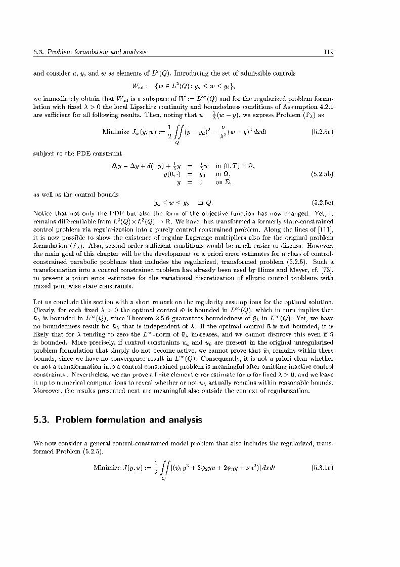
5.3. Problem formulation and analysis 119
and consider u, y, and w as elements of L2(Q). Introducing the set of admissible controls
Wad := fw 2 L2(Q) : ya � w � ybg;we immediately obtain that Wad is a subspace of W := L1(Q) and for the regularized problem formu-lation with �xed � > 0 the local Lipschitz continuity and boundedness conditions of Assumption 4.2.1are su�cient for all following results. Then, noting that u = 1
� (w � y), we express Problem (P�) as
Minimize Jw(y; w) :=1
2
ZZQ
(y � yd)2 +
�
�2(w � y)2 dxdt (5.2.5a)
subject to the PDE constraint
@ty ��y + d(�; y) + 1�y = 1
�w in (0; T )� ;y(0; �) = y0 in ;
y = 0 on �;(5.2.5b)
as well as the control boundsya � w � yb in Q: (5.2.5c)
Notice that not only the PDE but also the form of the objective function has now changed. Yet, itremains di�erentiable from L2(Q)�L2(Q)! R. We have thus transformed a formerly state-constrainedcontrol problem via regularization into a purely control constrained problem. Along the lines of [111],it is now possible to show the existence of regular Lagrange multipliers also for the original problemformulation (P�). Also, second order su�cient conditions would be much easier to discuss. However,the main goal of this chapter will be the development of a priori error estimates for a class of control-constrained parabolic problems that includes the regularized, transformed problem (5.2.5). Such atransformation into a control constrained problem has already been used by Hinze and Meyer, cf. [73],to present a priori error estimates for the variational discretization of elliptic control problems withmixed pointwise state constraints.
Let us conclude this section with a short remark on the regularity assumptions for the optimal solution.Clearly, for each �xed � > 0 the optimal control �w is bounded in L1(Q), which in turn implies that�u� is bounded in L1(Q), since Theorem 2.5.6 guarantees boundedness of �y� in L1(Q). Yet, we haveno boundedness result for �u� that is independent of �. If the optimal control �u is not bounded, it islikely that for � tending to zero the L1-norm of �u� increases, and we cannot disprove this even if �uis bounded. More precisely, if control constraints ua and ub are present in the original unregularizedproblem formulation that simply do not become active, we cannot prove that �u� remains within thesebounds, since we have no convergence result in L1(Q). Consequently, it is not a priori clear whetheror not a transformation into a control constrained problem is meaningful after omitting inactive controlconstraints . Nevertheless, we can prove a �nite element error estimate for �w for �xed � > 0, and we leaveit up to numerical computations to reveal whether or not �u� actually remains within reasonable bounds.Moreover, the results presented next are meaningful also outside the context of regularization.
5.3. Problem formulation and analysis
We now consider a general control-constrained model problem that also includes the regularized, trans-formed Problem (5.2.5).
Minimize J(y; u) :=1
2
ZZQ
[( 1y2 + 2 2yu+ 2 3y + �u2)] dxdt (5.3.1a)
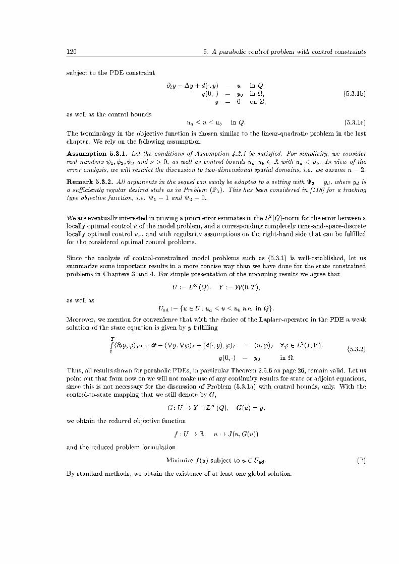
120 5. A parabolic control problem with control constraints
subject to the PDE constraint
@ty ��y + d(�; y) = u in Qy(0; �) = y0 in ;
y = 0 on �;(5.3.1b)
as well as the control boundsua � u � ub in Q: (5.3.1c)
The terminology in the objective function is chosen similar to the linear-quadratic problem in the lastchapter. We rely on the following assumption:
Assumption 5.3.1. Let the conditions of Assumption 4.2.1 be satis�ed. For simplicity, we considerreal numbers 1; 2; 3 and � > 0, as well as control bounds ua; ub 2 R with ua < ub. In view of theerror analysis, we will restrict the discussion to two-dimensional spatial domains, i.e. we assume n = 2.
Remark 5.3.2. All arguments in the sequel can easily be adapted to a setting with 3 = yd, where yd isa su�ciently regular desired state as in Problem (P�). This has been considered in [118] for a trackingtype objective function, i.e. 1 = 1 and 2 = 0.
We are eventually interested in proving a priori error estimates in the L2(Q)-norm for the error between alocally optimal control �u of the model problem, and a corresponding completely time-and-space-discretelocally optimal control �u�, and with regularity assumptions on the right-hand side that can be ful�lledfor the considered optimal control problems.
Since the analysis of control-constrained model problems such as (5.3.1) is well-established, let ussummarize some important results in a more concise way than we have done for the state constrainedproblems in Chapters 3 and 4. For simple presentation of the upcoming results we agree that
U := L1(Q); Y :=W(0; T );
as well asUad := fu 2 U : ua � u � ub a.e. in Qg:
Moreover, we mention for convenience that with the choice of the Laplace-operator in the PDE a weaksolution of the state equation is given by y ful�lling
TR0
h@ty; 'iV �;V dt+ (ry;r')I + (d(�; y); ')I = (u; ')I 8' 2 L2(I; V );
y(0; �) = y0 in :
(5.3.2)
Thus, all results shown for parabolic PDEs, in particular Theorem 2.5.6 on page 26, remain valid. Let uspoint out that from now on we will not make use of any continuity results for state or adjoint equations,since this is not necessary for the discussion of Problem (5.3.1a) with control bounds, only. With thecontrol-to-state mapping that we still denote by G,
G : U ! Y \ L1(Q); G(u) = y;
we obtain the reduced objective function
f : U ! R; u 7! J(u;G(u))
and the reduced problem formulation
Minimize f(u) subject to u 2 Uad: (P)
By standard methods, we obtain the existence of at least one global solution.

5.3. Problem formulation and analysis 121
Theorem 5.3.3. Let Assumption 5.3.1 be satis�ed. Then Problem (P) admits at least one optimalcontrol �u with associated state �y = G(�u).
Proof. This follows from [144, Theorem 5.7]. In particular, we point out that Uad is nonempty byassumption, and f is convex with respect to u since u only appears linearly in the term 2yu, andquadratically in �u2with positive parameter �.
We are now mainly interested in local solutions in the sense of L2(Q).
De�nition 5.3.4. A control �u 2 Uad is called a local solution of (P) in the sense of L2(Q) if thereexists a constant " > 0, such that the inequality
f(u) � f(�u)
is satis�ed for all u 2 Uad with k�u� ukI � ". We will refer to the associated optimal state as �y.
The treatment of �rst- and second-order optimality conditions is now very much simpli�ed by the factthat no pointwise state constraints are given. The analysis is standard procedure and can be foundin the monograph [144]. We will only collect what we need for our future analysis. In particular, wewill prove a more general second order su�cient condition not restricted to L1-neighborhoods. Wehave already argued that the objective function J is Fr�echet di�erentiable in L2(Q) � L2(Q), and weknow that the control-to-state operator G is twice di�erentiable with respect to the Lp(Q)-norm, withp > n=2 + 1. In our two-dimensional setting this implies p > 2. By the chain rule, we obtain thefollowing di�erentiability result for the reduced objective function f :
Lemma 5.3.5. The reduced objective function f is also of class C2. For arbitrary u; v; v1; v2 2 L1(Q)with associated y = G(u), ~y = G0(u)v, ~yi = G0(u)vi, i = 1; 2, as well as z := G00(u)[v1; v2], its �rst andsecond order derivative are given by
f 0(u)v =
ZZQ
( 1~yy + 2~yu+ 2yv + 3~y + �uv) dxdt
f 00(u)[v1; v2] =
ZZQ
( 1~y1~y2 + 1zy + 2~y2v2 + 2zu+ 2~y2v1 + 3z + �v1v2) dx dt:
Proof. The C2 regularity follows from known results for Nemytskii operators, cf. Chapter 2 and thechain rule. The form of the derivatives follow by straight-forward calculations, we refer also to, e. g.,[144] for details.
Now, we can formulate standard �rst order necessary optimality conditions with the help of a variationalinequality.
Lemma 5.3.6. Let �u 2 Uad be a local solution of (P) in the sense of De�nition 5.3.4. Then thefollowing variational inequality holds:
f 0(�u)(u� �u) � 0 8u 2 Uad: (5.3.3)
Proof. This is a standard result in optimal control for convex admissible sets. For a proof, we referagain to [144].
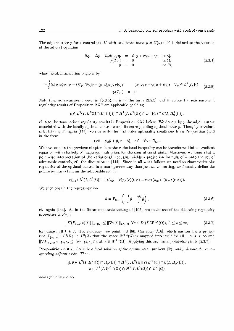
122 5. A parabolic control problem with control constraints
The adjoint state p for a control u 2 U with associated state y = G(u) 2 Y is de�ned as the solutionof the adjoint equation
�@tp��p+ @yd(�; y)p = 1y + 2u+ 3 in Q;p(T; �) = 0 in ;
p = 0 on �;(5.3.4)
whose weak formulation is given by
�TR0
h@tp; 'iV �;V + (r';rp)I + ('; @yd(�; y)p)I = ('; 1y + 2u+ 3)I 8' 2 L2(I; V )
p(T; �) = 0:
(5.3.5)
Note that no measures appear in (5.3.5); it is of the form (2.5.5) and therefore the existence andregularity results of Proposition 2.5.7 are applicable, yielding
p 2 L2(I;H2( \H10 ())) \H1(I; L2()) \ L1(Q) \ C(�I;H1
0 ());
cf. also the summarized regularity results in Proposition 5.3.7 below. We denote by �p the adjoint stateassociated with the locally optimal control �u and its corresponding optimal state �y. Then, by standardcalculations, cf. again [144], we can write the �rst order optimality conditions from Proposition 5.3.6in the form
(��u+ 2�y + �p; u� �u)I � 0 8u 2 Uad:
We have seen in the previous chapters how the variational inequality can be transformed into a gradientequation with the help of Lagrange multipliers for the control constraints. Moreover, we know that apointwise interpretation of the variational inequality yields a projection formula of �u onto the set ofadmissible controls, cf. the discussion in [144]. Since in all what follows we need to characterize theregularity of the optimal control in a more precise way than just an Lp-setting, we formally de�ne thepointwise projection on the admissible set by
PUad : L2(I; L2())! Uad; PUad(r)(t; x) = max(ua;2 (ub; r(t; x))):
We then obtain the representation
�u = PUad
��1
��p� 2
��y
�; (5.3.6)
cf. again [144]. As in the linear quadratic setting of [102], we make use of the following regularityproperties of PUad :
kr(PUad(v)(t))kLs() � krv(t)kLs() 8v 2 L2(I;W 1;s()); 1 � s � 1; (5.3.7)
for almost all t 2 I. For reference, we point out [80, Corollary A.6], which ensures for a projec-tion ~P[ua;ub] : L
2() ! L2() that the space W 1;s() is mapped into itself for all 1 � s � 1 and
kr ~P[ua;ub]vkLs() � krvkL2() for all v 2W 1;s(). Applying this argument pointwise yields (5.3.7).
Proposition 5.3.7. Let �u be a local solution of the optimization problem (P), and �p denote the corre-sponding adjoint state. Then
�y; �p 2 L2(I;H2() \H10 ()) \H1(I; L2()) \ L1(Q) \ C(�I;H1
0 ());
�u 2 L2(I;W 1;s()) \H1(I; L2()) \ L1(Q)
holds for any s <1.
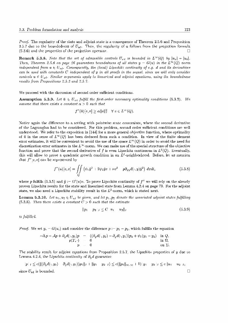
5.3. Problem formulation and analysis 123
Proof. The regularity of the state and adjoint state is a consequence of Theorem 2.5.6 and Proposition2.5.7 due to the boundedness of Uad. Then, the regularity of �u follows from the projection formula(5.3.6) and the properties of the projection operator.
Remark 5.3.8. Note that the set of admissible controls Uad is bounded in L1(Q) by juaj + jubj.Then, Theorem 2.5.6 on page 26 guarantees boundedness of all states y = G(u) in the L1(Q) normindependent from u 2 Uad. Consequently, the (local) Lipschitz continuity of e.g. d and its derivativescan be used with constants C independent of y in all proofs in the sequel, since we will only considercontrols u 2 Uad. Similar arguments apply to linearized and adjoint equations, using the boundednessresults from Propositions 2.5.2 and 2.5.7.
We proceed with the discussion of second order su�cient conditions.
Assumption 5.3.9. Let �u 2 Uad ful�ll the �rst-order necessary optimality conditions (5.3.3). Weassume that there exists a constant � > 0 such that
f 00(�u)[v; v] � �kvk2I 8 v 2 L1(Q):
Notice again the di�erence to a setting with pointwise state constraints, where the second derivativeof the Lagrangian had to be considered. For this problem, second order su�cient conditions are wellunderstood. We refer to the exposition in [144] for a more general objective function, where optimalityof �u in the sense of L1(Q) has been deduced from such a condition. In view of the �nite elementerror estimates, it will be convenient to avoid the use of the space L1(Q) in order to avoid the need fordiscretization error estimates in the L1-norm. We can make use of the special structure of the objectivefunction and prove that the second derivative of f is even Lipschitz continuous in L2(Q). Eventually,this will allow to prove a quadratic growth condition in an L2-neighborhood. Before, let us mentionthat f 00[v; v] can be represented by
f 00(u)[v; v] =
ZZQ
� 1~y
2 + 2 2~yv + �v2 � p@yyd(�; y)~y2�dxdt; (5.3.8)
where p ful�lls (5.3.5) and ~y := G0(u)v. To prove Lipschitz continuity of f 00 we will rely on the alreadyproven Lipschitz results for the state and linearized state from Lemma 4.2.4 on page 79. For the adjointstate, we also need a Lipschitz stability result in the L2-norm, which is stated next.
Lemma 5.3.10. Let u1; u2 2 Uad be given, and let p1; p2 denote the associated adjoint states ful�lling(5.3.5). Then there exists a constant C > 0 such that the estimate
kp1 � p2kI � C ku1 � u2kI (5.3.9)
is ful�lled.
Proof. We set yi = G(ui) and consider the di�erence p := p1 � p2, which ful�lls the equation
�@tp+Ap+ @yd(�; y1)p = ((@yd(�; y2)� @yd(�; y1))p2 + 1(y1 � y2) in Q;p(T; �) = 0 in ;
p = 0 on �:
The stability result for adjoint equations from Proposition 2.5.7, the Lipschitz properties of y due toLemma 4.2.4, the Lipschitz continuity of @yd guarantee
kpkI � c(k(@yd(�; y2)� @yd(�; y1))p2kI + ky1 � y2kI) � c(kp2k1;1 + 1)ky1 � y2kI � c ku1 � u2kI ;since Uad is bounded.
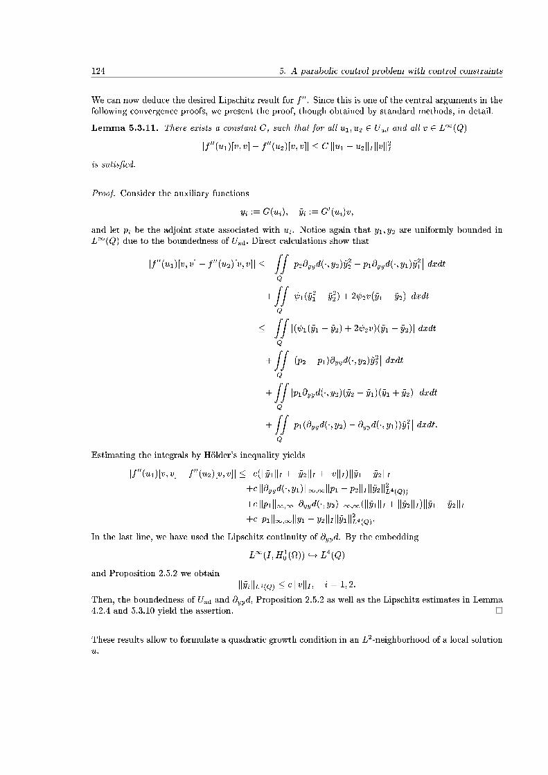
124 5. A parabolic control problem with control constraints
We can now deduce the desired Lipschitz result for f 00. Since this is one of the central arguments in thefollowing convergence proofs, we present the proof, though obtained by standard methods, in detail.
Lemma 5.3.11. There exists a constant C, such that for all u1; u2 2 Uad and all v 2 L1(Q)
jf 00(u1)[v; v]� f 00(u2)[v; v]j � C ku1 � u2kIkvk2Iis satis�ed.
Proof. Consider the auxiliary functions
yi := G(ui); ~yi := G0(ui)v;
and let pi be the adjoint state associated with ui. Notice again that y1; y2 are uniformly bounded inL1(Q) due to the boundedness of Uad: Direct calculations show that
jf 00(u1)[v; v]� f 00(u2)[v; v]j �ZZQ
��p2@yyd(�; y2)~y22 � p1@yyd(�; y1)~y21�� dxdt
+
ZZQ
�� 1(~y21 � ~y22) + 2 2v(~y1 � ~y2)�� dxdt
�ZZQ
j( 1(~y1 + ~y2) + 2 2v)(~y1 � ~y2)j dxdt
+
ZZQ
��(p2 � p1)@yyd(�; y2)~y22�� dxdt
+
ZZQ
jp1@yyd(�; y2)(~y2 � ~y1)(~y1 + ~y2)j dxdt
+
ZZQ
��p1(@yyd(�; y2)� @yyd(�; y1))~y21�� dxdt:
Estimating the integrals by H�older's inequality yields
jf 00(u1)[v; v]� f 00(u2)[v; v]j � c(k~y1kI + k~y2kI + kvkI)k~y1 � ~y2kI+c k@yyd(�; y1)k1;1kp1 � p2kIk~y2k2L4(Q))
+c kp1k1;1k@yyd(�; y2)k1;1(k~y1kI + k~y2kI)k~y1 � ~y2kI+ckp1k1;1ky1 � y2kIk~y1k2L4(Q):
In the last line, we have used the Lipschitz continuity of @yyd. By the embedding
L1(I;H10 ()) ,! L4(Q)
and Proposition 2.5.2 we obtaink~yikL4(Q) � c kvkI ; i = 1; 2:
Then, the boundedness of Uad and @yyd, Proposition 2.5.2 as well as the Lipschitz estimates in Lemma4.2.4 and 5.3.10 yield the assertion.
These results allow to formulate a quadratic growth condition in an L2-neighborhood of a local solution�u.
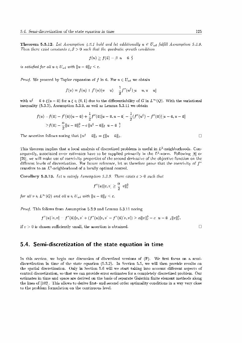
5.4. Semi-discretization of the state equation in time 125
Theorem 5.3.12. Let Assumption 4.2.1 hold and let additionally �u 2 Uad ful�ll Assumption 5.3.9.Then there exist constants "; � > 0 such that the quadratic growth condition
f(u) � f(�u) + �ku� �uk2Iis satis�ed for all u 2 Uad with ku� �ukI � ".
Proof. We proceed by Taylor expansion of f in �u. For u 2 Uad we obtain
f(u) = f(�u) + f 0(�u)(u� �u) +1
2f 00(u�)[u� �u; u� �u]
with u� = �u+ �(u� �u) for a � 2 (0; 1) due to the di�erentiability of G in L1(Q). With the variationalinequality (5.3.3), Assumption 5.3.9, as well as Lemma 5.3.11 we obtain
f(u) =f(�u) + f 0(�u)(u� �u) +1
2f 00(�u)[u� �u; u� �u] +
1
2(f 00(u�)� f 00(�u))[u� �u; u� �u]
�f(�u) + �
2ku� �uk2I � c ku� � �ukIku� �uk2I
The assertion follows noting that ku� � �ukI = �ku� �ukI .
This theorem implies that a local analysis of discretized problems is useful in L2-neighborhoods. Con-sequently, associated error estimates have to be supplied primarily in the L2-norm. Following [8] or[26], we will make use of coercivity properties of the second derivative of the objective function on thedi�erent levels of discretization. For future reference, let us therefore prove that the coercivity of f 00
transfers to an L2-neighborhood of a locally optimal control.
Corollary 5.3.13. Let �u satisfy Assumption 5.3.9. There exists " > 0 such that
f 00(u)[v; v] � �
2kvk2I
for all v 2 L1(Q) and all u 2 Uad with ku� �ukI � ":
Proof. This follows from Assumption 5.3.9 and Lemma 5.3.11 noting
f 00(u)[v; v] = f 00(�u)[v; v] + (f 00(u)[v; v]� f 00(�u)[v; v]) � �kvk2I � c ku� �ukIkvk2I :If " > 0 is chosen su�ciently small, the assertion is obtained.
5.4. Semi-discretization of the state equation in time
In this section, we begin our discussion of discretized versions of (P). We �rst focus on a semi-discretization in time of the state equation (5.3.2). In Section 5.5, we will then provide results onthe spatial discretization. Only in Section 5.6 will we start taking into account di�erent aspects ofcontrol discretization, so that we can provide error estimates for a completely discretized problem. Ourestimates in time and space are derived on the basis of separate Galerkin �nite element methods alongthe lines of [102]. This allows to derive �rst- and second order optimality conditions in a way very closeto the problem formulation on the continuous level.
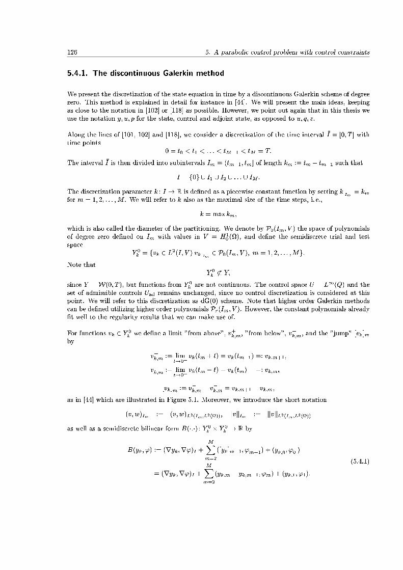
126 5. A parabolic control problem with control constraints
5.4.1. The discontinuous Galerkin method
We present the discretization of the state equation in time by a discontinuous Galerkin scheme of degreezero. This method is explained in detail for instance in [44]. We will present the main ideas, keepingas close to the notation in [102] or [118] as possible. However, we point out again that in this thesis weuse the notation y; u; p for the state, control and adjoint state, as opposed to u; q; z.
Along the lines of [101, 102] and [118], we consider a discretization of the time interval �I = [0; T ] withtime points
0 = t0 < t1 < : : : < tM�1 < tM = T:
The interval �I is then divided into subintervals Im = (tm�1; tm] of length km := tm � tm�1 such that
�I = f0g [ I1 [ I2 [ : : : [ IM :The discretization parameter k : I ! R is de�ned as a piecewise constant function by setting kjIm = kmfor m = 1; 2; : : : ;M . We will refer to k also as the maximal size of the time steps, i. e.,
k = max km;
which is also called the diameter of the partitioning. We denote by P0(Im; V ) the space of polynomialsof degree zero de�ned on Im with values in V = H1
0 (), and de�ne the semidiscrete trial and testspace
Y 0k = fvk 2 L2(I; V )jvkjIm 2 P0(Im; V ); m = 1; 2; : : : ;Mg:
Note thatY 0k 6� Y;
since Y =W(0; T ), but functions from Y 0k are not continuous. The control space U = L1(Q) and the
set of admissible controls Uad remains unchanged, since no control discretization is considered at thispoint. We will refer to this discretization as dG(0) scheme. Note that higher order Galerkin methodscan be de�ned utilizing higher order polynomials Pr(Im; V ). However, the constant polynomials already�t well to the regularity results that we can make use of.
For functions vk 2 Y 0k we de�ne a limit "from above", v+k;m, "from below", v�k;m, and the "jump" [vk]m
by
v+k;m := limt!0+
vk(tm + t) = vk(tm+1) =: vk;m+1;
v�k;m := limt!0+
vk(tm � t) = vk(tm) =: vk;m;
[vk]m := v+k;m � v�k;m = vk;m+1 � vk;m;
as in [44] which are illustrated in Figure 5.1. Moreover, we introduce the short notation
(v; w)Im := (v; w)L2(Im;L2()); kvkIm := kvkL2(Im;L2())as well as a semidiscrete bilinear form B(�:�) : Y 0
k � Y 0k ! R by
B(yk; ') := (ryk;r')I +MXm=2
([yk]m�1; '+m�1) + (y+k;0; '
+0 )
= (ryk;r')I +MXm=2
(yk;m � yk;m�1; 'm) + (yk;1; '1):
(5.4.1)

5.4. Semi-discretization of the state equation in time 127
Im
tm�1 tm tm+1
v�
k;m
[vk]m
v+
k;m
vk
Figure 5.1.: Notation for the dG(0) method
This can also be expressed as
B(yk; ') = (ryk;r')I +M�1Xm=1
([yk]m; '+m) + (yk;1; '1):
No value of ' is required at t = 0. We refer to [47] for further details as well as an equivalent formulationof the dG(0) scheme. The dG(0) semidiscretization of the state equation (5.3.2) for �xed control u 2 Unow reads as follows:
Find a state yk = yk(u) 2 Y 0k such that
B(yk; ') + (d(�; yk); ')I = (u; ')I + (y0; '1) 8' 2 Y 0k : (5.4.2)
Note that we do not require yk to ful�ll the initial condition exactly. To explain this, consider the caseM = 1, i.e. a setting with only one time interval (t0; t1] = (0; T ]. Then, we obtain the semidiscretestate equation
(ryk;r')I + (yk; ') + (d(�; yk); ')I = (u; ')I + (y0; ') 8' 2 P0(I; V ); (5.4.3)
which is equivalent to
(ryk;r')I + (yk � y0; ') + (d(�; yk); ')I = (u; ')I 8' 2 P0(I; V ): (5.4.4)
Since both the state space and the test space are the same, i.e. constant polynomials in time withvalues in V = H1
0 (), yk cannot be expected to ful�ll the initial condition
yk(0; x) = y0(x);
exactly, as this would lead to an overdetermined system. Instead, the term
(yk � y0; ')

128 5. A parabolic control problem with control constraints
in (5.4.4) imposes the initial condition in a variational sense. For M > 1, successive application of thismethod on the time intervals Im, m = 1; : : : ;M explains the jump terms in the de�nition of B. Werefer again to [44].
For later use of the bilinear form for the adjoint equation we point out that for '; vk 2 Y 0k , B ful�lls
B('; vk) = (r';rvk)I +M�1Xm=1
(['m]; v+k;m) + ('1; vk;1)
= (r';rvk)I +M�1Xm=1
('m+1 � 'm; vk;m+1) + ('1; vk;1)
= (r';rvk)I �M�1Xm=1
('m; vk;m+1 � vk;m) +
M�1Xm=1
('m+1; vk;m+1)
�M�1Xm=1
('m; vk;m) + ('1; vk;1)
= (r';rvk)I �M�1Xm=1
('�m; [vk]m) + ('�M ; v�k;M )
= (r';rvk)I �M�1Xm=1
('�m; [vk]m) + ('M ; vk;M );
(5.4.5)
cf. [101].
For all what follows, we point out again that the spatial dimension n = 2 is considered. The reason forthis lies in regularity results for the space-time-discretized state, but we will adapt all further discussionto this setting. In principal, we will proceed with the same or similar steps as for the continuousproblem. We will �rst discuss existence, regularity, and stability estimates for the semi-discrete stateequation, where we cannot easily make use of available results. Once these are available, optimalityconditions of the semi-discrete control problem can be discussed, along with a discussion of linearizedand adjoint equations. Then, a discretization error of uncontrolled equations is derived, that willeventually determine the temporal error in the optimal controls.
5.4.2. Existence results and stability estimates for the semi-discrete state
equation
The properties of the semi-discrete state equation essentially in uence the analysis of the semidiscreteoptimal control problem. We will therefore very carefully discuss the semi-discrete equations. Onceresults comparable to the continuous level are available we can proceed with the analysis of the semidis-crete optimal control problem. Most stability estimates needed can be obtained extending results forlinear equations from [101], cf. also [45, 46]. We begin with plain existence and uniqueness, as well asboundedness in L1(Q) independently of the discretization. In some sense, this is the central argumentin the following proofs.
Theorem 5.4.1. Let Assumption 5.3.1 be satis�ed. Then, for every �xed control u 2 U and initialstate y0 2 V \ L1(Q), the semidiscrete state equation (5.4.2) admits a unique semidiscrete solutionyk 2 Y 0
k \ L1(Q).

5.4. Semi-discretization of the state equation in time 129
Proof. The existence of a solution follows by applying standard arguments from elliptic theory to thesystem of semilinear elliptic PDEs for each time interval obtained after semidiscretization in time. It issu�cient to prove the assertion on the interval I1, cf. also [138]. We obtain the formulation
k1(ryk;1;r'1) + (yk;1; '1) + (d(t; x; yk;1); '1)I1 = (u; '1)I1 + (y0; '1) 8'1 2 V;where u and y0 are given. With the auxiliary functions
~d(x; yk;1) :=
ZI1
d(t; x; yk;1(x))dt;
~u(x) :=
ZI1
u(t; x)dt;
this yields
k1(ryk;1;r'1) + (yk;1; '1) + ( ~d(�; yk;1); '1) = (~u; '1) + (y0; '1) 8'1 2 V: (5.4.6)
Clearly, the monotonicity and Lipschitz properties of d remain valid for ~d, and ~u is a function fromL1(). We can apply Theorem 2.4.6 to this elliptic boundary value problem and for each y0; ~u 2 L2()we obtain a unique solution yk;1 2 H1
0 ()\L1(). This argumentation can successively be applied toall time intervals, and we obtain the existence of a semidiscrete solution yk 2 Y 0
k \L1(Q) to (5.4.2).
The existence of a unique solution yk 2 L1(Q) is the starting point for our analysis, but not su�cient forlater results. For the stability and error estimates to come, we will need to rely on boundedness estimatesthat do not depend on the discretization parameter k. Yet, applying elliptic stability arguments to(5.4.6) will lead to an estimate which is proportional to 1=k.
In elliptic problems, boundedness of the discrete states yh in L1() can be obtained with the helpof an inverse estimate between the norms on L1() and L2() for cellwise polynomials, once anerror estimate in the L2-norm depending on the spatial discretization parameter h is established understrong assumptions on the appearing nonlinearities. These strong assumptions can be weakened afterboundedness of the discrete states is obtained, cf. [23] for a detailed discussion. This procedure is noteasily transferable to parabolic problems, since an estimate in the L1(Q) norm on the whole space-time-domain is needed. In [46], error estimates in the L1(I �)-norm have been shown for linear problems,but the regularity assumptions are too strong for our optimal control problem. In order to obtain aplain boundedness result independent of k, we will continue di�erently and apply Stampacchia's methodto the semidiscrete state equation (5.4.2).
Theorem 5.4.2. Let the conditions from Theorem 5.4.1 hold and note in particular that the spatialdimension n = 2. Then, the solution yk satis�es the boundedness result
kykk1;1 � C (kukLp(Q) + kd(�; 0)kLp(Q) + ky0k1)
for every p > 2 and a constant C independent of the discretization parameter k.
Proof. We follow closely the proof of [144, Theorem 4.5] for elliptic equations. Let therefore b � ky0k1be a real number and choose a test-function vk 2 Y 0
k such that
vk;m =
8<:yk;m � b on +
k;m(b) := fx 2 : yk;m(x) > bgyk;m + b on �k;m(b) := fx 2 : yk;m(x) < �bg0 on n (+
k;m(b) [ �k;m(b)):
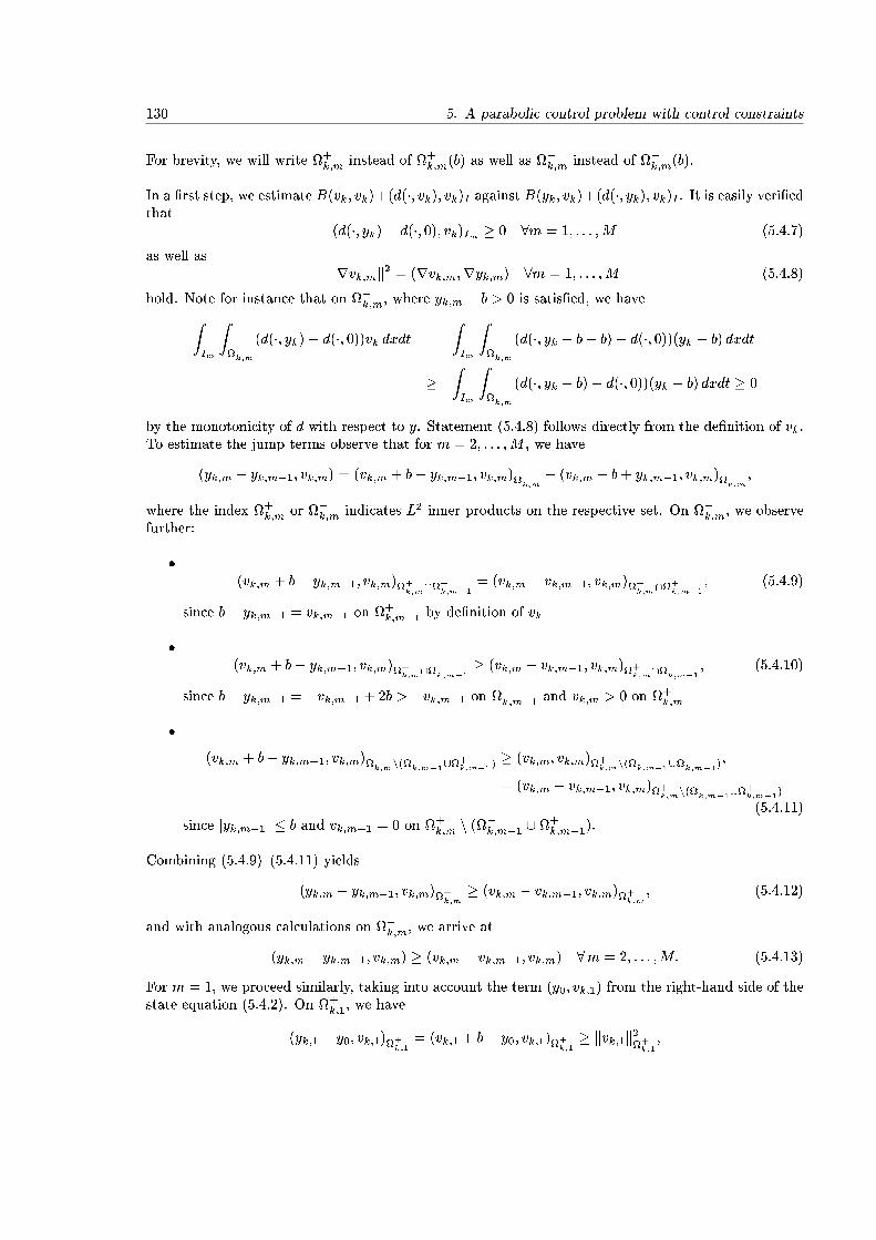
130 5. A parabolic control problem with control constraints
For brevity, we will write +k;m instead of +
k;m(b) as well as �k;m instead of �k;m(b).
In a �rst step, we estimate B(vk; vk)+(d(�; vk); vk)I against B(yk; vk)+(d(�; yk); vk)I . It is easily veri�edthat
(d(�; yk)� d(�; 0); vk)Im � 0 8m = 1; : : : ;M (5.4.7)
as well askrvk;mk2 = (rvk;m;ryk;m) 8m = 1; : : : ;M (5.4.8)
hold. Note for instance that on +k;m, where yk;m � b > 0 is satis�ed, we haveZ
Im
Z+k;m
(d(�; yk)� d(�; 0))vk dxdt =
ZIm
Z+k;m
(d(�; yk � b+ b)� d(�; 0))(yk � b) dxdt
�ZIm
Z+k;m
(d(�; yk � b)� d(�; 0))(yk � b) dxdt � 0
by the monotonicity of d with respect to y. Statement (5.4.8) follows directly from the de�nition of vk.To estimate the jump terms observe that for m = 2; : : : ;M , we have
(yk;m � yk;m�1; vk;m) = (vk;m + b� yk;m�1; vk;m)+k;m
+ (vk;m � b+ yk;m�1; vk;m)�k;m
;
where the index +k;m or �k;m indicates L2 inner products on the respective set. On +
k;m, we observefurther:
�(vk;m + b� yk;m�1; vk;m)+
k;m\+
k;m�1= (vk;m � vk;m�1; vk;m)+
k;m\+
k;m�1; (5.4.9)
since b� yk;m�1 = vk;m�1 on +k;m�1 by de�nition of vk
�(vk;m + b� yk;m�1; vk;m)+
k;m\�
k;m�1� (vk;m � vk;m�1; vk;m)+
k;m\�
k;m�1; (5.4.10)
since b� yk;m�1 = �vk;m�1 + 2b > �vk;m�1 on �k;m�1 and vk;m > 0 on +k;m
�(vk;m + b� yk;m�1; vk;m)+
k;mn(�
k;m�1[+k;m�1)
� (vk;m; vk;m)+k;m
n(�k;m�1[
+k;m�1)
;
= (vk;m � vk;m�1; vk;m)+k;m
n(�k;m�1[
+k;m�1)
(5.4.11)since jyk;m�1j � b and vk;m�1 = 0 on +
k;m n (�k;m�1 [ +k;m�1).
Combining (5.4.9){(5.4.11) yields
(yk;m � yk;m�1; vk;m)+k;m
� (vk;m � vk;m�1; vk;m)+k;m
; (5.4.12)
and with analogous calculations on �k;m, we arrive at
(yk;m � yk;m�1; vk;m) � (vk;m � vk;m�1; vk;m) 8m = 2; : : : ;M: (5.4.13)
For m = 1, we proceed similarly, taking into account the term (y0; vk;1) from the right-hand side of thestate equation (5.4.2). On +
k;1, we have
(yk;1 � y0; vk;1)+k;1
= (vk;1 + b� y0; vk;1)+k;1� kvk;1k2+
k;1
;

5.4. Semi-discretization of the state equation in time 131
where the last inequality follows from the fact that b � ky0k1 and vk;1 > 0 on +k;1. Together with
analogous calculations on �k;1, this yields
(yk;1 � y0; vk;1) � kvk;1k2: (5.4.14)
From (5.4.7),(5.4.8),(5.4.13), and (5.4.14) we obtain
B(vk; vk) � B(yk; vk)� (y0; vk;1) � (u� d(�; 0); vk)I ;which in particular implies
kvkk2L1(I;L2())\L2(I;H10 ())
� (u� d(�; 0); vk)I ; (5.4.15)
as we will discuss in more detail in the proof of Theorem 5.4.5 below.
In the second step of the proof, we estimate (5.4.15) further. Note that we have the embeddings
H10 () ,! L�(); 8 1 < � <1
as well asL1(I; L2()) ,! L�(I; L2()); 8 1 < � <1
since is two dimensional, cf. [1]. Then, known interpolation error estimates, cf. [139], yield
L2(I;H10 ()) \ L�(I; L2()) ,! Lrs(I; [H1
0 (); L2()]s) ,! Lrs(I; Lqs())
with1
rs=
1� s
2+s
�;
1
qs=
1� s
�+s
2; s 2 (0; 1):
Choosing s = 12 yields
rs = qs =4�
2 + �< 4;
which is monotonically increasing in �. Hence, we deduce that
L1(I; L2()) \ L2(I;H10 ()) ,! L� (Q) (5.4.16)
is satis�ed for any positive real number � < 4. To eventually be able to apply Stampacchia's Lemmawe point out that for all p > 2 there exist � > 1 and p0 > 0 such that 1
p +1p0 = 1 and p0 = �
2� is satis�ed.
With the embedding (5.4.16) as well as estimate (5.4.15) we obtain
kvkk2L� (Q) � ckvkk2L1(I;L2())\L2(I;H10 ())
� c ku� d(�; 0)kLp(Q)kvkkLp0 (Q) (5.4.17)
where we used H�older's inequality. De�ning I(b) � Q as
I(b) := f(t; x) 2 Q j jyk(t; x)j > bg;and denoting by �I(b) its characteristic function we obtain from (5.4.17)
kvkk2L� (Q) � c ku� d(�; 0)kLp(Q)kvkkLp0 (Q)
= c ku� d(�; 0)kLp(Q) ��ZZ
Q
�I(b) jvkjp0
dxdt
� 1p0
� c ku� d(�; 0)kLp(Q)kvkkL2p0 (Q)jI(b)j12p0 ;
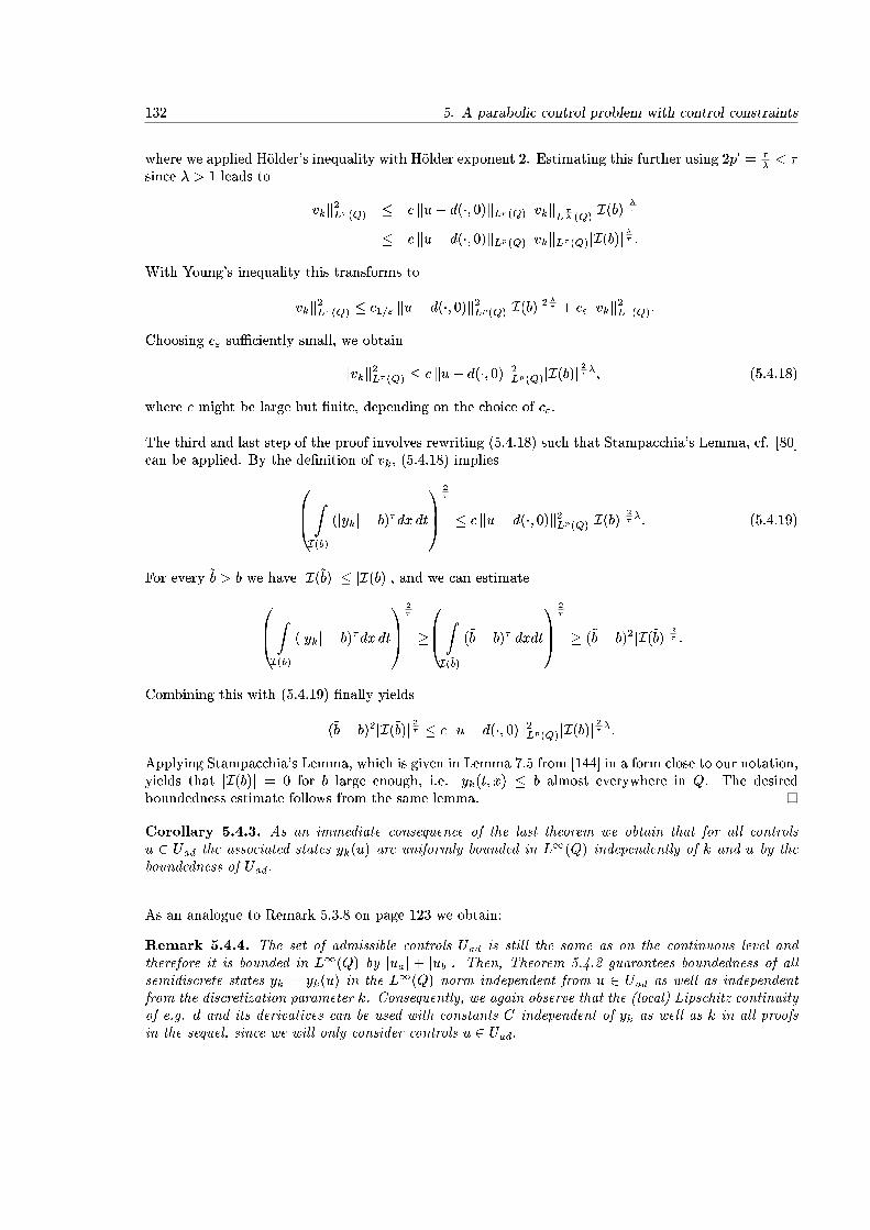
132 5. A parabolic control problem with control constraints
where we applied H�older's inequality with H�older exponent 2. Estimating this further using 2p0 = �� < �
since � > 1 leads to
kvkk2L� (Q) � c ku� d(�; 0)kLp(Q)kvkkL �� (Q)
jI(b)j��� c ku� d(�; 0)kLp(Q)kvkkL� (Q)jI(b)j�� :
With Young's inequality this transforms to
kvkk2L� (Q) � c1=" ku� d(�; 0)k2Lp(Q)jI(b)j2�� + c"kvkk2L� (Q):
Choosing c" su�ciently small, we obtain
kvkk2L� (Q) � c ku� d(�; 0)k2Lp(Q)jI(b)j2��; (5.4.18)
where c might be large but �nite, depending on the choice of c".
The third and last step of the proof involves rewriting (5.4.18) such that Stampacchia's Lemma, cf. [80]can be applied. By the de�nition of vk, (5.4.18) implies0B@ Z
I(b)
(jykj � b)�dx dt
1CA2�
� c ku� d(�; 0)k2Lp(Q)jI(b)j2��: (5.4.19)
For every ~b > b we have jI(~b)j � jI(b)j, and we can estimate0B@ ZI(b)
(jykj � b)�dx dt
1CA2�
�
0B@ ZI(~b)
(~b� b)� dxdt
1CA2�
� (~b� b)2jI(~b)j 2� :
Combining this with (5.4.19) �nally yields
(~b� b)2jI(~b)j 2� � c ku� d(�; 0)k2Lp(Q)jI(b)j2��:
Applying Stampacchia's Lemma, which is given in Lemma 7.5 from [144] in a form close to our notation,yields that jI(b)j = 0 for b large enough, i.e. yk(t; x) � b almost everywhere in Q. The desiredboundedness estimate follows from the same lemma.
Corollary 5.4.3. As an immediate consequence of the last theorem we obtain that for all controlsu 2 Uad the associated states yk(u) are uniformly bounded in L1(Q) independently of k and u by theboundedness of Uad.
As an analogue to Remark 5.3.8 on page 123 we obtain:
Remark 5.4.4. The set of admissible controls Uad is still the same as on the continuous level andtherefore it is bounded in L1(Q) by juaj + jubj. Then, Theorem 5.4.2 guarantees boundedness of allsemidiscrete states yk = yk(u) in the L1(Q) norm independent from u 2 Uad as well as independentfrom the discretization parameter k. Consequently, we again observe that the (local) Lipschitz continuityof e.g. d and its derivatives can be used with constants C independent of yk as well as k in all proofsin the sequel, since we will only consider controls u 2 Uad.
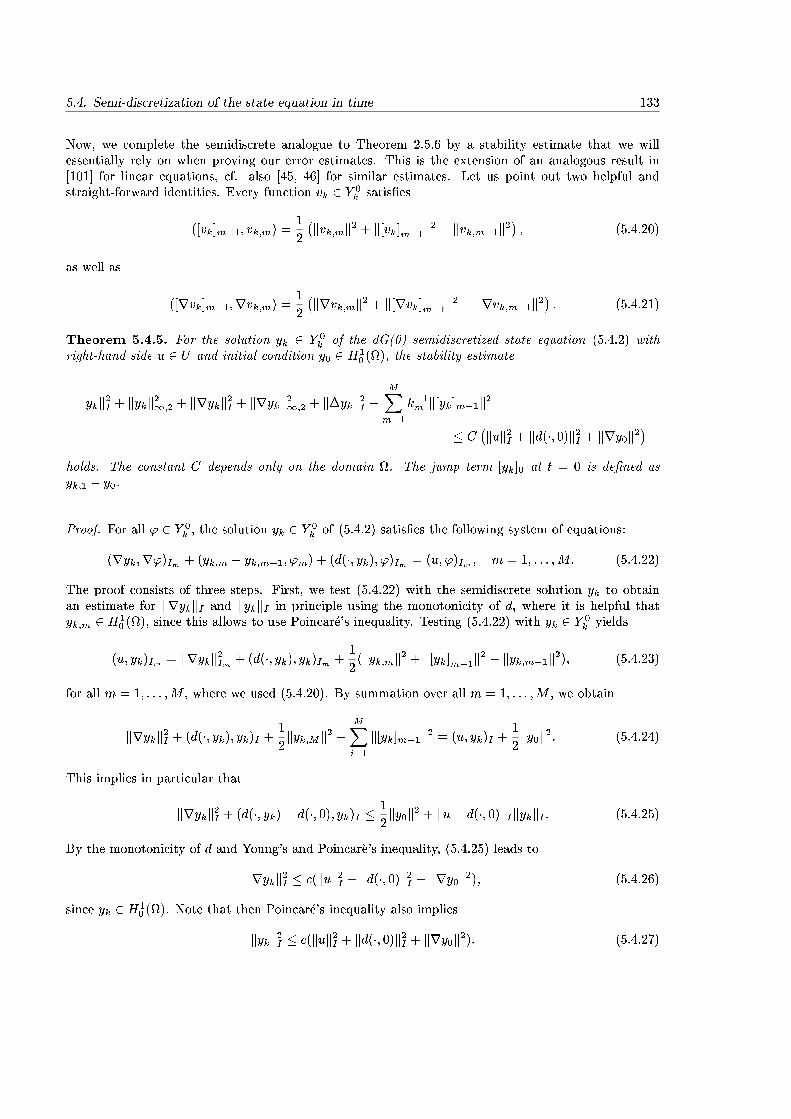
5.4. Semi-discretization of the state equation in time 133
Now, we complete the semidiscrete analogue to Theorem 2.5.6 by a stability estimate that we willessentially rely on when proving our error estimates. This is the extension of an analogous result in[101] for linear equations, cf. also [45, 46] for similar estimates. Let us point out two helpful andstraight-forward identities. Every function vk 2 Y 0
k satis�es
([vk]m�1; vk;m) =1
2
�kvk;mk2 + k[vk]m�1k2 � kvk;m�1k2�; (5.4.20)
as well as
([rvk]m�1;rvk;m) = 1
2
�krvk;mk2 + k[rvk]m�1k2 � krvk;m�1k2�: (5.4.21)
Theorem 5.4.5. For the solution yk 2 Y 0k of the dG(0) semidiscretized state equation (5.4.2) with
right-hand side u 2 U and initial condition y0 2 H10 (), the stability estimate
kykk2I + kykk21;2 + krykk2I + krykk21;2 + k�ykk2I +MXm=1
k�1m k[yk]m�1k2
� C�kuk2I + kd(�; 0)k2I + kry0k2
�holds. The constant C depends only on the domain . The jump term [yk]0 at t = 0 is de�ned asyk;1 � y0.
Proof. For all ' 2 Y 0k , the solution yk 2 Y 0
k of (5.4.2) satis�es the following system of equations:
(ryk;r')Im + (yk;m � yk;m�1; 'm) + (d(�; yk); ')Im = (u; ')Im ; m = 1; : : : ;M: (5.4.22)
The proof consists of three steps. First, we test (5.4.22) with the semidiscrete solution yk to obtainan estimate for krykkI and kykkI in principle using the monotonicity of d, where it is helpful thatyk;m 2 H1
0 (), since this allows to use Poincar�e's inequality. Testing (5.4.22) with yk 2 Y 0k yields
(u; yk)Im = krykk2Im + (d(�; yk); yk)Im +1
2(kyk;mk2 + k[yk]m�1k2 � kyk;m�1k2); (5.4.23)
for all m = 1; : : : ;M , where we used (5.4.20). By summation over all m = 1; : : : ;M , we obtain
krykk2I + (d(�; yk); yk)I + 1
2kyk;Mk2 +
MXi=1
k[yk]m�1k2 = (u; yk)I +1
2ky0k2: (5.4.24)
This implies in particular that
krykk2I + (d(�; yk)� d(�; 0); yk)I � 1
2ky0k2 + ku� d(�; 0)kIkykkI : (5.4.25)
By the monotonicity of d and Young's and Poincar�e's inequality, (5.4.25) leads to
krykk2I � c(kuk2I + kd(�; 0)k2I + kry0k2); (5.4.26)
since yk 2 H10 (). Note that then Poincar�e's inequality also implies
kykk2I � c(kuk2I + kd(�; 0)k2I + kry0k2): (5.4.27)

134 5. A parabolic control problem with control constraints
In the second step, we estimate the terms k�ykk2I andMPm=1
k�1m k[yk]m�1k2 by applying Theorem 4.1
from [101] to the linear equation
B(yk; ') = (u� d(�; yk); ')I + (y0; '1); 8' 2 Y 0k : (5.4.28)
Then, we know that
k�ykk2I +MXm=1
k�1m k[yk]m�1k2 � c�ku� d(�; yk)k2I + kry0k2
�; (5.4.29)
which follows in principle from testing (5.4.2) with ' = [yk]m�1 2 P0(I;H10 ()) as well as integrating
(5.4.2) by parts in space to be able to test with ' = ��yk 2 P0(I; L2()). For more details, we refer
to [101]. The right-hand side of (5.4.29) can be estimated by
ku� d(�; yk)k2I � c(kuk2I + kd(�; 0)k2I + kd(�; 0)� d(�; yk)k2I) � c�kuk2I + kd(�; 0)k2I + kykk2I
�(5.4.30)
by the local Lipschitz continuity of d and the fact that yk is uniformly bounded for all u 2 Uad due toTheorem 5.4.2. Inserting (5.4.27) yields the proposed estimate for k�ykkI and the jump terms.
In a third step, we need to estimate kykk1;2 and krykk1;2. In fact, the proof in [101, Theorem4.1] already provides this (for linear equations). Consider again the linear equation (5.4.28). Partialintegration in space and testing with ' = ��yk yields
k�ykk2Im + ([ryk]m�1;ryk;m) = (u� d(�; 0) + d(�; 0)� d(�; yk);��yk)Im (5.4.31)
for all m = 1; : : : ;M . We refer to [101] for further details. Using (5.4.21) and the Lipschitz property ofd and summation over all m yield
1
2kryk;Mk2 + 1
2
MXm=1
k[ryk]m�1k2 + k�ykk2I � ku� d(�; 0)kIk�ykkI + c kykkIk�ykkI + 1
2kry0k2I :
With Young's inequality and (5.4.27) this implies
kryk;Mk2 +MXm=1
k[ryk]m�1k2 � c�kuk2I + kry0k2 + 1
�:
Since now each of the jump terms and therefore also their maximum is bounded, this yields the desiredestimate for kykk1;2 and krykk1;2 after again applying Poincar�e's inequality.
Remark 5.4.6. Note that elliptic regularity and the fact that is convex and polygonal imply
kr2ykk2I � ck�ykk2I � C�kuk2I + kd(�; 0)k2I + kry0k2
�:
5.4.3. The optimal control problem with semidiscrete state equation
The existence and regularity results for the semidiscrete state equation allow to treat a time-discreteversion of the model problem by the same means as on the continuous level. We start with the de�nitionof a control-to-state operator and a reduced objective function.
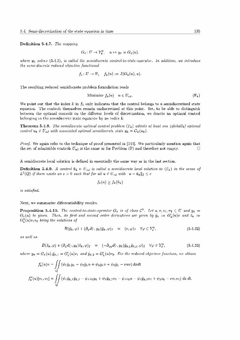
5.4. Semi-discretization of the state equation in time 135
De�nition 5.4.7. The mapping
Gk : U ! Y 0k ; u 7! yk = Gk(u);
where yk solves (5.4.2), is called the semidiscrete control-to-state-operator. In addition, we introducethe semi-discrete reduced objective functional
fk : U ! R; fk(u) := J(Gk(u); u):
The resulting reduced semidiscrete problem formulation reads
Minimize fk(u) u 2 Uad: (Pk)
We point out that the index k in fk only indicates that the control belongs to a semidiscretized stateequation. The controls themselves remain undiscretized at this point. Yet, to be able to distinguishbetween the optimal controls on the di�erent levels of discretization, we denote an optimal controlbelonging to the semidiscrete state equation by an index k.
Theorem 5.4.8. The semidiscrete optimal control problem (Pk) admits at least one (globally) optimalcontrol �uk 2 Uad with associated optimal semidiscrete state �yk = Gk(�uk).
Proof. We again refer to the technique of proof presented in [144]. We particularly mention again thatthe set of admissible controls Uad is the same as for Problem (P) and therefore not empty.
A semidiscrete local solution is de�ned in essentially the same way as in the last section.
De�nition 5.4.9. A control �uk 2 Uad is called a semidiscrete local solution to (Pk) in the sense ofL2(Q) if there exists an " > 0 such that for all u 2 Uad with ku� �ukkI � "
fk(u) � fk(�uk)
is satis�ed.
Next, we summarize di�erentiability results.
Proposition 5.4.10. The control-to-state-operator Gk is of class C2. Let u; v; v1; v2 2 U and yk =Gk(u) be given. Then, its �rst and second order derivatives are given by ~yk := G0k(u)v and ~zk :=G00k(u)v1v2 being the solutions of
B(~yk; ') + (@yd(�; yk)~yk; ')I = (v; ')I 8' 2 Y 0k ; (5.4.32)
as well as
B(~zk; ') + (@yd(�; yk)~zk; ')I = (�@yyd(�; yk)~yk;1~yk;2; ')I 8' 2 Y 0k ; (5.4.33)
where yk = Gk(u),~yk;1 = G0k(u)v1 and ~yk;2 = G0k(u)v2. For the reduced objective function, we obtain
f 0k(u)v =
ZZQ
( 1~ykyk + 2~yku+ 2ykv + 3~yk + �uv) dxdt
f 00k (u)[v1; v2] =
ZZQ
( 1~yk;1~yk;2 + 1zkyk + 2~yk;2v2 + 2zku+ 2~yk;2v1 + 3zk + �v1v2) dx dt:

136 5. A parabolic control problem with control constraints
Proof. The proof follows as in Theorems 5.9, 5.15, and 5.16 in [144] for the control-to-state operator.By the di�erentiability of J in L2(Q) � L2(Q) and the chain rule, we know that f is of class C2.Straight-forward calculations yield the precise formulation of the derivatives.
It is clear that the stability estimates of Theorems 5.4.2 and 5.4.5 are also valid for linearized semidiscretestate equations:
Lemma 5.4.11. Let u 2 Uad and v 2 U be given and denote by ~yk the semidiscrete linearized state~yk = G0k(u)v. Then there exists a constant c > 0 independent of k and u 2 Uad such that
k~ykkI �c kvkI (5.4.34)
k~ykk1;1 �c kvkLp(Q) (5.4.35)
k~ykk1;2 + kr~ykk1;2 �c kvkI (5.4.36)
holds for any p > 2.
Note in particular that the constant c are also independent of the term @yd(�; yk) appearing in thelinearized equations, since yk is uniformly bounded for all u 2 Uad, independent of k.
For u 2 U and yk := Gk(u) we de�ne the semidiscrete adjoint state pk = pk(u) 2 Y 0k as the solution of
the semidiscrete adjoint equation
B('; pk) + ('; @yd(�; yk)pk) = ('; 1yk + 2u+ 3)I 8' 2 Y 0k : (5.4.37)
We denote by �pk the adjoint state associated with the locally optimal control �uk and its correspondingoptimal state �yk. For a more general right-hand side g 2 L1(Q) and terminal condition pT 2 H1
0 ()we consider the semidiscretized dual equation
B('; pk) + ('; @yd(�; yk(u))pk)I = ('; g)I + ('M ; pT ) 8 ' 2 Y 0k : (5.4.38)
and obtain the following result applicable to (5.4.37).
Corollary 5.4.12. For each right-hand side g 2 L1(Q) and terminal condition pT 2 H10 ()\L1(),
there exists a unique solution
pk 2 Y 0k \ L2(I;H2() \H1
0 ()) \ L1(Q)
of the semidiscrete dual equation (5.4.38) and a real number p > 2 such that the estimates
kpkk1;1 � C(kgkLp(Q) + kpT k1)
kpkk2I + krpkk2I + kpkk21;2 + krpkk21;2 + k�pkk2I +MXm=1
k�1m k[pk]mk2 � C(kgk2I + krpT k2)
hold with a constant C > 0. Here, the jump term [pk]M at t = T is de�ned as pT � pk;M .
First order optimality conditions are stated next. Let us mention that the derivative of fk at �uk in thedirection v = u� �uk can be expressed as
f 0k(�uk)(u� �uk) = (��uk + 2�yk + �pk; u� �uk)I :
Then we obtain:
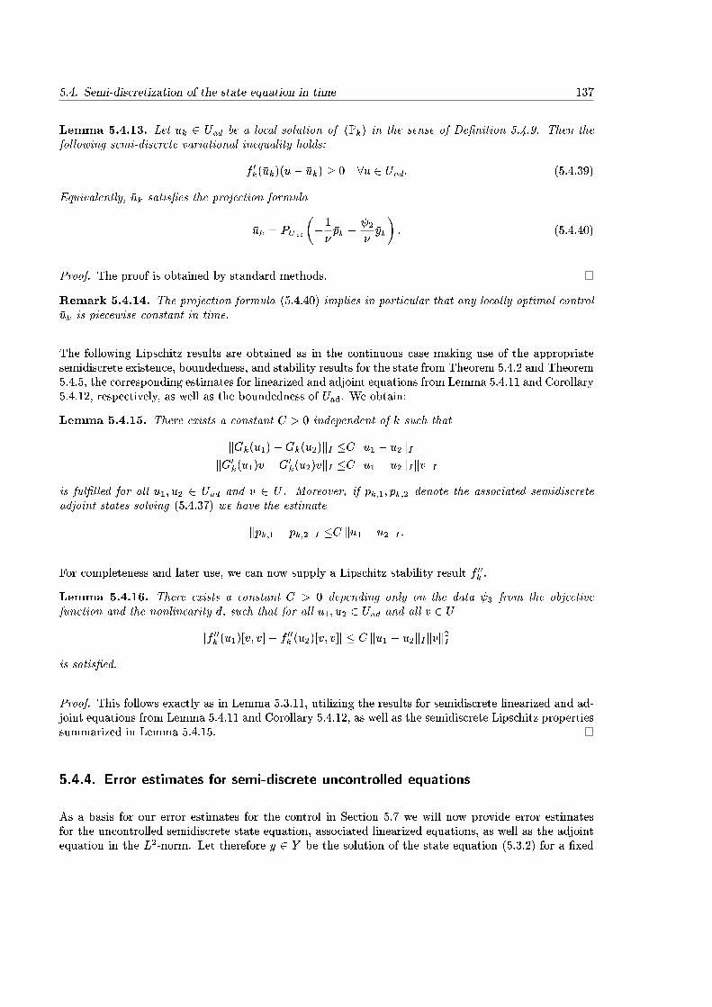
5.4. Semi-discretization of the state equation in time 137
Lemma 5.4.13. Let �uk 2 Uad be a local solution of (Pk) in the sense of De�nition 5.4.9. Then thefollowing semi-discrete variational inequality holds:
f 0k(�uk)(u� �uk) � 0 8u 2 Uad: (5.4.39)
Equivalently, �uk satis�es the projection formula
�uk = PUad
��1
��pk +
2��yk
�: (5.4.40)
Proof. The proof is obtained by standard methods.
Remark 5.4.14. The projection formula (5.4.40) implies in particular that any locally optimal control�uk is piecewise constant in time.
The following Lipschitz results are obtained as in the continuous case making use of the appropriatesemidiscrete existence, boundedness, and stability results for the state from Theorem 5.4.2 and Theorem5.4.5, the corresponding estimates for linearized and adjoint equations from Lemma 5.4.11 and Corollary5.4.12, respectively, as well as the boundedness of Uad. We obtain:
Lemma 5.4.15. There exists a constant C > 0 independent of k such that
kGk(u1)�Gk(u2)kI �C ku1 � u2kIkG0k(u1)v �G0k(u2)vkI �C ku1 � u2kIkvkI
is ful�lled for all u1; u2 2 Uad and v 2 U . Moreover, if pk;1; pk;2 denote the associated semidiscreteadjoint states solving (5.4.37) we have the estimate
kpk;1 � pk;2kI �C ku1 � u2kI :
For completeness and later use, we can now supply a Lipschitz stability result f 00k .
Lemma 5.4.16. There exists a constant C > 0 depending only on the data 3 from the objectivefunction and the nonlinearity d, such that for all u1; u2 2 Uad and all v 2 U
jf 00k (u1)[v; v]� f 00k (u2)[v; v]j � C ku1 � u2kIkvk2Iis satis�ed.
Proof. This follows exactly as in Lemma 5.3.11, utilizing the results for semidiscrete linearized and ad-joint equations from Lemma 5.4.11 and Corollary 5.4.12, as well as the semidiscrete Lipschitz propertiessummarized in Lemma 5.4.15.
5.4.4. Error estimates for semi-discrete uncontrolled equations
As a basis for our error estimates for the control in Section 5.7 we will now provide error estimatesfor the uncontrolled semidiscrete state equation, associated linearized equations, as well as the adjointequation in the L2-norm. Let therefore y 2 Y be the solution of the state equation (5.3.2) for a �xed
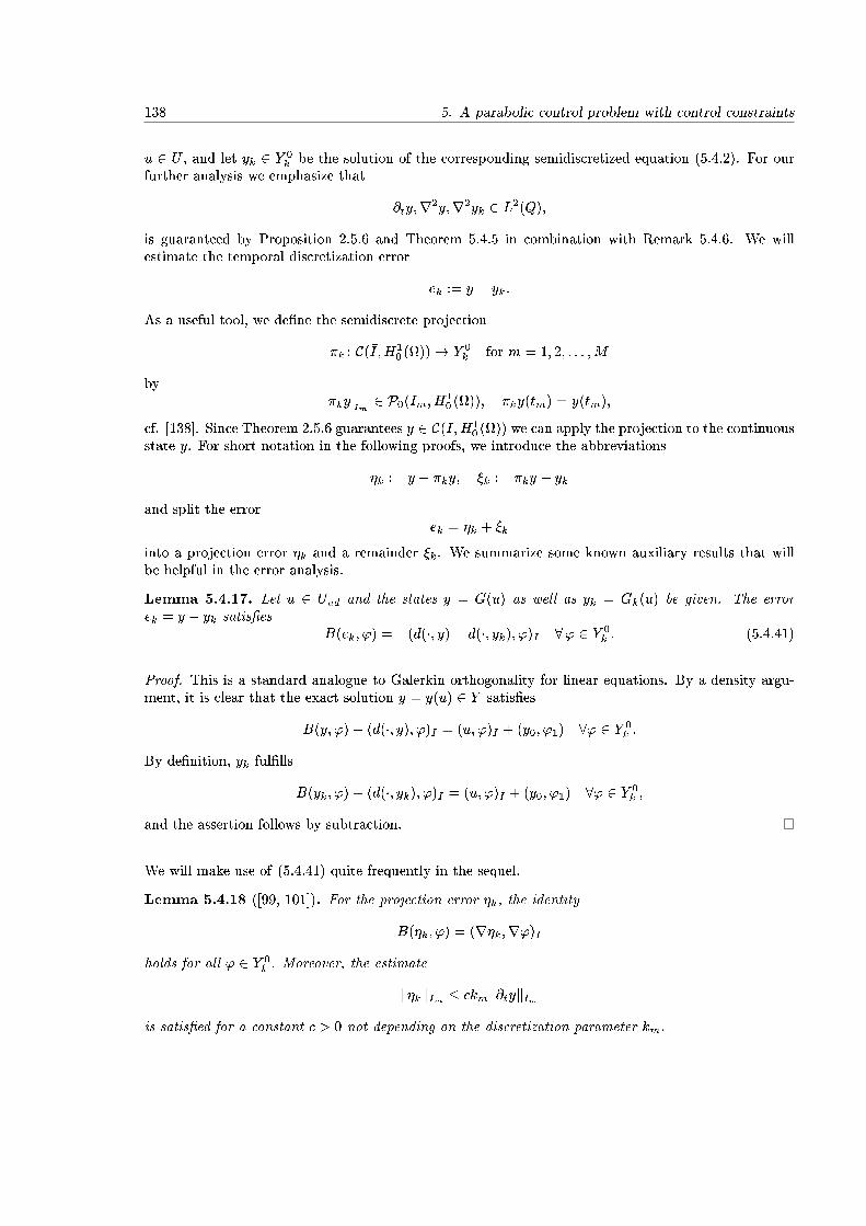
138 5. A parabolic control problem with control constraints
u 2 U , and let yk 2 Y 0k be the solution of the corresponding semidiscretized equation (5.4.2). For our
further analysis we emphasize that
@ty;r2y;r2yk 2 L2(Q);
is guaranteed by Proposition 2.5.6 and Theorem 5.4.5 in combination with Remark 5.4.6. We willestimate the temporal discretization error
ek := y � yk:
As a useful tool, we de�ne the semidiscrete projection
�k : C(�I;H10 ())! Y 0
k for m = 1; 2; : : : ;M
by�kyjIm 2 P0(Im; H
10 ()); �ky(tm) = y(tm);
cf. [138]. Since Theorem 2.5.6 guarantees y 2 C(�I;H10 ()) we can apply the projection to the continuous
state y. For short notation in the following proofs, we introduce the abbreviations
�k := y � �ky; �k := �ky � yk
and split the errorek = �k + �k
into a projection error �k and a remainder �k. We summarize some known auxiliary results that willbe helpful in the error analysis.
Lemma 5.4.17. Let u 2 Uad and the states y = G(u) as well as yk = Gk(u) be given. The errorek = y � yk satis�es
B(ek; ') = �(d(�; y)� d(�; yk); ')I 8' 2 Y 0k : (5.4.41)
Proof. This is a standard analogue to Galerkin orthogonality for linear equations. By a density argu-ment, it is clear that the exact solution y = y(u) 2 Y satis�es
B(y; ') + (d(�; y); ')I = (u; ')I + (y0; '1) 8' 2 Y 0k :
By de�nition, yk ful�lls
B(yk; ') + (d(�; yk); ')I = (u; ')I + (y0; '1) 8' 2 Y 0k ;
and the assertion follows by subtraction.
We will make use of (5.4.41) quite frequently in the sequel.
Lemma 5.4.18 ([99, 101]). For the projection error �k, the identity
B(�k; ') = (r�k;r')Iholds for all ' 2 Y 0
k . Moreover, the estimate
k�kkIm � ckmk@tykImis satis�ed for a constant c > 0 not depending on the discretization parameter km.

5.4. Semi-discretization of the state equation in time 139
Proof. The �rst identity follows from straight-forward calculations utilizing the properties of �k. Theprojection error estimate is a conclusion from the Bramble-Hilbert Lemma, cf. [138].
Lemma 5.4.19. For all v 2 Y 0k , the following estimate is satis�ed:
kvk21;2 + krvk2I � B(v; v):
Proof. We refer to the proof of Lemma 5.7 in [101], where an estimate for the term krvk2I was shown,which was su�cient for the linear setting. We follow these steps and add
B(v; v) = (rv;rv)I +M�1Xm=1
([v]m; v+m) + (v+0 ; v
+0 ) (5.4.42)
B(v; v) = (rv;rv)I +M�1Xm=1
(�v�m; [v]m) + (v�M ; v�M ) (5.4.43)
which is valid for v 2 Y 0k , cf. (5.4.5) on page 128. We obtain
B(v; v) = krvk2I +1
2
M�1Xm=1
k[v]mk2 + kv+0 k2 + kv�Mk2!;
since v+m � v�m = [vm]. Now, the assertion is obtained similar to the proof of Theorem 5.4.5.
The error estimate due to time-discretization of the state equation is now obtained following ideas thatare known for elliptic problems, cf. [23].
Theorem 5.4.20. For the error ek := y� yk between the continuous solution y 2 Y of (5.3.2) and thedG(0) semidiscretized solution yk 2 Y 0
k of (5.4.2) the estimate
kekkI � Ckk@tykIholds with a constant C that is independent of the size of the time steps k.
Proof. As in [23] for elliptic problems, we introduce a function ~d de�ned by
~d(t; x) =
(d(t;x;y(t;x))�d(t;x;yk(t;x))
y(t;x)�yk(t;x)if y(t; x) 6= yk(t; x)
0 else.
Note that k ~dk1;1 � c for a c > 0 due to the boundedness of Uad, the uniform boundedness of thestates y and yk, and the Lipschitz continuity of d. Then, we use known duality arguments and de�ne~pk 2 Y 0
k to be the solution of the auxiliary dual equation
B('; ~pk) + ('; ~d~pk)I = ('; ek)I 8 ' 2 Y 0k : (5.4.44)
Testing (5.4.44) with ' = �k 2 Y 0k yields
(�k; ek)I = B(�k; ~pk) + (�k; ~d~pk)I = B(ek; ~pk)�B(�k; ~pk) + (ek � �k; ~d~pk)I : (5.4.45)
To this, we apply (5.4.41) from Lemma 5.4.17 and arrive at
(�k; ek)I = �B(�k; ~pk)� (d(�; y)� d(�; yk); ~pk)I + (ek; ~d~pk)I � (�k; ~d~pk)I : (5.4.46)
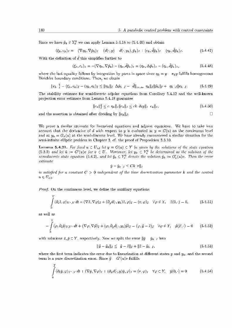
140 5. A parabolic control problem with control constraints
Since we have ~pk 2 Y 0k we can apply Lemma 5.4.18 to (5.4.46) and obtain
(�k; ek)I = �(r�k;r~pk)I � (d(�; y)� d(�; yk); ~pk)I + (ek; ~d~pk)I � (�k; ~d~pk)I : (5.4.47)
With the de�nition of ~d this simpli�es further to
(�k; ek)I = �(r�k;r~pk)� (�k; ~d~pk)I = (�k;�~pk)I � (�k; ~d~pk)I ; (5.4.48)
where the last equality follows by integration by parts in space since �k = y� �ky ful�lls homogeneousDirichlet boundary conditions. Then, we obtain
kekk2I = (�k; ek)I + (�k; ek)I � k�kkIk�~pkkI + k ~dk1;1k�kkIk~pkkI + k�kkIkekkI : (5.4.49)
The stability estimate for semidiscrete adjoint equations from Corollary 5.4.12 and the well-knownprojection error estimate from Lemma 5.4.18 guarantee
kekk2I � ck�kkIkekkI � ckk@tykIkekkI ; (5.4.50)
and the assertion is obtained after dividing by kekkI .
We prove a similar estimate for linearized equations and adjoint equations. We have to take intoaccount that the derivative of d with respect to y is evaluated at y = G(u) on the continuous leveland at yk = Gk(u) at the semi-discrete level. We have already encountered a similar situation for thesemi-in�nite elliptic problem in Chapter 3, cf. the proof of Proposition 3.3.10.
Lemma 5.4.21. For �xed u 2 Uad let y = G(u) 2 Y be given by the solutions of the state equation(5.3.2) and let ~u := G0(u)v for v 2 U . Moreover, let yk 2 Y 0
k be determined as the solution of thesemidiscrete state equation (5.4.2), and let ~yk 2 Y 0
k denote the solution ~yk := G0k(u)v. Then the errorestimate
k~y � ~ykkI � CkkvkIis satis�ed for a constant C > 0 independent of the time discretization parameter k and the controlu 2 Uad.
Proof. On the continuous level, we de�ne the auxiliary equations
TZ0
h@t~z; 'iV �;V dt+ (r~z;r')I + (@yd(�; yk)~z; ')I = (v; ')I 8' 2 Y; ~z(0; �) = 0; (5.4.51)
as well as
�TZ0
h'; @t~piV;V � dt+ (r';r~p)I + ('; @yd(�; yk)~p)I = ('; ~y � ~z)I 8' 2 Y; ~p(T; �) = 0 (5.4.52)
with solutions ~z; ~p 2 Y , respectively. Now we split the error k~y � ~ykkI intok~y � ~ykkI � k~y � ~zkI + k~z � ~ykkI ; (5.4.53)
where the �rst term indicates the error due to linearization at di�erent states y and yk, and the secondterm is a pure discretization error. Since ~y = G0(u)v ful�lls
TZ0
h@t~y; 'iV �;V dt+ (r~y;r')I + (@yd(�; y)~y; ')I = (v; ')I 8' 2 Y; ~y(0; �) = 0 (5.4.54)
5.4. Semi-discretization of the state equation in time 141
with y = G(u) we obtain for the �rst term in (5.4.53) that
TR0
h@t(~y � ~z); 'iV �;V + (r(~y � ~z);r')I + (@yd(�; y)(~y � ~z); ')I = ((@yd(�; yk)� @yd(�; y))~z; ')I ;(~y � ~z)(0; �) = 0
(5.4.55)is satis�ed for all ' 2 Y . Testing (5.4.52) with ' = ~y � ~z and integration by parts in time yields
k~y � ~zk2I = �TR0
h~y � ~z; @t~piV;V � dt+ (r(~y � ~z);r~p)I + (~y � ~z; @yd(�; yk)~p)I
=TR0
h@t(~y � ~z); ~piV �;V dt+ (r(~y � ~z);r~p)I + (~y � ~z; @yd(�; yk)~p)I :(5.4.56)
On the other hand, testing (5.4.55) with ' = ~p leads to
TZ0
h@t(~y� ~z); ~piV �;V dt+(r(~y� ~z);r~p)I+(@yd(�; y)(~y� ~z); ~p)I = ((@yd(�; yk)�@yd(�; y))~z; ~p)I : (5.4.57)
Combining (5.4.56) and (5.4.57) yields
k~y � ~zk2I = �(@yd(�; y)(~y � ~z); ~p)I + ((@yd(�; yk)� @yd(�; y))~z; ~p)I + (~y � ~z; @yd(�; yk)~p)I ; (5.4.58)
which simpli�es tok~y � ~zk2I = ((@yd(�; yk)� @yd(�; y)) ~y; ~p)I : (5.4.59)
This can be estimated as
k~y � ~zk2I � k@yd(�; yk)� @yd(�; y)kIk~ykL4(Q)k~pkL4(Q); (5.4.60)
and by the embedding L1(I; V ) ,! L4(Q) and the Lipschitz continuity of @yd as well as the boundednessof Uad we arrive at
k~y � ~zk2I � c ky � ykkIk~ykL1(I;V )k~pkL1(I;V ):
The error estimate for the states from Theorem 5.4.20 as well as the stability estimates for linearizedand adjoint equations from Propositions 2.5.2 and 2.5.7 deliver the estimate
k~y � ~zkI � ckk@tykIkvkI ;and using Theorem 2.5.6 to estimate k@tykI we obtain
k~y � ~zkI � ckkvkIby the boundedness of Uad. To estimate the second term in (5.4.53), we can apply the discretizationerror estimates from [101] with only minor adaptation due to the term @yd(�; yk(u)), where again yk isuniformly bounded independent of the discretization parameter. Alternatively, the discretization errorestimate for semilinear equations from Theorem 5.4.20 can be applied.
It remains to estimate the error for the adjoint equation.
Lemma 5.4.22. For �xed u 2 Uad let y 2 Y and p 2 Y be given by the solutions of the state equation(5.3.2) and the adjoint equation (5.3.5), respectively. Moreover, let yk 2 Y 0
k and pk 2 Y 0k be determined
as solutions of the semidiscrete state equation (5.4.2) and adjoint equation (5.4.37). Then the errorestimate
kp� pkkI � Ck (k@tykI + k@tpkI)is satis�ed for a constant C > 0 independent of the time discretization parameter k and independent ofu 2 Uad.
142 5. A parabolic control problem with control constraints
Proof. The proof is similar to the one of Lemma 5.4.21, introducing an auxiliary adjoint state p 2 Y ,de�ned as the solution of
�TZ0
h'; @tpiV;V � dt+ (r';rp)I + ('; @yd(�; yk(u))p)I = ('; 1yk + 2u+ 3)I 8' 2 Y;
p(T; �) = 0:
We split the error intokp� pkkI � kp� pkI + kp� pkkI :
The term kp � pkI can be estimated with similar steps as in the proof of Lemma 5.4.21, making useof Theorem 5.4.20, Proposition 2.5.7, and the boundedness of Uad. We also refer to [118] for furtherdetails. The second term to estimate is again a pure discretization error and accounts for the termk@tpk. This is obtained with arguments similar to [101].
5.4.5. Semidiscrete coercivity
Before discussing the spatial discretization of the state equation we state a semidiscrete analogue toCorollary 5.3.13. We prove a coercivity result for f 00k in the neighborhood of �u, which will later beextended to a coercivity result in the neighborhood of a local semidiscrete solution �uk approximating�u.
Lemma 5.4.23. Let �u be a local solution of (P) and let Assumptions 5.3.1 and 5.3.9 be valid. Thenthere exists an " > 0, such that for all u 2 Uad with ku� �ukI � " and all v 2 L1(Q)
f 00k (u)[v; v] ��
4kvk2I
holds for k su�ciently small.
Proof. With the de�nition of f 00 and f 00k we obtain
jf 00k (u)[v; v]� f 00(u)[v; v]j �ZZQ
��p@yyd(�; y)~y2 � pk@yyd(�; yk)~y2k�� dxdt
+
ZZQ
�� 1(~y2k � ~y2) + 2 2v(~yk � ~y)�� dxdt
�ZZQ
j( 1(~yk + ~y) + 2 2v)(~yk � ~y)j dxdt
+
ZZQ
��(p� pk)@yyd(�; y)~y2�� dxdt
+
ZZQ
jpk@yyd(�; y)(~y � ~yk)(~yk + ~y)j dxdt
+
ZZQ
��pk(@yyd(�; y)� @yyd(�; yk))~y2k�� dxdt;
5.5. Discretization of the state equation in space 143
similar to Lemma 5.3.11. The following steps are completely analogous to the proof of Lemma 5.4.16,making use of semidiscrete stability and discretization error estimates. Estimating the integrals byH�older's inequality yields
jf 00k (u)[v; v]� f 00(u)[v; v]j � c(k~ykkI + k~ykI + kvkI)k~yk � ~ykI+c k@yyd(�; yk)k1;1kpk � pkIk~yk2L4(Q))
+c kpkk1;1k@yyd(�; y)k1;1(k~ykkI + k~ykI)k~yk � ~ykI+ckpkk1;1kyk � ykIk~ykk2L4(Q):
In the last line, we have used the uniform boundedness of y as well as yk and pk independent of k andu as well as the Lipschitz continuity of @yyd. By the embedding
L1(I;H10 ()) ,! L4(Q);
Proposition 2.5.2 and estimates (5.4.34) and (5.4.36) yield
k~ykL4(Q) � c kvkI ; k~ykkL4(Q) � c kvkI ;
as well as
k~ykI � c kvkI ; k~ykkI � c kvkI :Then, the boundedness of Uad and @yyd as well as yk; pk; ~yk yield
jf 00k (u)[v; v]� f 00(u)[v; v]j � ck~yk � ~ykIkvkI + c kpk � pkIkvk2I + ckyk � ykIkvk2I : (5.4.61)
Now, the discretization error estimates
ky � ykkI + kp� pkkI � c k; k~y � ~ykkI � c kkvkI
from Theorem 5.4.20 and Lemmas 5.4.21 and 5.4.22 lead to
jf 00k (u)[v; v]� f 00(u)[v; v]j � c kkvk2I :
Since this tends to zero as k tends to zero, the assertion is obtained by Corollary 5.3.13, observing that
f 00k (u)[v; v] = f 00(u)[v; v] + f 00k (u)[v; v]� f 00(u)[v; v] � �
2kvk2I � ckkvk2I :
5.5. Discretization of the state equation in space
On the second level of discretization we discretize the state equation in space. Here, we use usualconforming �nite elements. We proceed similar to the last section. After a brief introduction to thediscretization, we will basically discuss the same steps as before. Special emphasis will be placed on aboundedness result for discrete solutions of the state equation, and on error estimates for uncontrolledequations due to the spatial discretization.
144 5. A parabolic control problem with control constraints
5.5.1. Preliminaries
Following the lines of [102], we consider here two-dimensional shape regular meshes consisting ofnonoverlapping quadrilateral cells K. We refer to e. g., [34] for the de�nition of regular meshes. Wedenote the mesh by Th = fKg and de�ne the discretization parameter h : ! R as a cellwise constantfunction by setting hjK = hK with the diameter hK of the cell K. We use the symbol h also for themaximal cell size, i. e.,
h = maxhK :
We bene�t from the fact that is polygonally bounded.
On the mesh Th we construct a conforming �nite element space Vh � H10 () in a standard way. Note
that in contrast to Chapter 3 the use of quadrilateral cells instead of triangles makes it necessary toconsider bilinear functions. We de�ne the discrete space
Vh = fv 2 H10 ()jvjK 2 Q1(K) for K 2 Thg;
where Q1(K) consists of shape functions obtained via bilinear transformations of polynomials in cQ1(K)de�ned on the reference cell K = (0; 1)2; cf. also Section 3.2 in [101]. Then, we utilize the space-time�nite element space
Y 0;1k;h = fvkh 2 L2(I; Vh)jvkhjIm 2 P0(Im; Vh); m = 1; 2; : : : ;Mg � Y 0
k :
The so-called cG(1)dG(0) discretization of the state equation for given control u 2 U has the followingform:
Find a state ykh = ykh(u) 2 Y 0;1k;h such that
B(ykh; ') + (d(�; ykh); ')I = (u; ')I + (y0; '1) 8' 2 Y 0;1k;h : (5.5.1)
5.5.2. Existence results and stability estimates for the discrete state equation
We are �rst concerned with the existence of a solution ykh of the fully discrete state equation for allu 2 U and y0 2 H1
0 ().
Theorem 5.5.1. Let Assumption 5.2.1 be satis�ed. Then, for each u 2 U and y0 2 H10 () \ L1(),
there exists a unique solution ykh 2 Y 0;1k;h \ L1(Q) of equation (5.5.1).
Proof. The existence of ykh is a consequence of Brouwer's �xed point theorem using the monotonicityand Lipschitz continuity of d; we refer to Appendix A.1 for more details. The uniqueness follows fromthe monotonicity of d with respect to y by assumption of the contrary.
In a second step, we will again need to supply a boundedness result for ykh that is independent of the dis-cretization parameters. Noting that error estimates for the semidiscrete equations in the L1(I; L2())-norm appeared in a quite natural way, it is now promising to obtain boundedness of the discretesolutions by an inverse estimate between the norms on L1() and L2(). In fact, a direct extension ofStampacchia's method to spatially discrete problems is not possible, since test functions vkh = ykh � bare not generally functions in Y 0;1
k;h . By means of the spatial L2-projection
�h : H10 ()! Vh
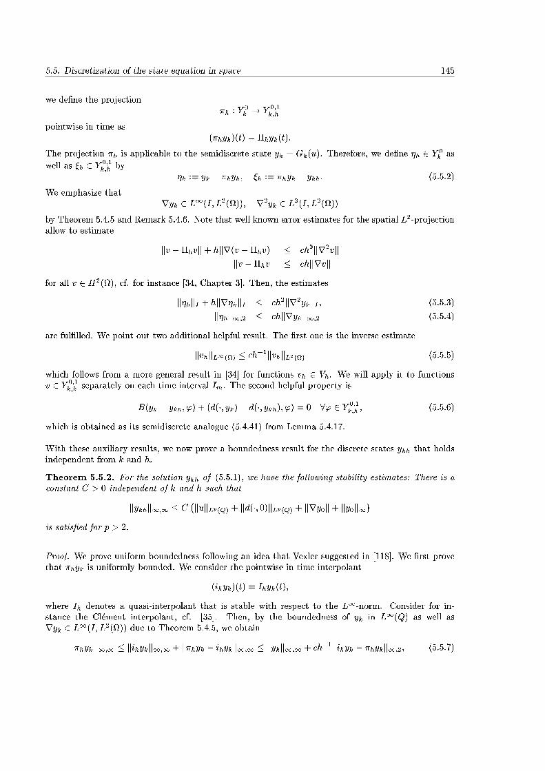
5.5. Discretization of the state equation in space 145
we de�ne the projection�h : Y
0k ! Y 0;1
k;h
pointwise in time as(�hyk)(t) = �hyk(t):
The projection �h is applicable to the semidiscrete state yk = Gk(u). Therefore, we de�ne �h 2 Y 0k as
well as �h 2 Y 0;1k;h by
�h := yk � �hyk; �h := �hyk � ykh: (5.5.2)
We emphasize thatryk 2 L1(I; L2()); r2yk 2 L2(I; L2())
by Theorem 5.4.5 and Remark 5.4.6. Note that well known error estimates for the spatial L2-projectionallow to estimate
kv ��hvk+ hkr(v ��hv)k � ch2kr2vkkv ��hvk � chkrvk
for all v 2 H2(), cf. for instance [34, Chapter 3]. Then, the estimates
k�hkI + hkr�hkI � ch2kr2ykkI ; (5.5.3)
k�hk1;2 � chkrykk1;2 (5.5.4)
are ful�lled. We point out two additional helpful result. The �rst one is the inverse estimate
kvhkL1() � ch�1kvhkL2() (5.5.5)
which follows from a more general result in [34] for functions vh 2 Vh. We will apply it to functionsv 2 Y 0;1
k;h separately on each time interval Im. The second helpful property is
B(yk � ykh; ') + (d(�; yk)� d(�; ykh); ') = 0 8' 2 Y 0;1k;h ; (5.5.6)
which is obtained as its semidiscrete analogue (5.4.41) from Lemma 5.4.17.
With these auxiliary results, we now prove a boundedness result for the discrete states ykh that holdsindependent from k and h.
Theorem 5.5.2. For the solution ykh of (5.5.1), we have the following stability estimates: There is aconstant C > 0 independent of k and h such that
kykhk1;1 � C�kukLp(Q) + kd(�; 0)kLp(Q) + kry0k+ ky0k1
�is satis�ed for p > 2.
Proof. We prove uniform boundedness following an idea that Vexler suggested in [118]. We �rst provethat �hyk is uniformly bounded. We consider the pointwise in time interpolant
(ihyk)(t) = Ihyk(t);
where Ih denotes a quasi-interpolant that is stable with respect to the L1-norm. Consider for in-stance the Cl�ement interpolant, cf. [35]. Then, by the boundedness of yk in L1(Q) as well asryk 2 L1(I; L2()) due to Theorem 5.4.5, we obtain
k�hykk1;1 � kihykk1;1 + k�hyk � ihykk1;1 � kykk1;1 + ch�1kihyk � �hykk1;2; (5.5.7)
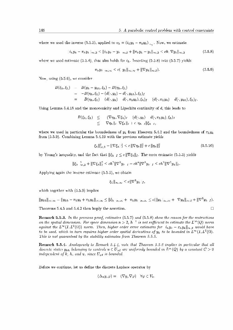
146 5. A parabolic control problem with control constraints
where we used the inverse (5.5.5), applied to vh = (ihyk � �hyk)jIm . Now, we estimate
kihyk � �hykk1;2 � kihyk � ykk1;2 + k�hyk � ykk1;2 � chkrykk1;2 (5.5.8)
where we used estimate (5.5.4), that also holds for ih. Inserting (5.5.8) into (5.5.7) yields
k�hykk1;1 � c(kykk1;1 + krykk1;2): (5.5.9)
Now, using (5.5.6), we consider
B(�h; �h) = B(yk � ykh; �h)�B(�h; �h)
= �B(�h; �h)� (d(�; yk)� d(�; ykh); �h)I= �B(�h; �h)� (d(�; yk)� d(�; �hyk); �h)I � (d(�; �hyk)� d(�; ykh); �h)I :
Using Lemma 5.4.18 and the monotonicity and Lipschitz continuity of d, this leads to
B(�h; �h) � �(r�h;r�h)I � (d(�; yk)� d(�; �hyk); �h)I� kr�hkIkr�hkI + ck�hkIk�hkI ;
where we used in particular the boundedness of yk from Theorem 5.4.2 and the boundedness of �hykfrom (5.5.9). Combining Lemma 5.4.19 with the previous estimate yields
k�hk21;2 + kr�hk2I � c kr�hk2I + c k�hk2I (5.5.10)
by Young's inequality, and the fact that k�hkI � c kr�hkI . The error estimate (5.5.3) yields
k�hk21;2 + kr�hk2I � ch2kr2ykkI + ch4kr2ykkI � ch2kr2ykkI :
Applying again the inverse estimate (5.5.5), we obtain
k�hk1;1 � ckr2ykkI ;
which together with (5.5.9) implies
kykhk1;1 = kykh � �hyk + �hykk1;1 � k�hk1;1 + k�hykk1;1 � c(kykk1;1 + krykk1;2 + kr2ykkI):
Theorems 5.4.5 and 5.4.2 then imply the assertion.
Remark 5.5.3. In the previous proof, estimates (5.5.7) and (5.5.8) show the reason for the restrictionson the spatial dimension. For space dimension n > 2, h�1 is not su�cient to estimate the L1(Q) normagainst the L1(I; L2()) norm. Then, higher order error estimates for kihyk � �hykk1;2 would haveto be used, which in turn requires higher order spatial derivatives of yk to be bounded in L1(I; L2().This is not guaranteed by the stability estimates from Theorem 5.5.5.
Remark 5.5.4. Analogously to Remark 5.4.4, note that Theorem 5.5.2 implies in particular that alldiscrete states ykh belonging to controls u 2 Uad are uniformly bounded in L1(Q) by a constant C > 0independent of k, h, and u, since Uad is bounded.
Before we continue, let us de�ne the discrete Laplace operator by
(�hy; ') = �(ry;r') 8' 2 Vh:
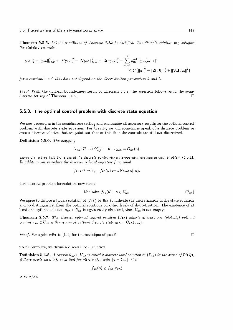
5.5. Discretization of the state equation in space 147
Theorem 5.5.5. Let the conditions of Theorem 5.5.2 be satis�ed. The discrete solution ykh satis�esthe stability estimate
kykhk2I + kykhk21;2 + krykhk2I + krykhk21;2 + k�hykhk2I +MXm=1
k�1m k[ykh]m�1k2
� C�kuk2I + kd(�; 0)k2I + kr�hy0k2
�for a constant c > 0 that does not depend on the discretization parameters k and h.
Proof. With the uniform boundedness result of Theorem 5.5.2, the assertion follows as in the semi-discrete setting of Theorem 5.4.5.
5.5.3. The optimal control problem with discrete state equation
We now proceed as in the semidiscrete setting and summarize all necessary results for the optimal controlproblem with discrete state equation. For brevity, we will sometimes speak of a discrete problem oreven a discrete solution, but we point out that at this time the controls are still not discretized.
De�nition 5.5.6. The mapping
Gkh : U ! \Y 0;1k;h ; u 7! ykh = Gkh(u);
where ykh solves (5.5.1), is called the discrete control-to-state-operator associated with Problem (5.3.1).In addition, we introduce the discrete reduced objective functional
fkh : U ! R; fkh(u) := J(Gkh(u); u):
The discrete problem formulation now reads
Minimize fkh(u) u 2 Uad: (Pkh)
We agree to denote a (local) solution of (Pkh) by �ukh to indicate the discretization of the state equationand to distinguish it from the optimal solutions on other levels of discretization. The existence of atleast one optimal solution �ukh 2 Uad is again easily obtained, since Uad is not empty.
Theorem 5.5.7. The discrete optimal control problem (Pkh) admits at least one (globally) optimalcontrol �ukh 2 Uad with associated optimal discrete state �ykh = Gkh(�ukh).
Proof. We again refer to [144] for the technique of proof.
To be complete, we de�ne a discrete local solution.
De�nition 5.5.8. A control �ukh 2 Uad is called a discrete local solution to (Pkh) in the sense of L2(Q),if there exists an " > 0 such that for all u 2 Uad with ku� �ukhkI � "
fkh(u) � fkh(�ukh)
is satis�ed.
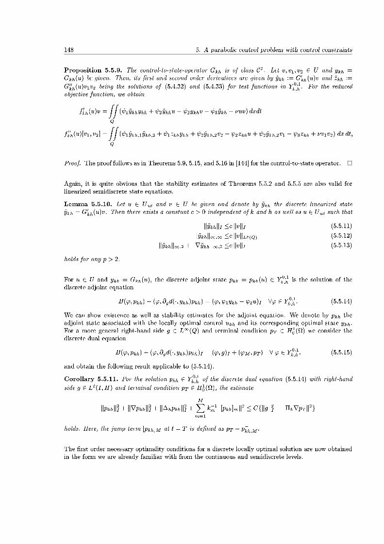
148 5. A parabolic control problem with control constraints
Proposition 5.5.9. The control-to-state-operator Gkh is of class C2. Let v; v1; v2 2 U and ykh =Gkh(u) be given. Then, its �rst and second order derivatives are given by ~ykh := G0kh(u)v and ~zkh :=
G00kh(u)v1v2 being the solutions of (5.4.32) and (5.4.33) for test functions in Y 0;1k;h . For the reduced
objective function, we obtain
f 0kh(u)v =
ZZQ
( 1~ykhykh + 2~ykhu+ 2ykhv + 3~ykh + �uv) dxdt
f 00kh(u)[v1; v2] =
ZZQ
( 1~ykh;1~ykh;2 + 1zkhykh + 2~ykh;2v2 + 2zkhu+ 2~ykh;2v1 + 3zkh + �v1v2) dx dt;
Proof. The proof follows as in Theorems 5.9, 5.15, and 5.16 in [144] for the control-to-state operator.
Again, it is quite obvious that the stability estimates of Theorems 5.5.2 and 5.5.5 are also valid forlinearized semidiscrete state equations.
Lemma 5.5.10. Let u 2 Uad and v 2 U be given and denote by ~ykh the discrete linearized state~ykh = G0kh(u)v. Then there exists a constant c > 0 independent of k and h as well as u 2 Uad such that
k~ykhkI �c kvkI (5.5.11)
k~ykhk1;1 �c kvkLp(Q) (5.5.12)
k~ykhk1;2 + kr~ykhk1;2 �c kvkI (5.5.13)
holds for any p > 2.
For u 2 U and ykh = Gkh(u), the discrete adjoint state pkh = pkh(u) 2 Y 0;1k;h is the solution of the
discrete adjoint equation
B('; pkh) + ('; @yd(�; ykh)pkh) = ('; 1ykh + 2u)I 8' 2 Y 0;1k;h : (5.5.14)
We can show existence as well as stability estimates for the adjoint equation. We denote by �pkh theadjoint state associated with the locally optimal control �ukh and its corresponding optimal state �ykh.For a more general right-hand side g 2 L1(Q) and terminal condition pT 2 H1
0 () we consider thediscrete dual equation
B('; pkh) + ('; @yd(�; ykh)pkh)I = ('; g)I + ('M ; pT ) 8 ' 2 Y 0;1k;h : (5.5.15)
and obtain the following result applicable to (5.5.14).
Corollary 5.5.11. For the solution pkh 2 Y 0;1k;h of the discrete dual equation (5.5.14) with right-hand
side g 2 L2(I;H) and terminal condition pT 2 H10 (), the estimate
kpkhk2I + krpkhk2I + k�hpkhk2I +MXm=1
k�1m k[pkh]mk2 � Cfkgk2I + k�hrpT k2g
holds. Here, the jump term [pkh]M at t = T is de�ned as pT � p�kh;M .
The �rst order necessary optimality conditions for a discrete locally optimal solution are now obtainedin the form we are already familiar with from the continuous and semidiscrete levels.
5.5. Discretization of the state equation in space 149
Lemma 5.5.12. Let �ukh 2 Uad be a local solution of (Pkh) in the sense of De�nition 5.5.8. Then thefollowing discrete variational inequality holds:
f 0kh(�ukh)(u� �ukh) � 0 8u 2 Uad; (5.5.16)
Equivalently, �ukh satis�es the projection formula
�ukh = PUad
��1
��pkh +
2��ykh
�: (5.5.17)
Proof. The proof is standard, we refer, again e. g., to [144].
We infer that �ukh is piecewise constant in time, but not necessarily cellwise bilinear in space.
For future reference, let us also state a Lipschitz continuity result for Gkh and its derivatives, whichcan be shown as in the semidiscrete setting of Lemma 5.4.15.
Lemma 5.5.13. Let u1; u2 2 Uad and v 2 U be given. Then there exists a constant C > 0 independentof k and h such that
kGkh(u1)�Gkh(u2)kI �C ku1 � u2kIkG0kh(u1)v �G0kh(u2)vkI �C ku1 � u2kIkvkI
is ful�lled.
The following Lipschitz result for the discrete objective function is equally straight-forward to prove.
Lemma 5.5.14. The �rst derivative of fkh ful�lls a Lipschitz condition, i. e. there exists a constantC > 0 such that for all u1; u2 2 Uad and all v 2 U
jf 0kh(u1)v � f 0kh(u2)vj � C ku1 � u2kIkvkIis satis�ed.
Proof. This follows in a straight-forward manner, making use of Lipschitz results for the state andlinearized state equation from Lemma 5.5.13.
5.5.4. Error estimates for discrete uncontrolled equations
We now prove error estimates for the uncontrolled discrete state and adjoint equations in the L2-norm.Analogously to the semidiscrete level, we de�ne the error eh due to spatial discretization by
eh := yk � ykh;
and again decompose it into a projection error and a remainder, term, i.e.
eh = �h + �h;
150 5. A parabolic control problem with control constraints
where �h and �h are de�ne in (5.5.2) on page 145. Again, we follow [23]. We de�ne pk 2 Y 0k as the
solution of the auxiliary semidiscrete dual equation
B('; pk) + ('; dpk)I = ('; eh)I 8 ' 2 Y 0k ; (5.5.18)
with
d(t; x) =
(d(t;x;yk(t;x))�d(t;x;ykh(t;x))
yk(t;x)�ykh(t;x)if yk(t; x) 6= ykh(t; x)
0 else.
In addition to the abbreviations �h and �h we introduce the short notation
��h := pk � �hpk:
and make use of the statements
B(�h; ��h) =(r�h;r��h); (5.5.19)
B(�h; ��h) �kr�hkIkr��hkI + c k�hkIkehkI ; (5.5.20)
that have been proven in [101, Lemmas 5.7, 5.8] by direct calculations. Our main error estimate for thediscrete state equation is now easily obtained.
Theorem 5.5.15. For the error eh := yk � ykh between the dG(0) semidiscretized solution yk 2 Y 0k of
(5.4.2) and the fully cG(1)dG(0) discretized solution ykh 2 Y 0;1k;h of (5.5.1), we have the error estimate
kehkI � Ch2kr2ykkI ;
where the constant C is independent of the mesh size h and the size of the time steps k.
Proof. Testing (5.5.18) with ' = eh 2 Y 0k yields
kehk2I =B(eh; pk) + (eh; dpk)I
=B(eh; pk � �hpk) +B(eh; �hpk) + (eh; d(pk � �hpk))I + (eh; d�hpk)
=B(eh; ��h) +B(eh; �hpk) + (eh; d�
�h) + (eh; d�hpk)
=B(eh; ��h)� (d(�; yk)� d(�; ykh); �hpk) + (eh; d�
�h) + (eh; d�hpk);
where the last equality follows from (5.5.6) by the fact that �hpk 2 Y 0;1k;h . With the de�nition of d, this
simpli�es further to
kehk2I = B(eh; ��h) + (eh; d�
�h)I = B(�h; �
�h) +B(�h; �
�h) + (eh; d�
�h)I : (5.5.21)
With (5.5.19) and (5.5.20) we estimate (5.5.21) by
kehk2I � kr�hkIkr��hkI + kr�hkIkr��hkI + c k�hkIkehkI + c k�hkIk��hkI + c k�hkIk��hkI (5.5.22)
since yk, ykh, and d are bounded in L1(Q). From Lemma 5.4.19 we also know that
kr�hk2I + k�hk2I � B(�h; �h):
In the proof of Theorem 5.5.2, we have estimated B(�h; �h) against projection error estimates, cf.(5.5.10), and we obtain
kr�hk2I + k�hk2I � c�kr�hk2I + k�hk2I
�:
5.5. Discretization of the state equation in space 151
Inserting this in (5.5.22), we obtain
kehk2I � c(kr�hkIkr��hkI + k�hkIkr��hkI + kr�hkIk��hkI + k�hkIk��hkI + k�hkIkehkI): (5.5.23)
Now observe that analogously to the error estimates (5.5.3) we have
k��hkI � ch2kr2pkkI ; kr��hkI � chkr2pkkI :Applying this and the error estimate (5.5.3) to (5.5.23) leads to
kehk2I � ch2kr2pkkIkr2ykkI + ch2kr2ykkIkehkI :Now, with the same arguments as in Remark 5.4.6, we have
kr2pkkI � c k�pkkI � c kehkI ;due to Corollary 5.4.12, which inserted into (5.5.23) yields the assertion.
As on the semidiscrete discretization level in Section 5.4.4 we also obtain error estimates for linearizedstates and adjoint states. We state them without proof.
Lemma 5.5.16. For u 2 Uad let yk 2 Y 0k be given by the solutions of the semidiscrete state equation
(5.4.2) and and let ~yk := G0k(u)v 2 Y 0k be the solution of the linearized state equation, respectively.
Moreover, let ykh 2 Y 0;1k;h and ~ykh := G0kh(u)v 2 Y 0;1
k;h denote the solutions of the discrete state equation(5.5.1) and a corresponding linearized equation. Then the error estimate
k~yk � ~ykhkI � Ch2kvkIis satis�ed for a constant C > 0 independent of the space discretization.
Lemma 5.5.17. For u 2 Uad let yk 2 Y 0k and pk 2 Y 0
k be given by the solutions of the semidiscrete state
equation (5.4.2) and adjoint equation (5.4.37), respectively. Moreover, let ykh 2 Y 0;1k;h and pkh 2 Y 0;1
k;h
denote the solutions of the discrete state equation (5.5.1) and adjoint equation (5.5.14). Then the errorestimate
kpk � pkhkI � Ch2�kr2ykkI + kr2pkkI
�is satis�ed for a constant C > 0 independent of the space discretization.
Finally, we prove an auxiliary discretization error estimate for the objective function.
Lemma 5.5.18. Let u 2 Uad and v 2 U be given. Then the estimate
jf 0k(u)v � f 0kh(u)vj � Ch2kvkIholds with a constant C > 0 independent of h.
Proof. With yk := Gk(u), ykh := Gkh(u), as well as ~yk := G0k(u)v and ~ykh := G0kh(u)v, direct calcula-tions imply
jf 0k(u)v � f 0kh(u)vj =j ( 1(yk � ykh); ~yk)I + ( 1(~yk � ~ykh); ykh)I + ( 2(~yk � ~ykh); u)I + ( 2(yk � ykh); v)I j�ck~ykh � ~ykkI + c kykh � ykkI
by the boundedness of Uad, the boundedness results of Theorem 5.5.2 and estimate (5.4.35). The errorestimates from Theorem 5.5.15 and Lemma 5.5.16 yield the assertion.
We will also need coercivity results of the second derivative of fkh, but only in the neighborhood ofa semi-discrete optimal solution �uk that has to correspond to a local solution �u on the continuouslevel. We therefore postpone the desired estimates until we prove error estimates for locally optimalcontrols.
152 5. A parabolic control problem with control constraints
5.6. Control discretization
The third level of discretization involves the discretization of the controls, if desired. We introduce asubspace U� � U , where the subscript � indicates control discretization in one of several possible waysto be discussed below. A discrete version of (P) then reads
Minimize fkh(u�); subject to u� 2 Uad \ U�; (P�)
where the subscript � indicates discretization of the control (in space and time) and the index kh indi-cates the discretization of the state equation in space and time. Collecting all discretization parametersk; h; � into a single abstract parameter � simpli�es the notation, and we will denote locally optimalcontrols of (P�) by �u�. The question of existence will be discussed in the further analysis for a speci�cchoice of U�, but can generally be expected if the set U� \ Uad is not empty.
In [102], di�erent discretization concepts for the control have been discussed in the linear-quadraticsetting. We only mention the results that correspond to our two-dimensional setting, but point outthat estimates in three space dimensions were also proven in [102]. First of all, for controls that arecellwise constant with respect to space and time an error estimate of the order O(k + h) was shown, ifthe same temporal and spatial meshes as for the state equation are used. Choosing an H1-conforming�nite element discretization in space and piecewise constant discretization in time, again on the samemeshes as the state equation, an error estimate of the order O(k + h
32�"), " > 0 was proven. Under
certain regularity assumptions, this could even be improved to the order O(k + h32 ). The variational
discretization concept from [71] for elliptic problems, without explicit control discretization, led to anoptimal error estimate of order O(k+h2). Last, the postprocessing approach originally from [109], wherecellwise constant control discretization is combined with a postprocessing step utilizing the projectionformula for optimal controls has also been discussed and an error estimate of order O(k + h2�"), " > 0has been derived, that was improved to O(k + h2) under certain assumptions.
In [118], the �rst strategy has been analyzed in detail for problems with semilinear equation, and it hasbeen discussed why the other error estimates are also valid for the semilinear setting. In view of themotivating examples with regularized pointwise state constraints from Section 5.2 we will discuss herethe second strategy in detail. That is, we discretize the controls piecewise constant in time and cellwisebilinear in space, using the same meshes as for the state equation.
5.7. Error estimates for the optimal control problem
We are eventually interested in the error k�u � �u�kI of somehow corresponding local solutions on theundiscretized and fully discretized levels. The error estimate will be obtained in two main steps. The�rst step involves the estimate between �u and an auxiliary semidiscrete problem. In the second step theerror due to the spatial discretization of the PDE as well as the controls is estimated. Since any localsolution of this semidiscrete problem is itself already piecewise constant in time, cf. Remark 5.4.14, noadditional discretization of the controls in time has to be considered. We formally split the error into
k�u� �u�kI � k�u� �ukkI + k�uk � �u�kI ; (5.7.1)
but auxiliary problems that guarantee closeness of the di�erent solutions have to be taken into account.We point out that all auxiliary problems to be considered in the following ful�ll �rst order necessaryoptimality conditions in form of variational inequalities like (5.3.3), (5.4.39), or (5.5.16), respectively, ifthe admissible sets are chosen appropriately.
5.7. Error estimates for the optimal control problem 153
5.7.1. Error estimates for the semi-discrete optimal control problem
As in Chapters 3 and 4, we adapt the idea from [26] of considering auxiliary problems, and discussthe error between corresponding local solutions of the continuous problem (P) and the time discreteproblem (Pk).
Assumption 5.7.1. Let Assumptions 5.3.1 and 5.3.9 be satis�ed. Moreover, let " > 0 be small enough,that Lemma 5.4.23 is satis�ed.
We consider a semidiscrete problem with controls in the neighborhood of �u.
Minimize fk(u); subject to u 2 U"ad; (P"k)
where U"ad is de�ned asU"ad := fu 2 Uad : k�u� ukI � "g:
Lemma 5.7.2. Let Assumption 5.7.1 hold. For k su�ciently small, the auxiliary problem (P"k) admitsa unique global solution �u"k.
Proof. The existence of a solution is clear noting that U"ad is not empty, since we have at least �u 2 U"ad:Uniqueness of �u"k is a standard conclusion from the coercivity of f 00k . Let us assume that there exist twoglobal minima �u"k, �r
"k of (P
"k) with �u"k 6= �r"k and fk(�u
"k) = fk(�r
"k). For some � 2 (0; 1), we obtain
fk(�r"k) =fk(�u
"k) + f 0k(�u
"k)(�r
"k � �u"k) +
1
2f 00k (�u
"k + �(�r"k � �u"k))[�r
"k � �u"k; �r
"k � �u"k]
�fk(�u"k) +�
8k�r"k � �u"kk2I > fk(�u
"k)
for k su�ciently small by Taylor expansion of fk at �u"k, �rst order optimality conditions for �u"k, andLemma 5.4.23, that is applicable to u� = �u"k+�(�r
"k� �u"k) due to the convexity of U
"ad. This contradiction
yields uniqueness of �u"k.
Theorem 5.7.3. Let Assumption 5.7.1 hold and let moreover k > 0 be small enough that Lemma 5.7.2is satis�ed. Then there exists a constant C > 0 such that
k�u� �u"kkI � Ck:
Proof. We make use of the variational inequalities for Problems (P) and (P"k). Here we can exploit thefact that both controls �u and �u"k are feasible for each problem. We observe that
0 � f 0(�u)(�u"k � �u)
as well as0 � f 0k(�u
"k)(�u� �u"k)
is satis�ed. Summation of both inequalities yields
0 � (f 0(�u)� f 0k(�u"k))(�u
"k � �u)
= (f 0(�u)� f 0k(�u))(�u"k � �u) + (f 0k(�u)� f 0k(�u
"k))(�u
"k � �u)
= ( 2(�y � �yk) + p(�u)� pk(�u); �u"k � �u)I � f 00k (u�)[�u
"k � �u; �u"k � �u];
(5.7.2)
with u� = �u+ �(�u"k � �u) for some 0 < � < 1 after Taylor expansion of fk at �u. We know that u� 2 U"ad,because
ku� � �ukI � �k�u"k � �ukI � k�u"k � �ukI � ":
154 5. A parabolic control problem with control constraints
With Lemma 5.4.23, (5.7.2) leads to
�
8k�u"k � �uk2I � c (k�y � �ykkI + kp(�u)� pk(�u)kI) k�u"k � �ukI
from which we obtain
k�u"k � �ukI � ck(k@tp(�u)kI + k@ty(�u)kI)with Theorem 5.7.4 and Lemma 5.4.22, and the assertion is obtained with the help of the stabilityestimates from Theorem 5.4.5 and Corollary 5.4.12.
The error estimate for the auxiliary problem can now easily be transferred to the semidiscrete problem(Pk).
Theorem 5.7.4. Let �u be an optimal control of Problem (P) satisfying the �rst order optimality con-ditions (5.3.3) as well as the second order su�cient conditions from Assumption 5.3.9. Moreover, letAssumption 5.7.1 be satis�ed. Then there exists a sequence of locally optimal controls �uk to problem(Pk) converging strongly in L2(Q) to �u as k tends to zero, and the discretization error estimate
k�u� �ukkI � Ck
is satis�ed for a constant C > 0, which is independent of k.
Proof. It is su�cient to mention that by Theorem 5.7.3 �u"k converges to �u in L2(Q) as k tends to zero.Hence, for k su�ciently small, we will have k�u"k � �uk < ", and therefore we �nd that �u"k =: �uk is a localsolution to Problem (Pk), for which the error estimate from Theorem 5.7.3 remains valid.
In preparation of error estimates due to spatial discretization, we prove coercivity results of f 00k and f 00khin the neighborhood of �uk.
Lemma 5.7.5. Let Assumption 5.7.1 be satis�ed and let �u"k 2 Uad denote the solution of Problem (P"k).There exists a constant "k such that
f 00k (u)[v; v] ��
8kvk2I
for all ku� �u"kkI � "k and all v 2 U .
Proof. This follows directly from the Lipschitz continuity result for f 00k in Lemma 5.4.16 and the coer-civity result for f 00k from Lemma 5.4.23 considering
f 00k (u)[v; v] = f 00k (�u"k)[v; v] + (f 00k (u)[v; v]� f 00k (�u
"k)[v; v]) ;
and noting that k�u"k � �ukI � ", so that Lemma 5.4.23 is applicable. Then we observe
f 00k (u)[v; v] ��
4kvk2I � cku� �u"kkIkvk2I ;
where the constant c is in particular independent of k, cf. Lemma 5.4.16.
The index k in "k merely serves as a means to distinguish between "k and " from Lemma 5.4.23.
5.7. Error estimates for the optimal control problem 155
Lemma 5.7.6. Let Assumption 5.7.7 hold. Then, for all u 2 Uad with ku� �ukkI � "k and all u 2 U ,the inequality
f 00kh(u)[v; v] ��
16kvk2I
is satis�ed for all h su�ciently small.
Proof. With Lemma 5.7.5, the proof follows as the one for Lemma 5.4.23, making use of Theorems 5.5.2and 5.5.15, Lemmas 5.5.16 and 5.5.17, as well as the stability estimates (5.5.11)-(5.5.13).
5.7.2. Error estimates for the discrete optimal control problem
Let us now come to the last step of our error estimate, i.e. the spatial error estimate in the controlwith cellwise linear control discretization with the same discretization parameter h as is used for thePDE. Let us point mention that we give more details than in [118], where the focus has been on cellwiseconstant controls. We follow closely the arguments in [21], where semilinear elliptic problems have beendiscussed, and [102], where a corresponding estimate has been shown for linear-quadratic parabolicproblems. To minimize the notational e�ort, we agree on the following assumption.
Assumption 5.7.7. Within this section, we denote by �uk 2 B"(�u) a locally optimal control of (Pk)from Theorem 5.7.4 that approximates �u. Moreover, let "k be small enough that Lemmas 5.7.5 and5.7.6 are satis�ed.
With the discrete space
Uh = fv 2 C(�)jvjK 2 Q1(K) for K 2 Thg;we de�ne the discrete control space U� � Y 0;1
k;h as
U� = fu 2 U jujIm 2 P0(Im; Uh)g;
as well as the set of discrete admissible controls
U�ad := U� \ Uad:
Let us mention that the discrete state space Y 0;1k;h is only a subspace of U�, since both spaces di�er in the
boundary conditions. For convenience, we formulate again the completely discretized problem (P�),
Minimize fkh(u�) subject to u� 2 U �ad; (P�)
and introduce an auxiliary problem to discuss local solutions of (P�) that correspond to �uk and henceto �u. This reads
Minimize fkh(u) subject to u 2 U�;"kad ; (P"k� )
wherethe auxiliary set U�;"kad is de�ned by
U�;"kad := fu 2 U�ad : k�uk � ukI � "kg:
As a link between the semidiscrete and the discrete level, we make use of the usual nodal interpolationoperator
I� : C()! Uh; I�g(xi) = g(xi) for each node xi of Th:
156 5. A parabolic control problem with control constraints
It is well known, cf. for instance [34], that I� satis�es
kg � I�gk � chkrgk (5.7.3)
for all g 2 H1() \ C(). For time-dependent functions, we simply set
(I�g)(t) = I�g(t):
We will apply the operator to the semidiscrete control �uk separately on each time interval. Note that(5.7.3) implies that �uk 2 U�;"kad for h su�ciently small, since �uk is already piecewise constant in time.Therefore, the set of feasible controls for the auxiliary problem (P"k� ) is not empty.
Lemma 5.7.8. Let Assumption 5.7.7 be satis�ed. For all � > 0 su�ciently small, the auxiliary problem(P"k� ) admits a unique global solution �u"�.
Proof. The proof of existence follows by standard arguments noting that I��uk 2 U �;"kad for all h suf-�ciently small. The proof of uniqueness then follows similarly to Lemma 5.7.2, making use of thecoercivity of f 00kh from Lemma 5.7.6.
In the following analysis, we make an assumption on the structure of the active sets as in [130] or [109]for elliptic problems, and for linear-quadratic parabolic problems in [102]. In [130], this was used to
obtain the order h32 for linearly discretized controls for the �rst time. For each time interval Im, we
group the cells K of the mesh Th depending on the value of �uk on K into three sets
Th = T 1h;m [ T 2
h;m [ T 3h;m
with T ih;m \ T jh;m = ; for i 6= j, where the three sets are chosen as follows:
T 1h;m =fK 2 Th j �uk(tm; x) = ua or �uk(tm; x) = ub 8x 2 Kg;T 2h;m =fK 2 Th jua < �uk(tm; x) < ub 8x 2 Kg;T 3h;m =Th n (T 1
h;m [ T 2h;m):
In the sequel, we will see that both the sets T 1h;m and T 2
h;m can be handled easily in the error analysis,since the optimal control �uk is either constant or ful�lls a gradient equation. Both properties can be usedto estimate k�uk � Id�ukkI conveniently. The cells contained in T 3
h;m contain part of the free boundarybetween the active and the inactive sets for the time interval Im. This will need special attention.
Assumption 5.7.9. We assume that there exists a positive constant C independent of k; h; and m suchthat X
K2T 3h;m
jKj � Ch
separately for all m = 1; 2; : : : ;M .
Theorem 5.7.10. Let Assumption 5.7.7 hold and let h > 0 be small enough that Lemmas 5.7.6 and5.7.8 are satis�ed. Then there exists a constant C > 0 such that
k�uk � �u"�kI � Ch32��
is ful�lled for every � > 0 and a constant C > 0 independent of k and h.
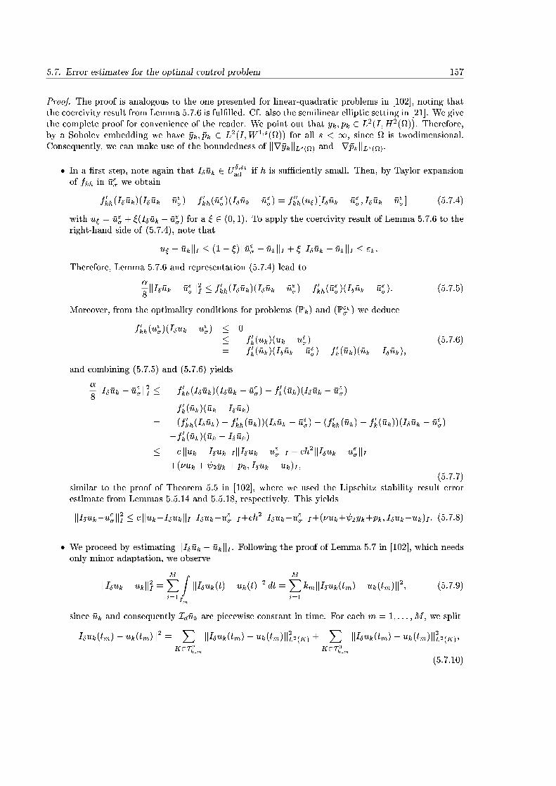
5.7. Error estimates for the optimal control problem 157
Proof. The proof is analogous to the one presented for linear-quadratic problems in [102], noting thatthe coercivity result from Lemma 5.7.6 is ful�lled. Cf. also the semilinear elliptic setting in [21]. We givethe complete proof for convenience of the reader. We point out that �yk; �pk 2 L2(I;H2()). Therefore,by a Sobolev embedding we have �yk; �pk 2 L2(I;W 1;s()) for all s < 1, since is twodimensional.Consequently, we can make use of the boundedness of kr�ykkLs() and kr�pkkLs().
� In a �rst step, note again that I��uk 2 U�;"kad if h is su�ciently small. Then, by Taylor expansionof fkh in �u"� we obtain
f 0kh(I��uk)(I��uk � �u"�)� f 0kh(�u"�)(I��uk � �u"�) = f 00kh(u�)[I��uk � �u"�; I��uk � �u"�] (5.7.4)
with u� = �u"� + �(I��uk � �u"�) for a � 2 (0; 1). To apply the coercivity result of Lemma 5.7.6 to theright-hand side of (5.7.4), note that
ku� � �ukkI � (1� �)k�u"� � �ukkI + �kI��uk � �ukkI � "k:
Therefore, Lemma 5.7.6 and representation (5.7.4) lead to
�
8kI��uk � �u"�k2I � f 0kh(I��uk)(I��uk � �u"�)� f 0kh(�u
"�)(I��uk � �u"�): (5.7.5)
Moreover, from the optimality conditions for problems (Pk) and (P"k� ) we deduce
�f 0kh(�u"�)(I��uk � �u"�) � 0� �f 0k(�uk)(�uk � �u"�)= �f 0k(�uk)(I��uk � �u"�)� f 0k(�uk)(�uk � I��uk);
(5.7.6)
and combining (5.7.5) and (5.7.6) yields
�
8kI��uk � �u"�k2I � f 0kh(I��uk)(I��uk � �u"�)� f 0k(�uk)(I��uk � �u"�)
�f 0k(�uk)(�uk � I��uk)
= (f 0kh(I��uk)� f 0kh(�uk))(I��uk � �u"�) + (f 0kh(�uk)� f 0k(�uk))(I��uk � �u"�)
�f 0k(�uk)(�uk � I��uk)
� c k�uk � I��ukkIkI��uk � �u"�kI + ch2kI��uk � �u"�kI+(��uk + 2�yk + �pk; I��uk � �uk)I ;
(5.7.7)similar to the proof of Theorem 5.5 in [102], where we used the Lipschitz stability result errorestimate from Lemmas 5.5.14 and 5.5.18, respectively. This yields
kI��uk��u"�k2I � c k�uk�I��ukkIkI��uk��u"�kI+ch2kI��uk��u"�kI+(��uk+ 2�yk+�pk; I��uk��uk)I : (5.7.8)
� We proceed by estimating kI��uk � �ukkI . Following the proof of Lemma 5.7 in [102], which needsonly minor adaptation, we observe
kI��uk � �ukk2I =MXi=1
ZIm
kI��uk(t)� �uk(t)k2 dt =MXi=1
kmkI��uk(tm)� �uk(tm)k2; (5.7.9)
since �uk and consequently Id�uk are piecewise constant in time. For each m = 1; : : : ;M , we split
kI��uk(tm)� �uk(tm)k2 =X
K2T 2h;m
kI��uk(tm)� �uk(tm)k2L2(K) +X
K2T 3h;m
kI��uk(tm)� �uk(tm)k2L2(K);
(5.7.10)
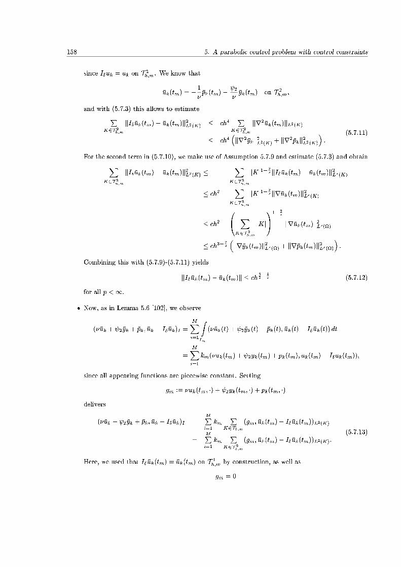
158 5. A parabolic control problem with control constraints
since I��uk = �uk on T 1h;m. We know that
�uk(tm) = �1
��pk(tm)� 2
��yk(tm) on T 2
h;m;
and with (5.7.3) this allows to estimatePK2T 2
h;m
kI��uk(tm)� �uk(tm)k2L2(K) � ch4P
K2T 2h;m
kr2�uk(tm)kL2(K)
� ch4�kr2�ykk2L2(K) + kr2�pkk2L2(K)
�:
(5.7.11)
For the second term in (5.7.10), we make use of Assumption 5.7.9 and estimate (5.7.3) and obtainXK2T 3
h;m
kI��uk(tm)� �uk(tm)k2L2(K) �X
K2T 3h;m
jKj1� 2s kI��uk(tm)� �uk(tm)k2Ls(K)
� ch2X
K2T 3h;m
jKj1� 2s kr�uk(tm)k2Ls(K)
� ch2
0@ XK2T 3
h;m
jKj1A1� 2
s
kr�uk(tm)k2Ls()
� ch3�2s
�kr�yk(tm)k2Ls() + kr�pk(tm)k2Ls()
�:
Combining this with (5.7.9)-(5.7.11) yields
kI��uk(tm)� �uk(tm)k � ch32�
1s (5.7.12)
for all p <1.
� Now, as in Lemma 5.6 [102], we observe
(��uk + 2�yk + �pk; �uk � I��uk)I =
MXi=1
ZIm
(��uk(t) + 2�yk(t) + �pk(t); �uk(t)� I��uk(t)) dt
=
MXi=1
km(��uk(tm) + 2�yk(tm) + �pk(tm); �uk(tm)� I��uk(tm));
since all appearing functions are piecewise constant. Setting
gm := ��uk(tm; �) + 2�yk(tm; �) + �pk(tm; �)delivers
(��uk + 2�yk + �pk; �uk � I��uk)I =MPi=1
kmP
K2Th;m
(gm; �uk(tm)� I��uk(tm))L2(K)
=MPi=1
kmP
K2T 3h;m
(gm; �uk(tm)� I��uk(tm))L2(K):(5.7.13)
Here, we used that I��uk(tm) = �uk(tm) on T 1h;m by construction, as well as
gm = 0

5.7. Error estimates for the optimal control problem 159
on T 2h;m. Now, by de�nition of T 3
h;m, in every cell K 2 T 3h;m there is a point xK with
gm(xK) = 0:
With (5.7.3) this implies
j(gm; I��uk(tm)� �uk(tm))L2(K)j � jKj1� 2s kgmkLs(K)kI��uk(tm)� �uk(tm)kLs(K)
= jKj1� 2s kgm � gm(xK)kLs(K)kI��uk(tm)� �uk(tm)kLs(K)
� ch2jKj1� 2s krgmkLs(K)kr�uk(tm)kLs(K)
for any 2 < s < 1. Note that an estimate like (5.7.3) can be applied to kgm � gm(xK)k, wheregm(xk) is constant.
Inserting this into (5.7.13) yields
(��uk + 2�yk + �pk; �uk � I��uk)I
�MXi=1
ckmh2X
K2T 3h;m
jKj1� 2s krgmkLs(K)kr�uk(tm)kLs(K)
�MXi=1
ckmh2(
XK2T 3
h;m
jKj)1� 2s krgmkLs()kr�uk(tm)kLs()
�MXi=1
ckmh3� 2
s krgmkLs()kr�uk(tm)kLs()
�MXi=1
ckmh3� 2
s (kr�yk(tm)kL2(I;Ls()) + kr�pk(tm)kL2(I;Ls()) + 1)kr�uk(tm)kLs()
� ch3�2s (kr�ykkL2(I;Ls()) + kr�pkkL2(I;Ls()) + 1)kr�uk(tm)kL2(I;Ls())
(5.7.14)which implies
(��uk + 2�yk + �pk; �uk � I��uk)I � ch32�
1s : (5.7.15)
� Finally, inserting (5.7.12) and (5.7.15) into (5.7.8) and applying Young's inequality yields theassertion, noting that
k�uk � �u"�kI � kI��uk � �ukkI + kI��uk � �u"�kI :
Again, we obtain that �u"� converges to �uk in L2(Q) as h tends to zero. Therefore, �u"� =: �u� is a localsolution of Problem (P�) for all h su�ciently small, and we directly obtain
Theorem 5.7.11. Let �u be an optimal solution of Problem (P), let �uk 2 B"(�u) be an optimal control ofProblem (Pk) and let Assumptions 5.7.1-5.7.9 be satis�ed. Then there exists a sequence of locally optimalcontrols to problem (Pkh) converging strongly in L2(Q) to �uk as h tends to zero, and the discretizationerror estimate
k�uk � �u�kI � C(k + h32��)
is ful�lled for every � > 0 and a constant C > 0 independent of k and h.
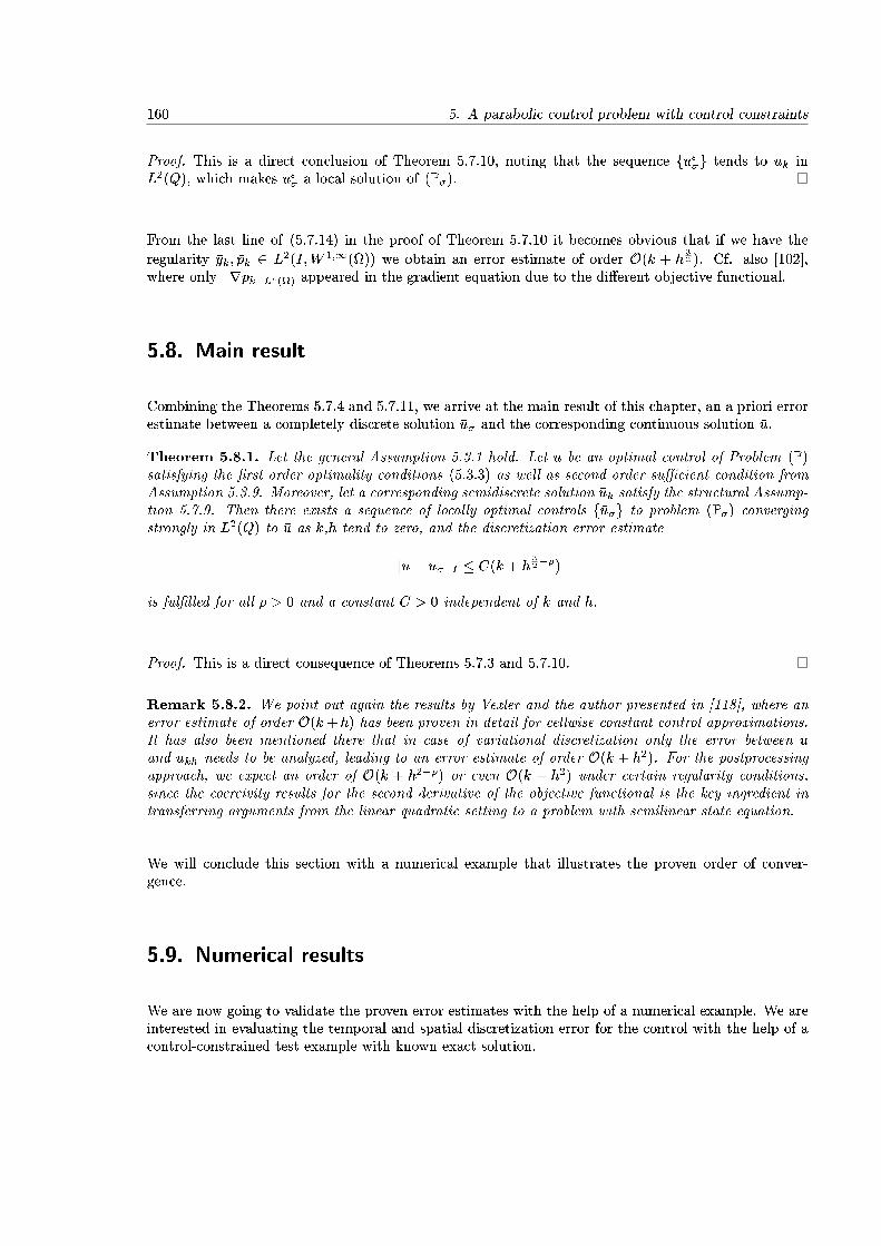
160 5. A parabolic control problem with control constraints
Proof. This is a direct conclusion of Theorem 5.7.10, noting that the sequence f�u"�g tends to �uk inL2(Q), which makes �u"� a local solution of (P�).
From the last line of (5.7.14) in the proof of Theorem 5.7.10 it becomes obvious that if we have the
regularity �yk; �pk 2 L2(I;W 1;1()) we obtain an error estimate of order O(k + h32 ). Cf. also [102],
where only kr�pkkLs() appeared in the gradient equation due to the di�erent objective functional.
5.8. Main result
Combining the Theorems 5.7.4 and 5.7.11, we arrive at the main result of this chapter, an a priori errorestimate between a completely discrete solution �u� and the corresponding continuous solution �u.
Theorem 5.8.1. Let the general Assumption 5.3.1 hold. Let �u be an optimal control of Problem (P)satisfying the �rst order optimality conditions (5.3.3) as well as second order su�cient condition fromAssumption 5.3.9. Moreover, let a corresponding semidiscrete solution �uk satisfy the structural Assump-tion 5.7.9. Then there exists a sequence of locally optimal controls f�u�g to problem (P�) convergingstrongly in L2(Q) to �u as k,h tend to zero, and the discretization error estimate
k�u� �u�kI � C(k + h32��)
is ful�lled for all � > 0 and a constant C > 0 independent of k and h.
Proof. This is a direct consequence of Theorems 5.7.3 and 5.7.10.
Remark 5.8.2. We point out again the results by Vexler and the author presented in [118], where anerror estimate of order O(k+h) has been proven in detail for cellwise constant control approximations.It has also been mentioned there that in case of variational discretization only the error between �uand �ukh needs to be analyzed, leading to an error estimate of order O(k + h2). For the postprocessingapproach, we expect an order of O(k + h2��) or even O(k + h2) under certain regularity conditions,since the coercivity results for the second derivative of the objective functional is the key ingredient intransferring arguments from the linear quadratic setting to a problem with semilinear state equation.
We will conclude this section with a numerical example that illustrates the proven order of conver-gence.
5.9. Numerical results
We are now going to validate the proven error estimates with the help of a numerical example. We areinterested in evaluating the temporal and spatial discretization error for the control with the help of acontrol-constrained test example with known exact solution.
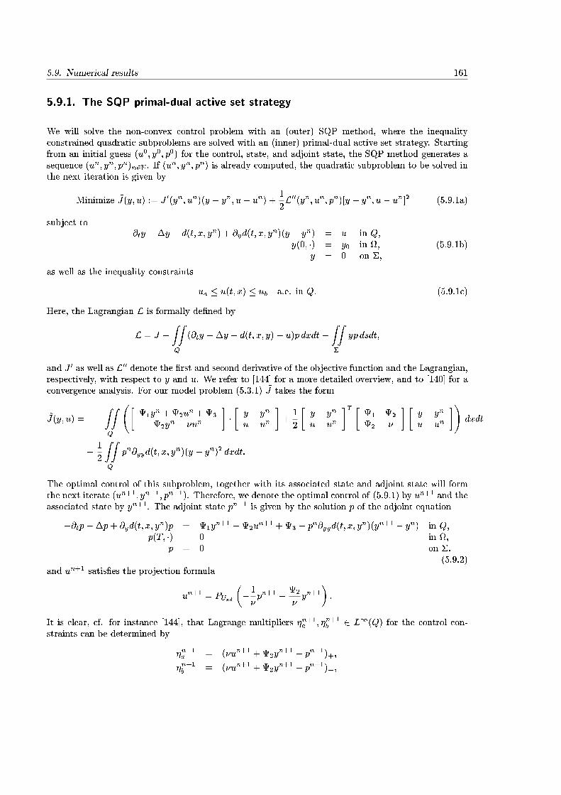
5.9. Numerical results 161
5.9.1. The SQP primal-dual active set strategy
We will solve the non-convex control problem with an (outer) SQP method, where the inequalityconstrained quadratic subproblems are solved with an (inner) primal-dual active set strategy. Startingfrom an initial guess (u0; y0; p0) for the control, state, and adjoint state, the SQP method generates asequence (un; yn; pn)n2N. If (u
n; yn; pn) is already computed, the quadratic subproblem to be solved inthe next iteration is given by
Minimize ~J(y; u) := J 0(yn; un)(y � yn; u� un) +1
2L00(yn; un; pn)[y � yn; u� un]2 (5.9.1a)
subject to@ty ��y + d(t; x; yn) + @yd(t; x; y
n)(y � yn) = u in Q;y(0; �) = y0 in ;
y = 0 on �;(5.9.1b)
as well as the inequality constraints
ua � u(t; x) � ub a.e. in Q: (5.9.1c)
Here, the Lagrangian L is formally de�ned by
L = J �ZZQ
(@ty ��y � d(t; x; y)� u)p dxdt�ZZ�
yp dsdt;
and J 0 as well as L00 denote the �rst and second derivative of the objective function and the Lagrangian,respectively, with respect to y and u. We refer to [144] for a more detailed overview, and to [140] for aconvergence analysis. For our model problem (5.3.1) ~J takes the form
~J(y; u) =
ZZQ
�1y
n +2un +3
2yn + �un
���y � yn
u� un
�+1
2
�y � yn
u� un
�T �1 2
2 �
� �y � yn
u� un
�!dxdt
� 1
2
ZZQ
pn@yyd(t; x; yn)(y � yn)2 dxdt:
The optimal control of this subproblem, together with its associated state and adjoint state will formthe next iterate (un+1; yn+1; pn+1). Therefore, we denote the optimal control of (5.9.1) by un+1 and theassociated state by yn+1. The adjoint state pn+1 is given by the solution p of the adjoint equation
�@tp��p+ @yd(t; x; yn)p = 1y
n+1 +2un+1 +3 � pn@yyd(t; x; y
n)(yn+1 � yn) in Q;p(T; �) = 0 in ;
p = 0 on �:(5.9.2)
and un+1 satis�es the projection formula
un+1 = PUad
��1
�pn+1 � 2
�yn+1
�:
It is clear, cf. for instance [144], that Lagrange multipliers �n+1a ; �n+1
b 2 L1(Q) for the control con-straints can be determined by
�n+1a = (�un+1 +2y
n+1 + pn+1)+;
�n+1b = (�un+1 +2y
n+1 + pn+1)�;
162 5. A parabolic control problem with control constraints
which we combine into a function�n+1 := �n+1
a � �n+1b :
To determine (un+1; yn+1; pn+1) as well as �n+1 an interior active set loop is used. We drop thesuperscripts n and n + 1, and introduce a subscript k, or k + 1, respectively, to indicate the iteratesof the primal-dual active set strategy, (uk; yk; pk)k2N as well as (�k)k2N, starting from u0 = un; y0 =yn; p0 = pn and �0 = �n. Known convergence results, cf. [52] guarantee that (uk; yk; pk) tends to(un+1; yn+1; pn+1). In each active set loop the active sets
Aak+1 = ((t; x) 2 Q : uk(t; x) + �k(t; x) � ua)
Abk+1 = ((t; x) 2 Q : uk(t; x) + �k(t; x) � ub)
are determined and the inequality constraints
ua � u � ub
are replaced by equality constraints of the form
uk+1 = ua on Aak+1; uk+1 = ub on Abk+1:
Noting additionally that uk+1 ful�lls
uk+1 = �1
�pk+1 � 2
�yk+1 on Ik+1 := Q n (Aak+1 [ Abk+1)
we obtain the concise representation
uk+1 := �Ik+1 � (�1
�pk+1 � 2
�yk+1) + �Aa
k+1� ua + �Ab
k+1� ub;
where �Ik+1 , �Aak+1
, and �Abk+1
denote the characteristic functions of the indexed sets. We refer for
instance to [108] for a more detailed description of the primal dual active set strategy for ellipticproblems. After obtaining the solution triple (uk+1; yk+1; pk+1), we update the multiplier
�k+1 = �uk+1 +2yk+1 + pk+1;
and determine the new active sets. The interior active set loop is terminated when the active sets intwo consecutive loops do not change.
5.9.2. Construction of a control-constrained test example
We consider a model problem in one space dimension with tracking type objective function, i.e. 1 = 1,2 = 0, as well as 3 = yd, where yd is a function to be speci�ed rather than a �xed real number. Thespatial domain and the time interval I are given by = (0; 1) as well as I = (0; T ).
Minimize1
2
TZ0
Z
((y � yd)2 + u2) dxdt (E)
subject to@ty ��y + y3 = u+ f(t; x) in Q
y(0; �) = 0 in ;y = 0 on �;
5.9. Numerical results 163
as well asua � u � ub;
with the speci�c choice
yd(t; x) = �� cos(�t) sin(�x) + �2 sin(�t) sin(�x) + 3 sin3(�t) sin3(�x) + sin(�t) sin(�x);
f(t; x) = � cos(�t) sin(�x) + �2 sin(�t) sin(�x) + sin3(�t) sin3(�x)�min
�1
2; sin(�t) sin(�x)
�;
and ua = �10 and ub = 12 .
Noting that the adjoint equation takes the form
�@tp��p+ 3�y2p = �y � yd in Qp(T; �) = 0 in ;
p = 0 on �;
direct computations verify that
�u = min
�1
2; sin(�t) sin(�x)
�together with the associated state and adjoint state
�y = sin(�t) sin(�x); �p = � sin(�t) sin(�x)
satisfy the �rst order optimality conditions of Lemma 5.3.6 or the projection formula (5.3.6). For thespeci�c setting of Problem (E) we �nd that the second derivative of the reduced objective function isgiven by
f 00(�u)[v; v] =
ZZQ
�~y2 + �v2 � 6�y�p~y2
�dxdt;
with ~y = G0(�u)v, cf. (5.3.8). We observe that
�6�y�p~y2 = 6~y2 sin2(�t) sin2 (�x) � 0:
Therefore, the second order su�cient condition from Assumption 5.3.9 is satis�ed since
f 00(�u)[v; v] =
ZZQ
�~y2 + �v2 � 6�y�p~y2
�dxdt � �kvk2I
holds, and �u is indeed an optimal solution. We will verify the error estimates for the temporal and thespatial discretization separately.
5.9.3. The error due to time discretization
We �rst solve the problem on a spatial grid with h = 2�5 for temporal meshes of size k = 2�1; : : : ; 2�11.We determine the experimental order of convergence by
EOCk =ln(k�u� �u�1k)� ln(k�u� �u�2k)
ln(k1)� ln(k2);
where k1 and k2 are consecutive (temporal) mesh sizes, and �i denotes the discretization of the PDEand the control with �xed mesh size h = 2�5 and consecutive temporal discretization parameters ki.
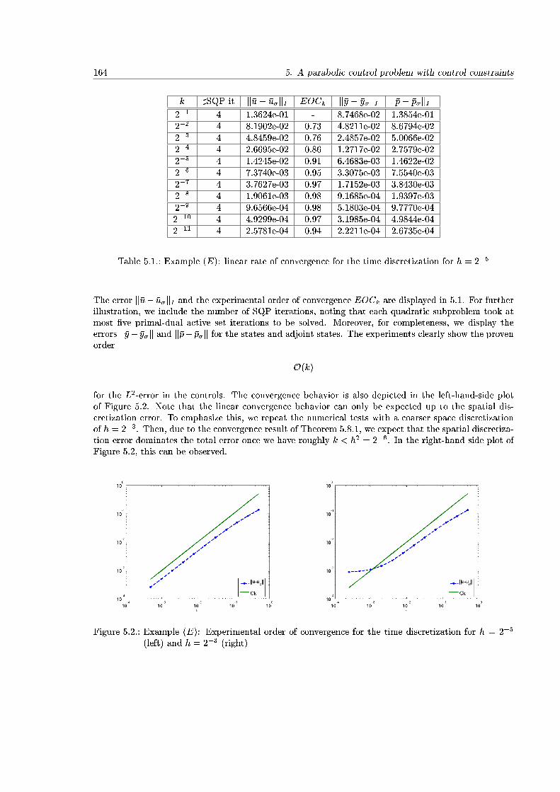
164 5. A parabolic control problem with control constraints
k ]SQP it k�u� �u�kI EOCk k�y � �y�kI �p� �p�kI2�1 4 1.3624e-01 - 8.7468e-02 1.3854e-012�2 4 8.1902e-02 0.73 4.8211e-02 8.6794e-022�3 4 4.8459e-02 0.76 2.4857e-02 5.0066e-022�4 4 2.6695e-02 0.86 1.2717e-02 2.7579e-022�5 4 1.4245e-02 0.91 6.4683e-03 1.4622e-022�6 4 7.3740e-03 0.95 3.3075e-03 7.5540e-032�7 4 3.7627e-03 0.97 1.7152e-03 3.8430e-032�8 4 1.9061e-03 0.98 9.1685e-04 1.9397e-032�9 4 9.6566e-04 0.98 5.1803e-04 9.7770e-042�10 4 4.9299e-04 0.97 3.1985e-04 4.9844e-042�11 4 2.5781e-04 0.94 2.2211e-04 2.6735e-04
Table 5.1.: Example (E): linear rate of convergence for the time discretization for h = 2�5
The error k�u� �u�kI and the experimental order of convergence EOCk are displayed in 5.1. For furtherillustration, we include the number of SQP iterations, noting that each quadratic subproblem took atmost �ve primal-dual active set iterations to be solved. Moreover, for completeness, we display theerrors k�y� �y�k and k�p� �p�k for the states and adjoint states. The experiments clearly show the provenorder
O(k)
for the L2-error in the controls. The convergence behavior is also depicted in the left-hand-side plotof Figure 5.2. Note that the linear convergence behavior can only be expected up to the spatial dis-cretization error. To emphasize this, we repeat the numerical tests with a coarser space discretizationof h = 2�3. Then, due to the convergence result of Theorem 5.8.1, we expect that the spatial discretiza-tion error dominates the total error once we have roughly k < h2 = 2�6. In the right-hand side plot ofFigure 5.2, this can be observed.
Figure 5.2.: Example (E): Experimental order of convergence for the time discretization for h = 2�5
(left) and h = 2�3 (right)
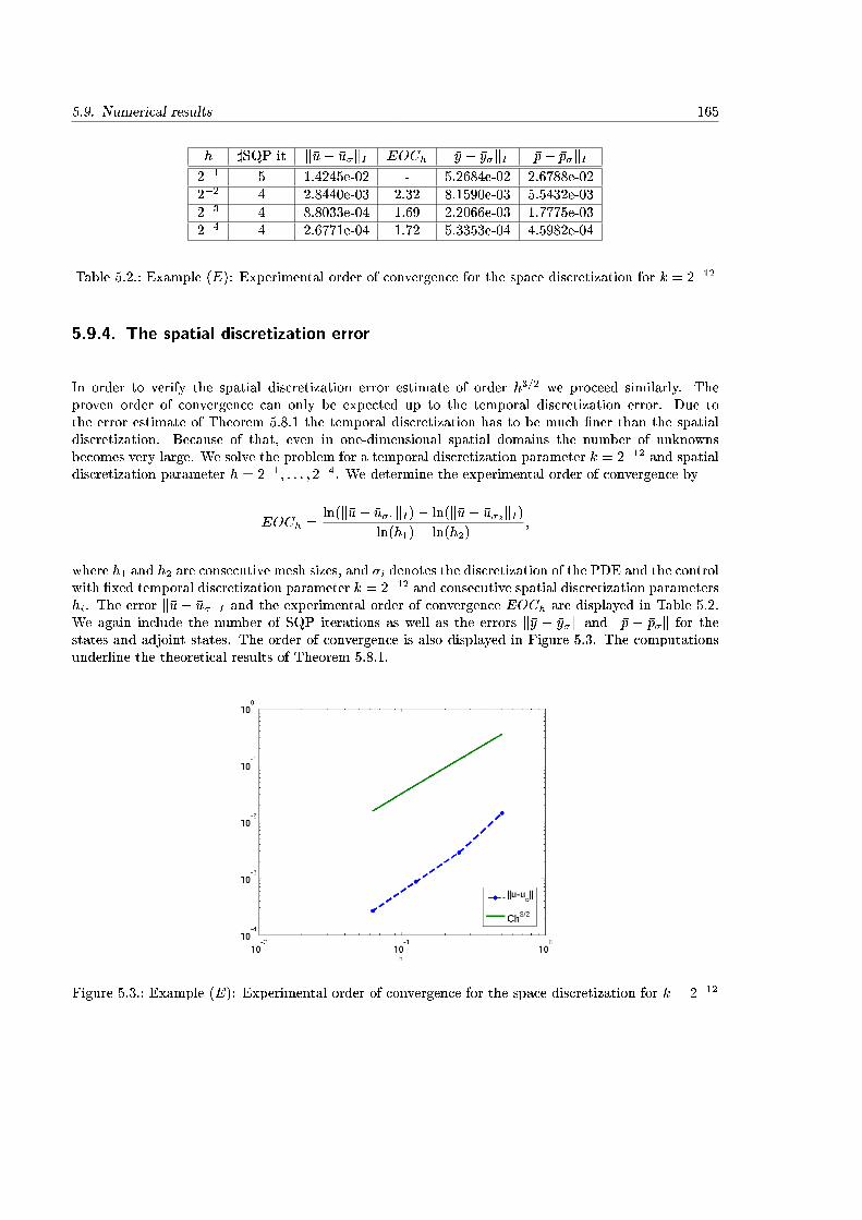
5.9. Numerical results 165
h ]SQP it k�u� �u�kI EOCh k�y � �y�kI �p� �p�kI2�1 5 1.4245e-02 - 5.2684e-02 2.6788e-022�2 4 2.8440e-03 2.32 8.1590e-03 5.5432e-032�3 4 8.8033e-04 1.69 2.2066e-03 1.7775e-032�4 4 2.6771e-04 1.72 5.3353e-04 4.5982e-04
Table 5.2.: Example (E): Experimental order of convergence for the space discretization for k = 2�12
5.9.4. The spatial discretization error
In order to verify the spatial discretization error estimate of order h3=2 we proceed similarly. Theproven order of convergence can only be expected up to the temporal discretization error. Due tothe error estimate of Theorem 5.8.1 the temporal discretization has to be much �ner than the spatialdiscretization. Because of that, even in one-dimensional spatial domains the number of unknownsbecomes very large. We solve the problem for a temporal discretization parameter k = 2�12 and spatialdiscretization parameter h = 2�1; : : : ; 2�4. We determine the experimental order of convergence by
EOCh =ln(k�u� �u�1kI)� ln(k�u� �u�2kI)
ln(h1)� ln(h2);
where h1 and h2 are consecutive mesh sizes, and �i denotes the discretization of the PDE and the controlwith �xed temporal discretization parameter k = 2�12 and consecutive spatial discretization parametershi. The error k�u � �u�kI and the experimental order of convergence EOCh are displayed in Table 5.2.We again include the number of SQP iterations as well as the errors k�y � �y�k and k�p � �p�k for thestates and adjoint states. The order of convergence is also displayed in Figure 5.3. The computationsunderline the theoretical results of Theorem 5.8.1.
Figure 5.3.: Example (E): Experimental order of convergence for the space discretization for k = 2�12

166 5. A parabolic control problem with control constraints
5.9.5. The regularization error
To conclude this section, we demonstrate how a purely state-constrained optimal control problem canbe solved via regularization. We consider a special setting of Problem (5.2.1) in Q := (0; 1) � (0; 1),given by
Minimize1
2
1Z0
Z
((y � yd)2 + u2) dxdt (E�)
subject to@ty ��y + y3 = u+ f(t; x) in Q
y(0; �) = sin(�x) in ;y = 0 on �;
as well as�1 � y � 1;
with the speci�c choice
yd(t; x) = sin(�x) + (jx� 1
2j � 1
2)� 3 sin2(�x)(t� 1)
�jx� 1
2j � 1
2
�;
f(t; x) = �2 sin(�x) + sin3(�x) + (t� 1)(jx� 1
2j � 1
2):
The adjoint equation takes the form
�@tp��p+ 3�y2p = �y � yd + ��b;Q � ��a;Q in Qp(1; �) = �y � yd + ��b;T � ��a;T in ;
p = 0 on �;
and direct computations verify that
�u = �(t� 1)
�����x� 1
2
����� 1
2
�together with the associated state and adjoint state
�y = sin(�x); �p = (t� 1)
�����x� 1
2
����� 1
2
�;
as well as the Lagrange multipliers ��a = 0 and ��b = 2(t�1)�x= 12satisfy �rst order optimality conditions
similar to Theorem 4.2.8, i.e. with Uad = L1(Q). Note in particular that �u 2 L1(Q). Moreover, theproblem is constructed with very low regularity of the adjoint state due to the presence of Dirac measuresin the right-hand side. Second order su�cient conditions are again veri�ed by noting that
�@yd(�; �y)�p = �3�y2�p > 0:
The problem is regularized by Lavrentiev regularization and transformed into a control-constrainedproblem as pointed out in Section 5.2. We then solve the regularized problem with discretizationparameters k = 2�10 and h = 2�5 for decreasing values of � = �1; : : : ; �6. We choose �i = 10�i
and take the solution pertaining to �i�1 as an initial guess for the SQP method for i > 1. For anextrapolation based strategy to initialize the solution algorithm we refer to [70] for elliptic problems.In Table 5.3, we display for each � the number of SQP iterations and the overall number of primal-dual-active set iterations, as well as the L2-error for the control, the state, and the adjoint state. Of
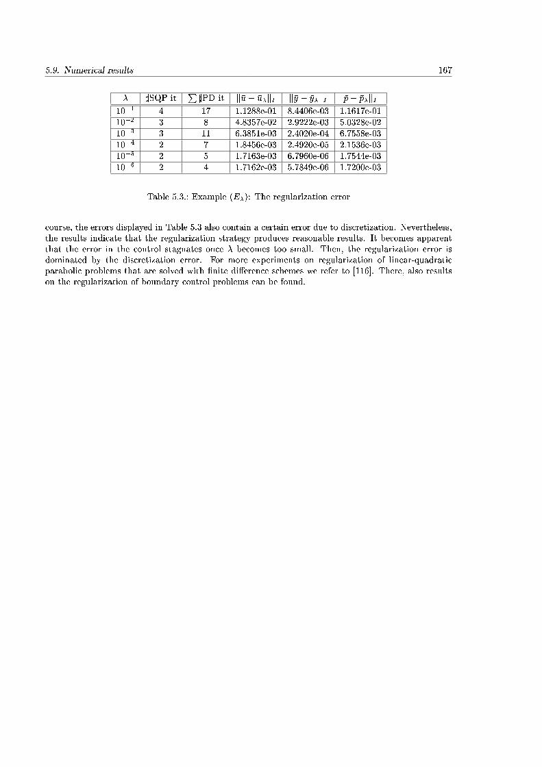
5.9. Numerical results 167
� ]SQP itP]PD it k�u� �u�kI k�y � �y�kI �p� �p�kI
10�1 4 17 1.1288e-01 8.4406e-03 1.1617e-0110�2 3 8 4.8357e-02 2.9222e-03 5.0328e-0210�3 3 11 6.3851e-03 2.4020e-04 6.7558e-0310�4 2 7 1.8456e-03 2.4920e-05 2.1536e-0310�5 2 5 1.7163e-03 6.7960e-06 1.7544e-0310�6 2 4 1.7162e-03 5.7849e-06 1.7200e-03
Table 5.3.: Example (E�): The regularization error
course, the errors displayed in Table 5.3 also contain a certain error due to discretization. Nevertheless,the results indicate that the regularization strategy produces reasonable results. It becomes apparentthat the error in the control stagnates once � becomes too small. Then, the regularization error isdominated by the discretization error. For more experiments on regularization of linear-quadraticparabolic problems that are solved with �nite di�erence schemes we refer to [116]. There, also resultson the regularization of boundary control problems can be found.

6. Conclusion and outlook
In this thesis, we have made some new contributions to the theoretical and numerical analysis ofnonconvex PDE constrained optimal control problems. The focus has been placed on model problemswith pointwise state constraints.
As a �rst model problem, we have discussed a semi-in�nite optimal control problem arising from anelliptic PDE constrained model problem with �nite dimensional control space and state constraints ona set of positive measure. While the theory for the model problem with respect to �rst and secondorder optimality conditions is known, the novelty of this chapter lies in the a priori �nite elementerror estimates for the control. The available theory of error estimates for elliptic control-constrainedproblems is rather rich, but less is known for state-constrained optimal control problems, cf. also thereferences given in Chapters 1 and 3. Relying on some assumptions that are typically made in optimalcontrol, we additionally assumed a certain structure of the active sets that is natural in semi-in�niteprogramming. That is, we assumed that the bound on the state is only active in �nitely many points.In contrast to the situation considered in [106], the location of these active points is assumed unknownand the bounds are therefore prescribed in a subset of . The di�erence to the model problem from[106] also becomes obvious in the �nal results. Only under certain conditions does the error of thestate equation re ect upon the convergence of the discrete optimal controls. This is due to the factthat the controls can vary more freely since the active points of the states may change as well. Weprovided conditions that ensure an error estimate of order h2j lnhj and also demonstrated that in othersituations the lower order estimate of order h
pj lnhj is sharp. Throughout, we took into account thatthe nonconvex problem may admit multiple local solutions. These results have been published for linear-quadratic problems in [104, 105]. The extension to semilinear state equations required some additionalconsiderations such as second order su�cient conditions and �nding an adequate substitute for thesuperposition principle. We have shown some numerical examples to underline the theoretical results.Our main focus has been on the development of the error estimates rather than on the implications innumerical computations. It will be interesting to investigate if and how the results can be of advantagein numerical solution algorithms. Another interesting question is to consider di�erent types of bounds.A fundamental ingredient in our convergence proofs was the fact that due to the constant bounds andthe linear �nite element approximation the state constraints could be prescribed in the grid points onlywithout changing the admissible sets in the neighborhood of local solutions. For more general boundson the state, and additional contribution to the �nal error estimate is to be expected, cf. also [4].
In addition to the state-constrained elliptic problem we were interested in the analysis of time-dependent,parabolic formulations, where we admit control functions that can vary arbitrarily in space and time.The challenges of pointwise state constraints for the considered problem class are well-known. InChapter 4, we therefore focused on the analysis of a well-established regularization method. We ap-plied Lavrentiev regularization that transforms pointwise state constraints into mixed control-stateconstraints, and obtained a problem formulation that behaves well with respect to �rst and secondorder optimality conditions. There are two main new contributions in this chapter: On the one hand,we provided the stability analysis of an associated linearized problem that eventually led to the strongregularity for generalized equations that represent the �rst order optimality conditions for the regu-larized nonlinear problem. This property is a fundamental condition for many results related to the
169
170 6. Conclusion and outlook
analysis of numerical solution algorithms. We used it primarily to deduce a local uniqueness prop-erty of a well-de�ned locally optimal control, but it could also be used to deduce convergence of SQPmethods. Similar results for elliptic control problems have been provided in [7] and [61, 60]. We pointout, however, that the lower regularity properties of parabolic equations require special attention. Asecond important result of this chapter is the regularization error estimate, and the convergence resultfor regularization parameter � tending to zero, that were only available for elliptic problems, cf. [31].Most of the results have been published in [115], cf. also [114].
Finally, Chapter 5 was devoted to the �nite element error estimates for certain parabolic optimal controlproblems. We began this chapter by showing how a problem with Lavrentiev-regularized mixed control-state constraints and no further control constraints can be transformed into a purely-control-constrainedmodel problem, cf. also [111]. This transformation had already been used by Hinze and Meyer, cf. [73]to obtain �nite element error estimates for a variational discretization of elliptic Lavrentiev regularizedproblems. However, the lower regularity properties of the parabolic control-to-state operator made theconvergence analysis for Lavrentiev parameters tending to zero a delicate issue, even more so thanin Chapter 4. We have proven convergence under certain assumptions adapting arguments from theelliptic setting, cf. [69]. For linear-quadratic problems, this has been published in [116]. We thenderived a priori error estimates for the �nite element discretization of a parabolic control-constrainedmodel problem in two-dimensional spatial domains with semilinear state equation that also includesLavrentiev regularized problems discussed at the beginning of Chapter 5. The problems are discretizedby a discontinuous Galerkin scheme in time and usual conforming �nite elements in space. The controlsthemselves were discretized piecewise constant in time and cellwise bilinear in space. We extended theresults from [102] for linear quadratic problems to problems with semilinear state equation. This is anew contribution to the �nite element error analysis of parabolic optimal control problems where thetheory is less complete than in the elliptic setting, cf. also the introductory remarks in Chapter 1. Forthe considered problem class we were able to provide and use a quadratic growth condition for locallyoptimal controls in an L2-neighborhood, thus avoiding the need for convergence in L1(I�). However,we needed a uniform boundedness result for solutions of the semidiscrete and discrete state equation.The former was obtained by applying Stampacchia's method to the semidiscrete system of equations,whereas the latter followed essentially from appropriate error estimates between the semidiscrete andthe discrete level. We eventually obtained an error estimate of order O(k + h
32�"), " > 0, where
k denotes the temporal discretization parameter and h denotes the spatial discretization parameter.These results have been published in [118] for a slightly di�erent objective function, with a detailedproof of convergence for controls that are discretized by piecewise constants in time and space. Thischange in the objective function was mainly motivated by our interest in state constrained controlproblems. At the end of Chapter 5 we have also provided some numerical examples that underline thetheoretical results.
A. Supplementary results
A.1. Function spaces
We give a brief overview about the function spaces used in this thesis. For further information we pointout textbooks on functional analysis, e.g. [1] and partial di�erential equations, e.g. [48]. An overviewrelevant for optimal control with PDEs can also be found in [144], whose notation we adopt here andwhere the following de�nitions can be found.
A.1.1. Lp-spaces, Sobolev spaces, and spaces of continuous functions
De�nition A.1.1. By fLp(); k � kLp()g; 1 � p � 1; we denote the Banach space of all Lebesguemeasurable functions v de�ned on that satisfy
R
jv(x)jpdx < 1, or in case of p = 1 are essentiallybounded, respectively, whose norms are given by
kvkLp() :=0@Z
jv(x)jpdx1A
1p
; kvkL1() := ess supx2
jv(x)j := infjF=0j
sup
x2nFjv(x)j
!:
The case p = 2 is of special interest, and we note that L2() is even a Hilbert space with the innerproduct
(v; w)L2() :=
Z
vwdx:
De�nition A.1.2. By Ck(), we denote the linear space of all real-valued functions on that, togetherwith their partial derivatives up to order k, are continuous on . Moreover, Ck(�) denotes the spaceof all elements of Ck() that, together with their partial derivatives up to order k, can be continuouslyextended to �. We agree on the short notation C(�) instead of C0(�). The space Ck(�) is a Banachspace with norm
kvkC(�) := maxx2�
jv(x)j; kvkCk(�) :=Xj�j�k
kD�vkC(�);
where � is a multi-index. Last, for a positive real number �, we introduce the space Ck;�(�) of allfunctions g 2 Ck(�) that, together with their partial derivatives up to order k, are H�older continuous,i.e.
jD�g(x1)�D�g(x2)j � Cjx1 � x2j�Rn ; 8 j�j � k
for a constant C > 0.
171
172 A. Supplementary results
Since we will look for solutions of the governing PDEs in weak sense, we introduce the Sobolev spacesW k;p(). We brie y recall that a weak derivative of order j�j; w 2 L1
loc() of u 2 L1loc() is de�ned
by Z
u(x)D�v(x)dx = (�1)j�jZ
w(x)v(x)dx 8 v 2 C10 ();
where � is a multiindex, L1loc() denotes the space of locally Lebesgue integrable functions, and the
subscript 0 in C10 () indicates functions with compact support in .
De�nition A.1.3. Let 1 � p � 1 and k 2 N be given. We denote by W k;p() the linear space of allfunctions v 2 Lp() having weak derivatives D�v in Lp() for all multi-indices � of length j�j � k,endowed with the norm
kvkWk;p() =
0@Xj�j�k
Z
jD�v(x)jpdx1A
1p
; kvkWk;1() = maxj�j�k
kD�vkL1();
for p < 1 and p = 1, respectively. We write in short Hk() := W k;2(). H1() becomes a Hilbertspace with the associated inner product
(u; v)H1() :=
Z
uvdx+
Z
rurvdx:
To incorporate the Dirichlet boundary conditions in a meaningful way, we introduce
H10 () :=W 1;2
0 () = fv 2 H1(): vj� = 0g; kvkH10 ()
=
0@Z
jrj2dx1A
12
;
where W k;p0 () denotes the closure of C10 ().
A.1.2. Spaces of vector valued functions
Spaces like Lp() and C() can be extended to other domains, e.g. time-space domains Q, simply byreplacing by Q. A fundamental tool for treating nonstationary equations is the concept of abstractfunctions, i.e. mappings from an interval [a; b] � R, e.g. a time interval I := (0; T ), into a Banach spaceX. We will mainly make use of the following spaces, cf. [144].
Let fX; k � kXg be a real Banach space.
De�nition A.1.4. We denote the space of all abstract functions that are continuous at every t 2 [a; b]by C([a; b]; X). This space is a Banach space with norm kvkC([a;b];X) = max
t2[a;b]kvkX .
De�nition A.1.5. We denote by Lp(a; b;X), 1 � p < 1, the linear space of all measurable abstractfunctions v : [a; b]! X with the property
bZa
kv(t)kpXdt <1:
A.1. Function spaces 173
This space becomes a Banach space when endowed with respect to the norm
kvkLp(a;b;X) :=
0@ bZa
kv(t)kpXdt1A
1p
:
The space L1(a; b;X) denotes the space of all measurable abstract functions v : [a; b] ! X having theproperty that
kvkL1(a;b;X) := ess sup[a;b]
kv(t)kX <1:
If X = Lp() with p < 1, the space Lp([a; b]; Lp() can be identi�ed with Lp([a; b] � ). For p = 1,we only obtain L1([a; b]; L1()) � L1([a; b]� ).
De�nition A.1.6. We denote by H1([a; b];X) the space of all abstract functions v : [a; b] ! X withv 2 L2(X) and @tv 2 L2(X), with norm
kvk2H1([a;b];X) := kvk2L2(a;b;X) + k@tvk2L2(a;b;L2(X):
Last, let us introduce a state space with less regularity of the time derivatives.
De�nition A.1.7. Let V be a Banach space with dual space V �. We denote by W(0; T ) the linearspace of
W(0; T ) = fv 2 L2(0; T; V ) j @tv 2 L2(0; T; V �gwith the norm
kvkW(0;T ) =
0@ TZ0
(kv(t)k2V + kv0(t)k2V �)dt1A
12
We mention here that the dual space of a Banach space fX; k � kXg, denoted by X�, is the space ofall continuous linear functionals on fX; k � kXg. For Hilbert spaces (H; (�; �)), the Riesz representationtheorem guarantees that for each continuous linear functional F 2 H� there exists a uniquely determinedf 2 H such that
kFkH� = kfkH ; F (v) = (f; v)H 8v 2 H:For Lp-spaces with 1 < p <1, we have
Lp()� �= Lq();1
p+1
q= 1:
Also, we have
L1()� �= L1();
but unfortunately L1()� cannot be identi�ed with L1(). Instead, the elements of L1()� admitvery low regularity, which makes L1() an unsuitable state space in the context of state-constrainedoptimal control problems. We refer to [134] for a discussion of Lagrange multipliers in these spaces.On the other hand, the dual space of C(�) can at least be identi�ed with the space of regular Borelmeasures, M(�), cf. [6].
174 A. Supplementary results
A.2. Some properties of the control-to-state operators
We will provide the proof of Lemma 3.1.4, which states the Lipschitz-continuity of the control-to-state-operator and the objective function and their derivatives for the elliptic semi-in�nite problem, and itsparabolic counterpart, Lemma 4.2.4. The techniques are similar, yet in the elliptic case we only dealwith �nitely many control parameters, whereas the functions from the parabolic setting require somecaution with respect to the appearing norms.
A.2.1. Proof of Lemma 3.1.4
Proof. For u1; u2 and v given consider yi = G(ui), ~yi = G0(ui)v and yi = G00(ui)[v; v]. For the �rstestimate, it will be convenient to use the weak formulations of the appearing PDEs. We �rst prove(3.1.6). The di�erence z := y1 � y2 ful�lls
a(z; ') = (d(�; y2; u2)� d(�; y1; u2); ') + (d(�; y1; u2)� d(�; y1; u1); ') 8' 2 V: (A.2.1)
Testing (A.2.1) with ' = z yields
c kzk2H10 ()
� (d(�; y2; u2)� d(�; y1; u2); z) + (d(�; y1; u2)� d(�; y1; u1); z) (A.2.2)
by the H10 ()-ellipticity of a. The monotonicity of d with respect to y implies
(d(�; y2; u2)� d(�; y1; u2); z) � 0;
and the local Lipschitz continuity with respect to u gives rise to
(d(�; y1; u2)� d(�; y1; u1); z) � ckd(�; y1; u2)� d(�; y1; u1)kkzk � cju1 � u2jkzk;
where c can be taken independently of u1; u2 by the boundedness of Uad. Insertion of both estimatesin (A.2.2) yields
kzk2H10 ()
� cju1 � u2jkzk � cju1 � u2jkzkH10 ()
;
due to Friedrich's inequality applied to the left hand side. After dividing by kzkH10 ()
we obtain
Lipschitz stability in H1() and thus also in L2(). The estimate in the norm C(�) follows by applyingProposition 2.4.2 to the linear equation
Az = d(�; y2; u2)� d(�; y1; u1) in ;z = 0 on �;
which due to the Lipschitz properties of d and the fact that ky1 � y2k can be estimated as just provenyields
kzkC(�) � c (ky1 � y2k+ ju1 � u2j) � cju1 � u2j:Now, to prove (3.1.7), consider the di�erence ~z = ~y1 � ~y2, which ful�lls
A~z + @yd(�; y1; u1)~z = (@yd(�; y2; u2)� @yd(�; y1; u1))~y2 + (@ud(�; y2; u2)� @ud(�; y1; u1))v in ~z = 0 on �
By the Lipschitz continuity of @ud and @yd, we obtain
k~zkL2()\H1()\C(�) � c(ky1 � y2k1 + ju1 � u2j)(k~y2k+ jvj) � cju1 � u2jjvj;
A.2. Some properties of the control-to-state operators 175
where we applied Proposition 2.4.2, and the Lipschitz estimate (3.1.6), as well as the boundedness ofUad. Estimate (3.1.8), i.e. the Lipschitz stability for the second derivative G00 is proven in a similarway, taking into account the Lipschitz continuity of d00. To demonstrate this consider z := y1 � y2,which ful�lls
Az + @yd(�; y1; u1)z = (@yd(�; y2; u2)� @yd(�; y1; u1))y2 + (~y; 0T )d00(�; y2; u2)(~y2; vT )T+(~y1; v
T )(d00(�; y2; u2)� d00(�; y1; u1))(~y2; vT )T+(~y1; v
T )d00(�; y1; u1))(~y; 0T )T in
z = 0 on �:
Then, Proposition 2.4.2 combined with the Lipschitz properties of d and its derivatives, as well as theboundedness of Uad yields
kzkL2()\H1()\C() �c(ky1 � y2k1 + ju1 � u2j)ky2k+ c(k~yk1(k~y2k1 + jvj)+ c(k~y1k1 + jvj)(ky1 � y2k1 + ju1 � u2j)(k~y2k1 + jvj) + ck~yk1(k~y1k1 + jvj):
Note that some parts of the right-hand-side could have been estimated in weaker norms. Nevertheless,noting that
ky1 � y2k1 � cju1 � u2jby (3.1.6), as well as
k~yk1 + k~y1k1 + k~y2k1 � cjvjby Proposition 2.4.2, which then implies
kz2k � cjvj2;we �nally obtain
kykL2()\H1()\C() � cju1 � u2jjvj2:For the objective function, we proceed in a similar way. Estimate (3.1.9) is a simple conclusion of theLipschitz properties of and (3.1.6), since
jf(u1)� f(u2)j �Z
j(x; y1(x); u1)�(x; y2(x); u2)j dx � c(ky1 � y2k+ ju1 � u2j) � c ju1 � u2j
is satis�ed. To prove (3.1.10), not that the �rst derivative satis�es
jf 0(u1)v � f 0(u2)vj �Z
j@u(x; y1; u1)v � @u(x; y2; u2)v + @y(x; y1; u1)~y1 � @y(x; y2; u2)~y2j dx
�Z
j (@u(x; y1; u1)� @u(x; y2; u2)) v + @y(x; y1; u1)(~y1 � ~y2)
+ (@y(x; y1; u1)� @y(x; y2; u2)) ~y2j dx�c (ky1 � y2k1 + ju1 � u2j) jvj+ cju1 � u2jjvj+ c (ky1 � y2k1 + ju1 � u2j) jvj�c ju1 � u2jjvj
by (3.1.9) as well as Proposition 2.4.2. Estimate (3.1.11) for the second derivative, we obtain by straight-forward calculations:
jf 00(u1)[v; v]� f 00(u2)[v; v]j �Z
j(~y; 0T )00(�; y2; u2)(~y2; vT )T
+ (~y1; vT )(00(�; y2; u2)�00(�; y1; u1))(~y2; vT )T
+ ((~y1; vT )00(�; y1; u1))(~y; 0T )T j dx;
The right-hand-side can be estimated completely analogously to the previous estimates.
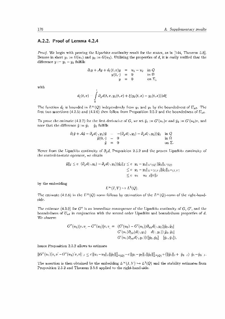
176 A. Supplementary results
A.2.2. Proof of Lemma 4.2.4
Proof. We begin with proving the Lipschitz continuity result for the states, as in [144, Theorem 5.8].Denote in short y1 := G(u1) and y2 := G(u2). Utilizing the properties of d, it is easily veri�ed that thedi�erence y := y1 � y2 ful�lls
@ty +Ay + d�(t; x)y = u1 � u2 in Qy(0; �) = 0 in
y = 0 on �;
with
d�(t; x) =
1Z0
@yd(t; x; y1(t; x) + �(y2(t; x)� y1(t; x)))d�
The function d� is bounded in L1(Q) independently from y1 and y2 by the boundedness of Uad. The�rst two assertions (4.2.5) and (4.2.6) then follow from Proposition 2.5.2 and the boundedness of Uad.
To prove the estimate (4.2.7) for the �rst derivative of G, we set ~y1 := G0(u1)v and ~y2 := G0(u2)v, andnote that the di�erence ~y := ~y1 � ~y2 ful�lls
@t~y +A~y + @yd(�; y1)~y = �(@yd(�; y1)� @yd(�; y2))~y2 in Q~y(0; �) = 0 in
~y = 0 on �:
Hence from the Lipschitz continuity of @yd, Proposition 2.5.2 and the proven Lipschitz continuity ofthe control-to-state operator, we obtain
k~ykI � c k(@yd(�; y1)� @yd(�; y2))~y2kI � c ky1 � y2kL4(Q)k~y2kL4(Q)
� c ky1 � y2kL1(I;V )k~y2kL1(I;V )
� c ku1 � u2kIkvkIby the embedding
L1(I; V ) ,! L4(Q):
The estimate (4.2.8) in the L1(Q) norm follows by estimation of the L1(Q)-norm of the right-hand-side.
The estimate (4.2.9) for G00 is an immediate consequence of the Lipschitz continuity of G, G0, and theboundedness of Uad in conjunction with the second order Lipschitz and boundedness properties of d.We observe
G00(u1)[v; v]�G00(u2)[v; v] = (G0(u2)�G0(u1))@yyd(�; y2)[~y2; ~y2]+G0(u1)@yy(d(�; y2)� d(�; y1))[~y2; ~y2]+G0(u1)@yyd(�; y1))([~y2; ~y2]� [~y1; ~y1]);
hence Proposition 2.5.2 allows to estimate
kG00(u1)[v; v]�G00(u2)[v; v]kI � c ku1�u2kIk~y2k2L4(Q)+c ky1�y2kIk~y2k2L4(Q)+(k~y1kI+k~y2kI)k~y1�~y2kI :
The assertion is then obtained by the embedding L1(I; V ) ,! L4(Q) and the stability estimates fromProposition 2.5.2 and Theorem 2.5.6 applied to the right-hand-side.

A.3. Proof of Theorem 5.5.1 177
The �rst estimate (4.2.10) for the objective function is trivial. Direct calculations show that
jf 0(u1)v � f 0(u2)vj�
ZZQ
j@y(t; x; y1; u1)~y1 � @y(t; x; y2; u2)~y2 + @u(t; x; y1; u1)v � @u(t; x; y2; u2)vj dxdt
�ZZQ
j@y(t; x; y1; u1)(~y1 � ~y2) + (@y(t; x; y1; u1)� @y(t; x; y2; u2))~y2
+ (@u(t; x; y1; u1)� @u(t; x; y2; u2))vj dxdt
Then, by the Lipschitz properties of and its derivatives, we can estimate
jf 0(u1)v � f 0(u2)vj � ck~y1 � ~y2kI + c(ky1 � y2kI + ku1 � u2kI)(k~y2kI + kvkI):
Applying Lipschitz results for G and G0, and Proposition 2.5.2 to the right-hand-side yields the desiredestimate (4.2.11) for the �rst derivative. Moreover, we have
jf 00 (u1)[v; v]� f 00(u2)(v; v)j
�ZZQ
����� �
~y0
�T �@yy(t; x; y1; u1) @yu(t; x; y1; u1)@uy(t; x; y1; u1) @uu(t; x; y1; u1)
� �~y1v
�
+
�~y2v
�T ��@yy(�; y1; u1) @yu(�; y1; u1)@uy(�; y1; u1) @uu(�; y1; u1)
���@yy(�; y2; u2) @yu(�; y2; u2)@uy(�; y2; u2) @uu(�; y2; u2)
���~y1v
�+
�~y2v
�T �@yy(�; y2; u2) @yu(�; y2; u2)@uy(�; y2; u2) @uu(�; y2; u2)
� �~y0
�!����� dxdt+
ZZQ
(@y(t; x; y1; u1)(y) + (@y(t; x; y1; u1)� @y(t; x; y2; u2)y2)) dxdt:
Then we estimate
jf 00(u1)[v; v]� f 00(u2)[v; v]j � c(k~y1 � ~y2kI(k~y1kI + kvkI)+(k~y2kI + kvkI(kyk1;1 + ku1 � u2k1;1)(k~y1kI + kvkI)(k~y2kI + kvkI)k~y1 � ~y2kI + kykI + (kykI + ku1 � u2kI)ky2kI):
The boundedness of Uad and 00, Proposition 2.5.2 as well as the Lipschitz continuity results for G, G0
and G00 yield the last estimate (4.2.12).
A.3. Proof of Theorem 5.5.1
Proof. Let k and h be �xed. We discuss only the �rst time interval I1. We obtain the formulation
k1(rykh;1;r'1) + (ykh;1; '1) + (d(t; x; ykh;1); '1)I1 = (u; '1)I1 + (y0; '1) 8'1 2 Vh;
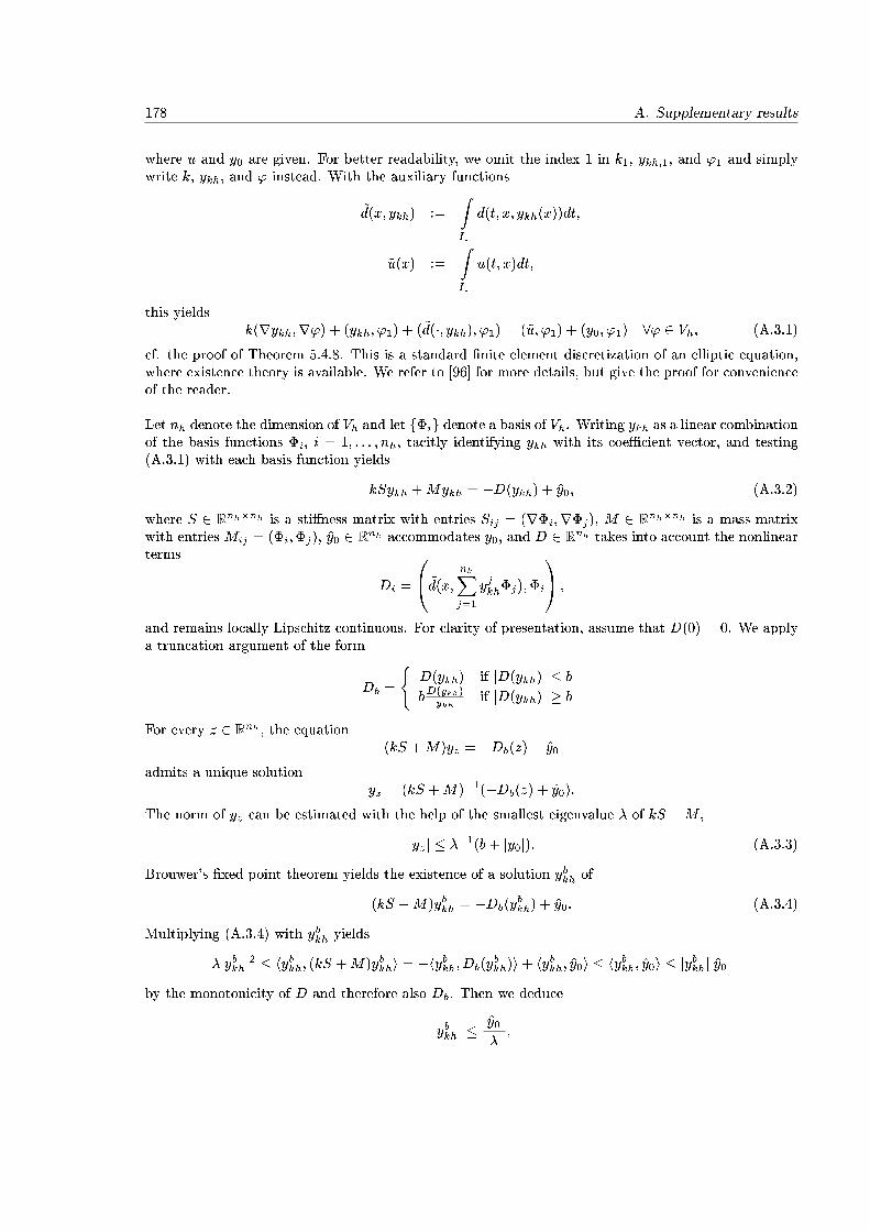
178 A. Supplementary results
where u and y0 are given. For better readability, we omit the index 1 in k1, ykh;1, and '1 and simplywrite k, ykh, and ' instead. With the auxiliary functions
~d(x; ykh) :=
ZI1
d(t; x; ykh(x))dt;
~u(x) :=
ZI1
u(t; x)dt;
this yieldsk(rykh;r') + (ykh; '1) + ( ~d(�; ykh); '1) = (~u; '1) + (y0; '1) 8' 2 Vh; (A.3.1)
cf. the proof of Theorem 5.4.8. This is a standard �nite element discretization of an elliptic equation,where existence theory is available. We refer to [96] for more details, but give the proof for convenienceof the reader.
Let nh denote the dimension of Vh and let f�ig denote a basis of Vh. Writing ykh as a linear combinationof the basis functions �i, i = 1; : : : ; nh, tacitly identifying ykh with its coe�cient vector, and testing(A.3.1) with each basis function yields
kSykh +Mykh = �D(ykh) + y0; (A.3.2)
where S 2 Rnh�nh is a sti�ness matrix with entries Sij = (r�i;r�j), M 2 Rnh�nh is a mass matrixwith entries Mij = (�i;�j), y0 2 Rnh accommodates y0, and D 2 Rnh takes into account the nonlinearterms
Di =
0@ ~d(x;
nhXj=1
yjkh�j);�i
1A ;
and remains locally Lipschitz continuous. For clarity of presentation, assume that D(0) = 0. We applya truncation argument of the form
Db =
(D(ykh) if jD(ykh)j � b
bD(ykh)ykh
if jD(ykh)j � b
For every z 2 Rnh , the equation(kS +M)yz = �Db(z) + y0
admits a unique solutionyz = (kS +M)�1(�Db(z) + y0):
The norm of yz can be estimated with the help of the smallest eigenvalue � of kS +M ,
jyzj � ��1(b+ jy0j): (A.3.3)
Brouwer's �xed point theorem yields the existence of a solution ybkh of
(kS +M)ybkh = �Db(ybkh) + y0: (A.3.4)
Multiplying (A.3.4) with ybkh yields
�jybkhj2 � hybkh; (kS +M)ybkhi = �hybkh; Db(ybkh)i+ hybkh; y0i � hybkh; y0i � jybkhjjy0j
by the monotonicity of D and therefore also Db. Then we deduce
jybkhj �jy0j�;
A.3. Proof of Theorem 5.5.1 179
which in particular implies boundedness of ybkh independent of the truncation bound b. Since D is
Lipschitz continuous on the closed ball �B(0; y0� ), we have
jD(ybkh)j � y0jy0j�
8b > 0:
If we choose b > y0��1jbj, we obtain D(ybkh) = Db(y
bkh), and we have guaranteed the existence of a
solution ykh to (A.3.1). Uniqueness is an immediate consequence of the monotonicity of d by assumptionof the contrary.

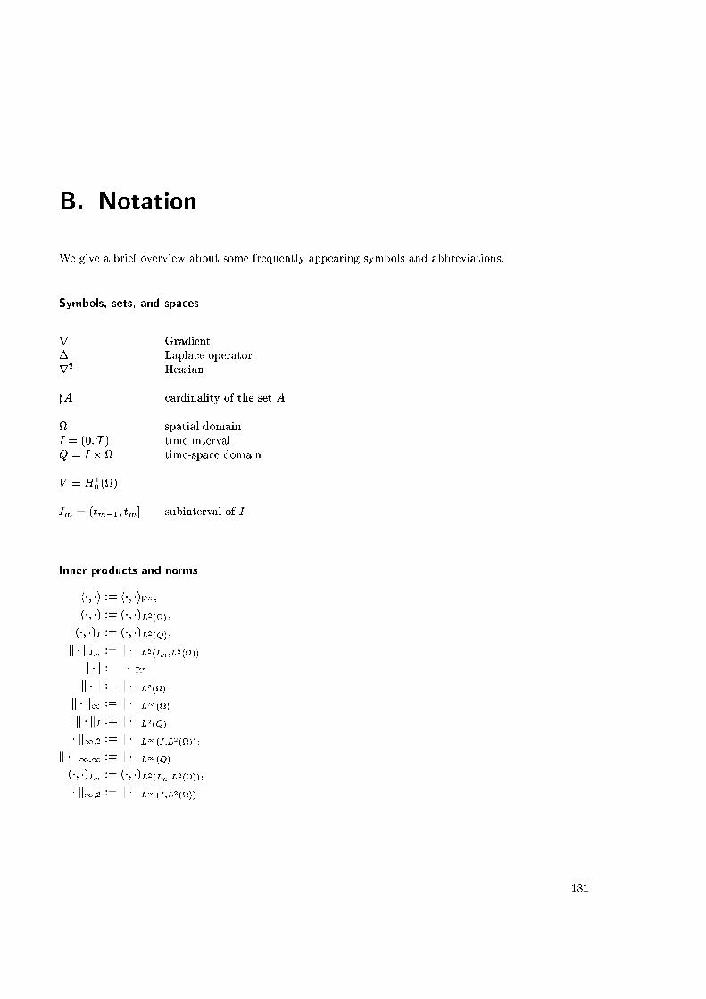
B. Notation
We give a brief overview about some frequently appearing symbols and abbreviations.
Symbols, sets, and spaces
r Gradient� Laplace operatorr2 Hessian
]A cardinality of the set A
spatial domainI = (0; T ) time intervalQ = I � time-space domain
V = H10 ()
Im = (tm�1; tm] subinterval of I
Inner products and norms
h�; �i := h�; �iRn ;(�; �) := (�; �)L2();(�; �)I := (�; �)L2(Q);
k � kIm := k � kL2(Im;L2())j � j := j � jRnk � k := k � kL2()
k � k1 := k � kL1()
k � kI := k � kL2(Q)
k � k1;2 := k � kL1(I;L2());
k � k1;1 := k � kL1(Q)
(�; �)Im := (�; �)L2(Im;L2());k � k1;2 := k � kL1(I;L2())
181

Bibliography
[1] R. A. Adams. Sobolev Spaces, volume 65 of Pure and applied mathematics: a series of monographsand textbooks. Academic Press, New York { San Francisco { London, 1975.
[2] J.-J. Alibert and J.-P. Raymond. Boundary control of semilinear elliptic equations with discon-tinuous leading coe�cients and unbounded controls. Numer. Funct. Anal. and Optimization, 3and 4:235{250, 1997.
[3] H. W. Alt. Lineare Funktionalanalysis. Springer-Verlag, Berlin, 1999.
[4] W. Alt. On the approximation of in�nite optimization problems with an application to optimalcontrol problems. Appl. Math. Opt., 12:15{27, 1984.
[5] W. Alt. The Lagrange-Newton method for in�nite dimensional optimization problems. NumericalFunctional Analysis and Optimization, 11:201{224, 1990.
[6] W. Alt. Nichtlineare Optimierung. Vieweg, Braunschweig, 2002.
[7] W. Alt, R. Griesse, N. Metla, and A. R�osch. Lipschitz stability for elliptic optimal control problemswith mixed control-state constraints. Optimization, 59:833{849, 2010.
[8] N. Arada, E. Casas, and F. Tr�oltzsch. Error estimates for the numerical approximation of asemilinear elliptic control problem. Computational Optimization and Applications, 23:201{229,2002.
[9] N. Arada and J. P. Raymond. Dirichlet boundary control of semilinear parabolic equations. Part1: Problems with no state constraints. Appl. Math. Optim., 45:125{143, 2002.
[10] M. Bergounioux, M. Haddou, M. Hinterm�uller, and K. Kunisch. A comparison of a Moreau-Yosida-based active set strategy and interior point methods for constrained optimal control prob-lems. SIAM J. Optimization, 11:495{521, 2000.
[11] M. Bergounioux and K. Kunisch. On the structure of the Lagrange multipliers for state-constrained optimal control problems. Systems and Control Letters, 48:16{176, 2002.
[12] M. Bergounioux and K. Kunisch. Primal-dual active set strategy for state-constrained optimalcontrol problems. Computational Optimization and Applications, 22:193{224, 2002.
[13] M. Bergounioux and F. Tr�oltzsch. Optimal control of linear bottleneck problems. ESAIM COCV,3:235{250, 1998.
[14] M. Bergounioux and F. Tr�oltzsch. Optimal control of semilinear parabolic equations with state-constraints of bottleneck type. ESAIM COCV, 4:595{608, 1999.
183
184 Bibliography
[15] J. T. Betts and S. L. Campbell. Discretize then Optimize. In D. R. Ferguson and T. J. Peters,editors,Mathematics in Industry: Challenges and Frontiers A Process View: Practice and Theory.SIAM Publications, Philadelphia, 2005.
[16] F. Bonnans and A. Shapiro. Perturbation analysis of optimization problems. Springer, New York,2000.
[17] E. Casas. Control of an elliptic problem with pointwise state constraints. SIAM J. Control andOptimization, 4:1309{1322, 1986.
[18] E. Casas. Boundary control of semilinear elliptic equations with pointwise state constraints. SIAMJ. Control and Optimization, 31:993{1006, 1993.
[19] E. Casas. Pontryagin's principle for state-constrained boundary control problems of semilinearparabolic equations. SIAM J. Control and Optimization, 35:1297{1327, 1997.
[20] E. Casas. Error estimates for the numerical approximation of semilinear elliptic control problemswith �nitely many state constraints. ESAIM: Control, Optimization and Calculus of Variations,31:345{374, 2002.
[21] E. Casas. Using piecewise linear functions in the numerical approximation of semilinear ellipticcontrol problems. Advances in Computational Mathematics, 26:137{153, 2007.
[22] E. Casas, J. de los Reyes, and F. Tr�oltzsch. Su�cient second-order optimality conditions forsemilinear control problems with pointwise state constraints. SIAM J. on Optimization, 19(2):616{643, 2008.
[23] E. Casas and M. Mateos. Uniform convergence of the FEM. Applications to state constrainedcontrol problems. J. of Computational and Applied Mathematics, 21:67{100, 2002.
[24] E. Casas and M. Mateos. Error estimates for the numerical approximation of boundary semilin-ear elliptic control problems. Continuous piecewise linear approximations. In Systems, control,modeling and optimization, volume 202 of IFIP Int. Fed. Inf. Process., pages 91{101. Springer,New York, 2006.
[25] E. Casas, M. Mateos, and F. Tr�oltzsch. Error estimates for the numerical approximation ofboundary semilinear elliptic control problems. Computational Optimization and Applications,31:193{220, 2005.
[26] E. Casas and F. Tr�oltzsch. Error estimates for the �nite-element approximation of a semilinearelliptic control problem. Control and Cybernetics, 31:695{712, 2002.
[27] E. Casas and F. Tr�oltzsch. Error estimates for linear-quadratic elliptic control problems. InAnalysis and Optimization of Di�erential Systems. Kluwer Academic Publishers, 2003.
[28] E. Casas, F. Tr�oltzsch, and A. Unger. Second order su�cient optimality conditions for a nonlinearelliptic control problem. J. for Analysis and its Applications, 15:687{707, 1996.
[29] E. Casas, F. Tr�oltzsch, and A. Unger. Second order su�cient optimality conditions for some state-constrained control problems of semilinear elliptic equations. SIAM Control Optim., 38:1369{1391,2000.
Bibliography 185
[30] S. Cherednichenko, K. Krumbiegel, and A. R�osch. Error estimates for the Lavrentiev regulariza-tion of elliptic optimal control problems. Inverse Problems, 24(5):055003, 2008.
[31] S. Cherednichenko and A. R�osch. Error estimates for the regularization of optimal control prob-lems with pointwise control and state constraints. ZAA, 27(2):195{212, 2008.
[32] S. Cherednichenko and A. R�osch. Error estimates for the discretization of elliptic control problemswith pointwise control and state constraints. COAP, 44:27{55, 2009.
[33] K. Chrysa�nos. Convergence of discontinuous Galerkin approximations of an optimal controlproblem associated to semilinear parabolic pde's. ESAIM: M2AN, 44:189{206, 2010.
[34] P. Ciarlet. The Finite Element Method for Elliptic Problems. North-Holland, Amsterdam, 1978.
[35] P. Cl�ement. Approximation by �nite element functions using local regularization. Revue Franc.Automat. Inform. Rech. Operat., 9(2):77{84, 1975.
[36] J. C. de los Reyes, P. Merino, J. Rehberg, and F. Tr�oltzsch. Optimality conditions for state-constrained PDE control problems with �nite-dimensional control space. Control Cybern., 37:5{38, 2008.
[37] K. Deckelnick, A. G�unther, and M. Hinze. Finite element approximation of Dirichlet boundarycontrol for elliptic PDEs on two- and three-dimensional curved domains. SIAM Control Optim.,48(4):2798{2819, 2009.
[38] K. Deckelnick and M. Hinze. Convergence of a �nite element approximation to a state constrainedelliptic control problem. SIAM J. Numer. Anal., 45:1937{1953, 2007.
[39] K. Deckelnick and M. Hinze. Numerical analysis of a control and state constrained elliptic controlproblem with piecewise constant control approximations. In K. Kunisch, G. Of, and O. Steinbach,editors, Proceedings of ENUMATH 2007, the 7th European Conference on Numerical Mathematicsand Advanced Applications, Heidelberg, September 2007 2008. Springer.
[40] K. Deckelnick and M. Hinze. Variational discretization of parabolic control problems in thepresence of pointwise state constraints. J. Comp. Math., 29:1{16, 2011.
[41] P. Deu hardt, M. Seebass, D. Stalling, R. Beck, and H.-C. Hege. Hyperthermia treatment plan-ning in clinical cancer therapy: Modelling, simulation, and visualization. In A. Sydow, editor,Computational Physics, Chemistry and Biology, pages 9{17. Wissenschaft und Technik- Verlag,1997.
[42] A. L. Dontchev. Local analysis of a Newton{type method based on partial linearization. InJ. Renegar, M. Shub, and S. Smale, editors, Proceedings of the AMS{SIAM Summer Seminar inApplied Mathematics on Mathematics of Numerical Analysis: Real Number Algorithms, volume 32of AMS Lectures in Appl. Math., pages 295{306, 1996.
[43] K. Eppler and F. Tr�oltzsch. Fast optimization methods in the selective cooling of steel. InM. Gr�otschel, S. O. Krumke, and J. Rambau, editors, Online Optimization of Large Scale Systems,pages 185{204. Springer, 2001.
186 Bibliography
[44] K. Eriksson, D. Estep, P. Hansbo, and C. Johnson. Computational Di�erential Equations. Cam-bridge Univ. Press, UK, 1996.
[45] K. Eriksson and C. Johnson. Adaptive �nite element methods for parabolic problems I: A linearmodel problem. SIAM J. Numer. Anal., 28(1):43{77, 1991.
[46] K. Eriksson and C. Johnson. Adaptive �nite element methods for parabolic problems II: Optimalerror estimats in L1L2 and L1L1. SIAM J. Numer. Anal., 32(3):706{740, 1995.
[47] K. Eriksson, C. Johnson, and V. Thom�ee. Time discretization of parabolic problems by thediscontinuous Galerkin method. M2AN Math. Model. Numer. Anal., 19:611{643, 1985.
[48] L. C. Evans. Partial Di�erential Equations. American Math. Society, Providence, Rhode Island,1998.
[49] R. S. Falk. Approximation of a class of optimal control problems with order of convergenceestimates. J. Math. Anal. Appl., 44:28{47, 1973.
[50] T. Geveci. On the approximation of the solution of an optimal control problem governed by anelliptic equation. R.A.I.R.O. Analyse num�erique/ Numerical Analysis, 13:313{328, 1979.
[51] D. Gilbarg and N. Trudinger. Elliptic Partial Di�erential Equations of Second Order. Springer,1977.
[52] H. Goldberg and F. Tr�oltzsch. Second order su�cient optimality conditions for a class of con-trol problems governed by non-linear integral equations with application to parabolic boundarycontrol. Optimization, 20:671{698, 1989.
[53] H. Goldberg and F. Tr�oltzsch. Second order su�cient optimality conditions for a class of non-linearparabolic boundary control problems. SIAM Control Optim., 31:1007{1025, 1993.
[54] H. Goldberg and F. Tr�oltzsch. On a Lagrange-Newton method for a nonlinear parabolic boundarycontrol problem. Optimization Methods and Software, 8(3):225{247, 1998.
[55] G. Gramlich, R. Hettich, and E. Sachs. Local convergence of SQP methods in semi-in�niteprogramming. SIAM J. Optim., 5:641{658, 1995.
[56] J. A. Griepentrog. Linear elliptic boundary value problems with non-smooth data: Campanatospaces of functionals. Math. Nachr., 243:19{42, 2002.
[57] J. A. Griepentrog. Maximal regularity for nonsmooth parabolic problems in Sobolev-Morreyspaces. Adv. Di�erential Eequations, 12:1031{1078, 2007.
[58] J. A. Griepentrog. Sobolev-Morrey spaces associated with evolution equations. Adv. Di�erentialEquations, 12:781{840, 2007.
[59] R. Griesse. Lipschitz stability of solutions to some state-constrained elliptic optimal controlproblems. Zeitschrift f�ur Analysis und ihre Anwendungen, 25(4):435{455, 2006.
[60] R. Griesse, N. Metla, and A. R�osch. Convergence analysis of the SQP method for nonlinearmixed-constrained elliptic optimal control problems. ZAMM, 88(10):776{792, 2008.
Bibliography 187
[61] R. Griesse, N. Metla, and A. R�osch. Local quadratic convergence of SQP for elliptic optimalcontrol problems with mixed control-state constraints. Control Cybern., 39(3):717{738, 2010.
[62] P. Grisvard. Elliptic Problems in Nonsmooth Domains. Pitman, Boston, 1985.
[63] A. G�unter and M. Hinze. Elliptic control problems with gradient constraints - variational discreteversus piecewise constant controls. Comput. Optim. Appl., appeared online:DOI: 10.1007/s10589{009{9308{8, 2009.
[64] M. D. Gunzburger. Perspectives in ow control and optimization. SIAM, 2003.
[65] M. Hinterm�uller and M. Hinze. Moreau-yosida regularization in state constrained elliptic controlproblems: Error estimates and parameter adjustment. SIAM J. on Numerical Analysis, 47:1666{1683, 2009.
[66] M. Hinterm�uller, K. Ito, and K. Kunisch. The primal-dual active set strategy as a semismoothNewton method. SIAM J. Optim., 13:865{888, 2003.
[67] M. Hinterm�uller and K. Kunisch. Path-following methods for a class of constrained minimizationproblems in function space. SIAM J. on Optimization, 17:159{187, 2006.
[68] M. Hinterm�uller and K. Kunisch. PDE-constrained optimization subject to pointwise constraintson the control, the state, and its derivative. SIAM J. Optim., 20(3):1133{1156, 2009.
[69] M. Hinterm�uller, F. Tr�oltzsch, and I. Yousept. Mesh-independence of semismooth Newton meth-ods for Lavrentiev-regularized state constrained nonlinear optimal control problems. NumerischeMathematik, 108(4):571{603, 2008.
[70] M. Hinterm�uller and I. Yousept. A sensitivity-based extrapolation technique for the numericalsolution of state-constrained optimal control problems. ESAIM COCV, 16(3):503{522, 2010.
[71] M. Hinze. A variational discretization concept in control constrained optimization: the linear-quadratic case. J. Computational Optimization and Applications, 30:45{63, 2005.
[72] M. Hinze and C. Meyer. Stability of semilinear elliptic optimal control problems with pointwisestate constraints. Technical Report 1236, WIAS, 2007.
[73] M. Hinze and C. Meyer. Variational discretization of Lavrentiev-regularized state constrainedelliptic optimal control problems. Computational Optimization and Applications, 46:487{510,2010.
[74] M. Hinze, R. Pinnau, M. Ulbrich, and S. Ulbrich. Optimization with pde constraints. MathematicalModelling: Theory and Applications. Springer, 2008.
[75] M. Hinze and A. Schiela. Discretization of interior point methods for state constrained ellipticoptimal control problems: Optimal error estimates and parameter adjustment. COAP, publishedonline, DOI: 10.1007/s10589-009-9278-x, 2009.
[76] D. H�omberg. A mathematical model for induction hardening including mechanical e�ects. Non-linear Anal. Real World Appl., 5:55{90, 2004.
188 Bibliography
[77] M. Huth and R. Tichatschke. A hybrid method for semi-in�nite programming problems. Opera-tions research, Proc. 14th Symp. Ulm/FRG 1989,Methods Oper. Res., 62:79{90, 1990.
[78] K. Ito and K. Kunisch. Semi-smooth Newton methods for state-constrained optimal controlproblems. Systems and Control Letters, 50:221{228, 2003.
[79] N. Josephy. Newton's method for generalized equations. Technical Summary Report 1965, Math-ematics Research Center, University of Wisconsin, Madison, WI, 1979.
[80] D. Kinderleher and G. Stampacchia. An introduction to variational inequalities and their appli-cations. Pure and applied mathematics: a series of monographs and textbooks. Academic Press,New York { San Francisco { London, 1980.
[81] M. A. Krasnoselskii, P. P. Zabreiko, E. I. Pustylnik, and P. E. Sbolevskii. Integral operators inspaces of summable functions. Noordho� International Publishing, Leyden, 1976.
[82] A. Kr�oner and B. Vexler. A priori error estimates for elliptic optimal control problems withbilinear state equation. J. Comp. Appl. Math., 230(2):781{802, 2009.
[83] K. Krumbiegel, I. Neitzel, and A. R�osch. Regularization for semilinear elliptic optimal controlproblems with pointwise state and control constraints. Comput. Optim. Appl., online �rst(6):DOI:10.1007/s10589{010{9357{z, 2010.
[84] K. Krumbiegel, I. Neitzel, and A. R�osch. Su�cient optimality for the moreau{yosida-type reg-ularization concept applied to semilinear elliptic optimal control problems with pointwise stateconstraints. Annals of the Academy of Romanian Scientists, Series on Mathematics and its Ap-plications, 2(2):222{246, 2010.
[85] K. Krumbiegel and A. R�osch. A virtual control concept for state constrained optimal controlproblems. COAP, 43(2):213{233, 2009.
[86] O. A. Ladyzhenskaya, V. A. Solonnikov, and N. N. Ural'ceva. Linear and Quasilinear Equationsof Parabolic Type. American Math. Society, Providence, R.I., 1968.
[87] I. Lasiecka and K. Malanowski. On discrete-time Ritz-Galerkin approximation of control con-strained optimal control problems for parabolic systems. Control Cybern., 7:21{36, 1978.
[88] M. M. Lavrentiev. Some improperly posed problems of mathematical physis. Springer, 1967.
[89] J. L. Lions. Quelques m�ethodes de r�esolution des probl�emes aux limites non lin�eaires. DunodGauthier{Villars, 1969.
[90] J. L. Lions. Optimal Control of Systems Governed by Partial Di�erential Equations. Springer-Verlag, Berlin, 1971.
[91] D. Luenberger. Optimization by Vector Space Methods. Wiley, New York, 1969.
[92] K. Malanowski. Convergence of approximations vs. regularity of solutions for convex, control{constrained optimal control problems. Applied Math. Optimization, 8:69{95, 1981.
Bibliography 189
[93] K. Malanowski. Stability and sensitivity analysis for optimal control problems with control{stateconstraints. Dissertationes Mathematicae (Rozprawy Matematyczne), 394:51 pp, 2001.
[94] K. Malanowski and F. Tr�oltzsch. Lipschitz stability of solutions to parametric optimal control forparabolic equations. Journal of Analysis and its Applications, 18(2):469{489, 1999.
[95] K. Malanowski and F. Tr�oltzsch. Lipschitz stability of solutions to parametric optimal control ofelliptic equations. Control Cybern., 29:237{256, 2000.
[96] M. Mateos. Problemas de Control �Optimo Gobernados por Ecuaciones Semilineales con Restric-ciones de Tipo Integral sobre el Gradiente del Estado. PhD thesis, Universidad de Cantabria,2000.
[97] The Mathworks. Optimization Toolbox User's guide. www.mathworks.com/help/toolbox/optim/.
[98] R. S. McNight and W. E. Bosarge, Jr. The Ritz-Galerkin procedure for parabolic control problems.SIAM J. Control, 11:510{524, 1973.
[99] D. Meidner. Adaptive Space-Time Finite Element Methods for Optimization Problems Governedby Nonlinear Parabolic Systems. PhD thesis, Ruprecht-Karls-Universit�at Heidelberg, 2008.
[100] D. Meidner, R. Rannacher, and B. Vexler. A priori error estimates for �nite element discretizationsof parabolic optimization problems with pointwise state constraints in time. Technical Report099, SPP1253, 2010.
[101] D. Meidner and B. Vexler. A priori error estimates for space-time �nite element discretization ofparabolic optimal control problems Part I: Problems without control constraints. SIAM ControlOptim., 47(3):1150{1177, 2008.
[102] D. Meidner and B. Vexler. A priori error estimates for space-time �nite element discretizationof parabolic optimal control problems Part II: Problems with control constraints. SIAM ControlOptim., 47(3):1301{1329, 2008.
[103] D. Meidner and B. Vexler. A priori error analysis of the petrov galerkin crank nicolson schemefor parabolic optimal control problems. Technical Report 109, SPP1253, 2010.
[104] P. Merino, I. Neitzel, and F. Tr�oltzsch. Error estimates for the �nite element discretization ofsemi-in�nite elliptic optimal control problems. Discussiones Mathematicae Di�erential Inclusions,Control and Optimization, 30(2):221{236, 2010.
[105] P. Merino, I. Neitzel, and F. Tr�oltzsch. On linear-quadratic elliptic optimal control problemsof semi-in�nite type. Applicable Analysis., published online:DOI 10.1080/00036811.2010.489187,2010.
[106] P. Merino, F. Tr�oltzsch, and B. Vexler. Error Estimates for the Finite Element Approximationof a Semilinear Elliptic Control Problem with State Constraints and Finite Dimensional ControlSpace. ESAIM:Mathematical Modelling and Numerical Analysis, 44:167{188, 2010.
[107] C. Meyer. Error estimates for the �nite-element approximation of an elliptic control problem withpointwise state and control constraints. Control Cybern., 37:51{85, 2008.
190 Bibliography
[108] C. Meyer, U. Pr�ufert, and F. Tr�oltzsch. On two numerical methods for state-constrained ellipticcontrol problems. Optimization Methods and Software, 22(6):871{899, 2007.
[109] C. Meyer and A. R�osch. Superconvergence properties of optimal control problems. SIAM J.Control and Optimization, 43:970{985, 2004.
[110] C. Meyer, A. R�osch, and F. Tr�oltzsch. Optimal control of PDEs with regularized pointwise stateconstraints. Computational Optimization and Applications, 33(2003-14):209{228, 2006.
[111] C. Meyer and F. Tr�oltzsch. On an elliptic optimal control problem with pointwise mixed control-state constraints. In A. Seeger, editor, Recent Advances in Optimization. Proceedings of the 12thFrench-German-Spanish Conference on Optimization held in Avignon, September 20-24, 2004,Lectures Notes in Economics and Mathematical Systems. Springer-Verlag, 2005.
[112] C. Meyer and I. Yousept. Regularization of state-constrained elliptic optimal control problems withnonlocal radiation interface conditions. Computational Optimization and Applications., 44:734{755, 2009.
[113] J. Ne�cas. Les M�ethodes Directes en Th�eorie des Equationes Elliptiques. Academia, Praque, 1967.
[114] I. Neitzel and F. Tr�oltzsch. On convergence of Lavrentiev regularization for semilinear parabolicoptimal control problems with pointwise control and state constraints. Proc. Appl. Math. Mech.,8(1):10865{10866, 2008.
[115] I. Neitzel and F. Tr�oltzsch. On convergence of regularization methods for nonlinear parabolicoptimal control problems with control and state constraints. Control and Cybernetics, 37(4):1013{1043, 2008.
[116] I. Neitzel and F. Tr�oltzsch. On regularization methods for the numerical solution of paraboliccontrol problems with pointwise state constraints. ESAIM Control, Optimisation and Calculus ofVariations, 15(2):426{453, 2009.
[117] I. Neitzel and F. Tr�oltzsch. Numerical analysis of state-constrained optimal control problems forPDEs. to appear in SPP1253 theme issue, 2010.
[118] I. Neitzel and B. Vexler. A priori error estimates for space-time �nite element discretization ofsemilinear parabolic optimal control problems. Technical Report 107, SPP1253, 2010. submittedto Numerische Mathematik.
[119] C. Ortner and W. Wollner. A priori error estimates for optimal control problems with pointwiseconstraints on the gradient of the state. Technical Report SPP1253-071, SPP1253, 2009.
[120] U. Pr�ufert and F. Tr�oltzsch. An interior point method for a parabolic optimal control problemwith regularized pointwise state constraints. ZAMM, 87(8{9):564{589, 2007.
[121] U. Pr�ufert, F. Tr�oltzsch, and M. Weiser. The convergence of an interior point method for anelliptic control problem with mixed control-state constraints. Comput. Optim. Appl., 39(2):183{218, March 2008.
[122] R. Rannacher and B. Vexler. A priori error estimates for the �nite element discretization of

Bibliography 191
elliptic parameter identi�cation problems with pointwise measurements. SIAM Control Optim.,44:1844{1863, 2005.
[123] J. Raymond and F. Tr�oltzsch. Second order su�cient optimality conditions for nonlinear paraboliccontrol problems with state constraints. Discrete Contin. Dyn. Syst., 6:431{450, 2000.
[124] J.-P. Raymond and H. Zidani. Pontryagin's principle for state-constrained control problems gov-erned by parabolic equations with unbounded controls. SIAM J. Control and Optimization,36:1853{1879, 1998.
[125] J.-P. Raymond and H. Zidani. Hamiltonian Pontryagin's Principles for control Problems governedby Semilinear Parabolic Equations. Applied Mathematics and Optimization, 39:143{177, 1999.
[126] R. Reemtsen and J.-J. R�uckmann (Eds.). Semi-In�nite Programming. Kluwer Academic Publish-ers, Boston, 1998.
[127] S. Robinson. Strongly regular generalized equations. Mathematics of Operation Research, 5:43{62,1980.
[128] A. R�osch. Error estimates for linear-quadratic control problems with control constraints. TechnicalReport 740-2002, TU Berlin, 2002.
[129] A. R�osch. Error estimates for parabolic optimal control problems with control constraints. Z. f�urAnalysis und ihre Anwendungen (ZAA), 23:353{376, 2004.
[130] A. R�osch. Error estimates for linear-quadratic control problems with control constraints. Opti-mization Methods and Software, 21, No. 1:121{134, 2006.
[131] A. R�osch and F. Tr�oltzsch. Su�cient second order optimality conditions for a parabolic optimalcontrol problem with pointwise state constraints. SIAM Control Optim., 42(1):138{154, 2003.
[132] A. R�osch and F. Tr�oltzsch. Existence of regular Lagrange multipliers for a nonlinear elliptic opti-mal control problem with pointwise control-state constraints. SIAM J. Control and Optimization,45:548{564, 2006.
[133] A. R�osch and F. Tr�oltzsch. Su�cient second-order optimality conditions for an elliptic optimalcontrol problem with pointwise control-state constraints. SIAM J. on Optimization, 17(3):776{794, 2006.
[134] A. R�osch and F. Tr�oltzsch. On regularity of solutions and Lagrange multipliers of optimal controlproblems for semilinear equations with mixed pointwise control-state constraints. SIAM J. Controland Optimization, 46(3):1098{1115, 2007.
[135] A. Schiela. Barrier methods for optimal control problems with state constraints. SIAM J. onOptimization, 20:1002{1031, 2009.
[136] G. Still. Discretization in semi-in�nite programming: the rate of convergence. MathematicalProgramming. A Publication of the Mathematical Programming Society, 91:53{69, 2001.
[137] G. Still. Generalized semi-in�nite programming: Numerical aspects. Optimization, 49:223{242,2001.
192 Bibliography
[138] V. Thom�ee. Galerkin Finite Element Methods for Parabolic Problems, volume 1054 of LectureNotes in Mathematics. Springer, 1984.
[139] H. Triebel. Interpolation Theory, Function Spaces, Di�erential Operators. North-Holland, Ams-terdam, New York, Oxford, 1978.
[140] F. Tr�oltzsch. On the Lagrange-Newton-SQP method for the optimal control of semilinear parabolicequations. SIAM Control Optim., 38:294{312, 1999.
[141] F. Tr�oltzsch. Lipschitz stability of solutions of linear-quadratic parabolic control problems withrespect to perturbations. Dyn. Contin. Discrete Impulsive Syst., 7:289{306, 2000.
[142] F. Tr�oltzsch. Regular Lagrange multipliers for problems with pointwise mixed control-state con-straints. SIAM J. Optimization, 15(2):616{634, 2005.
[143] F. Tr�oltzsch. On Finite Element error estimates for optimal control problems with elliptic PDEs.In I. Lirkov, S. Margenov, and J. Wasniewski, editors, Large Scale Scienti�c Computing, volume5910 of Lecture Notes in Computer Science, pages 40{53. Springer, 2010.
[144] F. Tr�oltzsch. Optimal Control of Partial Di�erential Equations: Theory, Methods and Applica-tions. AMS, Providence, 2010.
[145] F. Tr�oltzsch and I. Yousept. A regularization method for the numerical solution of elliptic bound-ary control problems with pointwise state constraints. COAP, 42(1):43{66, 2009.
[146] F. Tr�oltzsch and I. Yousept. Source representation strategy for optimal boundary control problemswith state constraints. Journal of Analysis and its Applications, 28(2):189{203, 2009.
[147] M. Ulbrich and S. Ulbrich. Primal-dual interior-point methods for PDE-constrained optimization.Math. Program., 117(1-2, Ser. B):435{485, 2009.
[148] A. Unger. Su�cient optimality conditions of second order and convergence of the SQP method forsemilinear elliptic boundary control problems. (Hinreichende Optimalit�atsbedingungen 2. Ordnungund Konvergenz des SQP-Verfahrens f�ur semilineare elliptische Randsteuerprobleme.). PhD thesis,Chemnitz: Technische Universit�at Chemnitz, Fakult�at Mathematik, 126 S. , 1997.
[149] F. G. V�azquez, J.-J. R�uckmann, O. Stein, and G. Still. Generalized semi-in�nite programming:a tutorial. J. Computational and Applied Mathematics, 217:394{419, 2008.
[150] R. Winther. Error Estimates for a Galerkin approximation of a parabolic control problem. Ann.Math. Pura Appl., 117(4):173{206, 1978.
[151] J. Wloka. Partielle Di�erentialgleichungen. Teubner-Verlag, Leipzig, 1982.
[152] I. Yousept. Optimal control of partial di�erential equations involving pointwise state constraints.PhD thesis, Technische Universit�at Berlin, 2008.
[153] J. Zowe and S. Kurcyusz. Regularity and stability for the mathematical programming problemin Banach spaces. Appl. Math. Optimization, 5:49{62, 1979.