European Journal of Mechanics B/Fluids ( ) –

Contents lists available at ScienceDirect

European Journal of Mechanics B/Fluids

journal homepage: www.elsevier.com/locate/ejmflu

Numerical and experimental study of pressure-wave formationaround an underwater ventilated vehicle

Xiaoshi Zhang a, Cong Wang a,∗, David Wafula Wekesa a,b

a School of Astronautics, Harbin Institute of Technology, Harbin 150001, Chinab Department of Physics, Jomo Kenyatta University of Agriculture & Technology, Nairobi City, Kenya

a r t i c l e i n f o

Article history:

Received 6 January 2016

Received in revised form

23 June 2016

Accepted 23 January 2017

Available online xxxx

Keywords:

Cavitation

Turbulence

Ventilated cavitation flows

Re-entrant jet

Filter-based turbulence model

a b s t r a c t

The objective of this study was to understand better the ventilated cavitation flow structure around anunderwater ventilated vehicle. A high-speed camera system was used to observe the cavity evolutionof unsteady cavitation flow, and a dynamic pressure measurement system was used to measure theinstantaneous pressure during cavity growth. The numerical simulation is presented using the secondarydevelopment of computational fluid dynamics code CFXwith a filter-based turbulencemodel. The resultsindicate that the ventilated flow rate of the gas influences the development of ventilated cavitation, andthe pressure fluctuation is suppressed remarkably by the ventilated cavity evolution. The results alsoindicate that the proposedmethod can effectively capture the unsteady cavitation structure in accordancewith the quantitative features observed in the experiment. It can therefore be concluded that the pressurefluctuations are induced by the vortex because of its periodic shedding toward downstream. The vortexshedding causes changes in the pressure distribution on the vehicle surface. Some secondary pressureoscillations can be observed that are attributable to the shedding of secondary vortex structures near thevehicle surface. These findings provide an important basis for facilitating the better understanding of theunsteady ventilated cavitation flows.

© 2017 Elsevier Masson SAS. All rights reserved.

1. Introduction

Cavitation around the low-pressure region of an underwatervehicle is associated with the launching of a process of high-speed vehicle [1]. When a vehicle is exiting the water, thepressure fluctuations generated by the cavitation bubbles collapse,which has a great influence on the trajectory and vibration ofthe vehicle. The cavitation around an axisymmetric vehicle andhydrofoils was investigated in previous studies [2–4]. Scholarshave discovered a complex phenomenon, that is shock wavesand jets are produced when the cavitation bubble collapses. Thecollapses may damage the structures attributable to cavitationerosion.Mostwork has been done in recent years on this particularaspect. Rouse and McNown [5] conducted a series of experimentson the cavitation flows of an axisymmetric model. Vlasenko [6]investigated the hydrodynamics of axisymmetric bodiesmoving inwater in supercavitation flow regime. The shedding evolution ofventilated unsteady partial cavitation was observed in a launching

∗ Corresponding author.

E-mail address: hitzxs@gmail.com (C. Wang).

experiment [7]. De Lange [8] observed two-dimensional (2D)and three-dimensional (3D) cavities. The experimental resultsshowed that the formation of a re-entrant flow is the maincause of unsteadiness. A mechanism of cavity unsteadiness wascaused by a re-entrant flow at the end of the cavity [9–12].Unsteady cavitation was investigated by different methods suchas the light intensity comparison [13], double optical probetechnique [14], the ultrasonic ultrasonography and laser Dopplervelocimetry [15], and X-ray imaging [16,17]. Huang [18,19] andHu [20–22] used high-speed video to observe the cavitation flows,and the velocity fields in a water tunnel weremeasured by particleimage velocimetry for different cavitation conditions. A peak ofpressure fluctuations was observed at the cavity closure. Thepeak magnitude increased with an increase in the cavity length.Although the cavitation process may not be avoided, it is notalways an undesired phenomenon in fluid dynamics. During thepast decade, the researchers tried their best to minimize theundesired effects of cavitation and maximize the advantage ofcavitation. Ceccin [23] presented the recent advances of the use ofpartial and supercavities for drag reduction of underwater vehiclesand surface ships moving in a liquid.

To help improve the understanding of the complex structures ofcavitation flows, various numerical methods have been proposed.

http://dx.doi.org/10.1016/j.euromechflu.2017.01.011

0997-7546/© 2017 Elsevier Masson SAS. All rights reserved.

2 X. Zhang et al. / European Journal of Mechanics B/Fluids ( ) –

In the CFD framework for cavitation simulation, different kindsof two-phase flow approaches have been developed. A bubbletwo-phase flow model was developed by Kubota et al. [24] thatcan explain the interactions between cavitation and vortices.Singhal [25] provided a vapor mass fraction equation withpressure-dependent source terms to simulate cavitation flowsin hydrofoils and orifices. Moreover, Sighal [26] employed amathematical approach to derive a correlation for ‘‘full cavitationmodel’’ in which all the first-order effects were considered.Merkle [27] deployed a two-species adding compressibility effectequation to analyze the natural cavitation. Besides, Kunz [28]presented an implicit algorithm to compute the viscous two-phaseflows and applied the algorithm to different models. Lindau etal. [29] and Kim et al. [30] adopted the Kunz model to study theunsteady 3D features of the cavitation flows over axisymmetricmodels with hemispheric and blunt noses. Senocak and Shyy [31]employed the pressure-basedmethod for computing the turbulentsheet cavitation flows. A three-component model was proposedthat considered the gas ventilation for simulating the naturaland ventilated cavitation around an underwater vehicle [32,33].In the numerical modeling of cavitation flows, the turbulencemodel determines the unsteady behavior of cavitation flows. TheReynolds-averaged Navier–Stokes (RANS) turbulence model ismostly used for single phase; however, some modifications [34]are required to make it suitable for compressible two-phasemixture flows. To better capture the unsteady features, sheet/cloudcavitation structures on the hydrofoils and ventilated cavitationare simulated by a large eddy simulation model [35–37]. Thepresent work is a study of ventilation cavitation flow structureusing the filter-based turbulence model (FBM). The FBM throughunsteady simulations was assessed with the experimental data.The simulation results showed that the FBM could effectivelycapture the transient turbulence structures than that by thestandard RANS models [38]. The ventilated cavitation flow on gasleakage behavior and re-entrant jet dynamics were investigatedby combining numerical methods and experimental methods. Ahigh-speed video camerawas used to capture cavitation flows. Thenumerical simulation was performed by CFX with a free surfacemodel and the FBM [39].

Most researchers focus on the cavity shedding mechanisms ofunsteady cavitation flows over different models. However, fewpay attention to the evolution of cavity and pressure after thebeginning of ventilation over a vehicle. Therefore, in the presentstudy, the unsteady ventilated cavitation flows over an underwatervehicle is investigated by an experimental method combinedwith a numerical method. Emphasis is placed on the real-timechanges in cavity and pressure by experiment. The mechanismand flow structure in the unsteady ventilated cavitation are shownby numerical analysis to facilitate better understanding of theunsteady ventilated cavitation flows.

2. Description of numerical methods

2.1. Conservation of mass and momentum

In the mixture model of the multiphase flow, the governingcontinuity and momentum equations for a classical RANS and thehomogeneous mixture multiphase flow equation shown are asfollows:

∂ρm

∂t+

∂

ρmuj

∂xj= 0; (1)

∂(ρmui)

∂t+

∂(ρmuiuj)

∂xj= ρfi −

∂p

∂xi+

∂

∂xj

×

(µm + µt)

∂ui

∂xj+

∂uj

∂xi−

2

3

∂ui

∂xjδij

. (2)

Fig. 1. Computation domain and boundaries.

Fig. 2. Sketch of the test body’s position in the test section.

Fig. 3. Mesh generation around the vehicle surface.

The subscripts i, j, and k represent the axes directions of theaxes, u is the velocity, p is the mixture pressure, and µt is theturbulent viscosity [40]; the mixture density ρm and the mixturelaminar viscosity µm are defined as

ρm =

n

k=1

αkρk; µm =

n

k=1

αkµk (3)

where αk is the volume fraction of phase k, n is the number of

phases.

2.2. Filter-based turbulence model

The numerical simulation is presented by the secondarydevelopment of computational fluid dynamics code CFX by usingan FBM. The filter turbulence fields use a modified form of thestandard k − ε [41] turbulence model shown as follows:

∂(ρk)

∂t+

∂(ρuik)

∂xj= Pk − ρε +

∂

∂xj

µ +µt

σk

∂k

∂xj

; (4)

X. Zhang et al. / European Journal of Mechanics B/Fluids ( ) – 3

Fig. 4. Schematic of the water tunnel.

Fig. 5. Schematic of the test section.

∂(ρε)

∂t+

∂(ρujε)

∂xj= Cε1

ε

kPk − Cε2ρ

ε2

k+

∂

∂xj

×

µ +µt

σε

∂ε

∂xj

. (5)

In our model, however, the two turbulence fields representconditionally ensemble averaged and filtered values, facilitated bythe definition of the eddy viscosity, and in the limit of coarse filtersand slow transient flows, the standard k − ε turbulence model isrecovered. The turbulent energy production (Pt ) and the Reynolds

stress tensor terms (τij) are defined as

Pt = τij∂ui

∂xj; τij =

2

3ρmkδij − µT

∂ui

∂xj+

∂uj

∂xi

(6)

where Cε1 = 1.44, Cε2 = 1.92, σε = 1.3, and σk = 1.0. Theturbulent eddy viscosity is defined as

µt =Cµρk2

ε, Cµ = 0.09. (7)

Johansen [42] proposed a special filter to help reduce µt ; ifthe turbulent scales are smaller than the set filter size, they willnot be resolved. Specifically, the level of the turbulent viscosity iscorrected by comparing the turbulence length scale and the filtersize ∆, which is selected depending on the local meshing spacing

µt =Cµρk2

εF , Cµ = 0.09

F = Min

1, C3

∆ · ε

k3/2

, C3 = 1.0

(8)

when ∆ ≫ k3/2/ε, Eq. (8) yields µt = Cµρk2/ε, and we recover

the standard k−ε model when∆ ≪ k3/2ε andµt = Cµρ ·∆ ·k1/2.

2.3. Numerical set-up and description

Fig. 1 shows the shape of the vehicle and the computationaldomain. The rectangular cross-section has a height of 260 mmand a width of 260 mm. The diameter of the cylindrical partof the vehicles is D = 40 mm and the length of the vehicle

Fig. 6. Cross-section of the test body.

4 X. Zhang et al. / European Journal of Mechanics B/Fluids ( ) –

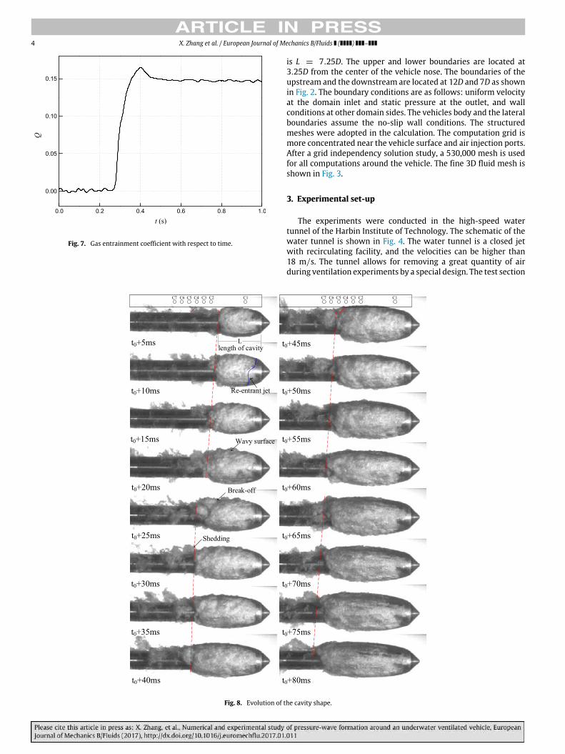
Fig. 7. Gas entrainment coefficient with respect to time.

is L = 7.25D. The upper and lower boundaries are located at

3.25D from the center of the vehicle nose. The boundaries of the

upstream and the downstream are located at 12D and 7D as shown

in Fig. 2. The boundary conditions are as follows: uniform velocity

at the domain inlet and static pressure at the outlet, and wall

conditions at other domain sides. The vehicles body and the lateral

boundaries assume the no-slip wall conditions. The structured

meshes were adopted in the calculation. The computation grid is

more concentrated near the vehicle surface and air injection ports.

After a grid independency solution study, a 530,000 mesh is used

for all computations around the vehicle. The fine 3D fluid mesh is

shown in Fig. 3.

3. Experimental set-up

The experiments were conducted in the high-speed water

tunnel of the Harbin Institute of Technology. The schematic of the

water tunnel is shown in Fig. 4. The water tunnel is a closed jet

with recirculating facility, and the velocities can be higher than

18 m/s. The tunnel allows for removing a great quantity of air

during ventilation experiments by a special design. The test section

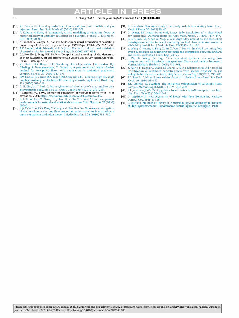
Fig. 8. Evolution of the cavity shape.

X. Zhang et al. / European Journal of Mechanics B/Fluids ( ) – 5

Fig. 9. Instantaneous pressure signals during cavity growth.

is a channel of 260× 260-mm rectangular cross-section and 1000-mm length with flat parallel sidewalls. The sidewalls of the testsection are equipped with transparent windows to perform visualobservations, and the air injection system is used as shown in Fig. 5.The main components of the test section are compressor, pressureregulating valve, and flow sensor. In this system, the ventilationpressure and the gas entrainment coefficient can be measured bythe flow sensors.

The test vehicle is mounted in the tunnel. The length of thetest body is L = 335 mm, and the diameter is D = 40 mm.A schematic of the test body is shown in Fig. 6. The surfacepressure at different locations on the model is also measured toaid the understanding of the observed flow physics. Seven CYG505transducer conditioners were embedded in the model to facilitatethe unsteady pressure measurements. The pressure transducers’locations are shown in Fig. 6. The cavitation flow around themodel was imaged with a Photron FASTCAM SA-X high-speedvideo camera. The velocity at the inlet of the test section was fixedat U0 = 8 m/s, and the pressure upstream of the vehicle at theinlet was 68.4 kPa. The camera and the data acquisition system aretriggered simultaneously.

4. Results and discussion

The unsteady cavitaton flows around the vehicle are investi-gated by both experimental and numerical methods. The gas en-trainment coefficient quantifies the gas required in the nondimen-sional form, which is given introduced by [43,44]

Q =Q̇

V∞D2n

where Q̇ is the volume flow rate of the injected gas. The values ofthe gas entrainment coefficient Q with respect to time are shownin Fig. 7. Thus, in the numerical simulation process, the air injectionis adjusted according to the dimensionless coefficient of the rate.

4.1. Evolution of cavitation pattern

To study the evolution of cavity and pressure after thebeginning of ventilation over a vehicle, the unsteady ventilatedcavitation flows over an underwater vehicle are investigated by anexperimental method.

The experimental evolution of the ventilated cavitation fromthe start of the ventilation until the ventilated cavity length stopsgrowing is shown in Fig. 8. The evolution of the cavity shape can bedescribed as follows. At the beginning of the cycle, the cavity formsand grows gradually after the vehicle is ventilated at t0 +5ms. Thecavity and re-entry jet influence each other. The adverse pressuregradient becomes strong and overcomes the momentum of theflow confined in the near-wall region, and the re-entrant flow thenforms at t0 + 10 ms. The re-entrant jet moves into the cavity afterits generation, and a partial re-entrant jet motion is observed. Theunsteady re-entrant jet impinges on the cavity boundaries, and thecavity boundaries become wavy as shown in Fig. 8 (t0 + 20 ms).A closer examination of the opaque regions reveals that the cavitysurface is not smooth in these areas. From t0+20 to t0+25ms, thecavity is cut by this reverse flow and forms sheet cavity, which islifted away from the vehicle surface leading to cavity break-off. Thebreak-off behavior becomes violent to cause the shedding cavity toroll up, and large cavity vortexes shed toward downstream. Fromt0 + 45 to t0 + 80 ms, the forefront of the transparent cavity formsa smooth interface. At this time, when the cavity length is half thevehicle, the increase in cavity length is more gradual and morefluctuating.

4.2. Wall-pressure fluctuations

Fig. 9 presents the instantaneous pressure signals during thecavity growth on the vehicle surface. The transducers on thesurface pass alternately from the noncavitating pressure to theventilated pressure, as shown in Fig. 8.

As the cavity grows, an increase in pressure fluctuations beforefalling to the ventilated pressure is revealed (see dashed lines inFig. 9 for C2–C5) when the cavity closure passes over the pressure

Fig. 10. Turbulence viscosity for different turbulence models.

6 X. Zhang et al. / European Journal of Mechanics B/Fluids ( ) –

Fig. 11. Development of cavitation.

transducers one after another. It is observed that the pressure

fluctuations are convected to the cavity wake. Then, a decrease

in the pressure fluctuations is observed before the pressure falls

to the ventilated pressure. The pressure decreases more gradually

with more fluctuation (see arrows in Fig. 9 for C4 and C5) when

the cavity length is half the vehicle. This corresponds to the re-

entrant jetmovement into the cavity. The pressure fluctuations are

detected by the pressure transducer on the vehicle surface.

4.3. Flow structure in the rear part of the cavity

The modeling of turbulence plays an important role in the

dynamics of the flow. An FBM originated from the k−ε turbulence

model [42] is first compared with the original k − ε turbulence

model [41] and assessed by the experimental data before being it

is used.

To study the differences of the turbulence between the original

k − ε model and the FBM of a single-phase flow, their turbulence

viscosities are compared. The turbulence viscosity around the

ventilated vehicle is shown in Fig. 10. For the original k− ε model,

a higher eddy viscosity is predicted than that for the FBM.

Fig. 11 shows the numerical and experimental unsteady cavity

evolution morphology around the vehicle at each stage. From

the numerical results of the 3D view, the cavity shapes are

extremely dissymmetrical along the vehicle. It indeed presents the

3D characteristics of the cavitation flows. The numerical results

are shown in both the 2D and 3D views. The results show that

the numerical predictions could capture the attached cavity with

the growing cavity. The cavity break-off, the horse-shoe vortex

structure with U-type shedding, and the secondary shedding are

Fig. 12. Pressure coefficient contours, C2–C6 for comparison with experimental

values.

in accordance with those observed in the experiment. Therefore, itis clear that the FBM can effectively capture the unsteady features.

To verify the computational results, the pressure fluctuationsalong the axisymmetric vehicle were compared with the exper-imental results as shown in Fig. 13. The monitor points indicatethe location of transducers as shown in Fig. 12. It was found thatthe computed pressure fluctuations qualitatively follow the exper-imentally observed trend, and a good quantitative agreement inthe cavitation number was observed. Although the differences be-tween the simulated and the experimental data are more substan-tial with decrease in pressure, the agreement is reasonable consid-ering the difficulties in experimental measurements and the com-pressibility effects of the numerical method.

X. Zhang et al. / European Journal of Mechanics B/Fluids ( ) – 7

100

90

80

70

Pre

ssu

re (

kP

a)

60

50

400.00 0.04 0.08 0.12

t (s)

0.16 0.20

100

90

80

70

P (

kP

a)

60

50

400.00 0.04 0.08 0.12

t (s)

0.16 0.20

100

90

80

70

P (

kP

a)

60

50

400.00 0.04 0.08 0.12

t (s)

0.16 0.20

100

90

80

70

P (

kP

a)

60

50

400.00 0.04 0.08 0.12

t (s)

0.16 0.20

Fig. 13. Pressure fluctuations on the vehicle surface at C2, C4, C5, and C6.

4.4. Unsteady cloud cavitating vortex and the induced pressure

In ventilated cavitation flows, we can find that the pressurewave of the vehicle is highly correlated with the evolution ofthe vortex structures. Fig. 15 shows the time evolutions of thepressure coefficient on the vehicle surfacewith growing cavity. Theinstantaneous vortex and the pressure coefficient distributions areadopted to describe the flow field. It is obvious that the unsteadyevolutions produced by the vortex shedding is themajor reason forinducing the pressure wave. The flow structures at representativetime instances (T1 = t0 + 15 ms, T2 = t0 + 25 ms, T3 =

t0 + 30 ms, and T4 = t0 + 35 ms) are shown in Fig. 14.The instantaneous velocity vectors and the air volume fractioncontours are used to investigate the unsteady vortex structures.To analyze the unsteady vortex better, pressure coefficient alongthe vehicle and vorticity are compared to show the hydrodynamicfluctuations. The relationship between the vortex structures andthe pressure is given in the following paragraph.

The cavity grows until the re-entry flow appears. When there-entry flow moves back to the front of the vehicle, the cavityseparates from the vehicle. Fig. 14 shows the flow structures nearthe vehicle surface at representative time instances. At T1 = t0 +

15 ms, a vortex on the surface rotating clockwise is defined as V1.Low pressure is distributed at the core of vortex V1 and a highpressure on the vehicle surface because of the adverse pressuregradient as shown in Fig. 15(a). At T2 = t0 + 25 ms, V1 leaves

the vehicle surface, and the shedding vortex induces a local highpressure at the vehicle surface. The high pressure (D) at the vehiclesurface and the low pressure (E) distributions at the core of vortexV1 sustain the adverse pressure gradient. It is necessary to form thesecond vortex structure rotating clockwise on the upper surface.The secondary vortex is defined as V2, which grows up because ofthe adverse pressure gradient. Then, vortexV1moves downstream.It can also be found that the low-pressure area at the core ofvortex V1 grows up. At T3 = t0 + 30 ms cycle, vortex V2 leavesthe cavity and vortex V3 grows up, which results in low-pressuredistributions on the vehicle surface. In addition, vortex V2 becomesweak. A high pressure can be observed at the core of vortex V2.When the re-entry flow moves back to the front of the vehicle,the cavity breaks. At T3 = t0 + 30 ms, the detached complexvortex structure can be observed near the rear part of the vehicle inFig. 14(c). It is consistent with the detached cloud cavity. Break-upof the vortex structure induces local high pressure. Then, the high-pressure region extends rapidly. At T4 = t0 + 35 ms, vortex V3begins to move downstream because of the high-speed main flowout of the boundary layer. Then, the pressure at the core of vortexV3 decreases.

5. Conclusions

In the present study, the evolution of cavity and pressure-wave formation of the ventilated vehicle was experimentally and

8 X. Zhang et al. / European Journal of Mechanics B/Fluids ( ) –

(a) T1 = t0 + 15 ms. (b) T2 = t0 + 25 ms.

(c) T3 = t0 + 30 ms.

(d) T4 = t0 + 35 ms.

Fig. 14. Instantaneous velocity vectors and air volume fraction contours.

numerically investigated. The mechanism of ventilated partialcavitation wasmade clear through the photo analysis based on thehigh-speed video observation and the frame difference method.An FBM model from the standard k − ε turbulence model wasproposed to analyze the details of unsteady ventilated cavitation.The following conclusions can be drawn.

(1) The experimental results show that the evolutions of venti-lated cavitation and the instantaneous pressure signals are ob-served during the cavity growth on the vehicle surface. It is ob-served that the pressure fluctuations are induced by the evo-

lution of cavity, shedding, and collapse of the cavitation. The

fluctuation pressure is located at the cavity closure depending

on the cavitation number.

(2) The FBMmodel is used to reduce the eddy viscosity due to the

lower filter function near the vehicle surface, which will lead

to very different cavity dynamic processes, as compared to the

experimental visualization results. In general, the predicted

cavity dynamic results obtained using the FBM model with

appropriate parameters are in good agreementwith those from

the experimental measurements and observations.

X. Zhang et al. / European Journal of Mechanics B/Fluids ( ) – 9

(a) T1 = t0 + 15 ms. (b) T2 = t0 + 25 ms.

(c) T3 = t0 + 30 ms. (d) T4 = t0 + 35 ms.

Fig. 15. Comparison between vorticity and distributions of the pressure coefficients along the vehicle surface.

(3) Vortex structure rotating clockwise sheds periodically intothe wake region, which leads to changes in the pressuredistribution on the vehicle surface. In addition, some secondarypressure oscillations can be observed,which are induced by theshedding of various vortex structures near the vehicle surface.

References

[1] J.R. Blake, D.C. Gibson, Cavitation bubbles near boundaries, Annu. Rev. FluidMech. 19 (1987) 99–123.

[2] R.E. Bensow, G. Bark, Implicit LES predictions of the cavitating flow on apropeller, ASME J. Fluids Eng. 132 (2010) 041302.

[3] O. Coutier Delgosha, F. Deniset, J.A. Astolfi, J.-B. Leroux, Numerical prediction ofcavitating flow on a two-dimensional symmetrical hydrofoil and comparisonto experiments, ASME J. Fluids Eng. 129 (2007) 279–292.

[4] F.M. Owis, A.H. Nayfeh, Numerical simulation of 3-D incompressible, multi-phase flows over cavitating projectiles, Eur. J. Mech. B Fluids 23 (2004)339–351.

[5] H. Rouse, J.S. McNown, Cavitation and pressure distribution: head forms atzero angle of yaw, 1948.

[6] Y.D. Vlasenko, Experimental investigation of supercavitation flow regimesat subsonic and transonic speeds, in: Fifth International Symposium onCavitation, Osaka, Japan, 2003.

[7] Y. Wang, C. Huang, T. Du, X. Wu, X. Fang, N. Liang, Y. Wei, Sheddingphenomenon of ventilated partial cavitation around an underwater projectile,Chin. Phys. Lett. 29 (2012) 014601.

[8] D. De Lange, G. De Bruin, Sheet cavitation and cloud cavitation, re-entrant jetand three-dimensionality, in: Fascination of Fluid Dynamics, Springer, 1998,pp. 91–114.

[9] Y. Kawanami, H. Kato, H. Yamaguchi, M. Tanimura, Y. Tagaya, Mechanism andcontrol of cloud cavitation, ASME J. Fluids Eng. 119 (1997) 788–794.

[10] J. Dang, G. Kuiper, Re-entrant jet modeling of partial cavity flow on two-dimensional hydrofoils, ASME J. Fluids Eng. 121 (1999) 773–780.

[11] R. Furness, S. Hutton, Experimental and theoretical studies of two-dimensionalfixed-type cavities, ASME J. Fluids Eng. 97 (1975) 515–521.

[12] T. Pham, F. Larrarte, D. Fruman, Investigation of unsteady sheet cavitation andcloud cavitation mechanisms, ASME J. Fluids Eng. 121 (1999) 289–296.

[13] H. Sayyaadi, Instability of the cavitating flow in a venturi reactor, Fluid Dyn.Res. 42 (2010) 055503.

[14] B. Stutz, J. Reboud, Experiments on unsteady cavitation, Exp. Fluids 22 (1997)191–198.

[15] M. Callenaere, J. Franc, J. Michel, M. Riondet, The cavitation instability inducedby the development of a re-entrant jet, J. Fluid Mech. 444 (2001) 223–256.

[16] M. Dular, I. Khlifa, S. Fuzier, M.A. Maiga, O. Coutier-Delgosha, Scale effect onunsteady cloud cavitation, Exp. Fluids 53 (2012) 1233–1250.

[17] B. Stutz, S. Legoupil, X-ray measurements within unsteady cavitation, Exp.Fluids 35 (2003) 130–138.

[18] B. Huang, Y.L. Young, G. Wang, W. Shyy, Combined experimental andcomputational investigation of unsteady structure of sheet/cloud cavitation,ASME J. Fluids Eng. 135 (2013) 071301.

[19] B. Huang, G. Wang, Experimental and numerical investigation of unsteadycavitating flows through a 2D hydrofoil, Sci. China Technol. Sci. 54 (2011)1801–1812.

[20] C. Hu, G. Wang, G. Chen, B. Huang, Three-dimensional unsteady cavitatingflows around an axisymmetric body with a blunt headform, J. Mech. Sci.Technol. 29 (2015) 1093–1101.

[21] C. Hu, G. Wang, B. Huang, Experimental investigation on cavitating flowshedding over an axisymmetric blunt body, Chin. J. Mech. Eng. 28 (2015)387–393.

[22] C. Hu, G. Wang, B. Huang, Y. Zhao, The inception cavitating flows over anaxisymmetric body with a blunt head-form, J. Hydrodyn. Ser. B 27 (2015)359–366.

10 X. Zhang et al. / European Journal of Mechanics B/Fluids ( ) –

[23] S.L. Ceccio, Friction drag reduction of external flows with bubble and gasinjection, Annu. Rev. Fluid Mech. 42 (2010) 183–203.

[24] A. Kubota, H. Kato, H. Yamaguchi, A new modelling of cavitating flows: Anumerical study of unsteady cavitation on a hydrofoil section, J. Fluid Mech.240 (1992) 59–96.

[25] A. Singhal, N. Vaidya, A. Leonard, Multi-dimensional simulation of cavitatingflows using a PDF model for phase change, ASME Paper FEDSM97-3272, 1997.

[26] A.K. Singhal, M.M. Athavale, H. Li, Y. Jiang, Mathematical basis and validationof the full cavitation model, J. Fluids Eng. 124 (2002) 617–624.

[27] C.L. Merkle, J. Feng, P.E. Buelow, Computational modeling of the dynamicsof sheet cavitation, in: 3rd International Symposium on Cavitation, Grenoble,France, 1998, pp. 47–54.

[28] R.F. Kunz, D.A. Boger, D.R. Stinebring, T.S. Chyczewski, J.W. Lindau, H.J.Gibeling, S. Venkateswaran, T. Govindan, A preconditioned Navier–Stokesmethod for two-phase flows with application to cavitation prediction,Comput. & Fluids 29 (2000) 849–875.

[29] J.W. Lindau, R.F. Kunz, D.A. Boger, D.R. Stinebring, H.J. Gibeling, High Reynoldsnumber, unsteady, multiphase CFDmodeling of cavitating flows, J. Fluids Eng.124 (2002) 607–616.

[30] D.-H. Kim,W.-G. Park, C.-M. Jung, Numerical simulation of cavitating flow pastaxisymmetric body, Int. J. Naval Archit. Ocean Eng. 4 (2012) 256–266.

[31] I. Senocak, W. Shyy, Numerical simulation of turbulent flows with sheetcavitation, 2001. http://resolver.caltech.edu/cav2001:sessionA7.002.

[32] B. Ji, X.-W. Luo, Y. Zhang, H.-J. Ran, H.-Y. Xu, Y.-L. Wu, A three-componentmodel suitable for natural and ventilated cavitation, Chin. Phys. Lett. 27 (2010)096401.

[33] B. Ji, X.-W. Luo, X.-X. Peng, Y. Zhang, Y.-L.Wu,H.-Y. Xu, Numerical investigationof the ventilated cavitating flow around an under-water vehicle based on athree-component cavitation model, J. Hydrodyn. Ser. B 22 (2010) 753–759.

[34] E. Goncalvès, Numerical study of unsteady turbulent cavitating flows, Eur. J.Mech. B Fluids 30 (2011) 26–40.

[35] G. Wang, M. Ostoja-Starzewski, Large Eddy simulation of a sheet/cloudcavitation on a NACA0015 hydrofoil, Appl. Math. Model. 31 (2007) 417–447.

[36] B. Ji, X. Luo, R.E. Arndt, X. Peng, Y. Wu, Large Eddy simulation and theoreticalinvestigations of the transient cavitating vortical flow structure around aNACA66 hydrofoil, Int. J. Multiph. Flow 68 (2015) 121–134.

[37] Y. Wang, C. Huang, X. Fang, X. Yu, X. Wu, T. Du, On the cloud cavitating flowover a submerged axisymmetric projectile and comparison between 2D RANSand 3D LES methods, J. Fluids Eng. (2015).

[38] J. Wu, G. Wang, W. Shyy, Time-dependent turbulent cavitating flowcomputations with interfacial transport and filter-based models, Internat. J.Numer. Methods Fluids 49 (2005) 739–761.

[39] Z. Wang, B. Huang, G. Wang, M. Zhang, F. Wang, Experimental and numericalinvestigation of ventilated cavitating flow with special emphasis on gasleakage behavior and re-entrant jet dynamics, Ocean Eng. 108 (2015) 191–201.

[40] R.S. Rogallo, P.Moin, Numerical simulation of turbulent flows, Annu. Rev. FluidMech. 16 (1984) 99–137.

[41] B.E. Launder, D. Spalding, The numerical computation of turbulent flows,Comput. Methods Appl. Math. 3 (1974) 269–289.

[42] S.T. Johansen, J. Wu,W. Shyy, Filter-based unsteady RANS computations, Int. J.Heat Fluid Flow 25 (2004) 10–21.

[43] G. Logvinovich, Hydrodynamics of Flows with Free Boundaries, NaukovaDumka, Kiev, 1969, p. 128.

[44] L. Epshtein, Methods of Theory of Dimensionality and Similarity in Problemsof Ship Hydromechanics, Sudostroenie Publishing House, Leningrad, 1970.