Numerical aspects of DFT

Jussi Enkovaara

CSC – IT Center for Science

Outline

● Real-space grids● Density mixing● Iterative solution of eigenproblem● Parallelization

Basis sets● Expand wave functions in a set of basis functions

● Turns (continuous) Kohn-Sham equations into discrete matrix equations

● Criteria for good basis set

― Accuracy― Numerical efficiency

Real-space grids● Wave functions, electron densities, and potentials are

represented on grids.● Single parameter, grid spacing h

h

● Accuracy of calculation can be improved systematically by decreasing the grid spacing

● Can work only with smooth wave functions

― Pseudopotential or PAW approximation is needed

Boundary conditions● Real-space description allows flexible

boundary conditions● Zero boundary conditions (finite systems)

― potential, charge density and wave functions are zeros at the cell boundaries

― possible to treat charged systems● Periodic boundary conditions (bulk systems)

― potential and charge are periodic― wave-functions obey Bloch boundary

conditions (k-points)● Boundary conditions can be mixed

― periodic in one dimension (wires)― periodic in two dimensions (surfaces)

Finite-differences

● Both the Poisson equation and kinetic energy contain the Laplacian which can be approximated with finite differences

● Accuracy depends on the order of the stencil N● Sparse matrix, storage not needed● Cost in operating to wave function is

proportional to the number of grid points

Hamiltonian in real-space ● Denoting grid points by G, the real-space

discretization of PAW Hamiltonian is

where LGG' is the finite-difference Laplacian

● Sparse matrix with large dimension, thus iterative techniques requiring only are used

Multigrid method● General framework for solving differential equations

with hierarchy of discretizations● Poisson equation

can be solved as

● Problem: critical slowing down for long wave length components of error

― solution: treat long wave length components on a coarser grid

― recursive restriction leads to the V-cycle

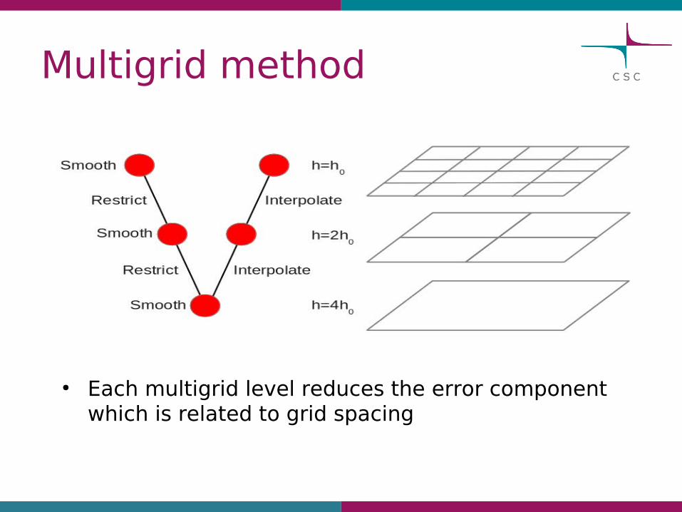
Multigrid method

● Each multigrid level reduces the error component which is related to grid spacing

Egg-box effect● Integrals involving localized functions centered on

an atom and functions spanning the whole simulation cell such as

are evaluated as sum over grid points

● The due to high frequency components in localized function, integral depends on the position of atom with respect to grid

Egg-box effect

● Problem: localization in real-space means delocalization in Fourier space and vice versa

● Fourier filtering is used for optimizing localization both in real and reciprocal spaces

Real-space method● Flexible boundary conditions● Systematic convergence● Uniform resolution – empty space expensive● Total energy is not variational with grid spacing● Egg-box effect● Efficient multigrid and iterative methods● Good parallelization prospects● Real-space program packages

― GPAW, Octopus, Parsec

Achieving self-consistency

Self-consistent cycle revisited

● In practice, the new electron density

is not used directly when calculating the effective potential for next iteration

● The new density is mixed with old density

Density mixing● Simplest approach: direct mixing

● Typically, small parameters are needed for the mixing to be stable

● Convergence can be slow● In spin-polarized systems, charge density and

magnetization density can be mixed separately

Pulay mixing● Mixing can be improved by using information from

previous iterations

● Pulay method assumes that the residual

depends linearly on the input density:

● Optimum set of αi is found by minimizing norm of the residual

where

Pulay mixing● Minimization of residual leads to

● Original Pulay method used only for obtaining the new density

● A weight factor can be included for covering the solution space more efficiently

● Parameters of Pulay mixing

― number of old densities to use― the weight factor

Charge sloshing● Small variation in input density can cause a large

change in output density

― Problem especially in large metallic systems― Convergence of SCF cycle can be slowed down

considerably● Charge sloshing is typically caused by the long range

changes in density● Filtering out long range changes in mixing can

reduce the effect of charge sloshing

Reducing charge sloshing● The long-wave length changes can be filtered out by

using a special metric when calculating the residuals

● In reciprocal space one can use a diagonal metric

● In real-space this metric is non-local, however it can approximated as

● The coefficient ci are chosen (with a weight factor w) as:

Broyden mixing● The SCF cycle can be interpreted as non-linear

problem

● Newton method:

● Broyden methods build successively approximation to inverse Jacobian J-1 using information from previous iterations

● Updates can be performed without explicit storage of (approximate) inverse Jacobian

Density mixing● Density mixing is needed for the SCF-cycle to

convergence● Different mixing schemes exist● Charge sloshing can be avoided by using suitable

metric● Optimum mixing parameters are highly system

dependent

Iterative solution of eigenproblem

● Determination of the effective potential from the input charge density is computationally simple

― Poisson equation can be tricky with some basis sets● The major task in SCF calculation is the

eigenproblem

● Well-established (dense) matrix diagonalization algorithms and libraries (LAPACK) can be used when basis size is modest

● If the basis is very large or the basis results in sparse matrix, iterative techniques may be advantageous

Iterative solution of eigenproblem

● Approximation for eigenvalue is obtained as

● All iterative methods are based on trial eigenfunction which is updated in each iteration

● Updates are normally based on the residual

● Iterative methods differ in how the residual is used● The full Hamiltonian matrix is not needed

― Only applying of the matrix to eigenfunction ― only O(N2) operations with sparse matrices

Preconditioning● Optimum update would be

● The residuals can be preconditioned by suitable approximations to the matrix inverse

● Preconditioned residuals can be obtained by solving approximately Poisson equation

● With plane wave basis a diagonal Teter preconditioner is often used

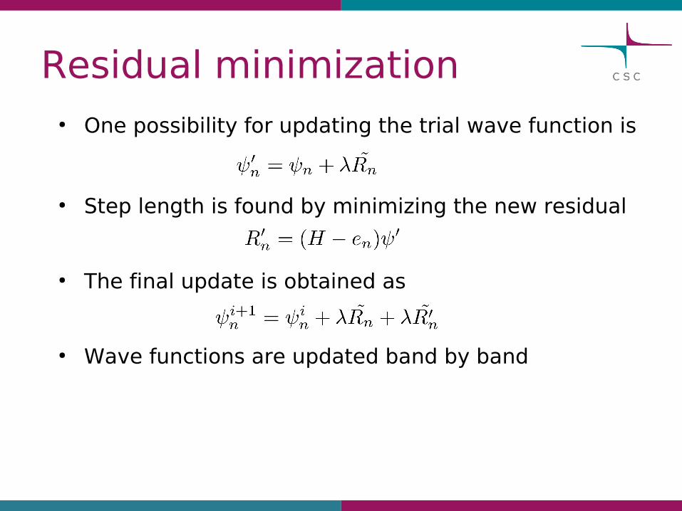
Residual minimization● One possibility for updating the trial wave function is

● Step length is found by minimizing the new residual

● The final update is obtained as

● Wave functions are updated band by band

Davidson method

● In simple Davidson method one first calculates the preconditioned residuals for each state

● One constructs then a vector from wave functions and preconditioned residuals

● Hamiltonian is then diagonalized in this basis and Nel lowest eigenvectors are used as new trial wave functions

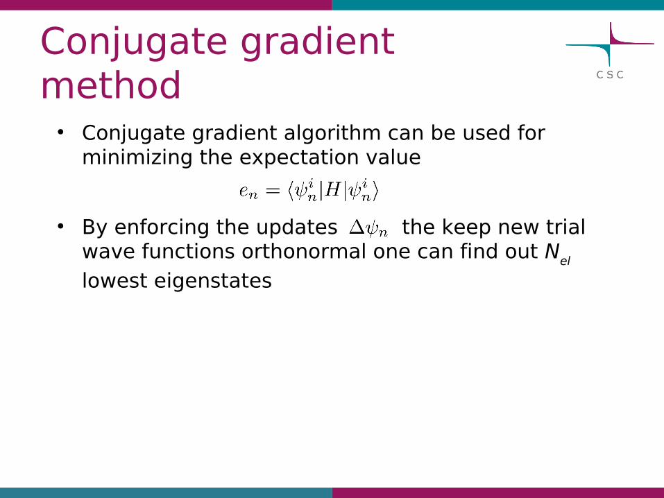
Conjugate gradient method

● Conjugate gradient algorithm can be used for minimizing the expectation value

● By enforcing the updates the keep new trial wave functions orthonormal one can find out Nel lowest eigenstates

Subspace diagonalization

● Both residual minimization and conjugate gradient algorithms calculate only arbitrary linear combination of Nel lowest eigenfunctions

● Hamiltonian can be diagonalized in the subspace of trial wave functions

● The Nel lowest eigenfunctions are obtained from subspace rotation:

Orthonormalization● After residual minimization the trial wave functions

are not orthonormal● Numerically efficient scheme for orthonormalization:

― Calculate overlap matrix

and determine its Cholesky decomposition L

― Orthonormal wave functions are obtained by multiplying with inverse Cholesky factor

Computational scaling of DFT calculation

● Poisson equation: O(Nb) – O(Nb log Nb)

● XC-potential

― semi-local functionals: O(Nb)

― EXX: O(Ne4 Nb)

● Direct solution of eigenproblem

― Construction of Hamiltonian: O(N2b)

― Diagonalization of Hamiltonian: O(N3b)

or● Iterative solution of eigenproblem

― Applying with Hamiltonian: O(Nel Nb) – O(Nel Nblog Nb)

― Subspace diagonalization: O(Nel3)

― Orthonormalization: O(Nel3)

Summary

● Density mixing is needed in SCF cycle● Iterative diagonalization schemes can be efficient with

sparse matrices● Computational scaling of DFT algorithm is

O(N3)― Direct eigensolvers: diagonalization dominates in large

systems― Iterative solvers: orthonormalization dominates in large

systems

Solving DFT equations in parallel

Parallel calculations

● Speedup in modern supercomputers is based on large number of CPUs

● In order to exploit available computing power, parallel computing is needed

● Parallel computing allows one― Solve problems faster― Solve bigger problems

Parallellization prospects in DFT

● Basis functions● k-points and spin● electronic states● Additional trivial parallelizations

― e.g. different atomic configurations or unit cells

Parallellization: k-points and spin

● Spin and k-points can be treated equivalently● Trivial parallelization● Limited scalability

― k-points only in (small) periodic systems― spin only in magnetic systems

Parallelization: basis

● Depends largely on the basis used● Plane waves : parallel FFT is challenging● Real-space grids: efficient domain decomposition

Finite difference LaplacianP1

P3 P4

P2PAW augmentation sphere

Parallelization: electronic states

● Orthonormalizations are complicated ― communication of all wave functions to all processes

― Can be implemented as pipeline with only nearest neighbour communication

Parallel scalability in practice

● Feasible amount of CPUs depends heavily on the studied system (number of atoms/electrons)

● Largest ground state DFT calculations use typically with few thousand CPU cores

● GPAW, real-space mode● 561 Au atoms, 6200

electrons● Blue Gene P, Argonne

Summary

● Parallelization is needed for fully exploiting modern computers

● DFT equations offer several parallelization levels― K-points, spin, basis, electronic states

● Optimum number of CPUs depend on the studied system

Overview of GPAW

GPAW● Implementation of projector augmented wave

method on― uniform real-space grids, atomic orbital basis,

plane waves● Density-functional theory and time-dependent DFT● Open source software licensed under GPL

― 20-30 developers in Europe and in USA

wiki.fysik.dtu.dk/gpaw 

J. J. Mortensen et al., Phys. Rev. B 71, 035109 (2005)

J. Enkovaara et al., J. Phys. Condens. Matter 22, 253202 (2010)

GPAW features● PAW-method: accurate description over the

whole periodic table● Total energies, forces, structural optimization

― analysis of electronic structure● Excited states, optical spectra

― Non-adiabatic electron-ion dynamics● Wide range of XC-potentials (thanks to libxc!)

― LDAs, GGAs, meta-GGAs, hybrids, DFT+U, vdW

● Electron transport● GW-approximation, Bethe-Salpeter equation● ...

GPAW features

● Simple but flexible Python scripting interface via Atomic Simulation Environment

● Runs on wide variety of computer architectures

● Efficient parallelization, system sizes up to thousands of electrons

● Modular design helps implementing new features

Atomic Simulation Environment

● ASE is a Python package for― building atomic structures― structure optimization and molecular dynamics― analysis and visualization

● ASE relies on external software which provides total energies, forces, etc.

― GPAW, Abinit, Siesta, Vasp, Castep, ...● Input files are Python scripts

― calculations are run as “python input.py”― simple format, no knowledge of Python required― knowledge of Python enables great flexibility

● Simple graphical user interface

ASE

Calculator

atomic positions

energies,forces,

wfs,densities

wiki.fysik.dtu.dk/ase 

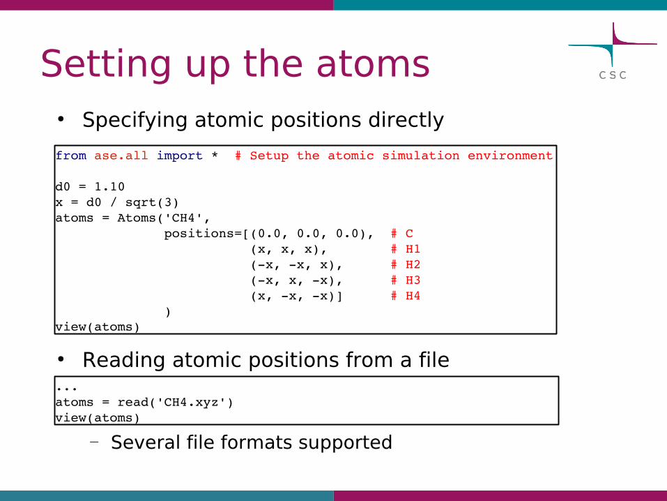
Setting up the atoms● Specifying atomic positions directly

from ase.all import *  # Setup the atomic simulation environment

d0 = 1.10x = d0 / sqrt(3)atoms = Atoms('CH4',               positions=[(0.0, 0.0, 0.0),  # C                         (x, x, x),        # H1                         (­x, ­x, x),      # H2                         (­x, x, ­x),      # H3                         (x, ­x, ­x)]      # H4              )view(atoms)

● Reading atomic positions from a file

― Several file formats supported

...atoms = read('CH4.xyz')view(atoms)

Setting up the unit cell● By default, the simulation cell of an Atoms object has

zero boundary conditions and edge length of 1 Å● Unit cell can be set when constructing Atoms

or later on

atoms = ...atoms.center(vacuum=3.5) # finite system 3.5 Å empty space around atoms

atoms = Atoms(...)   # positions in relative coordinatesatoms.set_cell((2.5, 2.5, 2.5), scale_atoms=True)atoms.set_pbc(True)  # or atoms.set_pbc((True, True, True))

atoms = Atoms(..., # positions must be now in absolute coordinates              cell=(1., 2., 3.), pbc=True)# or pbc=(True, True, True)

atoms = ...atoms.set_pbc((False, True, True)) # surface slabatoms.center(axis=0, vacuum=3.5) # 3.5 Å empty space in x­direction

Units in ASE● Length: Å● Energy: eV

● Easy conversion between units:

― also Rydberg, kcal, nm, ...

from ase.units import Bohr, Hartree

a = a0 * Bohr       # a0 in a.u., a in ÅE = E0 * Hartree    # E0 in Hartree, E in eV

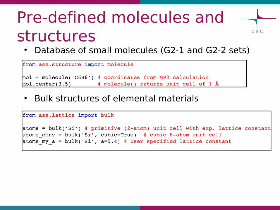
Pre-defined molecules and structures

● Database of small molecules (G2-1 and G2-2 sets)

from ase.structure import molecule

mol = molecule('C6H6') # coordinates from MP2 calculation mol.center(3.5)        # molecule() returns unit cell of 1 Å

● Bulk structures of elemental materials

from ase.lattice import bulk

atoms = bulk('Si') # primitive (2­atom) unit cell with exp. lattice constantatoms_conv = bulk('Si', cubic=True)  # cubic 8­atom unit cellatoms_my_a = bulk('Si', a=5.4) # User specified lattice constant

Supercells and surfaces● Existing Atoms objects can be “repeated” and

individual atoms removed

from ase.lattice import bulk

atoms = bulk('Si', cubic=True)  # cubic 8­atom unit cellsupercell = atoms.repeat((4, 4, 4)) # 512 atom supercelldel supercell[0]  # remove first atom, e.g. create a vacancy

● Utilities for working with surfacesfrom ase.lattice.surface import fcc111, add_adsorbate

slab = fcc111('Cu', size=(3,3,5)) # 5­layers of 3x3 Cu (111) surface# add O atom 2.5 Å above the surface in the 'bridge' siteadd_adsorbate(slab, 'O', 2.5, position='bridge')

Performing a calculation● In order to do calculation, one has to define a

calculator object and attach that to Atoms

● Specifying calculator parameters

● See wiki.fysik.dtu.dk/gpaw/documentation/manual.html for all parameters

from ase.structure import molecule   # Setup the atomic simulation environmentfrom gpaw import GPAW  # Setup GPAW

atoms = molecule('CH4')atoms.center(3.5)calc = GPAW() # Use default parametersatoms.set_calculator(calc)atoms.get_potential_energy() # Calculate the total energy

...calc = GPAW(h=0.18, nbands=6,        # 6 bands and grid spacing of 0.20 Å            kpts=(4,4,4),            # 4x4x4 Monkhorst­Pack k­mesh            xc='PBE', txt='out.txt') # PBE and print text output to file...

Performing a calculation

● Serial calculations and analysis can be carried out with normal Python interpreter

● Parallel calculations with gpaw-python executable

[jenkovaa@flamingo ~]$ python input.py

#!/bin/bash#SBATCH ­J gpaw_test#SBATCH ­t 00:30:00#SBATCH ­p parallel#SBATCH ­n 16

Module load gpaw­env/0.10.0

srun gpaw­python input.py

Structural optimization

● See wiki.fysik.dtu.dk/ase/ase/optimize.html for supported optimizers

● “Best” optimizer is case-dependent

from ase.all import *      # Setup the atomic simulation environmentfrom gpaw import GPAW      # Setup GPAW

atoms = ...calc = GPAW(...)atoms.set_calculator(calc)

opt = BFGS(atoms, trajectory='file.traj') # define an optimizeropt.run(fmax=0.05) # optimize the structure until forces smaller than 0.05 eV / Å 

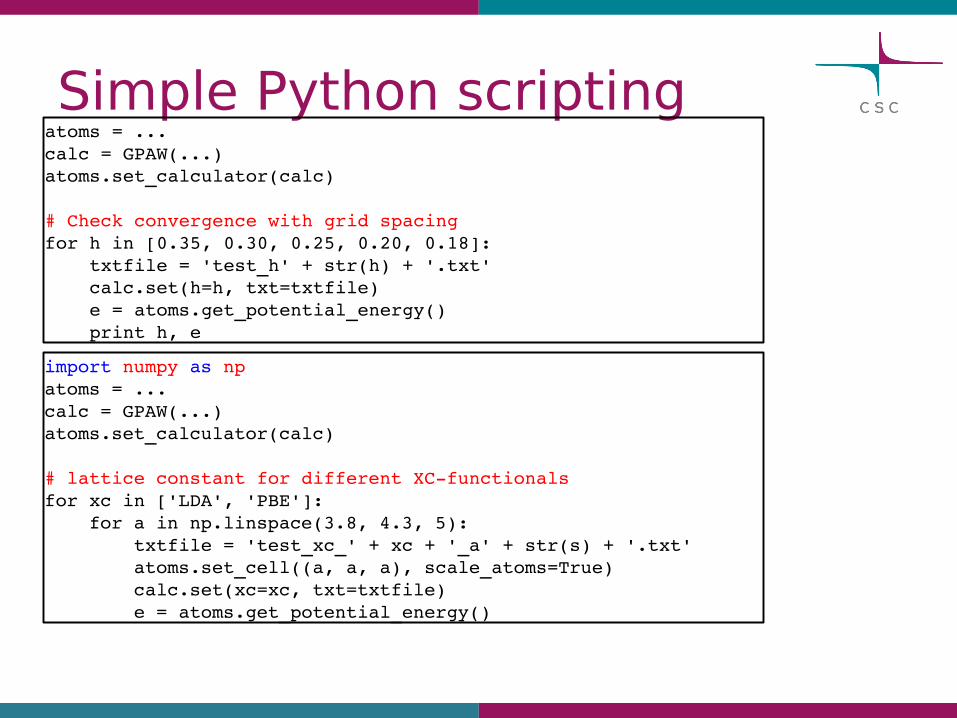
Simple Python scriptingatoms = ...calc = GPAW(...)atoms.set_calculator(calc)

# Check convergence with grid spacingfor h in [0.35, 0.30, 0.25, 0.20, 0.18]:    txtfile = 'test_h' + str(h) + '.txt'    calc.set(h=h, txt=txtfile)    e = atoms.get_potential_energy()    print h, e

import numpy as npatoms = ...calc = GPAW(...)atoms.set_calculator(calc)

# lattice constant for different XC­functionalsfor xc in ['LDA', 'PBE']:    for a in np.linspace(3.8, 4.3, 5):        txtfile = 'test_xc_' + xc + '_a' + str(s) + '.txt'        atoms.set_cell((a, a, a), scale_atoms=True)        calc.set(xc=xc, txt=txtfile)        e = atoms.get_potential_energy()

Saving and restarting● Saving full state of calculation: .gpw-files (or

.hdf5-files)

● Restarting

...calc = GPAW(...) atoms.set_calculator(calc)atoms.get_potential_energy() # Calculate the total energycalc.write('myfile.gpw')     # Atomic positions, densities, calculator parameters

...

calc.write('myfile.gpw', mode='all') # Save also wave functions (larger files)

...

calc.write('myfile.hdf5', mode='all') # If GPAW is build with HDF5 support

from ase.all import *   # Setup the atomic simulation environmentfrom gpaw import restart  # Setup GPAW

atoms, calc = restart('file.gpw')e0 = atoms.get_potential_energy() # no calculation neededcalc.set(h=0.20)e1 = atoms.get_potential_energy() # calculation total energy with new grid

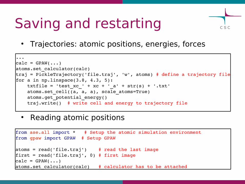
Saving and restarting● Trajectories: atomic positions, energies, forces

...calc = GPAW(...) atoms.set_calculator(calc)traj = PickleTrajectory('file.traj', 'w', atoms) # define a trajectory filefor a in np.linspace(3.8, 4.3, 5):    txtfile = 'test_xc_' + xc + '_a' + str(s) + '.txt'    atoms.set_cell((a, a, a), scale_atoms=True)    atoms.get_potential_energy()    traj.write()  # write cell and energy to trajectory file

● Reading atomic positions

from ase.all import *   # Setup the atomic simulation environmentfrom gpaw import GPAW  # Setup GPAW

atoms = read('file.traj')    # read the last image first = read('file.traj', 0) # first imagecalc = GPAW(...)atoms.set_calculator(calc)   # calculator has to be attached

Simple graphical interface (ase-gui)

● Trajectory can be investigated with ase-gui tool

[jenkovaa@flamingo ~]$ ase­gui file.traj

● Investigate how total energy, forces, bond lengths etc. vary during simulation