numerical heat and mass transfer - - università degli … degree in mechanical engineering fausto...

Master degree in Mechanical Engineering

Fausto Arpino [email protected]

Numerical Heat and Mass Transfer

06-Finite-Difference Method (One-dimensional, steady state heat conduction)

Introduction – Why we use models and how Many physical systems of interest are extremely complex, with many interacting elements governing their behavior. The way the complete system behaves may be explored by experiments. However, if it is a nonlinear system the effect of two changes made together is very different from the sum of the changes made separately so that it may be impossible to derive enough information from empirical parameter analysis. Alternatively, building or running experiments may be expensive or dangerous. Numerical models incorporate the knowledge gained by experiments allowing the running of new tests by computer simulations.

2

Physics approximation ü  Is the mathematical model available and able to accurately describe the physics of the system under

investigation? ü  In building computational models the skill required is to simulate as well as possible a physical system in

order to investigate its behavior. ü  The term as well as possible is subject to a whole range of conditions (on one hand the physics of the system

might be quite well known but the system may be so large that it is not possible to simulate it perfectly; on the other hand, the physics of the system is not so well known and we known just general behavior).

Numerical approximation ü  Pre-processing: consists of the input of a problem to CFD program by means of an user-friendly interface

and the subsequent transformation of the input into a form suitable for the solver. ü  Processing: consists of the numerical resolution of governing Partial Differential Equations (finite

difference, finite element, finite volume, spectral methods, etc. ü  Post-processing: consists of the results analysis (verification, validation,…)

3

Introduction – Main steps of numerical simulation

Mathematical model The quantities of interest are described by Partial Differential Equations (PDEs) in the form: Similar PDEs can be used for the resolution of different problems. The governing PDEs equations represent the mathematical statements of the conservation law of physics. EQUATIONS EXAMPLES...

ü  Transport equation

ü  Heat equation

ü  Waves equation 4

L ϕ,g( ) ≡ F x,θ,ϕ,∂ϕ

∂θ,∂ϕ∂x

,....,∂2ϕ

∂x 2,....,g

⎛

⎝⎜⎜⎜⎜

⎞

⎠⎟⎟⎟⎟

= 0

x

y

z

qx.

qy.

qx+dx.

qz.

qy+dy.

qz+dz.

ρc Tθ

u.Ω

Ω

∂ϕ∂θ

+∇ ⋅ uϕ( ) = 0

∂ϕ∂θ−∇2ϕ = G

∂2ϕ

∂θ2+∇2ϕ = 0

Since the exact solution φ(x,y,z,ϑ) can be very difficult to obtain, thought numerical models it is possible to obtain an approximated solution φN(xi,yi,zi,ϑi), with i=1,…,N, with the use of a computer

Exact operator

Approximated operator

A numerical method is convergent if: A numerical method is consistent if: A numerical method is stable small roundoff errors cause small (and convergent) solution oscillations.

Numerical modeling

5

L(ϕ,g) = 0

LN (ϕN ,gN ) = 0

ϕ(x,ϑ)

ϕi i = 1,...N

Numerical methods

lim

N→∞ϕ −ϕN = 0

lim

N→∞LN ϕ,g( ) = 0

LN ϕ,g( ) = L ϕ,g( ) + ETRoundoff error

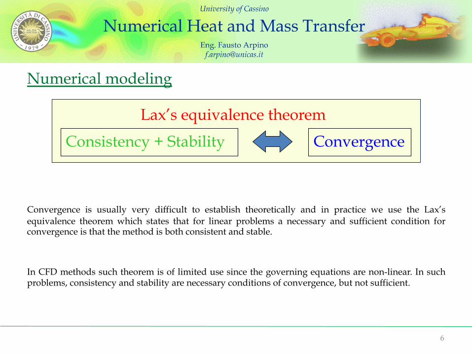
Convergence is usually very difficult to establish theoretically and in practice we use the Lax’s equivalence theorem which states that for linear problems a necessary and sufficient condition for convergence is that the method is both consistent and stable. In CFD methods such theorem is of limited use since the governing equations are non-linear. In such problems, consistency and stability are necessary conditions of convergence, but not sufficient.

6

Consistency + Stability Convergence

Lax’s equivalence theorem

Numerical modeling

The objective is then the construction of an equivalent, approximated operator, usually as a system of linear algebraic equations : How is it possible to achieve this goal? Finite difference: Finite-difference methods approximate the solutions to differential equations by approximating the derivative expressions in the governing equation; the method is easy to understand, but difficult to implement. Finite element: Based on the weak formulation and on the interpolation, the finite element method is less intuitive, but powerful, suitable for multiphysics and simple to implement. Finite volume: The Finite Volume method is a refined version of the finite difference method and has became popular in CFD.

7

∂...∂θ

+∇ ⋅.. +∇2.. = 0

a11ϕ1 + a12ϕ2.... + a1nϕn = 0

an1ϕ1 + an2ϕ2.... + annϕn = 0

⎧

⎨

⎪⎪⎪⎪

⎩⎪⎪⎪⎪

Numerical modeling

Finite-difference method for solving heat conduction problems The numerical method of solution is used in practical applications to determine the temperature distribution and heat flow in solids having complicated geometries, boundary conditions, and temperature-dependent properties. A commonly used numerical scheme (especially in the past) is the finite-difference method. In this method, the partial differential equation of heat conduction is approximated by a set of algebraic equations for temperature at a number of nodal points over the region. Since the method transforms the analysis of heat conduction problem to the solution of a set of coupled algebraic equations, it is also important to manage the methods of solving simultaneous algebraic equations. When a heat conduction problem is solved exactly by an analytical method, the resulting solution satisfies the governing differential equation at every domain point. When the problem is solved by a numerical method, such as finite-difference, the differential equation is satisfied only in correspondence of discrete number of points, called nodes. The finite-difference method can be developed by replacing the partial derivatives in the heat conduction equation with their equivalent finite-difference forms or writing an energy balance for a differential volume element.

8

1D Finite-difference method: Mathematical formulation

Consider the following one-dimensional, steady state heat conduction equation without energy generation The computational domain is discretized in space using a uniform grid (or mesh). The nodal temperature Ti is defined in each node of the computational grid.

It is assumed that the temperature in the domain is continuous, derivable with continuous and limited derivative. This assumption is necessary to find the approximate expression of the temperatures derivatives, with the aid of a Taylor series expansion .

9

2

20

d T

dx=

x

T

L

i i+1i-1

Δx

M0

With reference to the above discretized domain, the temperature Ti+1 at the node i+1 can be expressed as a function of the temperature Ti at the node i by using a Taylor series expansion.

(1)

Neglecting the second order terms, it is possible to obtain an approximated expression for the derivative at the node i (forward approximation):

10

x

T

L

i i+1i-1

Δx

M0

( )2 2

31 2 2i i

i i

dT d T xT T x o xdx dx+

Δ ⎡ ⎤= + Δ + + Δ⎣ ⎦

CUT OFF ERROR ( )1i i

i

dT T T o xdx x

+ −= + ΔΔ


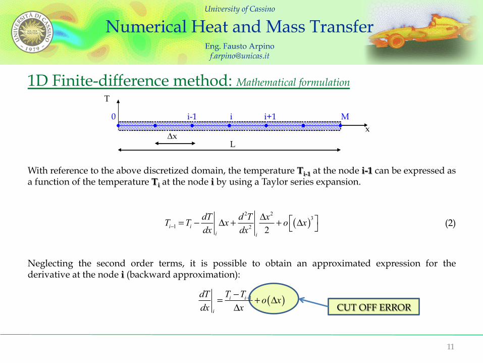
With reference to the above discretized domain, the temperature Ti-1 at the node i-1 can be expressed as a function of the temperature Ti at the node i by using a Taylor series expansion.

(2) Neglecting the second order terms, it is possible to obtain an approximated expression for the derivative at the node i (backward approximation):

11

x

T

L

i i+1i-1

Δx

M0

CUT OFF ERROR

( )2 2

31 2 2i i

i i

dT d T xT T x o xdx dx−

Δ ⎡ ⎤= − Δ + + Δ⎣ ⎦

( )1i i

i

dT T T o xdx x

−−= + ΔΔ


Both the derivative approximations (forward and backward) imply a leading error of order Δx. To reduce the cut off error it is necessary to reduce the elements dimension (Δx). It can be observed that subtracting eq. (2) from eq. (1) it is possible to obtain an expression of the temperature derivative with a second order approximation level (central approximation).

12

x

T

L

i i+1i-1

Δx

M0

1 1i iT T T+ −− = i T−2 2

222i

i i

dT d T xxdx dx

Δ+ Δ +2 2

2 2i

d T xdx

Δ− ( )3o x⎡ ⎤+ Δ⎣ ⎦

CUT OFF ERROR ( )21 1

2i i

i

dT T T o xdx x

+ −− ⎡ ⎤= + Δ⎣ ⎦Δ


13

x

T(x)

Ti

xi xi+1

Ti+1

Δx

α

( )1i i

i

dT T T o xdx x

+ −= + ΔΔ

( )2 2

31 2 2i i

i i

dT d T xT T x o xdx dx+

Δ ⎡ ⎤= + Δ + + Δ⎣ ⎦

i

dTdx

Graphic representation of the derivative forward approximation (first order)


14

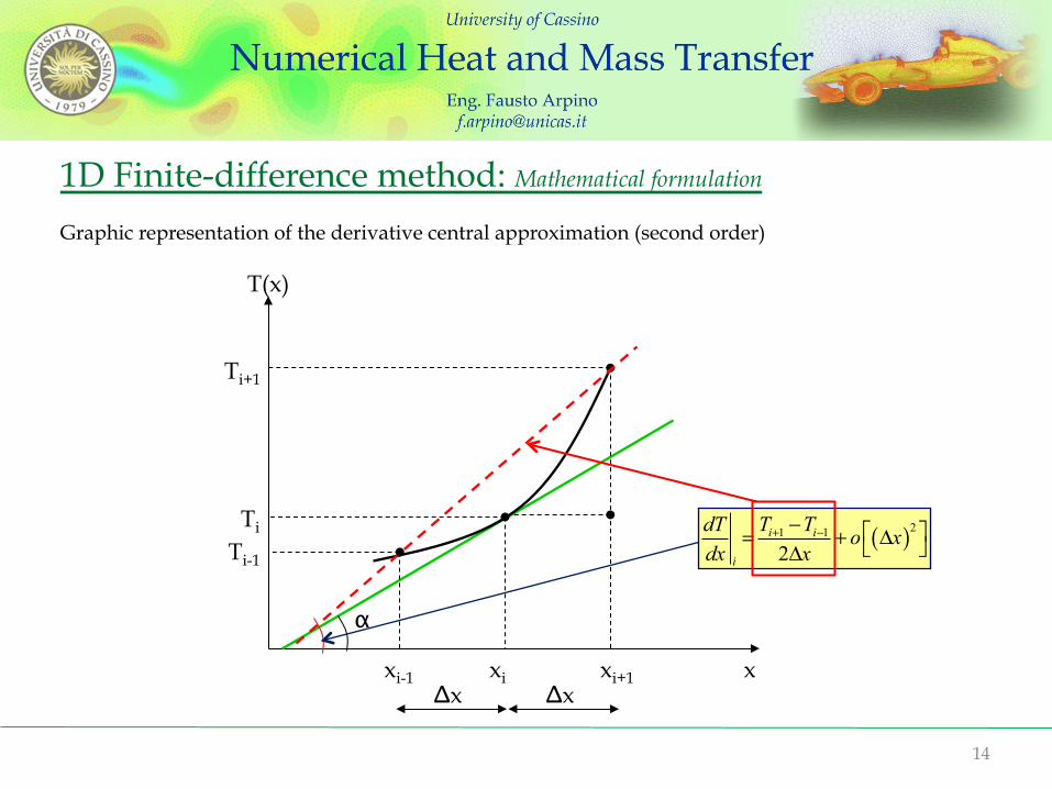
Graphic representation of the derivative central approximation (second order)

x

T(x)

Ti

xi xi+1

Ti+1

α

Ti-1

xi-1 Δx Δx

( )21 1

2i i

i

dT T T o xdx x

+ −− ⎡ ⎤= + Δ⎣ ⎦Δ


In a similar way, the second temperature derivative can be approximated by adding the members of the following equations: The final equation represents the approximated expression of the second derivative (central second derivative). In the case of internal nodes, the above analysis leads:

15

( )

( )

( )

2 2 3 34

1 2 3

2 2 3 34

1 2 3

231 1

2 2

2 6

2 6

2

i ii i i

i ii i i

i i i

i

dT d T x d T xT T x o xdx dx dx

dT d T x d T xT T x o xdx dx dx

d T T T T o xdx x

+

−

+ −

Δ Δ ⎡ ⎤= + Δ + + + Δ⎣ ⎦

+

Δ Δ ⎡ ⎤= − Δ + − + Δ⎣ ⎦

⇓

− + ⎡ ⎤= + Δ⎣ ⎦Δ

1 12 0i i iT T T+ −− + =


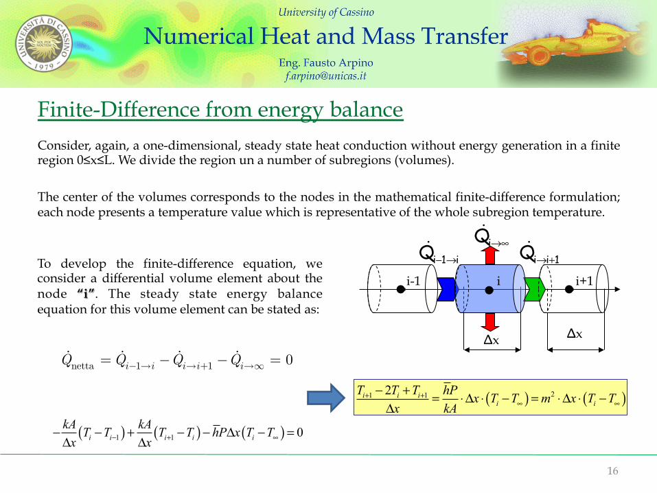
Finite-Difference from energy balance Consider, again, a one-dimensional, steady state heat conduction without energy generation in a finite region 0≤x≤L. We divide the region un a number of subregions (volumes). The center of the volumes corresponds to the nodes in the mathematical finite-difference formulation; each node presents a temperature value which is representative of the whole subregion temperature.

16

1iiQ +→!

Δx

i1iQ →−!

Δx

∞→iQ!

i-1 i+1 i

To develop the finite-difference equation, we consider a differential volume element about the node “i”. The steady state energy balance equation for this volume element can be stated as:

Qnetta = Qi−1→i −

Qi→i+1 −Qi→∞ = 0

( ) ( ) ( )1 1 0i i i i ikA kAT T T T hP x T Tx x− + ∞− − + − − Δ − =

Δ Δ

( ) ( )21 12i i ii i

T T T hP x T T m x T Tx kA

+ +∞ ∞

− + = ⋅ Δ ⋅ − = ⋅ Δ ⋅ −Δ

17

( ) ( )1 2M M MkA xT T hP T Tx − ∞

Δ− − = ⋅ ⋅ −Δ

Finite-Difference: Boundary Conditions The boundary conditions for heat conduction problem may be a prescribed temperature, prescribed heat flux or convection boundary condition.

Prescribed temperature The temperature T0 and TM at nodes x=0 and x=L are known and this provides the two additional relations needed to make the number of equations equal the number of unknown nodal temperatures

Prescribed heat flux (adiabatic end) Supposing that the heat flux is prescribed at the boundary x=L, to develop the finite-difference form of this boundary condition, we need to write the energy balance equation for a differential volume Dx/2 at node M.

x

Δx/2

M1MQ →−!

Δx

M-1 M

0Q =!

−

TM −TM−1

Δx= m2Δx

2TM −T∞( )

QM−1→M = QM→∞

Example: steady state heat conduction in a fin with adiabatic tip

18

Ts

L

(Adiabatic fin tip)

A

T∞ (surrounding fluid temperature)

h=hc+hi=cost

A=cross section area P=cross section perimeter

d2T

dx 2= m2 T −T∞( ) where m =

hPkA

⎛

⎝⎜⎜⎜⎞

⎠⎟⎟⎟⎟

( )0 sT T= 0L

dTdx

=

numerical heat and mass transfer - - università degli … degree in mechanical engineering fausto...

Documents