Numerical Integration and Rigid Body Dynamics for Potential

Field Planners

David Johnson

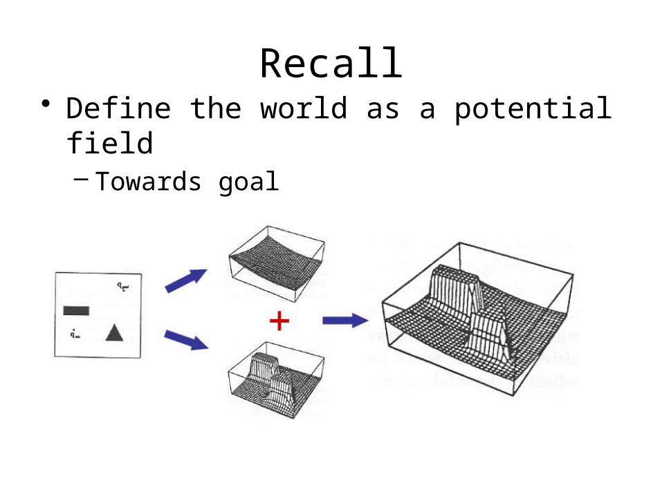
Recall• Define the world as a potential field

– Towards goal– Away from obstacles

Robot Motion• Move down the potential field to minimum

– Think about contours• Which way has zero change?• Which way has maximum?• The directional derivative gives the rate of change

in a direction: Duf(x,y) = f(x,y) . ∇ u

– Move along the gradient

),,()(1 nq

U

q

UqU

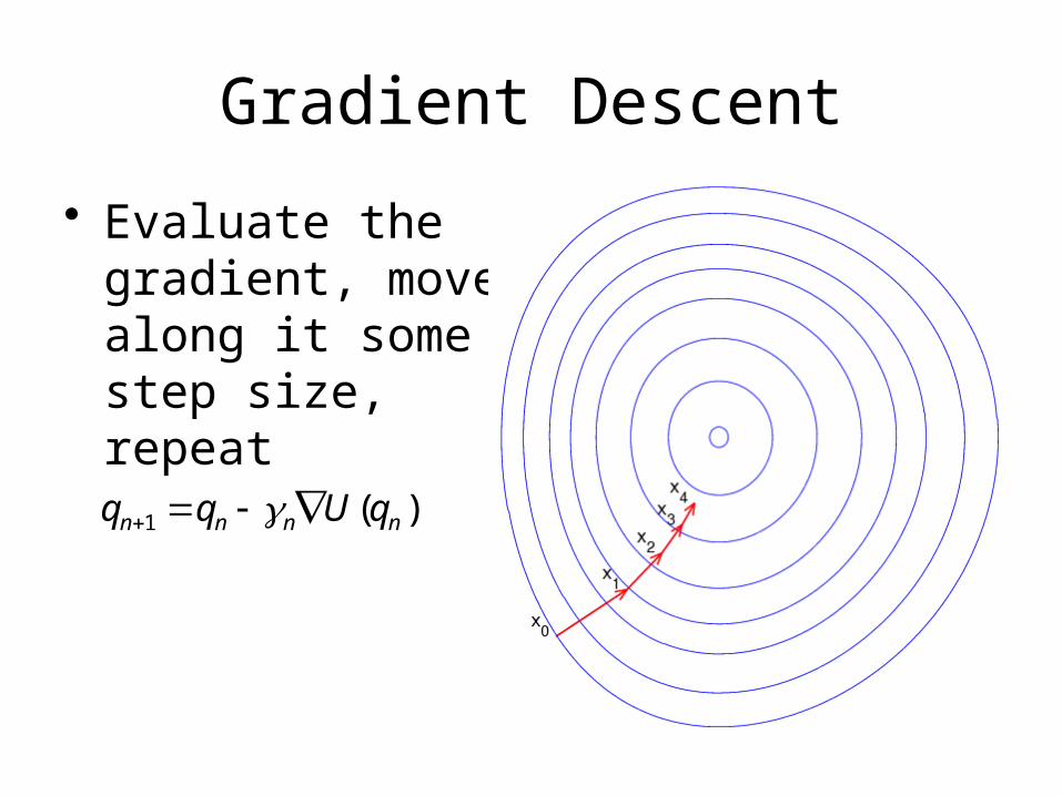
Gradient Descent

• Evaluate the gradient, move along it some step size, repeat

)(1 nnnn qUqq

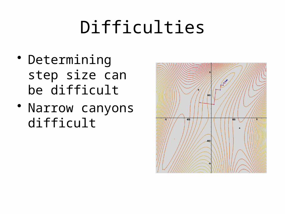
Difficulties

• Determining step size can be difficult

• Narrow canyons difficult

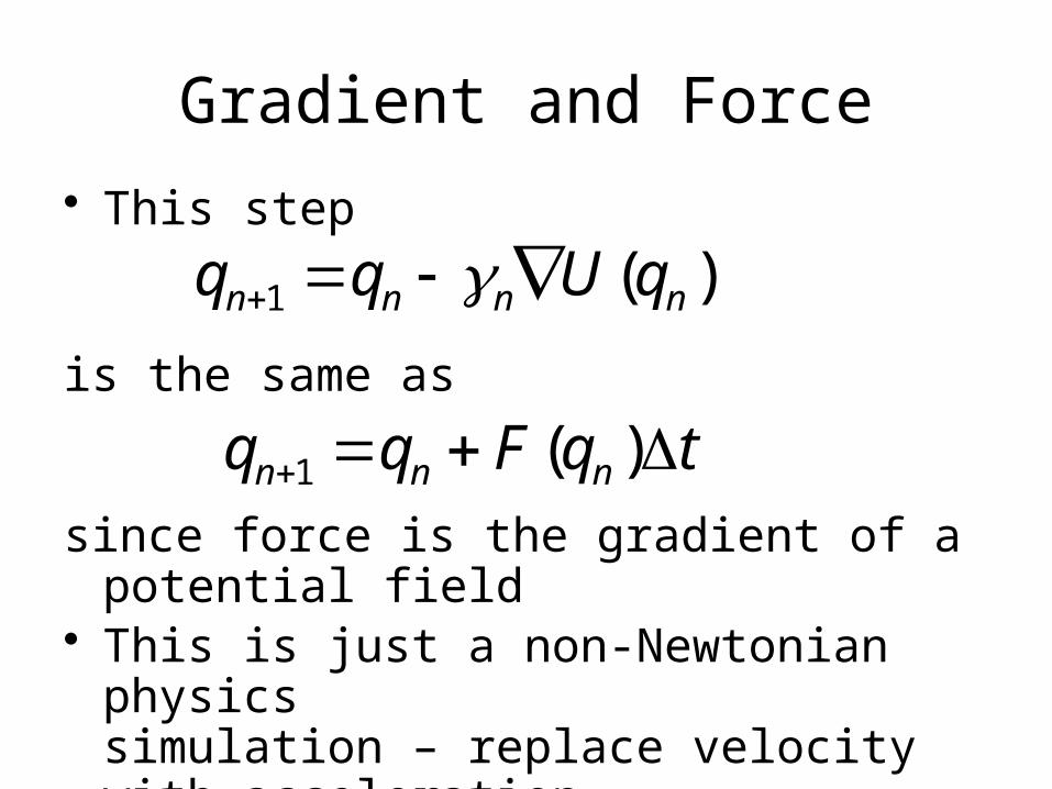
Gradient and Force

• This step

is the same as

since force is the gradient of a potential field• This is just a non-Newtonian physics

simulation – replace velocity with acceleration

)(1 nnnn qUqq

tqFqq nnn )(1

Potential Field vs Physics Simulation

• Potential field planner can thus also be seen as a physics simulation

• Robot has state (its configuration and velocities)

• Goal and obstacle apply forces• Evolve the state of the robot

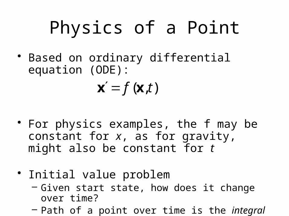
Physics of a Point

• Based on ordinary differential equation (ODE):

• For physics examples, the f may be constant for x, as for gravity, might also be constant for t

• Initial value problem– Given start state, how does it change over time?– Path of a point over time is the integral curve

),( tf xx

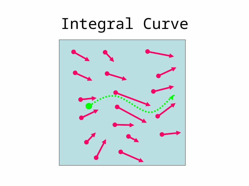
Integral Curve

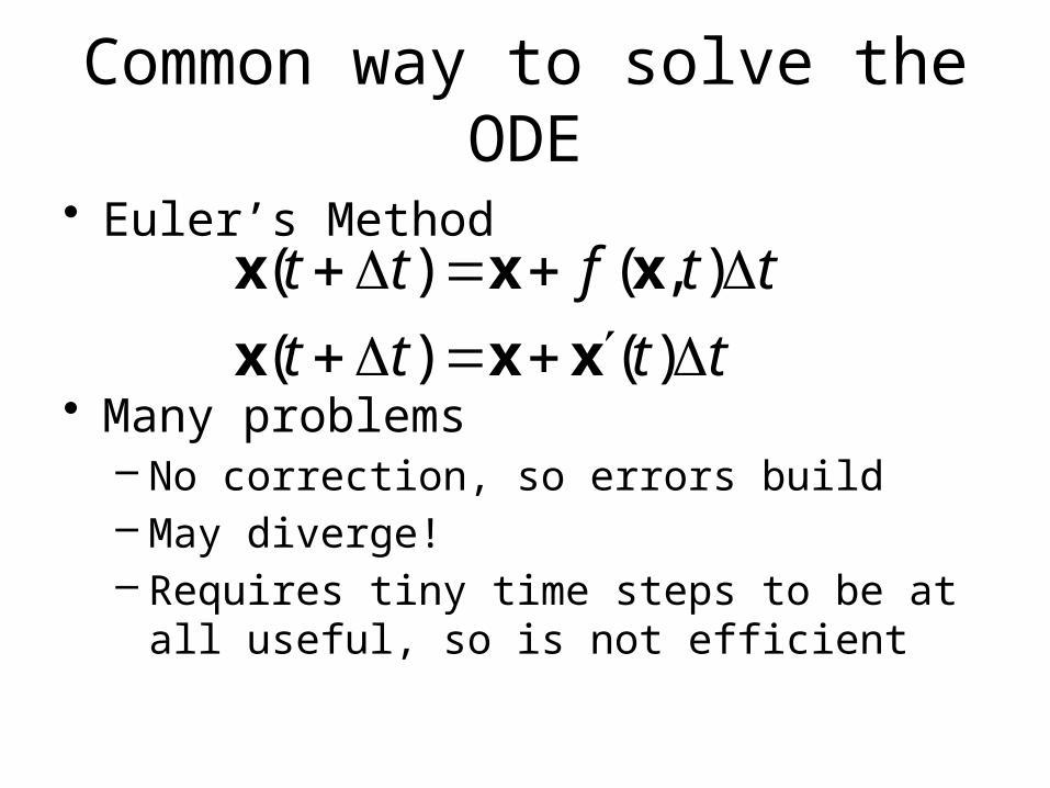
Common way to solve the ODE

• Euler’s Method

• Many problems– No correction, so errors build– May diverge!– Requires tiny time steps to be at all useful, so

is not efficient

tttt

ttftt

)()(

),()(

xxx

xxx

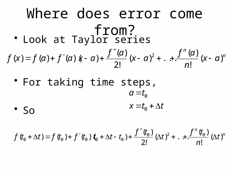
Where does error come from?• Look at Taylor series

• For taking time steps,

• So

nn

axn

afax

afaxafafxf )(

!

)(...)(

!2

)())(()()( 2

ttx

ta

0

0

nn

tn

tft

tfttttftfttf )(

!

)(...)(

!2

)())(()()( 02000000

Euler error

• Euler uses only first two terms of Taylor series

• Error dominated by missing quadratic

Use higher order

• Runge Kutta integration– Evaluates at multiple places to cancel out

error• Implicit integration

– Has to invert small matrix, but allows big steps

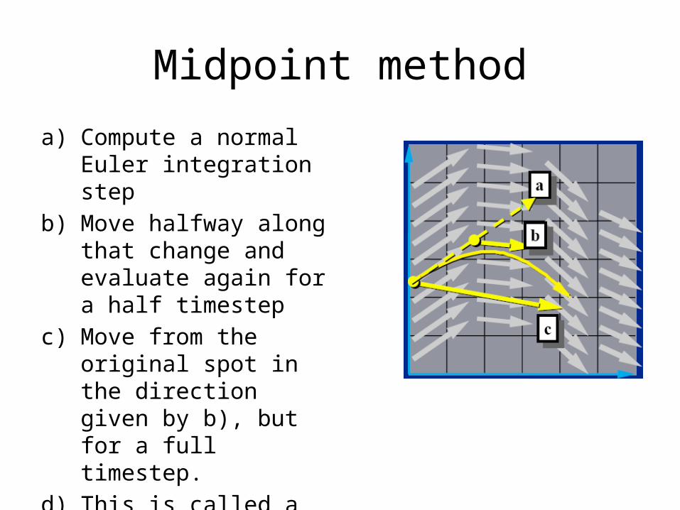
Midpoint method

a) Compute a normal Euler integration step

b) Move halfway along that change and evaluate again for a half timestep

c) Move from the original spot in the direction given by b), but for a full timestep.

d) This is called a second order method

Determine Stepsize

• Fixed– Simulation is only as fast as worst case

• Measure change in taking a step vs 2 half steps

Stiff ODEs• Equations with large constants

– Example: keep x at zero

– Euler integration

– Diverges if

kxx

t

ttt

xtk

tkxxx

)1(1

kt

tk

2

2

Stiff ODEs

• Can add energy into the system• Use friction to dampen the system

– Prevent out of control oscillations

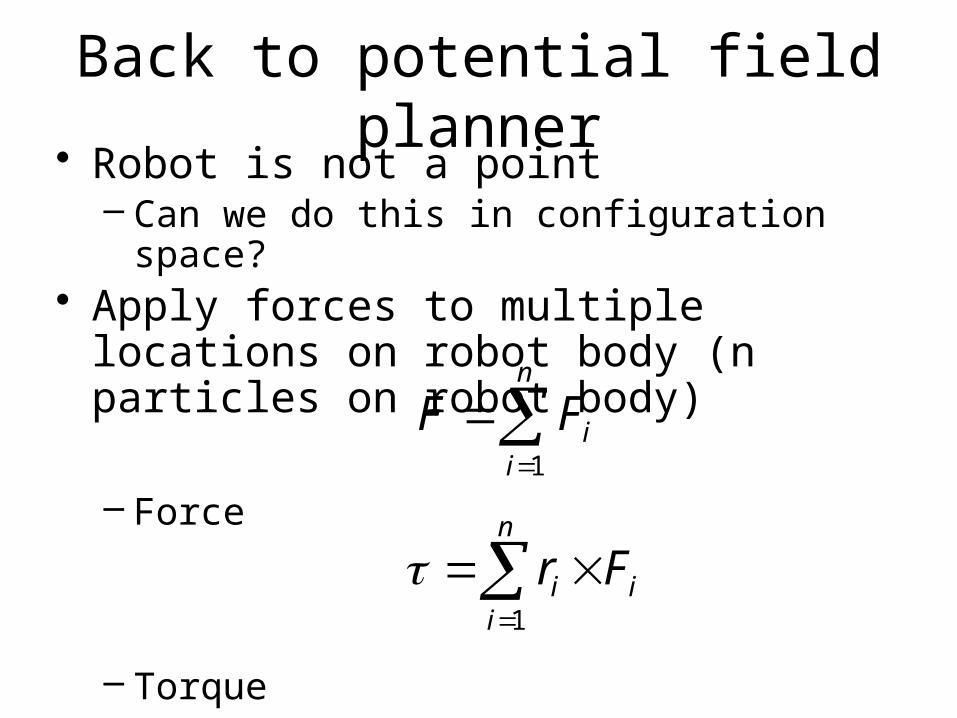
Back to potential field planner• Robot is not a point

– Can we do this in configuration space?• Apply forces to multiple locations on robot

body (n particles on robot body)

– Force

– Torque

n

iiFF

1

n

iii Fr

1

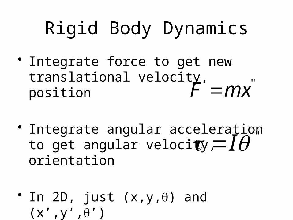
Rigid Body Dynamics

• Integrate force to get new translational velocity, position

• Integrate angular acceleration to get angular velocity, orientation

• In 2D, just (x,y,q) and (x’,y’,q’)• 3D is more complicated

'' I

''mxF

Back to Our Robot

• Sample points on the robot– Compute distance to goal– Compute distance to obstacles– Compute forces from each

• Apply forces to each point– Accumulate total force, total torque

• Do Euler integration to find new position, orientation