numerical investigation of stone columns system …...numerical investigation of stone columns...

Numerical investigation of stone columns system for liquefaction and settlement diminution potentialHaleh Meshkinghalam1, Masoud Hajialilue‑Bonab1* and Ali Khoshravan Azar2

BackgroundOne of the most important causes of failures or near failures of foundations, buildings and infrastructure facilities during earthquakes has been the development of liquefac-tion in saturated granular deposits. The technique of stone column as a method of soil improvement in situ is the most commonly adopted ground improvement technique for liquefaction over the last three decades. The fundamental concept of stone column is to replace susceptible soils to liquefaction with gravel in a vibratory manner, in order to reduce the liquefaction hazard and improve soil performance in four main ways. (1) Reducing the build-up of pore water pressure during and after earthquake by increasing drainage of the soil surrounding the columns. (2) Densification of the soil occurs around the stone column during installation, which improves the shear deformability of the soil skeleton to prevent large cyclic deformation during the earthquake. (3) Reinforcing the treated soil area since it is stiffer and stronger than the surrounding soil. (4) Increasing the lateral stresses in the soil surrounding the column.

Abstract

The aim of this study is the investigation of application of stone columns in decreasing liquefaction potential. Liquefaction potential of sand bed was studied by FLAC3D and validated by the results of VELACS international project. The effect of stone column was studied on decreasing excess pore pressure and soil settlement individually at the center of the model with different diameters. The effects of columns group were also studied on decreasing excess pore water pressure and soil settlement in a triangle arrangement. Finally an average vertical contact pressure of 100 kPa, which is approxi‑mately equal to the vertical pressure transmitted by a 10 story reinforced concrete building, was applied in the model. The implementation of stone columns individually, as a row or in groups with fewer numbers, caused a decrease in bulking in comparison to that of group using compressed meshing method. In certain numbers of columns, a decrease in distance among columns caused an increase in soil bulking. The columns group function will be better in settlement reduction, for center to center distance which is equal to 2.5–3.5 times of column’s diameter.

Keywords: Liquefaction, Soil improvement, Stone columns, FLAC3D

Open Access

© The Author(s) 2017. This article is distributed under the terms of the Creative Commons Attribution 4.0 International License (http://creativecommons.org/licenses/by/4.0/), which permits unrestricted use, distribution, and reproduction in any medium, provided you give appropriate credit to the original author(s) and the source, provide a link to the Creative Commons license, and indicate if changes were made.

ORIGINAL RESEARCH

Meshkinghalam et al. Geo-Engineering (2017) 8:11 DOI 10.1186/s40703-017-0047-x

*Correspondence: [email protected]; [email protected] 1 Department of Civil Engineering, University of Tabriz, Tabriz, IranFull list of author information is available at the end of the article

http://orcid.org/0000-0003-2865-2492

http://creativecommons.org/licenses/by/4.0/

http://crossmark.crossref.org/dialog/?doi=10.1186/s40703-017-0047-x&domain=pdf

of 24Meshkinghalam et al. Geo-Engineering (2017) 8:11

Different approaches have been proposed for the analysis of stone columns to miti-gate liquefaction under earthquake loading, ranging from simplified analytical proce-dure to physical modeling and to complex numerical analyses. The simplified procedure has introduced a design procedure, which takes into consideration pore pressure dis-sipation (drainage), as well as densification, for example Baez and Martin [1] and Shen-than [2]. The later method also takes into consideration the use of wick drains as part of the design procedure. These methods are popular because of their simplicity and the reduced number of required parameters, but they are unable to predict the soil move-ment and the pore pressure generation or dissipation. In addition, these methods have not been validated with field performance (Michael J. Quimby) [3]. These main short-comings of simplified analytical procedure can be overcome by using physical modeling and numerical techniques.

Significant research has been done for the physical modeling of stone column method using filed studies, shaking table and centrifuge test in the United States as well as in Japan. The main effects of stone column (drainage and stiffening) to mitigate liquefaction are investigated in varying soil condition by many researchers [4–9]. Although, these tests has provided valuable insight into stone column behavior to mitigate liquefaction during and after earthquake. Both shaking table and centrifuge model tests share cer-tain drawbacks, among the most important of which are similitude and boundary effects (Kramer). In addition they are time consuming and expensive. Due to these limitations of physical modeling, it is necessary to develop numerical technique to overcome them. The numerical technique so is investigated by many researchers [10–20].

Calculation of excess pore water pressure in the soil mass due to dynamic loading is the main factor in the modeling process of liquefaction phenomenon.

There are several different numerical approaches to model the behavior of a two-phase medium. Generally, they can be classified as uncoupled and coupled analyses. In the uncoupled analysis, the response of saturated soil is modelled without considering the effect of soil–water interaction, and then the pore water pressure is included separately by means of a pore pressure generation model. In the coupled analysis a formulation is used where all unknowns are computed simultaneously at each time step.

The numerical model is verified with centrifuge model test of verification of liquefac-tion analysis by centrifuge studies (VELACS). Results of this analysis proved that the finn model adopted in the FLAC computer code is able to model properly liquefaction.

Finn constitutive model for the soil in liquefaction simulationContrary to public perception, the pore water pressure during periodic loading is not directly related to periodic loading. The main effect of periodic loading is the creation of confining stresses in the space between soil grains, which decrease the space between soil grains. If the space between soil grains is filled with a fluid, then the fluid pressure will increase, leading to the decrease of effective stresses on soil grains. According to Eq. (1), this mechanism, which shows the relationship between the soil volume reduc-tion, Δεvd, and the size of periodic shear strains, γ, has been formulated by Martin et al. [21].

(1)�εvd = C1(γ − C2εvd)+C3ε

2vd

γ + C4εvd


where C1, C2, C3 and C4 are constants.Martin et al. [21] by assuming specified boundary conditions and certain coefficients,

Eq. (1) calculates the changes in fluid pressure through a porous medium. If the periodic shear strain equals zero, then the soil volume reduction will become zero, this implies that the constants are related as follows: C1C2C4 = C3. In 1991, Byrne presented Eq. (2), which is simpler than Martin’s formula where C1 and C2 are constants with different interpretations from those of Eq. (1). In most cases, C2 = 0.4

C1, so Eq. (2) will have one

unknown coefficient [21].

A constitutive model called Finn is formulated in FLAC3D, where Eqs. (1) and (2) are related to plastic Mohr–Coulomb model. Byrne stated that, according to the Eq. (3), the amount of C1 coefficient is dependent on sand relative density, Dr. Since Eq. (4) is estab-lished between soil relative density, Dr, and the normalized standard penetration test values, (N1)60, therefore according to Eq. (5), C1 coefficient will be related to the normal-ized standard penetration test values.

Further, using an empirical relation between Dr and normalized standard penetration test values, (N1)60:

Then,

C2 is then calculated from C2 = 0.4C1

in this case.Generally, in Finn model it is reasonable to measure the strain remnant. In Martin’s

studies, since the strain measurement is one dimensional, the strain remnant is speci-fied. However, in three dimensional analysis, there are at least 6 components of strain ratio tensor, which are calculated as shown below according to Eqs. (6–11) [21].

(2)�εvd

γ= C1exp

(

−C2

(

εvd

γ

))

(3)C1 = 7600D−2.5r

(4)Dr = 15(N1)−1.2560

(5)c1 = 8.7(N1)−1.2560

(6)ε1 = ε1 +�e12

(7)ε2 = ε2 +�e23

(8)ε3 = ε3 +�e31

(9)ε4 = ε4 +(�e11 −�e22)√

6

(10)ε5 = ε5 +(�e22 −�e33)√

6

(11)ε6 = ε6 +(�e33 −�e11)√

6


By calculating the engineering shear strain, γ, one can calculate the amount of soil vol-ume reduction, Δεvd, according to the Eq. (1) and as a result get the amount of εvd to use it in the Eq. (1) according to the Eq. (12).

FLAC3D also has the ability to calculate one third of the amount of �εvd in order to correct the amount of strain increase in next cycle according to Eqs. (13), (14) and (15):

It should be noted that in FLAC 3D, the increase of compressive strain has a negative sign and the amount of Δεvd is positive, so the effective stresses will decrease.

VerificationVELACS physical model

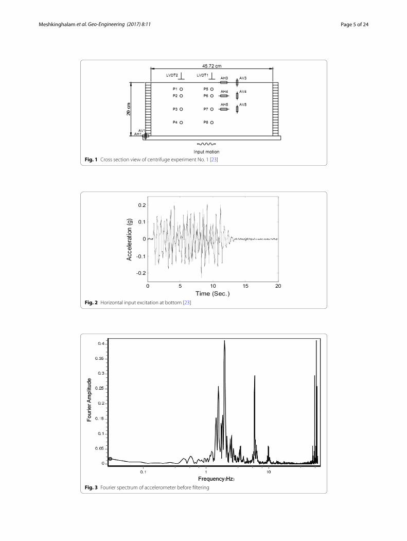
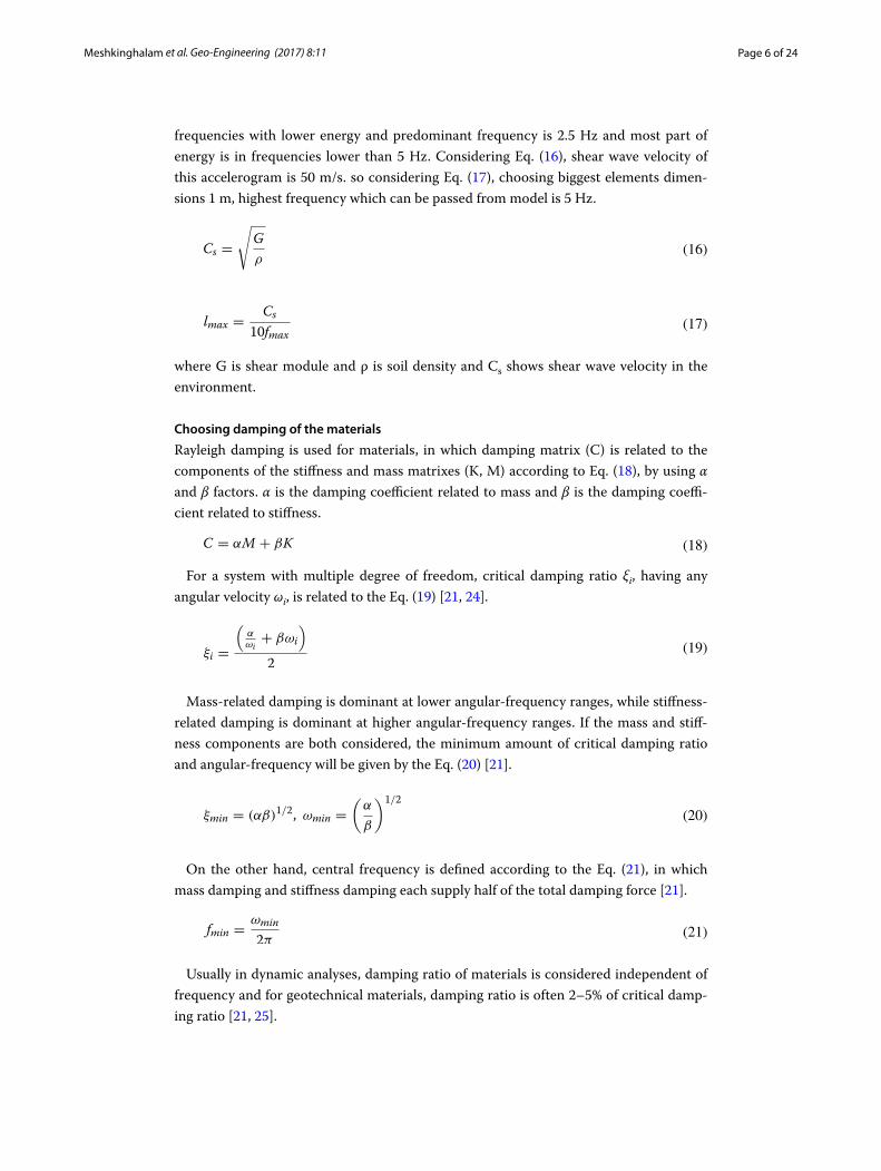
Test 1 of VELACS, CLASS B project was used for model validation. One layer of Nevada sand with uniform grading, 20 cm thickness and relative density of 40% in laminar box composed of 40 rectangular aluminum rings were used in this experiment. Characteris-tics of this Nevada sand have been shown in Table 1. By installation of rollers between rings, soil inside the box can move lateral directions to simulate behavior of sand in semi-finite environment during shakes. Sand layer has been saturated completely and it was rotated with 50g centrifuge acceleration. Model dimensions are as Fig. 1 and dynamic loading of the model was in the form of acceleration history in 20 cycles based on Fig. 2. Vertical acceleration was equal to zero [23].

Numerical simulation of VELACS physical model

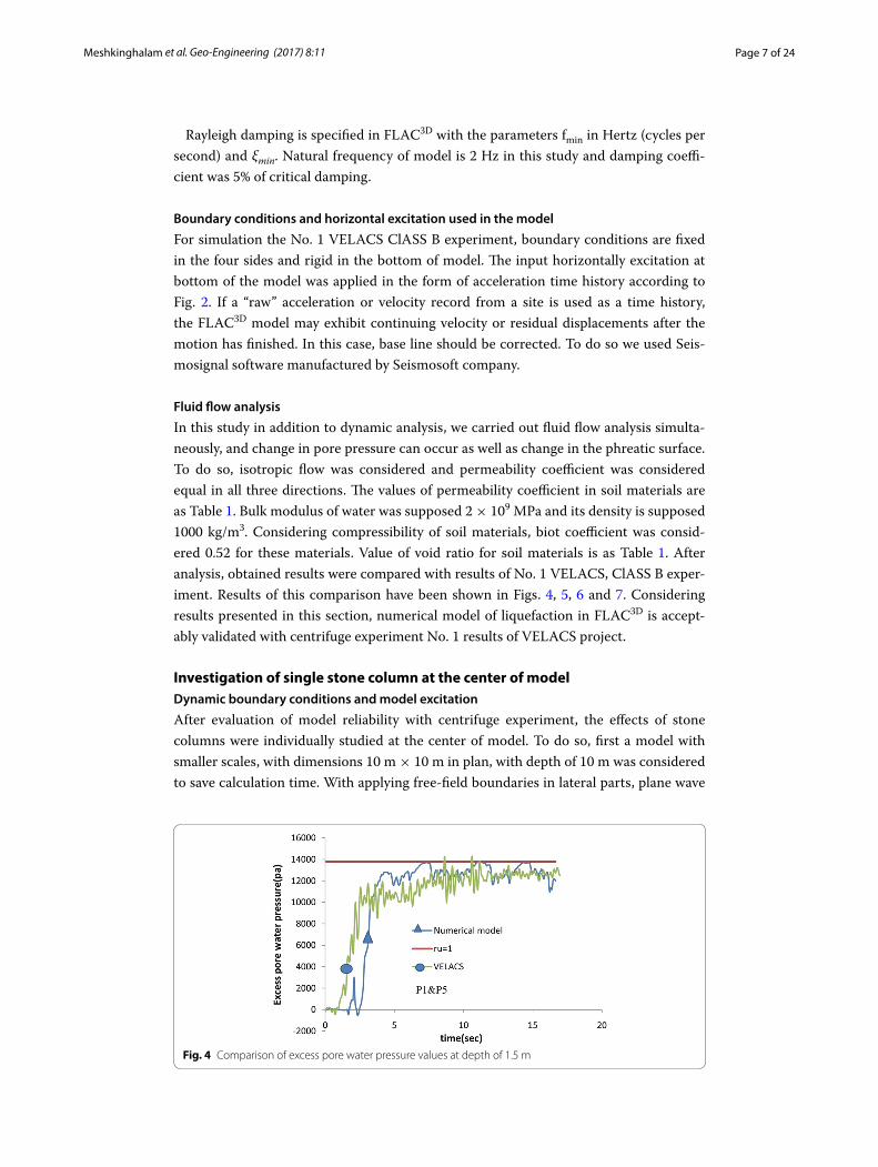
Considering dimensions and sizes of experiment No. 1 of VELACS project and the fact that, present test has scale coefficient of 1–50, geometry of numerical model in plan was selected as 23 × 10 m (23 m toward × direction and 10 m toward y direction) at depth of 10 m. Dynamic loading at lower part of model was in the form of acceleration history which can be seen in Fig. 2. Considering Fourier spectrum of accelerogram of centri-fuge experiment, Fig. 3, it can be seen that above mentioned accelerogram has higher

(12)εvd = εvd +�εvd

(13)�e11 = �e11 +�εvd

3

(14)�e22 = �e22 +�εvd

3

(15)�e33 = �e33 +�εvd

3

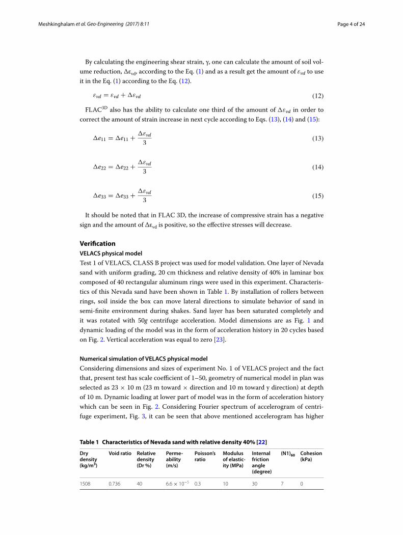
Table 1 Characteristics of Nevada sand with relative density 40% [22]

Dry density (kg/m3)

Void ratio Relative density (Dr %)

Perme-ability (m/s)

Poisson’s ratio

Modulus of elastic-ity (MPa)

Internal friction angle (degree)

(N1)60 Cohesion (kPa)

1508 0.736 40 6.6 × 10−5 0.3 10 30 7 0


Fig. 1 Cross section view of centrifuge experiment No. 1 [23]

Fig. 2 Horizontal input excitation at bottom [23]

Fig. 3 Fourier spectrum of accelerometer before filtering


frequencies with lower energy and predominant frequency is 2.5 Hz and most part of energy is in frequencies lower than 5 Hz. Considering Eq. (16), shear wave velocity of this accelerogram is 50 m/s. so considering Eq. (17), choosing biggest elements dimen-sions 1 m, highest frequency which can be passed from model is 5 Hz.

where G is shear module and ρ is soil density and Cs shows shear wave velocity in the environment.

Choosing damping of the materials

Rayleigh damping is used for materials, in which damping matrix (C) is related to the components of the stiffness and mass matrixes (K, M) according to Eq. (18), by using α and β factors. α is the damping coefficient related to mass and β is the damping coeffi-cient related to stiffness.

For a system with multiple degree of freedom, critical damping ratio ξi, having any angular velocity ωi, is related to the Eq. (19) [21, 24].

Mass-related damping is dominant at lower angular-frequency ranges, while stiffness-related damping is dominant at higher angular-frequency ranges. If the mass and stiff-ness components are both considered, the minimum amount of critical damping ratio and angular-frequency will be given by the Eq. (20) [21].

On the other hand, central frequency is defined according to the Eq. (21), in which mass damping and stiffness damping each supply half of the total damping force [21].

Usually in dynamic analyses, damping ratio of materials is considered independent of frequency and for geotechnical materials, damping ratio is often 2–5% of critical damp-ing ratio [21, 25].

(16)Cs =

√

G

ρ

(17)lmax =Cs

10fmax

(18)C = αM + βK

(19)ξi =

(

αωi

+ βωi

)

2

(20)ξmin = (αβ)1/2, ωmin =(

α

β

)1/2

(21)fmin =ωmin

2π


Rayleigh damping is specified in FLAC3D with the parameters fmin in Hertz (cycles per second) and ξmin. Natural frequency of model is 2 Hz in this study and damping coeffi-cient was 5% of critical damping.

Boundary conditions and horizontal excitation used in the model

For simulation the No. 1 VELACS ClASS B experiment, boundary conditions are fixed in the four sides and rigid in the bottom of model. The input horizontally excitation at bottom of the model was applied in the form of acceleration time history according to Fig. 2. If a “raw” acceleration or velocity record from a site is used as a time history, the FLAC3D model may exhibit continuing velocity or residual displacements after the motion has finished. In this case, base line should be corrected. To do so we used Seis-mosignal software manufactured by Seismosoft company.

Fluid flow analysis

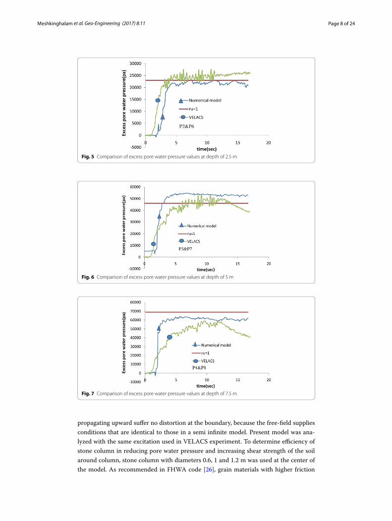
In this study in addition to dynamic analysis, we carried out fluid flow analysis simulta-neously, and change in pore pressure can occur as well as change in the phreatic surface. To do so, isotropic flow was considered and permeability coefficient was considered equal in all three directions. The values of permeability coefficient in soil materials are as Table 1. Bulk modulus of water was supposed 2 × 109 MPa and its density is supposed 1000 kg/m3. Considering compressibility of soil materials, biot coefficient was consid-ered 0.52 for these materials. Value of void ratio for soil materials is as Table 1. After analysis, obtained results were compared with results of No. 1 VELACS, ClASS B exper-iment. Results of this comparison have been shown in Figs. 4, 5, 6 and 7. Considering results presented in this section, numerical model of liquefaction in FLAC3D is accept-ably validated with centrifuge experiment No. 1 results of VELACS project.

Investigation of single stone column at the center of modelDynamic boundary conditions and model excitation

After evaluation of model reliability with centrifuge experiment, the effects of stone columns were individually studied at the center of model. To do so, first a model with smaller scales, with dimensions 10 m × 10 m in plan, with depth of 10 m was considered to save calculation time. With applying free-field boundaries in lateral parts, plane wave

Fig. 4 Comparison of excess pore water pressure values at depth of 1.5 m


propagating upward suffer no distortion at the boundary, because the free-field supplies conditions that are identical to those in a semi infinite model. Present model was ana-lyzed with the same excitation used in VELACS experiment. To determine efficiency of stone column in reducing pore water pressure and increasing shear strength of the soil around column, stone column with diameters 0.6, 1 and 1.2 m was used at the center of the model. As recommended in FHWA code [26], grain materials with higher friction


Fig. 6 Comparison of excess pore water pressure values at depth of 5 m



angle, lower cohesion and higher permeability are selected for stone columns. According to FHWA code, The Young modulus of stone columns materials should be 10–40 times more than surrounding soil. In this study is used coefficient of 40. Parameters used for stone column are as described in Table 2.

Interface elements between stone column materials and soil materials

Since soil and stone column materials are different, interface elements were used in con-tact area of column and soil. According to recommendation of FLAC3D software manual, a zone apparent stiffness in vertical direction can be calculated by Eq. (22).

where Kn and Ks are normal strength and shear strength for interface and K and G are bulk modulus and shear modulus of neighbor zones of interface, respectively, and ∆zmin is minimum width of zone in vertical direction. As it was mentioned earlier, since mate-rials of both sides of the interface are different from hardness aspect, due to recommen-dation of mentioned manual, this equation was used for softer and less rigid parts of the soil. So values of normal and shear strength of the interface is 135 MPa/m and cohesion and friction angle values of interface including surrounding soil of stone column are as Table 1. Using the same acceleration time history of VELACS experiment, recent model was also analyzed.

Permeable boundaries in fluid flow analysis

Upper boundaries of the model along with environmental boundaries of the stone col-umn, were defined as permeable boundaries in the software. It means that the flow can permeate from internal or external environment.

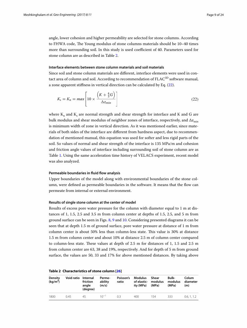
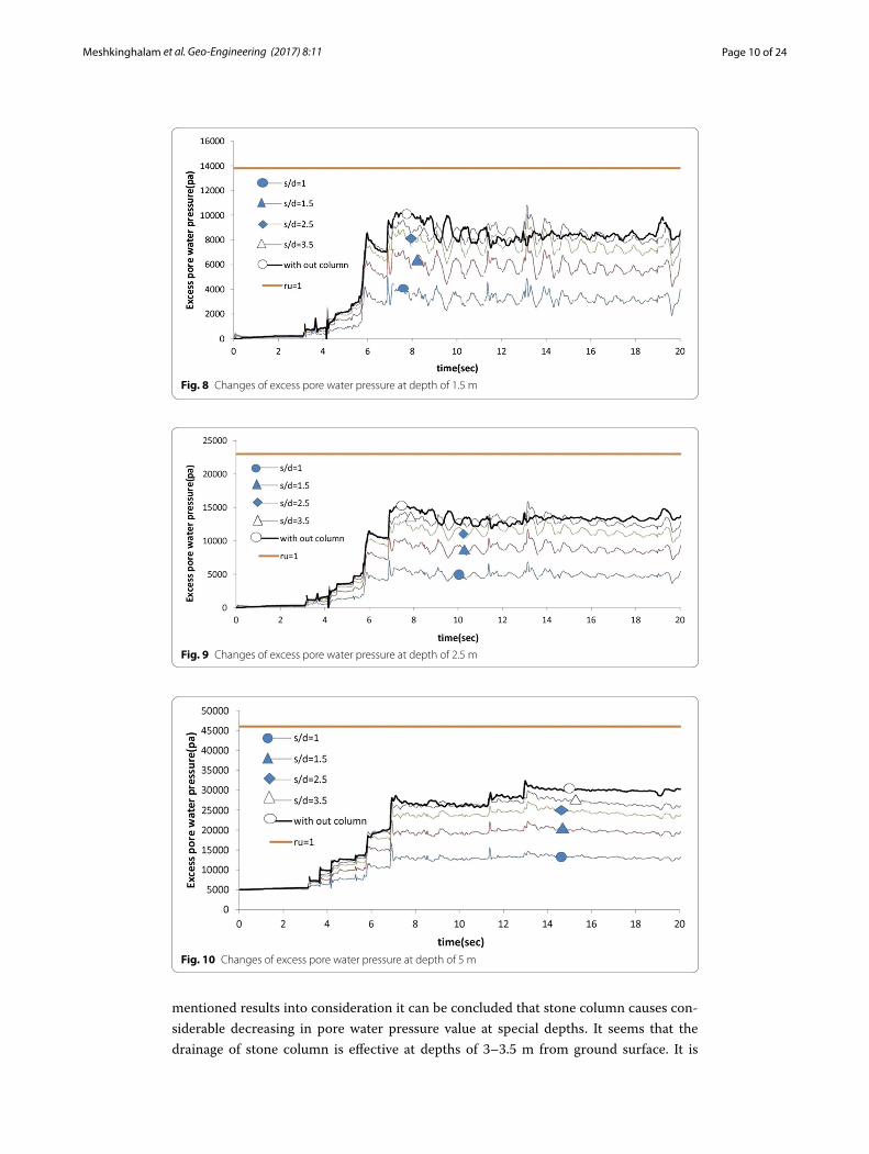
Results of single stone column at the center of model

Results of excess pore water pressure for the column with diameter equal to 1 m at dis-tances of 1, 1.5, 2.5 and 3.5 m from column center at depths of 1.5, 2.5, and 5 m from ground surface can be seen in Figs. 8, 9 and 10. Considering presented diagrams it can be seen that at depth 1.5 m of ground surface, pore water pressure at distance of 1 m from column center is about 50% less than column-less state. This value is 30% at distance 1.5 m from column center and about 10% at distance 2.5 m of column center compared to column-less state. These values at depth of 2.5 m for distances of 1, 1.5 and 2.5 m from column center are 63, 38 and 19%, respectively. And for depth of 5 m from ground surface, the values are 50, 33 and 17% for above mentioned distances. By taking above

(22)Ks = Kn = max

10×

�

K + 4

3G�

�zmin

Table 2 Characteristics of stone column [26]

Density (kg/m3)

Void ratio Internal friction angle (degree)

Perme-ability (m/s)

Poisson’s ratio

Modulus of elastic-ity (MPa)

Shear modulus (MPa)

Bulk-modulus (MPa)

Colum diameter (m)

1800 0.45 45 10−1 0.3 400 154 333 0.6, 1, 1.2


mentioned results into consideration it can be concluded that stone column causes con-siderable decreasing in pore water pressure value at special depths. It seems that the drainage of stone column is effective at depths of 3–3.5 m from ground surface. It is

Fig. 8 Changes of excess pore water pressure at depth of 1.5 m

Fig. 9 Changes of excess pore water pressure at depth of 2.5 m

Fig. 10 Changes of excess pore water pressure at depth of 5 m


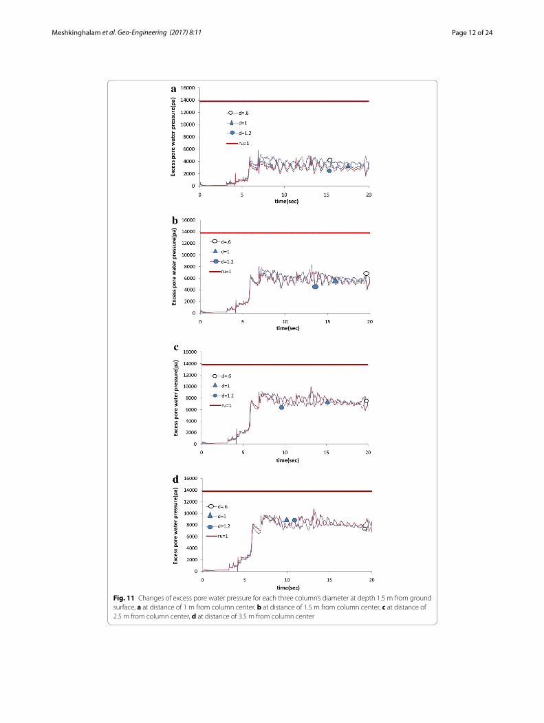
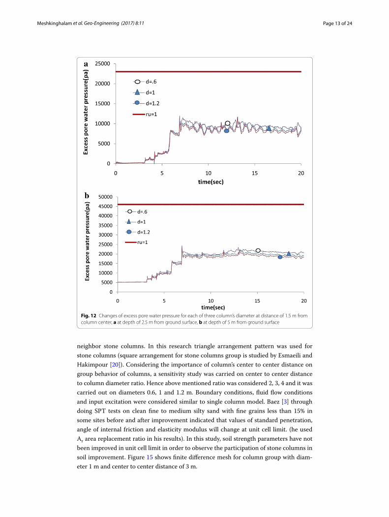
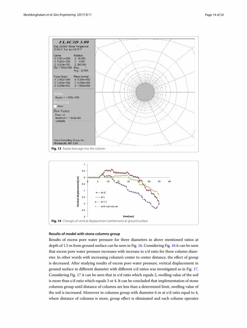
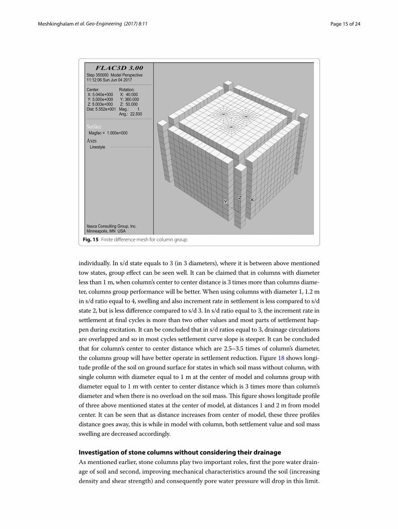
of course worth mentioning that in this research in depth lower than 5 m, liquefaction potential was lower due to increasing overload and at depths more than 5 m are vulner-able to liquefaction. It is also observed that with increasing in depth, pore water pressure fluctuation is decreased and pore water pressure reaches stability at more cycles. This is due to increasing load and increasing effective stress. Moreover it is observed that excess pore water pressure at distances of 1, 1.5 and 2.5 m from column center is decreased compared to column-less state. This is while in the distance of 3.5 m from column center, excess pore water pressure value is not significantly different from column-less state. So it can be concluded that stone column causes drainage at area in 2.5 m from its center. The effect of column drainage is vanished in distance more than 2.5 m. excess pore water pressure changes for columns with diameter 0.6 and 1.2 m occur like above mentioned diagrams. After studying effects of distance column center in pore water drainage, diam-eter of column was investigated in decreasing excess pore water pressure. Hence, first, changes of pore water pressure is compared for three diameters at distances of 1, 1.5, 2.5 and 3.5 m from column center at depth of 1.5 m from ground surface as in Fig. 11. Next in order to study effects of column diameter at different depths, diagrams of excess pore water pressure against time for three diameters is compared at distance of 1.5 m from column center and at depths of 2.5 and 5 m from ground surface with similar conditions at depth 1.5 m from ground surface as in Fig. 12. It can be seen that at all three depths till distance 1–1.5 m from column center, increase of column diameter results in increase of drainage, this is while at distance more than 1.5 m increase of column diameter has no effect on pore water drainage and all three diameters of the column show similar behav-ior. Considering Fig. 12 and comparing it with Fig. 11 it can be seen that with increase in depth, the effect of column diameter is decreased in pore water drainage. Moreover it was observed that deeper layers confront pore water pressure drops faster than super-ficial layers. Figure 13 shows water flow vectors inside stone column which indicates radial drainage of water flow in soil mass to inside the column. In this section vertical translocation without column state and with single stone column at the center were investigated. Vertical displacement changes in ground surface during dynamic loading are as shown in Fig. 14. It can be seen that at first, increment rate in settlement is less than compared to column-less state. Then it is increased at final cycles. This is while it can be seen at final cycles that gravel grains of stone columns are coarser than sur-rounding soil, having more void space, hence pore water pressure dissipated faster and more settlement happened at short time. It can be moreover observed that, in column-less state, slope of settlement curve at some cycle, specially at final cycles, is about zero, though it is not observed in model with stone column. The reason of this is that, more percent of settlement in model with column happen during excitation.

Investigation of model with stone columns group

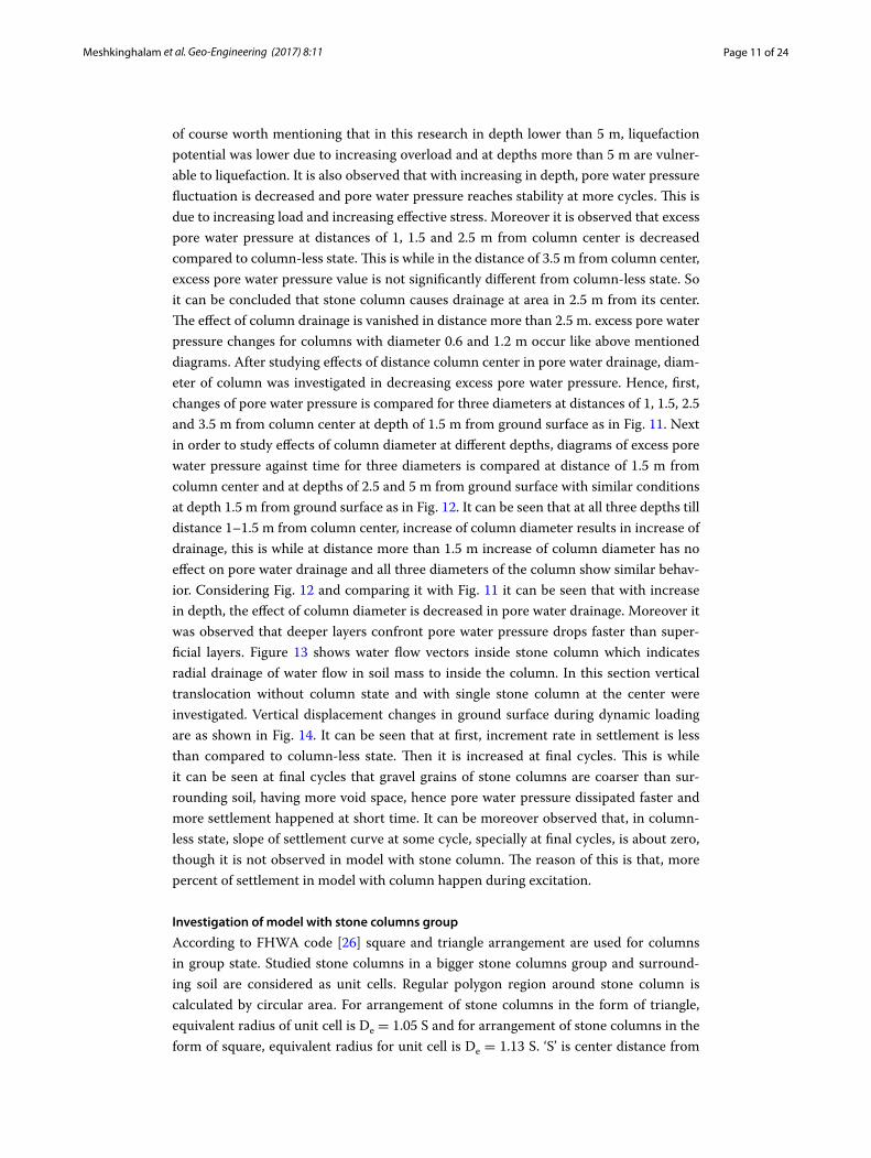
According to FHWA code [26] square and triangle arrangement are used for columns in group state. Studied stone columns in a bigger stone columns group and surround-ing soil are considered as unit cells. Regular polygon region around stone column is calculated by circular area. For arrangement of stone columns in the form of triangle, equivalent radius of unit cell is De = 1.05 S and for arrangement of stone columns in the form of square, equivalent radius for unit cell is De = 1.13 S. ‘S’ is center distance from


Fig. 11 Changes of excess pore water pressure for each three column’s diameter at depth 1.5 m from ground surface, a at distance of 1 m from column center, b at distance of 1.5 m from column center, c at distance of 2.5 m from column center, d at distance of 3.5 m from column center


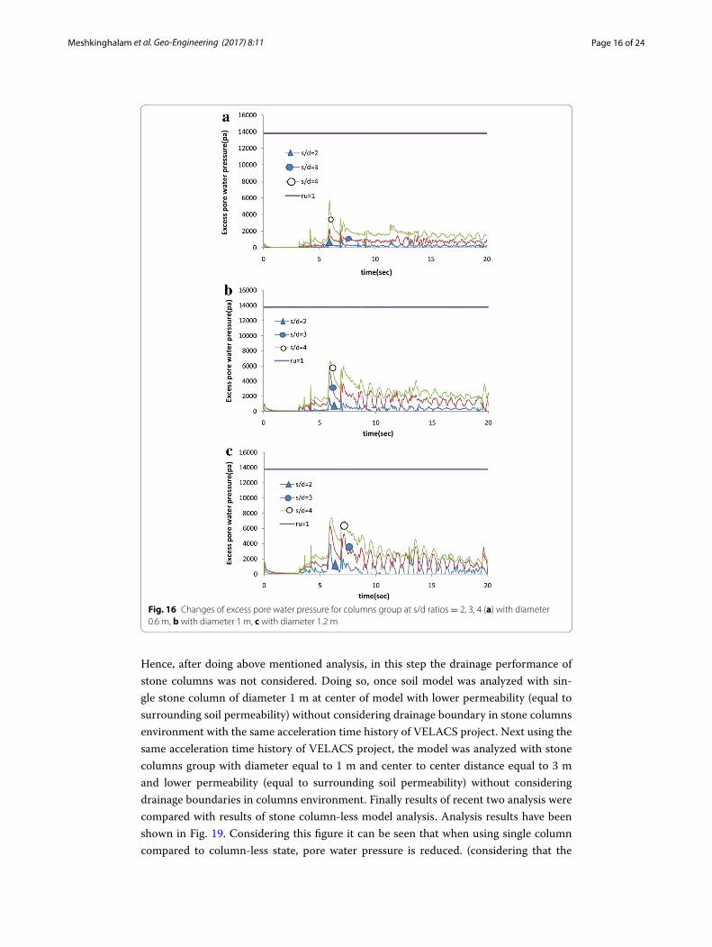
neighbor stone columns. In this research triangle arrangement pattern was used for stone columns (square arrangement for stone columns group is studied by Esmaeili and Hakimpour [20]). Considering the importance of column’s center to center distance on group behavior of columns, a sensitivity study was carried on center to center distance to column diameter ratio. Hence above mentioned ratio was considered 2, 3, 4 and it was carried out on diameters 0.6, 1 and 1.2 m. Boundary conditions, fluid flow conditions and input excitation were considered similar to single column model. Baez [3] through doing SPT tests on clean fine to medium silty sand with fine grains less than 15% in some sites before and after improvement indicated that values of standard penetration, angle of internal friction and elasticity modulus will change at unit cell limit. (he used Ar area replacement ratio in his results). In this study, soil strength parameters have not been improved in unit cell limit in order to observe the participation of stone columns in soil improvement. Figure 15 shows finite difference mesh for column group with diam-eter 1 m and center to center distance of 3 m.

Fig. 12 Changes of excess pore water pressure for each of three column’s diameter at distance of 1.5 m from column center, a at depth of 2.5 m from ground surface, b at depth of 5 m from ground surface


Results of model with stone columns group

Results of excess pore water pressure for three diameters in above mentioned ratios at depth of 1.5 m from ground surface can be seen in Fig. 16. Considering Fig. 16 it can be seen that excess pore water pressure increases with increase in s/d ratio for three column diam-eter. In other words with increasing column’s center to center distance, the effect of group is decreased. After studying results of excess pore water pressure, vertical displacement in ground surface in different diameter with different s/d ratios was investigated as in Fig. 17. Considering Fig. 17 it can be seen that in s/d ratio which equals 2, swelling value of the soil is more than s/d ratio which equals 3 or 4. It can be concluded that implementation of stone columns group until distance of columns are less than a determined limit, swelling value of the soil is increased. Moreover in columns group with diameter 6 m at s/d ratio equal to 4, where distance of columns is more, group effect is eliminated and each column operates

Fig. 13 Radial drainage into the column

Fig. 14 Changes of vertical displacement (settlement) at ground surface


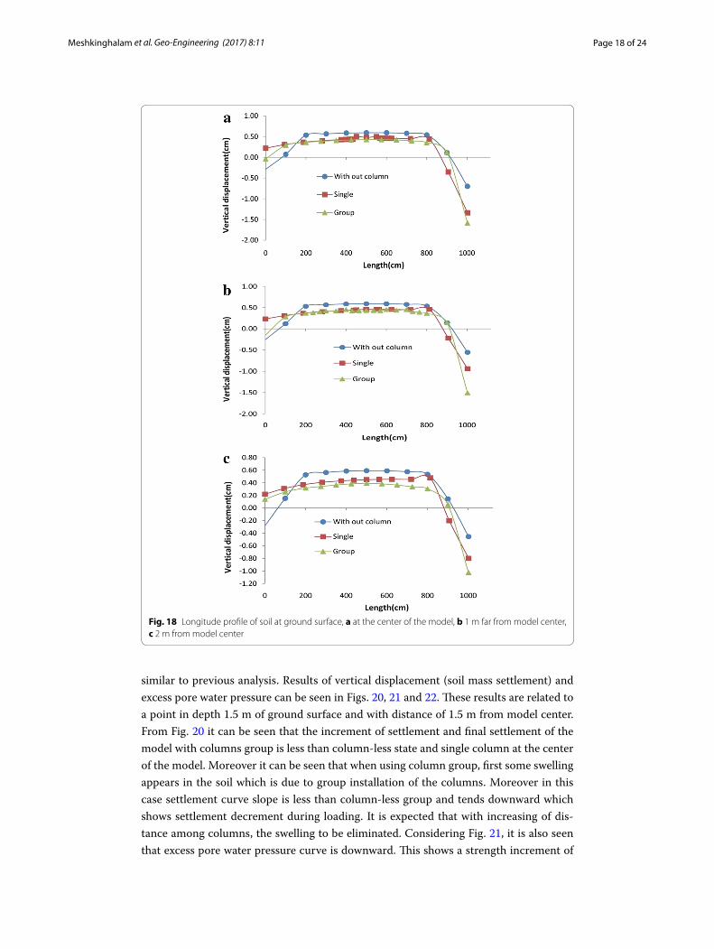
individually. In s/d state equals to 3 (in 3 diameters), where it is between above mentioned tow states, group effect can be seen well. It can be claimed that in columns with diameter less than 1 m, when column’s center to center distance is 3 times more than columns diame-ter, columns group performance will be better. When using columns with diameter 1, 1.2 m in s/d ratio equal to 4, swelling and also increment rate in settlement is less compared to s/d state 2, but is less difference compared to s/d 3. In s/d ratio equal to 3, the increment rate in settlement at final cycles is more than two other values and most parts of settlement hap-pen during excitation. It can be concluded that in s/d ratios equal to 3, drainage circulations are overlapped and so in most cycles settlement curve slope is steeper. It can be concluded that for column’s center to center distance which are 2.5–3.5 times of column’s diameter, the columns group will have better operate in settlement reduction. Figure 18 shows longi-tude profile of the soil on ground surface for states in which soil mass without column, with single column with diameter equal to 1 m at the center of model and columns group with diameter equal to 1 m with center to center distance which is 3 times more than column’s diameter and when there is no overload on the soil mass. This figure shows longitude profile of three above mentioned states at the center of model, at distances 1 and 2 m from model center. It can be seen that as distance increases from center of model, these three profiles distance goes away, this is while in model with column, both settlement value and soil mass swelling are decreased accordingly.

Investigation of stone columns without considering their drainageAs mentioned earlier, stone columns play two important roles, first the pore water drain-age of soil and second, improving mechanical characteristics around the soil (increasing density and shear strength) and consequently pore water pressure will drop in this limit.

Fig. 15 Finite difference mesh for column group


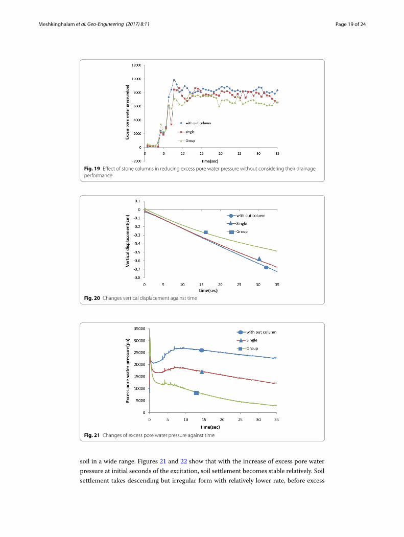
Hence, after doing above mentioned analysis, in this step the drainage performance of stone columns was not considered. Doing so, once soil model was analyzed with sin-gle stone column of diameter 1 m at center of model with lower permeability (equal to surrounding soil permeability) without considering drainage boundary in stone columns environment with the same acceleration time history of VELACS project. Next using the same acceleration time history of VELACS project, the model was analyzed with stone columns group with diameter equal to 1 m and center to center distance equal to 3 m and lower permeability (equal to surrounding soil permeability) without considering drainage boundaries in columns environment. Finally results of recent two analysis were compared with results of stone column-less model analysis. Analysis results have been shown in Fig. 19. Considering this figure it can be seen that when using single column compared to column-less state, pore water pressure is reduced. (considering that the

Fig. 16 Changes of excess pore water pressure for columns group at s/d ratios = 2, 3, 4 (a) with diameter 0.6 m, b with diameter 1 m, c with diameter 1.2 m


effect of stone column drainage has not been taken into consideration). When using col-umn group, increase and decrease process of pore water pressure indicate most changes compared to single column state. The reason for this is that columns group improve the mechanical characteristics of the soil in more limits compared to single column.

Investigation of model under the loadingIn this stage, an average vertical contact pressure of 100 kPa, which is approximately equal to the vertical pressure transmitted by a 10 story reinforced concrete building, was applied in the model. Hence stone column-less model, single stone column with diameter equal to 1 m in the center of the model and stone columns group with diam-eter equal to 1 m in a triangular arrangement with s/d ratio equal to 3 were used. Static and dynamic boundary conditions and acceleration time history were exactly similar to the models analyzed without overload. Moreover fluid flow analysis of this model was

Fig. 17 Changes of vertical displacement (settlement) at ground surface for columns group with s/d ratios of = 2, 3, 4 (a) diameter 0.6 m, b diameter 1 m, c with diameter 1.2 m


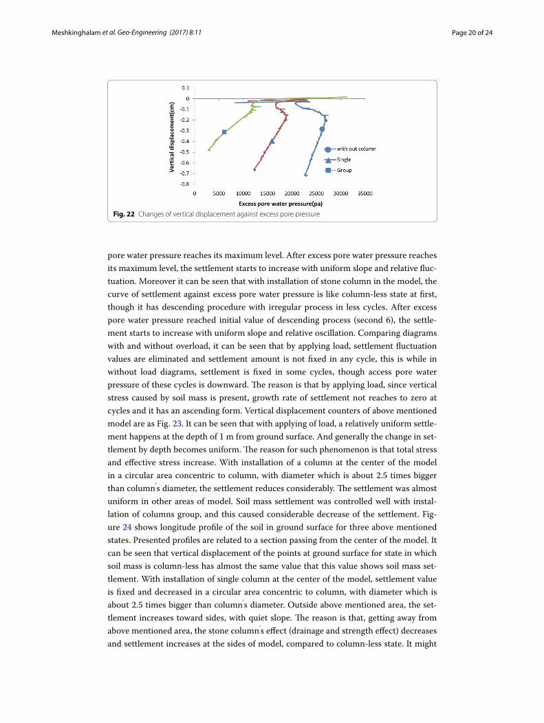
similar to previous analysis. Results of vertical displacement (soil mass settlement) and excess pore water pressure can be seen in Figs. 20, 21 and 22. These results are related to a point in depth 1.5 m of ground surface and with distance of 1.5 m from model center. From Fig. 20 it can be seen that the increment of settlement and final settlement of the model with columns group is less than column-less state and single column at the center of the model. Moreover it can be seen that when using column group, first some swelling appears in the soil which is due to group installation of the columns. Moreover in this case settlement curve slope is less than column-less group and tends downward which shows settlement decrement during loading. It is expected that with increasing of dis-tance among columns, the swelling to be eliminated. Considering Fig. 21, it is also seen that excess pore water pressure curve is downward. This shows a strength increment of

Fig. 18 Longitude profile of soil at ground surface, a at the center of the model, b 1 m far from model center, c 2 m from model center


soil in a wide range. Figures 21 and 22 show that with the increase of excess pore water pressure at initial seconds of the excitation, soil settlement becomes stable relatively. Soil settlement takes descending but irregular form with relatively lower rate, before excess

Fig. 19 Effect of stone columns in reducing excess pore water pressure without considering their drainage performance

Fig. 20 Changes vertical displacement against time

Fig. 21 Changes of excess pore water pressure against time


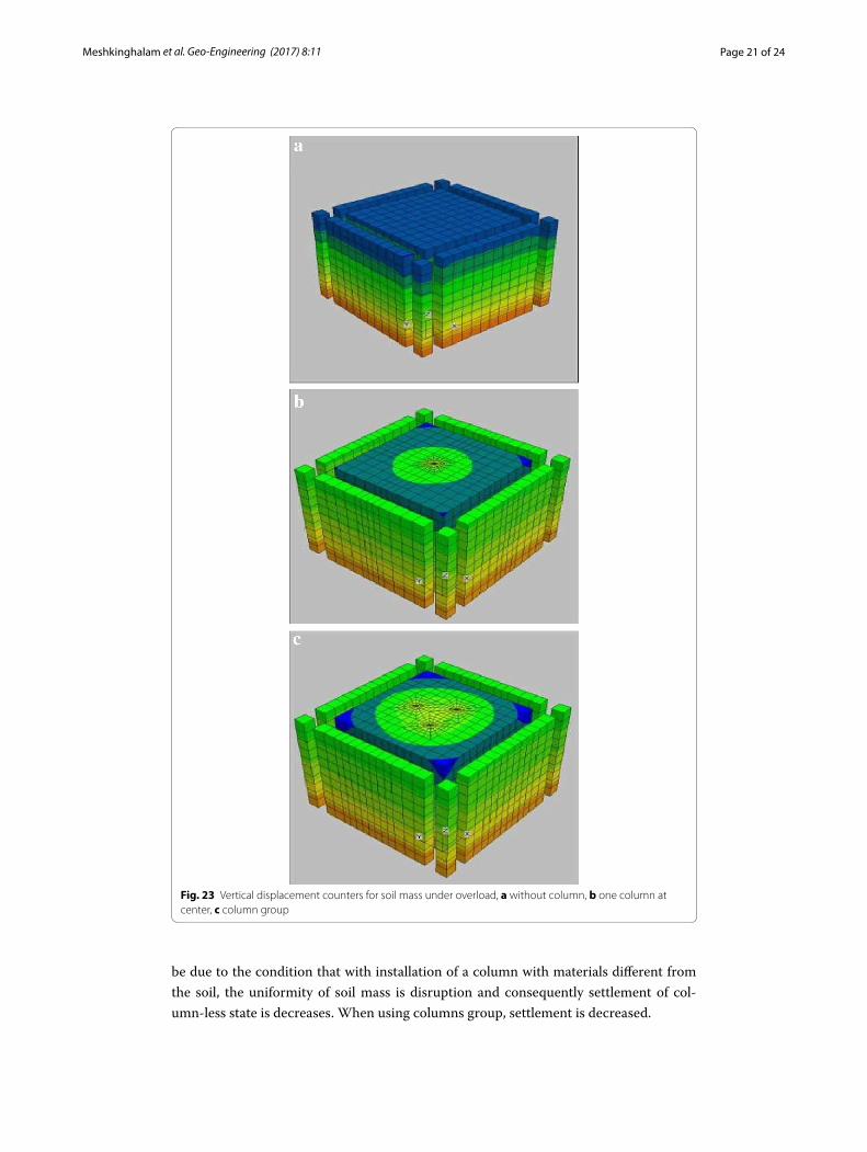
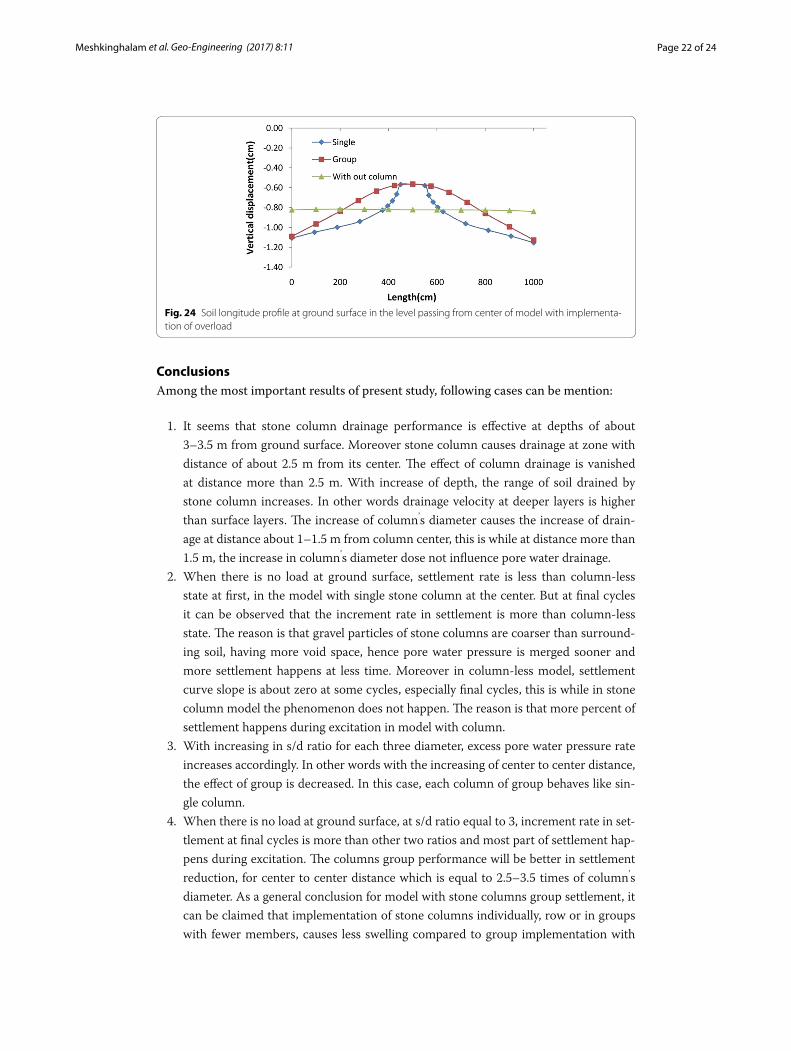
pore water pressure reaches its maximum level. After excess pore water pressure reaches its maximum level, the settlement starts to increase with uniform slope and relative fluc-tuation. Moreover it can be seen that with installation of stone column in the model, the curve of settlement against excess pore water pressure is like column-less state at first, though it has descending procedure with irregular process in less cycles. After excess pore water pressure reached initial value of descending process (second 6), the settle-ment starts to increase with uniform slope and relative oscillation. Comparing diagrams with and without overload, it can be seen that by applying load, settlement fluctuation values are eliminated and settlement amount is not fixed in any cycle, this is while in without load diagrams, settlement is fixed in some cycles, though access pore water pressure of these cycles is downward. The reason is that by applying load, since vertical stress caused by soil mass is present, growth rate of settlement not reaches to zero at cycles and it has an ascending form. Vertical displacement counters of above mentioned model are as Fig. 23. It can be seen that with applying of load, a relatively uniform settle-ment happens at the depth of 1 m from ground surface. And generally the change in set-tlement by depth becomes uniform. The reason for such phenomenon is that total stress and effective stress increase. With installation of a column at the center of the model in a circular area concentric to column, with diameter which is about 2.5 times bigger than column’s diameter, the settlement reduces considerably. The settlement was almost uniform in other areas of model. Soil mass settlement was controlled well with instal-lation of columns group, and this caused considerable decrease of the settlement. Fig-ure 24 shows longitude profile of the soil in ground surface for three above mentioned states. Presented profiles are related to a section passing from the center of the model. It can be seen that vertical displacement of the points at ground surface for state in which soil mass is column-less has almost the same value that this value shows soil mass set-tlement. With installation of single column at the center of the model, settlement value is fixed and decreased in a circular area concentric to column, with diameter which is about 2.5 times bigger than column’s diameter. Outside above mentioned area, the set-tlement increases toward sides, with quiet slope. The reason is that, getting away from above mentioned area, the stone column’s effect (drainage and strength effect) decreases and settlement increases at the sides of model, compared to column-less state. It might

Fig. 22 Changes of vertical displacement against excess pore pressure


be due to the condition that with installation of a column with materials different from the soil, the uniformity of soil mass is disruption and consequently settlement of col-umn-less state is decreases. When using columns group, settlement is decreased.

Fig. 23 Vertical displacement counters for soil mass under overload, a without column, b one column at center, c column group


ConclusionsAmong the most important results of present study, following cases can be mention:

1. It seems that stone column drainage performance is effective at depths of about 3–3.5 m from ground surface. Moreover stone column causes drainage at zone with distance of about 2.5 m from its center. The effect of column drainage is vanished at distance more than 2.5 m. With increase of depth, the range of soil drained by stone column increases. In other words drainage velocity at deeper layers is higher than surface layers. The increase of column’s diameter causes the increase of drain-age at distance about 1–1.5 m from column center, this is while at distance more than 1.5 m, the increase in column’s diameter dose not influence pore water drainage.

2. When there is no load at ground surface, settlement rate is less than column-less state at first, in the model with single stone column at the center. But at final cycles it can be observed that the increment rate in settlement is more than column-less state. The reason is that gravel particles of stone columns are coarser than surround-ing soil, having more void space, hence pore water pressure is merged sooner and more settlement happens at less time. Moreover in column-less model, settlement curve slope is about zero at some cycles, especially final cycles, this is while in stone column model the phenomenon does not happen. The reason is that more percent of settlement happens during excitation in model with column.

3. With increasing in s/d ratio for each three diameter, excess pore water pressure rate increases accordingly. In other words with the increasing of center to center distance, the effect of group is decreased. In this case, each column of group behaves like sin-gle column.

4. When there is no load at ground surface, at s/d ratio equal to 3, increment rate in set-tlement at final cycles is more than other two ratios and most part of settlement hap-pens during excitation. The columns group performance will be better in settlement reduction, for center to center distance which is equal to 2.5–3.5 times of column’s diameter. As a general conclusion for model with stone columns group settlement, it can be claimed that implementation of stone columns individually, row or in groups with fewer members, causes less swelling compared to group implementation with

Fig. 24 Soil longitude profile at ground surface in the level passing from center of model with implementa‑tion of overload


dense meshing. In a certain number of column with decreasing of distance among columns, soil swelling increases.

5. With load applying in column-less model, we will see a relatively uniform settlement till depth of about 1 m from ground surface. And generally changes of settlement at depth will happen uniformly. This is due to the increase of total stress and effective stress, consequently. With installation of a column at the center of model in a circular area concentric with stone column with diameter which is about 2.5 times bigger than column’s diameter, the settlement will be decreased considerably. The settle-ment is almost uniform in other zones. When installing stone columns group, this range is wider.

Authors’ contributionAll three authors participate in the analyses and writting of the paper. All authors read and approved the final manuscript.

Author details1 Department of Civil Engineering, University of Tabriz, Tabriz, Iran. 2 Islamic Azad University Ahar Branch, Ahar, Iran.

Competing interestsThe authors declare that they have no competing interests.

Publisher’s NoteSpringer Nature remains neutral with regard to jurisdictional claims in published maps and institutional affiliations.

Received: 25 October 2015 Accepted: 19 May 2017

References 1. Martin JBG (2004) Quantitative evaluation of stone column techniques for earthquake liquefaction mitigation. In

Proceedings of the tenth world conference on earthquake engineering: 19–24 July 1992, Madrid, Spain. CRC Press, p 1477

2. Shenthan T (2006) Soil densification using vibro‑stone columns supplemented with wick drains. Student Research Accomplishments, p 9

3. Quimby MJ (2009) Liquefaction mitigation in silty sands using stone columns with wick drains 4. Sasaki Y, Taniguchi E (1982) Shaking table tests on gravel drains to prevent liquefaction of sand deposits. Soils Found

22(3):1–14 5. Brennan AJ, Madabhushi SPG (2002) Effectiveness of vertical drains in mitigation of liquefaction. Soil Dyn Earthq

Eng 22(9):1059–1065 6. Adalier K, Elgamal A, Meneses J, Baez JI (2003) Stone columns as liquefaction countermeasure in non‑plastic silty

soils. Soil Dyn Earthq Eng 23(7):571–584 7. Sadrekarimi A, Ghalandarzadeh A (2005) Evaluation of gravel drains and compacted sand piles in mitigating lique‑

faction. Ground Improv 9(3):91 8. Maharjan M, Takahashi A (2013) Centrifuge model tests on liquefaction‑induced settlement and pore water migra‑

tion in non‑homogeneous soil deposits. Soil Dyn Earthq Eng 55:161–169 9. Wang B, Zen K, Chen GQ, Zhang YB, Kasama K (2013) Excess pore pressure dissipation and solidification after lique‑

faction of saturated sand deposits. Soil Dyn Earthq Eng 49:157–164 10. Lu J, Yang Z, Adlier K, Elgamal A (2004) Numerical analysis of stone column reinforced silty soil. In Proceedings of the

15th Southeast Asian geotechnical conference, Bangkok, Thailand, November 23, vol. 26 11. Papadimitriou A, Moutsopoulou ME, Bouckovalas G, Brennan A (2007) Numerical investigation of liquefaction

mitigation using gravel drains. In 4th international conference on earthquake geotechnical engineering 12. Bouckovalas GD, Papadimitriou AG, Niarchos DG, Tsiapas YΖ (2011) Sand fabric evolution effects on drain design for

liquefaction mitigation. Soil Dyn Earthq Eng 31(10):1426–1439 13. Lu MM, Xie KH, Wang SY (2011) Consolidation of vertical drain with depth‑varying stress induced by multi‑stage

loading. Comput Geotech 38(8):1096–1101 14. Walker RT (2011) Vertical drain consolidation analysis in one, two and three dimensions. Comput Geotech

38(8):1069–1077 15. Asgari A, Oliaei M, Bagheri M (2013) Numerical simulation of improvement of a liquefiable soil layer using stone

column and pile‑pinning techniques. Soil Dyn Earthq Eng 51:77–96 16. Castro J, Cimentada A, da Costa A, Cañizal J, Sagaseta C (2013) Consolidation and deformation around stone col‑

umns: comparison of theoretical and laboratory results. Comput Geotech 49:326–337 17. Ni J, Indraratna B, Geng XY, Carter JP, Rujikiatkamjorn C (2013) Radial consolidation of soft soil under cyclic loads.

Comput Geotech 50:1–5


18. Castro J (2014) Numerical modelling of stone columns beneath a rigid footing. Comput Geotech 60:77–87 19. Indraratna B, Ngo NT, Rujikiatkamjorn C, Sloan SW (2015) Coupled discrete element–finite difference method for

analysing the load‑deformation behaviour of a single stone column in soft soil. Comput Geotech 63:267–278 20. Esmaeili M, Hakimpour SM (2015) Three dimensional numerical modelling of stone column to mitigate liquefaction

potential of sands. J Seismol Earthq Eng 17(2):127 21. FLAC3D version 2.1 online manual table of contents 22. Arulmoli K, Muraleetharan KK, Hossain MM, Fruth LS (1992) VELACS: verification of liquefaction analyses by centri‑

fuge studies, laboratory testing program, soil data report. Earth Technol Corpor 332:51–58 23. Taiebat M, Pak A (2004) A fully coupled dynamic analysis of velacs experiment no. 1, using a critical state two‑

surface plasticity model for sands. In Proceedings of the thirteenth world conference on earthquake engineering, Vancouver, BC, Canada. Paper ID, (vol. 2239), p 13

24. Bathe KJ, Wilson EL (1976) Numerical methods in finite element analysis, vol 197. Prentice‑Hall, Englewood Cliffs, NJ 25. Biggs JM (1964) Introduction to structural dynamics. McGraw‑Hill College, New York 26. FHWA (1983) Design and construction of stone column, vol. 1. Report No. FHWA, RD‑83/026

numerical investigation of stone columns system …...numerical investigation of stone columns...

Documents