Numerical Simulation of Bubble Columns by integration of Bubble Cell

Model into the Population Balance Framework

Mopeli Khama

Thesis presented for the degree of

MASTER OF SCIENCE IN CHEMICAL ENGINEERING

Under the supervision of: Assoc. Prof. Randhir Rawatlal

In the Department of Chemical Engineering

UNIVERSITY OF CAPE TOWN

February 2014

The copyright of this thesis vests in the author. No quotation from it or information derived from it is to be published without full acknowledgement of the source. The thesis is to be used for private study or non-commercial research purposes only.

Published by the University of Cape Town (UCT) in terms of the non-exclusive license granted to UCT by the author.

Univers

ity of

Cap

e Tow

n

Plagiarism declaration

“I know the meaning of plagiarism and declare that all the work in the document, save for that which is properly acknowledged, is my own”

Date

Signature

i

Abstract

Bubble column reactors are widely used in the chemicals industry including

pharmaceuticals, waste water treatment, flotation etc. The reason for their wide

application can be attributed to the excellent rates of heat and mass transfer that are

achieved between the dispersed and continuous phases in such reactors. Although

these types of contactors possess the properties that make them attractive for many

applications, there still remain significant challenges pertaining to their design, scale-

up and optimization. These challenges are due to the hydrodynamics being complex

to simulate. In most cases the current models fail to capture the dynamic features of

a multiphase flow. In addition, since most of the developed models are empirical,

and thus beyond the operating conditions in which they were developed, their

accuracy can no longer be retained. As a result there is a necessity to develop

generic models which can predict hydrodynamics, heat and mass transfer over a

wide range of operating conditions.

With regard to simulating these systems, Computational Fluid Dynamics (CFD) has

been used in various studies to predict mass and heat transfer characteristics,

velocity gradients etc (Martín et al., 2009; Guha et al., 2008; Olmos et al., 2001;

Sanyal et al., 1999; Sokolichin et al., 1997).The efficient means for solving CFD are

needed to allow for investigation of more complex systems. In addition, most models

report constant bubble particle size which is a limitation as this can only be

applicable in the homogenous flow regime where there is no complex interaction

between the continuous and dispersed phase (Krishna et al., 2000; Sokolichin &

Eigenberger., 1994). The efficient means for solving CFD intimated above is

addressed in the current study by using Bubble Cell Model (BCM). BCM is an

algebraic model that predicts velocity, concentration and thermal gradients in the

vicinity of a single bubble and is a computationally efficient approach

The objective of this study is to integrate the BCM into the Population Balance Model

(PBM) framework and thus predict overall mass transfer rate, overall intrinsic heat

transfer coefficient, bubble size distribution and overall gas hold-up. The

experimental determination of heat transfer coefficient is normally a difficult task, and

in the current study the mass transfer results were used to predict heat transfer

coefficient by applying the analogy that exists between heat and mass transfer. In

ii

applying the analogy, the need to determine the heat transfer coefficient

experimentally or numerically was obviated. The findings indicate that at the BCM Re

numbers (Max Re= 270), there is less bubble-bubble and eddy-bubble interactions

and thus there is no difference between the inlet and final size distributions. However

upon increasing Re number to higher values, there is a pronounced difference

between the inlet and final size distributions and therefore it is important to extend

BCM to higher Re numbers.

The integration of BCM into the PBM framework was validated against experimental

correlations reported in the literature. In the model validation, the predicted

parameters showed a close agreement to the correlations with overall gas hold-up

having an error of ±0.6 %, interfacial area ±3.36 % and heat transfer coefficient

±15.4 %. A speed test was also performed to evaluate whether the current model is

quicker as compared to other models. Using MATLAB 2011, it took 15.82 seconds

for the current model to predict the parameters of interest by integration of BCM into

the PBM framework. When using the same grid points in CFD to get the converged

numerical solutions for the prediction of mass transfer coefficient, the computational

time was found to be 1.46 minutes. It is now possible to predict the intrinsic mass

transfer coefficient using this method and the added advantage is that it allows for

the decoupling of mass transfer mechanisms, thus allowing for more detailed

designs. The decoupling of mass transfer mechanisms in this context refers to the

separate determination of the intrinsic mass transfer coefficient and interfacial area.

iii

Acknowledgements

I am very thankful for my supervisor, Assoc. Prof. Randhir Rawatlal, for his constant

support and guidance which always ignited zeal and enthusiasm in me, and sparked

further my interest of working towards the completion of the project. As we journeyed

through the project, he instilled into me some incredible skills in modelling and

technical writing, for this I am heavily indebted to him.

I am grateful for my family members and friends who motivated me and helped me to

endure to the completion of the project. Kea lea leboha Maphuthing

I would like to thank DST-NRF Centre of Excellence in Catalysis for financial

support.

iv

Table of Contents 1. Introduction .................................................................................................................................... 1

1.1. Background to investigation ................................................................................................... 1

1.2 Predicting hydrodynamic properties ...................................................................................... 2

1.3 Modelling bubble column hydrodynamics ............................................................................. 5

1.4 Summary ................................................................................................................................. 7

2. Literature review ............................................................................................................................. 8

2.1. Prediction of hydrodynamics in bubble columns ................................................................... 8

2.1.1. Mass transfer coefficient ................................................................................................ 8

2.1.2. Interfacial area .............................................................................................................. 10

2.1.3. Mean bubble diameter ................................................................................................. 11

2.1.4. Bubble size distribution ................................................................................................ 11

2.1.5. Gas hold-up ................................................................................................................... 12

2.1.6. Bubble rise velocity ....................................................................................................... 13

2.1.7. Heat transfer coefficient ............................................................................................... 13

2.1.8. Heat and mass transfer analogy ................................................................................... 15

2.1.9. Application to bubble columns ..................................................................................... 18

2.2. Computational fluid dynamics .............................................................................................. 19

2.2.1. Governing equations for fluid flow ............................................................................... 19

2.2.2. Finite volume method ................................................................................................... 22

2.3. Population Balance Modelling .............................................................................................. 23

2.2.3. Coalescence .................................................................................................................. 24

2.2.4. Break up ........................................................................................................................ 29

2.3. Incorporating Population Balance into CFD .......................................................................... 34

2.6. Experimental work on investigating the hydrodynamics in bubble columns ....................... 37

2.4. Summary of literature review ............................................................................................... 39

3. Research objectives and key questions ........................................................................................ 41

3.1. Research objectives .............................................................................................................. 41

3.2. Hypothesis ............................................................................................................................. 42

3.3. Key questions ........................................................................................................................ 42

4. Model development...................................................................................................................... 43

4.1. Bubble Cell Model ................................................................................................................. 44

4.1.1. Bubble rise velocity ....................................................................................................... 49

4.1.2. Boundary conditions ..................................................................................................... 51

v

4.2. Numerical estimation of heat and mass transfer coefficients .............................................. 53

4.2.1. Heat and mass transfer analogy ................................................................................... 56

4.3. Population Balance Model .................................................................................................... 58

4.3.1. Coalescence model ....................................................................................................... 61

4.3.2. Break up model ............................................................................................................. 62

4.3.3. A solution to the Population Balance Equation ............................................................ 64

4.4. Numerical estimation of overall heat and mass transfer coefficients .................................. 70

4.5. Numerical stability and convergence .................................................................................... 71

4.5.1. Size range and meshing ................................................................................................ 71

4.6. Model Consistency checks .................................................................................................... 72

4.6.1. Volume balance: ........................................................................................................... 72

4.7. Consistency checks on the Population Balance Model ......................................................... 74

4.8. Model consistency checks on total mass transfer ................................................................ 76

4.9. The model speed test ............................................................................................................ 77

5. Results and discussion .................................................................................................................. 78

5.1 Spatial variation of Bubble size distribution at low Reynolds number ................................. 80

5.2 Bubble size distribution at high Reynolds number ............................................................... 81

5.3 Overall mass transfer rate..................................................................................................... 84

5.3.1 The relationship between the bubble size, axial position and the mass transfer

coefficient ..................................................................................................................................... 86

5.4 Sensitivity analysis ................................................................................................................ 88

5.4.1 The influence of column dimensions on gas hold-up ................................................... 88

5.4.2 The influence of inlet bubble size on the predicted gas hold up .................................. 91

5.4.3 The influence of column diameter on predicted gas-liquid interfacial area and the

number of bubbles ........................................................................................................................ 92

5.4.4 The influence of the expansion term on the predicted mean diameter ...................... 94

5.5 Predicting heat transfer coefficients..................................................................................... 96

5.6 Model validation ................................................................................................................... 98

5.6.1 Validating gas hold-up................................................................................................... 99

5.8.2 Validating interfacial area ........................................................................................... 100

5.8.3. Validating heat transfer coefficient ............................................................................ 101

5.8.4 Validating mass transfer results .................................................................................. 102

5.9 Model speed test ................................................................................................................ 103

5.10 Summary ............................................................................................................................. 103

vi

6. Concluding remarks .................................................................................................................... 104

6.1. Recommendations .............................................................................................................. 106

7. References .................................................................................................................................. 108

List of Figures

Figure 1 Schematic diagram of a bubble column reactor. ............................................................. 2

Figure 2: Flow regimes in a 3-D bubble column (Chen et al., 1994). (a), Bubbly flow regime; (b), Transition flow regime; (c), Churn turbulent flow regime ...................................................... 14

Figure 3: Schematic diagram of heat transfer Probe. 1, Teflon tube; 2, brass shell;3,heat flux sensor;4,heater;5,Teflon cap(Wu, Cheng Ong & Al-Dahhan., 2001) ......................................... 15

Figure 4: CFD bubble column simulation approaches depending on length scale (Zhang, 2007) .................................................................................................................................................... 19

Figure 5: Mechanism for bubble coalescence. V1 and V2 are bubble volumes and h(r,t) is the liquid film thickness and hcritical is the critical film thickness(Prince & Blanch, 1990a). ...... 27

Figure 6: death and birth due to coalescence of bubbles (simulated from the model by Saffman and Turner (1956)) ............................................................................................................. 29

Figure 7: death and birth due to coalescence of bubbles (simulated from the model by Prince & Blanch (1990))................................................................................................................................. 29

Figure 8: mechanism for bubble binary breakage through collision with a turbulent eddy (Hinze, 1955). ..................................................................................................................................... 30

Figure 9: death and birth due to breakage of bubbles (simulated from the model by Patruno et al. (2009)) ........................................................................................................................................ 32

Figure 10: death and birth due to breakage of bubbles (simulated from the model by Luo & Svendsen., (1996))............................................................................................................................. 33

Figure 11: Mass transfer coefficient predicted from correlating Re with Sh and Re with δ .... 47

Figure 12: Concentration (δc) and thermal (δt) boundary layers ................................................. 49

Figure 13: Bubble rise velocity as calculated from macroscopic force balance ....................... 51

Figure 14: Mesh generation for the system under study .............................................................. 52

Figure 15: The CFD methodology for approximating mass transfer coefficient ....................... 53

Figure 16: Concentration boundary layer in the vicinity of a single bubble at various Reynolds number ............................................................................................................................... 57

Figure 17: Thermal boundary layer in the vicinity of a single bubble at various Reynolds number ................................................................................................................................................. 57

Figure 18: heat transfer coefficient prediction by analogy and CDF determination ................ 58

Figure 19: Representation of Particle size distribution by the discrete method........................ 65

Figure 20: A schematic diagram of a bubble column ................................................................... 67

Figure 21: mass transfer coefficients results from BCM .............................................................. 70

Figure 22: Mass transfer coefficient for a population of bubbles ............................................... 70

Figure 23: The grid dependence of the predicted Nusselt number ............................................ 72

Figure 24: weighted mean for bubble size distribution for two different column compartments chosen (2 and 4)................................................................................................................................. 76

Figure 25: A schematic diagram on how BCM was integrated into the PBM framework ........ 56

Figure 26: Bubble size distribution at low Re numbers (max Re=270) ...................................... 81

Figure 27: bubble size distribution along the column height ........................................................ 82

Figure 28: Inlet and final size distributions (column height =2 m) .............................................. 83

vii

Figure 29: Inlet and final size distributions (column height =3 m) .............................................. 83

Figure 30: Mass transfer coefficient in the vicinity of a single bubble at various Re numbers .............................................................................................................................................................. 85

Figure 31: Intrinsic mass transfer coefficient at various column compartments ....................... 87

Figure 32: Bubble Averaged mass transfer coefficient at various column compartments ...... 87

Figure 33: Local mass transfer coefficient in the vicinity of individual bubbles ........................ 88

Figure 34: bubble size distribution with the inclusion of mass transfer term in the bubble PBM equation (Max Re=7616) .................................................................................................................. 95

Figure 35: bubble size distribution with the exclusion of mass transfer term in the bubble PBM equation (Max Re=7616) ......................................................................................................... 96

Figure 36: The effect of bubble size on heat transfer coefficient ................................................ 97

Figure 37: The variation of heat transfer coefficient along the column height at bigger bubbles chosen as initial sizes (minimum size (7.3 mm) and maximum size (1.2 cm)) .......... 98

Figure 38: The variation of heat transfer coefficient along the column height at smaller bubbles chosen as initial sizes (minimum size (0.73 mm) and maximum size (1.2 mm)) ...... 98

Figure 39: Comparison of the model results to the correlation results ...................................... 99

List of Tables

Table 1: Mathematical expressions to show the similarity between heat and mass transfer . 16

Table 2: Mass transfer coefficient predicted at various Re numbers ......................................... 46

Table 3: Concentration boundary layer predicted at various Re numbers ............................... 48

Table 4: Volumetric flowrate along the column compartments without mass transfer consideration ....................................................................................................................................... 74

Table 5: Volumetric flow-rate along the column compartments with mass transfer consideration ....................................................................................................................................... 75

Table 6: Total gas volume along the column compartments ....................................................... 75

Table 7: Volume balance with mass transfer consideration ........................................................ 76

Table 8: The relationship between the global and local variables .............................................. 80

Table 9: Overall compartment mass transfer rate along the column compartments ............... 85

Table 10: Gas hold up predicted at different column diameters ................................................ 90

Table 11: Gas hold up predicted at different column heights with the same diameter (0.15 m) .............................................................................................................................................................. 91

Table 12: Gas hold up predicted at different initial bubble sizes ................................................ 92

Table 13: Interfacial area predicted at different column diameters ............................................ 93

Table 14: Interfacial area predicted at different column heights ................................................. 94

Table 15: Number of bubbles predicted at different column diameters ..................................... 94

Table 16: The predicted Sauter mean diameter with and without mass transfer consideration .............................................................................................................................................................. 95

Table 17: Validating interfacial area (bubble sizes ranging from 7.3 mm to 1.2 cm) ............. 100

Table 18: Validating interfacial area (bubble sizes ranging from 2.4 mm to 8.8 mm) ........... 101

Table 19: Validating the Nusselt number calculated from the model against correlations ... 102

Table 20: Validation of mass transfer results ............................................................................... 103

viii

Nomenclature A Area of transfer (m2)

ap Specific interfacial area (m2/m3)

BCM Bubble Cell Model

CB Dimensionless constant

CAb Gas concentration in the bulk liquid (mol/m3)

CA0 Initial gas concentration (mol/m3)

CAs Gas concentration at the gas-liquid interface (mol/m3)

CD Drag coefficient

cf Coefficient of surface area increase

CL lift force coefficient

CVM virtual mass coefficient

d Diameter (m)

ds Sauter mean diameter (m)

DAB Mass diffusivity (m2/sec)

DNS Direct Numerical Simulation

ê Internal energy (kJ/kg)

F Forces acting on the control volume

f Probability number density

FD Drag force (N)

FG Gravity force (N)

F L Lift force (N)

FVM virtual mass force (N)

𝙜 Gravitational acceleration (m2/sec)

hc Heat transfer coefficient (W/m2.K)

k Thermal conductivity (W/m.K)

kL Intrinsic mass transfer coefficient (m/sec)

ix

kLa Volumetric mass transfer coefficient (1/sec)

Ntot overall mass transfer rate (mol/sec)

Nu Nusselt number

Nb total number of bubbles

nx Component of the unit normal vector in x-direction

ny Component of the unit normal vector in y-direction

Unit normal vector at the surface

P Total pressure (Pa)

PBM Population Balance Model

PC Coalescence collision frequency

PDE Partial differential equation(s)

Pr Prandtl number

q Heat flow rate (J/sec)

rA Mass transfer rate (mol/sec)

rC Rate of bubble coalescence

rB Rate of bubble break-up

Re Reynolds number

Ś Internal energy generated within the fluid control volume

Sc Schmidt number

Sh Sherwood number

T Temperature (K)

Ts surface temperature (K)

tij Time needed for coalescence of bubbles (sec)

Bulk temperature (K)

u x direction velocity (m/sec)

Ur Bubble rise velocity (m/sec)

V Total resultant magnitude of velocity

v y direction velocity (m/sec)

x

ν Kinematic viscosity (m2/sec)

Velocity vector with the components u and v

We Weber number

Greek symbols

α Thermal diffusivity (m2/sec)

σ Surface tension of a sphere

τ Shear stress (N/m2)

Contact time for the bubbles (sec)

𝛅c Concentration boundary layer (m)

𝛅t Thermal boundary layer (m)

µ Dynamic viscosity (kg/m.sec)

εg Gas hold-up

ε Turbulent energy dissipation rate (m2/sec3)

ΩB Breakup rate (m-3s-1)

ῼc Coalescence rate (m-3s-1)

θijT Turbulent collision rate (m-3s-1)

θijB Buoyancy driven collision rate (m-3s-1)

θijLS Laminar shear collision rate (m-3s-1)

Critical diameter (dimensionless)

Subscripts

s Surface

g Gas

t Temperature

c Concentration

D Drag

xi

L Lift

Vm Virtual mass

x x-direction

y y-direction

Superscripts

B Buoyancy

Ls Laminar shear

T Turbulence

1

Chapter 1

1. Introduction

1.1. Background to investigation

A bubble column is a vessel through which a gas is introduced at the base through a

sparger as illustrated in Figure 1. The gas bubbles make up the dispersed phase,

while the liquid constitutes a continuous phase which could be flowing or stagnant.

The bubbles rise at varying velocities depending on their size and the proximity of

other bubbles which may influence the motion of the entire bubble population. The

bubble rise velocity is an important parameter in characterising the bubble column

hydrodynamics.

Bubble columns are extensively used in a wide range of industrial applications such

as flotation, petrochemical, biochemical and chemical. The reasons for their wide

application are the high rates of heat and mass transfer, ease of operation, low

maintenance costs and the absence of moving parts. The mode of operation in

bubble column reactors can be either continuous or semi-batch. In the continuous

mode of operation, both the gas and the liquid flow concurrently upward in the

column. On the other hand, for the semi-batch mode of operation, the liquid is

stagnant and the gas is introduced at bottom of the column in the form of bubbles. In

the current work, the latter mode of operation was considered when modelling the

hydrodynamics in the column.

Although the internal structure of the column is simple, the hydrodynamics are

complex. For the improved design and scale-up, an understanding of multiphase

fluid dynamics and its influences in the flow field is essential. The hydrodynamic

variables that influence the operation, performance, design and scale up are gas

hold-up, Sauter mean diameter, and interfacial area and bubble size distribution. In

view of the importance of the accurate prediction of the aforementioned

hydrodynamic variables, the present work is aimed at developing a reliable predictor

for these variables.

2

Figure 1 Schematic diagram of a bubble column reactor.

1.2 Predicting hydrodynamic properties

The bubble rise velocity is an important parameter in characterising the bubble

column hydrodynamics. It is normally calculated from force balances over each

particle using Newton’s second law of motion as reported by Delnoij et al. (1997).

The forces that are considered to be acting on a spherical, non-deformable bubble

are drag, and lift, virtual or added mass, pressure and gravity. The force balance

allows for bubble acceleration, which in turn allows for the determination of bubble

velocity. The bubble rise velocity affects the hydrodynamics, in the sense that at low

velocities, break up and coalescence are negligible due to less bubble-bubble

interactions or eddy-bubble collision. At the low velocities, the bubble residence time

also increases and thus high gas hold-up is expected.

However, at high bubble velocities, break up and coalescence begin to take place as

there are more frequent interactions between bubbles and the continuous phase,

and between the bubbles themselves. In this case, the bubble residence time is

small and big bubbles are expected due to the interaction that takes place. It is

expected that gas hold-up will decrease due to decreased residence time.

3

The accurate prediction of gas hold-up is of paramount importance due to its

significant impact on the performance of bubble columns. The prediction of mean

diameter and gas hold-up allows for the prediction of gas the liquid interfacial area,

and as a result allows for the calculation of heat and mass transfer rates between the

phases (Jamialahmadi & Müuller-Steinhagen, 1993). The gas-liquid interfacial area

can be calculated from mean diameter and gas hold-up as shown in Equation (1.1).

The bubble mean diameter can be calculated from the predicted size distribution

using number density probability distribution and bubble size as illustrated in

Equation (1.2). The spatial variation in the column leads to pressure variation which

in turn results in liquid recirculation. The rate of mixing, the heat and mass transfer

rates are all dictated by liquid recirculation in the column (Wu, Cheng Ong & Al-

Dahhan, 2001). There are various techniques used for the determination of local gas

hold-up in bubble columns, namely: computed tomography, particle image

velocimetry, optical fibre probes and gamma-ray attenuation.

(1.1)

∑

∑

(1.2)

In the characterization of hydrodynamics in bubble columns, Bouaifi et al. (2001)

stated that the separation of mass transfer coefficient and interfacial area is of

paramount importance. The separation is crucial as the volumetric mass transfer

coefficient (in its lumped form), does not allow for decoupling mass transfer

mechanisms. It was explained that the Independent determination of the intrinsic

mass transfer coefficient and interfacial area, into the intrinsic mass transfer

coefficient and specific interfacial area allows for an investigation to determine which

parameter controls mass transfer. According to the research of Bouaifi et al. (2001),

in the determination of the volumetric mass transfer coefficient, two columns were

used for the experiments. Their findings indicated that in one of the columns, the

volumetric mass transfer coefficient was found to be dependent on interfacial area

only. In the other column it was found that, the volumetric mass transfer coefficient

4

was not dependent on interfacial area, as three different spargers which resulted in

different interfacial areas were used, but the volumetric mass transfer coefficient

found in each case was the same. It was concluded that the liquid mass transfer

coefficient is dependent on operating conditions such as gas velocity and sparger

type. The findings justified the need to independently determine the two parameters

(intrinsic mass transfer coefficient and specific interfacial area) for a better

understanding of mass transfer mechanisms, and the current work aimed at

separating the two parameters for a better analysis.

The liquid phase properties have an impact on the formation of bubbles in the bubble

column and thus they affect the gas hold-up (Kantarci, Borak & Ulgen, 2005). To

investigate this phenomenon, the liquid phase viscosity was changed and its impact

on the predicted hydrodynamics parameters was determined. It is reported in the

literature that upon increasing liquid viscosity, larger bubbles are formed and thus

low gas hold-up and high rise velocities are attained. The effect of operating

conditions like pressure and temperature on the predicted hydrodynamics have also

been reported in the literature (Kantarci, Borak & Ulgen, 2005), but the current study

did not investigate their influence on the hydrodynamics.

Bubble size is also an important parameter in the characterization of bubble column

hydrodynamics. It affects gas hold-up, interfacial area and bubble rise velocity. The

development of a model that predicts bubble size as a function of position and time

in the column, can aid in the prediction of these parameters that are dependent on it.

The Population Balance Model is therefore used in the prediction of bubble size

distribution and its impact in the flow field is determined from Computational Fluid

Dynamics.

Kantarci et al. (2005) stated that for high conversion levels, larger reactor heights

and diameters are desired due to large gas throughputs. They also stated that the

use of longer and larger diameter columns do not allow for an ease of operation, and

as a result an optimization process is required. It is therefore necessary to devise

some optimization tools for the design of a column that is easy to operate by

reducing the diameter and length of the column while still maintaining the best

results. For this to be achieved, the hydrodynamic variables that influence the

5

performance of the column have to be accurately predicted, and the optimum

operating conditions can be determined thereof.

1.3 Modelling bubble column hydrodynamics

Over the past years Computational Fluid Dynamics (CFD) has been used for

simulation of bubble column reactors. CFD is a tool that solves Navier Stokes

equations that describe fluid flow numerically. Simulation by CFD is based on Euler-

Euler, Euler-Lagrange and Direct Numerical simulation (DNS). All the

aforementioned simulation techniques are computationally expensive and require

high performance computing hardware. In most simulations, the constant particle

size assumption is used (Krishna et al., 2000; Sokolichin & Eigenberger., 1994),

which is a limitation as this could only be applicable in homogenous flow regime

where there is no complex interaction between the continuous and dispersed phase.

In the cases where flow regime changes and there is complex interaction between

the two phases, CFD has to be coupled with the Population Balance Model for a

better understanding of different flow regimes and bubble characteristics in bubble

columns design, scale up and optimization.

Euler-LaGrange treats the liquid phase in the Eulerian representation and the

dispersed phase in the Lagrangian representation by tracking each individual fluid

element in the reactor. In the Euler-Euler approach both the liquid and dispersed

phase are treated in the Eulerian representation (Kantarci, Borak & Ulgen, 2005).

Since Euler-Lagrange tracks each individual fluid element of the dispersed phase, it

requires high computational memory and speed. In terms of computational expense,

it is more expensive than Euler-Euler approach.

Coetzee et al. (2011) developed a novel approach which aims at reducing

computational expense by predicting the flow patterns around single bubbles with an

algebraic flow model dependant on Reynolds number. The model is named Bubble

Cell Model (BCM). In its current development BCM predicts velocity vector fields in

the vicinity of single bubbles and can be extended to predicting thermal and

concentration gradients. Since BCM is a computationally efficient approach, in the

current study, BCM was integrated into the Population Balance framework to predict

concentration gradients and total mass transfer rate in the reactor. Upon the

determination of mass transfer coefficient, the analogy between heat and mass

6

transfer was used to predict heat transfer coefficient, thus a need to develop a model

specifically for predicting heat transfer coefficient was obviated. The Population

Balance Model was validated with mass and heat integration against the empirical

correlations.

The Population Balance is the mathematical framework used in particulate systems

to predict property distribution of discrete entities such as gas bubbles and oil

droplets. It has been used in a wide range of topics, which includes dispersed

phases such as solid-liquid dispersion, liquid-liquid, gas-liquid, and gas-solid

dispersions (Guha et al., 2008; Olmos et al., 2001; Sanyal et al., 1999; Sokolichin

et al., 1997; Sokolichin & Eigenberger, 1999). The general form of the Population

Balance equation is an integro-differential equation in time, space and internal

coordinates (mass, volume and bubble diameter) (Ramkrishna, 2000). The

Population Balance models predict particle size distribution by discretising the size

range, and therefore resulting in a system of differential equations that describe the

rate of accumulation or loss of particle number or mass in each of the size classes.

A Population Balance may include the birth and death terms due to coalescence and

break-up. The robust models are needed for coalescence and break-up in order to

have a good understanding of their impact in size distribution. Due to the complexity

in the behaviour of coalescence and break-up phenomena, there are no analytical

solutions and thus a numerical solution is needed. The bubble size changes due to a

number of phenomena including coalescence, breakup and mass transfer into the

liquid phase. A Population Balance Equation is shown in Equation (1.3) with the

aforementioned phenomena represented in specific terms.

(

)

∫

∫

(

)∫

∫

(1.3)

7

The terms on the left side of the equation represent convective transport; the first

term on the right represents gas expansion due to mass transfer and density

changes. The second and third terms represent break up of bubbles of a larger

volume and break-up of bubbles of volume v. The fourth and fifth terms represent the

coalescence of small bubbles and bubbles of volume v with all other sizes

(Sporleder, Dorao & Jakobsen, 2011)

Most studies in the literature couple the Population Balance Model with Euler-Euler

for simulation of bubble column reactors. In the current study, the Population

Balance Model was used to calculate the bubble size evolution and its impact in the

flow field was computed from its coupling with BCM. The system under study is an

air-water at bubbly flow and the liquid phase was assumed to be clean without

surfactants as they affect bubble break up and coalescence (Lehr, Millies & Mewes,

2002).

1.4 Summary

Although bubble columns have simple internal structure, their modelling can be

complicated by their complex flow structure. The flow structure is complicated by

back-mixing, circulation of bubbles, complex interactions between the phases, and

the bubble shapes which change with the change in flow regime. One example is the

flow structure near the wall region. At this region, the flow is complicated as some of

the bubbles circulate with the liquid as the flow is directed downwards. As a result

the bubble residence time is not directly related to the bubble rise velocity. It is

therefore difficult to develop models that capture the dynamic features of the

multiphase flow and the physics is also not well understood. The behaviour of gas-

liquid contactors is highly inhomogeneous and this is due to the previously

mentioned phenomena. As a result, for modelling these types of reactors, a model

must comprise a Population Balance Equation to predict the distribution of the

dispersed phase and a multi-fluid model to model the flow field. Such a model is

complex and requires significant computational time.

.

8

Chapter 2

2. Literature review

2.1. Prediction of hydrodynamics in bubble columns

The design, scale up and optimization of bubble columns depend on the accurate

prediction of the hydrodynamic parameters. The predicted variables are gas hold-up,

interfacial area, Sauter mean diameter, and heat and mass transfer coefficients.

Over the past decades there has been a considerable research in both modelling

and experiments for the determination of the aforementioned variables. Despite the

significant effort employed, there still remains a challenge to develop models that are

generic in their predictive capability, as most of the work involves empirical

correlations which are limited in their usage (Michele & Hempel, 2002; Pohorecki et

al., 2001). The limitation is brought about by the fact that the correlations used

depend more on equipment type, equipment geometry and operating conditions, and

thus beyond the conditions under which they were developed, accuracy is no longer

achieved.

The literature review presented below considers the state of research in the

modelling of bubble columns, and identifies areas requiring further investigation.

2.1.1. Mass transfer coefficient

Mass transfer refers to the relative motion of species from one phase, stream or

component to another due to concentration gradients. In gas-liquid contactors, mass

transfer from the dispersed to the continuous phase is the primary goal of the

process. The mass transfer rate in these systems depends on bubble size

distribution, turbulent energy dissipation, bubble slip velocity, bubble coalescence

and breakup (Wang, 2010). The CFD-PBM coupled models become attractive tools

in modelling hydrodynamics in bubble columns as they quantitatively account for the

mentioned parameters that affect the mass transfer rate .For gas-liquid systems, the

resistance to mass transfer from one phase to another is often in the liquid phase. In

Bubble columns; the mass transfer rate is the limiting stage of the processes that

take place. The mass transfer rate in gas-liquid systems is calculated from mass

9

transfer coefficient, which is the ratio of the mass transferred to the driving force

(Azzopardi et al., 2011). For this reason the mass transfer coefficient and the specific

interfacial area are normally the distinctive design parameters (Bhole, Joshi &

Ramkrishna, 2008). The total mass transferred from one phase to another can be

taken to be directly proportional to the concentration gradient and gas-liquid

interfacial area. The proportionality constant is taken to be the intrinsic mass transfer

coefficient (kL). The total mass transfer rate is calculated as shown in Equation (2.1).

(2.1)

Over the decades there has been a considerable amount of work done on mass

transfer in bubble columns (Bouaifi et al., 2001; Chaumat et al., 2005; Colombet et

al., 2011; Ferreira et al., 2012; Haut & Cartage, 2005; Kantarci, Borak & Ulgen,

2005; Kerdouss et al., 2008; Krishna & van Baten, 2003; Lau, Lee & Chen, 2012;

Lemoine et al., 2008; Miller, 1983; Moo-Young & Kawase, 1987; Muroyama et al.,

2013; Wang & Wang, 2007; Yeoh & Tu, 2004).

Krishna & van Baten, (2003) developed a CFD model that characterises the

hydrodynamics and mass transfer for an air-water bubble column operating in

heterogeneous and homogeneous flow regimes. In their work, for a heterogeneous

flow regime, the bubbles were classified into two bubble classes, small and large

bubbles. The findings show that for a homogeneous flow regime, the mass transfer

coefficient decreases with the column diameter and that is attributed to an increase

in liquid circulation which increases the velocity of bubbles. As such, a reduced gas-

liquid contact time is realised. The results for mass transfer in a heterogeneous flow

regime showed that it is important to incorporate the effect of bubble break-up and

coalescence through Population Balance Modelling.

Martín et al., (2009) developed a theoretical model to study the effect of bubble

deformation on the mass transfer rate for an air-water system. In their work, the

Population Balance Model was coupled with a theoretical model for Sherwood

number from which the mass transfer coefficient was predicted. Their findings

indicate that in bubble columns, the concentration profiles in the vicinity of individual

bubbles are not entirely developed. This is attributed to the proximity of other

10

bubbles where the concentration of the dissolved gas in the liquid from the individual

bubble, is not only dependent on the total mass transfer from that respective bubble,

but depends also on the mass transfer from other bubbles. As a result it was found

that the mass transfer coefficient in a case of a bubble swarm is smaller compared to

mass transfer coefficient for a single bubble.

Ferreira et al., (2012) used image analysis technique combined with discriminant

factorial analysis for characterisation of hydrodynamics and mass transfer in a

bubble column. Their method allowed for an online and automatic characterisation of

individual bubbles and as a result an accurate prediction of bubble size and specific

interfacial area over a wide range of operating conditions was achieved. The

influence of operating conditions such as liquid phase properties (viscosity and

surface tension), temperature, and type of sparger on the liquid side mass transfer

coefficient were investigated. The findings in their study indicate that the influence of

viscosity on interfacial area and liquid side mass transfer coefficient is considerable.

Temperature was found to have a pronounced influence on mass transfer coefficient

while its influence on specific interfacial area was found to not be significant

2.1.2. Interfacial area

Gas-liquid interfacial area is the area available for mass transfer from one phase to

the other phase. To enhance the rate of heat and mass transfer, the interfacial area

should be large and that is achieved when for the given mass of gas, the bubbles are

small in size. The interfacial area is calculated from the area of the bubbles and their

number densities. The averaging is done as seen in Equation (2.2).

∫

(2.2)

Where N is the total number of bubbles, d is bubble diameter, f is the bubble number

density probability distribution, and V is volume of the column.

For the accurate prediction of the gas–liquid interfacial area, it is apparent that the

bubble Population Balance Equation (PBE) is accurately solved. This can be

attributed to the fact that the gas-liquid interfacial area is calculated from bubble size

and the bubble size distribution is predicted by the PBE. The interfacial area

11

changes to a great degree with the variation in the number density distribution due to

coalescence and breakup. Since the Population Balance Equation estimates bubble

size distribution locally, interfacial area can also be estimated locally throughout the

column (Bannari et al., 2008).

2.1.3. Mean bubble diameter

Bubble size is an important hydrodynamic variable that needs to be accurately

predicted as it affects bubble rise velocity, gas hold-up, interfacial area and ultimately

the rates of heat and mass transfer. The mean bubble diameter is calculated from

the bubble number density probability distribution and bubble size. The number

density probability distribution and bubble size are found from the bubble Population

Balance Equation. It is vital to accurately model the Population Balance Equation as

the accurate prediction of mean diameter depends on how accurate the Population

Balance Equation is modelled. According to Chen et al., (2004), the bubble mean

diameter is calculated as presented in Equation (2.3).

∑

(2.3)

2.1.4. Bubble size distribution

The size of bubbles in the column differs from the initial bubble size of bubbles that

just left the sparger. This difference is attributed to breakup and coalescence that

take place in the column, and the size of the bubbles is mainly dependent on the

balance that is achieved between coalescence and break-up rates (Atika & Yoshida,

1973). In the characterisation of hydrodynamics in bubble column, bubble size

distribution is one of the important characteristics. Bubble size distribution is

dependent on the operating conditions, sparger type, column geometry and physio-

chemical properties of both the continuous and dispersed phase (Bannari et al.,

2008). In order to enhance mass transfer between the two phases, small bubbles

and narrow bubble size distribution over the equipment cross-section are desired.

This can be ascribed to the fact that smaller bubbles render a larger interfacial area,

hence high mass transfer rates. Spatially, the bubble size distribution is not constant

12

in the column due to bubble-bubble interaction and eddy-bubble interaction, and it is

therefore vital to compartmentalise the column and predict size distribution at each

column compartment. In doing so, it can be investigated and confirmed as to

whether bubble size distribution varies along the column. In the present work, the

column was compartmentalised to investigate the aforementioned phenomenon and

also to predict the other hydrodynamic parameters at each compartment.

The importance of bubble size distribution also extends to prediction of flow regime

transition. Wang et al. (2005) developed a theoretical model for the prediction of flow

regime transition based on size distribution. In addition, bubble size distribution

regulates bubble rise velocity, bubble residence time, gas hold-up, the interfacial

area, and hence gas-liquid mass transfer rate (Shimizu et al., 2000).

2.1.5. Gas hold-up

Gas hold-up is defined as the volume fraction of the gas in the gas-liquid dispersion.

It is an important parameter in the optimization, design and scale-up of bubble

column (Moo-Young & Kawase, 1987). It is asserted that it indirectly governs the

liquid phase flow, and ultimately the rates of mixing, heat and mass transfer (Wu,

Cheng Ong & Al-Dahhan, 2001). There has been extensive work both theoretically

and experimentally for determination of gas hold-up. In the current work, gas hold-up

was predicted from mean diameter and interfacial area both of which are predicted

from the Population Balance Equation. The gas hold-up is calculated as shown in

Equation (2.4)

(2.4)

Alternatively, gas hold-up can be calculated from total number of bubbles and

number density probability distribution as illustrated in Equation (2.5).

∫

(2.5)

13

2.1.6. Bubble rise velocity

Bubble rise velocity is one of the most important parameters that govern the

performance of a bubble column reactor. The aforementioned hydrodynamic

variables such as gas hold-up and interfacial are influenced by bubble rise velocity;

because bubble rise velocity dictates how much time a bubble spends in the column.

At higher rise velocities, which are experienced in the case of large bubbles, the gas

hold-up becomes small due to reduced residence time. The interaction of bubbles

amongst themselves is also influenced by the rate at which they rise in the column.

At low rise velocities, there is less bubble-bubble interaction and it is expected that

the bubble size distribution will be narrow. The macroscopic force balance is used to

calculate the velocity of each bubble and the expression for the force balance is

illustrated in section (4.1.1)

The interaction between the continuous and the dispersed phase affects the

abovementioned interphase forces. To capture the correct physics of the column

performance, the modelling of the interphase forces has to be done correctly.

2.1.7. Heat transfer coefficient

In multiphase reactors, the chemical reaction is accompanied by heat transfer. Heat

is either released or absorbed depending on whether the reaction is exothermic or

endothermic. Many studies have been conducted on the prediction of heat transfer

coefficients. Kumar et al. (1992) reported that local heat transfer coefficient

increases with an increase in bubble size because larger bubbles create strong

vortices and an intense mixing in the wake region.

Chen et al. (1994) reported that in bubble columns there are three flow regimes

encountered as a result of increasing superficial gas velocity. The flow regimes are

shown in Figure 2 . According to these researchers, at low superficial gas velocities,

the heat transfer coefficient is relatively small due to the presence of the smaller

bubbles in the bubbly flow regime. A different trend is observed in the transition and

churn turbulent flow regimes. When superficial gas velocity is increased, the heat

transfer coefficient increases due to the increase in bubble size, number and their

frequent passage in the transition and turbulent flow regimes.

14

Figure 2: Flow regimes in a 3-D bubble column (Chen et al., 1994). (a), Bubbly flow regime; (b), Transition flow regime; (c), Churn turbulent flow regime

There has been extensive work on the prediction of heat transfer coefficient but most

studies focused on time-averaged heat transfer of the object to wall and wall to bed

(Kantarci et al., 2005). However, it has been reported that time-averaged heat

transfer does not give more information on the instantaneous effect of bubble

dynamics on heat transfer (Chen et al., 2004). This results in the need to study

instantaneous heat transfer in bubble column reactors under a wide range of

operating conditions for a better understanding of heat transfer mechanisms and

reliable modelling for improvement of design and operation. Heat transfer is affected

by superficial gas velocity, particle density, particle size liquid viscosity, heat capacity

and thermal conductivity. These parameters can all be summarised in the Reynolds

number and Prandtl number.

Dhotre & Joshi., (2004) developed a CFD model of heat transfer from wall to bed.

This was done by solving the momentum equations for gas and liquid phases, the

turbulent kinetic energy and turbulent energy dissipation rate to get the complete

flow pattern in terms of the distribution of liquid and gas velocities, gas hold up and

eddy diffusivities. The resulting flow information was then used for the prediction of

heat transfer coefficient. The heat transfer model developed was for the case where

the bubble was rising in the column and the reactor being heated.

Wu et al. (2007) performed experiments in a 0.16 m diameter and 2.50 m high

stainless steel bubble column to investigate the effect of pressure and superficial gas

15

velocity on heat transfer coefficient. The liquid phase was tap water and gas phase

was air. The flow rate of air was adjusted by a pressure regulator and a rotameter

with the superficial gas velocity varied from 0.03 to 0.30 m/s. Bulk temperature of the

media in the column was measured by a thermocouple probe. The heat transfer

probe is shown in Figure 3. It was found that heat transfer coefficient increases with

superficial gas velocity and the increase becomes smaller at higher values of

superficial velocity. With pressure, it was found to decrease with increasing pressure

Figure 3: Schematic diagram of heat transfer Probe. 1, Teflon tube; 2, brass shell;3,heat flux sensor;4,heater;5,Teflon cap(Wu, Cheng Ong & Al-Dahhan., 2001)

.

Abdulmohsin et al. (2011) conducted experiments on investigating heat transfer

coefficients and their radial profiles in a pilot plant bubble column using the high

response heat transfer probe for an air-water system. Their findings indicate that

heat transfer coefficients were higher for a 0.44 mm column diameter as compared

to 0.16 mm diameter. However, more work needs to be done to ensure whether the

differences in the heat coefficients are due to column diameter or other conditions.

The heat transfer coefficient can also be determined from mass transfer results using

the analogy between heat and mass transfer.

2.1.8. Heat and mass transfer analogy

There exists an analogy between mass, heat and momentum transfer due to the

similarity that arises from their mathematical description. In addition, there is a

similarity in the solutions of species temperature, concentration and velocity profiles

found from solving the three transport equations. The analogy between heat and

mass transfer is applicable when the following conditions are met (Wilk, 2010,

Venkatesan & Fogler, 2004).

Analogous mathematical boundary conditions.

16

Equal eddy diffusivities.

Same velocity profiles.

On the contrary, under the following conditions the analogy does not hold:

Chemical reaction

Viscous heating

A source of heat generation

Pressure or thermal diffusion

The similarities in the mathematical descriptions between heat and mass transport

equation are represented in Table 1. The mathematical expressions shown give a

clear indication that the non-dimensional numbers are analogous in each case. The

semblance can be demonstrated in the general solutions for the two transport

phenomena. In the case of mass transfer for forced convection, the general solution

is given by the correlation in Equation (2.6).

(2.6)

Analogously, the general solution for heat transfer is given by the correlation

represented by Equation (2.7) (Wilk, 2010).

(2.7)

Table 1: Mathematical expressions to show the similarity between heat and mass transfer

Heat Mass

Rate of transfer

Non-dimensional number

relating to film layers

Non-dimensional number

relating to momentum

17

The experimental measurements of heat transfer coefficient are complex and

difficult, and in view of such a difficult task in obtaining heat transfer coefficient

experimentally, heat and mass transfer analogy offers an alternative and attractive

tool to predicting heat transfer from mass transfer results. In light of the functional

dependence between Sherwood, Schmidt and Reynolds number that is found

experimentally to correlate mass transfer, the same notion is used for expressing an

analogous relationship between Reynolds, Prandtl and Nusselt number in the

prediction of heat transfer coefficient (Wilk, 2010).

The most suited form to predict heat transfer coefficient from mass transfer

coefficient is expressed in Equation (2.7). There is however some conditions under

which the relationship expressed in Equation (2.7) cannot hold. One of conditions

under which the relationship can be employed is that the temperature and

concentration fields are to be independent, that is to say, when the temperature

gradient is not directly responsible for the establishment of the concentration

gradient. Upon the determination of Nusselt number from the heat and mass

transfer, the heat transfer coefficient is calculated from Nusselt number as shown in

Equation (2.8).

The heat and mass transfer analogy was used and heat transfer coefficient was

calculated from mass transfer results. The results determined from the analogy were

compared with the heat transfer coefficient results found from adding energy balance

to the existing CFD model as illustrated in Figure 18. From the results in Figure 18 it

is evident that the analogy can be used as the comparison between the results from

the two cases shows a good agreement with a small error magnitude.

(

)( )

(2.7)

(2.8)

18

At this point, the influence of hydrodynamic parameters, the heat and mass transfer

coefficients in the performance of bubble column has been discussed and it is vital to

discuss the models used for their prediction. One of the tools used for the numerical

simulation of bubble columns is Computational Fluid Dynamics (CFD).

2.1.9. Application to bubble columns

In modelling hydrodynamics in bubble column reactors using CFD, there are three

modelling approaches which are normally used, namely Euler-Euler and Euler-

Lagrange and Direct Numerical Simulation. Euler-LaGrange treats the liquid phase in

the Eulerian representation and the dispersed phase in the Lagrangian

representation by tracking each individual fluid element in the reactor. In Euler-Euler

approach both the liquid and dispersed phase are treated in Eulerian representation

(Wu, Al-Dahhan & Prakash, 2007). Since Euler-Lagrange tracks each individual fluid

element of the dispersed phase, it requires high computational memory and speed.

In terms of computational expense, it is more expensive than Euler-Euler approach.

The third modelling approach is direct numerical simulation (DNS). In DNS the single

phase fluid equations are solved into two streams, coupled through appropriate

dynamic and kinematic conditions at the interface (Brenner, 2005). Unlike the

aforementioned modelling approaches, it does not require closure models. However,

DNS has the disadvantage in that it is computationally expensive, limited to low

Reynolds numbers and a finite number of fluid elements in the dispersed phase.

DNS is therefore not suitable for most real applications.

The choice of modelling approach is dependent on time and length scale as

illustrated in Figure 4.

19

Larg

er g

eom

etry

Euler-Euler model(Two-fluid model)

Euler-Lagrange model(discrete bubble model)

Direct numerical simulation(Volume of fluid/Front

tracking)

Small scale

Large scale structures(Industrial scale columns)

Bubble-bubble interaction(Closer models)

Liquid-bubble interaction(Closer models)

Figure 4: CFD bubble column simulation approaches depending on length scale (Zhang, 2007)

2.2. Computational fluid dynamics

Computational fluid dynamics (CFD) is a design tool that has been developed in the

past few decades. CFD solves Navier-Stokes equations that describe fluid flow

numerically and its solution gives a good description of temperature, velocity and

species concentration of the fluid flow. It is employed in a wide range of industrial

applications such as chemical process engineering, aerospace and power

generation (Guha et al., 2008; Olmos et al., 2001; Sanyal et al., 1999; Sokolichin et

al., 1997; Sokolichin & Eigenberger, 1999). The use of high performance computer

hardware and user friendly graphical interfaces has resulted in the wider application

of CFD.

2.2.1. Governing equations for fluid flow

The governing equations of fluid flow and heat transfer are the representation of the

mathematical statements of the conservation law of physics. Thus the set of

equations solved in a CFD simulation are the Navier-Stokes equations in their

conservative form. In solving these equations the fluid is regarded as a continuum

and the behaviour of the fluid is described in terms of macroscopic properties such

as temperature, pressure and velocity together with their space and time derivatives

(Versteeg & Malalasekera., 2007).

20

2.2.1.1. Continuity equation

The law of conservation of mass states that the rate of increase of mass in a fluid

element is equal to the net rate of flow of mass into the fluid element. For an

incompressible fluid in 2 dimensions, in the case where there is no mass creation or

destruction considered, the mass of a fluid element contained in a volume (V(t)) can

be expressed as shown in Equations (2.9) through (2.11).

∫

∫

(2.9)

∫

(2.10)

∫

∫ [

]

(2.11)

When Equation (2.11) is cast in the so-called strong form, it results in the continuity

equation given by Equation (2.12). The strong form refers to a set of partial

differential equations describing a physical system.

(2.12)

The continuity equation in its strong form holds for both compressible and

incompressible fluid continuum. For an incompressible flow in two dimensions, the

continuity equation has the form represented by Equation (2.13). One of the

underlying assumptions is that the density is constant.

(2.13)

Equation (2.13) can be written in a more compact vector notation as presented in

Equation (2.14).

(2.14)

21

2.2.1.2. Momentum equation

The momentum equation is derived from Newton’s second law which states that the

rate of change of momentum equals the sum of the forces on a fluid particle. The x-

component of the momentum equation is calculated by taking the rate of change of

x-momentum of the fluid particle equal to the total force in the x-direction on the

element due to surface stresses plus the rate of increase of x-momentum due to

sources.

∑

(2.15)

Newton’s second law is defined in the Lagrangian reference frame, and thus the

relationship between velocity and acceleration can be described as illustrated by

Equation (2.16).

(2.16)

∑

∫

∫

(2.17)

A further expanding on Equation (2.17) for both x and y dimensional space can lead

to the following equations:

(

)

(

)

(2.18)

The y-component momentum can also be expressed as follows;

(

)

(

)

(2.19)

The assumptions made in deriving Equations 2.18 and 2.19 are incompressible flow,

constant viscosity and laminar flow (Welty, et al., 2001)

22

2.2.1.3. Energy equation

The energy of a fluid element is defined as the sum of internal energy, kinetic energy

and gravitational potential energy. The derivation of the energy equation is based on

the first law of thermodynamics, which states that the rate of change of energy of a

fluid particle is equal to the rate of heat addition to the fluid particle and the rate of

work done on the fluid particle. The energy equation is presented in Equation (2.20).

(

) (

)

(2.20)

The governing equations in conjunction with the boundary conditions yield the

complete theoretical frame to depict the entire flow domain in terms of p, T, u and v.

In the current study the Navier-Stokes equations will be discretised by finite volume

method.

2.2.2. Finite volume method

There are three different methods of numerical solution techniques, namely finite

difference, finite element and finite volume. The Finite volume method will be used in

the current study. It entails integration of the governing equations over all the control

volumes of the domain, discretisation and solution of the algebraic equations by an

iterative method. In this method, the first step is to divide the domain into discrete

volumes. This step is followed by integrating the governing equations over a control

volume to get a discretised equation. The discretised equations are then set at each

nodal point to get the concentration, velocity and temperature distribution at the

nodal points.

CFD is good for modelling continuous fluid and in the context of bubble columns;

there is a continuous and dispersed phase. The combination of CFD with a model

that is good at modelling the discrete fluid is therefore vital. Population Balance

models are good at modelling the distribution of discrete entities and its combination

with CFD is formidable.

23

2.3. Population Balance Modelling

The Population Balance modelling is employed in a wide range of particulate

processes such as precipitation, leaching, grinding, crystallization etc. Although vast

in number, there exists the common characteristics between all the particulate

systems and that makes it possible to study them within the same mathematical

framework (Population Balance). The common characteristics in all the particulate

processes all of which can be modelled by a Population Balance Equation are the

presence of the dispersed and continuous phases, birth and death of entities. The

Population Balance Equation was first presented by Hulburt & Katz., (1964) and is

now used in many applications including crystallization, flotation, gas-liquid

dispersion and liquid-liquid extraction. The Population Balance for any system is a

mathematical framework used to keep track of a number of entities such as bubbles,

droplets, cells or solid particles (Scott & Richardson, 1997). The population in the

system is described by the density of the extensive variables such as number,

volume or mass of particles (Ramkrishna & Mahoney, 2002; Yeoh & Tu, 2004). The

focus of PBM is on the distribution of the particle population and its impact on the

system behaviour. In the system the particles either form or disappear and thus the

number of particles changes with position and time in the reactor and this is taken

into account by the Population Balance Model. The change in the number of

particles is due to either break up or coalescence. In the break up process, the new

particles are formed from the breakage of the parent particles. On other hand, in

coalescence, particles collide and merge to form particles of bigger size.

The form of a Population Balance Equation by Lerh & Mewes.,(2001) is as presented

in Equation (2.21).

24

(

)

∫

∫

(

)∫

∫

(2.21)

Where f is the bubble number density probability function and rB(v,v’) is the rate of

breakage of a parent bubble of volume v into daughter bubbles of volume v’ and v-v’.

rC (v-v’,v’) is the rate of coalescence of parent bubbles of volume v’ and v-v’ to form a

bubble of volume v.

2.2.3. Coalescence

Coalescence is the process where particles collide and merge to form new particles.

It is examined in terms of particles collision and the likelihood that their collision will

result in coalescence. According to Prince & Blanch., (1990), coalescence of bubbles

occurs in 3 steps. First, the bubbles collide and trap a small amount of fluid in

between. The liquid then drains until the liquid film separating the two bubbles

reaches a critical thickness and at this point the liquid film raptures and results in

coalescence. The mechanism through which coalescence happens is illustrated in

Figure 5. From the aforementioned steps that lead to coalescence, it can be

concluded that coalescence rate is dependent on collision rate. In order for

coalescence to take place, the contact time between two bubbles must be sufficient

for the liquid film to reach a critical thickness necessary for rapture (Ramkrishna,

2000).In addition to bubble contact time , collision efficiency is also necessary in

determining whether collision will lead to coalescence.

Bubbles collision in the reactor can occur due to turbulence, buoyancy and laminar

shear (Prince & Blanch, 1990). In turbulence, the bubbles collide due to the

fluctuating velocity of the liquid phase whereas in buoyancy collision happens due to

the difference in rise velocities of bubbles of different sizes.

25

2.2.3.1. The turbulent collision rate

In the turbulent collision type, the bubbles collide due to the fluctuating nature of the

liquid phase velocity and the collision frequency that results from the turbulent

motion of the liquid phase is as expressed in Equation (2.22).

(ῡ

ῡ )

(2.22)

Where fi and fj are the number densities for the bubbles of size groups i and j. Sij is

the cross-sectional are for collision of the bubbles, while ῡtj and ῡti are the average

fluctuating velocities for the bubbles of sizes j and i respectively. Each of the

aforementioned parameters can be expressed as shown in Equation (2.23).

4

(2.23)

Where rbi and rbj are the radii of the bubbles of sizes i and j respectively. The average

turbulent fluctuating velocities can be expressed as a function of bubble size as

presented in Equation (2.24).

ῡ 4

(2.24)

2.2.3.2. Buoyancy-determined collision rate:

In the buoyancy collision type, the bubbles collide as a result of their different rise

velocities and the frequency of collisions that results from difference rise velocities is

expressed in Equation (2.25).

𝑈 𝑈

(2.25)

The bubble rise velocity Uri can be expressed as shown in Equation 2.26 (Clift et al.,

1978):

26

𝑈 ( 4𝜎

5 5 )

(2.26)

2.2.3.3. Laminar shear collision rate:

In the laminar shear collision type, the collision of particles results from the gross

circulation pattern that is encountered in bubbles column operating at high gas flow

rates and is expressed mathematically in Equation (2.27).

4

3

( ῡ

)

(2.27)

From the different collision rates expressed above, the overall coalescence rate from

model of Prince & Blanch., (1990), is shown in Equation (2.28).

(2.28)

Where Ωc is the coalescence rate (m-3s-1), and θijT,θijB,θijLS, are turbulent collision

rate, buoyancy driven collision rate and laminar shear collision rate respectively.

The other collision rate by Saffman &Turner (1956) is expressed mathematically in

Equation (2.29).

4

(

)

(2.29)

There are several expressions for dimensionless coalescence efficiency reported in

the literature and among many; the one by Chesters (1991) is presented in Equation

(2.30).

( (

)

)

(2.30)

27

𝜎

(2.31)

Where dij can be expressed mathematically as follows:

[

(

)]

(2.32)

The coalescence rate is therefore expressed as a product of the collision rate and

coalescence efficiency as illustrated in Equation (2.33).

(2.33)

Liquid drainage

hcriticalCoalescence

d1

d2

rebound

Figure 5: Mechanism for bubble coalescence. V1 and V2 are bubble volumes and h(r,t) is the

liquid film thickness and hcritical is the critical film thickness(Prince & Blanch, 1990a).

28

The results for simulating the total coalescence events of all bubbles in the column

using the coalescence model by Saffman & Turner., (1956) are shown in Figure 6. It

is evident from the results that the coalescence of a bubble of size i with all other

bubbles in the column, shows higher rates and results in bubbles of greater sizes

than when the bubbles of size classes j and k coalesce to form the bubbles of size

class i.

In the other case study, the coalescence model by Prince & Blanch., (1990) was

used in simulating the total coalescence rate of bubbles of different sizes as

illustrated in Figure 7. Upon comparing the results obtained from each coalescence

model, it is evident that the coalescence model by Saffman & Turner., (1956) yields

higher rates of coalescence in comparison to the coalescence model by Prince &

Blanch (1990) under the same operating conditions. The above-mentioned

distinction in the results found from the two coalescence models can be seen in the

results depicted by Figure 6 and Figure 7. It was therefore concluded from the

coalescence results simulated, that the coalescence model by Saffman &Turner,.

(1956) would result in a pronounced influence of coalescence in the modelling of

bubble size distribution and it was chosen over the other model by Prince & Blanch.,

(1990). In addition, the coalescence model by Prince & Blanch (1990) was

developed for turbulent gas-liquid dispersions, while the current study investigated

gas-liquid systems at low Re number and as a result the coalescence model by

Saffman &Turner,. (1956). The model by Saffman and Turner was chosen because

in its mathematical description it incorporates the diameters of the coalescing

bubbles, bubble number density and the energy dissipation rate (ε) and was

therefore found more suitable for the operating conditions in the current study

29

Figure 6: death and birth due to coalescence of bubbles (simulated from the model by Saffman

and Turner (1956))

Figure 7: death and birth due to coalescence of bubbles (simulated from the model by Prince &

Blanch (1990))

2.2.4. Break up

Bubble break up happens when the bubble cannot withstand the internal forces or

the external forces created by the surrounding fluid. The bubble break up can also

be explained to occur when the bubbles collide with the turbulent eddies. The eddies

that lead to bubble break up are those that have the length scale equal to or less

2 3 4 5 6 7 8 9

x 10-7

0

1

2

3

4

5

6x 10

4

bubble volume m3

sum

of

co

ale

scen

ce

ra

tes (

1/m

3s)

death by coalescence

birth by coalescence

2 3 4 5 6 7 8 9

x 10-7

0

200

400

600

800

1000

1200

1400

1600

1800

bubble volume m3

su

m o

f coale

scence r

ate

s (

1/m

3s)

death by coalescence

birth by coalescence

30

than the bubble size (Chen, Sanyal & Dudukovic, 2005). The eddies of length scale

larger than the bubble size lead to bubble transport instead. The breakage

mechanism is illustrated in Figure 8. The rate of breakage depends on the properties

of the continuous and dispersed phase, such as density and viscosity and also on

the flow properties such as the level of turbulence in the flow field (Lehr, Millies &

Mewes, 2002; Luo & Svendsen, 1996; Prince & Blanch, 1990). For simplification,

breakage is often assumed to be binary, although this is not the case in real

breakage phenomena.

Turbulent eddy

Bubble-eddy collision

Daughter sizes resulting from a parent bubble

breakage

Figure 8: mechanism for bubble binary breakage through collision with a turbulent eddy (Hinze, 1955).

Several break-up models have been reported in the literature and the break-up

model by Luo & Svendsen., (1996) is presented in Equation (2.34).

31

(

)

∫

𝜎

(

)

(2.34)

Where ΩB (vi:vfBV) is the rate of breakup of a parent bubble with volume v to a

daughter bubble of size vfVB. The other break up rate by Martìnez Bazán., (1999) is

presented in Equation (2.35).

√

𝜎

(2.35)

Where the constants β=8.2 and Kg =0.25 and were found experimentally by

Martìnez Bazán., (1999). The breakage function by Martìnez Bazán., (1999) only

calculates the probability that a parent bubble will break to yield some daughter

bubbles, it does not calculate the size distribution of daughter bubbles, and hence a

redistribution function is needed (Patruno et al., 2009). The redistribution function is

expressed mathematically as shown on Equation (2.36).

(

)

( 5 )

[

] ( )

∫ ( 5 )

[

] ( )

(2.36)

where is the redistribution function.

(2.37)

Where d1 is the daughter bubble formed from the breakage of the parent bubble d.

32

(2.38)

The critical diameter dc is expressed mathematically as follows:

𝜎

(2.39)

In the first case, the Population Balance Equation was solved using the breakage

and redistribution function by Patruno et al., (2009). The results for the summation of

all the breakage events for the bubbles of all size classes are shown in Figure 9. The

observations in Figure 9 indicate that the breakage rate that leads to the birth of

bubbles of size class i, is greater than the breakage rate in the case where bubbles

of size class i die to result in bubbles of sizes less than i.

Figure 9: death and birth due to breakage of bubbles (simulated from the model by Patruno et

al. (2009))

2 3 4 5 6 7 8 9

x 10-7

0

50

100

150

200

250

300

bubble volume m3

sum

of

bre

akage r

ate

s(1

/m3s))

birth by breakage

death by breakage

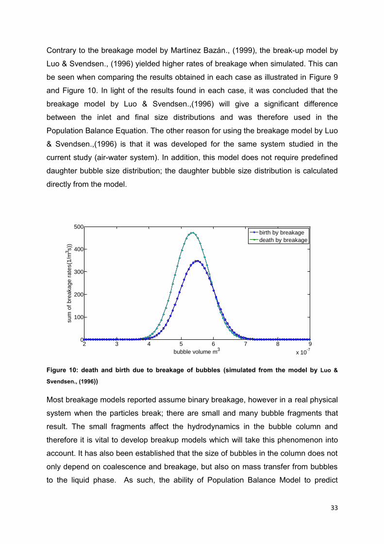
33

Contrary to the breakage model by Martínez Bazán., (1999), the break-up model by

Luo & Svendsen., (1996) yielded higher rates of breakage when simulated. This can

be seen when comparing the results obtained in each case as illustrated in Figure 9

and Figure 10. In light of the results found in each case, it was concluded that the

breakage model by Luo & Svendsen.,(1996) will give a significant difference

between the inlet and final size distributions and was therefore used in the

Population Balance Equation. The other reason for using the breakage model by Luo

& Svendsen.,(1996) is that it was developed for the same system studied in the

current study (air-water system). In addition, this model does not require predefined

daughter bubble size distribution; the daughter bubble size distribution is calculated

directly from the model.

Figure 10: death and birth due to breakage of bubbles (simulated from the model by Luo &

Svendsen., (1996))

Most breakage models reported assume binary breakage, however in a real physical

system when the particles break; there are small and many bubble fragments that

result. The small fragments affect the hydrodynamics in the bubble column and

therefore it is vital to develop breakup models which will take this phenomenon into

account. It has also been established that the size of bubbles in the column does not

only depend on coalescence and breakage, but also on mass transfer from bubbles

to the liquid phase. As such, the ability of Population Balance Model to predict

2 3 4 5 6 7 8 9

x 10-7

0

100

200

300

400

500

bubble volume m3

su

m o

f bre

aka

ge r

ate

s(1

/m3s))

birth by breakage

death by breakage

34

bubble size distribution can be combined with CFD to predict the influence of bubble

size in the flow field. On the mass transfer from bubbles to the liquid phase, CFD can

be used to predict this phenomenon and as a result the influence of mass transfer on

bubble size can be accounted for when PBM is incorporated into CFD.

2.3. Incorporating Population Balance into CFD

Over the past two decades bubble column reactors have found a wide application in

industries such as mining, food, petroleum, chemical and pharmaceutical (Luo &

Svendsen, 1996).This is due to their high rates of heat and mass transfer, ease of

operation, no moving parts and easy construction. The work done in modelling

hydrodynamics in these reactors includes experimental and modelling work. In the

past years only CFD was used in modelling the hydrodynamics in these reactors,

however some improvements were done by incorporating Population Balance into

CFD to include bubble size distribution.

Sokolichin & Eigenberger (1994) used one bubble size class to model drag force

term which is one of the key closures in the Euler-Euler framework. Bubble breakup

and coalescence were not considered and the mass exchange between the liquid

and gas phase was not considered as well. The use of constant bubble size in the

churn-turbulent flow regime is not a justified choice as bubble size distribution is wide

due to strong bubble-eddy collision and bubble-bubble interaction.

In view of the importance of bubble size distribution in the performance of bubble

column reactors, Shimizu et al. (2000) developed a simulation model based on gas

hold-up and gas-liquid mass transfer. The column was compartmentalised, and the

movement of the bubbles from one compartment to another was described. Gas

hold-up and interfacial area were calculated from bubble size distribution which is

predicted from the Population Balance Equation. In the prediction of mass transfer

coefficient the penetration theory which is dependent on bubble rise velocity was

used. The bubble rise velocity used is by Clift et.al. (1978) and the results could be

accurate if the bubble rise velocity is calculated from the microscopic force balance.

Their findings indicate that the evaluation of gas holdup and volumetric mass transfer

rates depends primarily on breakup and coalescence phenomena.

35

Krishna et al. (2000) developed a model for predicting scale dependence of bubble

column reactors operating in the churn-turbulent flow regime. In their work, the

bubble column reactor was considered to be made up of small and big bubbles and

all the phases were described in the Eulerian framework. The interaction between

bubbles was ignored and this is not a justified assumption in the churn-turbulent

regime where there is a strong bubble-bubble interaction and a wide bubble size

distribution. Their findings indicate that there is a good agreement between

experimental and simulated results for gas hold-up and liquid velocity. However

these results can be improved by implementing Population Balance Model to

account for bubble-bubble interactions.

Van Baten & Krishna (2011) improved the work by Krishna et al. (2000) in that they

followed exactly the same modelling approach but for bubble column reactors

operating at an elevated pressure. Although this work was an improvement from the

previous work, it still has some limitations in that it does not consider the bubble size

evolution and its influence in the flow field.

Olmos et al. (2001) combined PMB with Euler-Euler CFD representation to

investigate the operation of a cylindrical bubble column. This was done by using

Multiple Size Group (MUSIG) model implemented in CFX.4.3 commercial software.

The MUSIG is a model based on the two-fluid model and the Population Balance

approach. It was found that the hydrodynamic variables such as axial liquid velocity

and local gas hold-up are in good agreement with the experimental data. However,

when the flow is no longer homogenous, the predicted local Gas hold up was found

to give unreliable results. The results of the predicted bubble size distribution were

compared with the experimental results from the photographic technique and a good

agreement was found. The limitation in the model developed is that when the flow

transition begins, the predicted hydrodynamic variables no longer show a good

agreement with experimental data.

Chen et al. (2005) implemented Population Balance Equation into CFD Euler-Euler

representation to determine how well time averaged liquid axial velocity, kinetic

energy profiles and gas hold-up profiles can be predicted. It was found that a good

agreement between experimental and modelling work was found in terms of liquid

axial velocity and kinetic energy profiles, however in terms of gas hold-up no realistic

36

results were found. This could be explained by the fact that they used 2-D

axisymmetric simulation which does not capture the dynamic features of the flow

field like the 3-D simulations do.

On the other study, Wang et al. (2006) developed a coupled CFD-PBM model to use

the ability of CFD to calculate the entire flow field and that of PBM to calculate

bubble size distribution. In their work, the Population Balance was not implemented

into CFD by using the multiple-size group (MUSIG) as it was done in the previous

works. The MUSIG model is in the commercial CFD package, CFX and its breakup

and coalescence closures cannot be used over a wide range of operating conditions.

In their work, a full Population Balance Model with detailed coalescence and breakup

closure was implanted into Euler-Euler CFD representation. A good agreement was

found to experimental data in terms of gas hold-up profiles, liquid velocity and bubble

size distribution. It was also concluded that breakup and coalescence closures are

important in reliably predicting bubble size evolution in both heterogeneous and

homogeneous flow regimes. However, this conclusion contradicts with the work of

Chen et al. (2005) who concluded that the choice of break up and coalescence

closures does not have impact on the simulated results.

Wang et al. (2005) used the notion that bubble size distribution plays an important

role in the flow regime transition to develop a theoretical model based on PBM. The

bubble size distribution is effectively predicted from PBM, and from the bubble size

distribution flow regime transition can be predicted thereof. In their work, the two-fluid

model was combined with PBM and in this case all the bubble sizes were assumed

to have the same rise velocity. This assumption is justified in the homogenous flow

regime, but cannot be applied in the heterogeneous flow regime where there is

strong bubble-bubble interaction and bubble-eddy interaction. The findings in their

study indicate that bubble size distribution becomes wider with the increase of gas

hold-up. It was found out that in the heterogeneous flow regime, bubble size

distribution approaches equilibrium within a short period of time due to intensive

nature of break-up and coalescence at this flow regime.

Ekambara & Dhotre., (2007) combined PBM and CFD approach for simulating the

flow in an oscillatory baffled column. In coupling PBM with CFD, the Eulerian-

Eulerian two-fluid model was used. Break up and coalescence were considered in

37

simulating the hydrodynamics. The MUSIG model was used in determining the

temporal and geometrical changes of the gas bubbles .Their findings indicate that

the predicted hydrodynamics variables such as liquid velocity, local gas hold-up

showed good agreement to the experimental data.

Bhole et al. (2008) developed a combined CFD-PBM model in the Eulerian

framework for the simulation of axisymmetric steady state flows in bubble column

reactors. They calculated bubble size evolution from Population Balance Equation

and its influence in the flow field was calculated from CFD. In their work, the

assumption of identical velocities for bubbles of all sizes which was used in previous

work was eliminated by considering the simplified gas momentum equation. Thus in

this case the bubbles of different sizes were taken to move at different velocities and

the momentum balance for each size was solved. The simplified gas momentum

equation is called an algebraic slip model and since it’s an algebraic model, it solves

for the gas velocity in one step. They found that with CFD-PBM approach there is a

good agreement between numerical and experimental results for gas hold-up, axial

liquid velocity and kinetic energy in bubble column reactors. The limitation in this

study is that the full momentum equation for the gas phase is not solved since they

looked at the steady state simulation. In the cases where flow around individual

bubbles at fine grid and time step is needed the algebraic slip model is not

applicable.

Although there has been an improvement in the modelling of bubble columns by

incorporating Population Balance into CFD as intimated, there are some challenges

that still remain and those include the correct understanding of the physics in

multiphase flow, generic models that can be applied over a wide range of operating

conditions and computational expense.

2.6. Experimental work on investigating the hydrodynamics in bubble

columns

On the experimental work for determination of gas hold-up, Wu et al. (2001) used

gamma ray computed tomography. The experiments were conducted over a range of

superficial velocities (2 cm/s to 60 cm/s), at different pressures (0.1-1.0 MPa) with 5

38

different spargers and columns of different diameters ranging from (0.19-0.44 m).

Their findings indicate that, gas hold-up profiles change significantly with gas

velocity. On the effect of pressure they reported that, as pressure increases, the

bubble size distribution becomes narrow and this results in flatter gas hold-up which

is ascribed to uniform distribution of small bubbles. The effect of column diameter on

gas hold-up was also investigated, but the findings did not agree well with the known

and reported fact that, at larger column diameters, the liquid recirculation increases

hence steeper hold-up profiles are expected.

The study on the independent determination of mass transfer coefficient and

interfacial area was undertaken by Bouaifi et al., (2001). The local Gas hold-up was

determined by an optical probe connected to an Optoelectronic type Y module linked

to a computer. Their findings indicate that, for all types of sparges used, gas hold-up

increases with increasing superficial gas velocity. The porous and membrane

spargers were found to result in gas hold-up values greater than those in a

perforated plate sparger. This can be attributed to bubble size, gas hold-up in a

system of small bubbles is bigger than that in big bubble system. In addition, bubble

size is dependent on the type of sparger used, hence different results are found for

different sparger types.

Jamialahmadi & Müuller-Steinhagen (1993) conducted experiments in two different

columns using air and water at ambient temperature and atmospheric pressure to

investigate the effect of superficial velocity in bubble size, terminal bubble rise

velocity and gas hold-up. They highlighted the need for reliable estimate of the

aforementioned hydrodynamic parameters as they are directly related to the transfer

coefficient and transfer area. In their experiments, they measured bubble size and

bubble rise velocity using a micro-processor controlled camera and video equipment

in a two dimensional column. In the other set of experiments, a three dimensional

column was used and gas hold-up was measured from bed expansion. In their

findings it was demonstrated that the bubble diameter and gas hold-up increased

with increasing superficial gas velocity. Correlations for mean diameter and gas hold-

up were derived.

39

On the experimental work, Degaleesan et al., (2001) used computer-automated

radioactive particle tracking technique to investigate turbulence and liquid circulation

in bubble columns. The time average liquid velocity for columns of different sizes at

different operating conditions was investigated. Their findings indicate that time

average liquid velocity changes as the superficial gas velocity changes from 2.4 cm/s

to 12 cm/s and that this might mean that there is a change of flow regime from

bubbly flow to churn-turbulent.

On the experimental determination of bubble size distribution and gas hold-up in

bubble columns, Lage & Esposito., (1999) measured bubble diameters for a bubble

column operating in a homogenous regime at different values of superficial gas

velocity. In their work, it was assumed that the bubbles rise unperturbed and as a

result a direct relationship between bubble rise velocity and residence time is

achieved. This resulted in bubble size distribution in the column being determined

from experimental data using the conservation form of the bubble size distribution

function. The findings of their study indicate that at homogenous flow regime, the

bubble size distribution does not vary significantly along the column. However, in

other the flow regimes a non-uniform size distribution is observed and as a result the

shape of the bubbles changes from sphericity to other shapes and their velocities

differ.

2.4. Summary of literature review

Although over the past years there have been some improvements in the modelling

of bubble columns by integrating PBM into CFD, the current models are

computationally expensive and require high performance computing hardware. The

development of a fast-solving model to mitigate the computational burden promises

to be a better modelling approach in simulating bubble columns and can lead to a

wider application of PBM-CFD models. In addition, it is necessary to develop generic

models that predict hydrodynamic variables for a wide range of operating conditions

as most of the current models are restricted to the conditions under which they were

developed.

From the aforementioned previous work on prediction of hydrodynamics in bubble

column reactors, it can be said that it is still difficult to obtain the prediction of

hydrodynamic parameters for a particular system geometry over a wide range of

40

conditions. For instance, some studies investigate only the influence of column

diameter on heat and mass transfer, whereas the hydrodynamics are influenced by

many factors such as particle size, fluid velocity, density and thermal conductivity. In

addition, in the context of heat transfer, most of the studies concerned time averaged

local heat transfer coefficient and this does not give more information on

instantaneous effect of bubble dynamics on heat transfer.

The studies based on CFD are limited to homogeneous regime as they consider only

one bubble size. However, as the flow transition begins there is a complex

interaction between the continuous and dispersed phase. It is therefore necessary to

integrate Population Balance into CFD modelling of bubble columns for a better

understanding of different flow regimes and bubble characteristics in bubble columns

design and optimization. For reliable design and scale-up of these reactors, the gap

in the literature needs to be filled by developing models that predict the heat transfer

coefficient under a wide range of conditions. Coupling Population Balance with

Computational Fluid Dynamics can improve the predicted heat and mass transfer

coefficients. This is because interfacial area is an important parameter in heat and

mass transfer coefficient calculations and including PBM to account for bubble size

evolution can result in a reliable predictor.

41

Chapter 3

3. Research objectives and key questions

The current study attempted to approximate accuracy by accepting the work of

others as benchmarks to validate the developed model against. The studies in the

previous years have shown that the incorporation of CFD into the Population

Balance framework results in the accurate prediction of hydrodynamics in bubble

columns. This is ascribed to the fact that the Population Balance Model has the

ability to calculate particle size distribution, and the impact of size distribution in the

flow field can be predicted from CFD. In addition, the incorporation of CFD into the

PBM framework allows for the decoupling of the intrinsic mass transfer coefficient

and the specific interfacial area which helps in investigating what the mass transfer

rate will be in the column. In spite of this major development in the modelling of

hydrodynamics in bubble columns, computational expense still remains one of the

major challenges. It is therefore vital to develop models that reduce the

computational expense, while maintaining the accuracy in the prediction of the

hydrodynamics of interest. In addition, there are many correlations reported for the

prediction of hydrodynamics variables such as, Sauter mean diameter, interfacial

area and gas hold-up. However, these correlations cannot predict the

aforementioned parameters over a wide range of operating conditions as most of

them are specific to the conditions under which they were derived, equipment type

and geometry. Thus, it still remains a challenge to develop generic models that are

computationally efficient and that also capture all the dynamic features of the

multiphase flow even for heterogeneous flow regimes. As such, it is the objective of

this study to develop a fundamental model that accurately predicts hydrodynamic

parameters over a range of Re numbers.

3.1. Research objectives

The current study aspired to meet the flowing objectives.

Overall aim of the study

42

Development of a fundamental model that accurately predicts hydrodynamic

parameters over a wide range of Re numbers

Measurable objectives of the study

Predict gas hold-up, interfacial area, mass transfer rate and Sauter mean

diameter.

To decouple the intrinsic mass transfer coefficient (kL) from the specific

interfacial area (a), and investigate what the mass transfer rate will be in the

column.

To employ the analogy between heat and mass transfer in the prediction of

heat transfer coefficient from mass transfer results.

To compare the predicted flow field with the published experimental data for

an air-water system. (That is to validate population balance with heat and

mass integration).

3.2. Hypothesis

The impact of bubble size distribution in the flow field can be reliably predicted by

integrating Bubble Cell Model into the Population Balance framework. Size

distribution is an important parameter for modelling hydrodynamics in multi-phase

reactors, as it affects mass transfer by changing the interfacial area.

3.3. Key questions

How is Bubble Cell Model going to be integrated into the Population balance

framework?

Are the changes in the intrinsic mass transfer coefficient (kL) greater than the

changes in the specific interfacial area?

Does the integration of BCM into the PBM framework yield the results that

mimic reality?

Does the determination of heat transfer coefficient from mass transfer results

yield accurate results?

43

Chapter 4

4. Model development

In multiphase modelling, there are several modelling techniques that are employed,

namely: Euler-Euler, Euler-Lagrange, Direct Numerical Simulation etc. The intimated

modelling techniques are fluid property simulations that solve momentum, mass and

energy balance problems and in the context of bubble columns, they all take bubble

size to be constant. A commonly applied assumption is that bubble size is constant.

However, bubble columns have special needs in that there are bubbles of different

sizes in which case the constant size assumption must be relaxed. Over the past

years there has been extensive work in incorporating PBM in CFD to model local

size distribution, and thus local mass transfer coefficient, local gas hold-up and local

interfacial area (Scott & Richardson, 1997).

A Population Balance Model has the ability to predict local interfacial area and the

two-fluid model is used in most studies to predict mass transfer coefficient(Olmos et

al., 2001), thus the incorporation of Population Balance Modelling into the Euler-

Euler approach makes it possible to determine the intrinsic mass transfer coefficient

and interfacial area separately .The separate prediction of these two parameters

allow for decoupling transfer mechanisms, and it can therefore be determined which

factor controls mass transfer (Bouaifi et al., 2001). The independent determination of

the intimated parameters is vital as it cannot be predicted what the mass transfer

rate will be when the bubbles rise through the column, since it is not known if the

changes in the intrinsic mass transfer coefficient will be greater than the changes in

the interfacial area. For this reason, it is important to decouple (kL) from (a), and

once that is done, it becomes possible to investigate this question. Therefore in

adopting this approach, the use of the volumetric mass transfer coefficient (kLa) in its

lumped form (intrinsic mass transfer coefficient multiplied with specific interfacial

area) can be obviated. The current work aimed at integrating Bubble Cell Model into

the Population Balance framework as the aforementioned modelling approaches

demand high computational time and memory requirement. In this section, a detailed

methodology on how the BCM was integrated into the PBM framework will be

presented. The low computational expense of BCM makes it suitable as a sub-model

44

in the macro-modelling of hydrodynamics in bubble columns making its integration

into the PBM framework feasible.

4.1.Bubble Cell Model

In its current development, a Bubble Cell Model is an algebraic model that predicts

the spatial velocity vector fields in the vicinity of a single bubble (Coetzee et al.,

2011). The extension of BCM to concentration and thermal gradients can therefore

prove vital in the modelling of bubble column reactors. In a similar approach to that

of velocity vector fields, in the context of concentration fields, BCM can be extended

to predict spatial concentration fields in the vicinity of a single bubble. In the

prediction of spatial concentration fields using BCM, Reynolds number is specified

and the full Navier-Stokes equations are solved in CFD. Upon solving the Navier-

Stokes equation, pressure, velocity, concentration and temperature fields can then

be determined. Since the current work focuses on the concentrations fields, only the

concentration gradients determination will be discussed in this section. Upon the

determination of concentrations fields and mass transfer coefficient thereof, heat

transfer coefficient is predicted from mass transfer results by employing the analogy

that exists between heat and mass transfer as illustrated in section (2.1.8).

The Navier-Stokes equations describe the motion of fluid substances and they are

derived from assuming that the fluid under study is a continuum i.e. the fluid element

is not moving at relativistic velocity (Batchelor,1967). The Equations (4.1) and (4.2)

represent the Navier-Stokes equations for an incompressible flow of Newtonian

fluids. The solution of the Navier-Stokes equations yields the data to be

approximated which can be velocity gradients, pressure gradients, heat and mass

transfer coefficients. In the current work, the data to be approximated constitute the

heat and mass transfer coefficients. The mass transfer coefficient is approximated

from BCM by specifying Reynolds and Sherwood numbers and the heat transfer

coefficient is approximated from mass transfer results by employing the analogy that

exists between heat and mass transfer.

(4.1)

45

(4.2)

The mass transfer coefficient was approximated by correlating Reynolds and

Sherwood numbers. The full Navier-Stokes equations are solved in CFD and that

yields the concentration profiles in the vicinity of a single bubble. The data from the

solution of the Navier-Stokes equations is used to predict mass transfer coefficient

by employing the film theory. The data from CFD for approximating the mass transfer

coefficient in the vicinity of a single bubble at the Reynolds (Re) is fitted with a

polynomial and this makes it possible to predict mass transfer coefficient at the new

Reynolds number (Re1). The Matlab function polyfit presented in Equation (4.3) finds

the coefficients of a polynomial of the degree of interest that fits the data .The

correlation of Reynolds and Sherwood numbers is done as follows:

3

(4.3)

In Equation (4.3), Re number used to generate data from CFD is correlated with

Sherwood number and this makes it possible to approximate Sherwood number from

any Reynolds number given and that is done as follows:

(4.4)

The Matlab function polyval presented in Equation (4.4) takes the input argument km

and returns a polynomial of the degree of interest evaluated at Re1. At the new

Reynolds number (Re1), Sherwood number is approximated as illustrated in

Equation (4.4) and mass transfer coefficient can be predicted thereof. This makes

BCM extremely fast in predicting hydrodynamic variables as opposed to the Euler-

Euler, Euler-LaGrange and Direct Numerical Simulation. The computational time of

the method proposed will be demonstrated in the sections to follow.

Convective

acceleration

Pressure

gradient Viscosity Other body

forces

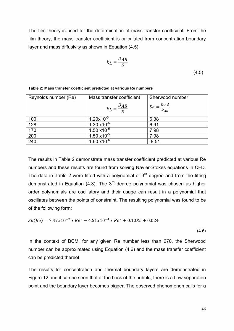
46

The film theory is used for the determination of mass transfer coefficient. From the

film theory, the mass transfer coefficient is calculated from concentration boundary

layer and mass diffusivity as shown in Equation (4.5).

(4.5)

Table 2: Mass transfer coefficient predicted at various Re numbers

Reynolds number (Re)

Mass transfer coefficient

Sherwood number

100 1.20x10-5 6.38 128 1.30 x10-5 6.91 170 1.50 x10-5 7.98 200 1.50 x10-5 7.98 240 1.60 x10-5 8.51

The results in Table 2 demonstrate mass transfer coefficient predicted at various Re

numbers and these results are found from solving Navier-Stokes equations in CFD.

The data in Table 2 were fitted with a polynomial of 3rd degree and from the fitting

demonstrated in Equation (4.3). The 3rd degree polynomial was chosen as higher

order polynomials are oscillatory and their usage can result in a polynomial that

oscillates between the points of constraint. The resulting polynomial was found to be

of the following form:

4 4 5 4

(4.6)

In the context of BCM, for any given Re number less than 270, the Sherwood

number can be approximated using Equation (4.6) and the mass transfer coefficient

can be predicted thereof.

The results for concentration and thermal boundary layers are demonstrated in

Figure 12 and it can be seen that at the back of the bubble, there is a flow separation

point and the boundary layer becomes bigger. The observed phenomenon calls for a

47

need to average the boundary layer as it is not uniform along the bubble surface.

The averaging is done as observed in Equation (4.7).

∫

(4.7)

Thus for an angle (θ) along the circumference of the bubble, the boundary layer can

be averaged as shown in Equation (4.7).

The Bubble Cell Model entails two stage fitting process. In the first stage, the spatial

concentration fields are approximated, and in the second stage, the stage one model

parameters are pre-correlated as a function of Reynolds number. In the first method,

as illustrated above, Reynolds number was correlated with Sherwood number and

an algebraic equation was derived. The derived equation expresses Sherwood

number as a function of Reynolds number. In the second method, Reynolds number

was correlated with the concentration boundary layer and the algebraic equation was

derived which expresses concentration boundary layer as a function of Reynolds

number. The mass transfer coefficient was predicted from the two methods and the

results were compared as depicted in Figure 11. When varying the Reynolds

number to predict mass transfer coefficient, the two methods show a close

agreement with an average relative difference of 0.8 %.

Figure 11: Mass transfer coefficient predicted from correlating Re with Sh and Re with δ

100 120 140 160 180 200 220 240 260 2805.5

6

6.5

7

7.5x 10

-5

Reynolds number

mass t

ransfe

r coeff

icie

nt

(m/s

)

Re correlated with Sh

Re correlated with

48

Table 3: Concentration boundary layer predicted at various Re numbers

Reynolds number (Re)

Mass transfer coefficient

Concentration boundary

layer (m)

100 1.20x10-5 3.70 x10-5 128 1.30 x10-5 3.20 x10-5 170 1.50 x10-5 2.80 x10-5 200 1.50 x10-5 2.70 x10-5 240 1.60 x10-5 2.60 x10-5

Upon fitting the data in Table 3 to derive a correlation that expresses concentration

boundary layer as a function of Reynolds number, the mathematical formulation as

illustrated in Equation (4.8) is found. The expression makes it possible to predict the

concentration boundary layer from Reynolds number as the input and upon

predicting the boundary layer, the mass transfer coefficient can be predicted using

the film theory as illustrated in Equation (4.5).

4 5 3 5 4 5

(4.8)

49

Figure 12: Concentration (δc) and thermal (δt) boundary layers

Since BCM is Reynolds number dependent, the bubble rise velocity for the

population of bubbles was calculated from force balance, and their Reynolds number

used to predict mass transfer coefficient. A schematic diagram on how BCM was

integrated into the PBM framework is shown in Figure 25.

4.1.1. Bubble rise velocity

Bubble rise velocity is one of the most important parameters that govern the

performance of a bubble column reactor. The hydrodynamic parameters such as

gas hold-up, mass transfer and interfacial area are influenced by the bubble rise

velocity; because bubble rise velocity dictates how much time a bubble spends in the

column.The rise velocity of bubbles is calculated from the macroscopic force balance

and can be expressed mathematically as illustrated in Equation (4.9).

(4.9)

Where the forces on the right hand side of the equation represent gravity, pressure

gradient, drag, lift and virtual mass. The closure correlations for the forces on the

right hand side are reported in the literature (Delnoij et al., 1997) and they are as

shown in Equation (4.10) through (4.14).

50

(4.10)

(4.11)

| | (4.12)

(4.13)

(

) (4.14)

The bubble rise velocity at each time step in the column is calculated as presented

in Equation (4.15).

(4.15)

Where u (j) is the velocity of a bubble at its current position and u (j-1) is its velocity

from previous position, the time step Δt, and its acceleration

at the current

position. However in the current work, the bubble terminal velocity is considered and

it is calculated from assuming a net force of zero from the forces mentioned above

and it is calculated as follows:

√

(4.16)

The bubble terminal velocity calculated from force balance in Equation (4.16) was

validated against the bubble rise velocity from the other forms of force balances

reported in the literature. The results in Figure 13 show that the bubble rise velocity

calculated from force balance in the model are in good agreement to the bubble rise

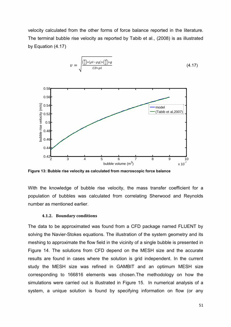
51

velocity calculated from the other forms of force balance reported in the literature.

The terminal bubble rise velocity as reported by Tabib et al., (2008) is as illustrated

by Equation (4.17)

√(

) (

)

(4.17)

Figure 13: Bubble rise velocity as calculated from macroscopic force balance

With the knowledge of bubble rise velocity, the mass transfer coefficient for a

population of bubbles was calculated from correlating Sherwood and Reynolds

number as mentioned earlier.

4.1.2. Boundary conditions

The data to be approximated was found from a CFD package named FLUENT by

solving the Navier-Stokes equations. The illustration of the system geometry and its

meshing to approximate the flow field in the vicinity of a single bubble is presented in

Figure 14. The solutions from CFD depend on the MESH size and the accurate

results are found in cases where the solution is grid independent. In the current

study the MESH size was refined in GAMBIT and an optimum MESH size

corresponding to 166816 elements was chosen.The methodology on how the

simulations were carried out is illustrated in Figure 15. In numerical analysis of a

system, a unique solution is found by specifying information on flow (or any

2 3 4 5 6 7 8 9 10

x 10-7

0.42

0.44

0.46

0.48

0.5

0.52

0.54

0.56

0.58

bubble volume (m3)

bubble

ris

e v

elo

city (

m/s

)

model

(Tabib et al,2007)

52

dependent) variables at the domain boundaries. In the current work the boundary

conditions are velocity inlet, outflow, symmetry and axis, wall and bubble.

Figure 14: Mesh generation for the system under study

Velocity Inlet

In the incompressible flow, one of the system boundary conditions is the velocity

inlet. The inlet velocities used were in the range 0.0893 to 0.271 m/s and that

translates to Re number in the range 100 to 270.

Outflow

In the case of outflow, pressure and velocity need not to be specified as the data at

the exit plane is extrapolated from the interior (Fluent, 2009). The mass balance

correction is applied in the outflow boundary.

Symmetry and axis

In the context of symmetry boundary, the requirement is that the flow and geometry

be symmetric. The importance of this boundary is that it reduces computational effort

for the problem under study (Fluent, 2009).

Wall

For the wall, the zero-shear-stress (free-slip) condition has been adopted at the

rectangular wall. This choice was based on the notion that the walls do not represent

the actual walls of a bubble column, but are only used to create a computational

domain where the fluid around the bubble is bound (Fluent, 2009).

53

Bubble

The bubbles in the bubble column do not exert a shear stress to the continuous

phase and in light of that a zero-shear-stress was adopted.

Post-processing

Solver

Pre-processing

4.data to be approximated. E.g. concentration boundary layer, temperature boundary

layer. etc

3. run the model to execute the commands and solve the Navier-

Stokes equation

2.Inputs: Re and Sc

1. create geometry and generate mesh

Re,Sc

Figure 15: The CFD methodology for approximating mass transfer coefficient

4.2. Numerical estimation of heat and mass transfer coefficients

Heat and mass transfer coefficients are the important design parameters in bubble

columns and the accurate prediction of these parameters is crucial. Mass transfer

refers to the relative motion of species from one phase, stream or component to

another due to concentration gradients. In the current study, mass transfer is from

the gas bubbles to the continuous phase and the methodology on how total mass

transfer was calculated will be outlined.

54

The mass balance on the solution surrounding the bubbles under the assumption of

perfect mixing and the volume and volumetric flow-rate being time constants, can be

expressed as shown in Equation (4.18)

(4.18)

Where rA is the mass transfer rate and can be expressed as shown in Equation

(4.19).

(4.19)

Substituting rA into Equation (4.18), the following form is found:

(4.20)

In the current study, steady state is considered, and the term on the left side of

Equation (4.20) becomes zero, and the concentration of air can be expressed as

shown In Equation (4.21).

(4.21)

Where ap is the gas-liquid interfacial area. cA0 is the gas initial concentration in the

column, cAs is the gas concentration at the gas-liquid interface and cAb is the gas

concentration in the bulk liquid. The interface gas concentration is calculated from

Henry’s law because at the interphase equilibrium is achieved. The data on the

Henry’s constant of Air is not readily available for specific operating conditions. Since

55

Air comprises Oxygen and Nitrogen, the concentrations of the two were calculated

and from their results air concentration was calculated as presented in Equation

(4.22).

(4.22)

Where P is total pressure, Y02 is the mole fraction of Oxygen in the gas phase, XO2 is

mole fraction of Oxygen in the liquid phase, ɣO2 is the activity coefficient and H is the

Henry’s constant.

Thus for an ideal solution ɣ*O2 =1, and Equation (4.22) reduces to the form

expressed in Equation (4.23).

(4.23)

(4.24)

The units of the solubility are g/L and to convert this to concentration of oxygen (C02)

in water, the solubility calculated in Equation (4.24) is divided by the Molecular

weight of oxygen. The similar methodology is followed for the concentration of

Nitrogen, and upon getting the concentrations of Oxygen and Nitrogen in the liquid

phase; the concentration of air is calculated as shown in Equation (4.25).

∑

(4.25)

56

Where xj is the mole fraction of compound j in water and C is the concentration. The

other parameter that needs to be known for the determination of total mass transfer

rate is the mass transfer coefficient. In the current study, the intrinsic mass transfer

coefficient is predicted from BCM by employing the two film theory as illustrated in

section (4.5)

4.2.1. Heat and mass transfer analogy

An analogy exists in the mathematical descriptions of both heat and mass transfer

and in the conditions where this analogy holds, heat transfer can be predicted from

mass transfer results, thus obviating a need to perform heat transfer coefficient

determination which is normally a difficult task to achieve experimentally. The

analogy can further be seen in the predicted thermal and concentration boundary

layers which follow the same trend as depicted in Figure 12. The boundary layer

results as shown in Figure 12 are in agreement with the reported work (Khan & Pop,

2010) on concentration and thermal boundary layer, which states that the thermal

boundary layer is larger in thickness as compared to the concentration boundary

layer. In the current study, this analogy was tested and found to hold as illustrated in

Figure 18. The heat transfer coefficient was predicted from CFD and the results

were compared with the heat transfer coefficient predicted from mass transfer

results. The findings indicate that heat transfer coefficient predicted from both cases

show a similar trend and the average difference between the two methods is 7.63 %.

Upon averaging the boundary layers in the vicinity of a single bubble as illustrated in

Equation (4.7), the thermal and concentration boundary layers are as depicted in

Figure 16 and Figure 17. The results for the two boundary layers show a similar

trend and it can be concluded that heat and mass transfer follow the same velocity

profile and this is a condition to be met for the analogy to be applicable. The

graphical representation in Figure 12 shows the temperature and concentration

profiles around a spherical bubble, and when averaging the profiles, the numerical

results of the boundary layers can be observed in Figure 16 and Figure 17. The

findings are in agreement with the general notion that the thermal boundary layer is

greater in magnitude compared to the concentration boundary layer.

57

Figure 16: Concentration boundary layer in the vicinity of a single bubble at various Reynolds number

Figure 17: Thermal boundary layer in the vicinity of a single bubble at various Reynolds number

The determination of heat transfer coefficient from mass transfer coefficient was

performed as demonstrated in section (2.1.8). The heat transfer coefficient results

were validated by comparing the predicted Nusselt number with the Nusselt number

calculated from empirical correlations.

100 120 140 160 180 200 220 240 260 2802.4

2.6

2.8

3

3.2

3.4

3.6

3.8

4x 10

-5

Re

c

Concentration boundary layer at various Re numbers

100 120 140 160 180 200 220 240 260 2806.5

7

7.5

8

8.5

9

9.5

10

10.5

11x 10

-5

Re

t (

m)

Thermal boundary layer at various Re numbers

58

Figure 18: heat transfer coefficient prediction by analogy and CDF determination

4.3. Population Balance Model

The Population Balance Equation was first presented by Hulburt & Katz,. (1964) and

is now used in many applications including crystallization, flotation, gas-liquid

dispersion and liquid-liquid extraction. The Population Balance for any system is a

mathematical framework used to determine property distributions of discrete

properties such as particles, oil droplets and gas bubbles (Ramkrishna & Mahoney,

2002; Yeoh & Tu, 2004). The population in the system is described by the density of

the extensive variables such as number, volume or mass of particles (Ramkrishna &

Mahoney, 2002; Yeoh & Tu, 2004). The focus of PBM is on the distribution of the

particle population and its impact in the system behaviour. In the system the particles

either form or disappear and thus the number of particles changes with position and

time in the reactor and this is taken into account by a Population Balance. In the

context of gas bubbles, the change in the number of particles is due to either break

up or coalescence. In the break up process, the new smaller particles are formed

from the breakage of the parent particles. On other hand, in coalescence, particles

collide and merge to form particles of bigger size.

The general Population Balance Equation is expressed mathematically as follows:

100 120 140 160 180 200 220 240 260 2805000

5500

6000

6500

7000

7500

8000

8500

9000

Reynolds number

He

at

tra

nsfe

r co

eff

icie

nt

(W/m

2.K

)

hc predicted from CFD

hc predicted from heat and mass transfer analogy

59

( )

(4.26)

In Equation (4.26), α is the chosen set of properties (e.g. size, position, activity etc.).

The factor is the rate at which the property (α) changes with time, thus the

second term on the left hand side represents the change at which properties of the

population change spontaneously with time. The terms on the right hand side

represent the rate at which bubbles are born and die from the population due to

break up and coalescence. The first term on the right hand side represents the birth

of particles due to break up or coalescence, while the second term represents death

of particles due to the same processes.

Since (α) is a set of properties as indicated, in the present case a more appropriate

choice to a bubble column was made by assuming (α) to be a set of spatial co-

ordinates and bubble diameter. Therefore, the internal co-ordinates considered are

the bubble number density probability distribution, bubble diameter and the spatial

coordinates. The first term in the left hand side of the equation represents the

change in ψ with respect to time. In the context of a Population Balance Equation, ψ

is a multivariable distribution function, where the variables of the distribution are the

properties α.

From the general form of a Population Balance Equation as presented in Equation

(4.26), the form adopted in the current study is as follows:

(

)

∫

∫

(

)∫

∫

(4.27)

60

In the form of the Population Balance Equation in (4.27); the first term on the right

hand side represents the change in bubble diameter due to mass transfer, the

second and third terms represent the birth and death of bubbles due to break up.

The last two terms are the representation of birth and death due to coalescence. The

steady state population balance was adopted, and thus the first term in the left hand

side becomes zero and the variation of the properties is considered in one

dimensional space (axial). This term can be expanded as follows:

(

)

(4.28)

When adapting the steady state context, the bubbles are assumed to rise at terminal

velocity and as a result the variation of bubble velocity with respect to column height

becomes zero, thus the first term in Equation (4.28) becomes zero. Since all the

bubbles attain terminal velocity, the collision is linked to bubble size as only the mass

of the bubble will affect the velocity in this case. The bubble terminal velocity is

calculated from force balance as illustrated in Equation (4.16). It was stated

previously from the work of Bhole et al., (2008) that the use of steady state

simulation has limitations in that the full momentum equations for the gas phase is

not solved. However in the current study, with fully knowledge of this limitation, a

steady state Population Balance Equation was used. This was done because the

current study aimed at integrating BCM into the PBM framework to predict the

hydrodynamic parameters over a wide range of Re numbers. Upon a successful

integration of BCM into the PBM framework for mild conditions, the unsteady state

simulations can then be incorporated to enhance the accuracy of the predicted

hydrodynamic parameters.

The right hand side of the Population Balance Equation (4.27) represents death (D)

and birth (B) of particles due to break up and coalescence, and upon solving the

PBE, the knowledge of the functions that describe break up and coalescence is

essential. There are several models for both break up and coalescence reported in

the literature.

61

4.3.1. Coalescence model

Coalescence is the process whereby particles collide and merge to form new

particles. It is examined in terms of particles collision and the likelihood that their

collision will result in coalescence. Several coalescence models have been reported

in the literature. The coalescence model of Prince & Blanch., (1990) is as shown in

Equation (2.9).

(4.29)

Where Ωc is the coalescence rate (m-3s-1), and θijT

,θijB

,θijLS are; turbulent collision rate,

buoyancy driven collision rate and laminar shear collision rate respectively.

4.3.1.1. The turbulent collision rate

In the turbulent collision type, the bubbles collide due to the fluctuating nature of the

liquid phase velocity and the collision frequency that results from the turbulent

motion of the liquid phase is as expressed as presented Equation (4.30).

(ῡ ῡ )

(4.30)

Where fi and fj are the number densities for the bubbles of size groups i and j. Sij is

the cross-sectional area for collision of the bubbles, while ῡtj and ῡti are the average

fluctuating velocities for the bubbles of sizes j and i respectively. Each of the

aforementioned parameters can be expressed mathematically as shown in Equation

(4.31) and (4.32).

4

(4.31)

Where rbi and rbj are the radii of the bubbles of sizes i and j respectively. The average

turbulent fluctuating velocities can be expressed as a function of bubble size as

follows:

62

ῡ 4

(4.32)

4.3.1.2. Buoyancy-determined collision rate

In the buoyancy collision type, the bubbles collide as a result of their different rise

velocities and the frequency of collisions that results from difference rise velocities is

expressed as follows:

𝑈 𝑈

(4.33)

According to Clift et al., (1978), the bubble rise velocity Uri can be expressed as

illustrated in Equation (4.34)

𝑈 ( 4𝜎

5 5 )

(4.34)

4.3.1.3. Laminar shear collision rate

In the laminar shear collision type, the collision of particles results from the gross

circulation pattern that is encountered in bubbles column operating at high gas flow

rates and is expressed mathematically as presented in Equation (4.35).

4

3

( ῡ

)

(4.35)

4.3.2. Break up model

Bubble break up happens when the bubble cannot withstand the internal forces or

the external forces created by the surrounding fluid. Bubble break up can also be

explained to occur when the bubbles collide with the turbulent eddies. The eddies

that lead to bubble break up are those that have the length scale equal to or less

than the bubble size (Lehr, Millies & Mewes, 2002; Luo & Svendsen, 1996; Prince

& Blanch, 1990). Several breakup models have been reported in the literature and

the breakup model by (Luo & Svendsen, 1996) is as shown (4.36).

63

(

)

∫

𝜎

(

)

(4.36)

Where ΩB(vi: vfBV) is the rate of breakup of a parent bubble with volume v to a

daughter bubble of size vfVB.

The other break up rate by Martìnez Bazán., (1999) is as presented in Equation

(4.37).

√

(4.37)

Where the constants β=8.2 and Kg =0.25 and were found experimentally by Martìnez Bazán (1999)

The breakage function by Martìnez Bazán., (1999) only calculates the probability

that a parent bubble will break to yield some daughter bubbles, it does not calculate

the size distribution of daughter bubbles, and hence a redistribution function is

needed (Patruno et al., 2009). The redistribution function is shown in Equation

(2.36). The total breakage rate from the two models is demonstrated in section

(2.2.4) and the observations indicate that the model by Luo & Svendsen (1996) show

higher breakage rates as compared to the model by Martìnez Bazán (1999). The

model by Luo & Svendsen (1996) was therefore used as it would yield a wider size

distribution compared to the other model which yields low breakage rates.

As intimated, the right hand side of Equation (4.26) represents the death and birth of

particles due to break-up and coalescence respectively. The total events that lead to

birth of particles (B) due to break-up and coalescence can be expanded as shown in

Equation (4.38).

64

∫

(

)∫

(4.38)

The total events that lead to death of particles (D) as expressed in the Population

Balance Equation can be expanded as presented in Equation (4.39).

∫

∫

(4.39)

The expressions B and D are birth and death rates terms in the Population Balance

Equation. When solving the PBE, the knowledge of these two terms is crucial.

4.3.3. A solution to the Population Balance Equation

In solving the Population Balance Equation, the initial and boundary conditions need

to be specified. The form of Population Balance Equation adopted in the current

study has a gas expansion term due density changes and mass transfer. The gas

density was assumed to be constant and the mass transfer rate was calculated from

BCM and this explains how BCM was integrated into the Population Balance

framework. The Population Balance Equation was solved by employing the discrete

method. In the discrete method, the particle size distribution is represented as a set

of discrete size classes as illustrated in Figure 19.

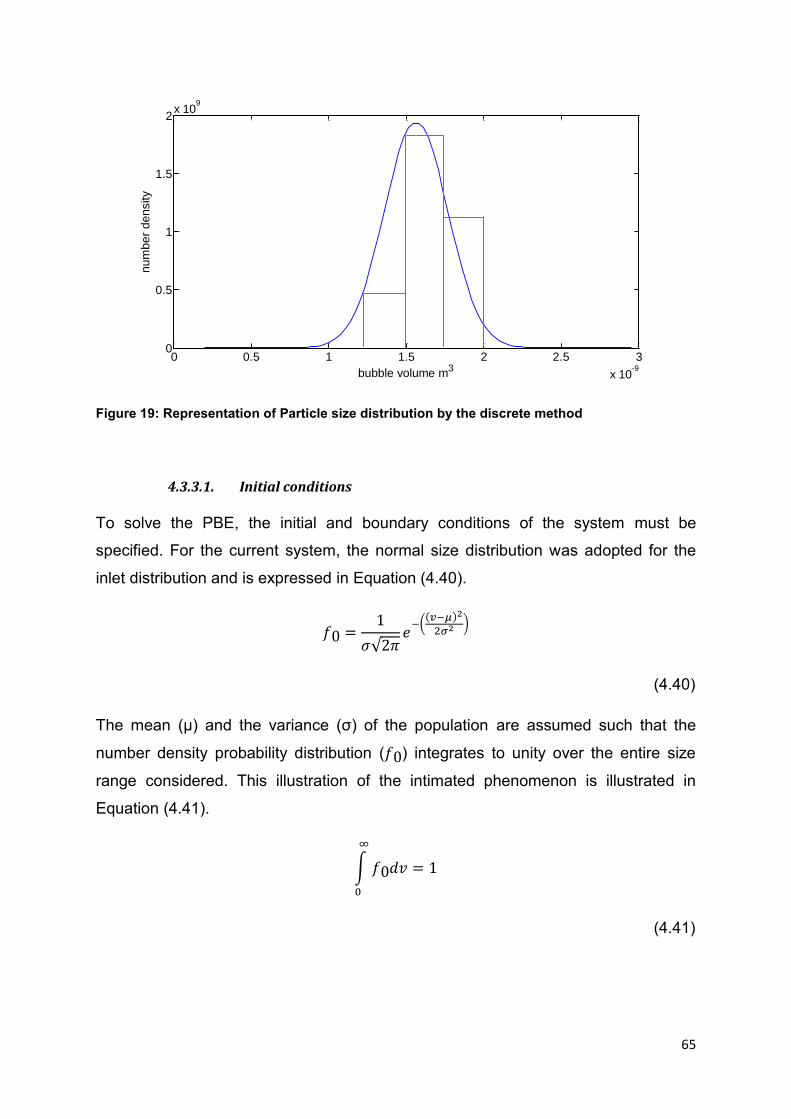
65

Figure 19: Representation of Particle size distribution by the discrete method

4.3.3.1. Initial conditions

To solve the PBE, the initial and boundary conditions of the system must be

specified. For the current system, the normal size distribution was adopted for the

inlet distribution and is expressed in Equation (4.40).

𝜎√ (

)

(4.40)

The mean (μ) and the variance (σ) of the population are assumed such that the

number density probability distribution ( ) integrates to unity over the entire size

range considered. This illustration of the intimated phenomenon is illustrated in

Equation (4.41).

∫

(4.41)

0 0.5 1 1.5 2 2.5 3

x 10-9

0

0.5

1

1.5

2x 10

9

bubble volume m3

num

ber

density

66

4.3.3.2. Boundary conditions

The boundary conditions were set for size distribution and this is shown in Equation

(4.42) through (4.44).

(4.42)

(4.43)

(4.44)

Where f is the final number density probability distribution. The latter boundary

condition states that there are no bubbles of zero size

4.3.3.3. A compartment model

The bubble size distribution is not constant in the column due to bubble-bubble

interaction and eddy-bubble interaction, and it is therefore vital to compartmentalise

the column and predict size distribution at each column compartment. In doing so, it

can be investigated and confirmed as to whether bubble size distribution varies

along the column. In the present work, the column was compartmentalised to

investigate the aforementioned phenomenon and also to predict the other

hydrodynamic parameters at each compartment. The column was

compartmentalized as depicted in Figure 20 and the hydrodynamics variables were

predicted in each column compartment. The choice of initial conditions for each

compartment is as given in Equation (4.45).

1st compartment

√ (

)

(4.45)

The exit bubble size distribution from the first compartment is taken as the inlet size

distribution to the second compartment. The same methodology is applied in other

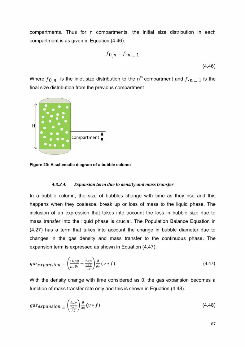
67

compartments. Thus for n compartments, the initial size distribution in each

compartment is as given in Equation (4.46).

(4.46)

Where is the inlet size distribution to the nth compartment and is the

final size distribution from the previous compartment.

H

compartment

Figure 20: A schematic diagram of a bubble column

4.3.3.4. Expansion term due to density and mass transfer

In a bubble column, the size of bubbles change with time as they rise and this

happens when they coalesce, break up or loss of mass to the liquid phase. The

inclusion of an expression that takes into account the loss in bubble size due to

mass transfer into the liquid phase is crucial. The Population Balance Equation in

(4.27) has a term that takes into account the change in bubble diameter due to

changes in the gas density and mass transfer to the continuous phase. The

expansion term is expressed as shown in Equation (4.47).

(

)

) (4.47)

With the density change with time considered as 0, the gas expansion becomes a

function of mass transfer rate only and this is shown in Equation (4.48).

(

)

) (4.48)

68

In Equation (4.48), ṅ is the molar flux, ap interfacial area, αg is gas hold-up and μg is

viscosity of the gas phase. The molar flux is calculated as shown in Equation (4.49).

∬

(4.49)

The gas-liquid interfacial area is expressed as presented in Equation (4.50).

∫

(4.50)

The mass transfer coefficient (kL(u,d)) is calculated from correlating the two

dimensionless numbers Re and Sh. The Bubble Cell Model predicts the intrinsic

mass transfer coefficient in the vicinity of a single bubble from Re number as the

input to the model. However, in the bubble column, there are multiple bubbles of

different sizes, hence different Re numbers. It is therefore vital to correlate Re and

Sh numbers in order to predict the mass transfer coefficient for bubbles of different

Re numbers. Having correlated the two, the local mass transfer coefficient for a

population of bubbles in the column can then be calculated using the information

from BCM. The methodology is as shown in Equation (4.51).

3

(4.51)

Where polyfit is a built-in-function in Matlab that is used to fit data using polynomials

and in this case it returns some coefficients for the polynomial of third degree. The

polynomial is of the form shown in Equation (4.52).

3 3

(4.52)

At the new Re numbers for a multiple bubbles in the column, the new Sherwood

number is calculated from the Reynolds number using the polynomial described in

Equation (4.52). With the knowledge of the form of the polynomial that describes the

69

data from BCM, the Reynolds number for the current case can then be used to

calculate the Sherwood number, hence the mass transfer coefficient. The following

procedure is used to calculate the new Sherwood number.

(4.53)

Where Sh,new is the new Sherwood number calculated from the new Reynolds

number for multiple bubbles in the column. The polyval function used is a built-in-

function in Matlab and it returns the value of the polynomial of degree 3 (in this

present case) which is evaluated at the new Reynolds number (Re1). With the

knowledge of Sherwood number as shown is Equation (4.53), the mass transfer

coefficient is calculated as shown in Equation (4.54).

(4.54)

The results in Figure 21 are for a flow over a single bubble and they show mass

transfer coefficient as a function of Reynolds number as predicted from CFD. The

findings indicate that mass transfer coefficient increases with increasing Re number

due to increased rates of mixing and the advection terms dominating in the Navier

Stokes equation. In a case where there are multiple bubbles in the column,

polynomial interpolation is employed by correlating Sherwood number with Reynolds

number and calculating the mass transfer coefficient for a population of bubbles as

illustrated in Equation (4.54). The results of mass transfer coefficient for a population

of bubbles are as shown in Figure 22. The similar trend of mass transfer coefficient

increasing upon an increase in Re number is observed.

70

Figure 21: mass transfer coefficients results from BCM

Figure 22: Mass transfer coefficient for a population of bubbles

4.4. Numerical estimation of overall heat and mass transfer coefficients

The Bubble Cell Model predicts the heat and mass transfer coefficients in the vicinity

of a single bubble. In the bubble column where there is multiplicity of bubbles of

different sizes, there is a need to predict heat and mass transfer coefficient for a

population of bubbles and the overall heat and mass transfer coefficients thereof.

The overall heat and mass transfer coefficients were predicted from the average

properties as illustrated in Equation (4.55) and (4.56).

100 120 140 160 180 200 220 240 260 2805

5.5

6

6.5

7

7.5x 10

-5

Reynolds number

Mass t

ransfe

r coeff

icie

nt

(m/s

)

1 2 3 4 5 6 7 8 9

x 10-10

5

5.5

6

6.5

7

7.5x 10

-5

Bubble volume (m3)

Mass t

ransfe

r coeff

icie

nt

(m/s

)

71

∫

(4.55)

Where kL,tot is the overall mass transfer coefficient calculated from the total number

of bubbles in the column. Multiple population balance equations were solved by

adopting the compartment approach, and as a result the overall mass transfer

coefficient was predicted at the discrete column compartments chosen. Upon

predicting the overall mass transfer coefficient, the analogy between heat and mass

transfer as discussed in section 4.2.1 was used to predict heat transfer coefficient.

The overall heat transfer coefficient for a population of bubble in the column was

predicted as follows:

∫

(4.56)

Upon determining the overall heat and mass transfer coefficients, the total heat and

mass transfer rates in the column can be predicted.

4.5.Numerical stability and convergence

In numerical methods, numerical stability and convergence are crucial for the

accuracy of the parameters estimated. When estimating the parameters on grid

points, it is of paramount importance to find optimum grid points where the solution is

grid independent. The stability of the solution is achieved by the use of a fine mesh

resolution. The grid independence was achieved by predicting the parameters at

different grid points and changing the grid points until the predicted parameter does

no longer change with grid size.

4.5.1. Size range and meshing

As specified in the above section, the inlet distribution and boundary conditions need

to be specified. The initial bubble size used translates to the size of bubbles that are

sparged into the column and their size depends on the diameter of the holes of the

sparger. The choice of the initial bubble size in the present case was arbitrary as

different spargers can have varying hole diameters. Upon choosing the initial bubble

72

size, a high resolution mesh was adopted to preserve the accuracy of the model.

The criterion used in determining the optimum grids points was an iterative one,

where the optimum grid points were found in a case where the solution of the

predicted parameter converged. This phenomenon can be observed in Figure 23

where the predicted Nusselt number was found to be independent of grid size

starting from 100 grid points. In the solution of the Population Balance Equation,

bubble size distribution and some other hydrodynamic parameters are predicted at

all the grid points considered.

Figure 23: The grid dependence of the predicted Nusselt number

4.6. Model Consistency checks

A model consistency check was done on the Population Balance to ensure that the

model is consistent in its prediction. The check was done by doing a volume balance

for the total bubbles in the column. In the column, bubbles die and some are born

due to breakage and coalescence and mass transfer to the liquid phase contribute to

the loss in bubble size. In the process of birth and death of bubbles and the change

in their size, the gas flowrate needs to be conserved whereas the total gas volume

may be different from one column compartment to another and this confirms the

consistency of Population Balance Equation.

4.6.1. Volume balance:

A volume balance was done as a check that the model is accurate in its prediction of

the hydrodynamic variables. The column was divided into compartments, and the

0 20 40 60 80 100 120 14024.766

24.768

24.77

24.772

24.774

24.776

24.778

grid points

pre

dic

ted N

usselt n

um

ber

73

volume balance was done from one compartment to another as shown in Equation

(4.57).

(4.57)

Where N denotes the current compartment and gas is the volumetric flowrate in the

Nth compartment. In both cases, with and without mass transfer gas (N)- gas (N-1) =0.

However, the total gas volume from one compartment to the next may be different.

The total gas volume in the Nth compartment can be expressed as presented in

Equation (4.58).

(4.58)

(4.59)

In Equation (4.59), ap(N) is the gas-liquid interfacial area and ds(N) is the bubble

mean diameter and they can be calculated as shown in Equation (4.60) and (4.61).

(

)∫

(4.60)

∑

∑

(4.61)

Where εg is gas hold-up in the Nth compartment and VN is the total volume.

Alternatively the total volume of gas in the Nth compartment can be calculated as

shown in Equation (4.62).

74

∫

(4.62)

Where Nb is total number of bubbles and f is the number density probability

distribution of bubbles. The two methods were found to be in agreement for

calculating the total gas volume in the compartment of interest. When comparing the

two methods, the relative difference in calculating the total volume in each

compartment is within ±10%.

4.7. Consistency checks on the Population Balance Model

A total gas volume balance was performed as a necessary test that the Population

Balance Model is consistent in its prediction of the hydrodynamic parameters. The

volumetric flowrate from one column compartment to the next is expected to be the

same and constant whereas the total gas volume in each compartment can be

different as shown in Table 6. The volume balance was perfomed from one column

compartment to another as shown in Equation (4.7.1) and the results are presented

in Table 4 and Table 5. The observations show that in both cases, with and without

mass transfer consideration, the volumetric flowrate is the same and constant. The

results show that the volume balance is closed, and thus supports the accuracy of

the Population Balance Model in the prediction of bubble size distribution.

∫

(4.7.1)

Table 4: Volumetric flowrate along the column compartments without mass transfer consideration

compartment Volumetric flowrate (m3/s) Relative error (%) 1 1.289x10-3 --- 2 1.30 x10-3 0.849 3 1.302 x10-3 0.212 4 1.303x10-3 0.035

75

Table 5: Volumetric flow-rate along the column compartments with mass transfer consideration

compartment Volumetric flowrate (m3/s) Relative error (%) 1 1.289x10-3 --- 2 1.30 x10-3 0.849 3 1.302 x10-3 0.212 4 1.303x10-3 0.035

Table 6: Total gas volume along the column compartments

compartment Total gas volume (m3) Relative error (%) 1 5.868 x10-3 --- 2 7.625 x10-3 23.0 3 8.271 x10-3 7.81 4 8.735 x10-3 5.32

On another set of consistency checks, the effect of resolution issues on the result

was investigated. This was done by changing the number of discrete compartments

and calculating the weighted mean for the bubble size distribution in each case. It is

expected that the weighted mean will not change as the number of compartments

are changed and this can be observed in Figure 24. The same column height was

used (2 m), and the number of compartments was changed from 2 to 4 and the

weighted mean is calculated as shown in Equation (4.7.2).

∑

∑

(4.7.2)

The findings in Figure 24 attest to the fact that the Population Balance Model is

consistent as the weighted mean is constant and the same as the number of

compartments are changed at constant column height, and thus the result is not

affected by resolution issues.

76

Figure 24: weighted mean for bubble size distribution for two different column compartments chosen (2 and 4)

4.8. Model consistency checks on total mass transfer

A consistency check was done on the volume balance to confirm that the Population

Balance was consistent in its prediction of bubble size distribution as outlined in

section (4.7). In the like manner, the consistency of the predicted mass transfer rate

was checked by comparing the total loss in volume of the gas phase by subtracting

the initial gas volume from final gas volume, and also from calculating total loss in

gas volume from mass transfer coefficient. The results from the two methods are

demonstrated in Table 7 and it can be observed that two methods are in agreement

with average relative differece of 5.5 %

Table 7: Volume balance with mass transfer consideration

compartment Total gas volume (m3)

Total loss in volume calculated from Volume balance (m3)

Total loss in volume calculated from mass transfer coefficient (m3)

Relative difference between the two methods

1 4.445x10-3 ---------- 2.986x10-5 ------ 2 4.418x10-3 2.714x10-5 2.984x10-5 9.090 3 4.387x10-3 3.073x10-5 2.983x10-5 3.006 4 4.356x10-3 3.116x10-5 2.982x10-5 4.469

2 3 4 5 6 7 8 9

x 10-7

0

1

2

3

4

5

6

7

8x 10

6

bubble volume (m3)

num

ber

density

weighted mean (4 compartments)

weighted mean (2 compartments)

77

4.9. The model speed test

The objective in the development of Bubble Cell Model is to reduce the

computational expense that is usually encountered in the conventional modelling

techniques. Upon completion of the model is it crucial to perform some speed tests

to as a check that the proposed model is quicker compared to the other methods. In

the current study, the speed of BCM was compared with VOF simulations for the

prediction of mass transfer coefficient.

Guess the initial bubble size and calculate inlet bubble size distribution from that

Breakage model Coalescence model

Population balance model

Final size distribution Macroscopic force balance

Bubble rise velocity

Reynolds number. Is Re >270

Gas holdup Interfacial area

BCM

Mass transfer coefficient

Yes

No

Total mass transfer rate

Figure 25: A schematic diagram on how BCM was integrated into the PBM framework

78

Chapter 5

5. Results and discussion

The objective of the study is to predict the hydrodynamic characteristics in the

bubble column by integrating the BCM into the PBM framework. These

characteristics include the bubble size distribution, gas hold-up, interfacial area,

Sauter mean diameter, heat and mass transfer coefficient. The mass transfer

coefficient is predicted from the BCM and is a required factor for evaluation of the

Population Balance Equation as it accounts for the loss of bubble size due to mass

transfer. This is represented by the first term on the right hand side of Equation

(4.27). The other parameters such as Sauter mean diameter and interfacial area are

predicted by the Population Balance Model.

(

)

∫

∫

(

)∫

∫

(4.27)

In the context of the current study, the Population Balance Model determines the

property distribution of gas bubbles and the properties of interest are the

aforementioned hydrodynamics variables. The overall gas hold-up, interfacial area,

heat and mass transfer coefficient may each be determined from the size distribution

predicted by the Population Balance Equation. Most studies report the theoretical

and experimental determination of volumetric mass transfer coefficient (kLa)

(Kantarci, Borak & Ulgen, 2005). In its lumped form (intrinsic mass transfer

coefficient multiplied with specific surface area), this parameter does not allow for

79

decoupling mass transfer mechanisms. In light of this, there is a need to develop

methods to independently determine the intrinsic liquid-phase mass transfer

coefficient (kL) and interfacial area (ap). In the current study this separation is

achieved, as the intrinsic mass transfer coefficient is predicted by the BCM and the

interfacial area is predicted by the Population Balance Model. Upon determination of

the intrinsic mass transfer coefficient in the vicinity of a single bubble from BCM, the

information from BCM is used to determine the intrinsic mass transfer coefficient for

multiple bubbles in the column as explained on Chapter 4. For a population of gas

bubbles in the column, the local mass transfer coefficient refers to the mass transfer

coefficient in the vicinity of every bubble in the column.

The bubble-averaged mass transfer coefficient, on the other hand, which refers to

the average mass transfer coefficient for bubbles of different sizes in the column

space, can then be determined. The averaging is achieved through the probability

number density distribution as illustrated in Equations 5.1 through 5.3. The

illustration on how the local intrinsic mass transfer coefficient, global mass transfer

coefficient, local interfacial area and global interfacial area relate to each other is

presented in Table 8. This method can readily be applied to the area of heat transfer

as well. Upon a successful prediction of the mass transfer coefficient, the heat

transfer coefficient can be predicted by employing the analogy that exists between

heat and mass transfer.

∫

(5.1)

∫

(5.2)

∫

(5.3)

80

Table 8: The relationship between the global and local variables

Parameter Definition The Equation that describes the parameter

kL Local mass transfer coefficient

ḱL Global mass transfer coefficient

∫

ap Local interfacial area ∫

Global interfacial area ∫

A sensitivity analysis was undertaken to investigate the influence of column

dimensions and inlet bubble size distribution on the hydrodynamic variables and the

results were compared with the findings in the literature.

5.1 Spatial variation of Bubble size distribution at low Reynolds number

The Population Balance Equation predicts property distribution of the discrete

entities (the gas bubbles). In the current study, the properties of interest are the size

and axial position. The results for bubble size distribution along the column at

different compartments are presented in Figure 26. The results presented are for a

case where low Re numbers (maximum Re=270) were used. The observations

indicate that the bubble size distribution does not change with column height; in

other words, as the bubbles rise at low Reynolds number, there is little breakup and

coalescence.

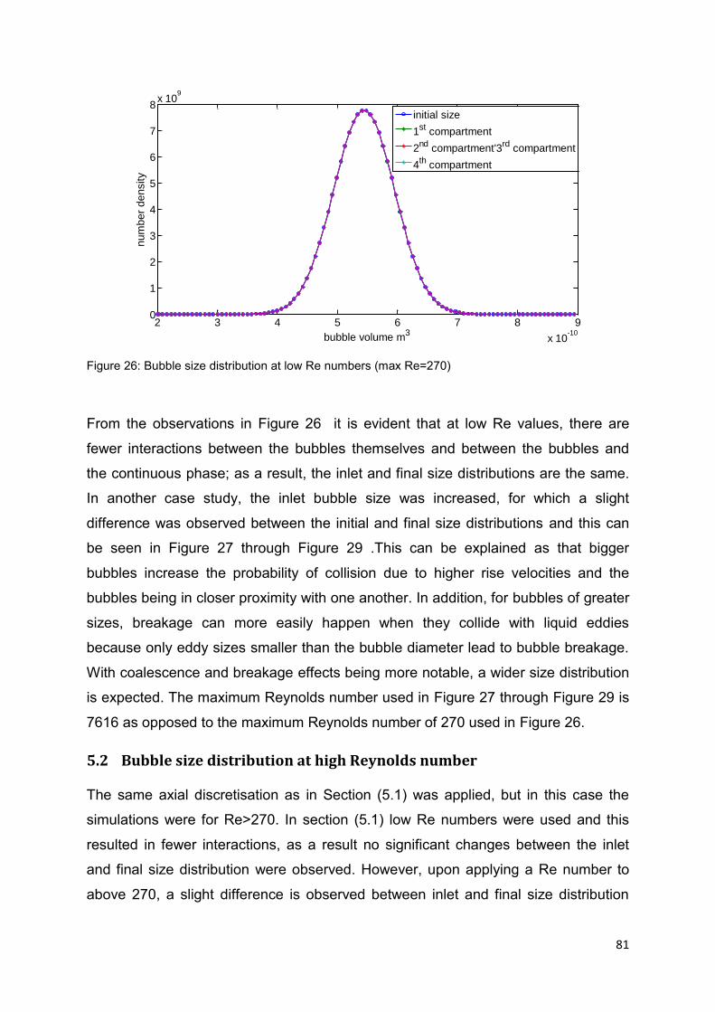
81

Figure 26: Bubble size distribution at low Re numbers (max Re=270)

From the observations in Figure 26 it is evident that at low Re values, there are

fewer interactions between the bubbles themselves and between the bubbles and

the continuous phase; as a result, the inlet and final size distributions are the same.

In another case study, the inlet bubble size was increased, for which a slight

difference was observed between the initial and final size distributions and this can

be seen in Figure 27 through Figure 29 .This can be explained as that bigger

bubbles increase the probability of collision due to higher rise velocities and the

bubbles being in closer proximity with one another. In addition, for bubbles of greater

sizes, breakage can more easily happen when they collide with liquid eddies

because only eddy sizes smaller than the bubble diameter lead to bubble breakage.

With coalescence and breakage effects being more notable, a wider size distribution

is expected. The maximum Reynolds number used in Figure 27 through Figure 29 is

7616 as opposed to the maximum Reynolds number of 270 used in Figure 26.

5.2 Bubble size distribution at high Reynolds number

The same axial discretisation as in Section (5.1) was applied, but in this case the

simulations were for Re>270. In section (5.1) low Re numbers were used and this

resulted in fewer interactions, as a result no significant changes between the inlet

and final size distribution were observed. However, upon applying a Re number to

above 270, a slight difference is observed between inlet and final size distribution

2 3 4 5 6 7 8 9

x 10-10

0

1

2

3

4

5

6

7

8x 10

9

bubble volume m3

nu

mb

er

de

nsity

initial size

1st

compartment

2nd

compartment'3rd

compartment

4th

compartment

82

and the distribution at the inlet compartment continues to change from compartment

to compartment. The Reynolds number was varied to a maximum of 7616 and the

findings in Figure 27 indicate that the bubble size distribution in the last column

compartment is slightly wider as compared to the inlet size distribution. A clear

representation of the difference between the initial and the final size distributions can

be observed in a case where the column is not compartmentalised as shown in

Figure 28. In this case it is evident that coalescence and breakage rates were slightly

higher, resulting in a slight difference between the final size distribution and the initial

size distribution. The number density probability distribution of the final size

distribution is also lower, indicating that the bubbles become fewer in number as they

coalesced along the column. An even more distinct difference between the initial and

final size distributions can be obtained in the case where a column height is

increased from 2 m to 3 m. In Figure 29, where the column height used is 3 m, it can

be observed that the final size distribution is wider and is characterised by both the

effects of breakage and coalescence being notable.

Figure 27: bubble size distribution along the column height

2 3 4 5 6 7 8 9

x 10-7

0

1

2

3

4

5

6

7

8x 10

6

bubble volume m3

nu

mb

er

de

nsity

initial size

1st

compartment

4th

compartment

83

Figure 28: Inlet and final size distributions (column height =2 m)

Figure 29: Inlet and final size distributions (column height =3 m)

The bubble size distribution differs slightly from one reactor compartment to another

as observed in Figure 27, Figure 28 and Figure 29. It is expected that at the regions

just above the sparger, the bubbles will be smaller in size and the bubble size

distribution to be narrow. As the bubbles rise in the column, coalescence and break

up occurs due to collision with the turbulent eddies, and the bubble size distribution

becomes wide with increasing column height. A reduction in bubble size also occurs

due to mass transfer from the gas-phase to the liquid phase. The loss of bubble size

due to mass transfer is represented by the expansion term in the Population Balance

2 3 4 5 6 7 8 9

x 10-7

0

1

2

3

4

5

6

7

8x 10

6

bubble volume m3

num

be

r d

ensity

initial size

final size

2 3 4 5 6 7 8 9

x 10-7

0

1

2

3

4

5

6

7

8x 10

6

bubble volume m3

nu

mb

er

de

nsity

initial size

final size

84

Equation. However, with coalescence occurring in parallel, the observations in

Figure 27 indicate overall, that at regions farther from the sparger, the bubbles

become bigger in size and fewer in number. The bubble size distribution presented

in Figure 28 and Figure 29 show that both coalescence and break up took place as

the final size distribution shows a wider distribution as compared to the inlet bubble

size distribution. The results attest to the fact that for tall columns, bubble size

distribution is wider as the bubbles have more time to coalesce and break up.

At this stage in the development, it is possible to develop the overall mass transfer

rate.

5.3 Overall mass transfer rate

In the design, scale-up and optimization of bubble columns, the rate of mass transfer

is the primary design variable. It is therefore crucial to develop models that can

reliably predict the mass transfer rate before unit design optimization can be

conducted. The Bubble Cell Model was used to predict the intrinsic mass transfer

coefficient for bubbles of different sizes in the column. As the BCM predicts

concentration gradients in the vicinity of a single bubble, the initial study consists of

the sensitivity of the mass transfer coefficient in the vicinity of a single bubble to Re

number with results shown in Figure 30. As expected, the mass transfer coefficient

increases with an increase in Re number. The increase can be attributed to

increased mixing and the advection terms dominating in the Navier- Stokes

equations at high Re numbers. As a result, the concentration boundary layer

thickness decreases which according to the film theory (see Equation 4.5) will cause

the mass transfer coefficient to increase. In addition, the increase of per-bubble

mass transfer rate with bubble size is attributed to increased interfacial fluctuations

and distortions. Although the bubble mass transfer coefficient has been predicted,

there is a need to predict the overall mass transfer rate for the column as shown by

Equation (5.3.1) .This is complicated by the hydrodynamics and the bubble geometry

characteristics. For the overall compartment mass transfer rate, the interfacial area

and bubble-averaged mass transfer coefficient are needed and this will be presented

in the sections to follow. The overall compartment mass transfer rate from the

population of bubbles in the column is presented in Table 9. The results show that

85

the overall compartment mass transfer is higher in the first compartment where the

bubbles are smaller in size and many in number.

Figure 30: Mass transfer coefficient in the vicinity of a single bubble at various Re numbers

(5.3.1)

Table 9: Overall compartment mass transfer rate along the column compartments

Total mass transfer rate as calculated from BCM (max Re=240)

compartment 1 2 3 4

Ntot, model prediction

(kmol/s)

4.813x10-6 2.401x10-6 2.398x10-6 2.394x10-6

For a better understanding of mass transfer, it is necessary to investigate the factors

which influence the intrinsic mass transfer coefficient such as turbulent energy

dissipation rate, bubble slip velocity, bubble size distribution, and bubble breakup

and coalescence (Wang, 2010). The factors investigated in the current study are

bubble size, axial position and Re number.

100 120 140 160 180 200 220 240 260 2805

5.5

6

6.5

7

7.5x 10

-5

Reynolds number

Ma

ss t

ransfe

r co

eff

icie

nt

(m/s

)

86

5.3.1 The relationship between the bubble size, axial position and the mass transfer

coefficient

The rate of mass transfer in a column depends primarily on the specific interfacial

area (a) and the intrinsic liquid-phase mass transfer coefficient (kL). In the

determination of what the mass transfer rate will be in the column, it is crucial to

decouple (kL) from (a). This is important as it can be determined if the changes in the

interfacial area will be greater than the changes in the intrinsic mass transfer

coefficient, and, as a result, the controlling rate in the column can be determined.

The influence of bubble size on the mass transfer coefficient was investigated by

changing the inlet bubble size distribution and predicting the average mass transfer

coefficient in each case (see Equation 5.2).

The results in Figure 31 indicate that the intrinsic mass transfer coefficient increases

with bubble size as the bigger bubbles have higher Re number than smaller bubbles,

and this is in agreement with published findings on the effect of bubble size on mass

transfer coefficient (Miller, 1983). According to this research, the mass transfer

coefficient is dependent on mean bubble size and it increases with increasing bubble

size.

With respect to the mass transfer coefficient averaged over space in the vicinity of a

bubble, the observations are that like the intrinsic mass transfer coefficient, it

increases with an increase in bubble size as observed in Figure 32. The increase of

mass transfer coefficient along the column height can be explained by coalescence

being more dominant as we move to the top of the column and thus yielding large

bubbles which have high Reynolds number. Although the mass transfer coefficient

increases with column height due to increased bubble size, the overall mass transfer

rate decreases due to relatively smaller interfacial area of larger bubbles as

compared to smaller bubbles. This can be observed in Table 9 where the overall

mass transfer rate along the column compartments is presented.

The smaller bubbles, which are found at the regions near the sparger tend to

behave like rigid spheres and encounter a hindered flow in the boundary layer sense

due to frictional drag, and, as a result, the intrinsic mass transfer coefficient is lower

(Nedeltchev & Schumpe .,2011, Oliveira & Ni, 2004). On the other hand, the larger

bubbles have higher rise velocities and mobile surfaces and as a result experience

87

significant fluid circulation and thus higher intrinsic mass transfer coefficient. The

findings in the current study are consistent to the work of Nedeltchev & Schumpe

(2011) and Oliveira & Ni (2004) as observed in Figure 31 and Figure 32.

The local mass transfer coefficient in the vicinity of individual bubbles is presented in

Figure 33 and the same trends as for the bubble average and intrinsic mass transfer

coefficient are observed. The results presented in Figure 33 are for the individual

bubbles in the first column compartment.

Figure 31: Intrinsic mass transfer coefficient at various column compartments

Figure 32: Bubble Averaged mass transfer coefficient at various column compartments

2 3 4 5 6 7 8 9 10

1.24

1.25

1.26

1.27

1.28

1.29

1.3

1.31x 10

-3

Column height (m)

Intr

insic

mass t

ransfe

r coeff

icie

nt

(m/s

)

2 3 4 5 6 7 8 9 101.22

1.24

1.26

1.28

1.3

1.32

1.34x 10

-3

Column height (m)

Avera

ge m

ass t

ransfe

r coeff

icie

nt

(m/s

)

88

Figure 33: Local mass transfer coefficient in the vicinity of individual bubbles

5.4 Sensitivity analysis

A sensitivity analysis is performed by investigating the system response to changes

in model parameters. It is important in that it gives an insight into the relevance of

including certain phenomena to the model. The sensitivity analysis establishes the

operating regions associated with specific behaviour patterns and allows for an

understanding of the system dynamics. In the current study, the parameters of

interest include column dimensions and inlet bubble size distribution. In each

sensitivity analysis carried out, the results were compared with the findings from the

literature.

5.4.1 The influence of column dimensions on gas hold-up

The accurate prediction of gas hold-up is of paramount importance due to its

significant influence on the performance of bubble columns. It is asserted that it

indirectly governs the liquid phase flow, and ultimately the rates of mixing, heat and

mass transfer (Wu, Cheng Ong & Al-Dahhan, 2001). In the absence of liquid

recirculation, gas hold-up is directly proportional to residence time. In terms of

column operation, a high level of gas hold-up results in greater gas-liquid contact. In

the current study, gas hold-up was predicted by the Population Balance Equation

using bubble size distribution as illustrated in Equation 2.4.

2 3 4 5 6 7 8 9 10

x 10-8

0

0.5

1

1.5

2

2.5

3x 10

-3

Bubble volume (m3)

Lo

ca

l in

trin

sic

ma

ss t

ransfe

r co

eff

icie

nt

(m/s

)

89

The influence of column dimension on gas hold-up was investigated by varying the

column diameter or column height and reporting the findings in each case. By

changing the column diameter, the gas hold-up in each chosen reactor compartment

was found to remain constant. As illustrated in Table 10, the constant gas hold-up

upon changing the column diameter can be attributed to the constant bubble

residence time in the absence of liquid recirculation. In the absence of liquid

recirculation, the terminal velocity can be directly related to residence time; hence

bigger bubbles are expected to have smaller gas hold up due to their high rise

velocities. In addition, the coalescence and break-up models show a dependence on

the column geometry; physically, the cross-sectional area relates to the probability

that bubbles will collide, the column dimensions therefore influence the frequency of

the events. In spite of the aforementioned criterion, it is the column height that shows

the strong influence on gas hold-up as shown in Table 11, whilst the change in the

column diameter does not result in the change in gas hold-up.

The observations in Table 11 show that the gas hold-up increases upon increasing

the column height. The increase in gas hold-up can be attributed to longer residence

times in tall columns and in the absence of liquid recirculation (which is the case in

the current study), gas hold-up is directly proportional to the residence time. Seeing

that the gas hold-up is sensitive to these values of column height, an exaggerated

column height of 20 m was attempted to investigate further the influence of column

height; in this region gas hold-up does indeed become a strong function of column

height due to the increased time of exposure of the bubbles to breakup and

coalescence phenomena and also due to an increased bubble residence time. The

influence of the axial position (at fixed column height) on gas hold-up was also

investigated and the findings are as shown in Table 11. The observations indicate

that gas hold-up decreases with an increase in axial position, as observed in Table

11 that it decreases from one compartment to another. This can be explained by the

decrease in bubble residence time as they rise through the column from one

compartment to the next, due to their sizes becoming bigger as a result of

coalescence.

On the study of the effect of aspect ratio on gas hold-up, Daly et al. (1992) found that

gas hold up is independent on column height, whilst column diameter results in some

changes in gas hold up. They found that gas hold up in a small diameter column was

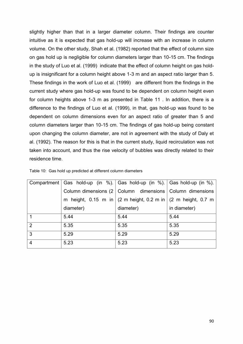
90

slightly higher than that in a larger diameter column. Their findings are counter

intuitive as it is expected that gas hold-up will increase with an increase in column

volume. On the other study, Shah et al. (1982) reported that the effect of column size

on gas hold up is negligible for column diameters larger than 10-15 cm. The findings

in the study of Luo et al. (1999) indicate that the effect of column height on gas hold-

up is insignificant for a column height above 1-3 m and an aspect ratio larger than 5.

These findings in the work of Luo et al. (1999) are different from the findings in the

current study where gas hold-up was found to be dependent on column height even

for column heights above 1-3 m as presented in Table 11 . In addition, there is a

difference to the findings of Luo et al. (1999), in that, gas hold-up was found to be

dependent on column dimensions even for an aspect ratio of greater than 5 and

column diameters larger than 10-15 cm. The findings of gas hold-up being constant

upon changing the column diameter, are not in agreement with the study of Daly et

al. (1992). The reason for this is that in the current study, liquid recirculation was not

taken into account, and thus the rise velocity of bubbles was directly related to their

residence time.

Table 10: Gas hold up predicted at different column diameters

Compartment Gas hold-up (in %).

Column dimensions (2

m height, 0.15 m in

diameter)

Gas hold-up (in %).

Column dimensions

(2 m height, 0.2 m in

diameter)

Gas hold-up (in %).

Column dimensions

(2 m height, 0.7 m

in diameter)

1 5.44 5.44 5.44

2 5.35 5.35 5.35

3 5.29 5.29 5.29

4 5.23 5.23 5.23

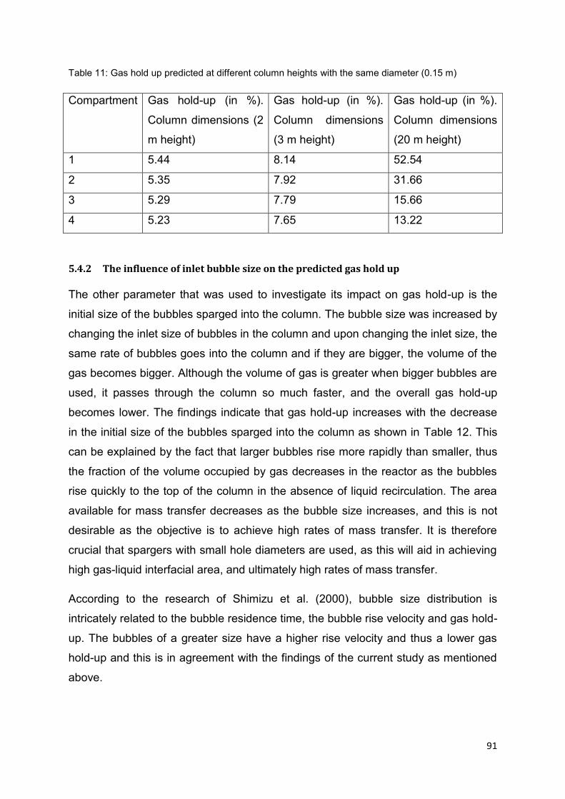
91

Table 11: Gas hold up predicted at different column heights with the same diameter (0.15 m)

Compartment Gas hold-up (in %).

Column dimensions (2

m height)

Gas hold-up (in %).

Column dimensions

(3 m height)

Gas hold-up (in %).

Column dimensions

(20 m height)

1 5.44 8.14 52.54

2 5.35 7.92 31.66

3 5.29 7.79 15.66

4 5.23 7.65 13.22

5.4.2 The influence of inlet bubble size on the predicted gas hold up

The other parameter that was used to investigate its impact on gas hold-up is the

initial size of the bubbles sparged into the column. The bubble size was increased by

changing the inlet size of bubbles in the column and upon changing the inlet size, the

same rate of bubbles goes into the column and if they are bigger, the volume of the

gas becomes bigger. Although the volume of gas is greater when bigger bubbles are

used, it passes through the column so much faster, and the overall gas hold-up

becomes lower. The findings indicate that gas hold-up increases with the decrease

in the initial size of the bubbles sparged into the column as shown in Table 12. This

can be explained by the fact that larger bubbles rise more rapidly than smaller, thus

the fraction of the volume occupied by gas decreases in the reactor as the bubbles

rise quickly to the top of the column in the absence of liquid recirculation. The area

available for mass transfer decreases as the bubble size increases, and this is not

desirable as the objective is to achieve high rates of mass transfer. It is therefore

crucial that spargers with small hole diameters are used, as this will aid in achieving

high gas-liquid interfacial area, and ultimately high rates of mass transfer.

According to the research of Shimizu et al. (2000), bubble size distribution is

intricately related to the bubble residence time, the bubble rise velocity and gas hold-

up. The bubbles of a greater size have a higher rise velocity and thus a lower gas

hold-up and this is in agreement with the findings of the current study as mentioned

above.

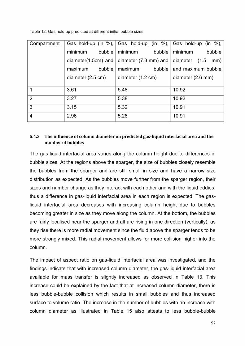
92

Table 12: Gas hold up predicted at different initial bubble sizes

Compartment Gas hold-up (in %),

minimum bubble

diameter(1.5cm) and

maximum bubble

diameter (2.5 cm)

Gas hold-up (in %),

minimum bubble

diameter (7.3 mm) and

maximum bubble

diameter (1.2 cm)

Gas hold-up (in %),

minimum bubble

diameter (1.5 mm)

and maximum bubble

diameter (2.6 mm)

1 3.61 5.48 10.92

2 3.27 5.38 10.92

3 3.15 5.32 10.91

4 2.96 5.26 10.91

5.4.3 The influence of column diameter on predicted gas-liquid interfacial area and the

number of bubbles

The gas-liquid interfacial area varies along the column height due to differences in

bubble sizes. At the regions above the sparger, the size of bubbles closely resemble

the bubbles from the sparger and are still small in size and have a narrow size

distribution as expected. As the bubbles move further from the sparger region, their

sizes and number change as they interact with each other and with the liquid eddies,

thus a difference in gas-liquid interfacial area in each region is expected. The gas-

liquid interfacial area decreases with increasing column height due to bubbles

becoming greater in size as they move along the column. At the bottom, the bubbles

are fairly localised near the sparger and all are rising in one direction (vertically); as

they rise there is more radial movement since the fluid above the sparger tends to be

more strongly mixed. This radial movement allows for more collision higher into the

column.

The impact of aspect ratio on gas-liquid interfacial area was investigated, and the

findings indicate that with increased column diameter, the gas-liquid interfacial area

available for mass transfer is slightly increased as observed in Table 13. This

increase could be explained by the fact that at increased column diameter, there is

less bubble-bubble collision which results in small bubbles and thus increased

surface to volume ratio. The increase in the number of bubbles with an increase with

column diameter as illustrated in Table 15 also attests to less bubble-bubble

93

collisions in a larger column diameter. The presence of many bubbles in a larger

column diameter can be attributed to the prevalence of liquid recirculation and

turbulence, which in turn results in many bubbles which are smaller in size. On the

contrary, for a small column diameter, a slug flow regime is encountered and this

results in bigger bubbles being dominant and thus fewer in number as the results in

Table 15 indicate. It can also be concluded that the rate of coalescence is greater

than that of break up in the case of a small diameter column and this is manifested

by the presence of fewer bubbles. In a wider diameter column, the presence of many

bubbles can be explained by the more lateral space which minimises the chances of

collision and coalescence.

The increase of aspect ratio by changing the column height shows a more significant

change as compared to changing the column diameter. This can be observed in

Table 14 where the findings show interfacial area to decrease as the column height

is increased. The explanation lies in the fact that for tall columns, there is more

contact time between the bubbles which enhances coalescence hence reduced

interfacial area. The change in column height shows that, although there are some

observed changes in interfacial area, the interfacial area is not a strong function of

column height. In view of that, an exaggerated column height of 20 m was attempted

and at this height the observations show that the interfacial area has a strong

dependence on column height.

Table 13: Interfacial area predicted at different column diameters

Compartment Interfacial area(m2/m3)

Column dimensions (2

m height, 0.15 m in

diameter)

Interfacial

area(m2/m3) Column

dimensions (2 m

height, 0.2 m in

diameter)

Interfacial

area(m2/m3) Column

dimensions (2 m

height, 0.01 m in

diameter)

1 33.08 33.08 32.23

2 32.49 32.49 32.14

3 32.13 32.13 31.62

4 31.75 31.75 31.25

94

Table 14: Interfacial area predicted at different column heights

Compartment Interfacial area(m2/m3)

Column dimensions (1

m height, 0.15 m in

diameter)

Interfacial

area(m2/m3) Column

dimensions (3 m

height, 0.15 m in

diameter)

Interfacial

area(m2/m3)

Column dimensions

(20 m height, 0.15

m in diameter)

1 33.18 32.97 32.32

2 32.89 32.06 19.39

3 32.71 31.54 9.57

4 32.52 30.96 8.05

Table 15: Number of bubbles predicted at different column diameters

Compartment Number of bubbles. Column

dimensions (2 m height, 0.2 m

in diameter)

Number of bubbles. Column

dimensions (2 m height, 0.7 m

in diameter)

1 1.60x103 1.96x104

2 1.57x103 1.93x104

3 1.56x103 1.91x104

4 1.54x103 1.88x104

5.4.4 The influence of the expansion term on the predicted mean diameter

The inclusion of the expansion term in the Population Balance Equation, takes into

account the reduction of bubble size due to mass transfer into the liquid phase. It is

therefore expected that the exclusion of this term will result in the predicted bubble

size being larger than when it is included. In the current study, the findings in

excluding the expansion term indicate that the mean bubble size in each reactor

compartment is slightly bigger than when the term is included as observed in Table

16. It was observed that the exclusion of the expansion term results in the same

bubble size distribution to when it is included and this observation is illustrated in

Figure 34 and Figure 35. The sensitivity to the inclusion of this effect is negligible.

The difference between the Sauter mean diameters predicted in each case is

insignificant, and this can be attributed to the low rates of mass transfer due to poor

95

mixing at low Re numbers as it was in this case. Although the effect of mass transfer

on the predicted bubble size is insignificant, in the current model it was included as

its effect would be more notable at higher Re numbers.

Table 16: The predicted Sauter mean diameter with and without mass transfer consideration

compartment Sauter mean diameter(m)

With mass transfer consideration

Sauter mean diameter(m) Without

mass transfer consideration

1 1.018x10-2 1.018x10-2

2 1.0170x10-2 1.018x10-2

3 1.016x10-2 1.018x10-2

4 1.016x10-2 1.018x10-2

Figure 34: bubble size distribution with the inclusion of mass transfer term in the bubble PBM

equation (Max Re=7616)

2 3 4 5 6 7 8 9

x 10-7

0

1

2

3

4

5

6

7

8x 10

6

bubble volume m3

nu

mb

er

de

nsity

initial size

1st

compartment

4th

compartment

96

Figure 35: bubble size distribution with the exclusion of mass transfer term in the bubble PBM

equation (Max Re=7616)

5.5 Predicting heat transfer coefficients

The overall Heat transfer coefficient was predicted from mass transfer results by

applying the analogy between heat and mass transfer as explained in section (2.1.8).

The accuracy of the analogy in predicting the intrinsic heat transfer coefficient was

benchmarked by comparing the heat transfer coefficient predicted from CFD and the

one predicted from heat and mass analogy. Close agreement is found as shown in

Figure 18. The heat transfer coefficient in each column compartment was

determined by averaging heat transfer coefficient results from all the bubbles in that

respective compartment. The averaging was perfomed using the number density

probability distribution and heat transfer coefficient for all bubbles in the

compartment and it was calculated as shown in Equation (5.5.1).

∫

(5.5.1)

As intimated above, the heat transfer coefficient for a population of bubbles in the

column was determined and the results are shown in Figure 36. The findings indicate

that with an increase in bubble size, the predicted heat transfer coefficient

2 3 4 5 6 7 8 9 10

x 10-7

0

1

2

3

4

5

6

7

8x 10

6

bubble volume m3

nu

mb

er

de

nsity

initial size

1st

compartment

4th

compartment

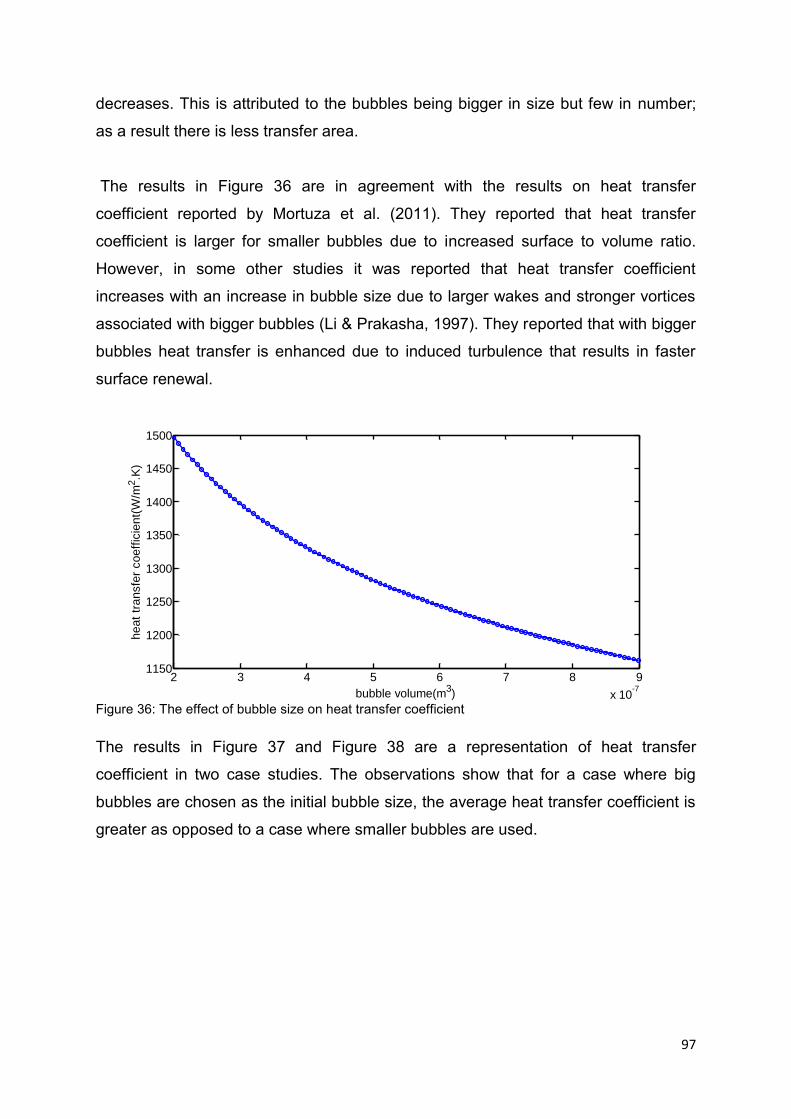
97

decreases. This is attributed to the bubbles being bigger in size but few in number;

as a result there is less transfer area.

The results in Figure 36 are in agreement with the results on heat transfer

coefficient reported by Mortuza et al. (2011). They reported that heat transfer

coefficient is larger for smaller bubbles due to increased surface to volume ratio.

However, in some other studies it was reported that heat transfer coefficient

increases with an increase in bubble size due to larger wakes and stronger vortices

associated with bigger bubbles (Li & Prakasha, 1997). They reported that with bigger

bubbles heat transfer is enhanced due to induced turbulence that results in faster

surface renewal.

Figure 36: The effect of bubble size on heat transfer coefficient

The results in Figure 37 and Figure 38 are a representation of heat transfer

coefficient in two case studies. The observations show that for a case where big

bubbles are chosen as the initial bubble size, the average heat transfer coefficient is

greater as opposed to a case where smaller bubbles are used.

2 3 4 5 6 7 8 9

x 10-7

1150

1200

1250

1300

1350

1400

1450

1500

bubble volume(m3)

he

at

tra

nsfe

r co

eff

icie

nt(

W/m

2.K

)

98

Figure 37: The variation of heat transfer coefficient along the column height at bigger bubbles chosen

as initial sizes (minimum size (7.3 mm) and maximum size (1.2 cm))

Figure 38: The variation of heat transfer coefficient along the column height at smaller bubbles

chosen as initial sizes (minimum size (0.73 mm) and maximum size (1.2 mm))

5.6 Model validation

Model validation was conducted by comparing the results of the predicted gas hold-

up, interfacial area and heat transfer coefficient against the results predicted by

correlations reported in the literature.

1 1.5 2 2.5 3 3.5 4

1262.85

1262.9

1262.95

1263

1263.05H

ea

t tr

ansfe

r co

eff

icie

nt(

W/m

2.K

)

column compartment

1 1.5 2 2.5 3 3.5 44048

4049

4050

4051

4052

4053

4054

4055

He

at

tra

nsfe

r co

eff

icie

nt(

W/m

2.K

)

column compartment

99

5.6.1 Validating gas hold-up

The model results on gas hold-up were validated against correlations reported in the

literature. There are several correlations for the prediction of gas hold-up and of the

ones chosen for model validation, it can be seen from Figure 39 that the correlations

by Reilly et.al (1986) and Kelkar et.al (1983) show a good agreement to the model

results. We note that these correlations were chosen for comparison with model

results since they involve the same basic chemicals (air and water). Equations 5.3-

5.5 are the mathematical expressions for the correlations of gas hold-up used for

model validation. The predicted values for gas hold-up are very close to the

correlations in the literature as illustrated in Figure 39.

𝑈

√

(5.3)

4 5

(5.4)

𝜎

(5.5)

Figure 39: Comparison of the model results to the correlation results

1 1.5 2 2.5 3 3.5 40.066

0.0665

0.067

0.0675

0.068

0.0685

compartment number

ga

s h

old

-up

model

Winkler(1981)

Kelkar (1983)

Reilly(1986)

100

5.8.2 Validating interfacial area

The specific interfacial area available for mass transfer was also validated using

correlations reported in the literature. The correlation used in validating interfacial

area is by Serizawa & Kataoka,. (1989). The correlation was used because it was

derived for an air-water system and the current work is focusing on the same

system. The results in Table 17 show that there is a 29 % discrepancy between the

model results and the results calculated from the interfacial area correlation.

However, upon decreasing the inlet bubble size as shown in Table 18, the findings

indicate that there is a close agreement between the model results and the results

predicted from the correlation. The explanation for the model results yielding a close

agreement to the correlations at certain operating conditions can be ascribed to the

accuracy of the correlations which is only maintained under the conditions in which

they were derived. The correlation against which the model was validated has the

mathematical formulation presented in Equation 5.6.

3 𝑈

(5.6) Table 17: Validating interfacial area (bubble sizes ranging from 7.3 mm to 1.2 cm)

compartment Model Prediction of interfacial area (m2/m3)

interfacial area calculated from the correlation by (m2/m3)

Relative error (%)

1 33.08 46.42 28.74 2 32.49 45.70 28.91 3 32.13 45.27 29.01 4 31.75 44.80 29.12 The validation of interfacial area demonstrated in Table 17 is for bubble sizes

ranging from 7.33 mm to 1.2 cm and upon using bigger bubble sizes, a close

agreement to the results predicted by the correlation is found as shown in Table 18.

101

Table 18: Validating interfacial area (bubble sizes ranging from 2.4 mm to 8.8 mm)

compartment Model Prediction of interfacial area (m2/m3)

interfacial area calculated from the correlation(m2/m3)

Relative error (%)

1 22.71 23.43 3.07 2 22.29 23.05 3.30 3 22.03 22.82 3.45 4 21.76 22.57 3.61

Since interfacial area and gas hold-up have been validated against correlations, the

Sauter mean diameter was not validated because gas hold-up was calculated from

interfacial area and Sauter mean diameter as follows:

(5.7)

Therefore a close agreement between the interfacial area and gas hold-up results

with the results calculated from the correlations, gives surety that the predicted mean

diameter is accurate as well.

5.8.3. Validating heat transfer coefficient

The heat transfer coefficient predicted from the heat and mass analogy was

validated against heat transfer coefficient correlations reported in the literature. The

correlations by Whitaker (1972) and Clift et.al (1978) are expressed mathematically

as follows:

5 (

)

(5.8)

( 4√ )

(5.9)

The Nusselt number calculated from the correlations as shown in equations (5.8)

and (5.9) was compared with the Nusselt number calculated from the heat and mass

analogy as illustrated in Table 19 . The findings indicate that the correlation by

102

Whitaker (1972) shows a better agreement to the model results as compared to the

correlation by Clift.et.al (1978).

Table 19: Validating the Nusselt number calculated from the model against correlations

Compartment number

Average Nusselt number calculated from heat and mass analogy

Average Nusselt number from the correlation by Clift el.al (1978) with relative errors in parentheses

Average Nusselt number from the correlation by Whitaker el.al (1972) with relative errors in parentheses

2 54.358 41.496 (23.661) 45.986 (15.402)

3 54.345 41.492 (23.651) 45.980 (15.393)

4 54.332 41.487 (23.641) 45.974 (15.383)

5.8.4 Validating mass transfer results

As outlined in the previous sections, mass transfer from the dispersed to the

continous phase was predicted from the Bubble Cell Model and the accuracy of the

results predicted was tested against the experimental data by the use of reported

correlations as presented in Table 20. The predicted mass transfer rate was

validated against the mass transfer rate predicted from the correlation by Ranz

&Marshal, (1952) and a close agreement was achieved with an average relative

error of ±6 %. Some other correlations showed a pronounced departure from the

model and the explanation lies in the fact the emperical correlations are limited in

their prediction as they are accurate under the conditions in which they were derived,

and depend also in other parameters like equipment type and geometry. The

fundamental model was used in the current study and experiments were not needed.

103

Table 20: Validation of mass transfer results

Compartment number

Total mass transfer rate from model prediction (Kmol/s)

Total mass transfer rate from the correlation by (Ranz and Marshal,1952) (Kmol/s)

Relative error (%)

2 1.155x10-6 1.080x10-6 6.491 3 1.145x10-6 1.076x10-6 6.071 4 1.136x10-6 1.072x10-6 5.648

5.9 Model speed test

A speed test was performed to evaluate whether the current model is quicker as

compared to other models. Using MATLAB 2011, it took 15.82 seconds for the

current model to predict the parameters of interest by integration of BCM into the

PBM framework. When using the same grid points in CFD to get the converged

numerical solutions for the prediction of mass transfer coefficient, it took 1.46

minutes. It could therefore be seen that the integration of BCM into the PBM

framework is extremely fast compared to some conventional CFD modelling

techniques. In addition, good predictions were also achieved as seen from

comparing the model results with empirical correlations.

5.10 Summary

The model gives accurate predictions at higher speeds than the existing models.

However, it is limited to low Re numbers; to become more general, the BCM itself

must be developed to account for the change in bubble shape, and that is beyond

the scope of the present study. However, even the result from the present study is

significant since it takes any general bubble column simulation and, for the regions

where the Re value is low, this method can be applied to speed up the calculation for

that fraction of the fluid

104

Chapter 6

6. Concluding remarks

A model for predicting hydrodynamic variables in a bubble column was developed by

integrating the BCM into the PBM framework. The Bubble Cell Model has the ability

to rapidly predict velocity gradients (Coetzee et al., 2011), heat and mass transfer

coefficients, and has an advantage that in its predictive ability, it does not depend on

operating conditions and equipment type. The integration of BCM into the Population

Balance framework is therefore a fundamental approach as the BCM is generic in its

predictive nature.

The limitation in the application of BCM is the range of Re numbers used (maximum

Re number being 270). At low Reynolds numbers the bubble size distribution along

the column does not change due to the absence of bubble-bubble interaction and

eddy-bubble interaction, rendering Population Balances superfluous. However, at

high Re numbers there is increased interaction between the dispersed and the

continuous phase and bubble size distribution varies along the column, thus the

Population Balance Equation needs to be employed. The current work aimed at

integrating the BCM into the PBM framework, and BCM in its current development

can only be employed to a maximum Re number of 270, and at these Re numbers

the bubble size distribution does not change along the column height as shown in

section 5. It is therefore vital to extend BCM to high Re numbers as in its current

development, its integration into the PBM framework does not achieve the intended

purpose since at low Re numbers there is no significant difference between the initial

and final size distributions. The current work therefore focusses on answering

whether it is worth the intellectual investment to develop extensions to the BCM for

higher Re values. To answer this question, in the regions where BCM does yield

accurate answers, the computational expense was benchmarked against the

traditional CFD approaches.

The predicted hydrodynamic variables are mass and heat transfer coefficients, gas

hold-up, interfacial area and Sauter mean diameter. The predicted hydrodynamic

variables were validated against correlations and a good agreement was found

105

between the results predicted from the model and the correlations. The predicted

parameters showed a close agreement with the correlations with overall gas hold-up

having an error of ±0.6 %, interfacial area ±3.36 % and heat transfer coefficient

±15.4 %. On the computational expense, a speed test was performed to evaluate

whether the current model is quicker as compared to other models. Using MATLAB

2011, it took 15.82 seconds for the current model to predict the parameters of

interest by integration of BCM into the PBM framework. When using the same grid

points in CFD to get the converged numerical solutions for the prediction of mass

transfer coefficient, it took 1.46 minutes. It could therefore be concluded that the

integration of BCM into the PBM framework is extremely fast compared to some

conventional CFD modelling techniques

In addition, this approach allowed for deconvolution of the interfacial area and mass

transfer coefficient, thereby advancing the understanding of the mass transfer

mechanisms and also enabling determination of the controlling rate in the column.

The aforementioned parameters were predicted separately as the volumetric mass

transfer coefficient which is normally used in mass transfer predictions, does not

allow for the decoupling of mass transfer mechanisms .The findings in the current

study indicate that interfacial area controls the rate of mass transfer as intimated in

section 5. On the other hand, the findings indicate that gas hold-up is bigger for small

bubbles as they rise slowly in the column compared to the bigger bubbles. The

current study did not take into account liquid recirculation in the column, thus bubble

residence time was directly related to bubble rise velocity, and hence low gas hold-

ups were found for high bubble rise velocities.

On the investigation of the influence of column dimensions on the predicted

hydrodynamics, the small diameter column resulted in bigger bubble sizes due to the

slug flow that is encountered. In a small diameter column, the mass transfer rates

are low due to decreased interfacial area. However, in the current study the column

diameter was found to not be a strong function of the hydrodynamics parameters as

observed in section 5. On the contrary, the hydrodynamic variables change with the

column height. For instance, upon increasing the column diameter, the mean bubble

size was found to increase as well, thus decreasing gas hold-up as mentioned

earlier.

106

The heat transfer coefficient was predicted from mass transfer coefficient results

using the analogy that exists in the mathematical formulation of the two parameters,

and the predicted heat transfer coefficient was validated against correlations and

was found to be in good agreement. It is important to note that though the predicted

hydrodynamic parameters showed a good agreement to the results predicted from

the correlations, this can only be achieved at certain operating conditions. Upon

changing the operating conditions such as Re number, column diameter or height

and the superficial gas velocity, there is an observed deviation between model

results and those predicted from correlations. The deviation can be attributed to the

limitation of correlations as they can only yield accurate results under conditions in

which they were derived, beyond those operating conditions their accuracy can no

longer be maintained.

From the intimated observations, it can be concluded that due to the savings on

computational expense at low Re values, it would be worth the intellectual expense

to extend BCM to higher Re values. Although BCM is limited to low Re values, the

result from the present study is significant since it takes any general bubble column

simulation and, for the regions where the Re value is low, this method can be applied

to speed up the calculation for that fraction of the fluid. The additional advantages

are that the intrinsic mass coefficient and specific interfacial area calculated allowing

for more detailed designs. In addition, the intrinsic mass transfer coefficient and the

specific interfacial area were determined independently and that allows for the

decoupling of mass transfer mechanisms.

6.1. Recommendations

Bubble Cell Model predicts the velocity, temperature and concentration fields in the

vicinity of a single bubble and it is extremely fast in its predictive capability. On the

other hand, the Population Balance Model predicts the distribution of discrete

entities. Since the BCM predicts the aforementioned parameters in the vicinity of a

single bubble, the information from the BCM was used to calculate the distribution of

the parameters for a population of bubbles in the column. This was done by

integrating BCM into the Population Balance framework. There is a limitation in the

use of BCM since it can only be employed to maximum Re number of 270 and it was

observed in the current study that in this range of Re numbers, size distribution does

107

not change along the column and the integration of BCM into the Population Balance

framework is not necessary. However, upon increasing Re numbers, bubble size

distribution along the column changes and it is at these high Re numbers that the

integration of BCM into the Population Balance framework is essential. Therefore the

extension of BCM to high Re number is crucial. The other extension to the BCM-

PBM application can be the studying of reactive systems.

In the current study, the bubble residence time was directly related to bubble rise

velocity as liquid recirculation was not considered. The model prediction can be

improved by considering liquid recirculation and the different angles at which bubbles

rise in the column, and thus velocity distribution can be modelled from BCM-PBM

approach. The bubble rise velocity is a function of bubble size and PBM has the

ability to predict bubble size, thus knowing bubble size as a function of position and

time, the velocity distribution can be calculated from macroscopic force balance.

108

7. References

Abdulmohsin, R.S., Abid, B.A. & Al-Dahhan, M.H. 2011. Heat transfer study in a pilot-plant scale bubble column. Chemical engineering research and design. 89(1):78-84. DOI:10.1016/j.cherd.2010.04.019.

Atika,K., Yoshida,F.1973. Gas hold-up and volumetric mass transfer coefficient in bubble columns. Ind. Eng. Chem.12:76-80

Azzopardi, B.J., Mudde, R.F., Lo, S., Morvan, H., Yan, Y.Y & Zhao, D. 2011. Hydrodynamics of Gas-Liquid Reactors. John Wiley & Sons Ltd.

Bannari, R., Kerdouss, F., Selma, B., Bannari, A. & Proulx, P. 2008a. Three-dimensional mathematical modeling of dispersed two-phase flow using class method of population balance in bubble columns. Computers & chemical engineering. 32(12):3224-3237. DOI:10.1016/j.compchemeng.2008.05.016.

Bannari, R., Kerdouss, F., Selma, B., Bannari, A. & Proulx, P. 2008b. Three-dimensional mathematical modeling of dispersed two-phase flow using class method of population balance in bubble columns. Computers & chemical engineering. 32(12):3224-3237. DOI:10.1016/j.compchemeng.2008.05.016.

Batchelor, G.K., 1967. An Introduction to Fluid Dynamics. Cambridge University Press. 15, 24,60

Bayraktar, E., Mierka, O., Platte, F., Kuzmin, D. & Turek, S. 2011. Numerical aspects and implementation of population balance equations coupled with turbulent fluid dynamics. Computers & chemical engineering. 35(11):2204-2217. DOI:10.1016/j.compchemeng.2011.04.001.

Bhole, M.R., Joshi, J.B. & Ramkrishna, D. 2008. CFD simulation of bubble columns incorporating population balance modeling Chemical engineering science. 63(8):2267 <last_page> 2282. DOI:10.1016/j.ces.2008.01.013.

Bouaifi, M., Hebrard, G., Bastoul, D. & Roustan, M. 2001. A comparative study of gas hold-up, bubble size, interfacial area and mass transfer coefficients in stirred gas–liquid reactors and bubble columns. Chemical engineering and processing: Process intensification. 40(2):97-111. DOI:10.1016/S0255-2701(00)00129-X.

Brenner, C.E. 2005. Fundamentals of multiphase flow. New York. Cambridge University Press

Chaumat, H., Billet-Duquenne, A.M., Augier, F., Mathieu, C. & Delmas, H. 2005. Mass transfer in bubble column for industrial conditions—effects of organic medium, gas and liquid flow rates and column design. Chemical engineering science. 60(22):5930-5936. DOI:http://dx.doi.org/10.1016/j.ces.2005.04.026.

Chen, P., Sanyal, J. & Dudukovic, M. 2005. Numerical simulation of bubble columns flows: effect of different breakup and coalescence closures. Chemical engineering science. 60(4):1085-1101.

Chesters, A.K. 1991. Modelling of coalescence processes in fluid-liquid dispersions. A review of current understanding. Chemical engineering research and design. 69(4):259-227.

109

Clift, R., Grace, J.R. & Weber, M.E. 1978. Bubbles drops and particles. New York: Academic Press

Coetzee, W., Coetzer, R.L.J. & Rawatlal, R. Response surface strategies in constructing statistical bubble flow models for the development of a novel bubble column simulation approach. Computers & chemical engineering. (0) DOI:10.1016/j.compchemeng.2011.07.014.

Colombet, D., Legendre, D., Cockx, A., Guiraud, P., Risso, F., Daniel, C. & Galinat, S. 2011. Experimental study of mass transfer in a dense bubble swarm. Chemical engineering science. 66(14):3432-3440. DOI:http://dx.doi.org/10.1016/j.ces.2011.01.020.

Daly, J.G., Patel, S.A. & Bukur, D.B. 1992. Measurement of gas holdups and sauter mean bubble diameters in bubble column reactors by dynamics gas disengagement method. Chemical engineering science. 47(13–14):3647-3654. DOI:10.1016/0009-2509(92)85081-L.

Degaleesan, S., Dudukovic, M. & Pan, Y. 2001. Experimental study of gas-induced liquid-flow structures in bubble columns. AIChE journal. 47(9):1913-1931. DOI:10.1002/aic.690470904.

Delnoij, E., Lammers, F.A., Kuipers, J.A.M. & van Swaaij, W.P.M. 1997. Dynamic simulation of dispersed gas-liquid two-phase flow using a discrete bubble model. Chemical engineering science. 52(9):1429-1458. DOI:10.1016/S0009-2509(96)00515-5.

Dhotre, M.T. & Joshi, J.B. 2004. Two-Dimensional CFD Model for the Prediction of Flow Pattern, Pressure Drop and Heat Transfer Coefficient in Bubble Column Reactors. Chemical engineering research and design. 82(6):689-707. DOI:10.1205/026387604774195984.

Ekambara, K. & Dhotre, M.T. 2007. Simulation of oscillatory baffled column: CFD and population balance. Chemical engineering science. 62(24):7205-7213. DOI:10.1016/j.ces.2007.08.048.

Ferreira, A., Pereira, G., Teixeira, J.A. & Rocha, F. 2012. Statistical tool combined with image analysis to characterize hydrodynamics and mass transfer in a bubble column. Chemical engineering journal. 180(0):216-228. DOI:http://dx.doi.org/10.1016/j.cej.2011.09.117.

Fluent, 2009. Fluent 12.0 User’s Guide. Fluent Inc. Canterra Park 10 Cavendish Court, Lebanon. 108-

142

Guha, D., Ramachandran, P.A., Dudukovic, M.P. & Derksen, J.J. 2008. Evaluation of large Eddy simulation and Euler-Euler CFD models for solids flow dynamics in a stirred tank reactor. AIChE journal. 54(3):766-778. DOI:10.1002/aic.11417.

Haut, B. & Cartage, T. 2005. Mathematical modeling of gas–liquid mass transfer rate in bubble columns operated in the heterogeneous regime. Chemical engineering science. 60(22):5937-5944. DOI:http://dx.doi.org/10.1016/j.ces.2005.04.022.

Hinze, J.O. 1955. Fundamentals of the hydrodynamic mechanism of splitting in dispersion processes. AIChE journal. 1(3):289-295. DOI:10.1002/aic.690010303.

Hulburt, H.M. & Katz, S. 1964. Some problems in particle technology: A statistical mechanical formulation. Chemical engineering science. 19(8):555-574. DOI:10.1016/0009-2509(64)85047-8.

110

Jamialahmadi, M. & Müuller-Steinhagen, H. 1993. Effect of Superficial Gas Velocity on Bubble Size, Terminal Bubble Rise Velocity and Gas Hold-up in Bubble Columns. Developments in chemical engineering and mineral processing. 1(1):16-31. DOI:10.1002/apj.5500010103.

Kantarci, N., Borak, F. & Ulgen, K.O. 2005. Bubble column reactors. Process biochemistry. 40(7):2263-2283. DOI:10.1016/j.procbio.2004.10.004.

Kelkar, B.G.,Phulgaonkar, S.R. & Shah, Y.T. 1983. The Effect of Electrolyte Solutions on Hydrodynamics and Back Mixing Characteristics in Bubble Columns. Chem. Eng. 27: 125-133

Kerdouss, F., Bannari, A., Proulx, P., Bannari, R., Skrga, M. & Labrecque, Y. 2008. Two-phase mass transfer coefficient prediction in stirred vessel with a CFD model. Computers & chemical engineering. 32(8):1943-1955. DOI:http://dx.doi.org/10.1016/j.compchemeng.2007.10.010.

Khan, W.A. & Pop, I. 2010. Boundary-layer flow of a nanofluid past a stretching sheet. International journal of heat and mass transfer. 53(11–12):2477-2483. DOI:http://dx.doi.org/10.1016/j.ijheatmasstransfer.2010.01.032.

Krishna, R. & van Baten, J.M. 2003. Mass transfer in bubble columns. Catalysis today. 79–80(0):67-75. DOI:http://dx.doi.org/10.1016/S0920-5861(03)00046-4.

Kerdouss, F., Bannari, A., Proulx, P., Bannari, R., Skrga, M. & Labrecque, Y. 2008. Two-phase mass transfer coefficient prediction in stirred vessel with a CFD model. Computers & chemical engineering. 32(8):1943-1955. DOI:http://dx.doi.org/10.1016/j.compchemeng.2007.10.010.

Krishna, R., van Baten, J.M. & Urseanu, M.I. 2000. Three-phase Eulerian simulations of bubble column reactors operating in the churn-turbulent regime: a scale up strategy. Chemical engineering science. 55(16):3275-3286. DOI:10.1016/S0009-2509(99)00582-5.

Lage, P.L.C. & Espósito, R.O. 1999. Experimental determination of bubble size distributions in bubble columns: prediction of mean bubble diameter and gas hold up. Powder technology. 101(2):142-150. DOI:http://dx.doi.org/10.1016/S0032-5910(98)00165-X.

Lau, R., Lee, P.H.V. & Chen, T. 2012. Mass transfer studies in shallow bubble column reactors. Chemical engineering and processing: Process intensification. 62(0):18-25. DOI:10.1016/j.cep.2012.10.003.

Lehr, F., Millies, M. & Mewes, D. 2002. Bubble‐Size distributions and flow fields in bubble columns. AIChE journal. 48(11):2426-2443.

Lehr, F. & Mewes, D. 2001. A transport equation for the interfacial area density applied to bubble columns. Chemical engineering science. 56(3):1159-1166. DOI:http://dx.doi.org/10.1016/S0009-2509(00)00335-3.

Lemoine, R., Behkish, A., Sehabiague, L., Heintz, Y.J., Oukaci, R. & Morsi, B.I. 2008. An algorithm for predicting the hydrodynamic and mass transfer parameters in bubble column and slurry bubble column reactors. Fuel processing technology. 89(4):322-343. DOI:http://dx.doi.org/10.1016/j.fuproc.2007.11.016.

Li,H.,Prakash,A. 1997. Heat transfer and hydrodynamics in a three-phase slurry bubble column. Ind. Eng. Chem . Res.36(11):4688-4694. DOI: 10.1021/ie9701635

111

Luo, H. & Svendsen, H.F. 1996. Theoretical model for drop and bubble breakup in turbulent dispersions. AIChE journal. 42(5):1225-1233. DOI:10.1002/aic.690420505.

Luo, X., Lee, D.J., Lau, R., Yang, G. & Fan, L. 1999. Maximum stable bubble size and gas holdup in high-pressure slurry bubble columns. AIChE journal. 45(4):665-680. DOI:10.1002/aic.690450402.

Maceiras, R., Álvarez, E. & Cancela, M.A. 2010. Experimental interfacial area measurements in a bubble column. Chemical engineering journal. 163(3):331-336. DOI:10.1016/j.cej.2010.08.011.

Martín, M., Montes, F.J. & Galán, M.A. 2009. Mass transfer from oscillating bubbles in bubble column reactors. Chemical engineering journal. 151(1–3):79-88. DOI:10.1016/j.cej.2009.01.046.

Martínez Bazán, C. 1999. On the breakup of an air bubble injected into a fully developed turbulent flow. Part 1. Breakup frequency. Journal of fluid mechanics. 401:157-182.

Michele, V. & Hempel, D.C. 2002. Liquid flow and phase holdup—measurement and CFD modeling for two-and three-phase bubble columns. Chemical engineering science. 57(11):1899-1908. DOI:http://dx.doi.org/10.1016/S0009-2509(02)00051-9.

Miller, D.N. 1983. Interfacial area, bubble coalescence and mass transfer in bubble column reactors. AIChE journal. 29(2):312-319. DOI:10.1002/aic.690290220.

Moo-Young, M. & Kawase, Y. 1987. Gas hold-up and mass transfer in a bubble column with viscoelastic fluids. The canadian journal of chemical engineering. 65(1):113-118. DOI:10.1002/cjce.5450650118.

Mortuza, S.M., Gent,S.P., Kommareddy,A. & Aderson,G.A. 2011 Computational and experimental investigation of heat transfer with a column photo bioreactor. Proceedings of the ASME 2011 International Mechanical Engineering Congress & Exposition IMECE2011. 11-17 November 2011. Colorado, USA.

Muroyama, K., Imai, K., Oka, Y. & Hayashi, J. 2013. Mass transfer properties in a bubble column associated with micro-bubble dispersions. Chemical engineering science. 100(0):464-473. DOI:http://dx.doi.org/10.1016/j.ces.2013.03.043.

Nedeltchev,S. &Schumpe,A.2011. New Approaches for Theoretical Estimation of Mass Transfer Parameters in Both Gas-Liquid and Slurry Bubble Columns, Mass Transfer in Multiphase Systems and its Applications, Prof. Mohamed El-Amin (Ed.), ISBN: 978-953-307-215-9, InTech, DOI: 10.5772/14721. Available from: http://www.intechopen.com/books/mass-transfer-in-multiphase-systems-and-its-applications/new-approaches-for-theoretical-estimation-of-mass-transfer-parameters-in-both-gas-liquid-and-slurry.[2013, September 9]

Oliveira, M.S.N. & Ni, X. 2004. Effect of hydrodynamics on mass transfer in a gas–liquid oscillatory baffled column. Chemical engineering journal. 99(1):59-68. DOI:http://dx.doi.org/10.1016/j.cej.2004.01.002.

112

Olmos, E., Gentric, C., Vial, C., Wild, G. & Midoux, N. 2001. Numerical simulation of multiphase flow in bubble column reactors. Influence of bubble coalescence and break-up. Chemical engineering science. 56(21–22):6359-6365. DOI:10.1016/S0009-2509(01)00204-4.

Patruno, L.E., Dorao, C.A., Svendsen, H.F. & Jakobsen, H.A. 2009. Analysis of breakage kernels for population balance modelling. Chemical engineering science. 64(3):501-508. DOI:10.1016/j.ces.2008.09.029.

Pohorecki, R., Moniuk, W., Bielski, P. & Zdrójkowski, A. 2001. Modelling of the coalescence/redispersion processes in bubble columns. Chemical engineering science. 56(21–22):6157-6164. DOI:http://dx.doi.org/10.1016/S0009-2509(01)00214-7.

Prince, M.J. & Blanch, H.W. 1990a. Bubble coalescence and break-up in air-sparged bubble columns. AIChE journal. 36(10):1485-1499. DOI:10.1002/aic.690361004.

Prince, M.J. & Blanch, H.W. 1990b. Bubble coalescence and break-up in air-sparged bubble columns. AIChE journal. 36(10):1485-1499. DOI:10.1002/aic.690361004.

Ramkrishna, D. 2000. Population balances: Theory and applications to particulate systems in engineering. Academic Press.

Ramkrishna, D. & Mahoney, A.W. 2002. Population balance modeling. Promise for the future. Chemical engineering science. 57(4):595-606. DOI:10.1016/S0009-2509(01)00386-4.

Ranz,W.E. &Marshall,W.R.1952. Evaporation from drops Part II.Chem.eng.prog. 48:173

Reilly,I.G.,Scott,D.S.,De Bruijin,T.J.W.&Piskorz,J. 1986. A correlation for Gas Holdup in Turbulent Coalescing Bubble. Can .J.Chem.Eng. 64(5):705-717

Reilly, I.G., Scott, D.S., De Bruijn, T., Jain, A. & Piskorz, J. 1986. A correlation for gas holdup in turbulent coalescing bubble columns. The canadian journal of chemical engineering. 64(5):705-717. DOI:10.1002/cjce.5450640501.

Reilly, I.G., Scott, D.S., Debruijn, T.J.W. & Macintyre, D. 1994. The role of gas phase momentum in determining gas holdup and hydrodynamic flow regimes in bubble column operations. The canadian journal of chemical engineering. 72(1):3-12. DOI:10.1002/cjce.5450720102.

Saffman,P.G.&Turner,J.S.1956. On the collision of drops in the turbulent clouds. Journal of Fluid

Mechanics.1:16-30. DOI: 10.1017/S0022112056000020

Sanyal, J., Vásquez, S., Roy, S. & Dudukovic, M.P. 1999. Numerical simulation of gas–liquid dynamics in cylindrical bubble column reactors. Chemical engineering science. 54(21):5071-5083. DOI:10.1016/S0009-2509(99)00235-3.

Scott, G. & Richardson, P. 1997. The application of computational fluid dynamics in the food industry. Trends in food science & technology. 8(4):119-124. DOI:10.1016/S0924-2244(97)01028-5.

Serizawa,A.& Kataoka.,I. 1988. Phase distribution in two-phase flow. New York: Hemisphere

113

Shah, Y.T., Kelkar, B.G., Godbole, S.P. & Deckwer, W.-. 1982. Design parameters estimations for bubble column reactors. AIChE journal. 28(3):353-379. DOI:10.1002/aic.690280302.

Shimizu, K., Takada, S., Minekawa, K. & Kawase, Y. 2000. Phenomenological model for bubble column reactors: prediction of gas hold-ups and volumetric mass transfer coefficients. Chemical engineering journal. 78(1):21-28. DOI:10.1016/S1385-8947(99)00165-5.

Sokolichin, A., Eigenberger, G., Lapin, A. & Lubert, A. 1997. Dynamic numerical simulation of gas-liquid two-phase flows Euler/Euler versus Euler/Lagrange. Chemical engineering science. 52(4):611-626.

Sokolichin, A. & Eigenberger, G. 1994. Gas—liquid flow in bubble columns and loop reactors: Part I. Detailed modelling and numerical simulation. Chemical engineering science. 49(24, Part 2):5735-5746. DOI:10.1016/0009-2509(94)00289-4.

Sokolichin, A. & Eigenberger, G. 1999. Applicability of the standard k–ε turbulence model to the dynamic simulation of bubble columns: Part I. Detailed numerical simulations. Chemical engineering science. 54(13–14):2273-2284. DOI:10.1016/S0009-2509(98)00420-5.

Sporleder, F., Dorao, C.A. & Jakobsen, H.A. 2011. Model based on population balance for the simulation of bubble columns using methods of the least-square type. Chemical engineering science. 66(14):3133-3144. DOI:10.1016/j.ces.2011.02.062.

Tabib, M.V., Roy, S.A. & Joshi, J.B. 2008. CFD simulation of bubble column—An analysis of interphase forces and turbulence models. Chemical engineering journal. 139(3):589-614. DOI:http://dx.doi.org/10.1016/j.cej.2007.09.015.

Van Baten, J.M. & Krishna, R. 2001. Eulerian simulations for determination of the axial dispersion of liquid and gas phases in bubble columns operating in the churn-turbulent regime. Chemical engineering s{{166 Kerdouss,F. 2008}}cience. 56(2):503-512. DOI:10.1016/S0009-2509(00)00254-2. DOI: 10.1002/aic.10146

Venkatesan, R. & Fogler, H.S. 2004. Comments on analogies for correlated heat and mass transfer in turbulent flow. AIChE journal. 50(7):1623-1626. DOI:10.1002/aic.10146.

Versteeg, H.K. & Malalasekera, W.2007.An Introduction to Computational Fluid Dynamics.Malaysia:

Pearson Education Limited

Wang, T. & Wang, J. 2007. Numerical simulations of gas-liquid mass transfer in bubble columns with a CFD-PBM coupled model. Chemical engineering science. 62(24):7107-7118.

Wang, T., Wang, J. & Jin, Y. 2005. Theoretical prediction of flow regime transition in bubble columns by the population balance model. Chemical engineering science. 60(22):6199-6209.

Wang, T., Wang, J. & Jin, Y. 2006. A CFD?PBM coupled model for gas?liquid flows. AIChE journal. 52(1):125-140. DOI:10.1002/aic.10611.

114

Wang, T.2010. Simulation of bubble column reactors using CFD coupled with a population balance

model. Front. Chem. Sci. Eng. 5(2):162-172. DOI 10.1007/S11705-009-0267-5

Welty, J.R., Wicks, C.E., Wilson, R.E. & Rorrere, G.2001.Fundamentals of Momentum, Heat, and Mass

Transfer.USA: John Wiley & sons,Inc

Whitaker, S. 1972. Forced convection heat transfer correlations for flow in pipes, past flat plates, single cylinders, single spheres, and for flow in packed beds and tube bundles. AIChE journal. 18(2):361-371. DOI:10.1002/aic.690180219.

Wilk J. 2010. Application of Mass/Heat Transfer Analogy in the Investigation of Convective Heat

Transfer in Stationary and Rotating Short Minichannels. Experimental Thermal and Fluid Science

Winkler,M. 1981. Biological Treatment of Wastewater. Chichester: Elliss Horwood

Wu, C., Al-Dahhan, M.H. & Prakash, A. 2007. Heat transfer coefficients in a high-pressure bubble column. Chemical engineering science. 62(1-2):140-147. DOI:10.1016/j.ces.2006.08.016.

Wu, Y., Cheng Ong, B. & Al-Dahhan, M.H. 2001. Predictions of radial gas holdup profiles in bubble column reactors. Chemical engineering science. 56(3):1207-1210. DOI:10.1016/S0009-2509(00)00341-9.

Yeoh, G.H. & Tu, J.Y. 2004. Population balance modelling for bubbly flows with heat and mass transfer. Chemical engineering science. 59(15):3125-3139. DOI:10.1016/j.ces.2004.04.023.

115

Appendix A: Matlab Computer Code

close all; clear all; clc global epsDiss sigma rhoL Cf beta d fBV format long sigma = 0.073; % surface tension L=2; beta = 2.2; Kg=8; range=120; v=linspace(0.0002e-3,0.0009e-3,range)'; % initial bubble size d=(6.*v./pi).^(1/3); Dz = d(2)-d(1); dMax = max(d); muD = dMax/2; % mean of the distribution Nc=4;% number of compartments epsG0= 0.1*ones(1,Nc); rhoL = 1000; CD=0.5; rhoG =2.25; rhoN = epsG0/(4/3*pi*(muD/2)^3); % total nmber density of bubbles c3 = 0.923; c1 = 0.5; dz = 80; v = 4/3*pi*(d/2).^3; muv = sum(v)/length(v);

sigv = muv/10; muD1=mean(v); sigD1=std(v)/4; g=9.81; Dc=0.15; h0=10^-3; hf=10^-6; n0 = 1/sigD1/sqrt(2*pi)*exp(-(v-muD1).^2/2/(sigD1^2)); v0=sqrt(((8/3)*(rhoL-rhoG).*(d./2)*g)./(CD*rhoL));%% initial bubble

velocity Ug=nint(v,n0.*v0,1)*epsG0;

nOld = 0; deltaz=L/Nc; %==========================================================================

====== % creating initial vectors to help optimize the code runtime Coalescence2=zeros(5,range);Coalescence1=zeros(5,range);prodd=zeros(range,r

ange); prodd1=zeros(range,range);BC1=zeros(Nc,range);DC1=zeros(Nc,range); BB=zeros(Nc,range);BB1=zeros(Nc,range);DB=zeros(Nc,range); DB1=zeros(Nc,range);vgas1=zeros(1,Nc);Nb=zeros(1,Nc); Kca=zeros(1,Nc);klav=zeros(1,Nc);klav1=zeros(1,Nc); klav2=zeros(1,Nc);klavC=zeros(1,Nc);klavb=zeros(1,Nc); klavr=zeros(1,Nc);klavm=zeros(1,Nc);klara4=zeros(1,Nc); klavra4=zeros(1,Nc);klavra=zeros(1,Nc);klal=zeros(1,Nc); klam=zeros(1,Nc);klar=zeros(1,Nc);klab=zeros(1,Nc); klaC=zeros(1,Nc);klavl=zeros(1,Nc);klara=zeros(1,Nc);

116

klara2=zeros(1,Nc);Kcav=zeros(1,Nc);vaverage=zeros(1,Nc); aberr=zeros(1,Nc);ntot=zeros(Nc,range)';y=zeros(1,range); vf=zeros(Nc,range)';vcur=zeros(Nc,range)';vnew=zeros(1,range)'; vloss=zeros(Nc,range); Ncor=8; vcolumn=Dc^2*deltaz*pi/4; dbs0=sum(d.^3.*n0)./sum(n0.*d.^2); for kk=1:Nc nio=ones(Nc,range)'; n(:,kk)=nio(:,kk,:).*n0; end a11=zeros(1,Nc); dbs=zeros(1,Nc); epsG=epsG0; fBV=zeros(1,range); for jj=1:Nc d=(6.*v./pi).^(1/3); for ii=1:range epsDiss=nint(v,n0.*v0,1)*g; nOld = n(:,jj); bool = (v<v(ii)); fBV(ii,:)=(v(ii)./v)'; lampda=0.005e-5; epsilonmin=min(lampda)./max(d); Cf=fBV(ii,:).^(2/3)+(1-fBV(ii,:)).^(2/3)-1; epsilon=linspace(epsilonmin,1,range); out=((1+epsilon).^2./epsilon.^(11/3)).*exp(-

(12.*Cf.*sigma)./(beta.*rhoL.*epsDiss.^(2/3).*d'.^(5/3).*epsilon.^(11/3))); y(ii)=nint(epsilon,out,2); if(ii~=1) %% normalising the code to avoid the use of nested for loops

%==========================================================================

========== %in this case vs and vD2, are bubbles of sizes smaller than %v(ii), and they coalesce to form v(ii). this indicates that at %each point, v(ii)-vs-vD2 should result in 0, thus conserving %volume vs=v(1:(ii-1)); vD2=(v(ii)-vs); pp=v((length(vs)+1):length(v))'; nn=v(length(vD2)+1:length(v))'; vs1=[vs' pp]; vD22=[vD2' nn];

dD=(6.*vs1'./pi).^(1/3); dD2=(6.*vD22'./pi).^(1/3); rr1=vs1'; rr2=vD22';

%==========================================================================

=========== % interpolating to get number densities for bubbles of sizes j

and k from % the number density of the bubbles of size i f1= interp1(v,n(:,jj),vD22','spline'); f2= interp1(v,n(:,jj),vs1','spline'); % The turbulent collision rate ri=dD./2; rj=(dD2)./2; uri=(((2.14.*sigma)./(rhoL.*dD)+0.505.*g.*dD).^0.5);

117

urj=((2.14.*sigma)./(rhoL.*(dD2))+0.505*g.*(dD2)).^0.5; thetat=0.089.*pi.*(((dD2)+dD).^2).*epsDiss

.^(1/3).*((dD2).^(2/3)+(dD.^(2/3))).^0.5;

%Buoyancy-determined collision rate thetab=0.25.*pi.*(dD./2+(dD2)./2).^2.*(urj-uri);

%Laminar shear collision rate deltaU=0.787*(g*Dc*Ug(1))^(1/3)/(1/2); thetal=(4/3).*(dD2./2+dD./2).^3*deltaU;

rijj=0.5*(1./ri+1./rj).^-1; tijj=0.1*((rijj.^3.*rhoL)./(16*sigma)).^0.5.*log(h0/hf); tauijj=rijj.^(2/3)./(epsDiss.^1/3); lamdaijj=exp(-tijj./tauijj); % Coalescence2=(thetat+thetab+thetal).*lamdaijj;

theta=0.89.*pi.*(dD+(dD2)).^2.*epsDiss.*(dD2.^(2/3)+(dD).^(2/3)).^0.5; dij=0.5.*(1./dD2+1./(dD)).^-1; We=(rhoL.*(epsDiss.*dij).^(2/3).*dij)./(2.*sigma); Pc=exp(-0.4.*(We./2).^0.5); Coalescence2=Pc.*theta; prodd(:,ii)=Coalescence2(ii)*bool'; BC1(:,ii)=0.5*nint(v,prodd(:,ii).*f1(ii).*f2(ii),1);

bool1 = ones(1,length(v)); vD1 = v; fj = interp1(v,n(:,jj),vD1); dD1 = d; % rii=d(ii)./2; rjj=dD1./2; %% bubble rise velocity urii=(((2.14.*sigma)./(rhoL.*d(ii))+0.505.*g.*d(ii)).^0.5); urjj=((2.14.*sigma)./(rhoL.*dD1)+0.505*g.*dD1).^0.5;

thetat1=0.089.*pi.*((d(ii)+dD1).^2).*epsDiss.^(1/3).*(d(ii).^(2/3)+(dD1.^(2

/3))).^0.5;% The turbulent collision rate

thetab1=0.25.*pi.*(d(ii)./2+dD1./2).^2.*(urjj-urii); %Buoyancy-

determined collision rate

deltaU1=0.787*(g*Dc*Ug(1))^(1/3)/(Dc/2); thetal1=(4/3).*(dD1./2+d(ii)./2).^3*deltaU1;%Laminar shear

collision rate

rij=0.5*(1./rii+1./rjj).^-1; tij=0.1*((rij.^3.*rhoL)./(16*sigma)).^0.5.*log(h0/hf); tauij=rij.^(2/3)./(epsDiss.^1/3); lamdaij=exp(-tij./tauij);

theta1=0.89.*pi.*(d(ii)+(dD1)).^2.*epsDiss.*(d(ii).^(2/3)+(dD1).^(2/3)).^0.

5; dij=0.5.*(1./dD1+1./(d(ii))).^-1; We1=(rhoL.*(epsDiss.*dij).^(2/3).*dij)./(2.*sigma); Pc1=exp(-0.4.*(We1./2).^0.5);

118

Coalescence1=Pc1.*theta1; %

Coalescence1(ii,:)=(thetat1+thetab1+thetal1).*lamdaij; prodd1(:,ii)=Coalescence1(ii)* bool1'; DC1(:,ii)=nint(v,prodd1(:,ii).*fj(ii),1).*n(ii); %

=========================================================================

lampda=0.005e-5; epsilonmin=min(lampda)./max(d); bool2 = (v>=v(ii));

%========================================================================= %the volume fraction of a parent bubble that that comprises the %volume of one daugther bubble fBV(ii,:)=(v(ii)./v)'; fBV(ii,1:ii-1,:)=fBV(1:ii-1,ii,:); vD3 = v; dD3=(6.*vD3./pi).^(1/3); fk= interp1(v,n,vD3); dstar=fBV(ii,:)'; dc=(12*sigma.*epsDiss.^-(2/3))/(beta*rhoL).^(2/3); lamp=dc./epsDiss; Cf=fBV(ii,:).^(2/3)+(1-fBV(ii,:)).^(2/3)-1; epsilon=linspace(epsilonmin,1,range); out=((1+epsilon).^2./epsilon.^(11/3)).*exp(-

(12.*Cf.*sigma)./(beta.*rhoL.*epsDiss.^(2/3).*d'.^(5/3).*epsilon.^(11/3))); y(ii)=nint(epsilon,out,2); if(lampda>=dD3) breakage=0; else

%==========================================================================

==== %calculating some hydrodynamics parameters, where dbs is %the mean diameter of bubbles in each column compartment, %Nb is the number of bubbles, a11 is the gas-liquid %interfacial area,and epsG is gas hold-up for each column %compartment

vgas1(jj)=epsG(jj)*vcolumn; dbs(jj)=sum(d.^3.*n(:,jj))./sum(n(:,jj).*d.^2); vaverage(jj)=dbs(jj).^3*pi/6; Nb(jj)=vgas1(jj)./vaverage(jj); a11(jj)=nint(v, Nb(jj)*pi*d.^2.*n(:,jj),1)/vcolumn; epsG(:,jj)=a11(jj).*dbs(jj)./6;

%==========================================================================

=== % the calculation of the terminal bubble velocity, the % terminal velocity is calculated from force balance,where % net force is 0,and from that the terminal velocity was % calculated,from column height, and bubble terminal % velocity ,the bubble residence time (tau) in the column %was calculated as well

tsv=sqrt((v*rhoL*g-v.*(1-

epsG(jj))*deltaz*g)./(0.5*CD*rhoL*pi.*(d./2).^2)); tau=deltaz./tsv;

119

%==========================================================================

== % the functions below describe the birth and death of % bubbles due to breakage.BB1 indicates the change in

bubble %number density due to birth of bubbles caused by breakage,

while %DB1 indicates the change in number denstity of due due to %death of bubbles caused by breakage.

%% bubble break up in each reactor compartment breakage1=c3*((epsDiss./(dD3.^2)).^(1/3)).*y(ii); %% breakage rate as per reactor compartment B1=breakage1*(1-epsG); breakage11=Kg*sqrt(beta*(dstar.*epsDiss).^(2/3)-

12*sigma./(rhoL.*dstar)); breakage11(1)=0; dint=linspace(min(dstar),max(dstar),range); dval=((0.5*rhoL.*(epsDiss.*d).^(2/3)).^2).*(dstar.^(2/3)-

lamp.^(5/3)).*((1-dstar.^3).^(2/9)-lamp.^(5/3)); dvaln=-

(1/d)*0.5*rhoL*beta*(epsDiss.*d).^(2/3).*(dstar.^(2/3)-lamp.^(5/3).*(1-

dstar.^3).^(2/9)-lamp.^(5/3)); hdist= dvaln./nint(dstar,dval,1); BB(:,ii)=nint(v,bool2(:).*B1(:,jj).*n(ii),1); BB1(:,ii)=nint(v,bool2(:).*(hdist).*breakage11.*n(ii),1); bool3 = (v<v(ii));

DB(:,ii)=nint(v,v.*bool3(:).*B1(:,jj),1).*n(ii)./v(ii);

DB1(:,ii)=nint(v,v.*bool3(:).*abs(hdist).*breakage11,1).*n(ii)./v(ii);

%

========================================================================= mew=8.8e-4; % liquid phase viscocity mew1=1.81e-5;% air viscocity Re1=d.*rhoL.*tsv./mew; Re22= csvread('Re.txt'); % Reynolds number from BCM KL=csvread('masstran1.txt');% mass transfer coefficient

from CFD Kl1=csvread('masstran.txt');% mass transfer coefficient

from CFD massbl=csvread('massbl.txt');% concentration boundary layer

from CFD % polynomial fittting using data from CFD km=polyfit(Re22,KL,3); deltac=polyfit(Re22,massbl,3); Kc=polyval(km,Re1); deltac1=polyval(deltac,Re1); Kcb=1.88e-9./deltac1; Kcav=nint(v,Kc.*n(:,jj),1); cAs=7.871e-4; % the surface concentration calculated from

equilibrium conditions t=deltaz./tsv; ap(ii)=(pi*d(ii).^2)/vcolumn;

if(jj==1) Sc=474.36;

120

Diff = 1.88e-9; bradius=d./2;

%==========================================================================

=========================== %correlations for mass transfer coefficient % in each correlation, the mass transfer coefficient % and mass transfer rate are calculated % Ranz Sh_r=2+0.6*sqrt(Re1).*Sc.^(1/3); MTC_ra=Sh_r.*Diff./(2.*bradius); cAbra=t.*MTC_ra.*ap(ii).*MTC_ra./(1+t.*MTC_ra.*ap(ii)); ntotra(:,jj)=MTC_ra(ii).*ap(ii).*(cAs-cAbra(ii))'; % % Ranz2 Sh_ri=2+(1+0.273*Re1.^(0.5).*Sc.^(0.276)); MTC_r2=Sh_ri.*Diff./(2.*bradius); cAbr2=t.*MTC_r2.*ap(ii).*MTC_r2./(1+t.*MTC_r2.*ap(ii)); ntotr2(:,jj)=MTC_r2(ii).*ap(ii).*(cAs-cAbr2(ii))'; % Ranz4 Sh_re=2+0.6.*sqrt(Re1).*Sc.^(-1/6); MTC_r4=Sh_re.*Diff./(2.*bradius); cAbr4=t.*MTC_r4.*ap(ii).*MTC_r4./(1+t.*MTC_r4.*ap(ii)); ntotr4(:,jj)=MTC_r4(ii).*ap(ii).*(cAs-cAbr4(ii))'; % Linton Sh_fa=0.582.*(Re1.^0.5).*Sc.^(1/3); MTC_l=Sh_fa.*Diff./(2.*bradius); cAbl=t.*MTC_l.*ap(ii).*MTC_l./(1+t.*MTC_l.*ap(ii)); ntotl(:,jj)=MTC_l(ii).*ap(ii).*(cAs-cAbl(ii))'; % Rowel Sh_rl=2+0.68.*sqrt(Re1).*Sc.^(1/3); MTC_r=Sh_rl.*Diff./(2.*bradius); cAbr=t.*MTC_r.*ap(ii).*MTC_r./(1+t.*MTC_r.*ap(ii)); ntotr(:,jj)=MTC_r(ii).*ap(ii).*(cAs-cAbr(ii))'; % Brain Sh_b=(4+1.21.*((Re1.*Sc).^(0.67)).^0.5); MTC_b=Sh_b.*Diff./(2.*bradius); cAbb=t.*MTC_b.*ap(ii).*MTC_b./(1+t.*MTC_b.*ap(ii)); ntotb(:,jj)=MTC_b(ii).*ap(ii).*(cAs-cAbb(ii))'; % Clift Sh_c=((1+(1+(Re1.*Sc)).^(1/3))); MTC_C=Sh_c.*Diff./(2.*bradius); cAbC=t.*MTC_C.*ap(ii).*MTC_C./(1+t.*MTC_C.*ap(ii)); ntotC(:,jj)=MTC_C(ii).*ap(ii).*(cAs-cAbC(ii))';

%=================================================================== %mass transfer calculations cAb=t.*MTC_r4.*ap(ii).*cAs./(1+t.*MTC_C.*ap(ii)); cAbav(jj)=nint(v,cAb.*n(:,jj),1); ntot(:,jj)=MTC_r4(ii).*ap(ii).*(cAs-cAb(ii))'; nt(ii)=ntot(ii).*28.84/(epsG(jj)*rhoG); vloss(:,ii)=ntot(ii)*28.84./rhoG;

%======================================================================== %the expansion term due mass transfer to the liquid %phase expan(ii)= nt(ii).*n(ii)+nt(ii).*v(ii).*((n(ii)-n(ii-

1))./(v(ii)-v(ii-1)));

%==========================================================================

=====

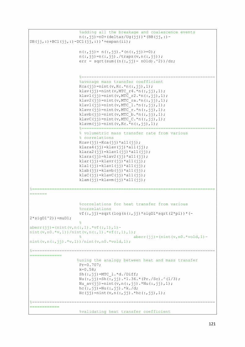
121

%adding all the breakage and coalescence events n(:,jj)=n0+(deltaz/Ug(jj))*(BB(jj,:)-

DB(jj,:)+BC1(jj,:)-DC1(jj,:))'+expan(ii);

n(:,jj)= n(:,jj).*(n(:,jj)>=0); n(:,jj)=n(:,jj)./trapz(v,n(:,jj)); err = sqrt(sum((n(:,jj)- nOld).^2))/dz;

%====================================================== %average mass transfer coefficient Kca(jj)=nint(v,Kc.*n(:,jj),1); klav(jj)=nint(v,MTC_r4.*n(:,jj),1); klav1(jj)=nint(v,MTC_r2.*n(:,jj),1); klav2(jj)=nint(v,MTC_ra.*n(:,jj),1); klavl(jj)=nint(v,MTC_l.*n(:,jj),1); klavr(jj)=nint(v,MTC_r.*n(:,jj),1); klavb(jj)=nint(v,MTC_b.*n(:,jj),1); klavC(jj)=nint(v,MTC_C.*n(:,jj),1); klavm(jj)=nint(v,Kc.*n(:,jj),1); %====================================================== % volumetric mass transfer rate from various % correlations Kcav(jj)=Kca(jj)*a11(jj); klara4(jj)=klav(jj)*a11(jj); klara2(jj)=klav1(jj)*a11(jj); klara(jj)=klav2(jj)*a11(jj); klar(jj)=klavr(jj)*a11(jj); klal(jj)=klavl(jj)*a11(jj); klab(jj)=klavb(jj)*a11(jj); klaC(jj)=klavC(jj)*a11(jj); klam(jj)=klavm(jj)*a11(jj);

%==========================================================================

=======

%correlations for heat transfer from various %correlations vf(:,jj)=sqrt(log(n(:,jj)*sigD1*sqrt(2*pi))*(-

2*sigD1^2))+muD1; %

aberr(jj)=(nint(v,n(:,1).*vf(:,1),1)-

nint(v,n0.*v,1))/nint(v,n(:,1).*vf(:,1),1); % aberr(jj)=(nint(v,n0.*vold,1)-

nint(v,n(:,jj).*v,1))/nint(v,n0.*vold,1);

%==========================================================================

============= %using the analogy between heat and mass transfer Pr=0.707; k=0.58; Sh(:,jj)=MTC_l.*d./Diff; Nu(:,jj)=Sh(:,jj).*1.36.*(Pr./Sc).^(1/3); Nu_av(jj)=nint(v,n(:,jj).*Nu(:,jj),1); hc(:,jj)=Nu(:,jj).*k./d; Hc(jj)=nint(v,n(:,jj).*hc(:,jj),1);

%==========================================================================

============ %validating heat transfer coefficient

122

Nu_w(:,jj)=2+(0.4*sqrt(Re1)+0.06*Re1.^(2/3))*Pr^0.4; Nu_wav(jj)=nint(v,n(:,jj).*Nu_w(:,jj),1);

Nu_c(:,jj)=1+0.752*((1+1./(Re1.*Pr)).^(1/3)).*Re1.^0.472.*Pr^(1/3); Nu_cav(jj)=nint(v,n(:,jj).*Nu_c(:,jj),1); else

%==========================================================================

============== %correlations for mass transfer coefficient % in each correlation, the mass transfer coefficient % and mass transfer rate are calculated % Ranz Sh_r=2+0.6*sqrt(Re1).*Sc.^(1/3); MTC_ra=Sh_r.*Diff./(2.*bradius); cAbra=t.*MTC_ra.*ap(ii).*MTC_ra./(1+t.*MTC_ra.*ap(ii)); ntotra(:,jj)=MTC_ra(ii).*ap(ii).*(cAs-cAbra(ii))'; % % Ranz2 Sh_ri=2+(1+0.273*Re1.^(0.5).*Sc.^(0.276)); MTC_r2=Sh_ri.*Diff./(2.*bradius); cAbr2=t.*MTC_r2.*ap(ii).*MTC_r2./(1+t.*MTC_r2.*ap(ii)); ntotr2(:,jj)=MTC_r2(ii).*ap(ii).*(cAs-cAbr2(ii))'; % Ranz4 Sh_re=2+0.6.*sqrt(Re1).*Sc.^(-1/6); MTC_r4=Sh_re.*Diff./(2.*bradius); cAbr4=t.*MTC_r4.*ap(ii).*MTC_r4./(1+t.*MTC_r4.*ap(ii)); ntotr4(:,jj)=MTC_r4(ii).*ap(ii).*(cAs-cAbr4(ii))'; % Linton Sh_fa=0.582.*(Re1.^0.5).*Sc.^(1/3); MTC_l=Sh_fa.*Diff./(2.*bradius); cAbl=t.*MTC_l.*ap(ii).*MTC_l./(1+t.*MTC_l.*ap(ii)); ntotl(:,jj)=MTC_l(ii).*ap(ii).*(cAs-cAbl(ii))'; % Rowel Sh_rl=2+0.68.*sqrt(Re1).*Sc.^(1/3); MTC_r=Sh_rl.*Diff./(2.*bradius); cAbr=t.*MTC_r.*ap(ii).*MTC_r./(1+t.*MTC_r.*ap(ii)); ntotr(:,jj)=MTC_r(ii).*ap(ii).*(cAs-cAbr(ii))'; % Brain Sh_b=(4+1.21.*((Re1.*Sc).^(0.67)).^0.5); MTC_b=Sh_b.*Diff./(2.*bradius); cAbb=t.*MTC_b.*ap(ii).*MTC_b./(1+t.*MTC_b.*ap(ii)); ntotb(:,jj)=MTC_b(ii).*ap(ii).*(cAs-cAbb(ii))'; % Clift Sh_c=((1+(1+(Re1.*Sc)).^(1/3))); MTC_C=Sh_c.*Diff./(2.*bradius); cAbC=t.*MTC_C.*ap(ii).*MTC_C./(1+t.*MTC_C.*ap(ii)); ntotC(:,jj)=MTC_C(ii).*ap(ii).*(cAs-cAbC(ii))';

%======================================================================== %the expansion term due mass transfer to the liquid %phase expan(ii)= nt(ii).*n(ii)+nt(ii).*v(ii).*((n(ii)-n(ii-

1))./(v(ii)-v(ii-1)));

%=================================================================== %mass transfer calculations cAb=t.*MTC_r4.*ap(ii).*cAs./(1+t.*MTC_C.*ap(ii)); cAbav(jj)=nint(v,cAb.*n(:,jj),1); ntot(:,jj)=MTC_r4(ii).*ap(ii).*(cAs-cAb(ii))'; nt(ii)=ntot(ii).*28.84/(epsG(jj)*rhoG); vloss(:,ii)=ntot(ii)*28.84./rhoG;

123

%=================================================================

%==========================================================================

===== %adding all the breakage and coalescence events n(:,jj)=n(:,jj-1)+(deltaz/Ug(jj))*(BB(jj,:)-

DB(jj,:)+BC1(jj,:)-DC1(jj,:))'+expan(ii);

n(:,jj)= n(:,jj).*(n(:,jj)>=0); n(:,jj)=n(:,jj)./trapz(v,n(:,jj)); err = sqrt(sum((n(:,jj)- nOld).^2))/dz;

%==========================================================================

======= %average mass transfer coefficient from various %correlations Kca(jj)=nint(v,Kc.*n(:,jj),1); klav(jj)=nint(v,MTC_r4.*n(:,jj),1); klav1(jj)=nint(v,MTC_r2.*n(:,jj),1); klav2(jj)=nint(v,MTC_ra.*n(:,jj),1); klavl(jj)=nint(v,MTC_l.*n(:,jj),1); klavr(jj)=nint(v,MTC_r.*n(:,jj),1); klavb(jj)=nint(v,MTC_b.*n(:,jj),1); klavC(jj)=nint(v,MTC_C.*n(:,jj),1); klavm(jj)=nint(v,Kc.*n(:,jj),1); %======================================================

% volumetric mass transfer rate from various % correlations Kcav(jj)=Kca(jj)*a11(jj); klara4(jj)=klav(jj)*a11(jj); klara2(jj)=klav1(jj)*a11(jj); klara(jj)=klav2(jj)*a11(jj); klar(jj)=klavr(jj)*a11(jj); klal(jj)=klavl(jj)*a11(jj); klab(jj)=klavb(jj)*a11(jj); klaC(jj)=klavC(jj)*a11(jj); klam(jj)=klavm(jj)*a11(jj);

vf(:,jj)=sqrt(log(n(:,jj)*sigD1*sqrt(2*pi))*(-

2*sigD1^2))+muD1; nint(v,n(:,jj).*v,1))/nint(v,n0.*vold,1);

%=============================================================== %using the analogy between heat and mass transfer Sh(:,jj)=MTC_l.*d./Diff; Nu(:,jj)=Sh(:,jj).*1.36.*(Pr./Sc).^(1/3); Nu_av(jj)=nint(v,n(:,jj).*Nu(:,jj),1); hc(:,jj)=Nu(:,jj).*k./d; Hc(jj)=nint(v,n(:,jj).*hc(:,jj),1);

%================================================================= %validating heat transfer coefficient Nu_w(:,jj)=2+(0.4*sqrt(Re1)+0.06*Re1.^(2/3))*Pr^0.4; Nu_wav(jj)=nint(v,n(:,jj).*Nu_w(:,jj),1);

Nu_c(:,jj)=1+0.752*((1+1./(Re1.*Pr)).^(1/3)).*Re1.^0.472.*Pr^(1/3); Nu_cav(jj)=nint(v,n(:,jj).*Nu_c(:,jj),1);

124

end; end end end vnew=v-vloss(jj,:)'; vcur(:,jj)=vnew; v=vnew; end

%==========================================================================

================================ % checking the volume balance and calculating total mass transfer rate

from the correlations for kk=1:Nc Ntot(kk)=nint(vcur(:,kk),n(:,kk).*ntot(:,kk).*Nb(kk),1); Ntotra(kk)=nint(vcur(:,kk),n(:,kk).*ntotra(:,kk).*Nb(kk),1); Ntotr2(kk)=nint(vcur(:,kk),n(:,kk).*ntotr2(:,kk).*Nb(kk),1); Ntotr4(kk)=nint(vcur(:,kk),n(:,kk).*ntotr4(:,kk).*Nb(kk),1); Ntotl(kk)=nint(vcur(:,kk),n(:,kk).*ntotl(:,kk).*Nb(kk),1); Ntotr(kk)=nint(vcur(:,kk),n(:,kk).*ntotr(:,kk).*Nb(kk),1); Ntotb(kk)=nint(vcur(:,kk),n(:,kk).*ntotb(:,kk).*Nb(kk),1); NtotC(kk)=nint(vcur(:,kk),n(:,kk).*ntotC(:,kk).*Nb(kk),1); if(kk==1) aberr(kk)=(nint(v,n0.*vold,1)-

nint(v,n(:,kk).*vcur(:,kk),1))/nint(v,n0.*vold,1); else aberr(kk)=(nint(v,Nb(kk-1).*n(:,kk-1).*vcur(:,kk-1),1)-

nint(v,Nb(kk).*n(:,kk).*vcur(:,kk),1))/nint(v,Nb(kk-1).*n(:,kk-

1).*vcur(:,kk-1),1); end end %==========================================================================

======================= %correlations for predicting gas hold-up in bubble columns epsGc=Ug./(0.3+2*Ug); epsGc1=0.91.*Ug.^1.19./(sqrt(g*dbs)); %Zahradnik et.al (1995) epsGc2=0.87*vgas1.^0.62; %Kelkar el.al(1983) epsGc3=0.475*vgas1.^0.37; %%Reilly et al. (1994) epsGc4=2.84.*vgas1.*rhoG^0.04./sigma^0.12; %%Reilly et al. (1986),(den, air density), (rawc, water density) epsGc5=(296.*vgas1.^0.44.*sigma^-0.16.*rhoL^-0.98.*rhoG^0.19)+0.009; %Joshi and Sharma epsGc6=vgas1./(0.3+2.*vgas1); %Hughmark epsGc7=1./(2+(0.35./vgas1)*(rhoL*sigma/72)^(1/3));

klac=0.0269*Ug.^0.82; klac1=Dc^0.17*Ug.^0.7; a11c=34.4.*Ug.^0.25.*epsG; a11c1=8.54*Ug.^0.12.*epsG; %==========================================================================

= %validating interfacial area A01=1030.*epsG.^0.87.*Ug.^0.2; A11=(6./sqrt(6.25))*(sigma/(rhoL*g))^-

0.5*(mew*Ug./sigma).^(1/4).*(rhoL.*sigma./(g*mew^4)).^(1/8).*epsG; nc=linspace(1,4,Nc); %=====graphical output=====================================================

125

figure; plot(nc,epsG,'-*',nc,epsGc,'-o',nc,epsGc1,'-s',nc,epsGc2,'-*',nc,epsGc3,'-

o',nc,epsGc4,'-s',nc,epsGc5,'-*',nc,epsGc6,'-o',nc,epsGc7,'-s') xlabel('column height (m)') ylabel('gas hold-up') legend('model','winkler','Joshi and Sharma','Zahradnik

','Kelkar','Reilly(1994)','Reilly(1986)','Joshi and Sharma','Hughmark') figure; plot(nc,a11,'-*') xlabel('column height (m)') ylabel('interfacial area (m^3/m^2)') figure; plot(nc,dbs,'-*') xlabel('column height (m)') ylabel('mean diameter (m)') figure; plot(nc,epsG,'-*') xlabel('column height (m)') ylabel('gas hold-up')

figure; plot(v,DC1,'-*',v,BC1,'-o') legend('death by coalescence', 'birth by coalescence') xlabel('bubble volume m^3') ylabel('sum of coalescence rates (1/m^3s)')

figure; plot(v,(BB),'-*',v,(DB),'-o') legend('birth by breakage','death by breakage') xlabel('bubble volume m^3') ylabel('sum of breakage rates(1/m^3s))')

figure; plot(v,n0,'-o', v, n,'-*') xlabel('bubble volume m^3') ylabel('number density') legend('initial size', '1^s^t compartment','2^n^d compartment','3^r^d

compartment','4^t^h compartment')

figure; plot(v,n0,'-o', v, n(:,1),'-*',v, n(:,4),'-sr') xlabel('bubble volume m^3') ylabel('number density') legend('initial size', '1^s^t compartment','4^t^h compartment')

figure; plot(vcur(:,1),hc(:,1),'-o') xlabel('bubble volume(m^3)') ylabel('heat transfer coefficient(W/m^2.K)')

126

Appendix B: Derivation of the heat transfer coefficient equation

Heat-transfer rate between the surface and the fluid is written as follows;

(C.1)

At the surface, heat transfer is by conduction and is expressed as follows:

(

) (C.2)

Equations (C.1) and (C.2) are equal

(

) (C.3)

Rearranging (C.3) results in

(C.4)

Since the thermal boundary layer can be written as

(C.5)

Equation (C.5) can be rearranged and written as

(C.6)