numerical method of neurostructural models training...
TRANSCRIPT

NUMERICAL METHOD OFNEUROSTRUCTURAL MODELS TRAININGBASED ON DECOMPOSITION OF WEIGHTS
AND PSEUDO-INVERSION
Pavel Saraev
Lipetsk State Technical University
Zvenigorod, Jun. 17-24, 2012

INTRODUCTION
Neuron-like element (NLE)
fNLE is a differentiable with respect to its arguments function
σ : X ×W → Y ,X ∈ Rn,W ∈ Rm,Y ∈ R,
where X is input space, W is weight space, Y is output space.
Neurostructural model (NSM)
NSM is a set of connected NLEs.
y = W (m)σ(m−1)(. . . σ(2)
(W (2), σ(1)
(W (1), x
)). . .)
= ψT (v)u,
where m is number of layers; σ(l) is a NLE transfer function of l-th layer;W (l) ∈ RNl×Nl−1 are weights between NLE of (l − 1)-th and l-th layers; uand v are linear and nonlinear weight vectors accordingly, ψ(v) = y (m−1).NSM has superpositional linear-nonlinear with respect to weights structure.
2/ 19

TYPICAL NSM
Figure. Feed-forward neural network
y = W (m)σ(m−1)(. . . σ(2)
(W (2)σ(1)
(W (1)x
)). . .)
3/ 19

SUBCLASSES OF NSM
NSM includes:
feed-forward neural networks (NN) (also with non-classic transfer func-tions);
radial basis functions (RBF)-NN;
probabilistic NN;
nonlinear Volterra NN;
Fahlman cascade-correlation NN;
Takagi-Sugeno fuzzy models with differentiable operators;
adaptive neuro-fuzzy implication systems (ANFIS).
4/ 19

NSM Training
Training problem
Given training set{xi , yi}, i = 1, . . . , k ,
where xi ∈ Rn is input vector of i-th example, yi ∈ Rr is real output vector.Training of one-output NSM (r = 1) is nonlinear least squares problem(NLSP):
w∗ = arg minw∈Rs
J(w),
J(w) = J(u, v) =k∑
i=1
(yi (w)− yi )2 = ‖y − y‖22, (1)
where y and y are model and real output vectors accordingly.
5/ 19
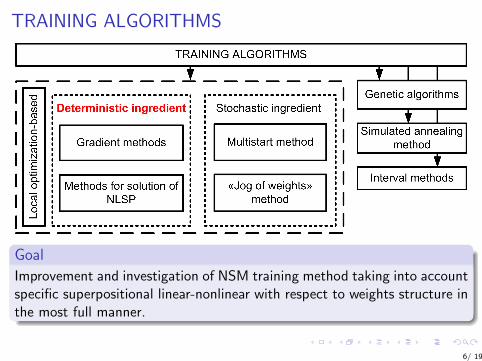
TRAINING ALGORITHMS
Goal
Improvement and investigation of NSM training method taking into accountspecific superpositional linear-nonlinear with respect to weights structure inthe most full manner.
6/ 19
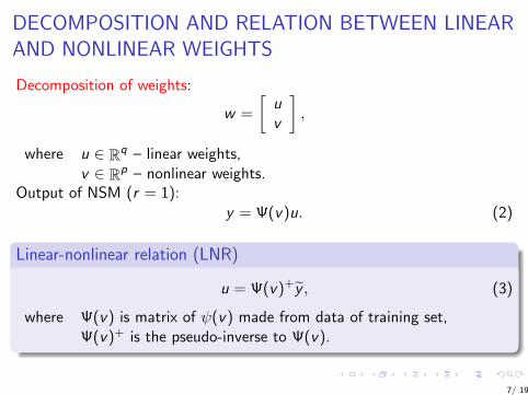
DECOMPOSITION AND RELATION BETWEEN LINEARAND NONLINEAR WEIGHTS
Decomposition of weights:
w =
[uv
],
where u ∈ Rq – linear weights,v ∈ Rp – nonlinear weights.
Output of NSM (r = 1):y = Ψ(v)u. (2)
Linear-nonlinear relation (LNR)
u = Ψ(v)+y , (3)
where Ψ(v) is matrix of ψ(v) made from data of training set,Ψ(v)+ is the pseudo-inverse to Ψ(v).
7/ 19
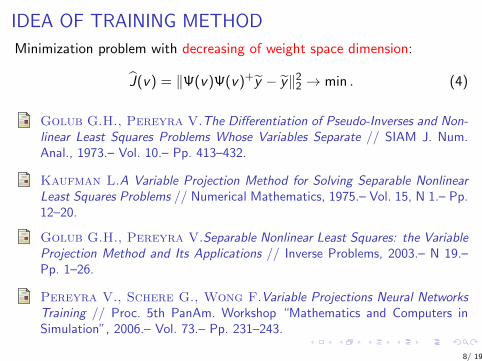
IDEA OF TRAINING METHOD
Minimization problem with decreasing of weight space dimension:
J(v) = ‖Ψ(v)Ψ(v)+y − y‖22 → min . (4)
Golub G.H., Pereyra V.The Differentiation of Pseudo-Inverses and Non-linear Least Squares Problems Whose Variables Separate // SIAM J. Num.Anal., 1973.– Vol. 10.– Pp. 413–432.
Kaufman L.A Variable Projection Method for Solving Separable NonlinearLeast Squares Problems // Numerical Mathematics, 1975.– Vol. 15, N 1.– Pp.12–20.
Golub G.H., Pereyra V.Separable Nonlinear Least Squares: the VariableProjection Method and Its Applications // Inverse Problems, 2003.– N 19.–Pp. 1–26.
Pereyra V., Schere G., Wong F.Variable Projections Neural NetworksTraining // Proc. 5th PanAm. Workshop “Mathematics and Computers inSimulation”, 2006.– Vol. 73.– Pp. 231–243.
8/ 19
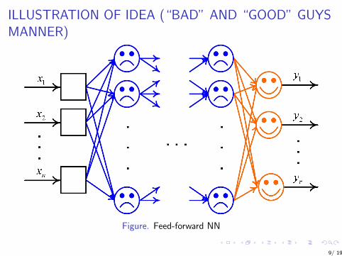
ILLUSTRATION OF IDEA (“BAD” AND “GOOD” GUYSMANNER)
Figure. Feed-forward NN
9/ 19

PROPOSED APPROACH
Usage of usual 2-dimensional matrices for derivatives instead of3-dimensional and without any decomposition of Ψ.
10/ 19
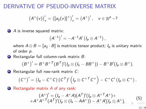
DERIVATIVE OF PSEUDO-INVERSE MATRIX(A+(v)
)′v
=([aij(v)]+
)′v
=(A+)′, v ∈ Rp −?
1 A is inverse squared matrix:(A−1
)′= −A−1A′
(Ip ⊗ A−1
),
where A⊗B = [aij · B] is matrices tensor product; Ip is unitary matrixof order p.
2 Rectangular full column-rank matrix B:(B+)′
= B+B+T (BT )′(Ip ⊗ (Ik − BB+))− B+B ′(Ip ⊗ B+).
3 Rectangular full row-rank matrix C :(C+)′
=(Iq − C+C
)(CT )′
(Ip ⊗ C+TC+
)− C+C ′
(Ip ⊗ C+
).
4 Rectangular matrix A of any rank:
(A+)′
= (Iq − A+A)(AT )′(Ip ⊗ A+TA+)++A+A+T (AT )′(Ip ⊗ (Ik − AA+))− A+A′(Ip ⊗ A+).
(5)
11/ 19

ALGORITHMIC BASEResidual vector:
H(v) = Ψ(v)Ψ(v)+y − y = (Ψ(v)Ψ(v)+ − Ik)y ;(ΨΨ+
)′= Ψ+T (ΨT )′(Ip ⊗ (Ik −ΨΨ+)) + (Ik −ΨΨ+)Ψ′(Ip ⊗Ψ+). (6)
Derivative of H(v) (the Jacobi matrix):
H ′ = Ψ+T (ΨT )′(Ip ⊗ (Ik −ΨΨ+)y)++(Ik −ΨΨ+)Ψ′(Ip ⊗Ψ+y) ∈ Rk×p.
(7)
Gauss-Newton method
Gauss and Newton’s method for minimization of (4) with pseudo-inversion:
∆v = −[(R ′)TR ′
]+(R ′)TR; R ′ = L (Ip ⊗ y) ;
K = Ik −ΨΨ+; L = K Ψ′ (Ip ⊗Ψ+) + Ψ+T (ΨT )′ (Ip ⊗ K ) ,(8)
where ∆v is direction of minimization of nonlinear weight vector v .
12/ 19

MULTILAYER NSM CASE
Ψ′ =
[∂y
(m−1)i
∂w(h,k)j
]– ?
Superpositional structure of NSM is used:
∂y(m−1)i
∂w(h,k)j
=∂y
(m−1)i
∂yhk
∂yhk
∂net(h,k)j
∂net(h,k)j
∂w(h,k)j
,
where w(h,k)j is j-th weight of k-th NLE of h-th layer.
s(i ,h,k) =∂y
(m−1)i
∂yhk
=
Nh+1∑l=1
s(i ,h+1,l)∂y(h+1)l
∂yhk
, h = m − 2, . . . , 1;
Initial value:
s(i ,m−1,l) =∂y
(m−1)i
∂y(m−1)l
=
{1, i = j0, i 6= j
, i , j = 1, . . . ,Nm−1.
13/ 19

MULTIOUTPUT NSM CASE
U ∈ Rq×r are last hidden NLE’s weights
Y = Ψ(v)U
‖H(v)‖2F = ‖Ψ(v)Ψ(v)+Y − Y ‖2F = ‖ vecH(v)‖2 =
= ‖ vec(
Ψ(v)Ψ(v)+Y)− vec Y ‖2,
where vec is the operation of matrix vectorization, Y ∈ Rk×r is the matrixof real outputs.
(vecH(v))′ =(
Ir ⊗(Ψ(v)Ψ(v)+
)′)
Ip ⊗ y1Ip ⊗ y2. . .
Ip ⊗ yr
∈ Rkr×p, (9)
where (Ψ(v)Ψ(v)+)′
is determined by (6).
14/ 19

EXPERIMENTS: quality of minimization400 randomly generated tested problems
Figure. Pairwise comparison by quality15/ 19
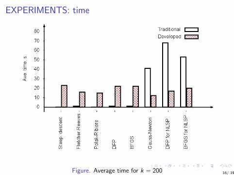
EXPERIMENTS: time
Figure. Average time for k = 200 16/ 19
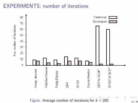
EXPERIMENTS: number of iterations
Figure. Average number of iterations for k = 200 17/ 19

CONCLUSION
Results
Class of NSM is introduced.
Optimizing weight space dimension is decreased.
Formula for derivative of pseudo-inverse matrix is developed.
Algorithmic base for minimization of modified function is developed.
Algorithm for last hidden NLE’s outputs is suggested.
Software for numerical experiments is developed.
Numerical experiments were conducted.
The developed numerical method is highly recommended for trainingsets of small sizes (less than 60).
18/ 19
