NUMERICAL METHODS FOR DIFFUSION THEORY CRITICALITY © M. Ragheb 4/11/2008 1. INTRODUCTION

The diffusion equation can be solved analytically for simple geometries and material compositions such as homogeneous reactors. More complex reactor designs involve multiple regions of different compositions such as core regions with fissile materials and reflector regions with scattering materials. This suggests the discretization of the diffusion equation in the spatial variable at specified mesh points and the use of computers to solve the ensuing linear system of equations for the magnitude of the flux at 4each mesh point, as well as the corresponding eigen-value which is the effective multiplication factor. 2. THE ONE GROUP DIFFUSION EQUATION Multi-group diffusion theory problems involve a calculation in the spatial variable for each group of neutrons. To study the treatment of the spatial variable, we thus concentrate on the treatment of the one-group diffusion equation:

)()()()()]()(.[ rrk

rrrrD ff

a φν

φφ Σ=Σ+∇∇− (1)

where we explicitly account for the spatial dependence of the diffusion coefficient D, the macroscopic absorption cross section )(raΣ , the macroscopic fission cross section

)(rfΣ , and the neutron flux )(rφ . The factor k is here the eigen-value belonging to the fundamental eigen-vector

)(rφ . If k > 1, the system is supercritical, since the neutron production must be reduced for the neutron balance to be valid. If k = 1, then the losses of neutrons are equal to the production rate and the system is critical. If k < 1, the system is subcritical. Thus k can be identified as the effective multiplication factor of the multiplying system. In addition to Eqn. 1, we must satisfy the boundary condition that the neutron flux vanishes at the extrapolated boundary of the system: ( ) ( 0.71 ) ( ) 0tr eR d R Rφ φ λ φ+ = + = = (2) where R is the reactor’s core radius in spherical geometry, and trλ is the transport mean free path.

1

3. ANALYTICAL EXPRESSION FOR THE MULTIPLICATION FACTOR In spherical geometry Eqn. 1 becomes:

)()()()()]()([1 22 rr

krrr

drdrDr

drd

r ff

a φν

φφ Σ=Σ+− (3)

For a homogeneous reactor,

D(r) = D =constant, aΣ , fΣ = constant,

and Eqn. 3 simplifies to:

0)(][1])(2)(2

2

=Σ−Σ++ rkDdr

rdrdr

rdaf

f φνφφ (4)

If we let:

rrur )()( =φ (5)

thus: 2

)()(1)(rru

drrdu

rdrrd

−=φ

and: 322

2

22

2 )(2)(1)(1)(1)(rru

drrdu

rdrrud

rdrrdu

rdrrd

+−+−=φ

Substituting in Eqn. 4, we get:

0][12122112 3232

2

2 =Σ−Σ

+−+++−ru

kDru

drdu

rru

drrd

rdrdu

r affν

Upon cancellation of terms, we get:

012

2

=⎥⎦

⎤⎢⎣

⎡Σ−

Σ+ u

kDdrud

affν

(6)

Equation 6 has a solution: )sin()cos( BrCBrAu += (7)

2

From Eqn.5, the neutron flux is thus given by:

r

BrCr

BrA )sin()cos(+=φ (8)

where the material buckling is given by:

⎥⎦

⎤⎢⎣

⎡Σ−

Σ= a

ffm kD

Bν12 (9)

Since the neutron flux must remain finite at the center of the reactor’s core at r =

0, this implies that the constant A = 0, and:

r

BrC )sin(=φ (10)

At the extrapolated core boundary, Eqn. 2 applies, and we get:

0)sin(

)( ==e

ee R

BRCRφ (11)

where tre RR λ71.0+= is the extrapolated radius. This implies that: ,...3,2,1, == nnBRe π (12) For the fundamental mode eigenvalue, n = 1, and the geometrical buckling is given by:

22 )(e

g RB π

= (13)

The criticality condition is obtained by equating the geometrical buckling to the material buckling, to the buckling in general: 222 BBB mg == Thus using Eqns. 9 and 13 we get:

3

2)(1

ea

ff

RkDπν

=⎥⎦

⎤⎢⎣

⎡Σ−

Σ

from which we the criticality equation in spherical geometry as:

2)(

ea

ff

RD

kπ

ν

+Σ

Σ= (14)

Another form for the multiplication factor k can be obtained from Eqn. 1 if we integrate over the reactor’s volume:

∫ ∫

∫Σ+∇∇−

Σ=

V Va

Vff

dVrrdVrD

dVrrk

)()()](.[

)()(

φφ

φν (15)

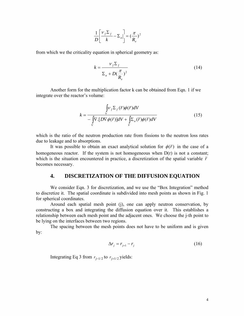
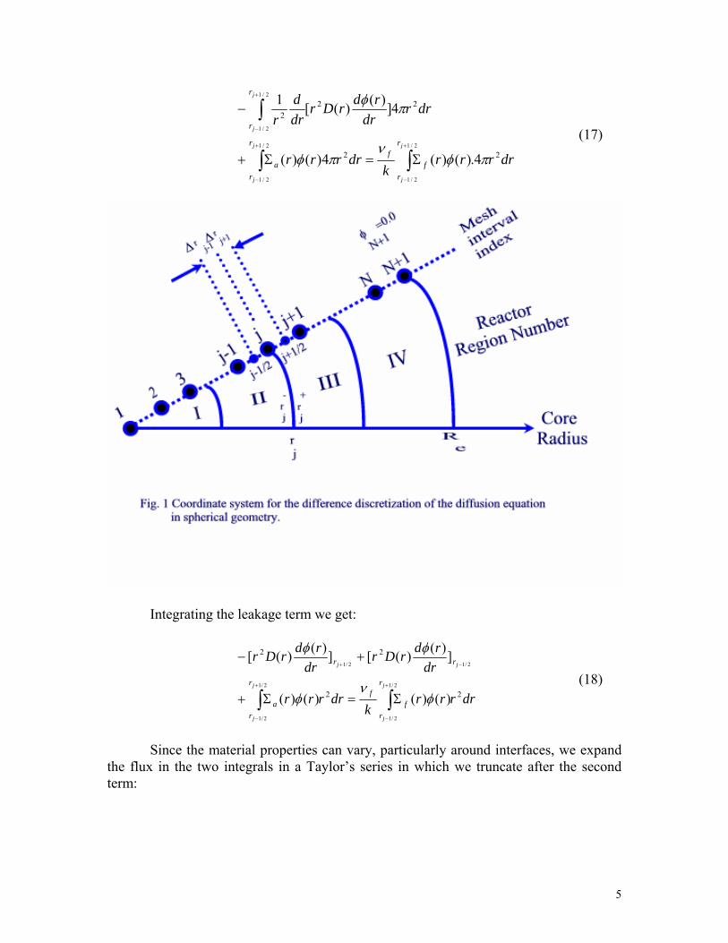
which is the ratio of the neutron production rate from fissions to the neutron loss rates due to leakage and to absorptions. It was possible to obtain an exact analytical solution for )(rφ in the case of a homogeneous reactor. If the system is not homogeneous when D(r) is not a constant; which is the situation encountered in practice, a discretization of the spatial variable r becomes necessary. 4. DISCRETIZATION OF THE DIFFUSION EQUATION We consider Eqn. 3 for discretization, and we use the “Box Integration” method to discretize it. The spatial coordinate is subdivided into mesh points as shown in Fig. 1 for spherical coordinates. Around each spatial mesh point (j), one can apply neutron conservation, by constructing a box and integrating the diffusion equation over it. This establishes a relationship between each mesh point and the adjacent ones. We choose the j-th point to be lying on the interfaces between two regions. The spacing between the mesh points does not have to be uniform and is given by: jjj rrr −=∆ +1 (16)

Integrating Eq 3 from to yields: 2/1−jr 2/1+jr

4

drrrrk

drrrr

drrdr

rdrDrdrd

rj

j

j

j

j

j

r

rf

fr

ra

r

r

22

222

4.)()(4)()(

4])()([1

2/1

2/1

2/1

2/1

2/1

2/1

πφν

πφ

πφ

∫∫

∫+

−

+

−

+

−

Σ=Σ+

−

(17)

Integrating the leakage term we get:

drrrr

kdrrrr

drrdrDr

drrdrDr

j

j

j

j

jj

r

rf

fr

ra

rr

22

22

2/1

2/1

2/1

2/1

2/12/1

)()()()(

])()([])()([

∫∫+

−

+

−

−+

Σ=Σ+

+−

φν

φ

φφ

(18)

Since the material properties can vary, particularly around interfaces, we expand

the flux in the two integrals in a Taylor’s series in which we truncate after the second term:

5

drdr

rdrrrrr

drdr

rdrrrrr

drrrrdrrrrdrrrrI

j

j

j

j

j

j

j

j

j

j

r

r j

jjjjjaj

r

r j

jjjjjaj

r

ra

r

ra

r

ra

∫

∫

∫∫∫

+

+

−

−

+

+

−

−

+

−

+−+Σ+

++−−Σ=

Σ+Σ=Σ=

++

++++

−

−−−−+

2/1

2/1

2/1

2/1

2/1

2/1

...])(

)()()[()(

...])(

)()()[()(

)()()()()()(

2/12

2/12

2221

φφ

φφ

φφφ

(19)

If we make the approximations:

222 )()()( jjj rrr ≅≅ +−

∫ ∫ −≅−

−

−

+

+

++

+

−

−−

j

j

j

j

r

r

r

r j

jjj

j

jjj dr

dr

rdrrdr

dr

rdrr

2/1

2/1 )()(

)()( 2/12/1

φφ

the integral is approximately equal to:

2)(

)()()(2

)()()()(

))(()()())(()()(

))(()()())(()()(

1212

2/12

2/12

2/12

2/12

1

jjjjaj

jjjjaj

jjjjajjjjjaj

jjjjajjjjjaj

rrrrr

rrrrr

rrrrrrrrrr

rrrrrrrrrrI

−Σ+

−Σ≅

−Σ+−Σ≅

−Σ+−Σ≅

++−−

++

−−

++

++−

−−−

φφ

φφ

φφ

(20)

where we used approximation:

)()()( jjj rrr φφφ ≅≅ +−

In the case where: )()( +− Σ≅Σ jaja rr , which applies to all the points except at the interfaces, we get: )()( +− Σ≅Σ jaja rr and:

6

2)()(

2)()(

12

1121

−

−+

∆+∆Σ≅

−Σ≅

jjjjaj

jjjjaj

rrrrr

rrrrrI

φ

φ (21)

The same relationship holds for the source integral:

2

.))(()( 122

−∆+∆Σ≅ jj

jjjff rr

rrrk

I φν

(22)

Substituting in Eq. 18 we can write:

2.))(()(

2)()(])()([])()([

12

12222/12/1

−

−

∆+∆Σ=

∆+∆Σ+−

+−

jjjjjf

f

jjjjajrr

rrrrr

k

rrrrr

drrdrDr

drrdrDr

jj

φν

φφφ

(23)

We can now approximate the derivatives by forward first order difference equations:

1

1)()()(

2/1 −

−

∆

−≅⎥⎦

⎤⎢⎣⎡

− j

jj

r rrr

drrd

j

φφφ (24)

1

1 )()()(

2/1 −

+

∆

−≅⎥⎦

⎤⎢⎣⎡

+ j

jj

r rrr

drrd

j

φφφ (25)

Inserting Eqns. 24 and 25 into Eqn. 21, we get:

2.))(()(

2)()(

)()(

)()(

)()(

)()(

12

12

12/1

22/12/1

22/1

1

12/1

22/1

12/1

22/1

−

−

+++++

−

−−−

−−−

∆+∆Σ=

∆+∆Σ

+∆

−∆

+∆

−∆

jjjjjf

f

jjjjaj

j

jjj

j

jjj

j

jjj

j

jjj

rrrrr

k

rrrrr

rr

rDrrr

rDr

rr

rDrrr

rDr

φν

φ

φφ

φφ

(26)

At an interface the last two terms are replaced by their equivalents from Eq.20 as:

7

2))(()(

2))(()(

2)()(

2)()(

)()(

)()(

)()(

)()(

212

212

12/1

22/12/1

22/1

1

12/1

22/1

12/1

22/1

jjjjf

fjjjjf

f

jjjaj

jjjaj

j

jjj

j

jjj

j

jjj

j

jjj

rrrr

k

rrrr

k

rrrr

rrrr

rr

rDrrr

rDr

rr

rDrrr

rDr

∆Σ+

∆Σ=

∆Σ+

∆Σ

+∆

−∆

+∆

−∆

+−−

+−−

+++++

−

−−−

−−−

φν

φν

φφ

φφ

φφ

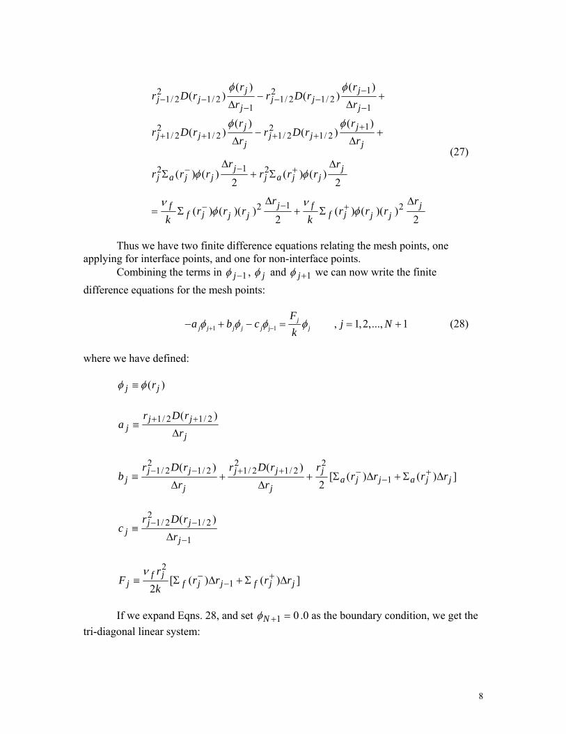
(27)

Thus we have two finite difference equations relating the mesh points, one

applying for interface points, and one for non-interface points. Combining the terms in 1−jφ , jφ and 1+jφ we can now write the finite

difference equations for the mesh points:

1 j 1 , 1,2,..., 1jj j j j j j

Fa b c j N

kφ φ φ φ+ −− + − = = + (28)

where we have defined:

)( jj rφφ ≡

j

jjj r

rDra

∆≡ ++ )( 2/12/1

])()([2

)()(1

22/1

22/12/1

22/1

jjajjaj

j

jj

j

jjj rrrr

rrrDr

rrDr

b ∆Σ+∆Σ+∆

+∆

≡ +−

−++−−

1

2/12

2/1 )(

−

−−

∆≡

j

jjj r

rDrc

])()([2 1

2

jjfjjfjf

j rrrrkr

F ∆Σ+∆Σ≡ +−

−ν

If we expand Eqns. 28, and set 01 =+Nφ .0 as the boundary condition, we get the

tri-diagonal linear system:

8

NN

NNNN kFbc

kFabckFabckFab

φφφ

φφφφ

φφφφ

φφφ

=+−

===

=−+−

=−+−

=−+

−1

33

433323

22

322212

11

2111

....

....

.... (29)

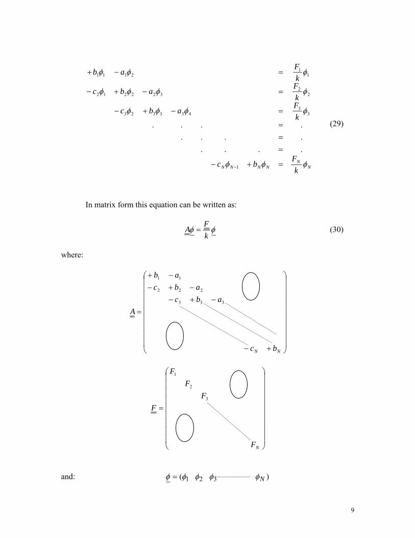
In matrix form this equation can be written as:

φφkF

A = (30)

where:

⎟⎟⎟⎟⎟⎟⎟⎟⎟

⎠

⎞

⎜⎜⎜⎜⎜⎜⎜⎜⎜

⎝

⎛

+−

−+−−+−

−+

=

NN bc

abcabc

ab

A333

222

11

⎟⎟⎟⎟⎟⎟⎟⎟⎟

⎠

⎞

⎜⎜⎜⎜⎜⎜⎜⎜⎜

⎝

⎛

=

NF

FF

F

F3

2

1

and: 1(φφ = 2φ 3φ )Nφ

9

The method used above is called a "three-point difference method" since the flux

equations at three neighboring points j-1, j and j+1 are coupled to each other. 5. TREATMENT OF DIFFERENT GEOMETRIES The previous derivation is formulated for spherical geometry. For other geometries, the leakage term is written in general as:

)]([1).(drdDr

drd

rD φφ γ

γ=∇∇ (31)

where:

0=γ , for cartesian coordinates 1=γ , for cylindrical coordinates 2=γ , for spherical coordinates

The volume elements in each case are also given by:

drrdV γδγγ

γπ )1( 02 −= (32) where:

00 =γδ , ∀ 0≠γ 1= , ∀ 0=γ ,

is the Kronecker delta.

The 2π or 4π factors do not appear in the finite difference equations. The volume element is a true volume element only in spherical coordinates. In cylindrical coordinates it is a surface element, and it is a line element in slab geometry. 6. THE BUCKLING CORRECTION FOR MULTIMENSIONAL SYSTEMS The buckling correction allows accounting for three-dimensional effects in a one-dimensional numerical calculation, by recognizing that the buckling in a given dimension represents neutron leakage and can be replaced by an effective absorption rate term. In three dimensions and cartesian coordinates, the diffusion equation:

0)()()( =Σ

+Σ−∂∂

∂∂

+∂∂

∂∂

+∂∂

∂∂ φ

νφφφφ

kzD

zyD

yxD

xff

a (33)

10

If we solve the equation in the x-direction only but wish to account for the neutron leakage in the y and z directions, assuming homogeneity in those directions, we can do this by writing:

022

22

2

=+=+ φφφφzy B

dzdB

dyd (34)

Thus Eqn. 33 can be written as:

[ ] 0)()()()( 22 =Σ

+Σ++−⎥⎦⎤

⎢⎣⎡ x

kxDBB

dxxdD

dxd ff

azy φν

φφ

or:

0)()()( ' =Σ

+Σ−⎥⎦⎤

⎢⎣⎡ x

kx

dxxdD

dxd ff

a φν

φφ (35)

where a modified macroscopic cross section term in cartesian coordinates is used as: [ ]azya DBB Σ++=Σ )( 22' (36)

In cylindrical coordinates, it becomes: [ ]aza DB Σ+=Σ 2' (37)

Thus one can compensate for the leakages that are not included in a one-dimensional calculation by assuming homogeneity in the untreated directions. 7. CRITICALITY OF BARE UNREFLECTED REACTOR CORES We consider a bare unreflected spherical reactor core with the following parameters:

Radius R = 50.0 [cm] Diffusion coefficient D = 1.0 [cm] Macroscopic absorption cross section: ∑

a = 0.75 [cm

-1]

Product of macroscopic fission cross section and neutron yield per fission: ν∑

f = 0.78 [neutron.cm

-1]

The diffusion area of the reactor can be calculated as:

2 21 1.333[ ]0.75a

DL c= = =Σ

m

11

The geometric buckling is:

2 2 2

2 33.948 10 [ ]50b

e

2B x cmR Rπ π π − −⎛ ⎞ ⎛ ⎞ ⎛ ⎞= ≈ = =⎜ ⎟ ⎜ ⎟ ⎜ ⎟

⎝ ⎠ ⎝ ⎠⎝ ⎠

where we are ignoring the extrapolated distance.

We rewrite Eqn. 14 as:

2 22 2 1( ) 1 ( )

f f

f f a

ae a e

kk D L BDR R

νν

π π∞

ΣΣ Σ

= = =+Σ + +

Σ

(38)

We can then calculate the infinite medium multiplication factor from Eqn. 38 as:

0.78 1.040.75

f

a

kν

∞

Σ= = =

Σ

and consequently an exact analytical solution for the effective multiplication factor can be calculated as:

2 2 3

1.04 1.034551 1 1.333 3.948 10eff

g

kkL B x x∞

−= = =+ +

If the numerical code is used to calculate this value of the effective multiplication

factor, the following input data file for a single “1” region reactor, a spherical geometry “2”, and a convergence factor of “0.1e-5”, and the values of the radius (R = 50.0 [cm]), diffusion coefficient (D = 1.0 [cm]), macroscopic absorption cross section (∑

a = 0.75

[cm-1

]), and the product of the average number of neutron per fission and macroscopic fission cross section (ν∑

f = 0.78 [neutron.cm

-1]), and zero geometric buckling correction

values, can be used as input values: 1 2+0.1e-05 50.0 1.0 0.75 0.78 0.000 0.000 0.000

The numerical value for the effective multiplication value is remarkably similar to the earlier obtained analytical value as:

12

( ) 1.0345eff numericalk =

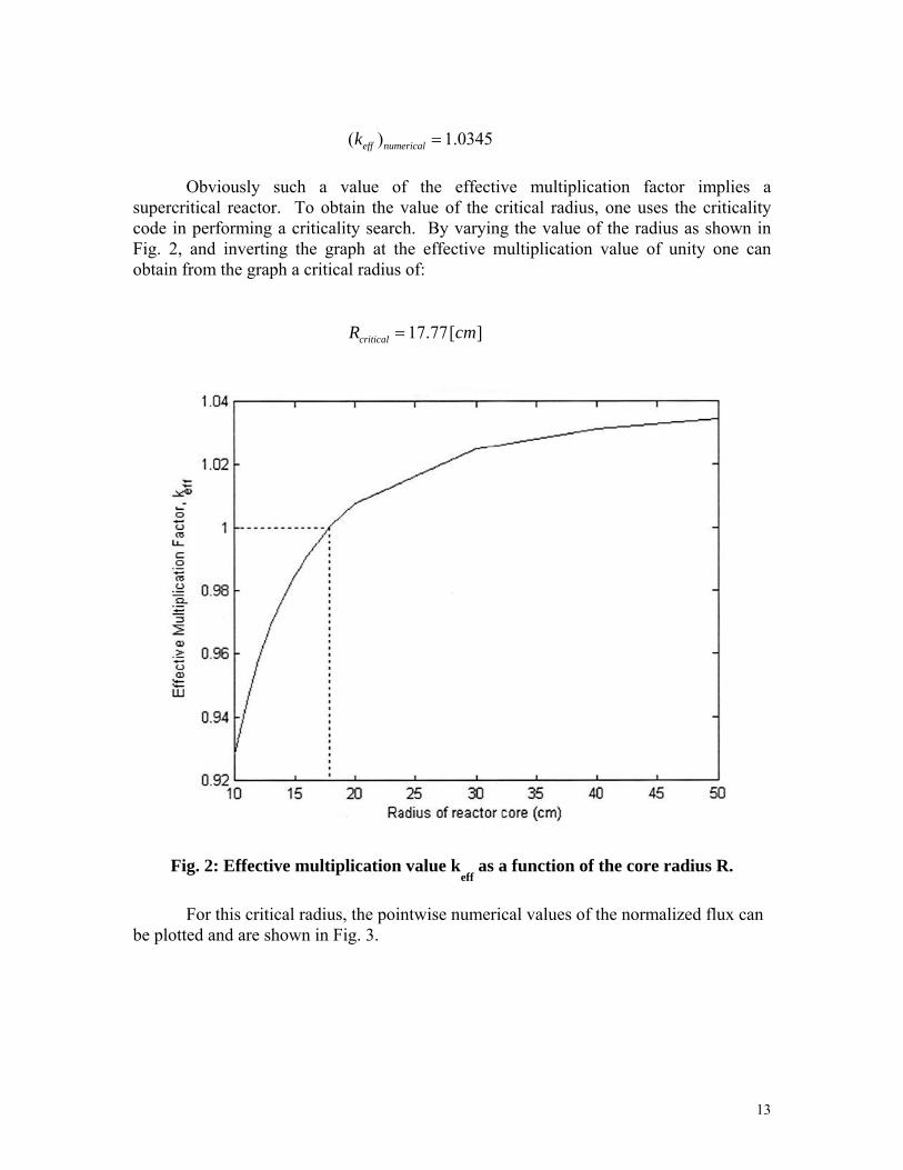
Obviously such a value of the effective multiplication factor implies a supercritical reactor. To obtain the value of the critical radius, one uses the criticality code in performing a criticality search. By varying the value of the radius as shown in Fig. 2, and inverting the graph at the effective multiplication value of unity one can obtain from the graph a critical radius of: 17.77[ ]criticalR cm=

Fig. 2: Effective multiplication value keff

as a function of the core radius R.

For this critical radius, the pointwise numerical values of the normalized flux can be plotted and are shown in Fig. 3.

13

Fig. 3: Normalized flux distribution for the critical core. 8. CRITICALITY OF REFLECTED CORES

The advantage of a numerical approach to criticality becomes apparent when one deals with geometries and configurations that do not easily lend themselves to the derivation of exact analytical solutions like in the previous case. To demonstrate the usefulness of the numerical approach, we consider here the criticality of a reflected core. In this situation, the reactor geometry consists of two regions. The core region contains a fissile material and is a multiplying medium in nature, and the outer region is a scattering material.

This type of problem contains two degrees of freedom. By varying both the reflector thickness and the inner core radius, one in fact obtains a three dimensional surface of the effective multiplication factor as a function of the core radius and the reflector thickness. The critical configuration is obtained as the intersection of this surface with the plane representing an effective multiplication factor equal to unity. This intersection can be projected on the plane of the core radius and reflector thickness leading to a curve describing the combination of core radius and reflector thickness that would make the system critical.

14

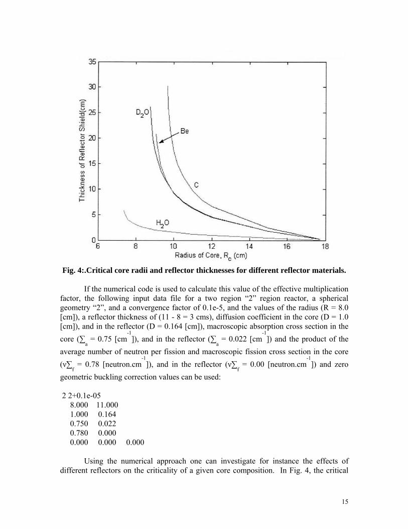
Fig. 4:.Critical core radii and reflector thicknesses for different reflector materials.

If the numerical code is used to calculate this value of the effective multiplication

factor, the following input data file for a two region “2” region reactor, a spherical geometry “2”, and a convergence factor of 0.1e-5, and the values of the radius (R = 8.0 [cm]), a reflector thickness of (11 - 8 = 3 cms), diffusion coefficient in the core (D = 1.0 [cm]), and in the reflector (D = 0.164 [cm]), macroscopic absorption cross section in the core (∑

a = 0.75 [cm

-1]), and in the reflector (∑

a = 0.022 [cm

-1]) and the product of the

average number of neutron per fission and macroscopic fission cross section in the core (ν∑

f = 0.78 [neutron.cm

-1]), and in the reflector (ν∑

f = 0.00 [neutron.cm

-1]) and zero

geometric buckling correction values can be used: 2 2+0.1e-05 8.000 11.000 1.000 0.164 0.750 0.022 0.780 0.000 0.000 0.000 0.000

Using the numerical approach one can investigate for instance the effects of different reflectors on the criticality of a given core composition. In Fig. 4, the critical

15

core radius and the associated reflector thicknesses using different moderators is shown. It can be noticed that the reflector leads to a smaller critical radius in all the choices of reflector materials, than the unreflected bare core.

If light water is chosen as the reflector material, Fig. 5 shows a choice of a critical core radius at 8 cms, and an associated 3 cms of a water reflector. This is much smaller than the critical radius of the bare core at 17.7 cms. Figure 5 shows the normalized core and reflector flux distribution for light water as a reflector.

Fig. 5: A choice of a critical core radius and an associated reflector thickness for light water as a reflecting material.

16

Fig. 6: Normalized core and reflector flux distribution for light water as a reflector.

EXERCISES 1. Calculate analytically the effective multiplication factor for a one region one dimensional spherical reactor core with the following parameters, then compare the results to those calculated numerically with the criticality code listed in the Appendices. Radius R = 50.0 cm Diffusion coefficient D = 1.0 cm Macroscopic absorption cross section: ∑a = 0.75 cm-1

Product of macroscopic fission cross section and neutron yield per fission: ν∑f = 0.78 neutron.cm-1

2. Consider a spherical reactor core with the following parameters: R = 35 [cms] D = 1.0 [cm]

aΣ = 0.75 [cm-1

]

fνΣ =0.78 [neutron.cm-1

] 1p fε = = ≈

a) Use the one-group diffusion theory to calculate the infinite medium multiplication factor, the diffusion area, the geometric buckling, and the effective multiplication factor. b) Calculate analytically the radius that will make this reactor just critical.

17

c) Now use the numerical criticality code to check the analytical result for the effective multiplication factor, and compare it to the analytical result given in part1 above. Plot the normalized flux distribution. d) Perform a “Criticality Search” by varying the radius of the reactor, plot the value of the effective multiplication factor against the radius, and deduce the critical radius, or the radius that will make the effective multiplication factor equal to unity. Check the numerical result against the analytical result in part 2 above. e) Now, surround your reactor with a reflector of your choice (e.g. H

2O, D

2O, Be, C,

U238

, etc.). Treat the problem as a two-region reactor. By varying both the thickness of the reflector and the radius of the core, optimize the design by determining a choice of appropriate core radius and reflector thickness. Justify your choice of the optimal configuration. Plot your results and discuss your observations and findings. Plot the normalized flux in your optimized final configuration. REFERENCES

1. M. Ragheb, “Lecture Notes on Fission Reactors Design Theory,” FSL-33, University of Illinois, 1982.

2. J. R. Lamarsh, “Introduction to Nuclear Engineering,” Addison-Wesley Publishing Company, 1983. APPENDIX

CRITICALITY CODE LISTING !!!!!!!!!!!!!!!!!!!!!!!!!!!!!!!!!!!!!!!!!!!!!!!!!!!!!!!!!!!!!!!!!!!!!!!!!!!!!!!!!!!!!!!!!!!! ! Multiregion One-dimensional One-group Diffusion Theory Criticality Code ! Evaluation of Effective Multiplication Factor or Eigenvalue and Normalized Neutron Flux ! Enhanced version of the ODOG procedure using the Power Iteration Method ! ANSI Fortran-90 or 95 procedure. Unix or Windows operating System. !!!!!!!!!!!!!!!!!!!!!!!!!!!!!!!!!!!!!!!!!!!!!!!!!!!!!!!!!!!!!!!!!!!!!!!!!!!!!!!!!!!!!!!!!!!! ! Dr. M. Ragheb ! Department of Nuclear, Plasma and Radiological Engineering ! University of Illinois at Urbana-Champaign ! 216 Talbot Laboratory, 104 S. Wright St., Urbana, Illinois 61801, USA. !!!!!!!!!!!!!!!!!!!!!!!!!!!!!!!!!!!!!!!!!!!!!!!!!!!!!!!!!!!!!!!!!!!!!!!!!!!!!!!!!!!!!!!!!!!! program criticality ! ! Version 4.5, 2008 !!!!!!!!!!!!!!!!!!!!!!!!!!!!!!!!!!!!!!!!!!!!!!!!!!!!!!!!!!!!!!!!!!!!!!!!!!!!!!!!!!!!!!!!!!!! real lamda1,lamda2 ! lamda1 = first eigenvalue iteration ! lamda2 = second eigenvalue iteration ! Maximum number of regions in dimension statement = 5 dimension rr(5),delx(5),n(5),r(100),rp12(100),rm12(100),delr(100) ! rr = distances delimiting regions, measured from plane of symmetry [cm] ! delx = size of interval in each region, chosen as equal to or less than the neutron ! mean free path in the region [cm] ! n = number of intervals in each region ! r = r(j) = distance of each point from the origin ! rp12 = r(j + 1/2)

18

! rm12 = r(j - 1/2) ! delr = r(j+1)-r(j) dimension d(5),dp12(100),dm12(100),sigma(5),sigp(100),sigm(100) ! d = diffusion coefficient in each region [cm] ! dp12 = d(j + 1/2) ! dm12 = d(j - 1/2) ! sigma = macroscopic absorption cross section in each region [cm-1] ! sigp = sigma(j+) ! sigm = sigma(j-) dimension ms(5),f(5),fp(100),fm(100),a(100),b(100),c(100),w(100),biga(100,100) ! ms = number of intervals up to and including each region ! f = nu*sigmaf, product of average number of neutrons per fission event and ! macroscopic fission cross section [neutrons*cm-1] ! fp = f(j+) ! fm = f(j-) ! a = matrix super diagonal ! b = matrix diagonal ! c = matrix sub-diagonal ! w = source term of the diffusion equation in matrix form ! biga = diffusion operator matrix dimension phi1(100),phi2(100),s1(100),s2(100),psi(100) ! phi1 = first flux iteration ! phi2 = second flux iteration ! s1 = first source term iteration ! s2 = second source term iteration ! psi = source term ! ! Sample input file 'incrit1', for a single region bare unreflected spherical reactor core ! 1 2+0.1e-05 ! 50.0 ! 1.0 ! 0.75 ! 0.78 ! 0.000 0.000 0.000 ! Sample input file 'incrit2', for a two region spherical reactor core with outer reflector ! 2 2+0.1e-05 ! 7.000 11.000 ! 1.0 0.164 ! 0.750 0.022 ! 0.780 0.00 ! 0.000 0.000 0.000 ! Sample input file 'incrit3', for a three region spherical reactor core with inner and outer reflectors ! 3 2+0.1e-05 ! 2.000 8.000 12.000 ! 0.164 1.0 0.164 ! 0.022 0.750 0.022 ! 0.00 0.780 0.00 ! 0.000 0.000 0.000 ! character*1 tab tab=char(9) ! Open the input and output files ! Input file is: incrit ! Output file is: outcrit ! Plotting file is plot open(unit=10,file='incrit3',status='old') open(unit=11,file='outcrit') open(unit=12,file='plot') ! Write program information write (11,23) write (*,23)

19

23 format('Multiregion One-dimensional One-group Diffusion Theory Criticality',/,& &'Effective Multiplication factor or Eigenvalue and neutron flux evaluated',/,& &'Enhanced version of the ODOG procedure using the Power Iteration Method',/,& &'Fortran-90 or 95 procedure',/,& &'Unix or Windows operating system',/& &'Dr. Magdi Ragheb',/,& &'University of Illinois at Urbana-Champaign',/,& &'216 Talbot laboratory, 104 S. Wright St., Urbana, Illinois 61801, USA.',/) ! Read problem data from file incrit ! Write problem output on file outcrit ! Write plot file on file plot for input to plotting routine, e. g. Microsoft Excel read(10,1)m,nn,eps 1 format(2I2,e8.1) ! m = number of regions ! nn = geometry index, nn=0 cartesian geometry ! nn=1 cylindrical geometry ! nn=2 spherical geometry ! eps = convergence parameter for the eigenvalue iteration write (11,91) write (*,91) 91 format('Number of regions',2x,'Geometry Index: 0=cartesian 1=cylindrical 2=spherical',& &2x,'Convergence parameter') write (11,1) m,nn,eps write (*,1) m,nn,eps read(10,2)(rr(i),i=1,m) 2 format(8f10.3) write(11,3) write(*,3) 3 format('Regions boundaries') write(11,2)(rr(i),i=1,m) write(*,2)(rr(i),i=1,m) read(10,2)(d(i),i=1,m) write(11,4) write(*,4) 4 format('Regions diffusion coefficients') write(11,2)(d(i),i=1,m) write(*,2)(d(i),i=1,m) read(10,2)(sigma(i),i=1,m) write(11,5) write(*,5) 5 format('Regions macroscopic absorption cross section') write(11,2)(sigma(i),i=1,m) write(*,2)(sigma(i),i=1,m) read(10,2)(f(i),i=1,m) write(11,6) write(*,6) 6 format('Regions nu*macroscopic fission cross section product') write(11,2)(f(i),i=1,m) write(*,2)(f(i),i=1,m) read(10,93)bcz,bpy,bpz 93 format(3f10.3) write(11,92) write(*,92) 92 format('Buckling corrections') write(11,93) bcz,bpy,bpz write(*,*) bcz,bpy,bpz ! Buckling corrections allow for three dimensional effects. ! The buckling corrections can be assigned zero values. ! bcz = cylindrical geometry buckling axial correction ! bpy = cartesian geometry buckling correction in y direction ! bpz = cartesian geometry buckling correction in z direction

20

! if(nn.eq.2)write(11,7) if(nn.eq.2)write(*,7) 7 format('Spherical Geometry') if(nn.eq.1)write(11,8) if(nn.eq.1)write(*,8) 8 format('Cylindrical Geometry') if(nn.eq.0)write(11,9) if(nn.eq.0)write(*,9) 9 format('Cartesian Geometry') if(nn.eq.2) go to 222 if(nn.eq.0) go to 111 ! Buckling correction in the axial direction for a finite height cylinder do i=1,m sigma(i)=sigma(i)+d(i)*bcz end do go to 222 ! Buckling correction in the y and z dimensions in cartesian geometry 111 do i=1,m sigma(i)=sigma(i)+d(i)*(bpy+bpz) end do ! Computation of the number of intervals in each region 222 n(1)=rr(1)*sigma(1)+1 n1=n(1) if(n1.le.10) n(1)=20 if(m.gt.1) go to 333 m=2 rr(2)=rr(1) rr(1)=rr(1)/2.0 n(1)=rr(1)*sigma(1)+1 d(2)=d(1) f(2)=f(1) sigma(2)=sigma(1) 333 do i=2,m n(i)=(rr(i)-rr(i-1))*sigma(i) ni=n(i) if(ni.le.10) n(i)=20 end do write (11,12) write(*,12) 12 format('Number of intervals in each region') write(11,13)(n(i),i=1,m) write(*,13) (n(i),i=1,m) 13 format(5i10) ! Computation of the size of intervals in each region delx(1)=rr(1)/(n(1)-0.5) do i=2,m delx(i)=(rr(i)-rr(i-1))/n(i) end do write(11,14) write(*,14) 14 format('Interval sizes in each region') write(11,2)(delx(i),i=1,m) write(*,2)(delx(i),i=1,m) ! Initialization of first mesh point variables r(1)=delx(1)/2.0 rp12(1)=r(1)+delx(1)/2.0 rm12(1)=0.0 delr(1)=delx(1) delrm=delx(1)/2.0 dp12(1)=d(1)

21

dm12(1)=d(1) sigp(1)=sigma(1) sigm(1)=sigma(1) fp(1)=+f(1) fm(1)=+f(1) a(1)=(rp12(1)**nn)*dp12(1)/delr(1) c(1)=0.0 b(1)=a(1)+c(1)+r(1)**nn*(sigp(1)*delr(1)+sigm(1)*delrm) w(1)=r(1)**nn*(delr(1)*fp(1)+delrm*fm(1)) ms(1)=n(1) do i=2,m ms(i)=ms(i-1)+n(i) end do nt=ms(m) ! Computation of mesh parameters in first region n1=n(1) do 555 i=2,n1 r(i)=r(1)+(i-1)*delx(1) if(i.eq.n1) go to 444 rp12(i)=r(i)+delx(1)/2.0 rm12(i)=r(i)-delx(1)/2.0 fp(i)=f(1) fm(i)=f(1) sigp(i)=sigma(1) sigm(i)=sigma(1) dp12(i)=d(1) dm12(i)=d(1) go to 555 444 rp12(i)=r(i)+delx(2)/2.0 rm12(i)=r(i)-delx(1)/2.0 fp(i)=f(2) fm(i)=f(1) sigp(i)=sigma(2) sigm(i)=sigma(1) dp12(i)=d(2) dm12(i)=d(1) 555 continue ! Computation of mesh parameters in other regions delx(m+1)=0.0 f(m+1)=0.0 sigma(m+1)=0.0 d(m+1)=0.0 do 666 i=2,m msi=ms(i) msm=ms(i-1) do 666 k=msm,msi r(k)=r(msm)+(k-msm)*delx(i) if(k.eq.msm) go to 777 if(k.eq.msi) go to 888 rp12(k)=r(k)+delx(i)/2.0 rm12(k)=r(k)-delx(i)/2.0 fp(k)=f(i) fm(k)=f(i) sigp(k)=sigma(i) sigm(k)=sigma(i) dp12(k)=d(i) dm12(k)=d(i) go to 666 777 rp12(k)=r(k)+delx(i)/2.0 rm12(k)=r(k)-delx(i)/2.0 fp(k)=f(i)

22

fm(k)=f(i-1) sigp(k)=sigma(i) sigm(k)=sigma(i-1) dp12(k)=d(i) dm12(k)=d(i-1) go to 666 888 rp12(k)=r(k)+delx(i+1)/2.0 rm12(k)=r(k)-delx(i)/2.0 fp(k)=f(i+1) fm(k)=f(i) sigp(k)=sigma(i+1) sigm(k)=sigma(i) dp12(k)=d(i+1) dm12(k)=d(i) 666 continue ! Computation of sub-diagonal, diagonal, super-diagonal, and source terms l=nt-1 do i=2,l delr(i)=r(i+1)-r(i) a(i)=rp12(i)**nn*dp12(i)/delr(i) c(i)=rm12(i)**nn*dm12(i)/delr(i-1) b(i)=a(i)+c(i)+r(i)**nn*(sigp(i)*delr(i)+sigm(i)*delr(i-1))/2.0 w(i)=r(i)**nn*(fp(i)*delr(i)+fm(i)*delr(i-1))/2.0 end do write(11,15) write(*,15) 15 format(10x,'Sub-diagonal',10x,'Diagonal',10x,'Super-Diagonal',5x,'Source Term') do i=1,l a(i)=-a(i) c(i)=-c(i) write(11,16)c(i),b(i),a(i),w(i) write(*,16)c(i),b(i),a(i),w(i) end do 16 format(4(10x,E10.3)) ! Formation of matrix of coefficients A do i=1,l do j=1,l if(i.eq.j) go to 116 if(i.eq.j+1) go to 117 if(i.eq.j-1) go to 118 biga(i,j)=0.0 go to 119 116 biga(i,j)=b(i) go to 119 117 biga(i,j)=c(i) go to 119 118 biga(i,j)=a(i) 119 continue end do end do ! Coefficients matrix is written as needed by uncommenting the following statements ! write(*,*) biga ! do i=1,l ! write(11,17)(biga(i,j),j=1,l) ! write(*,17)(biga(i,j),j=1,l) !17 format(5E12.4) ! end do 121 iff=1 c(1)=0.0 a(l)=0.0 lamda1=1.0

23

do i=1,l phi1(i)=1.0 end do kk=1 123 continue do i=1,l s1(i)=w(i)*phi1(i) psi(i)=s1(i)/lamda1 end do ! Solve tridiagonal linear system of equations call tridag(iff,l,c,b,a,psi,phi2) phim=0.0 do i=1,l if(phim.lt.phi2(i)) phim=phi2(i) end do do i=1,l phi1(i)=phi2(i)/phim end do do i=1,l s2(i)=w(i)*phi2(i) end do sumt=0.0 sumb=0.0 do i=1,l sumt=sumt+s2(i)*s2(i) sumb=sumb+s2(i)*psi(i) end do lamda2=sumt/sumb ! Calculate relative error for use as convergence parameter rat=abs((lamda1-lamda2)/lamda1) if(rat.lt.eps) go to 122 lamda1=lamda2 kk=kk+1 go to 123 122 continue write(11,18)kk write(*,18)kk 18 format('The number of outer iterations is:',I5) write(11,19) write(*,19) 19 format(3x,'Distance',1x,'Normalized Flux') do i=1,l write(11,20)r(i),tab,phi1(i) write(*,20)r(i),tab,phi1(i) end do do i=1,l write(12,20) r(i),TAB,phi1(i) end do 20 format(f10.3,a1,f10.3) write(11,21) write(*,21) 21 format('Eigenvalue, Effective multiplication factor, k(eff).') write(11,22)lamda2 write(*,22)lamda2 22 format(f12.4) end ! subroutine tridag(ifirst,ilast,a,b,c,d,v) ! This procedure solves a system of simultaneous linear equations with a tridiagonal ! coefficient matrix. ! a = array of sub-diagonal coefficients

24

! b = array of diagonal coefficients ! c = array of super-diagonal coefficients ! d = source vector ! v(if) ... v(l) = final solution vector ! ifirst = first equation number ! ilast = last equation number ! beta, gamma = intermediate arrays dimension a(100),b(100),c(100),d(100),v(100),beta(201),gamma(201) ! Generate intermediate arrays beta an gamma beta(ifirst)=b(ifirst) gamma(ifirst)=d(ifirst)/beta(ifirst) ifirstp1=ifirst+1 do i=ifirstp1,ilast beta(i)=b(i)-(a(i)*(c(i-1)/beta(i-1))) gamma(i)=(d(i)-a(i)*gamma(i-1))/beta(i) end do ! Computation of final solution vector v(ilast)=gamma(ilast) last=ilast-ifirst do k=1,last i=ilast-k v(i)=gamma(i)-(c(i)*(v(i+1)/beta(i))) end do return end

25