numerical methods for finding periodic solutions of

___________

*Corresponding author

E-mail address [email protected]

Received July 09, 2021

6910

Available online at http://scik.org

J. Math. Comput. Sci. 11 (2021), No. 6, 6910-6922

https://doi.org/10.28919/jmcs/6477

ISSN: 1927-5307

NUMERICAL METHODS FOR FINDING PERIODIC SOLUTIONS OF

ORDINARY DIFFERENTIAL EQUATIONS WITH STRONG

NONLINEARITY

AMER DABABNEH1, AMJED ZRAIQAT1, ABDULKARIM FARAH2, HASSAN AL-ZOUBI1,

MA’MON ABU HAMMAD1,*

1Department of Mathematics, Faculty of Science & IT, Al-Zaytoonah University of Jordan, Amman, Jordan

2Department of Mathematics, Faculty of Science & IT, Isra University, Amman, Jordan

Copyright © 2021the author(s).This is an open access article distributed under the Creative Commons Attribution License,which permits

unrestricted use, distribution, and reproduction in any medium, provided the original work is properly cited.

Abstract: The paper introduces an ordinary differential equation consisting of a positively homogeneous main part

of an order of m > 1 and a periodic perturbation. Approximate method of finding periodic solutions, which attempts

to find zeros of explicitly defined finite-dimensional mappings, is presented.

Keywords: differential equations; periodic solutions; difference scheme.

2010 AMS Subject Classification: 65L05.

1. INTRODUCTION

It is known that finding the exact solutions of a system of nonlinear differential equations is

only possible in some particular cases. This problem becomes even more complicated when

considering the issue of finding periodic solutions. It justifies the need for resorting in order to

6911

PERIODIC SOLUTIONS OF ORDINARY DIFFERENTIAL EQUATIONS

approximate methods for finding periodic solutions, which in return, can provide important

information around the phenomenon under study.

A considerable number of published articles is devoted to the problem of determining the

conditions for finding the existence of periodic solutions that are related to differential equations

and numerical methods. The existing conditions for periodic solutions are mainly related to the

existence of a fixed point of some mappings, which are induced by a given equation, or by the

application of variational methods in which the periodic solution is considered an extremal of some

functions. In general, despite the fact that the proven fact of the periodic solution existence does

not allow one to determine the points through which this solution passes, the problem of

constructing numerical methods for finding a periodic solution is extremely significant.

It is known that -periodicity in t of the right-hand side of the differential equation

( , ), Nx f t x x R = does not imply the existence of a -periodic solution. For example, a

system of linear differential equations

( )x Ax f t = + , 1, ( ) ( ), ( ) ( )Nx R f t C R f t f t + =

may even not contain -periodic solutions, such as the linear Hamiltonian system, which is

derived from [2]. A simpler example of a similar system can be provided as follows:

It is obvious that this system does not have 2𝜋-periodic solutions, in spite of the fact that

2𝜋 exists in the equation ( 2 ) ( )f t f t+ = .

Thus, the problem of finding periodic solutions of a differential equation by numerical

methods must be accompanied by an evidence for the existence of such solutions.

One of the numerical methods for finding periodic solutions is the Collocation method. The

description of this method and its applications can be found in [2]. In some cases, periodic solutions

can be found for a system of quasi-linear equations based on the use of the method that is proposed

by A.M. Samoilenko [12]. A description of this method and references can be found in [3].

The purpose of this paper is to explore the periodic solutions of a differential equation with

a positively homogeneous main part of an order of 𝑚 > 1 and with a periodic perturbation as:

(x) (t,x)x P p = + (1)

6912

DABABNEH, ZRAIQAT, FARAH, AL-ZOUBI, HAMMAD

Where,

, , :N N Nx R t R P R R → , : N Np R R R →

( ) ( ), 0, 1,P x P x m = (2)

( , ) ( , )p t x p t x+ = (3)

(t,x)/ | | 0, | |mp x x→ → is uniformed in .t (4)

Such system as (1) is widely used in physics and in mathematical models that are applied in

many different fields as engineering, chemistry, economy, finance, etc. [4].

System (1) was researched in a number of different previous studies. The existence of periodic

solutions for system (1) was studied in [5].

Conditions for the existence of aprioristic estimate of periodic solutions and sufficient

conditions for the existence of periodic solutions are all presented in [6–8]. There has been a few

numbers of studies that are related to the problem of creating approximate methods for finding

periodic solutions. For instance, the application of the collocation method does not always yield to

satisfactory results for system (1). The reason behind this is that: If the main part of system (1) is

positively homogeneous, and its order is 𝑚 > 1, one can deal with strong nonlinearity where not

all solutions of system (1) are non-locally extended.

Next we assume that the functions are continuously differentiable, and the following condition

is met:

( ) 0 0P x x= = (5)

2. MAIN RESULTS

M Replace system (1) by a different equation, and study this discrete analogue of Equation

(1).

Divide the interval into n equal parts.

Let /h n= , kt kh= ; 0,1,...,nk = ; ( ) RN

k kx x t= .

Approximate a derivative as follows:

6913


1 1( ) ( )( )

2

k kk

x t x tx t

h

+ −−

Construct a difference scheme for finding periodic solutions. The periodicity condition for

the solution implies that the following condition is met:0 nx x= .

Considering the periodicity condition, the following discrete problem can be obtained:

0 2 1

1 3 2

2 0 1

1 1 0

2

2

.......................

2

2

n n

n

x x hF

x x hF

x x hF

x x hF

− −

−

= −

= − = −

= −

, (6)

where,

( ) ( , )k k k kF P x p t x= +

.

Problem (6) is a nonlinear system of equations containing N n unknowns.

Let

( )0 1 1...T

nX x x x −= ; ( )0 1 1( ) ...T

nF X F F F −= ;

0 0 1 0 ... 0

0 0 0 1 ... 0

... ... ... ... ... ...

0 0 0 0 ... 1

1 0 0 0 ... 0

0 1 0 0 ... 0

Q

=

;

0 1 0 0 ... 0 0

0 0 1 0 ... 0 0

... ... ... ... ... ... ...

0 0 0 0 ... 1 0

0 0 0 0 ... 0 1

1 0 0 0 ... 0 0

B

=

; (7)

6914


Let || || max | |kk

X x= , where | |kx is the norm in NR .

Remark: Given a matrix

00 01 0, 1

10 11 1, 1

1,0 1,1 1, 1

n

n

n n n n

c c c

c c cC

c c c

−

−

− − − −

=

,

then, multiplying C by X gives:

1 1 1

0 1 1,

0 0 0

( ) ...n n n

T

j j j j n j j

j j j

CX c x c x c x− − −

−

= = =

= ,

N

jx R

and hence, equation (2) becomes:

2 (X)X QX hBF= − (8)

It is normal to assume that the solution of equation (8) is an approximate value of the

periodic solution of system (1). Possible methods for estimating the rate of convergence of

solutions of equation (8) to the solution of system (1) can be found in [11]. The existence of

solutions of equation (8) requires the fulfilment of other additional conditions. Equation (8) could

also be obtained as follows:

Assume that system (1) is integrated over 1 1[ ; ]i it t− +

interval. The following equation is obtained:

1

1

1 1( ) ( ) ( , ( )) , ( , ) ( ) ( , )i

i

t

i i

t

x t x t F t x t dt F t x P x p t x+

−

+ −− = = +

By applying various formulas for approximate calculations of a definite integral, and by

taking into consideration the condition of periodicity solution, various types of discrete equations

for the approximate determination of periodic solutions can be obtained. In particular, knowing

that

1

1

( , ( )) 2 ( , ( )) 2i

i

t

i i i

t

F t x t dt hF t x t hF+

−

=

Then, Problem (2) can be obtained.

6915


Based on other approximation formulas, it is possible to obtain other more exact discrete equations.

For example, if it is assumed that

1

1

1 1 1 1

1 1( , ( )) ( , ( )) ( , ( )) ( , ( ))

2 2

i

i

t

i i i i i i

t

F t x t dt h F t x t F t x t F t x t+

−

− − + +

+ + =

( )1 122

i i i

hF F F− += + +

then the following equation can be obtained:

( )

( )

( )

( )

0 2 0 1 2

1 3 1 2 3

2 0 2 1 0

1 1 1 0 1

22

22

.......................

22

22

n n n

n n

hx x F F F

hx x F F F

hx x F F F

hx x F F F

− − −

− −

= − + +

= − + + = − + +

= − + +

which can be rewritten as follows:

1 (X)2

hX QX B F= − ,

Where,

1

1 2 1 ... 0 0 0

0 1 2 ... 0 0 0

... ... ... ... ... ...

0 0 0 ... 2 1 0

0 0 0 ... 1 2 1

1 0 0 ... 0 1 2

2 1 0 ... 0 0 1

B

=

(9)

By applying Simpson’s rule

6916


( )1

1

1 1 1 1( , ( )) ( , ( )) 4 ( , ( )) ( , ( ))3

i

i

t

i i i i i i

t

hF t x t dt F t x t F t x t F t x t

+

−

− − + + + + =

( )1 143

i i i

hF F F− += + + ,

other discrete problems can be derived as follows:

2 (X)3

hX QX B F= −

where,

2

1 4 1... 0 0 0

0 1 4 ... 0 0 0

... ... ... ... ... ...

0 0 0 ... 4 1 0

0 0 0 ... 1 4 1

1 0 0 ... 0 1 4

4 1 0 ... 0 0 1

B

=

(10)

Further, assume that B is a matrix whose form is similar to (7), (9) or (10).

Theorem 1. Assume that the conditions (2)-(5) are met. Then, the solutions of equation (8) allow

aprioristic assessment.

Proof. Assume that there is a sequencekX , such that

|| ||, ,k k kr X r k= → → .

Let /k k kU X r= , || U || 1k = .

Without loss of generality, it is possible to consider that

, , || || 1kU U k U → → = .

Now, assume that

2 ( )k k k k k kr U r QU hBF r U= − .

Since

6917


1( , ) ( ) ( , ) ( ) ( , )m

k k k k k k k k k k k k k km

k

F t r u P r u p t r u r P u p t r ur

= + = +

,

and hence,

1 1

1 1 12 ( ) ( )k k k km m m

k k k

U QU hB P U p Ur r r− −

= − +

.

Passing to a limit at k → , ( ) 0BP U = will be obtained. Nonetheless, in this case,

( ) 0P U = .

We have arrived at a contradiction.

It follows from Theorem 1 that on the sphere of sufficiently large radius, the mappings

2E Q hBF= − + and 0 BF = are homotopic.

Therefore, we can say that if0

( ) 0x

ind P x=

, then, Equation (8) has a solution.

Assume that there is a function ( )( ,x), [0;1] R ,N NP P C R for which the following

conditions are met:

( , x) ( ,x), 0mP P = , ( ,x) 0 0P x = =

Consider a family of equations:

2 ( ,X)X QX hBF = − , (11)

Where,

0

1

1

( )

( )( , )

...

( )n

F

FF X

F

−

=

( ) ( , ) ( , )k k k kF P x p t x = +

From Theorem 1, the following statement is obtained:

Theorem 2. Assume that Equation (11) has the solution at 0 = and for any function ( , )p t x

which meets Conditions (3) and (4) uniformly in α. Then, at 1 = , the following equation is

6918


obtained:

2 (1,X)X QX hBF= −

(12)

which also has the solution for any function ( , )p t x meeting Conditions (3) and (4).

Proof. Let A denote the set of numbers [0;1] for which the equation

2 ( ,X)X QX hBF = − for some functions ( , )p t x has no solutions. We should note that if

for some functions 1( , )p t x the equation 2 (1,X)X QX hBF= − has no solution, the set

number A is not empty and open. On the other hand, choosing as a sufficiently small positive

number, it is not difficult to realize that if for some 0 the equation 02 ( ,X)X QX hBF = −

does not have solutions for some functions0( , )p t x , then for each 0 0[ ; ] − + , then

such a function ( , )p t x can be determined for which the equation 2 ( ,X)X QX hBF = −

also does not have solutions. It should be noted that the choice of does not depend on . The

existence of such a number follows from the existence of a general a priori estimate for all

solutions of Equation (11). Consequently, the set number A of numbers for which the equation

2 ( ,X)X QX hBF = − has no solutions for some functions ( , )p t x is closed. But then

[0;1] = .

Let 0 1ker( ), Im( )E E Q E E Q= − = − .

Further, assume that 𝑛 is an odd number, then in this case,0dim(E ) 1= .

Assume that 0P is a projection on

0 ,E and 1P is a projection on

1.E

Let 0 1X X X= + ,

0 0 1 1,X E X E , Equation (8) can be rewritten as follows:

1 1 1 1 0 1

0 1 0 0 1

2 (X X )

2 (X X )

X PQX hPBF

PQX hP BF

= − +

= + (13)

Then, the following equation can be obtained:

6919


1

1 1 1 0 12 ( ) (X X )X h E PQ PBF−= − − + (14)

If h is sufficiently a small number, then the operator

1

1 1 1 0 1G(X ) 2 ( ) (X X )h E PQ PBF−= − − +

is a contraction operator in 1.E Again.

Thus, the approximate finding of the periodic solution of Equation (1) can be replaced with

the finding of the system solution of Equation (13).

One can find the solution from System (13) using the following algorithm:

1) Set an initial value (0)

1 1X E и (0)

0 0X E ,

2) Calculate(1) 1 (0) (0)

1 1 1 0 12 ( ) (X X )X h E PQ PBF−= − − + ,

3) Find (1)

0X from the equation (1) (1)

0 1 0 0 12 (X X )PQX hP BF= + ,

4) Calculate(2) 1 (1) (1)

1 1 1 0 12 ( ) (X X )X h E PQ PBF−= − − + ,

5) Go to step (3),

6) Continue calculations until the required accuracy is reached.

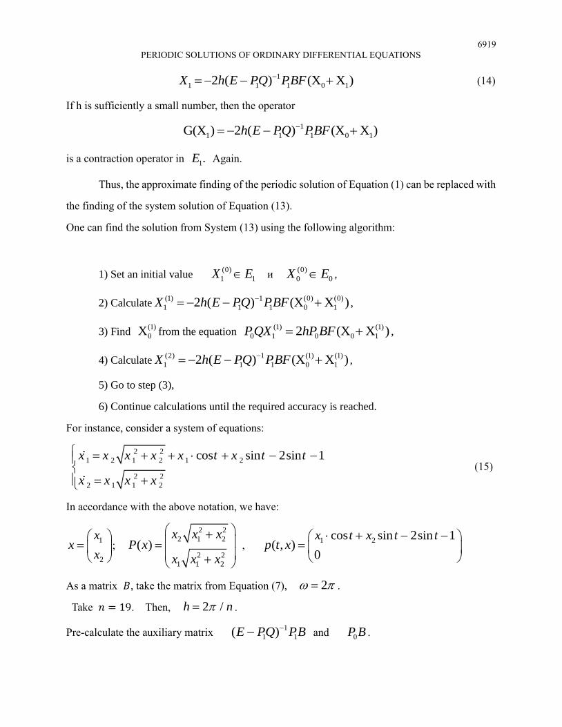
For instance, consider a system of equations:

2 2

1 2 1 2 1 2

2 2

2 1 1 2

cos sin 2sin 1x x x x x t x t t

x x x x

= + + + − −

= +

(15)

In accordance with the above notation, we have:

1

2

xx

x

=

;

2 2

2 1 2

2 2

1 1 2

( )x x x

P xx x x

+ = +

, 1 2cos sin 2sin 1

( , )0

x t x t tp t x

+ − − =

As a matrix 𝐵, take the matrix from Equation (7), 2 = .

Take 𝑛 = 19. Then, 2 /h n= .

Pre-calculate the auxiliary matrix 1

1 1( )E PQ PB−− and 0P B .

6920


After 12 iterations, the following values were obtained for 1x and 2x :

it 1x 2x it 1x 2x

0 0,934379 0,010138 3,30694 -0,92312 -0,13624

0,330694 0,879337 0,296918 3,637634 -0,82405 -0,41945

0,661388 0,729388 0,55658 3,968328 -0,63416 -0,66567

0,992082 0,503193 0,763644 4,299022 -0,3757 -0,84332

1,322776 0,225289 0,890692 4,629715 -0,07719 -0,92518

1,65347 -0,07575 0,917269 4,960409 0,229505 -0,89748

1,984164 -0,369 0,838737 5,291103 0,511823 -0,76498

2,314858 -0,62439 0,668435 5,621797 0,739255 -0,54914

2,645552 -0,81524 0,431628 5,952491 0,885971 -0,28056

2,976246 -0,91955 0,155476 3,30694 -0,92312 -0,13624

3,30694 -0,92312 -0,13624 3,637634 -0,82405 -0,41945

Table (1)

Table 1 illustrates the approximate values for 1x and 2x after 12 iterations.

The solution of the equation (1) (1)

0 1 0 0 12 (X X )PQX hP BF= + was determined with an accuracy

of up to ∆= 0.01.

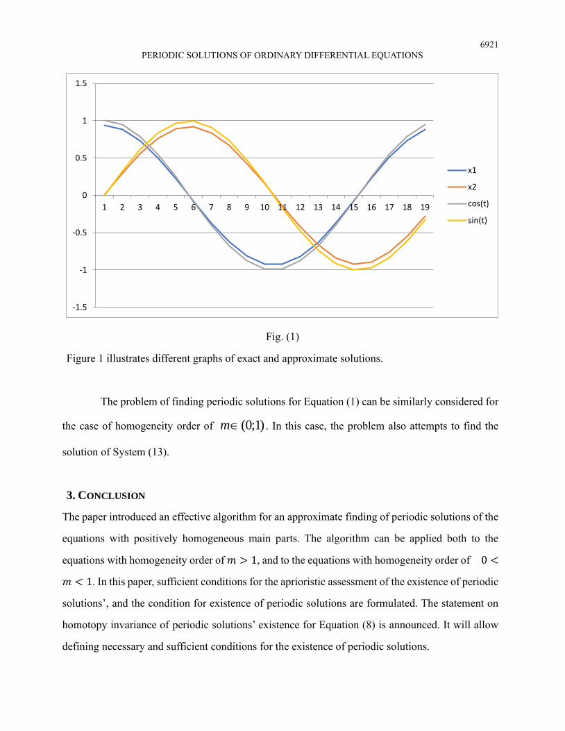
The exact solution of System (15) has the form: 1 2( ) cos ; ( ) sinx t t x t t= = .

6921


Fig. (1)

Figure 1 illustrates different graphs of exact and approximate solutions.

The problem of finding periodic solutions for Equation (1) can be similarly considered for

the case of homogeneity order of (0;1)m . In this case, the problem also attempts to find the

solution of System (13).

3. CONCLUSION

The paper introduced an effective algorithm for an approximate finding of periodic solutions of the

equations with positively homogeneous main parts. The algorithm can be applied both to the

equations with homogeneity order of 𝑚 > 1, and to the equations with homogeneity order of 0 <

𝑚 < 1. In this paper, sufficient conditions for the aprioristic assessment of the existence of periodic

solutions’, and the condition for existence of periodic solutions are formulated. The statement on

homotopy invariance of periodic solutions’ existence for Equation (8) is announced. It will allow

defining necessary and sufficient conditions for the existence of periodic solutions.

-1.5

-1

-0.5

0

0.5

1

1.5

1 2 3 4 5 6 7 8 9 10 11 12 13 14 15 16 17 18 19

x1

x2

cos(t)

sin(t)

6922


CONFLICT OF INTERESTS

The author(s) declare that there is no conflict of interests.

REFERENCES

[1] U.M. Ascher, R.M. Mattheij and R.D. Russell, Numerical Solution of Boundary Value Problems for Ordinary

Differential Equations. SIAM Publications, Philadelphia, (1995).

[2] J.P. Aubin, I. Ekeland, Applied Nonlinear Analysis. Wiley, Hoboken, (1984).

[3] N.A. Bobylev, M.A. Krasnosel'sky, Principles of affinity in nonlinear problems, J. Math. Sci. 83(4) (1997), 485-

521.

[4] N.A. Bobylev, S.V. Emel’yanov, S.K. Korovin, Geometrical methods in variational problems, Kluwer Academic

Publishers, Dordrecht (1999).

[5] S.V.E. and S.K. Korovin, Control of complex and uncertain systems: new types of feedback, Meas. Sci. Technol.

12 (2001), 653–653.

[6] M.A. Krasnosel’skii, Approximate Solution of Operator Equations, Springer, (1972).

[7] M.A. Krasnoselskii, P.P. Zabreiko, Geometrical methods of nonlinear analysis, Springer, (1984).

[8] J.H. He, Homotopy perturbation technique, Comput. Meth. Appl. Mech. Eng. 178 (1999), 257–262.

[9] J.H. He, The Homotopy perturbation method nonlinear oscillators with discontinuities, Appl. Math. Comput.

151 (2004), 287–292.

[10] N.J. Mallon, Collocation: a method for computing periodic solutions of ordinary differential equations, (DCT

rapporten; Vol. 2002.035), Technische Universiteit Eindhoven, (2002).

[11] A. Rontó, M. Rontó, Successive Approximation Techniques in Non-Linear Boundary Value Problems for

Ordinary Differential Equations, in: Handbook of Differential Equations: Ordinary Differential Equations,

Elsevier, 2008: pp. 441–592.

[12] A.M. Samoilenko, Certain questions of the theory of periodic and quasi-periodic systems, D. Sc. Dissertation,

Kiev. (1967).

http://libgen.io/ads.php?md5=ACB58B0FD59DA5DFA3FAEBE84E454756

numerical methods for finding periodic solutions of

Documents