Numerical Methods

I. Finding Roots

II. Integrating Functions

What computers can’t do

• Solve (by reasoning) general mathematical problems they can only repetitively apply arithmetic primitives to input.

• Solve problems exactly.

• Represent all numbers. Only a finite subset of the numbers between 0 and 1 can be represented.

Finding roots / solving equations

• General solution exists for equations such asax2 + bx + c = 0

The quadratic formula provides a quick answer to all quadratic equations.

However, no exact general solution (formula) exists for equations with exponents greater than 4.

Finding roots…

• Even if “exact” procedures existed, we are stuck with the problem that a computer can only represent a finite number of values… thus, we cannot “validate” our answer because it will not come out exactly

• However we can say how accurate our solution is as compared to the “exact” solution

Finding roots, continued

• Transcendental equations: involving geometric functions (sin, cos), log, exp. These equations cannot be reduced to solution of a polynomial.

• Convergence: we might imagine a “reasonable” procedure for finding solutions, but can we guarantee it terminates?

Problem-dependent decisions

• Approximation: since we cannot have exactness, we specify our tolerance to error

• Convergence: we also specify how long we are willing to wait for a solution

• Method: we choose a method easy to implement and yet powerful enough and general

• Put a human in the loop: since no general procedure can find roots of complex equations, we let a human specify a neighbourhood of a solution

Practical approach - hand calculations

• Choose method and initial guess wisely

• Good idea to start with a crude graph. If you are looking for a single root you only need one positive and one negative value

• If even a crude graph is difficult, generate a table of values and plot graph from that.

Practical approach - example

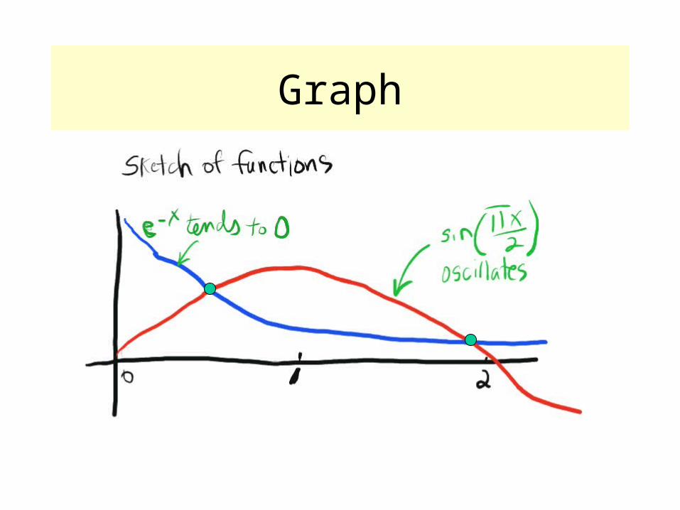
• Example e-x = sin(x/2)

• Solve for x.• Graph functions - the crossover points are

solutions• This is equivalent to finding the roots of the

difference function: f(x)= e-x - sin(x/2)

Graph

Solution, continued

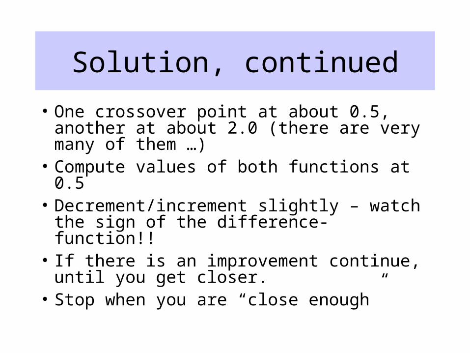
• One crossover point at about 0.5, another at about 2.0 (there are very many of them …)

• Compute values of both functions at 0.5• Decrement/increment slightly – watch the

sign of the difference-function!! • If there is an improvement continue, until

you get closer.• Stop when you are “close enough”

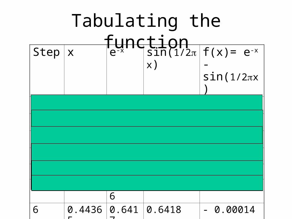
Tabulating the functionStep x e-x sin(1/2x) f(x)= e-x -

sin(1/2x)

0 0.3 0.741 0.454 0.297

1 0.4 0.670 0.588 0.082

2 0.5 0.606 0.707 - 0.101

3 0.45 0.638 0.649 - 0.012

4 0.425 0.654 0.619 0.0347

5 0.4375 0.6456 0.6344 0.01126

6 0.44365 0.6417 0.6418 - 0.00014

Bisection Method

• The Bisection Method slightly modifies “educated guess” approach of hand calculation method.

• Suppose we know a function has a root between a and b. (…and the function is continuous, … and there is only one root)

Bisection Method

• Keep in mind general approach in Computer Science: for complex problems we try to find a uniform simple systematic calculation

• How can we express the hand calculation of the preceding in this way?

• Hint: use an approach similar to the binary search…

Bisection method…

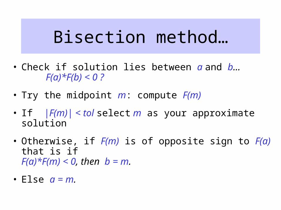
• Check if solution lies between a and b… F(a)*F(b) < 0 ?

• Try the midpoint m: compute F(m)

• If |F(m)| < tol select m as your approximate solution

• Otherwise, if F(m) is of opposite sign to F(a) that is ifF(a)*F(m) < 0, then b = m.

• Else a = m.

Bisection method…

• This method converges to any pre-specified tolerance when a single root exists on a continuous function

• Example Exercise: write a function that finds the square root of any positive number that does not require programmer to specify estimates

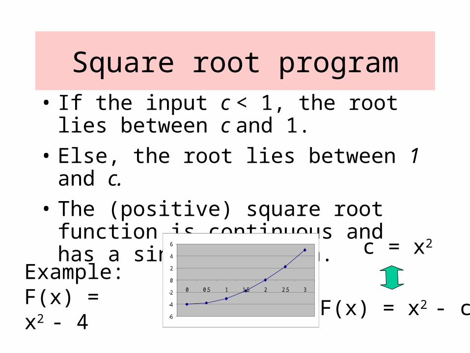
Square root program• If the input c < 1, the root lies between c

and 1.

• Else, the root lies between 1 and c.

• The (positive) square root function is continuous and has a single solution.

c = x2

F(x) = x2 - c

Example:F(x) = x2 - 4

-6

-4

-2

0

2

4

6

0 0.5 1 1.5 2 2.5 3

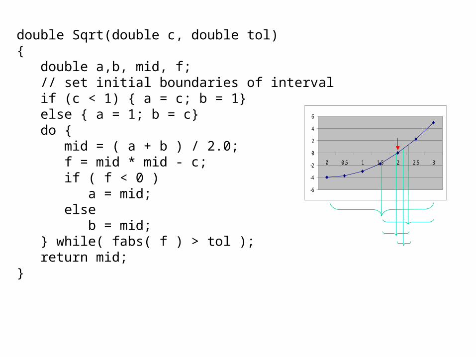
double Sqrt(double c, double tol){ double a,b, mid, f; // set initial boundaries of interval if (c < 1) { a = c; b = 1} else { a = 1; b = c} do { mid = ( a + b ) / 2.0; f = mid * mid - c; if ( f < 0 ) a = mid; else b = mid; } while( fabs( f ) > tol ); return mid;}

-6

-4

-2

0

2

4

6

0 0.5 1 1.5 2 2.5 3

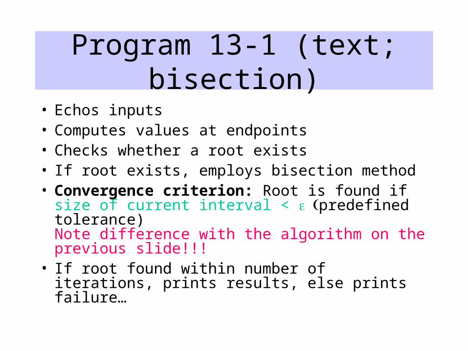
Program 13-1 (text; bisection)

• Echos inputs• Computes values at endpoints• Checks whether a root exists• If root exists, employs bisection method• Convergence criterion: Root is found if size of

current interval < predefined tolerance) Note difference with the algorithm on the previous slide!!!

• If root found within number of iterations, prints results, else prints failure…

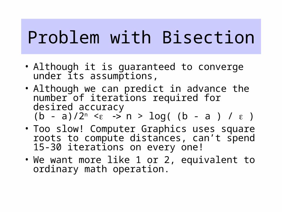
Problem with Bisection

• Although it is guaranteed to converge under its assumptions,

• Although we can predict in advance the number of iterations required for desired accuracy (b - a)/2n <n > log((b - a ) / )

• Too slow! Computer Graphics uses square roots to compute distances, can’t spend 15-30 iterations on every one!

• We want more like 1 or 2, equivalent to ordinary math operation.

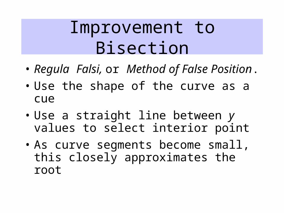
Improvement to Bisection

• Regula Falsi, or Method of False Position.

• Use the shape of the curve as a cue

• Use a straight line between y values to select interior point

• As curve segments become small, this closely approximates the root

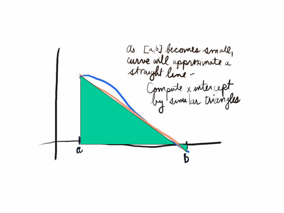
approximation

curve

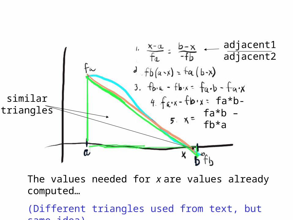
The values needed for x are values already computed…

(Different triangles used from text, but same idea)

fa*b-fb*afa*b – fb*a

similartriangles

adjacent1adjacent2

Method of false position

• Pro: as the interval becomes small, the interior point generally becomes much closer to root

• Con 1: if fa and fb become too close – overflow errors can occur

• Con 2: can’t predict number of iterations to reach a give precision

• Con 3: can be less precise than bisection – no strict precision guarantee

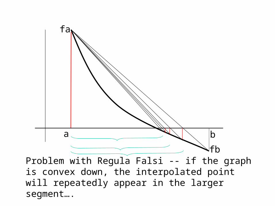
Problem with Regula Falsi -- if the graph is convex down, the interpolated point will repeatedly appear in the larger segment….

a b

fb

fa

ab

fa

fb

x

fx

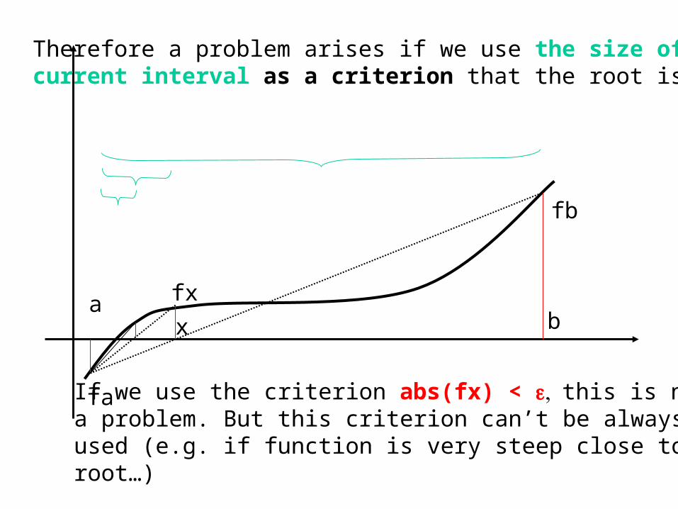
Therefore a problem arises if we use the size of the current interval as a criterion that the root is found

If we use the criterion abs(fx) < this is nota problem. But this criterion can’t be alwaysused (e.g. if function is very steep close to theroot…)

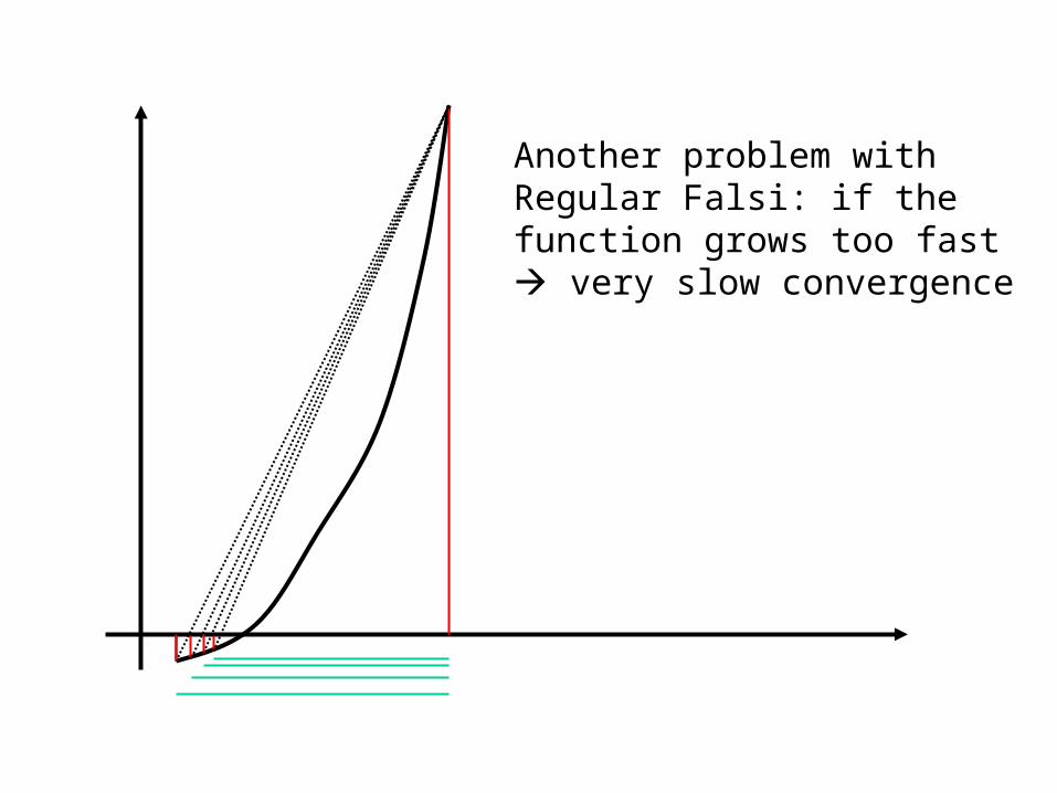
Another problem with Regular Falsi: if the function grows too fast very slow convergence

Modified Regula Falsi

• Because Regula Falsi can be fatally slow some of the time (which is too often)

• Want to clip interval from both ends

• Trick: drop the line from fa or fb to some fraction of its height, artificially change slope to cut off more of other side

• The root will flip between left and right interval

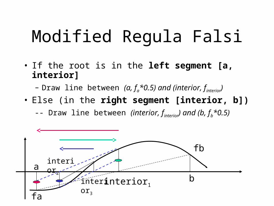
Modified Regula Falsi

• If the root is in the left segment [a, interior]– Draw line between (a, fa*0.5) and (interior, finterior)

• Else (in the right segment [interior, b])-- Draw line between (interior, finterior) and (b, fb*0.5)

abinterior1

fa

interior2

interior3

fb

Secant Method

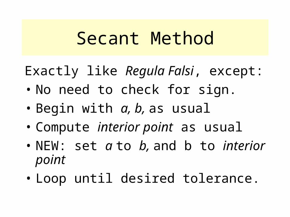
Exactly like Regula Falsi, except:

• No need to check for sign.

• Begin with a, b, as usual

• Compute interior point as usual

• NEW: set a to b, and b to interior point

• Loop until desired tolerance.

Secant method

• No animation ready yet: Intuition

• It automatically flips back and forth, solving problem with unmodified regula falsi

• Sometimes, both fa and fb are positive, but it quickly tracks secant lines to root

Secant Illustration

-20

0

20

40

60

80

100

120

1 2 3 4 5 6 7 8 9 10 11 12

Series1

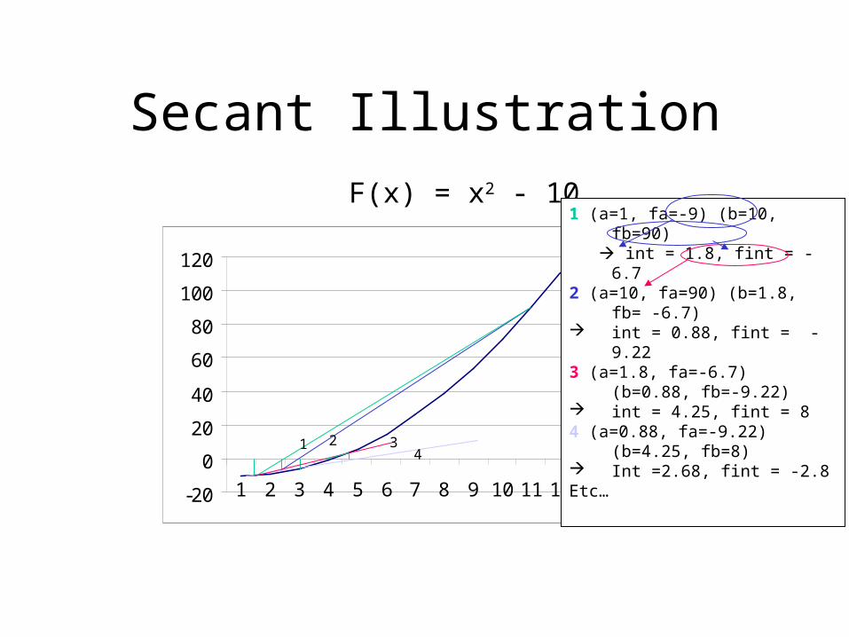
F(x) = x2 - 101 (a=1, fa=-9) (b=10, fb=90) int = 1.8, fint = -6.72 (a=10, fa=90) (b=1.8, fb= -6.7) int = 0.88, fint = -9.223 (a=1.8, fa=-6.7) (b=0.88, fb=-9.22) int = 4.25, fint = 84 (a=0.88, fa=-9.22) (b=4.25, fb=8) Int =2.68, fint = -2.8Etc…

1 24

3

Root finding algorithms

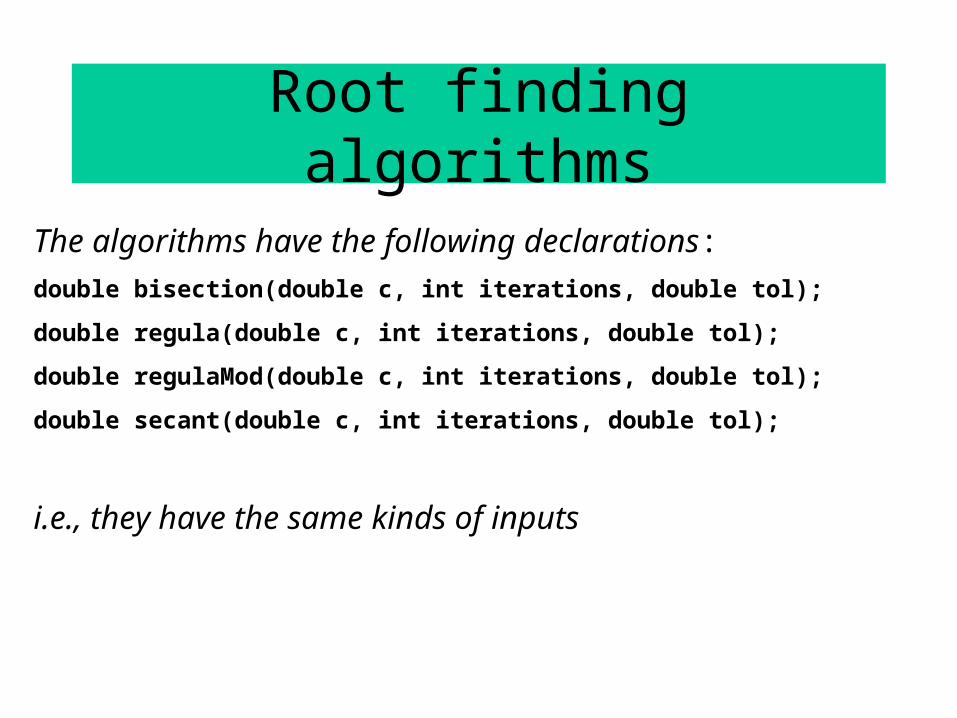
The algorithms have the following declarations:

double bisection(double c, int iterations, double tol);

double regula(double c, int iterations, double tol);

double regulaMod(double c, int iterations, double tol);

double secant(double c, int iterations, double tol);

i.e., they have the same kinds of inputs

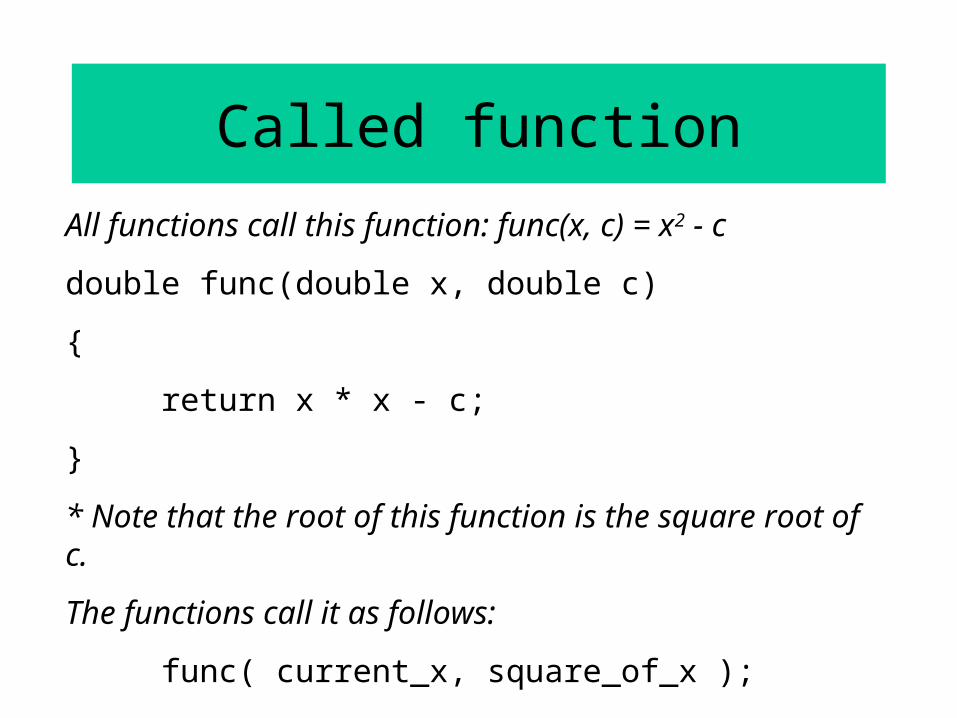
Called function

All functions call this function: func(x, c) = x2 - c

double func(double x, double c)

{

return x * x - c;

}

* Note that the root of this function is the square root of c.

The functions call it as follows:

func( current_x, square_of_x );

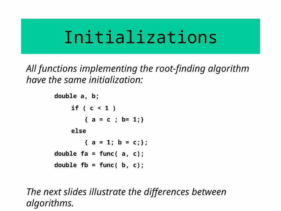
Initializations

All functions implementing the root-finding algorithm have the same initialization:

double a, b;

if ( c < 1 )

{ a = c ; b= 1;}

else

{ a = 1; b = c;};

double fa = func( a, c);

double fb = func( b, c);

The next slides illustrate the differences between algorithms.

Code

• Earlier code gave “square root” example with logic of bisection method.

• Following programs, to fit on a slide, have no debug output, and have the same initializations (as on the next slide)

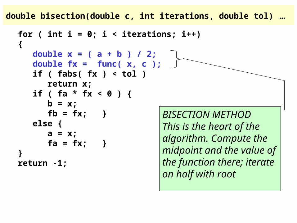
double bisection(double c, int iterations, double tol) …

for ( int i = 0; i < iterations; i++){ double x = ( a + b ) / 2; double fx = func( x, c ); if ( fabs( fx ) < tol ) return x; if ( fa * fx < 0 ) { b = x; fb = fx; } else { a = x; fa = fx; }}return -1;

BISECTION METHODThis is the heart of the algorithm. Compute the midpoint and the value of the function there; iterate on half with root

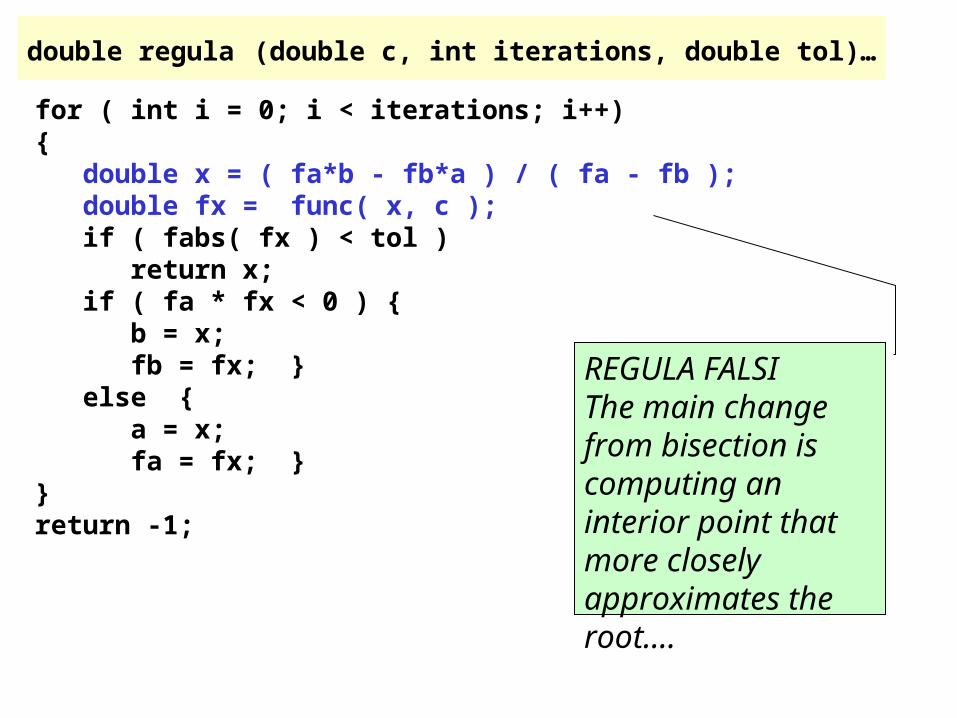
double regula (double c, int iterations, double tol)…

REGULA FALSI The main change from bisection is computing an interior point that more closely approximates the root….

for ( int i = 0; i < iterations; i++){ double x = ( fa*b - fb*a ) / ( fa - fb ); double fx = func( x, c ); if ( fabs( fx ) < tol ) return x; if ( fa * fx < 0 ) { b = x; fb = fx; } else { a = x; fa = fx; }}return -1;

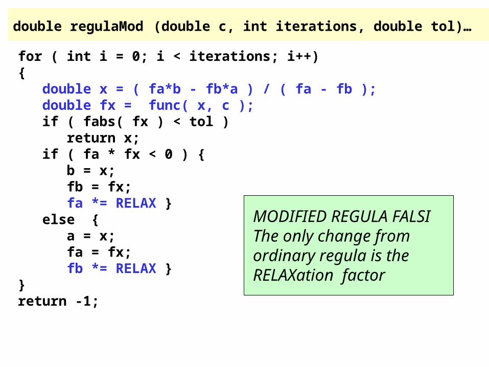
double regulaMod (double c, int iterations, double tol)…

for ( int i = 0; i < iterations; i++){ double x = ( fa*b - fb*a ) / ( fa - fb ); double fx = func( x, c ); if ( fabs( fx ) < tol ) return x; if ( fa * fx < 0 ) { b = x; fb = fx; fa *= RELAX } else { a = x; fa = fx; fb *= RELAX }}return -1;

MODIFIED REGULA FALSIThe only change from ordinary regula is theRELAXation factor

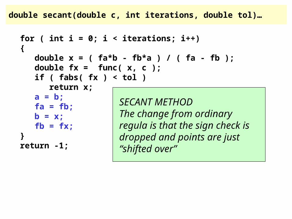
double secant(double c, int iterations, double tol)…

for ( int i = 0; i < iterations; i++){ double x = ( fa*b - fb*a ) / ( fa - fb ); double fx = func( x, c ); if ( fabs( fx ) < tol ) return x; a = b; fa = fb; b = x; fb = fx;}return -1;

SECANT METHODThe change from ordinaryregula is that the sign check is dropped and points are just “shifted over”

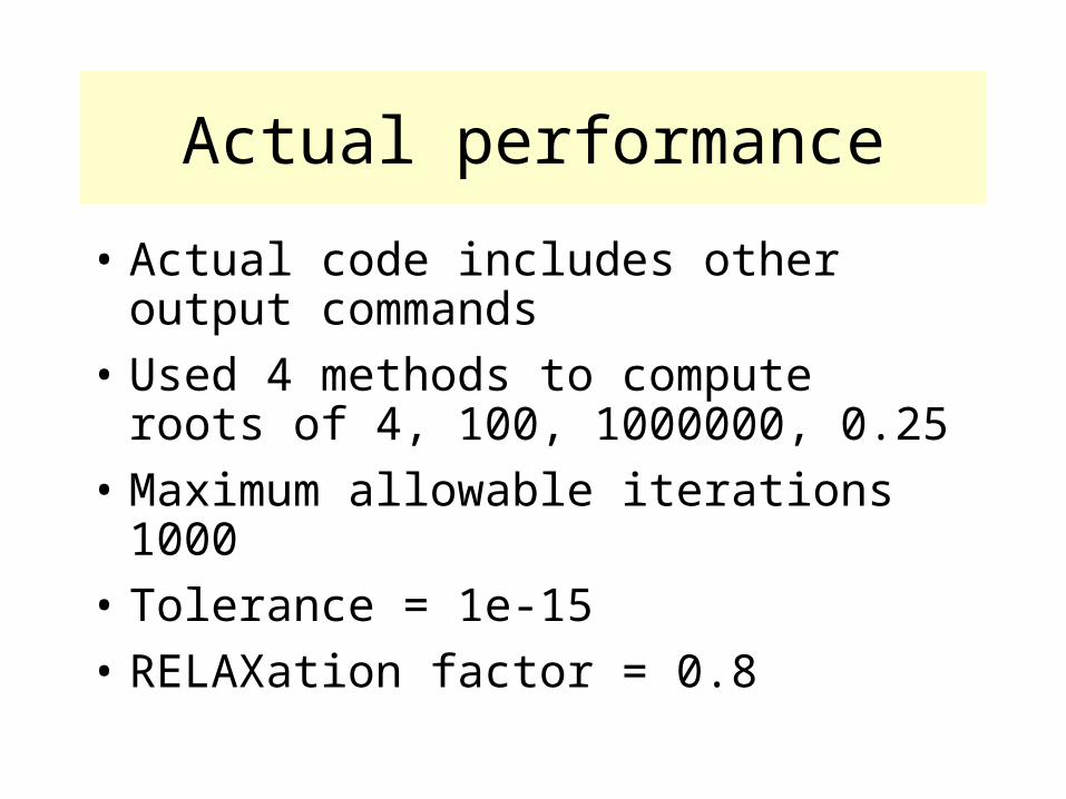
Actual performance

• Actual code includes other output commands

• Used 4 methods to compute roots of 4, 100, 1000000, 0.25

• Maximum allowable iterations 1000

• Tolerance = 1e-15

• RELAXation factor = 0.8

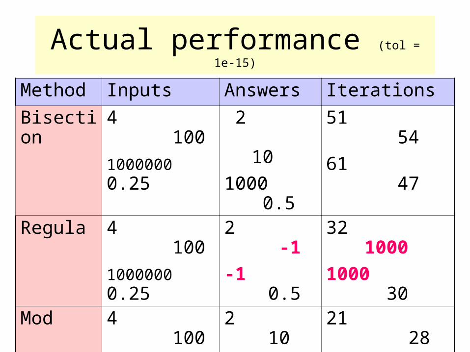
Actual performance (tol = 1e-15)

Method Inputs Answers Iterations

Bisection 4 100

1000000 0.25

2 10

1000 0.5

51 54

61 47Regula 4 100

1000000 0.25

2 -1

-1 0.5

32 1000

1000 30Mod 4 100

1000000 0.25

2 10

1000 0.5

21 28

46 19Secant 4 100

1000000 0.25

2 10

1000 0.5

7 10

20 6

Important differences from text

• Assumed all methods would be used to find square root of k between [1, c] or [c,1] by finding root of x2 – c.

• All used closeness of fx to 0 as convergence criteria. Text uses different criteria for different algorithms

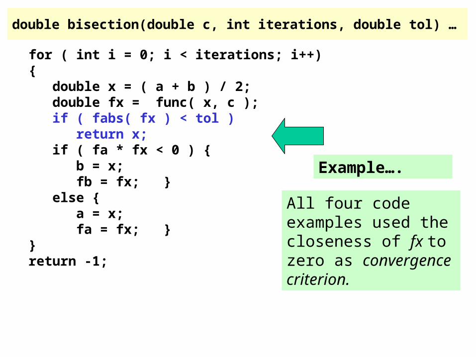
double bisection(double c, int iterations, double tol) …

for ( int i = 0; i < iterations; i++){ double x = ( a + b ) / 2; double fx = func( x, c ); if ( fabs( fx ) < tol ) return x; if ( fa * fx < 0 ) { b = x; fb = fx; } else { a = x; fa = fx; }}return -1;

Example….

All four code examples used the closeness of fx to zero as convergence criterion.

Convergence criterion…

• Closeness of fx to zero not always a good criterion, consider a very flat function may be close to zero a considerable distance before the root

Other convergence criteria

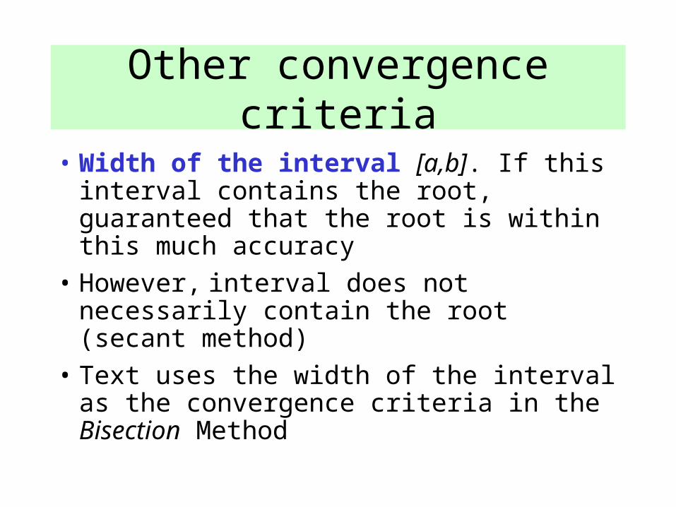
• Width of the interval [a,b]. If this interval contains the root, guaranteed that the root is within this much accuracy

• However, interval does not necessarily contain the root (secant method)

• Text uses the width of the interval as the convergence criteria in the Bisection Method

Convergence criteria…

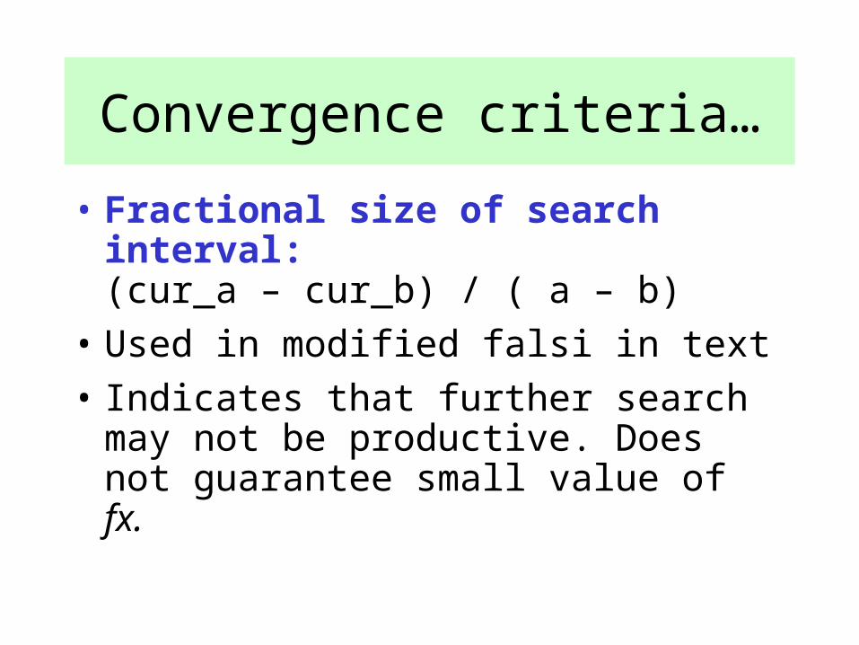
• Fractional size of search interval: (cur_a – cur_b) / ( a – b)

• Used in modified falsi in text

• Indicates that further search may not be productive. Does not guarantee small value of fx.

Numerical Integration

• In NA, take visual view of integration as area under the curve

• Many integrals that occur in science or engineering practice do not have a closed form solution – must be solved using numerical integration

Trapezoidal Rule

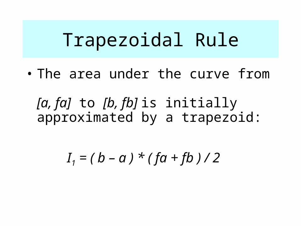
• The area under the curve from [a, fa] to [b, fb] is initially approximated by a trapezoid:

I1 = ( b – a ) * ( fa + fb ) / 2

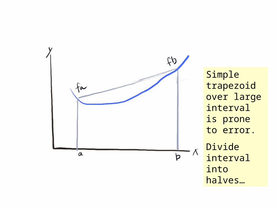
Simple trapezoid over large interval is prone to error.

Divide interval into halves…

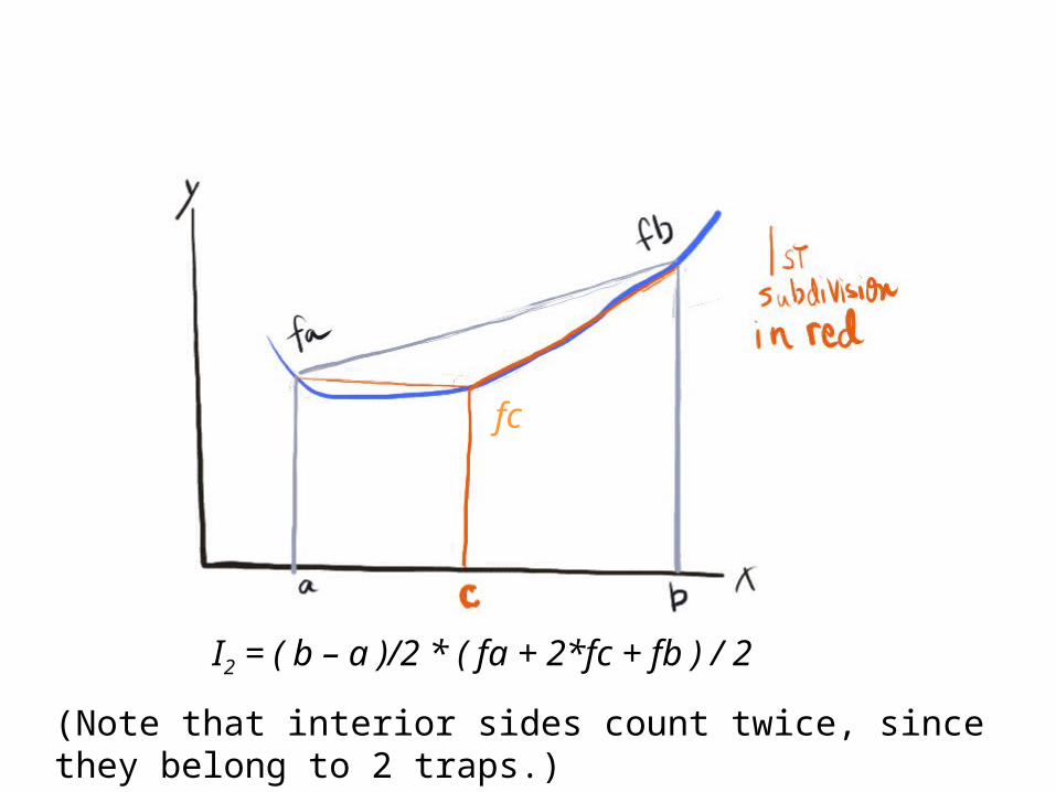
I2 = ( b – a )/2 * ( fa + 2*fc + fb ) / 2

(Note that interior sides count twice, since they belong to 2 traps.)

fc

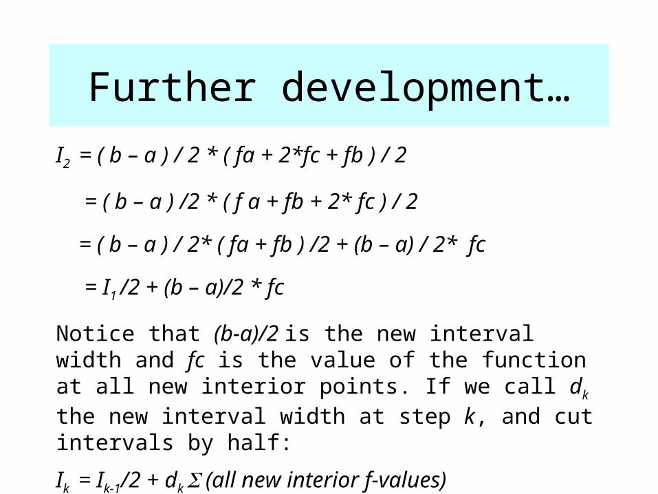
Further development…

I2 = ( b – a ) / 2 * ( fa + 2*fc + fb ) / 2

= ( b – a ) /2 * ( f a + fb + 2* fc ) / 2

= ( b – a ) / 2* ( fa + fb ) /2 + (b – a) / 2* fc

= I1 /2 + (b – a)/2 * fc

Notice that (b-a)/2 is the new interval width and fc is the value of the function at all new interior points. If we call dk the new interval width at step k, and cut intervals by half:

Ik = Ik-1/2 + dk (all new interior f-values)

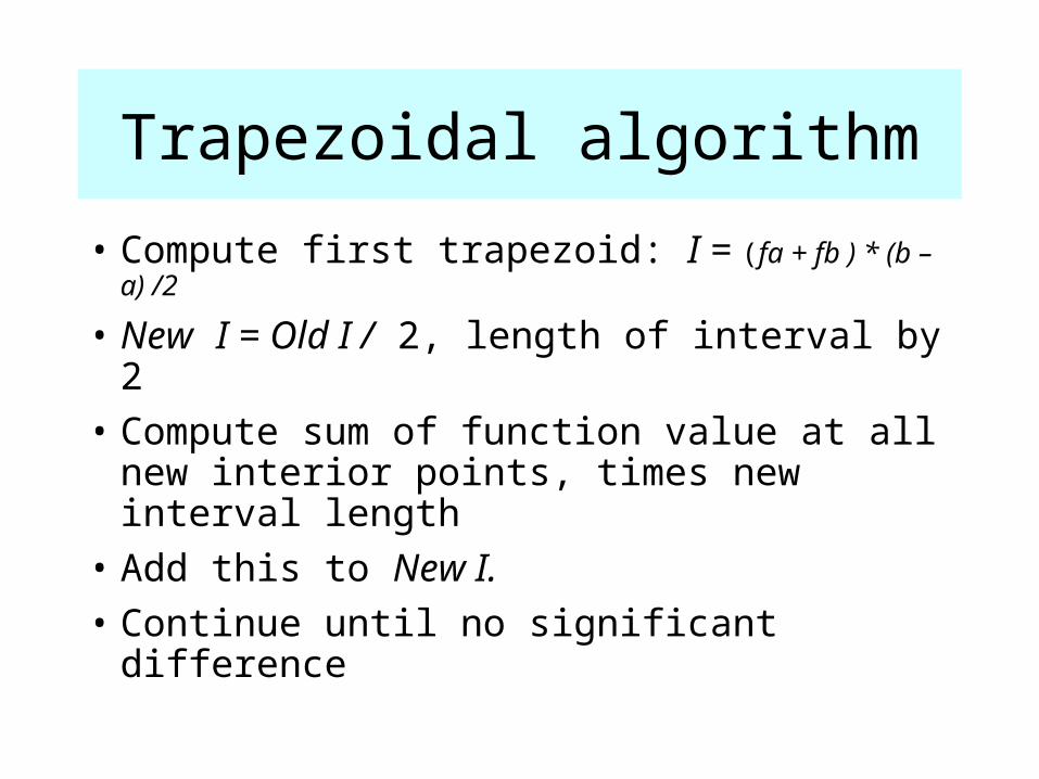
Trapezoidal algorithm

• Compute first trapezoid: I = (fa + fb ) * (b – a) /2

• New I = Old I / 2, length of interval by 2

• Compute sum of function value at all new interior points, times new interval length

• Add this to New I.

• Continue until no significant difference

Simpson’s rule

• .. Another approach

• Rather than use straight line of best fit,

• Use parabola of best fit (curves)

• Converges more quickly