Numerical Methods for ODEs

Lectures for PSU Summer Programs Xiantao Li

Outline

Introduction

ò  Numerical methods for ODEs

ò  Accuracy

ò  Stability

ò  Applications

ò  Preserving invariants

ò  Preserving symmetry

ò  Preserving geometric structures

Some Challenges

ò  Stiff ODEs

ò  Constrained dynamics

ò  Coarse-graining

ò  Multiple time scales

ò  Statistical mechanics

Ordinary Differential Equations

ò  General form

ò  Applications

ò  Mechanics

ò  Molecular models

ò  Chemical reactions

ò  Discretization of PDEs

ò  Examples from 251

ò  Mass-spring model, population model, motion in space …

ò  For most ODEs, the solutions can be obtained from analytical methods.

x

0 = f(x, t)

Numerical Solutions

ò  Exact solution

ò  Numerical solution

ò  Numerical methods

ò  Time discretization

ò  Example: uniform step size:

ò  Euler’s method:

x(t) = �(t, x(0))

x(t) = (t, x(0);�t)

⌧ = {t0, t1, · · · , tN} ⇢ [0, T ]

tj = j�t, j � 0

x(tj+1)� x(tj)

�t

= f(x(tj), tj)

A Two-Stage Runge-Kutta Method

ò  First stage:

ò  Second stage:

ò  Numerical error

ò  Higher order RK methods are available (try rk45 in Matlab)

k1 = f(x(tj), tj), x(tj+1)⇤ = x(tj) +�tk1

k2 = f(x(tj+1)⇤, tj+1), x(tj+1) = x(tj) +

�t

2

⇥k1 + k2

⇤

k�(t)� (t)k �t2eLt.

Inheritance of Asymptotic Stability

ò  For a linear system, is stable if all eigenvalues of A are negative.

ò  For a nonlinear system, , an equilibrium is stable if the eigenvalues of are negative.

ò  A numerical method is stable if the stability of the linear system is inherited.

ò  Typically, the step size has to be sufficiently small (inverse proportional to the eigenvalues) in order for the method to be stable.

ò  The problem becomes stiff when some eigenvalues are large.

x

0 = Ax, x = 0

x

0 = f(x) x0

rf(x0)

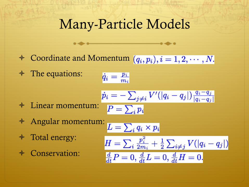
Many-Particle Models

ò  Coordinate and Momentum

ò  The equations:

ò  Linear momentum:

ò  Angular momentum:

ò  Total energy:

ò  Conservation:

First Integrals (Invariants)

ò  In general, for

ò  is a first integral if

ò  Most numerical methods preserve linear invariant

ò  Only some methods preserve quadratic invariants

ò  In general, it is not possible to exactly preserve invariants of higher order.

Symmetry

ò  If the function is symmetric wrt

ò  The solutions of the ODEs will be called ρ- reversible

ò 

ò  For example,

ò  A numerical method is ρ- reversible if the solution satisfies the same properties.

ò  Explicit RK methods are not symmetric.

Symplectic Structure

ò  A linear mapping A is symplectic if

ò  A nonlinear mapping g is symplectic if

Hamiltonian systems

ò  Hamilton’s principle

ò  Examples: mass spring model, many-body problems, pendulum model, Lotka-Volterra model etc.

ò  The mapping is symplectic

ò  A numerical method is symplectic if it defines a symplectic mapping

Symmetric and symplectic methods

ò  Symmetric methods

ò  Order of accuracy is always even

ò  Very convenient for an extrapolation procedure

ò  Symplectic methods

ò  Very good energy conservation properties

ò  Promising accuracy over long time integration

ò  Provide good statistics.

Dimension Reduction: I

ò  A Hamiltonian system

ò  Imposing constraints

ò  Effectively, there are only n free variables

ò  Example: flexible pendulum

y0 = JrH(y)

c(y) = 0, c : RN ! RN�n

CSE/MATH Homework 3

Due Oct 14, 2008

1. 6.4, pp 306.

2. 6.9, pp 306.

3. Consider a pendulum system consisting of a point mass m and a massless spring with springconstant 1

!2 . x = (x1, x2) and (mv1,mv2) are used as the coordinate and momenta for the mass

respectively. The total energy of the system is given by,

H = K + U =1

2(mv2

1 + mv22) + mgx2 +

1

2!2

!

"

x21+ x2

2! l)2,

where l is the natural length of the spring and g denotes the gravity. The equation of motion forthe mass is given by,

mx!! = !"U.

Choose the parameters m = 1, l = 1, g = 1, and ! = 10"5. Integrate the system using the three-stage Runge-Kutta-Gauss method with stepsize !t = 0.01 until T = 20. Initially the mass is heldat x0. Choose x0 = (l, 0) and x0 = (l + !, 0). For the numerical output, plot the position (bothcomponents), velocity (both components), and total energy.

4. The system,#

$

%

x!

1 = !K1x1x2 + K2x3,

x!

2 = !K1x1x2 + K2x3 ! K3x2x3,

x!

3 = K1x1x2 ! K2x3 ! K3x2x3,

describes a chemical process. x1 and x2 represent the concentration of the species A and B, and x3

represents the concentration of an intermediate species X. Solve these di"erential equations usingthe two-stage and three-stage Runge-Kutta-Radau method. For the computer simulation, pick theparameters K1 = K2 = 0.1, K3 = 100, the step size !t = 0.05, T = 100, initial condition (1, 1, 0).Compare the results to an explicit method.

1

Dimension Reduction: II

ò  A large system

ò  Some quantities of interest

ò  Remaining degrees of freedom:

ò  Effective equation:

ò  S(t): memory function

ò  R(t): random noise

x

0 = �Ax, x 2 RN, A 2 RN⇥N

, N � 1.

y = Bx, y 2 Rn, B 2 Rn⇥N

z = Cx, z 2 RN�n, B 2 R(N�n)⇥N

My0 = �Ky +

Z t

0S(t� s)y(s)ds+R(t)

Summer Project I

ò  Minimum energy path (MEP)

ò  The most efficient path from one stable state to another

ò  The most probable path

ò  Represents rare but important events

ò  ODEs with boundary conditions

Summer Project II

ò  ODEs with multiple time scales

ò  An example,

ò  A multiscale method targeting the slow variables only

ò  Large time step size

⇢x

0 = f(x, y)y

0 = � 1" (y � '(x))