Numerical Methods in Computational Fluid Dynamics (CFD)

Zhaoyuan Wang, Maysam Mousaviraad, Tao Xing and Fred Stern

IIHR—Hydroscience & Engineering

C. Maxwell Stanley Hydraulics Laboratory

The University of Iowa

ME:5160 Intermediate Mechanics of Fluids

http://css.engineering.uiowa.edu/~me_160/

Oct. 11, 2019

2

Outline

1. Introduction to Numerical Methods2. Components of Numerical Methods

2.1. Properties of Numerical Methods2.2. Discretization Methods2.3. Application of Numerical methods in PDE 2.4. Numerical Grid and Coordinates2.5. Solution of Linear Equation System2.6. Convergence Criteria

3. Methods for Unsteady Problems4. Solution of Navier-Stokes Equations5. Example

3

Introduction to numerical methods• Approaches to Fluid Dynamical Problems:

1. Simplifications of the governing equations AFD

2. Experiments on scale models EFD

3. Discretize governing equations and solve by computers CFD

• CFD is the simulation of fluids engineering system using modeling and numerical methods

• Possibilities and Limitations of Numerical Methods:

1. Coding level: quality assurance, programming

defects, inappropriate algorithm, etc.

2. Simulation level: iterative error, truncation error, grid

error, etc.

4

Components of numerical methods (Properties)

• Consistence1. The discretization should become exact as the grid spacing

tends to zero2. Truncation error: Difference between the discretized equation

and the exact one

• Stability: does not magnify the errors that appear in the course of numerical solution process.1. Iterative methods: not diverge

2. Temporal problems: bounded solutions3. Von Neumann’s method4. Difficulty due to boundary conditions and non-linearities

present.

• Convergence: solution of the discretized equations tends to the exact solution of the differential equation as the grid spacing tends to zero.

5

• Conservation1. The numerical scheme should on both local and global basis respect the conservation laws.

2. Automatically satisfied for control volume method, either individual control volume or the whole domain.

3. Errors due to non-conservation are in most cases appreciable only on relatively coarse grids, but hard to estimate quantitatively

• Boundedness:1. Numerical solutions should lie within proper bounds (e.g. non-negative density and TKE for turbulence; concentration between 0% and 100%, VOF between 0 and 1, etc.)2. Difficult to guarantee, especially for higher order schemes.

• Realizability: models of phenomena which are too complex to treat directly (turbulence, combustion, or multiphase flow) should be designed to guarantee physically realistic solutions.

• Accuracy: 1. Modeling error 2. Discretization errors 3. Iterative errors

Components of numerical methods (Properties, Cont’d)

6

Components of numerical methods (Discretization Methods)

• Finite Difference Method (focused in this lecture)1. Introduced by Euler in the 18th century.

2. Governing equations in differential form domain with gridreplacing the partial derivatives by approximations in terms of node values of the functions one algebraic equation per grid node linear algebraic equation system.

3. Applied to structured grids

• Finite Volume Method (not focused in this lecture)1. Governing equations in integral form solution domain is subdivided into a finite number of contiguous control volumesconservation equation applied to each CV.2. Computational node locates at the centroid of each CV.3. Applied to any type of grids, especially complex geometries4. Compared to FD, FV with methods higher than 2nd order will be difficult, especially for 3D. Good mass conservation.

• Finite Element Method (not covered in this lecture):1. Similar to FV2. Equations are multiplied by a weight function before integrated over the entire domain. Often used for Solid Mechanics.

7

Discretization methods (Finite Difference, introduction)

• First step in obtaining a numerical solution is to discretize the geometric domain to define a

numerical grid

• Each node has one unknown and need one algebraic equation, which is a relation between the variable value at that node and those at some of the neighboring nodes.

• The approach is to replace each term of the PDE at the particular node by a finite-difference approximation.

• Numbers of equations and unknowns must be equal

8

Discretization methods (Finite Difference, approximation of the first derivative)

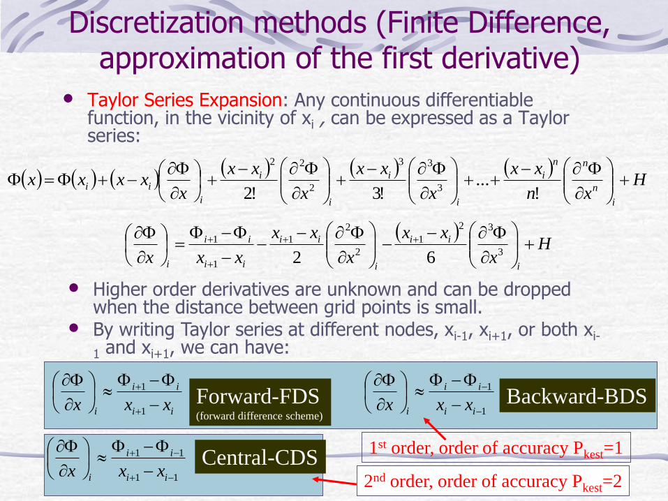
• Taylor Series Expansion: Any continuous differentiable function, in the vicinity of xi , can be expressed as a Taylor series:

Hxn

xx

x

xx

x

xx

xxxxx

i

n

nn

i

i

i

i

i

i

ii

!...

!3!2 3

33

2

22

H

x

xx

x

xx

xxxi

ii

i

ii

ii

ii

i

3

32

1

2

2

1

1

1

62

• Higher order derivatives are unknown and can be dropped when the distance between grid points is small.

• By writing Taylor series at different nodes, xi-1, xi+1, or both xi-

1 and xi+1, we can have:

ii

ii

i xxx

1

1

1

1

ii

ii

i xxx

11

11

ii

ii

i xxx

Forward-FDS(forward difference scheme)

Backward-BDS

Central-CDS1st order, order of accuracy Pkest=1

2nd order, order of accuracy Pkest=2

9

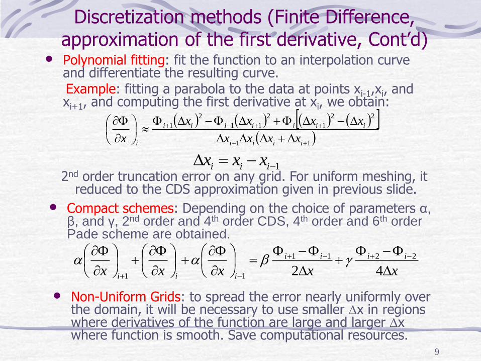
Discretization methods (Finite Difference, approximation of the first derivative, Cont’d)

• Polynomial fitting: fit the function to an interpolation curve and differentiate the resulting curve.Example: fitting a parabola to the data at points xi-1,xi, and xi+1, and computing the first derivative at xi, we obtain:

• Compact schemes: Depending on the choice of parameters α, β, and γ, 2nd order and 4th order CDS, 4th order and 6th order Pade scheme are obtained.

11

22

1

2

11

2

1

iiii

iiiiiii

i xxxx

xxxx

x

1 iii xxx2nd order truncation error on any grid. For uniform meshing, it

reduced to the CDS approximation given in previous slide.

xxxxx

iiii

iii

42

2211

11

• Non-Uniform Grids: to spread the error nearly uniformly over the domain, it will be necessary to use smaller x in regions where derivatives of the function are large and larger x where function is smooth. Save computational resources.

10

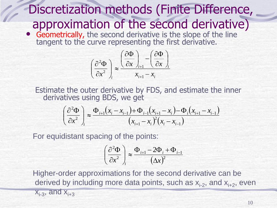
Discretization methods (Finite Difference, approximation of the second derivative)

• Geometrically, the second derivative is the slope of the line tangent to the curve representing the first derivative.

ii

ii

ixx

xx

x

1

1

2

2

Estimate the outer derivative by FDS, and estimate the inner derivatives using BDS, we get

For equidistant spacing of the points:

1

2

1

111111

2

2

iiii

iiiiiiiii

ixxxx

xxxxxx

x

211

2

2 2

xx

iii

i

Higher-order approximations for the second derivative can be

derived by including more data points, such as xi-2, and xi+2, even

xi-3, and xi+3

11

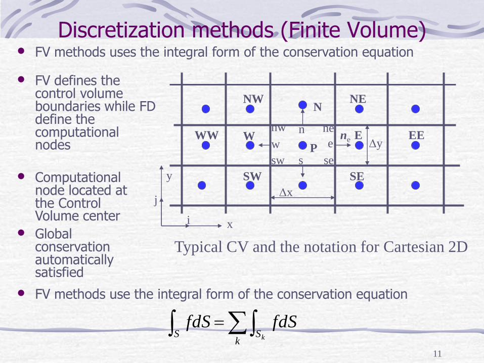
Discretization methods (Finite Volume)

WP

WW E EE

N

Typical CV and the notation for Cartesian 2D

n nenw

sesw

ew

s

x

yne

NW NE

SW SE

x

y

i

j

• FV defines the control volume boundaries while FD define the computational nodes

• Computational node located at the Control Volume center

• Global conservation automatically satisfied

• FV methods uses the integral form of the conservation equation

• FV methods use the integral form of the conservation equation

k

SS k

fdSfdS

12

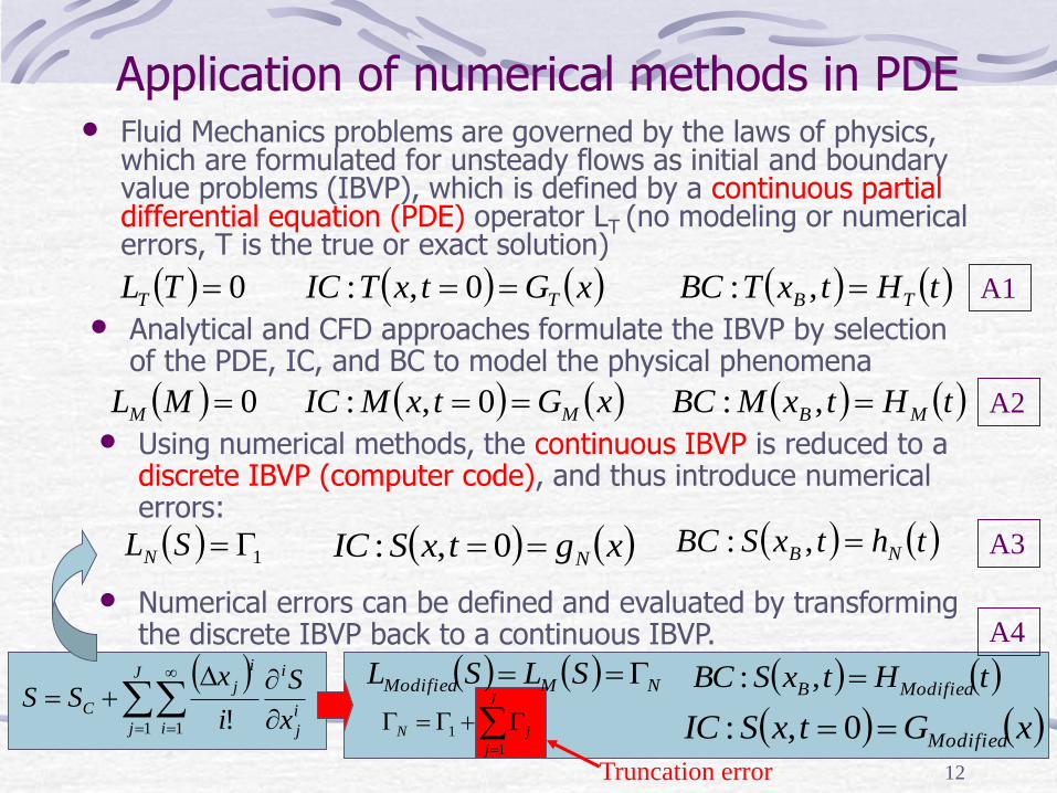
Application of numerical methods in PDE • Fluid Mechanics problems are governed by the laws of physics,

which are formulated for unsteady flows as initial and boundary value problems (IBVP), which is defined by a continuous partial differential equation (PDE) operator LT (no modeling or numerical errors, T is the true or exact solution)

• Analytical and CFD approaches formulate the IBVP by selection of the PDE, IC, and BC to model the physical phenomena

• Using numerical methods, the continuous IBVP is reduced to a discrete IBVP (computer code), and thus introduce numerical errors:

• Numerical errors can be defined and evaluated by transforming the discrete IBVP back to a continuous IBVP.

0TLT tHtxTBC TB ,: xGtxTIC T 0,:

0MLM xGtxMIC M 0,: tHtxMBC MB ,:

1SLN xgtxSIC N 0,: thtxSBC NB ,:

i

j

iJ

j i

i

j

Cx

S

i

xSS

1 1 !

NMModified SLSL

xGtxSIC Modified 0,:

tHtxSBC ModifiedB ,:

J

j

jN

1

1

Truncation error

A1

A2

A3

A4

13

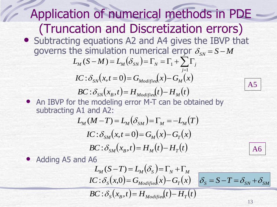
Application of numerical methods in PDE (Truncation and Discretization errors)

• Subtracting equations A2 and A4 gives the IBVP that governs the simulation numerical error

J

j

jNSNMM LMSL1

1)(

• An IBVP for the modeling error M-T can be obtained by subtracting A1 and A2:

xGxGtxIC MModifiedSN 0,:

tHtHtxBC MModifiedBSN ,:

MSSN

TLLTML MMSMMM )(

xGxGtxIC TMSM 0,:

tHtHtxBC TMBSM ,:

A5

A6

• Adding A5 and A6 MNSMM LTSL )(

xGxGxIC TModifiedS 0,:

tHtHtxBC TModifiedBS ,:

SMSNS TS

14

Numerical grids and coordinates

• The discrete locations at which the variables are to be calculated are defined by the numerical grid

• Numerical grid is a discrete representation of the geometric domain on which the problem is to be solved. It divides the solution domain into a finite number of sub-domains

• Type of numerical grids: 1. structured (regular grid), 2. Block-structured grids, and 3. Unstructured grids

• Detailed explanations of numerical grids will be presented in the last lecture of this CFD lecture series.

• Different coordinates have been covered in “Introduction to CFD”

15

Components of numerical methods(Solution of linear equation systems, introduction)

• The result of the discretization using either FD or FV, is a system of algebraic equations, which are linear or non-linear

• For non-linear case, the system must be solved using iterative methods, i.e. initial guessiterate converged results obtained.

• The matrices derived from partial differential equations are always sparse with the non-zero elements of the matrices lie on a small number of well-defined diagonals

QA

16

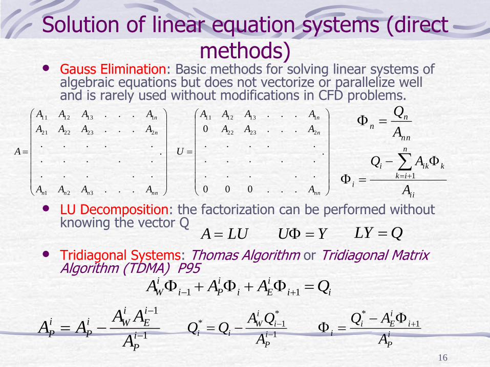
Solution of linear equation systems (direct methods)

• Gauss Elimination: Basic methods for solving linear systems of algebraic equations but does not vectorize or parallelize well and is rarely used without modifications in CFD problems.

• LU Decomposition: the factorization can be performed without knowing the vector Q

• Tridiagonal Systems: Thomas Algorithm or Tridiagonal Matrix Algorithm (TDMA) P95

ii

i

Ei

i

Pi

i

W QAAA 11

1

1

i

P

i

E

i

Wi

P

i

PA

AAAA

1

*

1*

i

P

i

i

Wii

A

QAQQ

i

P

i

i

Eii

A

AQ 1

*

.

...

.....

.....

.....

...

...

321

2232221

1131211

nnnnn

n

n

AAAA

AAAA

AAAA

A

.

...000

.....

.....

.....

...0

...

22322

1131211

nn

n

n

A

AAA

AAAA

U

nn

nn

A

Q

ii

n

ik

kiki

iA

AQ

1

LUA YU QLY

17

Solution of linear equation systems (iterative methods)

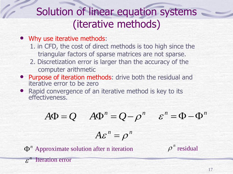
• Why use iterative methods: 1. in CFD, the cost of direct methods is too high since the

triangular factors of sparse matrices are not sparse. 2. Discretization error is larger than the accuracy of the

computer arithmetic• Purpose of iteration methods: drive both the residual and

iterative error to be zero• Rapid convergence of an iterative method is key to its

effectiveness.

QA nn QA

nn

nnA

Approximate solution after n iterationn residualn

n Iteration error

18

Solution of linear equation systems (iterative methods, cont’d)

• Typical iterative methods: 1. Jacobi method2. Gauss-Seidel method3. Successive Over-Relaxation (SOR), or LSOR4. Alternative Direction Implicit (ADI) method5. Conjugate Gradient Methods6. Biconjugate Gradients and CGSTAB7. Multigrid Methods

19

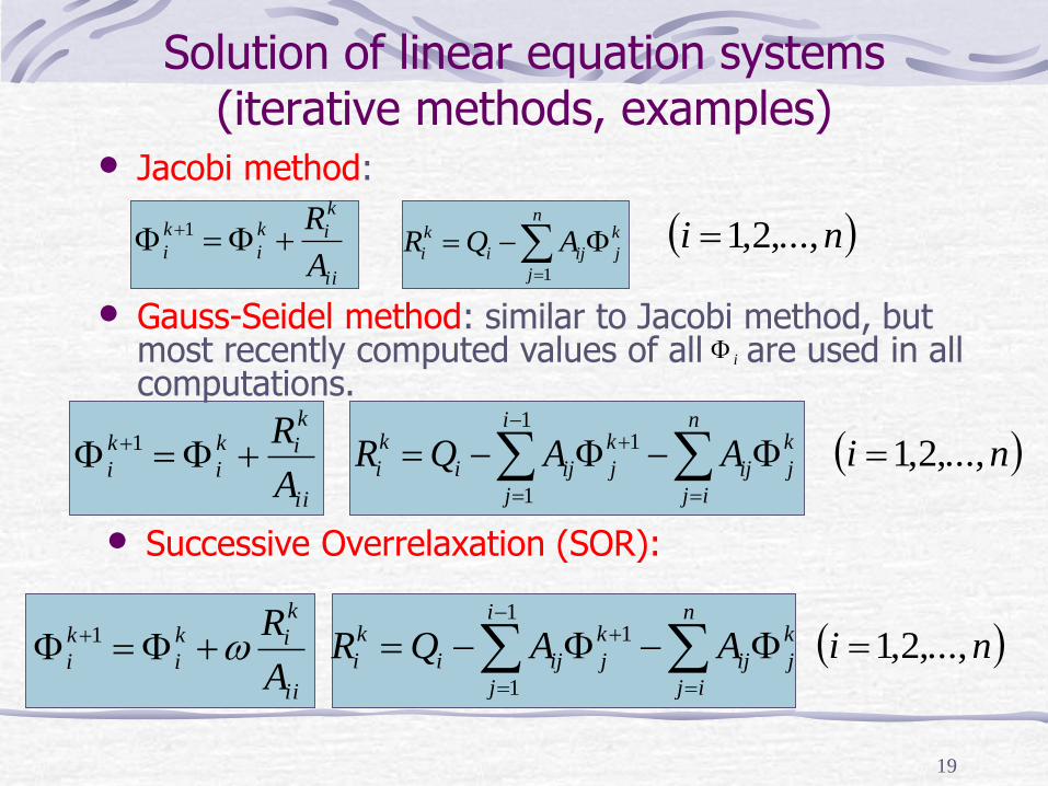
Solution of linear equation systems (iterative methods, examples)

• Jacobi method:

ii

k

ik

i

k

iA

R 1

1

nk k

i i ij j

j

R Q A

• Gauss-Seidel method: similar to Jacobi method, but most recently computed values of all are used in all computations.

ni ,...,2,1

i

ii

k

ik

i

k

iA

R 1

11

1

i nk k k

i i ij j ij j

j j i

R Q A A

ni ,...,2,1

• Successive Overrelaxation (SOR):

ii

k

ik

i

k

iA

R 1

11

1

i nk k k

i i ij j ij j

j j i

R Q A A

ni ,...,2,1

20

Solution of linear equation systems (coupled equations and their solutions)

• Definition: Most problems in fluid dynamics require solution of coupled systems of equations, i.e. dominant variable of each equation occurs in some of the other equations

• Solution approaches:1. Simultaneous solution: all variables are solved for

simultaneously2. Sequential Solution: Each equation is solved for

its dominant variable, treating the other variablesas known, and iterating until the solution isobtained.

• For sequential solution, inner iterations and outer iterations are necessary

21

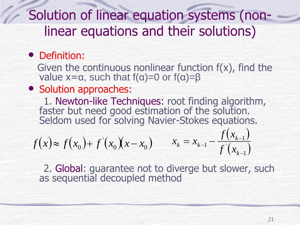
Solution of linear equation systems (non-linear equations and their solutions)

• Definition: Given the continuous nonlinear function f(x), find the value x=α, such that f(α)=0 or f(α)=β

• Solution approaches:1. Newton-like Techniques: root finding algorithm,

faster but need good estimation of the solution. Seldom used for solving Navier-Stokes equations.

2. Global: guarantee not to diverge but slower, such as sequential decoupled method

00

'

0 xxxfxfxf 1

'

11

k

kkk

xf

xfxx

22

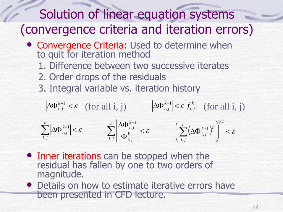
Solution of linear equation systems (convergence criteria and iteration errors)• Convergence Criteria: Used to determine when

to quit for iteration method1. Difference between two successive iterates2. Order drops of the residuals3. Integral variable vs. iteration history

• Inner iterations can be stopped when the residual has fallen by one to two orders of magnitude.

• Details on how to estimate iterative errors have been presented in CFD lecture.

1

,

k

ji

k

ji

k

ji f ,

1

,

n

ji

k

ji

,

1

,

n

jik

ji

k

ji

, ,

1

,

21

,

21

,

n

ji

k

ji

(for all i, j) (for all i, j)

23

Methods for unsteady problems (introduction)

• Unsteady flows have a fourth coordinate direction–time, which must be discretized.

• Differences with spatial discretization: a force at any space location may influence the flow anywhere else, forcing at a given instant will affect the flow only in the future (parabolic like).

• These methods are very similar to ones applied to initial value problems for ordinary differential equations.

•The basic problem is to find the solution a short time t after the initial point. The solution at t1=t0+ t, can be used as a new initial condition and the solution can be advanced to t2=t1+ t , t3=t2+ t, ….etc.

24

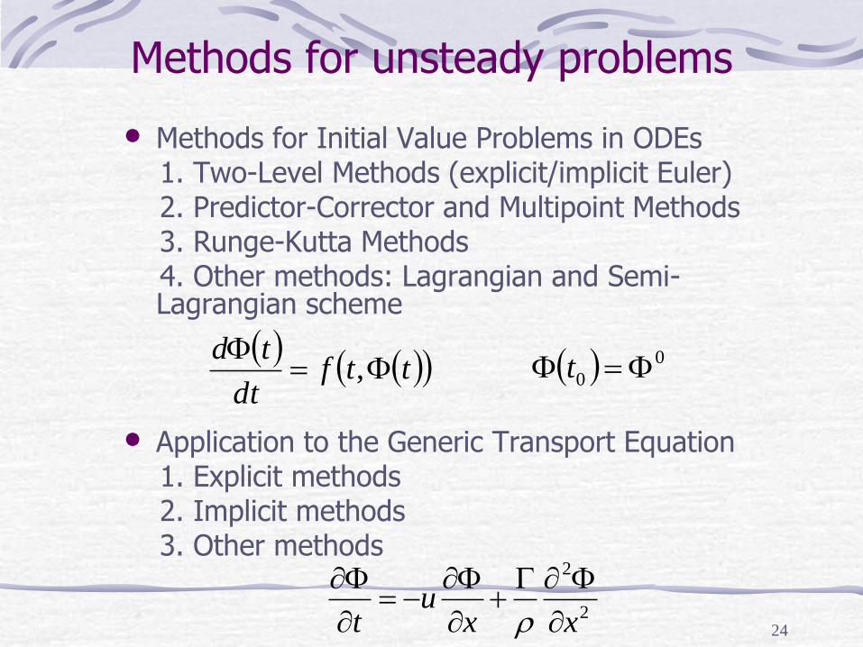
Methods for unsteady problems

• Methods for Initial Value Problems in ODEs1. Two-Level Methods (explicit/implicit Euler)2. Predictor-Corrector and Multipoint Methods3. Runge-Kutta Methods4. Other methods: Lagrangian and Semi-Lagrangian scheme

• Application to the Generic Transport Equation1. Explicit methods2. Implicit methods3. Other methods

2

2

xxu

t

ttf

dt

td

, 0

0 t

25

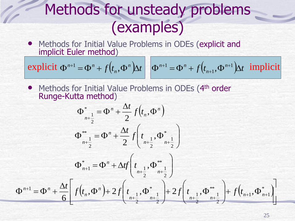
Methods for unsteady problems (examples)

• Methods for Initial Value Problems in ODEs (4th orderRunge-Kutta method)

n

n

n

ntf

t

,

2

*

2

1

*

2

1

2

1

**

2

1 ,2 nn

n

ntf

t

**

2

1

2

1

*

1 ,nn

n

n ttf

*

11

**

2

1

2

1

*

2

1

2

1

1 ,,2,2,6

nnnnnn

n

n

nn tftftftft

• Methods for Initial Value Problems in ODEs (explicit and implicit Euler method)

ttf n

n

nn ,1explicit ttf n

n

nn

1

1

1 , implicit

26

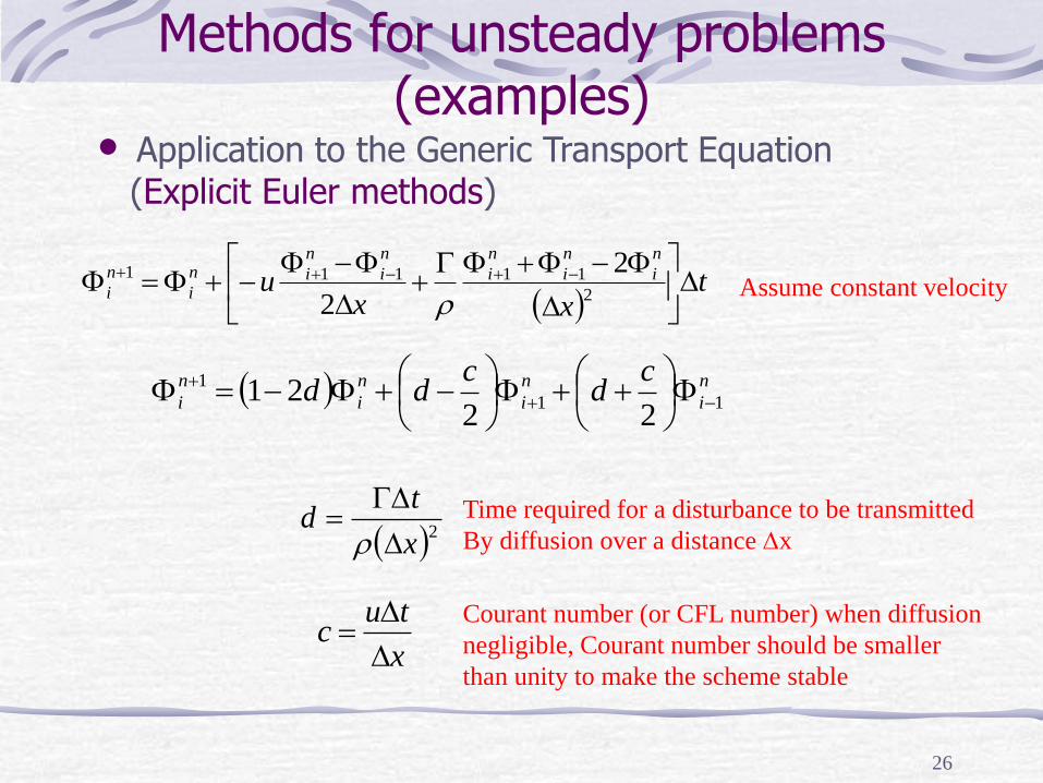
Methods for unsteady problems (examples)

• Application to the Generic Transport Equation(Explicit Euler methods)

t

xxu

n

i

n

i

n

i

n

i

n

in

i

n

i

2

11111 2

2 Assume constant velocity

n

i

n

i

n

i

n

i

cd

cdd 11

1

2221

2x

td

x

tuc

Courant number (or CFL number) when diffusion

negligible, Courant number should be smaller

than unity to make the scheme stable

Time required for a disturbance to be transmitted

By diffusion over a distance x

27

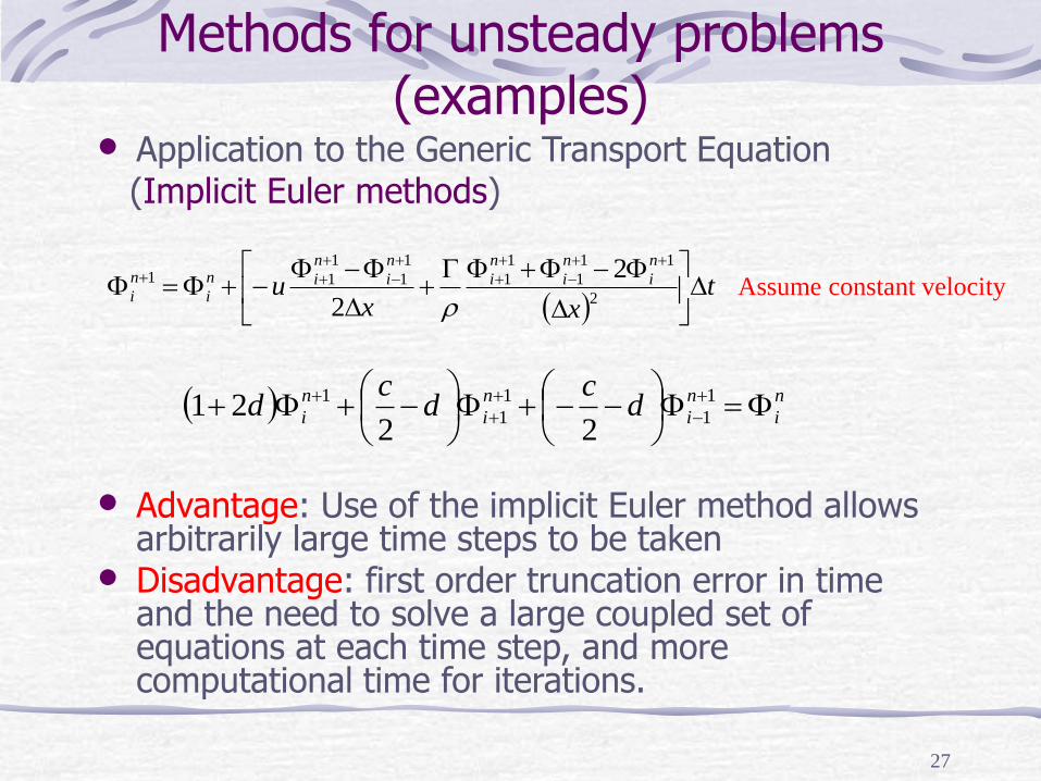
Methods for unsteady problems (examples)

• Application to the Generic Transport Equation(Implicit Euler methods)

t

xxu

n

i

n

i

n

i

n

i

n

in

i

n

i

2

11

1

1

1

1

1

1

11 2

2 Assume constant velocity

n

i

n

i

n

i

n

i dc

dc

d

1

1

1

1

1

2221

• Advantage: Use of the implicit Euler method allows arbitrarily large time steps to be taken

• Disadvantage: first order truncation error in time and the need to solve a large coupled set of equations at each time step, and more computational time for iterations.

28

Solution of Navier-Stokes equations

• Special features of Navier-Stokes Equations

• Choice of Variable Arrangement on the Grid

• Pressure Poisson equation

• Solution methods for N-S equations

29

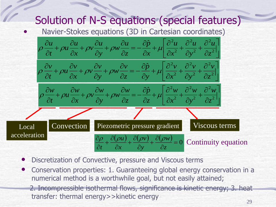
Solution of N-S equations (special features)• Navier-Stokes equations (3D in Cartesian coordinates)

2

2

2

2

2

2ˆ

z

u

y

u

x

u

x

p

z

uw

y

uv

x

uu

t

u

2

2

2

2

2

2ˆ

z

v

y

v

x

v

y

p

z

vw

y

vv

x

vu

t

v

0

z

w

y

v

x

u

t

Convection Piezometric pressure gradient Viscous termsLocal

accelerationContinuity equation

2

2

2

2

2

2ˆ

z

w

y

w

x

w

z

p

z

ww

y

wv

x

wu

t

w

• Discretization of Convective, pressure and Viscous terms

• Conservation properties: 1. Guaranteeing global energy conservation in a numerical method is a worthwhile goal, but not easily attained;

2. Incompressible isothermal flows, significance is kinetic energy; 3. heat transfer: thermal energy>>kinetic energy

30

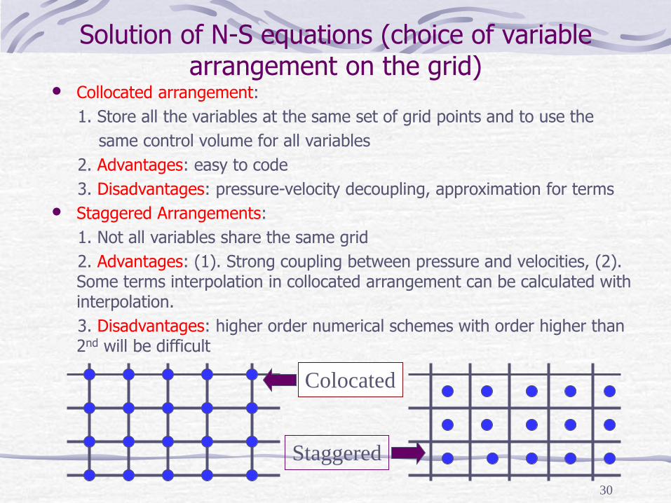
Solution of N-S equations (choice of variable arrangement on the grid)

• Collocated arrangement:

1. Store all the variables at the same set of grid points and to use the

same control volume for all variables

2. Advantages: easy to code

3. Disadvantages: pressure-velocity decoupling, approximation for terms

• Staggered Arrangements:

1. Not all variables share the same grid

2. Advantages: (1). Strong coupling between pressure and velocities, (2). Some terms interpolation in collocated arrangement can be calculated with interpolation.

3. Disadvantages: higher order numerical schemes with order higher than 2nd will be difficult

Colocated

Staggered

31

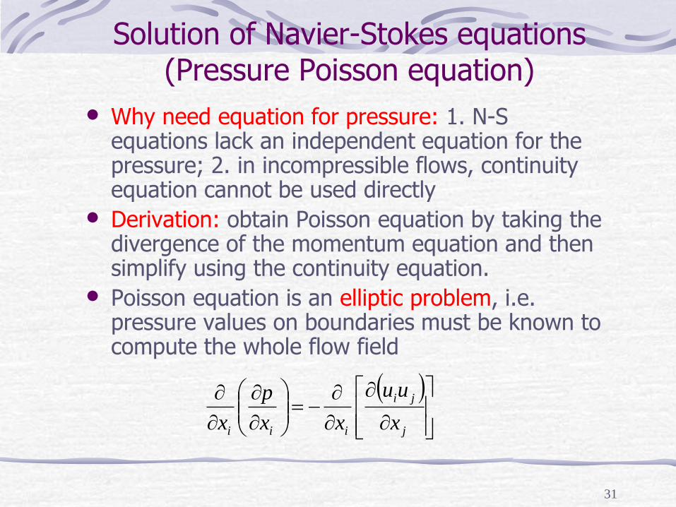
Solution of Navier-Stokes equations (Pressure Poisson equation)

• Why need equation for pressure: 1. N-S equations lack an independent equation for the pressure; 2. in incompressible flows, continuity equation cannot be used directly

• Derivation: obtain Poisson equation by taking the divergence of the momentum equation and then simplify using the continuity equation.

• Poisson equation is an elliptic problem, i.e. pressure values on boundaries must be known to compute the whole flow field

j

ji

iii x

uu

xx

p

x

32

Solution methods for the Navier-Stokes equations

• Analytical Solution (fully developed laminar pipe flow)

• Vorticity-Stream Function Approach: eliminate pressure term

• The SIMPLE (Semi-Implicit Method for pressure-Linked Equations) Algorithm:

1. Guess the pressure field p*

2. Solve the momentum equations to obtain u*,v*,w*

3. Solve the p’ equation (The pressure-correction equation)

4. p=p*+p’

5. Calculate u, v, w from their starred values using the

velocity-correction equations

6. Solve the discretization equation for other variables, such as

temperature, concentration, and turbulence quantities.

7. Treat the corrected pressure p as a new guessed pressure p*,

return to step 2, and repeat the whole procedure until a

converged solution is obtained.

33

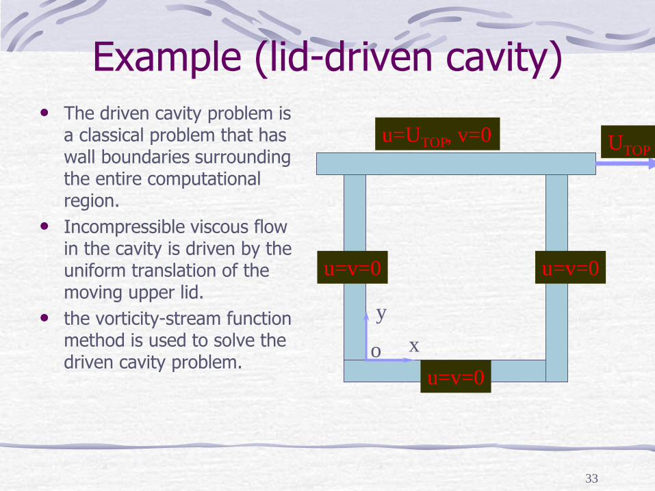
Example (lid-driven cavity)

• The driven cavity problem is a classical problem that has wall boundaries surrounding the entire computational region.

• Incompressible viscous flow in the cavity is driven by the uniform translation of the moving upper lid.

• the vorticity-stream function method is used to solve the driven cavity problem.

UTOP

o

y

x

u=v=0

u=v=0 u=v=0

u=UTOP, v=0

34

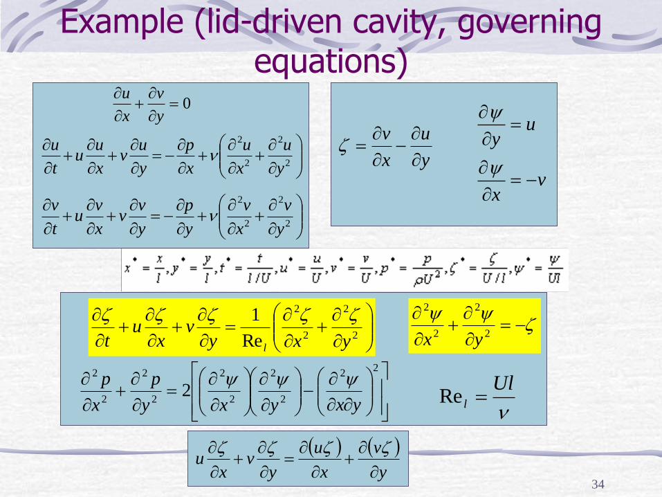
Example (lid-driven cavity, governing equations)

0

y

v

x

u

2

2

2

2

y

u

x

u

x

p

y

uv

x

uu

t

u

2

2

2

2

y

v

x

v

y

p

y

vv

x

vu

t

v

y

u

x

v

vx

uy

2

2

2

2

Re

1

yxyv

xu

t l

2

2

2

2

yx

2

2

2

2

2

2

2

2

2

2

2yxyxy

p

x

p

Ull Re

y

v

x

u

yv

xu

35

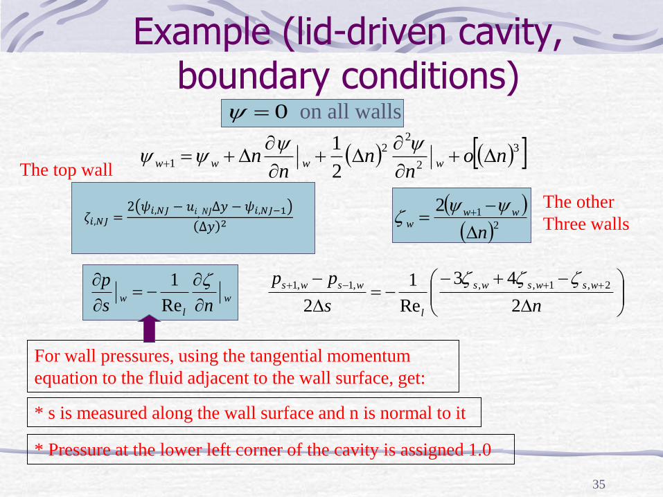
Example (lid-driven cavity, boundary conditions)

0 on all walls

3

2

22

12

1no

nn

nn wwww

𝜁𝑖,𝑁𝐽 =2 𝜓𝑖,𝑁𝐽 − 𝑢𝑖, 𝑁𝐽Δ𝑦 − 𝜓𝑖,𝑁𝐽−1

Δ𝑦 2

2

12

n

www

w

l

wns

p

Re

1

ns

pp wswsws

l

wsws

2

43

Re

1

2

2,1,,,1,1

The other

Three walls

The top wall

For wall pressures, using the tangential momentum

equation to the fluid adjacent to the wall surface, get:

* s is measured along the wall surface and n is normal to it

* Pressure at the lower left corner of the cavity is assigned 1.0

36

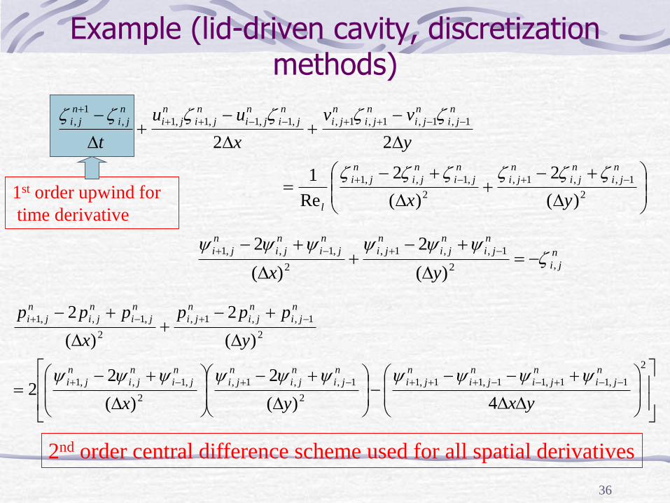
Example (lid-driven cavity, discretization methods)

2

1,,1,

2

,1,,1

1,1,1,1,,1,1,1,1,

1

,

)(

2

)(

2

Re

1

22

yx

y

vv

x

uu

t

n

ji

n

ji

n

ji

n

ji

n

ji

n

ji

l

n

ji

n

ji

n

ji

n

ji

n

ji

n

ji

n

ji

n

ji

n

ji

n

ji

n

ji

n

ji

n

ji

n

ji

n

ji

n

ji

n

ji

yx,2

1,,1,

2

,1,,1

)(

2

)(

2

2

1,11,11,11,1

2

1,,1,

2

,1,,1

2

1,,1,

2

,1,,1

4)(

2

)(

22

)(

2

)(

2

yxyx

y

ppp

x

ppp

n

ji

n

ji

n

ji

n

ji

n

ji

n

ji

n

ji

n

ji

n

ji

n

ji

n

ji

n

ji

n

ji

n

ji

n

ji

n

ji

2nd order central difference scheme used for all spatial derivatives

1st order upwind for

time derivative

37

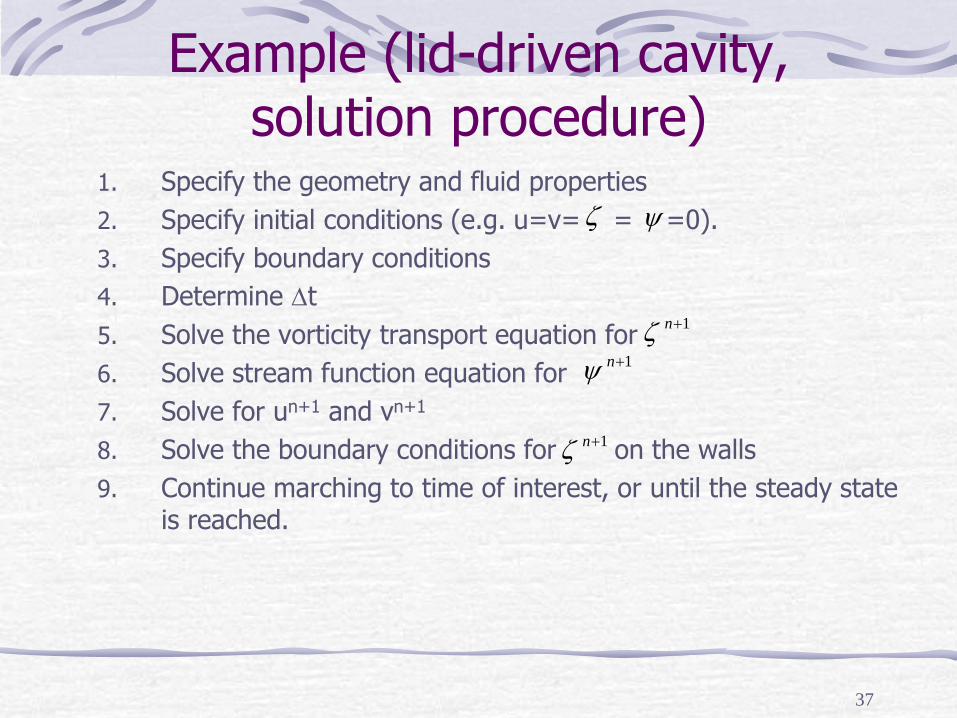
Example (lid-driven cavity, solution procedure)

1. Specify the geometry and fluid properties

2. Specify initial conditions (e.g. u=v= = =0).

3. Specify boundary conditions

4. Determine t

5. Solve the vorticity transport equation for

6. Solve stream function equation for

7. Solve for un+1 and vn+1

8. Solve the boundary conditions for on the walls

9. Continue marching to time of interest, or until the steady state is reached.

1n1n

1n

38

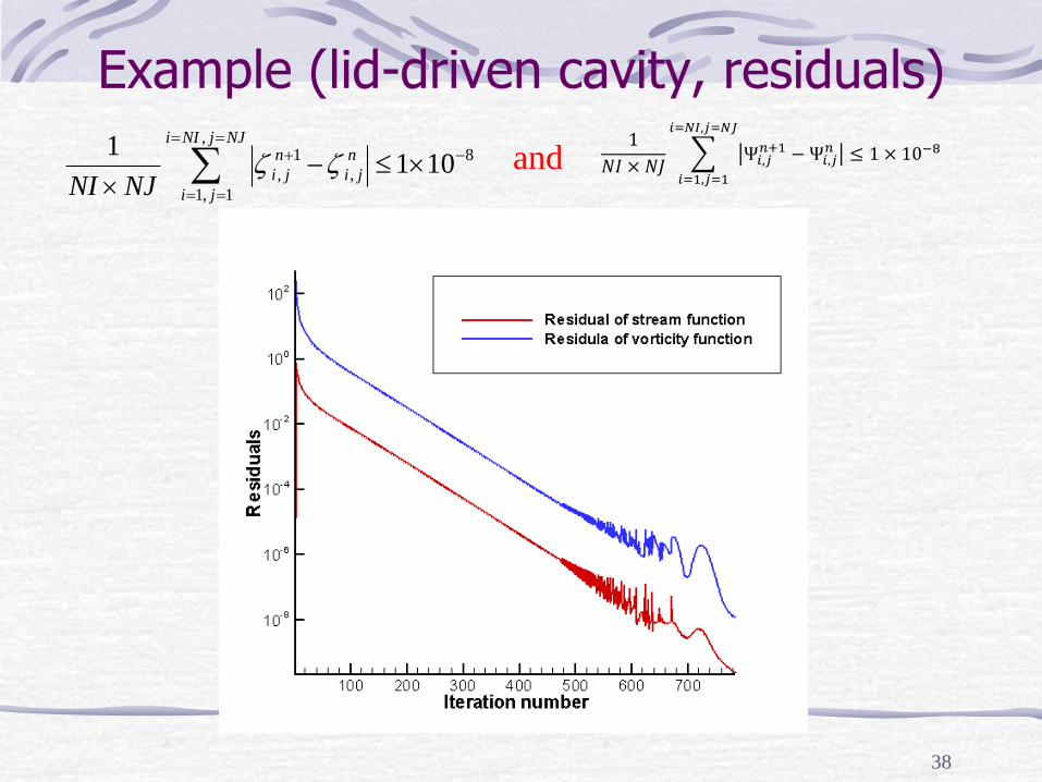
Example (lid-driven cavity, residuals)

8,

1,1

,

1

, 1011

NJjNIi

ji

n

ji

n

jiNJNI

1

𝑁𝐼 × 𝑁𝐽

𝑖=1,𝑗=1

𝑖=𝑁𝐼,𝑗=𝑁𝐽

Ψ𝑖,𝑗𝑛+1 −Ψ𝑖,𝑗

𝑛 ≤ 1 × 10−8and

39

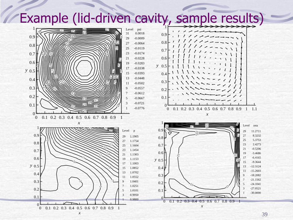
Example (lid-driven cavity, sample results)

3

3

5

5

7

7

7

9

9

9

9

11

11

11

11

13

13 13

13

13

15

1514

15

15

17

17

17

17

17

19

19

19

19

19

21

21

21

21

21

21

23

23

23

23

23

23

25

25

25 23

25

25

25

27

27

27 27

27

27

27

28

29

2929

29

29

29

29

0 0.1 0.2 0.3 0.4 0.5 0.6 0.7 0.8 0.9 10

0.1

0.2

0.3

0.4

0.5

0.6

0.7

0.8

0.9

1 Level psi

31 0.0018

29 -0.0009

27 -0.0064

25 -0.0119

23 -0.0174

21 -0.0228

19 -0.0283

17 -0.0338

15 -0.0393

13 -0.0448

11 -0.0502

9 -0.0557

7 -0.0612

5 -0.0667

3 -0.0721

1 -0.0776

y

x

0 0.1 0.2 0.3 0.4 0.5 0.6 0.7 0.8 0.9 1 1.10

0.1

0.2

0.3

0.4

0.5

0.6

0.7

0.8

0.9

1

y

x

3

5

5

5

7

7

7

9

9

11

11

13

13

15

15 17

17

19

19

21 2325

27 29

0 0.1 0.2 0.3 0.4 0.5 0.6 0.7 0.8 0.9 10

0.1

0.2

0.3

0.4

0.5

0.6

0.7

0.8

0.9

1Level p

29 1.1905

27 1.1754

25 1.1604

23 1.1454

21 1.1303

19 1.1153

17 1.1003

15 1.0852

13 1.0702

11 1.0552

9 1.0401

7 1.0251

5 1.0101

3 0.9950

1 0.9800

y

x

4911 814 1316 1517 1719 19

19

21

2121

21

2121

21

23

24

23

25

25

25

27

27

29

0 0.1 0.2 0.3 0.4 0.5 0.6 0.7 0.8 0.9 10

0.1

0.2

0.3

0.4

0.5

0.6

0.7

0.8

0.9

1Level zeta

29 11.2711

27 8.3232

25 5.3753

23 2.4273

21 -0.5206

19 -3.4686

17 -6.4165

15 -9.3644

13 -12.3124

11 -15.2603

9 -18.2082

7 -21.1562

5 -24.1041

3 -27.0521

1 -30.0000

y

x

40

Some good books

1. J. H. Ferziger, M. Peric, “ Computational Methods for Fluid

Dynamics,” 3rd edition, Springer, 2002.

2. Patric J. Roache, “Verification and Validation in

Computational Science and Engineering,” Hermosa

publishers, 1998

3. Frank, M. White, “Viscous Fluid Flow,” 3rd edition,

McGraw-Hill Inc., 2006