numerical modeling of coastline evolution in an era of global
TRANSCRIPT
i
v
NUMERICAL MODELING OF COASTLINE EVOLUTION IN AN ERA OF GLOBAL CHANGE
by
Jordan Matthew Slott
Division of Earth and Ocean Sciences Duke University
Date:_______________________ Approved:
___________________________
A. Brad Murray, Supervisor
___________________________ Peter K. Haff
___________________________
Lincoln Pratson
___________________________ Martin D. Smith
Dissertation submitted in partial fulfillment of the requirements for the degree of Doctor
of Philosophy in the Department of Earth and Ocean Sciences in the Graduate School
of Duke University
2008

ABSTRACT
NUMERICAL MODELING OF COASTLINE EVOLUTION IN AN ERA OF GLOBAL CHANGE
by
Jordan Matthew Slott
Division of Earth and Ocean Sciences Duke University
Date:_______________________ Approved:
___________________________
A. Brad Murray, Supervisor
___________________________ Peter K. Haff
___________________________
Lincoln Pratson
___________________________ Martin D. Smith
An abstract of a dissertation submitted in partial fulfillment of the requirements for the degree
of Doctor of Philosophy in the Department of Earth and Ocean Sciences in the Graduate School
of Duke University
2008

Copyright by Jordan Matthew Slott
2008

iv
Abstract
Scientists expect temperatures on Earth to get substantially warmer over the
course of the 21st century, causing storm systems to intensify and sea-level rise to
accelerate--these changes will likely have dramatic impacts on how the coastlines of
tomorrow will evolve. Humans are also playing an increasingly important role in
shaping Earth’s coastal systems. Coastal scientists have only a general understanding of
how these three factors—humans, storms, and sea-level rise—will alter the evolution of
coastlines over the coming century, however. I conduct numerical modeling experiments
to shed light on the relative importance of these factors on the evolution of coastline
geomorphology.
In a series of experiments using a numerical model of large-scale (1 to 100’s km)
and long-term (years to centuries) coastline evolution that results from gradients in
alongshore sediment transport, I explore how the patterns and rates of shoreline erosion
and accretion are affected by shifts in ‘wave climate’ (the mix of influences on
alongshore sediment transport of waves approaching from different directions) induced
by intensified storm systems and the direct manipulation of the shoreline system by
humans through beach nourishment (periodically placing sand on an eroding beach). I
use a cuspate-cape coastline, similar to the Outer Banks, North and South Carolina,
USA, as an important case study in my experiments. I observe that moderate shifts in
the wave climate can alter the patterns of shoreline erosion and accretion, potentially
increasing migration rates by several times that which we see today, and nearly an
order-of-magnitude larger than sea-level rise-related erosion alone. I also find that under

v
possible wave climate futures, beach nourishment may also induce shoreline change on
the same order of magnitude as does sea-level rise.
The decision humans make whether or not to nourish their beach often depends
upon a favorable economic outcome in the endeavor. In further experiments, I couple a
cost-benefit economic model of human decision making to the numerical model of
coastline evolution and test a hypothetical scenario where two communities (one ‘rich’
and one ‘poor’) nourish their beaches in tandem, under different sets of economic and
wave climate parameters. I observe that two adjacent communities can benefit
substantially from each other’s nourishment activity, and these effects persist even if the
two communities are separated by several tens of kilometers.
In a separate effort, I employ techniques from dynamic capital theory coupled to
a physically-realistic model of coastline evolution to find the optimum time a community
should wait between beach nourishment episodes (‘rotation length’) to maximize the
utility to beachfront property owners. In a series of experiments, I explore the sensitivity
of the rotation length to economic parameters, including the discount rate, the fixed and
variable costs of beach nourishment, and the benefits from beach nourishment, and
physical parameters including the background erosion rate and the exponential rate at
which both the cross-shore profile and the plan-view coastline shape re-adjusts
following a beach nourishment episode (‘decay rate’ of nourishment sand). Some results
I obtained were expected: if property values, the hedonic value of beach width, the
baseline retreat rate, the fixed cost of beach nourishment, and the discount rate increase,
then the rotation length of nourishment decreases. Some results I obtained, however,
were unexpected: the rotation length of nourishment can either increase or decrease when
the decay rate of nourishment sand varies versus the discount rate and when the
variable costs of beach nourishment increase.

vi
Acknowledgements
Undertaking this doctoral research has been perhaps the most complex and
arduous, yet rewarding, tasks of my professional life. I could not have accomplished this
research if it not were for the support of Duke University and the Nicholas School of the
Environment and Earth Sciences and the dedication of the faculty of the Division of
Earth and Ocean Sciences.
Foremost, I am deeply indebted to my advisor, Professor A. Brad Murray at the
Division of Earth and Ocean Sciences, Nicholas School of the Environment and Earth
Sciences, Duke University for his guidance, tutelage, and mentorship over these past five
years. He took me in as a graduate student in Fall 2003 entirely unschooled in earth
science, geology, and nearshore morphodynamics. He counseled me through years of
independent study and frequent meetings to discuss, plan, and execute upon research
ideas. I am proud to co-author all of my papers with him; his editorial assistance was
invaluable.
I would also like to thank Professor Martin D. Smith at the Division of
Environmental Science and Policy, Nicholas School of the Environment and Earth
Sciences, Duke University. My work coupling economic models to numerical models of
coastline evolution comes from my collaboration with Marty. He is responsible for
everything I know about natural resource economics.
I am also grateful to Professors Peter K. Haff and Lincoln Pratson who served on
my doctoral committee, contributed to my earth science education, and provided
valuable feedback on my research. My research was financially supported by the Duke
University Graduate School, the Duke Center on Global Change and the National
Science Foundation. The research I present here reflects one part of a larger project

vii
funded by the NSF and I am grateful to my fellow researchers Professor Michael Orbach,
Professor Joseph Ramus, Dylan McNamara, and Sathya Gopalakrishnan.
Several faculty members of the Division of Earth and Ocean Sciences have served
as informal mentors during the course of my doctoral work. I am grateful to Professor
Susan Lozier, Chair, Division of Earth and Ocean Sciences for the endless discussions
we have had on graduate school, teaching, and life. This work, in part, builds upon the
efforts of current and previous graduate students in the Division of Earth and Ocean
Sciences. I thank them for their contributions and help: Andrew D. Ashton, Lisa M.
Valvo, Eli Lazarus, Matthew L. Kirwan, and Ryan Littlewood.

viii
Contents
Abstract ............................................................................................................................................... iv
Acknowledgements ...........................................................................................................................vi
List of Tables...................................................................................................................................... xi
List of Figures ....................................................................................................................................xii
1. Introduction..................................................................................................................................... 1
2. Coastline responses to changing storm patterns..................................................................... 5
2.1 Introduction............................................................................................................................ 5
2.2 Methods .................................................................................................................................. 7
2.2.1 Numerical Model ............................................................................................................. 7
2.2.2 Representing the Recent Wave Climate ...................................................................... 9
2.2.3 Initial Conditions for Model Experiments ...............................................................12
2.2.4 Representing the Influence of Varying Storm Activity ..........................................12
2.3 Results ...................................................................................................................................15
2.4 Discussion ............................................................................................................................17
3. Responses of Complex-Shaped Coastlines to Beach ‘Nourishment’ and Climate Change.................................................................................................................................................20
3.1 Introduction..........................................................................................................................20
3.2 Background...........................................................................................................................23
3.2.1 One-contour-line Numerical Modeling......................................................................23
3.2.2 High-Wave-Angle Instability ......................................................................................24
3.2.3 Sensitivity of a Cuspate-Cape System to Shifting Wave Climates....................27
3.2.4 Modeling Beach Nourishment.....................................................................................28
3.3 Methods ................................................................................................................................29
3.3.1 Numerical Model ...........................................................................................................29

ix
3.3.2 Model Experiments .......................................................................................................30
3.3.3 Wave Climates Used in Model Experiments ..........................................................31
3.3.4 Initial Cuspate-Cape Model Shoreline......................................................................33
3.3.5 Beach Nourishment .......................................................................................................34
3.4 Results ...................................................................................................................................35
3.4.1 Nourishment of a Flat Shoreline.................................................................................35
3.4.2 Nourishment on a Cuspate-Cape Shoreline ............................................................37
3.4.3 Increased Extra-Tropical Storminess ........................................................................40
3.4.4 Increased Extra-Tropical Storminess and Beach Nourishment ..........................43
3.4.5 Beach Nourishment Under Other Wave Climate-Change Scenarios .................45
3.4.6 Beach Nourishment Sand Volumes ...........................................................................46
3.4.7 Interpretation of Physical Mechanisms ....................................................................48
3.5 Discussion ............................................................................................................................53
3.5.1 Sea Level Rise.................................................................................................................53
3.5.2 Sensitivity to Model Parameters................................................................................54
3.5.3 Model Simplifications ..................................................................................................56
3.6 Conclusion............................................................................................................................59
4. Synergies Between Adjacent Beach-Nourishing Communities in a Morpho-economic Coupled Coastline Model...............................................................................................................60
4.1 Introduction..........................................................................................................................60
4.2 Background...........................................................................................................................61
4.2.1 Numerical Models of Coastline Evolution...............................................................61
4.2.2 Economic Models of Beach Nourishment ................................................................64
4.3 Methods ................................................................................................................................66
4.3.1 Numerical Model of Coastline Change.....................................................................66
x
4.3.2 Beach Nourishment .......................................................................................................69
4.3.3 Cost-Benefit Economic Model ....................................................................................70
4.3.4 Model Experiments .......................................................................................................73
4.4 Results ...................................................................................................................................75
4.4.1 Varying Wave Climates ...............................................................................................75
4.4.2. Varying Distance Separating Communities............................................................80
4.4.3 Increased Nourishment Costs .....................................................................................81
4.5 Discussion and Conclusion...............................................................................................83
5. Beach nourishment as a dynamic capital accumulation problem.....................................87
5.1 Background...........................................................................................................................88
5.2 The Model.............................................................................................................................92
5.3 Comparative Statics of Beach Nourishment Rotations............................................100
5.4 Discussion ..........................................................................................................................114
References.........................................................................................................................................117
Biography .........................................................................................................................................125

xi
List of Tables
Table 1. Sensitivity of model results to beach nourishment interval, I .................................55
Table 2. Sensitivity of model results to beach nourishment length, L...................................56

xii
List of Figures
Figure 1: The coastline of North and South Carolina, from Cape Hatteras, NC to Cape Fear, SC, USA ..................................................................................................................................... 7
Figure 2: Schematic illustration of gradients in the magnitude of alongshore sediment flux................................................................................................................................................................ 9
Figure 3: Coastline response to various wave climates............................................................11
Figure 4: Contour plots of shoreline-change and erosion rates (meters/year) for different combinations of wave climate parameters A and U ................................................................16
Figure 5. The coastline of North and South Carolina, from Cape Hatteras, NC to Cape Fear, SC, USA ...................................................................................................................................22
Figure 6. ‘One-contour-line’ modeling approach .......................................................................24
Figure 7. Schematic illustration of zones of shoreline erosion and accretion caused by gradients in the alongshore sediment flux, Qs. ...........................................................................25
Figure 8. Evolution of a flat shoreline in response to repeated beach nourishment over 200 years under an imposed baseline erosion rate of 1 m/yr. ...............................................36
Figure 9. Evolution of a cuspate-cape shoreline in response to repeated beach nourishment over 200 years for six different site selections, subjected to a wave climate approximating recent conditions off of the Carolina coast, USA (WIS) .............................38
Figure 10. Cumulative beach nourishment volume (m3) for model runs presented in Figure 9. ...........................................................................................................................................................40
Figure 11. Shoreline response to increased extra-tropical storm influence and a 10 km beach nourishment............................................................................................................................42
Figure 12. Contour plots of nourishment-caused components of shoreline change rates within 10 km and 20 km of a beach nourishment .....................................................................46
Figure 13. Beach nourishment sand volumes for different combinations of wave climate parameters A and U ........................................................................................................................47
Figure 14. Definition sketch of model run statistics Q’net, the flux perturbation, and Q’shadow, the extent to which wave shadowing was responsible for Q’net. ...........................50
Figure 15. Physical mechanisms of human-induced shoreline change ..................................51
Figure 16: Schematic illustration of zones of shoreline change caused by the relative wave angle along a curving coastline.......................................................................................................64

xiii
Figure 17: ‘One-contour-line’ modeling approach .....................................................................67
Figure 18: Coupling a numerical and economic model of beach nourishment in plan view.........73
Figure 19: Beach nourishment experiments involving both “poor” and “rich” communities, in plan view ..............................................................................................................................................74
Figure 20: Shoreline position for one and two nourishing communities over 200 years, in plan view ......................................................................................................................................................76
Figure 21: Contour plot of total undiscounted costs of beach nourishment experiments from Figure 19, for thirty-six combinations of wave climate parameters, A and U ................................78
Figure 22: Total undiscounted costs of beach nourishment for “poor” and “rich” communities when they exist together and separated by varying distances, ranging from 5 km to 50 km .........81
Figure 23: Total undiscounted costs of beach nourishment (solid line) and average property value (dotted line) for “poor” and “rich” communities when they exist together, as the federal share of nourishment costs decreases ...............................................................................................................83
Figure 24. Cross- and along-shore response of the coastline to beach nourishment .........91
Figure 25. Beach width on a 10-year rotation............................................................................97
Figure 26. Sand use patterns with and without nourishment decay.....................................98
Figure 27. Increasing variable cost of sand can accelerate or decelerate nourishment....107
Figure 28. A higher value of beach width increases the frequency of nourishment..........108
Figure 29. A higher base property value increases the frequency of nourishment ...........109
Figure 30. A higher baseline erosion rate increases the frequency of nourishment...........110
Figure 31. Frequency of nourishment increases with a higher share of beach width subject to exponential decay......................................................................................................................111
Figure 32. A higher exponential decay of nourishment sand increases (decreases) frequency of nourishment if the decay rate is lower (higher) than the discount rate ......113

1
1. Introduction
Global warming of the atmosphere and oceans expected during the coming century
will likely have dramatic impacts on the world’s coastal areas: scientists expect sea level
to rise roughly 0.5 meters (IPCC 2007) and storm systems (e.g. Atlantic tropical and
Northern hemisphere extra-tropical cyclones) to intensify (Emanuel 1987, 2003; Lambert
1995). Humans will also play a direct role in the evolution of our coastlines, by
attempting to stabilize the position of shorelines to combat erosion and protect valuable
homes, roads, and other infrastructure. This dissertation addresses for the first time the
relative importance of these three factors—sea-level rise, intensified storms, and direct
human actions—on the evolution of a large-scale coastline system.
In Chapter 2, I utilize a numerical model of coastline evolution to explore how
intensified storm systems alter the patterns and rates of shoreline erosion and accretion
(Slott et al. 2006). The numerical model (Ashton, Murray, and Arnoult 2001; Ashton
and Murray 2006a,b) treats coastline evolution over large spatial scales (1 to 100’s km)
and long time scales (years to centuries) that result from gradients in wave-driven
alongshore sediment transport. It has previously been used to illustrate how complex-
shaped coastlines (e.g. cuspate-capes, spits) self-organize over millennia, where
alongshore sediment transport induces instabilities in the shoreline shape and causes
plan-view perturbations to grow seaward. The coastline shape itself is a function of the
relative influences on alongshore sediment transport of waves approaching from
different directions regionally (the directional ‘wave climate’). As plan-view
perturbations grow larger, they interact with one another over surprisingly large
distances through ‘wave shadowing’—protruding shoreline features block waves from
2
reaching other parts of the coast, altering the local wave climate and therefore evolution
of the shoreline there.
I use the Outer Banks of North and South Carolina, USA as a case study--its 100
km-scale cuspate-cape shape presumably exists in quasi-equilibrium with current
regional wave climate conditions that have shifted the capes to the Southwest at ~3
m/yr over the past half-century. I explore how moderate shifts in the regional wave
climate—one possible outcome of the intensification of storms we expect over the
coming century (Emanuel 1987, 2005)—can result in dramatic shifts in the patterns of
erosion and accretion along the shoreline (Slott et al. 2006). Chapter 2 was published in
Geophysical Research Letters in 2006 with co-authors A. Brad Murray, Andrew D.
Ashton, and Thomas J. Crowley.
In the model results presented in Chapter 2, the shoreline is free to erode or accrete
everywhere as a result of the wave climate forcing. These numerical modeling results,
where the shoreline evolves freely, are not pertinent to the many human-developed
shorelines of today, however. Few shorelines can be considered ‘pristine’ as humans
frequently employ some means of stabilizing the position of the shoreline to protect
valuable infrastructure from erosion. The direct actions humans take will likely
significantly alter shoreline evolution in the long run—this hypothesis is motivated by the
observation from previous results that on complex-shaped coastlines, the effects of
changes in one location may propagate over large distances quickly through non-local
mechanisms such as wave shadowing.
In Chapter 3, I couple direct human manipulations of the coastline system into the
numerical model, using beach nourishment (periodically placing sand on an eroding
beach to restore its original width) as the primary shoreline-stabilization method, and
conduct a series of experiments to test the sensitivity of coastline evolution to beach

3
nourishment, and any large-scale effects that may result, under a set of future wave
climates that might result from climate change. Chapter 3 represents a manuscript in
revision at Journal of Geophysical Research – Earth Surface with co-authors A. Brad
Murray and Andrew D. Ashton.
Unlike the model experiments presented in Chapter 3, beach nourishment rarely
occurs on a fixed, periodic schedule (Valverde, Trembanis, and Pilkey 1999). Rather,
communities nourish their beach according to an often complex set of conditions--e.g. to
prevent homes from falling into the sea or to enhance the recreational or storm protection
value of the beach--and may depend upon the availability of state and federal funding.
In many cases (e.g. USACE (2002)), the decision to nourish depends upon whether the
economic benefit of nourishment (e.g. storm protection and recreation) outweighs the
economic costs (e.g. dredging sand).
In Chapter 4, I present results from numerical modeling experiments where I
couple a cost-benefit economic decision-making model to the beach nourishment-enabled
model of large-scale coastline evolution. In these experiments, I test a hypothetical
scenario where a ‘rich’ community exists next to a ‘poor’ community and both nourish
their beach based upon a different set of economic parameters. In these experiments, I
vary both the wave climate and the economic parameters and report on how the
synergistic effects of two communities nourishing in tandem are affected by each.
Chapter 4 is a paper in press at Coastal Management Journal with co-authors Martin D.
Smith and A. Brad Murray.
In Chapter 5, I consider a question related to the work presented in Chapter 4: what
is the optimal time period a community should wait between re-nourishment episodes to
maximize the net economic benefits they receive from nourishment? I frame this question
in the context of a dynamic capital accumulation problem, similar to one used in the
4
forestry literature, by considering beach width to be natural resource ‘stock’ that
provides value to beach property owners and depreciates over time (from erosion).
Benefits to beach property owners come from storm protection and recreational benefits,
characterized as an amenity flow from the properties. I treat the coastline response to
beach nourishment in a physically accurate way: because beach nourishment disturbs the
cross-shore equilibrium profile and creates a plan-view ‘bump’ in the shoreline shape ,
sand from nourishment diffuses both seaward (to restore the cross-shore equilibrium
profile) and laterally (to diffusive the shoreline ‘bump’) at a rate that decreases
exponentially over time since the last re-nourishment episode (nourishment sand ‘rate of
decay’). I explore the effect of varying the economic (discount rate, fixed and variable
costs of nourishment, value of beach width) and physical (baseline erosion rate, sand
decay rate) parameters on the optimum length of time a community should wait before
re-nourishing their beach. The work in Chapter 5 represents a manuscript in revision at
the Journal of Environmental Economics and Management by lead author Martin D.
Smith. As part of my contributions as second author, I helped define the proper
representation of physical coastal processes to include in the mathematical model,
helped develop the numerical implementation of the model, contributed to the literature
review and model description in the manuscript, and provided assistance responding to
anonymous reviewers.

5
2. Coastline responses to changing storm patterns
2.1 Introduction
This chapter originally appeared as Slott, Jordan, A. Brad Murray, Andrew D.
Ashton, and Thomas J. Crowley, Coastline responses to changing storm patterns,
Geophysical Research Letters, 33, L18404, doi:10.1029/2006GL027445, 2006.
Reproduced by permission of American Geophysical Union.
Warming of the atmosphere and oceans expected in coming decades (IPCC 2007)
will likely cause storm behavior to change. Although changes in storminess cannot
currently be predicted with complete confidence, there is good reason to expect some
change in extra-tropical and tropical cyclone frequency and severity (Emanuel 1987,
2005; Lambert 1995; Geng and Sugi 2003; Webster et al. 2005). (Recent work suggests
that the total energy dissipated by tropical storms from meteorological records has
doubled over the past 30 years, and furthermore, is well-correlated with the observed
0.5ºC rise in SSTs (Emanuel 2005)). Shifts in storm behavior will alter the relative
amounts of wave energy approaching a shore from different directions (the ‘wave
climate’). Previous studies using a numerical model of coastline change on a large spatial
domain (Ashton, Murray, and Arnoult 2001; Ashton and Murray 2006a,b) have shown
that distinct plan-view shoreline shapes (e.g. cusps, spits) can emerge and evolve under
different wave climates. Therefore, if storm patterns and wave distributions change,

6
coastline shapes will tend to adjust—a process involving greatly accelerated shoreline
erosion in many areas that would affect coastal communities and infrastructure.
Shoreline changes from sea-level rise have received considerable attention
(Anderson et al. 2001; Brown et al. 2005; Bruun 1962; Cowell, Roy, and Jones 1995;
Gornitz 1991; Titus et al. 1991; U.S. Climate Change Science Program 2001; Zhang,
Douglas, and Leatherman 2000, 2004). Many studies assume that on sandy coastlines,
sea-level rise causes cross-shore sediment redistribution that leads to a landward
translation of the shoreline (Bruun 1962; Cowell, Roy, and Jones 1995; Zhang, Douglas,
and Leatherman 2000, 2004). Under this conceptual framework, shorelines will retreat in
a roughly alongshore-uniform manner in response to global warming. In contrast, we
evaluate here the heterogeneous nature of shoreline retreat related to changing storm
patterns on time scales of decades to centuries.
We use a numerical model to explore how a rapid change in wave climate will
affect a cuspate coastline shape, similar to the shape of the Carolina Capes, from Cape
Hatteras, NC to Cape Fear, SC, USA (Figure 1). This region of coastline serves as an
important and illustrative case study. Many parts of the Carolina Capes are heavily
developed and economically important; accelerated rates of shoreline migration will
further threaten homes and businesses built near the shoreline there today (Pilkey et al.
1998). We conducted two sets of model experiments, and in each compare coastline
changes under altered wave climates with coastline changes under the current wave
climate off of the US East Coast. In the first set, we select several representative wave
climate-change scenarios, based on an estimate of how storminess might change in the

7
future. In the second set of model experiments, we test a wide a range of possible future
wave climates.
Figure 1: The coastline of North and South Carolina, from Cape Hatteras, NC to Cape Fear, SC, USA along the US Atlantic coastline. From Ashton and Murray
(2006b).
2.2 Methods
2.2.1 Numerical Model
We first briefly discuss the model we use for this evaluation, which has been
described previously (Ashton, Murray, and Arnoult 2001). When waves break at a
shoreline, they drive a flux of sediment along the shore. The magnitude of this flux is
related to the breaking-wave height, and to the wave approach angle, relative to the
shoreline orientation (Figure 2). Alongshore sediment fluxes, Qs, are based on the
commonly used CERC equation (Komar and Inman 1970; Komar 1998, 390-3):
!
Qs = K1Hb
5 / 2sin("b #$)cos("b #$) (1)

8
where Hb and φb are breaking-wave height and crest angle, respectively, θ is local
shoreline orientation, and K1 is an empirical constant equal to 0.4 m1/2/s.
On a sandy coastline, alongshore gradients in this sediment flux, Qs, tend to
cause changes in the shoreline position, η (Figure 2):
!
"#
"t= $
1
D
"Qs
"x (2)
where D is the seabed depth to which erosion or accumulation extends. Large-
scale (> km) bends in a shoreline cause gradients in alongshore flux that alter the
shoreline shape. When waves approach from nearly straight offshore (as measured in
deep-water, before nearshore refraction), gradients in alongshore transport cause the
large-scale shoreline shape to become smoother (Figure 2a). However, when waves
approach from deep-water angles greater than approximately 45° (‘high-angle’ waves,
greater than the deep-water angle at which alongshore sediment transport is
maximized), plan-view shoreline undulations grow (Ashton, Murray, and Arnoult 2001)
(Figure 2b). Where high-angle waves dominate regional wave climates, complex coastline
shapes and behaviors arise (Ashton, Murray, and Arnoult 2001). In a recently
developed numerical model based on Equations 1 and 2 different shapes including
cuspate capes and spits evolve under different wave distributions (characterized by the
proportions of high-angle versus low-angle waves, and by the degree of asymmetry—the
proportion of wave influence from the left versus right, looking offshore) (Ashton,
Murray, and Arnoult 2001).

9
Figure 2: Schematic illustration of gradients in the magnitude of alongshore sediment flux, shown by the length of the arrows, caused by changes in shoreline orientation, and the consequent zones of erosion and accretion. a, Erosion and the
subsequent landward retreat of the plan-view ‘bump’ occurs under the influence of low-angle waves. b, Accretion and the subsequent seaward build-out of the plan-
view ‘bump’ occurs under the influence of high-angle waves.
The model domain is discretized into cells, and shoreline changes are determined
by a discretized form of Equation 2. Where protruding shoreline features block other
coastline segments from the current deep-water wave-approach angle, no sediment
transport occurs in the ‘shadowed’ segments. A new deep-water wave angle is chosen
daily from a probability distribution function (PDF) that represents a wave climate.
Breaking-wave height and angle relative to local shoreline orientations are calculated
assuming refraction and shoaling over shore-parallel contours.
2.2.2 Representing the Recent Wave Climate
We use twenty years of wave hindcasts off of the North Carolina coast, USA
(station 509) (WIS data can be found at http://frf.usace.army.mil/wis/, hereafter WIS)
as our ‘constant’ wave climate representing recent conditions. We form the wave climate
model input PDF from the wave hindcasts as follows. First, we rewrite the alongshore
sediment transport formula (Equation 1) above in terms of deep-water wave heights and

10
angles by assuming that waves shoal and refract over shore-parallel contours (Ashton,
Murray, and Arnoult 2001):
!
Qs
= K2H0
12 / 5sin("0 #$)cos
6 / 5("0 #$) (3)
where H0 is the deep-water wave height, φ0 is the deep-water wave approach
angle, and K2 is an empirical constant equal to 0.32 m3/5s-6/5. The influence a deep-water
wave has on alongshore sediment transport, therefore, scales with the 12/5th power of
its wave height. Next, we scale each wave height from the wave hindcasts (WIS)
accordingly before being added to the wave approach angle PDF. We fit two
parameters, A and U, to the PDF (e.g. Figure 3). The dimensionless wave-asymmetry
parameter, A, describes the proportion of wave influences approaching from the left
(looking off-shore); the dimensionless wave-angle highness parameter, U, describes the
proportion of wave influences approaching from high-angles (> ~ 45°). (Together, they
describe four probability bins: from-the-left and high-angle, from-the-left and low-angle,
from-the-right and low-angle, and from-the-right and high-angle.) Deep-water significant
wave height is held constant at 1.7 m throughout each simulation, based on
!
< H0
12 / 5>5 /12
for the hindcast data (WIS)—the effective average wave height for calculating net
alongshore sediment transport.

11
Figure 3: Plan-view shorelines. a, The Carolina capes rotated counterclockwise 150 degrees so that the regional offshore direction is up, with a depiction of the regional
wave climate (inset) showing relative wave influence from each 7.5° angle bin (Ashton and Murray 2006a,b). b, Model shoreline shape produced using wave-
climate parameters based on WIS station 509 off of North Carolina, USA (WIS): The proportion of high-angle waves, U, = 0.60; the proportions of waves from the left, A,
= 0.55, and average deep-water wave height = 1.7m. The model wave climate is depicted by the blue bin outlines in the histogram. Also shown are the shoreline
changes occurring over 200 years with this same wave climate; red indicates shoreline erosions, and green indicates accretion. The alongshore average of the magnitude of shoreline-change rates is denoted by |r|, the alongshore-averaged
erosion (accretion) rates within eroding (accreting) shoreline segments are denoted by e (a). Shoreline change is also depicted graphically. c, Initial coastline as in b, modified over 200 years by a wave climate with U, = 0.70 and A, = 0.45. d, Initial
coastline as in b, modified over 200 years by a wave climate with U, = 0.70 and A, = 0.65. e, Initial coastline as in b, modified over 200 years by a wave climate with U, =
0.50 and A, = 0.55. Satellite image courtesy of the SeaWiFS Project NASA/GSFC and ORBIMAGE.

12
2.2.3 Initial Conditions for Model Experiments
To produce the initial coastline for model experiments (Figure 3b), we based the
model wave climate roughly on the 20 years of wave hindcast off of the Carolina coast
(WIS), and beginning with a straight shoreline (plus white-noise perturbations), let the
model run for approximately 8000 simulated years. We treat this simulated coastline as
a representative example of a cuspate coast, rather than attempting to model the
evolution and morphology of the Carolina coastline in detail. (The Holocene
development of the Carolina Capes likely started with large-scale undulations in the
inherited coastline, requiring less time than the evolution from an approximately straight
coast in the model. In addition, wave climates have not likely been constant for
millennia. We assume only that over recent centuries wave climates have been steady
enough for such coastline shapes to attain a quasi-equilibrium.)
Mid-latitude winter storms off of the US East Coast (‘Noreasters’) produce
waves that tend to approach from the northeast at high-angles relative to the trend of
the Carolina coastline, whereas Atlantic tropical storms produce waves from the south.
These two storm influences combine to produce a regional wave climate dominated by
high-angle waves, as well as a moderate asymmetry (net transport would be to the
southwest along a straight coastline with the overall trend of the Carolina Capes, Figure
1).
2.2.4 Representing the Influence of Varying Storm Activity
Precisely how tropical storms, extra-tropical storms, and prevailing winds will
change as the climate warms remains unknown. Thus, we will present a range of
scenarios involving changes in storm activity relative to the background onshore winds.

13
To estimate a reasonable magnitude for changes in the model wave-climate parameters,
we start with Emanuel’s (1987) prediction that tropical-storm wind speeds will increase
by 10% given a 2° SST increase. Relating storm size and frequency to increased SSTs
remains elusive, however. Although we can reasonably expect that global warming will
lead to changes in storm frequency, duration, and size, we only consider a 10% increase
in storm wind speed (Emanuel 1987) as both a simplifying assumption and conservative
estimate of change.
An index of the shear stress exerted on the water surface by wind, ua (m/s), is a
non-linear function of the wind speed, u (m/s) (Komar 1998, 153-4):
!
ua
=1.7u1.23 (4)
Empirical measurements show that in situations where the distance over which
the wind blows (fetch) limits the growth of the waves, wave heights scale linearly with
ua. However, if the fetch does not limit the growth of the waves, wave heights scale
quadratically with ua. If we increase the wind speed, u, by 10% these empirical
relationships suggest wave height increases between ~12% (fetch-limited) and ~26%
(fully-developed waves) (Komar 1998, 153-4). In lieu of a fetch analysis of storm winds,
we chose a 12% (fetch-limited) increase in wave heights as a conservative estimate.
Using the 12/5th scaling relationship between deep-water wave height and alongshore
sediment transport, a ~12% increase in the deep-water wave height (fetch-limited)
results in an approximately 32% increase in alongshore sediment transport.
For our Carolina coastline case study (Figure 3), the vast majority of waves
generated by tropical storms approach the coast from the right (using a regionally-

14
averaged coastline orientation). The approximation that all tropical-storm derived
waves come from the right allows a simple calculation of a change in wave-climate
asymmetry, A, starting from the estimated wave climate for the last two decades of last
century (WIS), A = 0.55, U = 0.60.
If we let Influenceleft represent the influence on alongshore sediment transport
from left-approaching waves and Influenceright represent the influence from right-
approaching waves, the wave climate parameter, A, represents the proportion of left-
approaching wave influences:
!
A =Influenceleft
Influenceleft + Influenceright (5)
Inserting A = 0.55 into Equation 5, yields Influenceright = 0.82 Influenceleft. Holding
the influence from the left constant, and increasing the new Influenceright to 1.32(0.82)
Influenceleft (i.e. by 32%) leads to Anew = 0.48; a 12.7% change in the parameter value.
Given the conservative fetch-limitation assumption, changing A from 0.55 to 0.45 in the
increased tropical-storm wave-climate scenario described below (Figure 3c) seems
reasonable.
In this tropical-storm-change scenario (Figure 3c) we also change U, representing
the assumption that most of the tropical-storm derived waves approach the coast from
high angles, as tropical storms frequently propagate northward along the SE US
coastline, radiating waves toward the Carolina coastline from highly oblique angles.
According to the conservative analysis above (involving the fetch-limitation
assumption), an increase in U of 0.10, as in Figure 3c, is an overestimation of the effect,

15
because not all tropical-storm derived waves approach from high angles, and tropical
storms do not affect high-angle waves from the left.
Based on the simple analysis of changes in A from tropical-storm changes, we
use a 0.10 change in the wave climate statistics as an order-of-magnitude guide for the
remaining two wave climate scenarios presented below (Figures 3d-e).
2.3 Results
We conducted a sensitivity study to investigate the responses of a cuspate
coastline to climate change. Figure 3b shows the changes in the model coastline over 200
years of evolution under a constant wave climate; the large-scale coastline shape
changes relatively little on human timescales under these conditions, although continued
southwestward translation of the capes does cause shoreline changes of hundreds of
meters per century near the capes, consistent with historical observations (Fifty-year
historical shoreline data for North Carolina can be found at
http://dcm2.enr.state.nc.us/Maps/erosion.htm, hereafter NC50). Figure 3c shows how
the simulated coastline changes during 200 years of evolution under an altered wave
climate, which features a 10% greater proportion of high-angle waves, and a 10% lower
asymmetry (an increase in waves from the right). These changes along the Carolina
Capes would correspond to an increase in the relative influence of tropical-storm waves.
Figure 3d shows the effects of a 10% increase in the proportion of high-angle waves and
a 10% higher asymmetry (increase in waves from the left). For the Carolina coast, this
would correspond to an increase in the influence of extra-tropical winter storms. Figure
3e shows how the shoreline shape would change if the proportion of high angle waves
decreases (by 10%), which would occur along the Carolina Coast if the relative energy
from tropical and extra-tropical storms decreased. In the wave-climate-change

16
scenarios, areas of accretion as well as large areas of accelerated erosion result, with
alongshore-averaged shoreline change rates (including magnitudes of erosion and
accretion rates individually) several times those that occurred without the change in
wave climate. Maximum shoreline change rates in the climate-change scenarios (Figures
3c-e) approach an order of magnitude higher than the maximum rates with the
unchanged climate (Figure 3b).
Figure 4 shows how alongshore-averaged shoreline change and erosion rates in
the model depend on the magnitudes of changes in wave climate asymmetry and the
proportion of high-angle waves. The expected magnitude of changes in wave-climate
parameters depend on how storm patterns might change. As discussed above (Section
2.2.4), a consideration of expected changes in tropical storm characteristics provides
some guidance; a 10% increase in tropical storm wind speed would produce changes in
model wave-climate parameters of roughly 0.10. This suggests an envelope (Figure 4a,b,
dotted rectangle) within which illustrates the rates of shoreline change and erosion we
might conservatively expect over the coming decades to centuries.
Figure 4: Contour plots of shoreline-change and erosion rates (meters/year) for different combinations of wave climate parameters A and U, in experiments like
those described in Figure 3. The rates under an unchanged climate (A = 0.55, U = 0.60) are marked with small filled circles. a, Alongshore-averaged magnitude of

17
shoreline change, |r| (m/yr). b, Alongshore-averaged erosion within eroding coastline segments, e (m/yr). The dashed rectangles delineate the regions where the
wave climate changes at most by 0.10 in each or both of the wave climate parameters.
2.4 Discussion
The rates of change in the numerical model involve some uncertainly. The
empirical coefficient, K1, in Equation 1 should in principle be calibrated for each
shoreline. In the absence of appropriate measurements of alongshore flux or shoreline-
change rates, a traditional value is often used, based on a fit to previous measurements
(Komar 1998, 390-3). For significant wave heights, as reported by the Wave Information
Study (WIS) which we base our wave climates on, as described previously, this
traditional value corresponds to K1 = 0.17 m1/2/s. However, we use a value of K1 = 0.4
m1/2/s, calibrated to shoreline change rates on the Carolina coastline in the following
way. Figure 3b shows that the strongest shoreline-change signals in the model, under the
constant wave climate, are associated with cape tip migration. Erosion (accretion) rates
just updrift (downdirft) of Cape Hatteras have been approximately 2 m/yr (3 m/yr)
over the last half century (NC50). (Erosion rates just updrift of Cape Lookout are
approximately the same as those at Cape Hatteras (NC50). Anthropogenic influences
downdrift of Cape Lookout, and at Cape Fear, are too significant to use the data from
those areas.) Using K1 = 0.4 m1/2/s, the model reproduces these rates under the
constant-wave-climate scenario. Using K1 = 0.17 m1/2/s, the model produces rates
approximately a factor of two lower. Conversely, calibrating K1 to cape-migration-
related shoreline-change rates at Cape Hatteras implied by historical maps spanning a
century and a half (Pilkey et al. 1998) would produce rates approximately three times
higher than we report.

18
Along with gradients in alongshore sediment flux, sea-level rise and consequent
cross-shore transport also tends to cause shoreline change. Assuming that the cross-
shore profile shape of the nearshore seabed (the ‘shoreface’) and sub-aerial barrier are
maintained by wave action and remain constant over time, local conservation of mass
dictates how far landward this composite profile will tend to shift for a given amount of
sea-level rise (Cowell, Roy, and Jones 1995; Bruun 1962). Largely because of the ill-
defined depth limit for the profile, this conceptual framework is not well suited for
making reliable numerical predictions about shoreline retreat. Nonetheless, some sea-
level rise related retreat can be expected to be superimposed on the (generally much
greater (Cowell, Roy, and Jones 1995)) shoreline changes from gradients in alongshore
transport. Researchers have suggested that this retreat rate can be roughly related to the
rate of sea-level rise by multiplying the later by 100—a common but crude conversion
that involves an assumed average slope to the shoreface profile of 1/100 (Zhang,
Douglas, and Leatherman 2000, 2004; Dean and Maurmeyer 1983). With a 0.48
meter/century sea-level rise (IPCC 2007) this would predict a resulting erosion rate of
0.48 meter/year— roughly an order of magnitude smaller than the increase in
alongshore-averaged shoreline change rates for eroding areas caused by changing storm
patterns in model scenarios (Figure 3).
The highly simplified model considers gradients in alongshore sediment flux,
leaving out various other processes that cause shoreline change in nature. In addition, the
model scenarios involve unrealistic sudden shifts in wave climates; the results in Figures
3 and 4 should not be considered quantitatively reliable predictions. However, the
model experiments show that shifts in coastline shape should be expected on complex-
shaped coastlines, including parts of the US Southeast and Gulf coastlines and the
northwest Alaska coast. (Where a predominance of low-angle waves in the regional

19
wave climate has created smooth coastlines on the large scale, such as the Texas Gulf
Coast, USA, possible changes in wave-climate asymmetry and net sediment transport
could cause more subtle realignments of shoreline orientation.)
Scientists and coastal managers, concentrating on the effects of sea-level rise,
have implicitly assumed that the shoreline response to global warming will be alongshore
uniform (Cowell, Roy, and Jones 1995; Bruun 1962). The initial results presented here
suggest that coastal management strategies should not be based on this assumption. In
addition, although the destructive potential of individual hurricane landfalls in the
global warming context is certainly a concern, these model results suggest that the
cumulative effects of changing storm patterns could also significantly impact coastal
communities—causing coastline changes at least commensurate with those from sea-level
rise. Figure 3 suggests that, while the particular pattern of shoreline changes depends on
the scenario of storm-pattern changes, shoreline erosion in the future may be
concentrated in areas very different than in the recent past (Figures 3d,e). Further
modeling and observation of climate change and shoreline responses will lead to more
specific predictions that should facilitate better preparation for future changes in the
economically and ecologically important shoreline environment.

20
3. Responses of Complex-Shaped Coastlines to Beach ‘Nourishment’ and Climate Change
3.1 Introduction
Geomorphologists and other physical scientists have tended to study the
dynamics of ‘pristine’ systems, implicitly assuming that, to the first-order, entirely
‘natural’ (physical, chemical, biological) processes govern the shape of landscapes (e.g.
James and Marcus (2006)). Humans, however, play an ongoing, increasingly important
role in directly shaping the Earth’s surface—to support modern economies and human
real estate development, entire landscape systems have been dramatically altered from
their previous pristine state (e.g. the lower Colorado River and the lower Mississippi
River Delta basins). By some measures, humans are responsible for moving more
sediment each year than any other ‘natural’ force, and at an exponentially growing rate
as technology advances (Hooke 1994, 2004). Understanding how landscape systems
will evolve over the coming centuries, therefore, necessitates including humans as a first-
order agent of change (Haff 2007).
Coastlines provide a stark example of this recent trend in landscape
morphodynamics: humans are now an integral part of how coastlines evolve, creating a
fundamentally different system from that which existed before humans and their
technology effected such dramatic change (McNamara and Werner, in press; Syvitski et
al. 2005; Werner and McNamara 2007). The population of US coastal communities has
increased by more than a third over the past 35 years (STICS) and humans have made
significant investments in homes, businesses, roads, and other infrastructure along the
coast. In response to the shifting position of the shoreline, humans are likely to prevent
erosion in some places, effectively pinning the shoreline position in contrast to its natural
tendency to evolve.

21
To understand how the morphology of coastlines naturally evolve, scientists
have previously developed many different numerical modeling frameworks that focus on
a range of spatial and temporal scales (Ashton and Murray 2006a; Hanson and Kraus
1989; Larson, Kraus, and Byrnes 1990; Le Mehaute and Soldate 1979; Reolvink and Van
Banning 1994). The processes that drive these models typically include wave-driven
currents and sediment transport, tides, and sea-level rise. One specific class of these
models treat the evolution of wave-dominated, sedimentary coastlines addressing the
landward or seawards shifts in the shoreline that result from gradients in alongshore
sediment transport: waves that approach the shore obliquely and break at an angle
mobilize sediment that is advected along the shoreline by wave-induced currents (Komar
1998; Komar and Inman 1970, Peldnard-Considere 1956).
Using such a model, recently developed to explore coastline evolution on large
spatial scales (1 to 100’s km) and long time scales (years to centuries), Ashton, Murray,
and Arnoult (2001) and Ashton and Murray (2006a,b) illustrates how complex coastline
features (e.g. cuspate-capes as in Figure 5) can self-organize over geologic time
(millennia). The coastline shape itself is a function of the relative influences on
alongshore sediment transport of waves approaching from different directions (the
directional ‘wave climate’). As plan-view perturbations grow larger, they can interact
with one another over surprisingly large distances through ‘wave shadowing’—
protruding shoreline features block waves from reaching other parts of the coast, altering
the local wave climate and therefore evolution of the shoreline there. The coastline shape
likely achieves quasi-equilibrium with the prevailing directional wave forcing on human
timescales (Slott et al. 2006). Slott et al. (2006) demonstrated that the rate of change in
shoreline shape is sensitive to changes in the wave climate—one possible result of the
changing intensity of storm systems from global warming over the coming century—and

22
showed that these effects could rival the changes we expect from sea-level rise over
human time-scales.
Figure 5. The coastline of North and South Carolina, from Cape Hatteras, NC to Cape Fear, SC, USA along the US Atlantic coastline. From Ashton and Murray
(2006b).
These numerical modeling efforts, where the shoreline evolves freely in response
to natural forces (including climate change in this category), are not pertinent to the
developed shorelines of today, however. The direct actions humans take to stabilize the
position of the shoreline will likely significantly alter large-scale shoreline evolution in the
long run—this hypothesis is motivated by previous results showing that on complex-
shaped coastlines that self-organize under the influence of a regional wave climate, the
effects of changes occurring in one location may propagate over large distances quickly
through non-local mechanisms such as wave shadowing.
We extend the numerical model of large-scale shoreline change (Ashton and
Murray 2006a) to include beach nourishment, and report on a series of model
experiments involving both a smooth coastline and a cuspate-cape coastline similar to
the 160-km Carolina capes, from Cape Hatteras, NC to Cape Fear, SC, USA (Figure 5).
Beach ‘nourishment,’ in which sand is typically dredged from off-shore and placed on a

23
section of eroding beach, has become the predominant stabilization method on many
coastlines. The Carolina capes represent an important case study; they are a prominent
example of a developed coastline, and one with a relatively long history of beach
nourishment (Pilkey et al. 1998; Valverde, Trembanis, and Pilkey 1999). In this work,
however, we do not intend to produce quantitative predictions about the future of a
specific shoreline to be used in an engineering context: we are simply trying to
understand the role of humans in the large-scale, long-term, evolution of a complex-
shaped coastline.
3.2 Background
3.2.1 One-contour-line Numerical Modeling
In modeling long-term shoreline change, a time-invariant cross-shore profile of the
nearshore seabed is commonly assumed (Hanson and Kraus 1989; Pelnard-Considere
1956). This concave profile represents a balance between wave influences that tend to
move coarse sediment (sand and gravel) shoreward, and gravity that tends to move
sediment seaward (averaged over times longer than the cycles of storm erosion and
post-storm recovery). Assuming that fluxes of sediment between the nearshore system
and deeper water (or subaerial environments) are small compared to gradients in net
alongshore sediment flux, it is these gradients that govern the medium- to long-term
evolution of the shoreline (Ashton and Murray 2006a; Cowell, Roy, and Jones 1995;
Komar 1998).
‘One-contour-line’ numerical models of coastline evolution address the patterns
of erosion and accretion on the coastline that result from gradients in alongshore
sediment transport (termed ‘one-contour-line’ because they collapse the cross-shore

24
profile into a single data point for each alongshore position--the cross-shore shoreline
position (Hanson and Kraus 1989; Pelnard-Considere 1956)) (Figure 6).
Figure 6. ‘One-contour-line’ modeling approach. Gradients in alongshore sediment transport (Qs) cause: a, Accretion, from a convergence in alongshore sediment
transport flux. b, Erosion, from a divergence in alongshore sediment transport flux. c, During accretion, the entire cross-shore profile, represented here as linear, shifts seaward; d, During erosion, the entire cross-shore profile shifts landward. (For the
purposes of a one-contour-line model, the shape of the nearshore profile is irrelevant; only the depth to which erosion or accretion extends, D, has any effect.)
3.2.2 High-Wave-Angle Instability
The magnitude of alongshore sediment transport is a function of the relative
angle between deep-water wave crests (before nearshore shoaling and refraction) and
the local shoreline orientation (Figure 7a). Alongshore flux exhibits a maximum when this
deep-water relative angle approximately equals 45° (Ashton, Murray, and Arnoult
2001; Ashton and Murray 2006a; Falqués and Calvete 2005).

25
Figure 7. Schematic illustration of zones of shoreline erosion and accretion caused by gradients in the alongshore sediment flux, Qs. a, Plot of alongshore sediment
flux, Qs, as a function of the relative angle between deep-water wave crests and the shoreline. Alongshore sediment transport is maximized for relative deep-water wave
angles of ~45o. b, Growth of a shoreline bump caused by a convergence in Qs (magnitudes depicted by varying-length arrows) when subjected to high-angle
waves. φo is the deep-water wave-approach angle, φb is the breaking-wave angle, and θ is the shoreline angle. c, Smoothing caused by a divergence in alongshore
sediment transport of a shoreline bump when subjected to low-angle waves. After Slott et al. (2006).
Waves which approach the shoreline from relative angles greater than the flux-
maximizing angle (> ~45°, or ‘high-angle’ waves) induce instabilities in the shoreline
shape; they cause plan-view perturbations to grow seaward (Ashton, Murray, and
Arnoult 2001; Ashton and Murray 2006a) (Figure 7b). Low-angle waves (< ~45°), on the

26
other hand, smooth plan-view shoreline shapes (Figure 7c). When a wave climate
features a greater influence from high-angle than low-angle waves, subtle plan-view
shoreline bumps will grow seaward over time (anti-diffusion) (Ashton, Murray, and
Arnoult 2001; Ashton and Murray 2006a,b; Falqués and Calvete 2005). Conversely,
when low-angle waves have a greater influence than high-angle waves in a wave climate,
alongshore sediment transport tends to diffuse plan-view shoreline perturbations.
Ashton, Murray, and Arnoult (2001) showed how complex plan-view coastline
patterns—such as the cuspate-cape coastline of the Carolinas (Figure 5)−can emerge
from an initially straight, slightly rough shoreline. In their model experiments, capes grow
seaward because the directional wave climate they use contained proportionally more
high-angle waves (and waves approaching equally, or nearly so, from the left and right).
Their model also incorporated ‘wave shadowing’, where protruding sections of coastline
may physically block certain approaching waves from reaching adjacent sections of
coastline. As capes grow, some extend farther seaward than their neighbors, and
therefore shadow their neighbors from waves approaching from the highest angles. The
more-often shadowed capes, feeling fewer high-angle waves, experience a relative
decrease in their cross-shore extent, which increases their shadowing--although the
regional wave climate remains anti-diffusive, the ‘local wave climate’ of the smaller
capes eventually becomes diffusive. Thus, a smaller cape eventually disappears, leaving
a smaller number of larger capes over time. Wave shadowing, therefore, has been
demonstrated to play a key role in cuspate-cape shoreline evolution—it is the
mechanism by which capes may directly interact with one another over large distances
(10’s to 100’s km) (Ashton and Murray 2006b). It also motivates the hypothesis of this
work: that the effects from human perturbations to the shoreline may also propagate
over surprisingly large distances on relatively short (i.e. human) time scales.

27
3.2.3 Sensitivity of a Cuspate-Cape System to Shifting Wave Climates
Using a modeling approach similar to Ashton, Murray, and Arnoult (2001), Slott
et al. (2006) explored how an existing, complex coastline shape shifts on human time
scales (decades to centuries) if the distribution of wave influences from different deep-
water wave-approach directions changes. This case study addressed the cuspate-cape
coastline of North and South Carolina, in the Southeastern US, where roughly 125 km
separates each cape (Figure 5). The wave climate influencing this stretch of coastline is
dominated by waves that approach from the northeast and from the south, generated by
a combination of extra-tropical and tropical storms and prevailing winds. As a result,
waves approach the Carolina coast from predominately high angles, with slightly more
influence from waves from the northeast (Ashton and Murray 2006b). The Carolina
capes have presumably recently existed in a quasi-equilibrium state with this wave
climate as the entire cuspate-cape system has migrated southwestward at roughly 1
m/yr over the past half-century (Fifty-year historical shoreline data can be found at
http://dcm2.enr.state.nc.us/Maps/erosion.htm, hereafter NC50).
Changes in the relative frequency and/or magnitude of storm patterns would
alter the directional distribution of wave influences felt by the Carolina coast. Increased
tropical storm intensity is one possible outcome of global warming and increased sea-
surface temperatures (SSTs) (Emanuel 1987, 2005). Slott et al. (2006) found that
moderate shifts in storminess patterns and subsequent effect on wave climates could
increase the alongshore-averaged rate at which the shoreline erodes or accretes (the
average magnitude of the shoreline-change rate) to at least several times the rate of
shoreline change we see today, and nearly an order-of-magnitude larger than the erosion
we expect from sea-level rise alone over the coming century (IPCC 2007). Shoreline
segments near the cape tips experienced the greatest rates of shoreline erosion or

28
accretion in these model results, exceeding the present alongshore-averaged change rates
by up to an order-of-magnitude. The coastline change analysis performed by Slott et al.
(2006), however, ignored the effect human shoreline stabilization practices will have—
practices which undoubtedly will become more prevalent if typical rates of shoreline
change accelerate.
3.2.4 Modeling Beach Nourishment
Other ‘one-contour-line’ models of the plan-view evolution of shorelines treat
beach nourishment as small perturbations to the regional shoreline orientation (Dean
2002; Hanson and Kraus 1989). They furthermore assume that waves approach either
directly from off-shore or slightly askew. For example, Dean (1992) subjects shorelines
to waves approaching from a maximum 20° from the shore-normal. As a result, the
plan-view perturbations to the shoreline caused by beach nourishment smooth and
adjacent beaches advance seaward resulting in the well-known diffusion of shoreline
shape (Dean 1992, 2002).
These models—which typically consider the site-specific and relatively short-
term (years) effects of beach nourishment (e.g. Dean (1992, 2002); Hanson and Kraus
(1989))—do not consider beach nourishment in the context of recent advances in the
understanding of large-scale coastline morphodynamics; they do not consider waves
approaching the shoreline from highly-oblique angles, shorelines situated within a larger,
complex-shaped coastline, and waves-climate shifts resulting from climate change. In
this paper, we consider coastline evolution, as influenced by beach nourishment, in these
three contexts.

29
3.3 Methods
3.3.1 Numerical Model
The numerical model we use is described in detail elsewhere (Ashton and Murray
2006a), and here we recapitulate only the main points. A continuity equation describes
shoreline evolution in our one-contour-line numerical model:
!
"#(x, t)
"t= $
1
D
"Qs(x,t)
"x, (6)
where η is the cross-shore shoreline position, x is the alongshore coordinate
(Figure 7), Qs is the alongshore sediment flux (m3/day), and D is the water depth (m) to
which cross-shore wave-driven transport processes redistribute sediment over the
seabed (Figure 6).
Our model discretizes the continuity equation in time and space, by dividing the
plan-view shoreline into a two-dimensional grid of cells. Shorelines are allowed to form
complex shapes such as capes and spits—the model defines local coordinate systems
for each model cell based upon its local shoreline orientation when computing alongshore
transport volumes. The model employs alongshore-periodic boundary conditions.
The model refracts and shoals deep-water waves over assumed shore-parallel
contours until breaking occurs (Komar 1998). Falqués and Calvete (2005) relax this
constraint—and additionally consider combinations of wave parameters (period, deep-
water wave height) and shoreface geometry (active profile depth, wave-breaking
depth)—and found that for shorelines with undulations of sufficiently large alongshore-
wavelength (> ~10 kms), the high-angle wave instability mechanism holds over a robust
set of wave and shoreface parameters (Falqués and Calvete 2005).

30
We use the common CERC (Coastal Engineering Research Center) formula to
compute alongshore sediment transport as a function of the significant breaking-wave
height, the breaking-wave angle, and the local shoreline angle:
)cos()sin(2/5 !"!" ##= bbbs KHQ , (7)
where Hb is the significant breaking-wave height, φb is the breaking-wave angle, θ
is the local shoreline angle (Figure 7b), and K is an empirical constant taken to be 0.4
m1/2/s. (Ashton and Murray 2006a; Komar 1971, 1998; Komar and Inman 1970).
Although K, which can depend upon a host of factors (e.g. sediment grain size), can
vary widely on different shorelines, we assume it remains constant across the model
domain. Although traditionally a value K = 0.17 m1/2/s is used based upon a fit to
previous measurements (Komar 1998), we selected a value of K that produces realistic
rates of shoreline change in model runs subjected to recent wave-climate conditions,
calibrating to fifty years of historical shoreline change along the Outer Banks of North
Carolina (NC50; Slott et al. 2006). For cells shadowed by other coastline features, the
model sets alongshore sediment flux to zero.
3.3.2 Model Experiments
We conduct two kinds of 200-year model experiments: in the first we nourish a
10-km segment of an initially flat shoreline under varying wave climates to compare
these basic results to the traditional, diffusion model of shoreline evolution (Dean 1992,
2002). In these experiments, we impose a 1 m/yr, uniform erosion rate across the entire
shoreline. In the second set of experiments, we perform a series of model runs where we
vary the position of the 10-km nourishment site across a cuspate-cape system

31
resembling the cuspate Carolina coastline. We expose the initial model shoreline to a
wave climate resembling current conditions off of the US East Coast and test the
importance of beach nourishment location on the morphological evolution of the
coastline. Then, in a distinct set of model runs, we alter the wave climate influencing the
coast and measure the relative influence beach nourishment has on coastline evolution as
compared to sea-level rise.
3.3.3 Wave Climates Used in Model Experiments
Our numerical model randomly selects a new incoming deep-water wave angle
each simulated day from a probability distribution function (PDF) of wave approach
angles. The PDF is described by two parameters, A and U. The wave asymmetry
parameter, A, gives the probability that a wave will approach from the left, looking
offshore. The wave highness parameter, U, gives the probability that a wave will
approach from a high angle (> 45°). Together, these two parameters describe four wave-
angle bins: from the left and high-angle, from the left and low-angle, from the right and
low-angle, and from the right and high-angle. The model makes two random number
draws, one for each of the wave climate parameters, and then selects a single wave-
approach angle randomly from within the resulting wave-angle bin. The deep-water
wave height is kept fixed for all wave approach-angle selections.
This simplified representation of the wave climate using these two parameters
makes clear the relationship between coastline behavior and the angular distribution of
approaching waves: wave climates featuring values of A greater than (less than) 0.50
result in net alongshore sediment transport to the right (left), looking off-shore; and
wave climates featuring values of U greater than (less than) 0.50 result in the growth
(antidiffusion) of shoreline ‘bumps’.

32
For model runs involving our cuspate-cape shoreline, we approximate the recent
wave climate off of the Carolina coast with 20 years of wave-hindcast data computed
for a location off of the Carolina coast (WIS Station 509, see Figure 5) (WIS data can be
found at http://frf.usace.army.mil/wis/, hereafter WIS). To compute the wave-climate
parameters A and U for the wave-hindcast data, we first recast Equation 7 in terms of
deep-water quantities (Ashton, Murray, and Arnoult 2001):
!
Qs
= K2H0
12 / 5sin("0 #$)cos
6 / 5("0 #$), (8)
where Ho is the deep-water wave height, φo is the deep-water wave approach
angle (Figure 7b), and K2 is an empirical constant equal to 0.32 m3/5s-6/5. From Equation
8, we observe that alongshore sediment transport scales with 12/5ths the deep-water
wave height; we scale the contribution to the PDF of each wave from the wave-hindcast
data similarly (e.g. storm waves, with larger wave heights, contribute greater to their
wave-approach angle bin than do smaller waves to their wave-approach angle bin). The
deep-water significant wave height is held constant throughout the model run at 1.7 m,
computed as
!
< H0
12 / 5>5 /12 (Slott et al. 2006). A loose fit to our simplified four-bin wave
climate to the data from WIS Station 509 (WIS) yields A = 0.55 and U = 0.60.
As done in Slott et al. (2006), we represent global-warming-induced changes to
storm patterns through scenarios involving shifts in wave-climate conditions. In these
scenarios, the relative influence from tropical storms may increase, the relative influence
from extra-tropical storms may increase, or the relative influence from prevailing winds
may increase (e.g., representing a relative decrease in storminess). For example, waves
from extra-tropical storms generally approach the Southeast US coastline from the
northeast, so that in a scenario representing increased strength of such storms, the
relative contribution of these waves to alongshore transport increases. In wave climate-

33
change scenarios, we vary the directional wave asymmetry parameter (A) and the wave-
angle highness parameter (U) accordingly. We approximate the magnitude of changes in
A and U equal to roughly 0.10, obtained using estimates of the expected increase in
tropical storm intensity over the coming century (Slott et al. 2006).
In the results presented here concerning the influence of beach nourishment on a
cuspate-cape coastline under climate-change scenarios, we focus on model experiments
using a single altered wave climate featuring an increase in extra-tropical storm-
generated waves (A = 0.65 and U = 0.60). We selected this wave climate to use as an
example primarily because it most clearly demonstrates the patterns of beach-
nourishment-related, large-scale shoreline change (see Section 3.4.4). Using this extra-
tropical storm-generated wave climate, however, does not result in the greatest
magnitudes of shoreline change rates in model experiments without beach nourishment
(see Slott et al. (2006)) or in the greatest magnitudes of nourishment-related shoreline
change rates in model experiments with beach nourishment. Model experiments using an
unchanged wave climate (i.e. WIS Station 509) also showed significant effects from
beach nourishment and exhibited patterns of change similar to those in the increased
tropical-storm scenario.
3.3.4 Initial Cuspate-Cape Model Shoreline
We generated our initial 900 km cuspate-cape model shoreline by subjecting a
straight shoreline with white-noise perturbations to waves selected from the PDF
representing recent wave climate conditions (WIS). After ~8000 simulated years the
shoreline exhibits capes spaced about ~60-100 kilometers apart and have an aspect
ratio of ~5-6—roughly approximating the cuspate-cape system of the North and South
Carolina coastline featuring capes spaced ~125 km apart. (We do not mean to simulate
the Holocene evolution of the Carolina coastline in detail; in all likelihood undulations

34
existed in the shoreline when Holocene sea-level rise slowed down. Furthermore, the 20-
year WIS hindcast data is not an accurate representation of the wave climate over the
past 8,000 years. Our initial model shoreline is only an abstract representation of the
Carolina coast.) We also conducted a set of representative model experiments using a
shoreline featuring capes spaced ~125 km apart generated from a 20,000 simulated year
run using recent wave climate conditions (WIS). After calibrating the rates of change in
the model to fifty years of historical shoreline data (NC50; Slott et al. 2006), these
model runs showed nearly identical results to the experimental results shown in this
paper.
3.3.5 Beach Nourishment
During any time step in which the shoreline in the nourishment area erodes
beyond its original shoreline position, we add sand cell by cell to bring the shoreline back
to its original position. Beach nourishment, therefore, compensates for an imposed
erosion of the shoreline or wave-driven divergences in alongshore sediment transport by
adding sand to the shoreline system. We assume any sand added to the shoreline,
whether from terrestrial or underwater sources, is taken from areas entirely external to
the modeled shoreline system. The model does not prevent the nourished area of the
shoreline from accreting through gradients in alongshore flux, nor does it add additional
nourishment sand in these cases. During the model run, we track the total volume of
sediment placed on the beach by nourishment as the product of the cross-shore width of
shoreline added, the alongshore length of the beach nourishment site (10 km) and the
depth to which sand spreads out over the shoreface (Figure 6, D = 10 m).
In the real-world, sand is placed on the subaerial beach and in and near the
swash and surf zones during beach nourishment. This placement disturbs the cross-
shore equilibrium profile. Cross-shore processes then re-distribute some of that

35
nourishment sand out over the active shoreface, tending to restore the cross-shore profile
to its equilibrium shape. The redistributive process occurs on the time scale of months to
several years (Dean 1998). We do not explicitly include the transient, disequilibrium
state immediately following beach nourishment because our time scales of interest
(decades to centuries) are much larger than the inherent time scale of this transient
behavior (months to years). This exploratory model treats beach nourishment as if the
sand immediately spreads over the active shoreface.
3.4 Results
3.4.1 Nourishment of a Flat Shoreline
We first consider the long-term effects of beach nourishment on the evolution of a
straight shoreline: rather than nourish a section of beach once, we repeatedly nourish a
10-km segment of beach, representing a town’s policy to stabilize the position of its
beach over the long-term. In each of six experiments, we choose a different wave climate
where waves approach the coastline either equally from the left and right (A = 0.5)
(Figure 8a) or 70% from the left, looking off-shore (A = 0.7) (Figure 8b), while the
proportion of waves approaching from high-angle is either U = 0.0 (entirely diffusive), U
= 0.3, or U = 0.5 (neutrally diffusive).

36
Figure 8. Evolution of a flat shoreline in response to repeated beach nourishment over 200 years under an imposed baseline erosion rate of 1 m/yr. a, Shoreline
position relative to baseline erosion under symmetric wave climates (A = 0.50) with varying influences from high-angle waves (U = { 0.0, 0.3, 0.5} ). b, Shoreline position relative to baseline erosion under asymmetric wave climates (A= 0.70) with varying influences from high-angle waves (U = {0.0, 0.3, 0.5} ). c, Plot of time-averaged flux per alongshore position for model simulation from a, where U = 0.0. d, Plot of time-averaged flux per alongshore position for model simulation from b, where U = 0.0.
Positive flux values are directed rightward in c, and d, looking offshore.
When U = {0.0, 0.3}, the effects of beach nourishment diffusive laterally and
advance adjacent beaches, as demonstrated by Dean and Yoo (1992). Also similar to
results by Dean and Yoo (1992), the diffusive effects were insensitive to the directional
asymmetry of the wave climate in these cases. It is important to note, however, that

37
despite commonly-held notions, the mechanisms causing adjacent beaches to advance
differ between the A = 0.5 and A = 0.7 cases. When A = 0.5, sediment flux is directed
leftward towards the neighboring beach to the left and rightward towards the
neighboring beach to the right: sand spreads from the nourishment area in both
directions (Figure 8c). When A = 0.7, however, sediment flux is always directed
rightward: the beach to the left of the nourishment area advances because sand
accumulates from areas to its left, and not because sediment spreads leftward from the
nourishment area (Figure 8d). Beach nourishment alters the shoreline angles to the left of
the nourishment area, inducing a convergence in alongshore sediment flux (Figure 8d).
Under an asymmetric wave climate (A = 0.7), when the wave climate is no longer
weighted towards low-angle waves (e.g. U = 0.5), the effects of beach nourishment no
longer spread uniformly in each direction, and the directional asymmetry of the wave
climate plays a stronger role in determining the exact nature of shoreline evolution. This
case also demonstrates a seeming paradox: adjacent beaches may wind up landward
from their initial position because of the nourishment (Figures 8a,b). We discuss the
mechanisms causing this behavior in Section 3.4.7.
3.4.2 Nourishment on a Cuspate-Cape Shoreline
Although shorelines may be considered ‘smooth’ locally, they are typically
situated within a larger context: on complex-shaped coastlines, local shorelines may
assume different orientations to the regional wave climate. The wave climate local to
each shoreline is also affected by how waves are blocked by protruding plan-view
features (wave shadowing) (Ashton and Murray 2006a,b). We now explore how these
shorelines responses manifest themselves on different parts of a complex-shaped
coastline.

38
On our cuspate-cape, initial model shoreline, we nourish six distinct 10-km
locations in six separate experiments, and plot the position of the shoreline after 200
years for each, normalized for the shape of the shoreline and the extent to which
shoreline position migrated under natural forces (Figure 9) as follows: in addition to
each model experiment where we nourish a section of beach, we conduct a ‘control’ run
without beach nourishment, using the identical initial condition and wave climate, as if it
existed in a parallel universe. We subtract the position of the shoreline after 200 years in
model runs with beach nourishment from the control model run to derive the ‘human’
signal of coastline evolution.
Figure 9. Evolution of a cuspate-cape shoreline in response to repeated beach nourishment over 200 years for six different site selections, subjected to a wave climate approximating recent conditions off of the Carolina coast, USA (WIS). a, Plot of initial model shoreline position. b, Plot of the influence beach nourishment at six different areas had on shoreline evolution, normalized for the cuspate-cape shape of the shoreline and the extent to which it naturally migrated under natural wave forces.

39
We observe dramatically different large-scale coastline responses depending
upon the location of beach nourishment. Shoreline changes caused by nourishment at
locations near the center of the cuspate bay (Figure 9, red and blue) resemble the classic
diffusion process--local wave climates here are weighted towards low-angle waves as
the protruding capes tend to block the high-angle wave component of the regional wave
climate (Ashton and Murray 2006b). As the beach nourishment location approaches the
tip of a cape where the influence of wave shadowing is diminished, shoreline evolution
exhibits the asymmetric character of earlier experiments where flat shorelines were
exposed to at least equal influences from high-angle and low-angle waves (Figure 9,
green and black). Nourishment at the tip of the cape (Figure 9, black) induces a ~50 m
landward shift of the adjacent beach over 200 years. Nourishing at the tip of the cape
(Figure 9, black) also reveals the non-local way in which the ‘human’ signal of
geomorphic change is transmitted to distant shorelines: noticeable perturbations to
shoreline evolution are visible on adjacent cape flanks. We explore this last scenario
further when we consider global-warming-induced changes in wave climates below.
The extent to which beach nourishment influenced shoreline evolution over the
long-term depends, in part, upon how wave-driven alongshore sediment transport
governs patterns of erosion and accretion: on our cuspate-cape shoreline, capes
naturally migrate rightward (looking offshore) in response to the slightly-asymmetric
regional wave climate. Areas that experience high rates of naturally-caused shoreline
erosion (i.e. to the left of cape tips) experience the largest influences from beach
nourishment (e.g. Figure 9, black) and the greatest requirements for beach nourishment
activity (Figure 10). Accreting areas experience the smallest influence from beach
nourishment (Figure 9, purple and cyan, the influence is imperceptible; the location of
nourishment is marked by a ‘p’ and ‘c’ on the top plot) and the smallest requirements for
beach nourishment activity (Figure 10).

40
Figure 10. Cumulative beach nourishment volume (m3) for model runs presented in Figure 9.
3.4.3 Increased Extra-Tropical Storminess
The model experiments above considering the long-term affect of beach
nourishment on shoreline evolution have not involved changing wave climates. Moderate
changes in the relative distribution of wave influences on alongshore sediment transport
can result in substantially altered patterns of shoreline erosion and accretion (Slott et al.
2006).

41

42
Figure 11. Shoreline response to increased extra-tropical storm influence and a 10 km beach nourishment. a, The cuspate-cape shoreline of the Carolinas, rotated 150° counterclockwise so that the normal to the regional shoreline trend points up. b, An initial model condition, generated using the approximation to the WIS wave-climate data (blue in inset), resembling the Carolina capes. c, The cuspate-cape initial model
condition subjected to 200 years of waves drawn from a PDF of wave hindcasts based on WIS Station 509 (WIS) (A = 0.55, U = 0.60, blue in inset). Shoreline change over 200 years is depicted graphically, and summarized by |r|, the
alongshore average of the magnitude of shoreline change, by e, the alongshore average of erosion in eroding areas, and by a, the alongshore average of accretion in
accreting areas. d, The cuspate-cape shoreline subjected to 200 years of waves drawn from a wave climate featuring a greater portion of waves approaching from
the left (A = 0.65), representing an increase in the influence of extra-tropical storms (dotted rectangles in inset). Green shoreline segments represent zones of accretion,
red segments represent zones of erosion. Shoreline change over 200 years is depicted graphically. e, An altered cuspate-cape shoreline subjected to 200 years of waves drawn from a wave climate featuring a greater portion of waves approaching from the left (A = 0.65, U = 0.60, inset), representing an increase in the influence of
extra-tropical storms, and a 10 km beach nourishment. f, The change in shoreline position between d, and e, due solely to the 10 km beach nourishment. (The red-
colored rectangle denotes the region analyzed further in Figure 8.) After Slott et al. (2006).
Figure 11 represents one experiment from Slott et al. (2006) in which we subject
our initial model shoreline (Figures 11a,b) to 200 years of a wave climate altered by an
increase in extra-tropical storm activity (Figure 11, inset, dotted rectangles) versus recent
wave climate conditions (Figure 11, inset, solid rectangles), serving as baseline control
model run with no human intervention in the coastal zone. Under recent wave climate
conditions (Figure 11c), which are already slightly dominated by extra-tropical storm-
generated waves, the entire cuspate-cape system continues to shift rightward (or rather,
southwestward if we orient the model shoreline to the regional trend of the Carolina
capes), producing shoreline change with an alongshore-averaged absolute magnitude of
1.1 m/yr.
Under increased extra-tropical storms, the capes accelerate their rightward
migration and achieve an alongshore-averaged magnitude of shoreline change of 3.4
m/yr–an increase of roughly three fold over shoreline change rates under recent wave
climate conditions (Figure 11d). The highest rates of shoreline change concentrate near
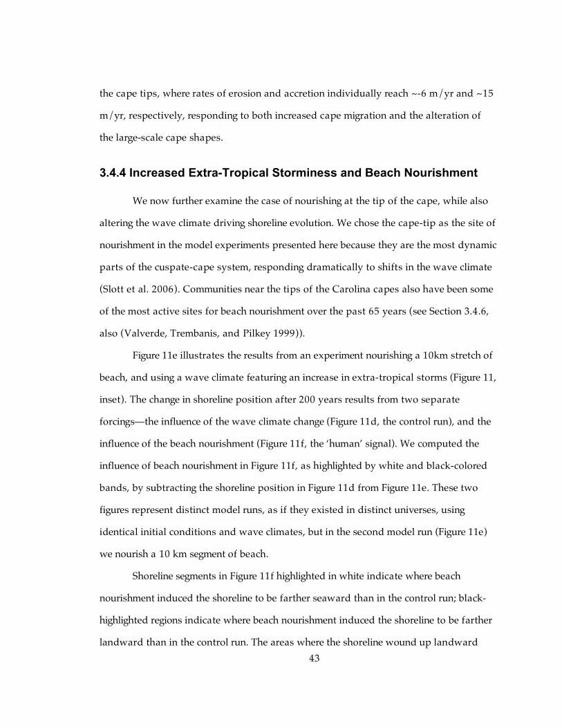
43
the cape tips, where rates of erosion and accretion individually reach ~-6 m/yr and ~15
m/yr, respectively, responding to both increased cape migration and the alteration of
the large-scale cape shapes.
3.4.4 Increased Extra-Tropical Storminess and Beach Nourishment
We now further examine the case of nourishing at the tip of the cape, while also
altering the wave climate driving shoreline evolution. We chose the cape-tip as the site of
nourishment in the model experiments presented here because they are the most dynamic
parts of the cuspate-cape system, responding dramatically to shifts in the wave climate
(Slott et al. 2006). Communities near the tips of the Carolina capes also have been some
of the most active sites for beach nourishment over the past 65 years (see Section 3.4.6,
also (Valverde, Trembanis, and Pilkey 1999)).
Figure 11e illustrates the results from an experiment nourishing a 10km stretch of
beach, and using a wave climate featuring an increase in extra-tropical storms (Figure 11,
inset). The change in shoreline position after 200 years results from two separate
forcings—the influence of the wave climate change (Figure 11d, the control run), and the
influence of the beach nourishment (Figure 11f, the ‘human’ signal). We computed the
influence of beach nourishment in Figure 11f, as highlighted by white and black-colored
bands, by subtracting the shoreline position in Figure 11d from Figure 11e. These two
figures represent distinct model runs, as if they existed in distinct universes, using
identical initial conditions and wave climates, but in the second model run (Figure 11e)
we nourish a 10 km segment of beach.
Shoreline segments in Figure 11f highlighted in white indicate where beach
nourishment induced the shoreline to be farther seaward than in the control run; black-
highlighted regions indicate where beach nourishment induced the shoreline to be farther
landward than in the control run. The areas where the shoreline wound up landward

44
and seaward relative to the control run do not, however, necessarily indicate areas of
overall erosion or accretion over 200 years. Figure 11f, illustrates that white-colored
regions generally coincide with eroding areas in Figure 11d and black-colored regions
generally coincide with areas that accreted in the control run. Localized beach
nourishment tended to counteract the effects of the altered wave climate over a wide
area in this model run. Figure 11f illustrates that the beach nourishment site itself wound
up seaward, relative to the control run, through the net addition of sand. The broad
cuspate bay to the left of the nourishment site also wound up seaward, as did much of
the cuspate bay to the right of the nourishment site. The cape flank downdrift of the
nourishment site wound up as much as 500 m landward relative to the control run after
200 years.
As a measure of the large-scale effects beach nourishment has on shoreline
evolution, we compute the magnitude of shoreline change, expressed as a rate (m/yr):
|r|, the alongshore average of the absolute magnitude of the difference in shoreline
position between the runs with and without beach nourishment, divided by 200 years,
within select distances away from the nourishment site. For the experiment depicted in
Figure 11f, |r| within 10 km of the nourishment site (|r10|), excluding the nourishment
site itself, equals 2.4 m/yr, while |r20| (within 20 km) equals 1.4 m/yr. The magnitude
of these effects approach the rate of shoreline change induced by only changing the wave
climate (~3 m/yr, Figure 11b) (Slott et al. 2006). The effects from beach nourishment
also spread hundreds of kilometers away from the nourishment area. Although the
magnitude of these changes are small compared to the changes tens of kilometers away,
the spatially coherent bands of white and black-colored regions in Figure 11f far away
from nourishment suggests the phenomenon is not random, but a systematic effect of the
beach nourishment. For example, the black-color banded approximately 125 km to the
left of the beach nourishment site in the cuspate bay (Figure 11f) spans 18 km having an
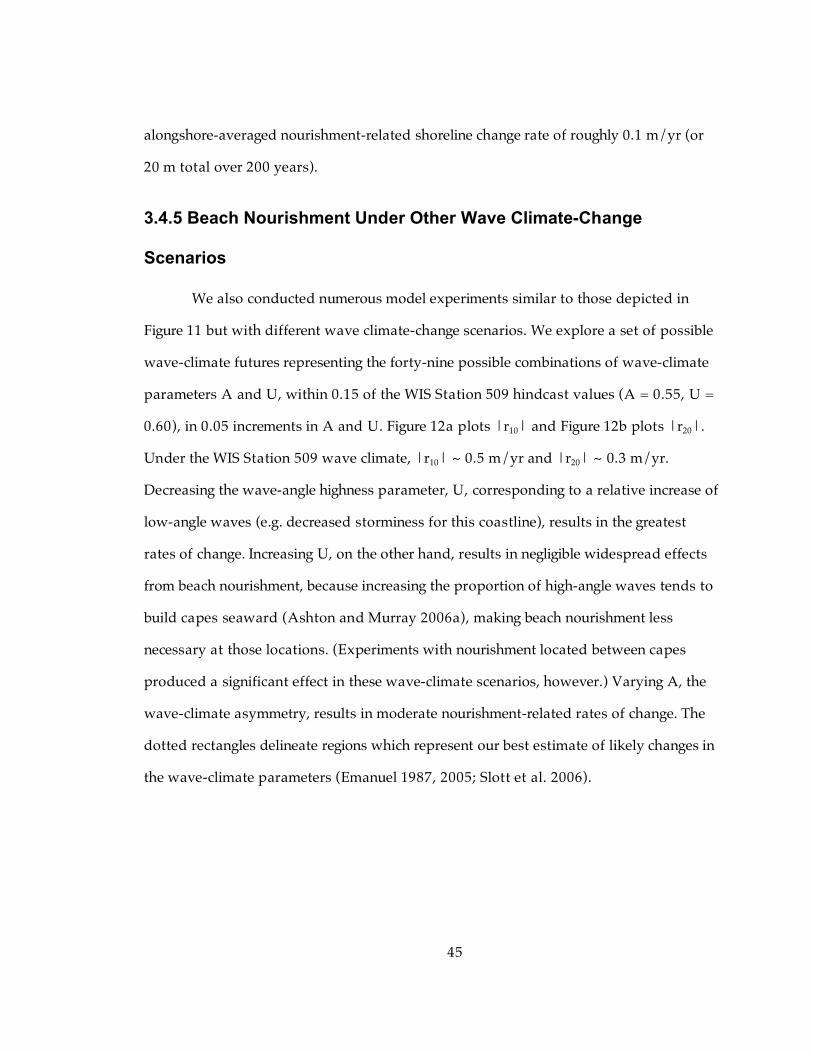
45
alongshore-averaged nourishment-related shoreline change rate of roughly 0.1 m/yr (or
20 m total over 200 years).
3.4.5 Beach Nourishment Under Other Wave Climate-Change
Scenarios
We also conducted numerous model experiments similar to those depicted in
Figure 11 but with different wave climate-change scenarios. We explore a set of possible
wave-climate futures representing the forty-nine possible combinations of wave-climate
parameters A and U, within 0.15 of the WIS Station 509 hindcast values (A = 0.55, U =
0.60), in 0.05 increments in A and U. Figure 12a plots |r10| and Figure 12b plots |r20|.
Under the WIS Station 509 wave climate, |r10| ~ 0.5 m/yr and |r20| ~ 0.3 m/yr.
Decreasing the wave-angle highness parameter, U, corresponding to a relative increase of
low-angle waves (e.g. decreased storminess for this coastline), results in the greatest
rates of change. Increasing U, on the other hand, results in negligible widespread effects
from beach nourishment, because increasing the proportion of high-angle waves tends to
build capes seaward (Ashton and Murray 2006a), making beach nourishment less
necessary at those locations. (Experiments with nourishment located between capes
produced a significant effect in these wave-climate scenarios, however.) Varying A, the
wave-climate asymmetry, results in moderate nourishment-related rates of change. The
dotted rectangles delineate regions which represent our best estimate of likely changes in
the wave-climate parameters (Emanuel 1987, 2005; Slott et al. 2006).

46
Figure 12. Contour plots of nourishment-caused components of shoreline change rates within a, 10 km and b, 20 km of a beach nourishment, excluding the site itself,
for different combinations of wave climate parameters A and U (individual model experiments denoted by ‘+’). Dotted rectangles denote the region where the wave
climate parameters change by at most 0.10 and the center of the plot corresponds to an unchanged wave climate (A = 0.55, U = 0.60).
3.4.6 Beach Nourishment Sand Volumes
Figure 13 shows a contour diagram of the quantity of beach sand (expressed as a
volumetric rate, i.e. cubic meters of sand per kilometer per year) needed to stabilize the
position of the 10 km shoreline region over the course of the 200-year simulation for the
combinations of wave-climate parameters presented in Figure 12. We can make some
initial comparisons from the model run which uses recent wave-climate conditions (A =
0.55, U = 0.60; WIS) to past nourishment practices. Along the North Carolina coastline,
Wrightsville Beach and Carolina Beach have both nourished their beaches at regular
intervals over the past roughly half-century, and continue to do so today (Valverde,
Trembanis, and Pilkey 1999; Beach nourishment histories are catalogued by the Program
for the Study of Developed Shorelines, found at
http://www.nicholas.duke.edu/psds/nourishment.htm, hereafter PSDS), and
furthermore occupy the approximate position relative to their cape tips (i.e. Cape
Lookout, NC) that the beach nourishment site selected for our model experiments in

47
Figure 11 does. Beach nourishment at these two sites represents nearly 40%
(volumetrically) of all beach nourishment activity in North Carolina over the past 65
years (PSDS). Under recent wave-climate conditions the model run placed nearly 18 m3
per meter of shoreline per year. Projects at the two North Carolina locations have
nourished at roughly five to ten times this rate over the past fifty years (~90 m3/m/yr at
Wrightsville Beach and ~163 m3/m/yr at Carolina Beach) (Valverde, Trembanis, and
Pilkey 1999). (Past beach nourishment data for these two locations is, unfortunately
incomplete: in many cases, either the length or sand volume or both are unavailable. For
both locations, however, we simply take the average of the sand volumes and lengths we
do have to compute the volumetric rate of beach nourishment sand placement.) Beach
nourishment project lengths in North Carolina have historically been shorter than our 10
km model length: the fact that longer beach nourishment projects retain their sediment
volume longer may account for some of the discrepancy (Dean 2002). Regardless, this
initial comparison suggests that the model is not unrealistically driving shoreline
evolution by adding too much beach nourishment sand.
Figure 13. Beach nourishment sand volumes for different combinations of wave climate parameters A and U, as in Figure 12 (individual model experiments denote
by ‘+’). Dotted rectangle denotes the region where the wave climate parameters

48
change by at most 0.10 and the center of the plot corresponds to an unchanged wave climate (A = 0.55, U = 0.60).
As a further comparison, the U.S. Army Corps of Engineers planned a 50-year,
recurring beach nourishment project along two segments of coastline in Dare Country,
NC, USA (USACE 2002). After an initial construction phase, the recurring nourishment
volume required to pin the North and South shoreline segments in place over the long-
term more closely resembles model nourishment volumes: 30.5 m3/m/yr is required for
the Northern region (2,167,513 m3 per 23.7 km per 3 years) and 16.0 m3/m/yr is
required for the Southern region (806,605 m3 per 16.8 km per 3 years).
The amount of sand needed to nourish cape-flanking beaches along the Carolina
coast may significantly increase if storm patterns changes, but is highly dependent upon
the exact nature of the change (Figure 13). Cuspate bays will likely require more intensive
shoreline stabilization efforts under wave-climate scenarios that feature proportionally
more high-angle waves. When the intensity of storm activity decreases, the wave climate
is influenced by on-shore winds to a greater degree, and erosion rates at the cape-tips
increase under the more diffusive wave climate. Under these scenarios, the need for
beach nourishment sand to stabilize the position of the cape-tip greatly increases (Figure
13, leftmost side). A shift in the directional asymmetry of the wave climate alone (i.e.
rightward vs. leftward-directed waves) tends to have little effect on beach nourishment
rates.
3.4.7 Interpretation of Physical Mechanisms
As was evident in the experiments involving an initially straight coastline,
adjacent beaches may advance for reasons other than beach nourishment sand
spreading from the nourished area: adjacent areas may advance because the plan-view
perturbation in the beach nourishment area induces a convergence of alongshore

49
sediment transport under asymmetric wave climates (e.g. Figures 8, 9, 11). Beach
nourishment, particularly if it occurs near a cape tip, also alters the extent to which
protruding features shadow adjacent coastlines from incoming waves.
To better understand how these mechanisms influence coastline evolution, we
collected two statistics during each model run: the net alongshore sediment transport
(Qnet) and the influence of wave shadowing on alongshore sediment transport (Qshadow)
for each alongshore position in our model domain. We compute the net alongshore
sediment transport (Qnet) simply as the sum of all fluxes across the right boundary of
each shoreline cell; we count rightward-directed fluxes out of the cell as positive. The
influence of wave shadowing on alongshore sediment transport (Qshadow) is the sum of all
fluxes across the right boundary of each shoreline cell prevented because the cell is
shadowed. (These fluxes would have occurred in a world in which the wave shadowing
mechanism did not exist). If a cell is never shadowed, then its Qshadow is zero.
Figure 14 is a definition sketch that illustrates how we computed the difference in
the fluxes, Q’net and Q’shadow, across the two parallel model runs to analyze the
component of shoreline change induced by beach nourishment. In this sketch we only
consider the flux across a single model cell occupying the same alongshore position in
both runs, and for only one model time-step; we also assume that all fluxes are
rightward-directed for simplicity. In the first two cases (Figures 14a,b) the model cell is
not shadowed; in the first (Figure 14a), the rightward-directed flux (as represented by
solid arrows, where arrow lengths represent relative magnitudes of fluxes) is greater in
the model run without beach nourishment than the model run with beach nourishment. In
the second (Figure 14b), the rightward-directed flux is greater in the model run with
beach nourishment. In the first case, beach nourishment decreases the rightward-directed
sediment flux across the two model runs (a negative flux perturbation, Q’net); in the

50
second case, beach nourishment increases the rightward-directed sediment flux (a
positive flux perturbation, Q’net) across the two model runs.
Figure 14. Definition sketch of model run statistics Q’net, the flux perturbation, and Q’shadow, the extent to which wave shadowing was responsible for Q’net.
Beach nourishment may induce a change in the extent to which a model cell is
shadowed, and is captured by the Q’shadow statistic as is illustrated by the latter two
cases, Figures 14c,d. In the third case (Figure 14c), the model cell is shadowed in the
model run with beach nourishment but not shadowed in the model run without beach
nourishment, and vice versa in the fourth case (Figure 14d). In Figure 14c, the negative
flux perturbation, Q’net, results from an increase in wave shadowing—Qshadow increases

51
from zero (Figure 14c, single dot) in the model run without beach nourishment to a value
in the model run with beach nourishment that accounts for Q’net. (The sum of the flux
values represented by the solid and dotted arrows in the left column equals the sum of
the flux values represented by the arrows in the right column.) Figure 14d shows how a
positive flux perturbation, Q’net, can result from a decrease in wave shadowing—Qshadow
decreases from a positive value to zero (i.e. a negative Q’shadow) and Qnet increases
correspondingly (i.e. a positive Q’net).
Figure 15. Physical mechanisms of human-induced shoreline change. a, A magnification of the shoreline region enclosed in the red dotted rectangle from
Figure 11f. b, A plot of Qnet for the control model run (solid line) and the model run with beach nourishment (dotted line). c, A plot of Qshadow for the control model run
(solid run) and the model run with beach nourishment (dotted line). d, The human-

52
induced perturbation to alongshore sediment flux, Q’net (solid line), where positive (negative) values indicate an excess of rightward-directed (leftward-directed) flux.
The portion of the flux perturbation, Q’shadow, caused by alterations in wave shadowing is also plotted (dotted line). e, Plot of the slope of Q’net.
Figure 15 plots Q’net and Q’shadow for a selected region of shoreline from the model
run shown in Figure 11. Spatial gradients in the flux perturbation correspond to the
relative shift in shoreline position attributed to the beach nourishment activity. A
positive (negative) slope, representing a divergence (convergence) of the flux
perturbation, Q’net, corresponds to areas in which nourishment caused the final position
of the shoreline to wind up further landward (seaward) than it would have otherwise.
Using Figure 15, we can now explain the mechanism through which nourishment
affects shoreline change, beginning with the section of coastline to the left of the
nourishment area that ends up farther seaward because of beach nourishment (denoted
by (1) in Figure 15d). The negative slope of the flux perturbation, Q’net, in this region
indicates that beach nourishment induced a component of the flux convergence. (The
flux convergence induced by beach nourishment is in addition to that induced by the
prevailing wave climate absent any forms of human stabilization.) Sediment from the
nourishment activity does not accumulate in this region because the net alongshore
transport is directed rightward in this area. Rather, by fixing the beach position,
nourishment alters the local shoreline angle the nourishment area makes with its
neighbors, resulting in the flux convergence. Although wave shadowing is affected in
region (1), the change (Q’shadow) does not contribute much to the sediment flux
perturbation, Q’net.
Figure 15 also provides insight into the relative landward shift of the shoreline in
region (2), to the right of the nourishment site. The positive slope of the flux
perturbation, Q’net, shows that beach nourishment induces a component of flux
divergence (Figure 15d, solid line), and furthermore changes to wave shadowing do not

53
play a significant role in the flux perturbation (Figure 15d, dotted line). The flux of
sediment across the left boundary of region (2) decreases while the flux of sediment
across its right boundary only varies slightly. Cape migration is slowed by the shoreline
stabilization, and the sediment that would otherwise have entered region 2 from the left
decreased because of altered shoreline angles.
Wave shadowing does play a key role in spreading the effects from beach
nourishment over greater distances. The magnitudes of the flux perturbations for the
adjacent capes are smaller (Figure 15d, regions 3 & 4, solid line); however wave
shadowing is responsible for nearly all of the flux perturbations (Figure 15d, regions 3 &
4, dotted line).
3.5 Discussion
3.5.1 Sea Level Rise
In our model experiments, we implicitly assume sea level remains constant. We
can expect sea-level rise over the coming century to tend to produce a component of
erosion that will be superimposed on the changes from gradients in alongshore sediment
flux that we address. As a rough approximation, we can estimate the sea-level
component of shoreline change from a geometric conceptual model, where nearshore
sediment mass is conserved while the shoreface and barrier-island profile shifts upward
and landward (Bruun 1962, 1983; Cowell, Roy, and Jones 1995). The rate of shoreline
erosion in such models is sensitive to the geometry assumed for the profile, determined
by the landward and seaward limits of wave-driven sediment transport. In such models,
the component of shoreline retreat rate related to sea-level rise is the sea-level-rise rate
multiplied by the inverse of the average slope of the active profile. The geometry of
active profiles varies spatially, and depends on the timescales involved. Over short

54
timescales, the slope of the upper shoreface, approximately 0.01, is often considered the
relevant part of the profile (Bruun 1962; Zhang, Douglas, and Leatherman 2004). On
timescales longer than the typical return intervals of large storms, the entire composite
barrier island and shoreface profile must be considered, giving a slope that can be
considerably lower. For a specific part of the northern Outer Banks of North Carolina,
this slope is approximately 0.0015 (Laura Moore, pers. comm.). Thus, depending on
time scales and assumptions of geometry, estimates of the component of shoreline
retreat caused by sea-level rise can vary widely, and comparisons between the effects of
human manipulations and sea-level rise can only be order-of-magnitude estimates. Using
the commonly assumed 0.01 slope (Zhang, Douglas, and Leatherman 2004), sea-level
rise may contribute roughly 0.48 m/yr of shoreline erosion, assuming a sea-level rise of
0.48 meters over the coming century (IPCC 2007). (Using the longest-term assumptions
for the profile geometry, the estimated retreat rate would be a few meters per year.) As
demonstrated in Slott et al. (2006), the rate at which the shoreline erodes or accretes
because of moderate changes in storm patterns can reach nearly an order of magnitude
larger than this 0.48 m/yr estimate of sea-level rise erosion rate. The results we present
here suggest that the component of shoreline change induced by nourishment, tens of
kilometers away from a nourishment site, even if prevailing wave climates persist into
the future, are also commensurate with the range of estimates for the sea-level rise
component, and may, under many of the possible wave climate futures (Figure 12) be
greater.
3.5.2 Sensitivity to Model Parameters
In addition to the numerical experiments already presented, we conducted
additional model runs that test the sensitivity of our results to certain input model
parameters. In the model runs presented here, we nourish shoreline segments at every

55
time step (i.e. 1 day), assuming they have eroded beyond their initial position, achieving
the desired modeling goal of pinning the shoreline in place over the long-term. In practice,
beach nourishment typically only takes place every several years, so we test the
sensitivity of our model results to our simplifying model assumption. We repeat our
model runs while varying only the interval at which we conduct beach nourishment. We
test three additional beach nourishment intervals, I (I = 3, 5, and 10 simulated years),
and compare r10 and r20 to the similar statistic from the model run presented in Figure 7e
(Table 1).
Table 1. Sensitivity of model results to beach nourishment interval, I.
I |r10| (± change) |r20| (± change)
1 day 2.4 m/yr 1.4 m/yr
3 yr 2.3 m/yr (-0.1 m/yr) 1.3 m/yr (-0.1 m/yr)
5 yr 2.2 m/yr (-0.2 m/yr) 1.3 m/yr (-0.1 m/yr)
10 yr 2.1 m/yr (-0.3 m/yr) 1.2 m/yr (-0.2 m/yr)
We also tested the model’s sensitivity to our choice of a 10 km beach
nourishment length, since this value exceeds most historical beach nourishment lengths,
instead using lengths of L = 5 km and L = 7 km, while keeping all other model
parameters the same (Table 2). (Although historical lengths have tended to be smaller
than 10 km, recent trends suggest longer beach nourishment projects may become typical
(Valverde, Trembanis, and Pilkey 1999). A single 50-year beach nourishment project
planned for Dare County, NC spans 28 km, for example (USACE 2002).) The increase

56
in these statistics suggests that our large nourishment lengths are not inflating the
magnitude of the results we observe.
Table 2. Sensitivity of model results to beach nourishment length, L.
L |r10| (± change) |r20| (± change)
10 km 2.4 m/yr 1.4 m/yr
7 km 2.6 m/yr (+0.2 m/yr) 1.6 m/yr (+0.2 m/yr)
5 km 2.8 m/yr (+0.4 m/yr) 1.9 m/yr (+0.5 m/yr)
All model run results embody some element of random probability (e.g. random-
number draws from a wave-climate PDF, ref. Section 3.3.3): we conduct duplicate
model runs of previous experiments, yet we use a different random-number generator
seed (resulting, for example, in a different set of incident waves drawn from the same
PDF). We observe that rates of geomorphic change on the coastline vary by ±0.1 m/yr,
on average. The rates of geomorphic change we obtained as a result of many of the
sensitivity tests we conducted above did not significantly exceed this threshold value—
this suggests that the model’s sensitivity to these parameters are indistinguishable from
the stochasticity of wave climate draws. Only when L <= 5 km, did the changes in the
rates of shoreline change significantly exceed the lower-bound threshold value.
3.5.3 Model Simplifications
Our ‘one-contour-line’-based coastline model makes simplifying assumptions,
omitting many smaller-scale sediment transport processes and features specific to the
Carolina coast and cuspate-cape coastlines in general. We ignore any wave diffraction
57
that takes places at the cape tips and the impoundment of alongshore-transported
sediment in extensive shoals extending from the capes (Falqués and Calvete 2005;
McNinch and Leuttich 2000; McNinch and Wells 1999).
We ignore the effects non shore-parallel seabed contours have on wave refraction
(Falqués and Calvete 2005; McNinch 2004). Furthermore, we assume at least a thin
veneer of sediment covers the shoreface at all times; bedrock outcrops on natural
shorefaces can limit the amount of mobile sediment and constrain alongshore sediment
fluxes (Valvo, Murray, and Ashton 2006). This study addresses sandy coastlines; the
response of other types of coastlines (e.g. rocky) to climate change and beach
nourishment may differ (Dickson, Walkden, and Hall 2006). We also assume the
process of sand extraction used for nourishment does not affect the shoreline; we ignore
any effects dredging nourishment sand from ebb tidal shoals has on the
morphodynamics of barrier island systems.
The model treats only instantaneous shifts in wave climates, rather than shifts
which develop gradually over the course of decades. When formulating wave climate
scenarios for possible future changes in warming-induced storminess, we ignore the
effect varying storm activity has on average wave height, representing shifts in the
angular distribution of approaching waves only. (This simplification suggests that we
may be underestimating (overestimating) the effects from increased (decreased) storm
activity on shoreline change, because an increase (decrease) in storminess will also
increase (decrease) average wave heights.) Our future wave climate scenarios are
themselves order-of-magnitude approximations, recognizing the imperfect state of the
science surrounding the link between storm activity and global warming (Donnelly and
Woodruff 2007; Emanuel 2005, 1987; Lambert 1994; Landsea 2005; Pielke, Jr. 2005;
Webster 2005).

58
As such, our model results are not meant to be quantitatively reliable predictions.
Nevertheless these model experiments let us compare the relative influence three primary
drivers—shifts in storminess-related wave climates, direct human modifications to the
shoreline system, and sea-level rise—have on shoreline evolution on time and spatial
scales much greater than are traditionally considered when nourishment effects are
analyzed. When considering the consequences of beach nourishment on shoreline
migration, coastal managers and scientists implicitly assume the effects always result in
adjacent shorelines migrating seaward (Dean 2002). Our work here demonstrates that
this is not always true, particularly when we take into account the large-scale shape and
orientation of the shoreline, the influence of high-angle waves, and the role wave
shadowing plays in transmitting the effects human stabilization has on shoreline
evolution over large-scales within human time-scales. Although sea-level rise garners
much attention from coastal communities, their direct actions to stabilize eroding
beaches may induce effects just as large as the ones they are meant to combat. By
casting direct human manipulations (i.e. beach nourishment) of the shoreline into our
large-scale modeling framework, we can begin to gain an understanding of the complex
and non-local nature of the shoreline response. Future advances in modeling will no
doubt help us understand the nature of these processes in greater detail.
Although we include human actions in our modeling process, we do not explicitly
include the dynamical nature of their decision-making process. In practice, beach
nourishment activity is not static as we have modeled here—the decision to begin
nourishing a beach depends upon a more complex set of conditions beyond the mere
condition that the beach has eroded beyond some ‘initial’ location. Typically,
communities conduct an economic, cost-benefit analysis of proposed beach nourishment;
a favorable outcome to such an analysis is a required to receive federal matching funds
(WRDA 1986). Dynamic capital theory allows us to explore the nature of human,

59
economic decisions in a highly-stylized, single-dimension model of beach nourishment
(Smith et al., manuscript in review). By coupling this model to our spatially-extended
model of the morphodynamic response of coastlines to beach nourishment, we may
observe new, emergent behaviors.
3.6 Conclusion
Despite commonly-held notions, beach nourishment does not always affect
adjacent shoreline segments according to a diffusion-like process: by simply altering the
mix of wave approach angles, we observe a rich set of coastline morphological
responses. On complex-shaped coastlines found in nature (e.g. cuspate-capes), these
varied morphological responses manifest themselves as we select different positions
along the coastline to nourish: local wave climates are governed by the shadowing of
waves in the regional wave climate, as well as by local shoreline-rotation relative to the
regional trend. As we repeatedly nourish towards the tip of a cape, pinning it in place,
the down drift flank tends to move landward in response. Altering the wave climate to
explore the global warming-induced changes we might expect over the coming century,
we find that the human-induced component of shoreline change may be on the same
order of magnitude as sea-level rise.
As a result of humans’ intentional interference with the natural evolution of
coastlines over the past several decades, few coastlines can be considered pristine.
Human interference in the coastal zone will likely intensify in the future. The dramatic,
large-scale effects of locally pinning the coastline in place include a diverse set of
morphological responses with magnitudes comparable to responses to natural processes.
As in many human-natural coupled landscape systems, human manipulations represent
an integral, coastline process: human and natural forces must be considered together
when understanding the morphological evolution of developed coastline systems.

60
4. Synergies Between Adjacent Beach-Nourishing Communities in a Morpho-economic Coupled Coastline Model
4.1 Introduction
This chapter is a preprint of an article in press in Coastal Management Journal,
copyright Taylor & Francis.
Today, many coastal areas experience high rates of shoreline erosion (e.g. a few
meters/year), a trend that is likely to increase over the coming decades as sea-level rise
accelerates and shifting storm patterns rapidly alter coastline configurations (Slott et al.
2006; IPCC 2007; Bruun 1962). Despite this trend, human development along the
coastline also continues to accelerate (Pilkey et al. 1998; Houston 2002), placing more
valuable economic assets in the direct path of coastline erosion. To stave off the loss of
these assets, humans have turned to various shoreline ‘stabilization’ techniques to keep
the position of the shoreline fixed over time. Lately, communities have increasingly
employed beach nourishment, which places additional sand on an eroding beach, over
other techniques, because it, at least temporarily, creates a wide beach for recreational
purposes (Larson and Kraus 1991; Dean 2002). Other stabilization techniques, such as
building seawalls to protect structures, have fallen out of favor; on an eroding shoreline
the sandy beach inevitably disappears in front of a seawall (Pilkey and Wright 1989),
and other methods such as groyne fields that trap sand locally inevitably enhance
erosion elsewhere.
Researchers, when considering the geomorphic consequences of nourishing a
beach, have limited both the spatial and temporal scales of their investigations (Dean
2002). Typically, numerical and occasionally laboratory wave-basin models are
constructed to address questions concerning the ‘life-span’ of a beach nourishment
project (i.e. the rate of loss of nourishment sand) (Dean 2002; Larson and Kraus 1991),

61
or its optimal geometric design (Donahue and Dean 1999; Work and Rogers 1998).
Economic studies of beach nourishment have been designed to compare the costs and
benefits of nourishment to those of other beach management strategies, including
allowing the beach to retreat unabated (Pompe and Reinhart 1994, 1995; Parsons and
Powell 2001; Landry et al. 2003). Like the studies of the physical processes, previous
economic research has typically focused on a single community nourishing only their
beach.
We take a different approach here: we couple a morphodynamic coastline model
to an economic-based, decision-making model, and consider how two adjacent
communities who nourish their respective beaches affect one another. Each community is
assumed to make economically-driven decisions about whether or not to nourish their
beach. Our coupled morpho-economic model of beach nourishment permits the following
feedback: economic-based nourishment decisions affect the geomorphic evolution of the
coastline dynamically, which in turn feeds back into the economic decision-making
model. We conduct model experiments for two communities each with distinct sets of
economic model parameters, and discuss our results in this context. In Section 4.2 we
describe previous numerical coastline and economic models of beach nourishment, and
in Section 4.3 we describe our coupled morphological-economic model and outline the
experiments we run using the model. Section 4.4 presents the model results, while
Section 4.5 explains the significance of our results and offers concluding remarks.
4.2 Background
4.2.1 Numerical Models of Coastline Evolution
Waves breaking at an angle to the shoreline tend to drive a flux of sediment in
both the along-shore and cross-shore directions. Shoreward-directed sediment fluxes,

62
opposed by gravity, shape a cross-shore profile. Although this profile changes on the
time scale of storm cycles, as sand moves offshore during a storm and then back onshore
afterwards (e.g. List and Farris 1999), the long-term average profile shape is typically
treated as constant, and cross-shore sediment losses are assumed to be negligible (Dean
and Maurmeyer 1983; Hanson and Kraus 1989). Under these assumptions, long-term
(i.e. years to centuries) changes in the position of the coastline are governed by gradients
(i.e. alongshore variations) in the wave-driven alongshore sediment flux (Komar and
Inman 1970; Komar 1998, 424-55; Cowell, Roy, and Jones 1995; Ashton and Murray
2006a,b).
Numerical models of the fate of beach nourishment sand typically treat the
cross- and along-shore directions separately (Larson and Kraus 1991). Beach
nourishment sand is placed primarily on the upper portion of the cross-shore profile (the
beach and surf zone), steepening the profile. Gravity and wave action redistribute this
sediment seaward to the lower parts of the profile over the course of months to several
years, tending to return the profile to its equilibrium shape (Dean 2002). Storms may
dramatically accelerate this rate of redistribution, and numerical models (e.g. SBEACH
(Larson, Kraus, and Byrnes 1990)) of cross-shore processes are typically employed to
quantify nourishment sand re-distribution in the presence of storms (USACE 2002).
Another class of numerical models address changes in the plan view (map view)
shape of coastlines, treating changes resulting from gradients in alongshore flux, and
assume cross-shore profile adjustments occur on shorter time-scales (Pelnard-Considere
1956; Hanson and Kraus 1989). In such alongshore-extended models, beach nourishment
is typically represented as a plan-view ‘bump’ in the coastline relative to the local
shoreline trend.
On most coastlines, wave-driven alongshore sediment transport (as a function of
the relative angle approaching wave crests make with the local shoreline orientation,

63
Figure 16a) will tend to smooth out bumps. Recent work (Ashton, Murray, and Arnoult
2001; Murray and Ashton 2003; Ashton and Murray 2006a; Falqués and Calvete 2005)
has shown that, contrary to previous assumptions, when waves approach from deep
water (before nearshore shoaling and refraction) at relative angles greater than
approximately 45o (‘high-angle’ waves), gradients in alongshore transport will cause
large-scale bumps (whether from beach nourishment or occurring naturally) to grow
(Figure 16b). Waves approaching more nearly straight toward shore (‘low-angle’ waves),
on the other hand, tend to cause shoreline undulations to smooth out (Figure 16c) (a
diffusion of plan-view morphology). Over time, waves approach a coastline from a mix
of angles; the proportion of low-angle versus high-angle waves in the ‘wave climate’
determines both whether shoreline ‘bumps’ diffuse or grow and their rate of diffusion or
growth. Regardless of whether the regional wave climate is dominated by high-angle or
low-angle waves, local wave climates for most parts of a shoreline tend to be dominated
by low-angle waves—only those parts which are oriented towards the regional, high-
angle direction of the approaching waves and extend seaward enough to clear other
shoreline protuberances tend to be dominated by high-angle waves from the regional
wave climate (Ashton and Murray 2006b). Therefore, in this work we will treat only
wave climates that smooth the shoreline.

64
Figure 16: After Slott et al. (2006), Schematic illustration of zones of shoreline change caused by the relative wave angle along a curving coastline. a, Alongshore
sediment transport as a function of the relative deep-water angle (before nearshore refraction) approaching waves make with the local shoreline orientation. b, Growth
of a shoreline bump caused by a convergence in alongshore sediment transport when subjected to high-angle waves; and c, smoothing caused by a divergence in
alongshore sediment transport (magnitudes are depicted by varying-length arrows) of a shoreline bump when subjected to low-angle waves.
4.2.2 Economic Models of Beach Nourishment
Most economic modeling of beach nourishment compares the monetary benefits
from beach nourishment to its costs—a favorable outcome of such an analysis is
required before federal funding of a project is made available (Water Resources
Development Act of 1986). The U.S Army Corps of Engineers GRANDUC (Generalized
Risk and Uncertainty – Coastal) (USACE 2002) model, for example, computes the
damage to property (including that of home contents and land loss) if beach
nourishment did not take place and compares that amount to the cost of beach
nourishment. It introduces the effects storms have on beach and property loss by using

65
the SBEACH (Larson, Kraus, and Byrnes 1990) numerical model driven by historical
storm patterns for the region. In these economic models, the time interval between
successive beach re-nourishments is fixed and determined by the expected longevity of
the sand on the beach, absent any major storms (Dean 2002; USACE 2002). Extensive
surveys of individual property values, beach widths, and elevation profiles for the site
feed into the model. Dean (1988) recognized that nourishment sand spread to adjacent
beaches by alongshore sediment transport increases the total benefits for the entire
area—the increase in recreational and storm protection benefits to initially narrow
adjacent beaches more than offsets the loss in benefits from the wider nourished beach.
Some economic studies, using hedonic analysis, have estimated the value a unit-
width of beach has on property values, finding that property values increase as beach
width increases, but with diminishing returns (Pompe and Rinehart 1994, 1995). Other
studies estimate various benefits and costs of methods to preserve a beach and protect
the property and infrastructure behind it, including: 1) the expected reduction of damage
to property from storms afforded by wider beaches (Pompe and Rinehart 1995) and
shoreline armoring (Kriesel et al. 1993); 2) the cost of removing homes as beaches erode
(Landry et al. 2003; Parsons and Powell 2001); and 3) the economically optimal choice
between several beach preservations policies (Landry et al. 2003). Studies that quantify
various beach protection policies (Landry et al. 2003; Parsons and Powell 2001) assume
the shoreline and any sand placed on the beach through nourishment retreats uniformly
over space and time, and that the stabilization policy remains unchanged through time
(i.e., under a beach nourishment management policy, the time-interval at which
nourishment occurs remains fixed).
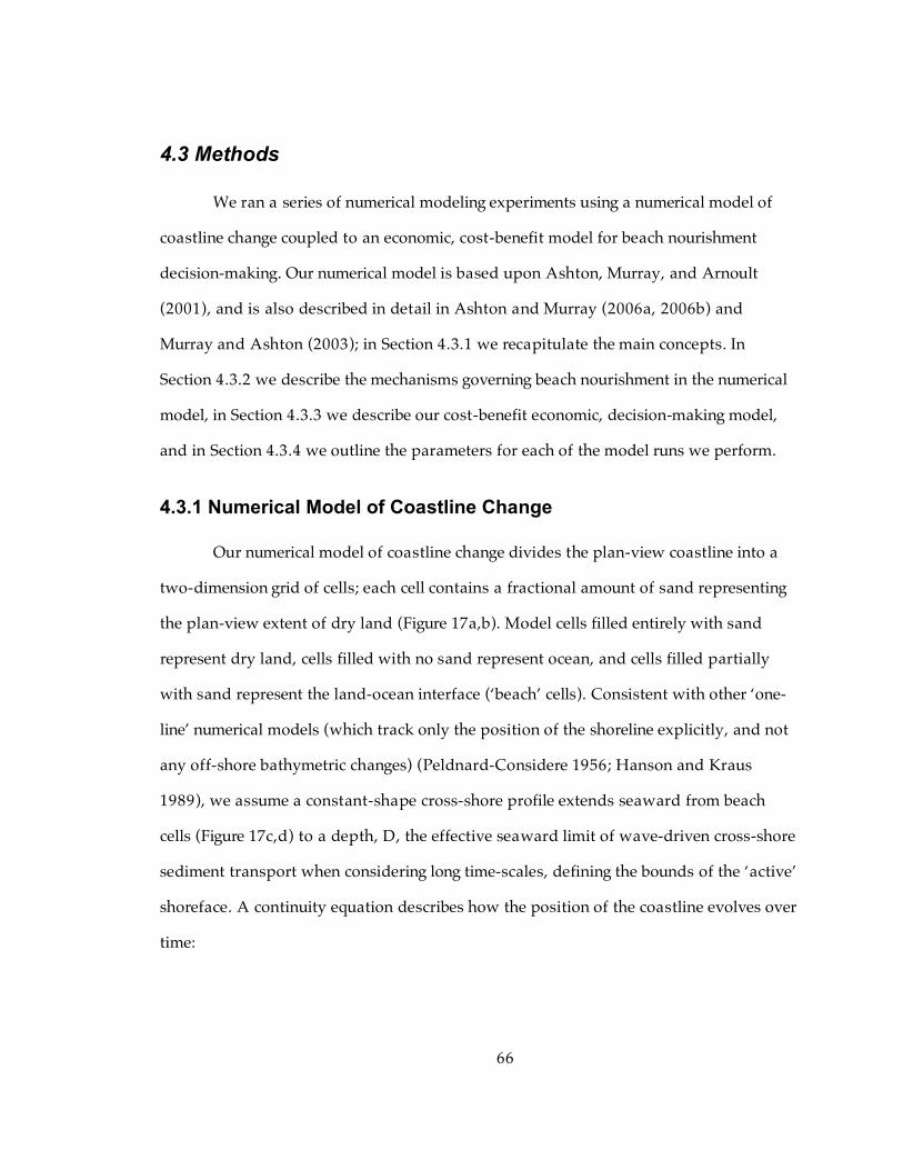
66
4.3 Methods
We ran a series of numerical modeling experiments using a numerical model of
coastline change coupled to an economic, cost-benefit model for beach nourishment
decision-making. Our numerical model is based upon Ashton, Murray, and Arnoult
(2001), and is also described in detail in Ashton and Murray (2006a, 2006b) and
Murray and Ashton (2003); in Section 4.3.1 we recapitulate the main concepts. In
Section 4.3.2 we describe the mechanisms governing beach nourishment in the numerical
model, in Section 4.3.3 we describe our cost-benefit economic, decision-making model,
and in Section 4.3.4 we outline the parameters for each of the model runs we perform.
4.3.1 Numerical Model of Coastline Change
Our numerical model of coastline change divides the plan-view coastline into a
two-dimension grid of cells; each cell contains a fractional amount of sand representing
the plan-view extent of dry land (Figure 17a,b). Model cells filled entirely with sand
represent dry land, cells filled with no sand represent ocean, and cells filled partially
with sand represent the land-ocean interface (‘beach’ cells). Consistent with other ‘one-
line’ numerical models (which track only the position of the shoreline explicitly, and not
any off-shore bathymetric changes) (Peldnard-Considere 1956; Hanson and Kraus
1989), we assume a constant-shape cross-shore profile extends seaward from beach
cells (Figure 17c,d) to a depth, D, the effective seaward limit of wave-driven cross-shore
sediment transport when considering long time-scales, defining the bounds of the ‘active’
shoreface. A continuity equation describes how the position of the coastline evolves over
time:

67
x
Q
Dt
tx s
!
!"=
!
! 1),(# (9)
where η is the cross-shore shoreline position, x is the along-shore coordinate, Qs
is the along-shore sediment transport flux, and D is the aforementioned depth-limit.
Equation 9 has the following interpretation in our model: changes in the cross-shore
position of each beach cell after each model time-step vary with the net sediment
transport into and out of the beach cell (the difference between the sediment past the
left-most and right-most cell boundary). Any sediment that accumulates in a beach cell
spreads seaward evenly to depth, D, shifting the entire active shoreface profile seaward;
similarly, erosion within a beach cell shifts the entire active shoreface profile landward.
Figure 17: ‘One-Line’ modeling approach. Gradients in along-shore sediment transport (Qs) cause: a, Accretion, a convergence in along-shore sediment transport flux, when wave-driven currents transport more sediment into the model cell than
out of the model cell; b, Erosion, a divergence in along-shore sediment transport flux, when wave-driven currents transport more sediment out of the model cell than
into the model cell. c, During accretion, the entire cross-shore profile, represented here and in Ashton, Murray, and Arnoult (2001) as linear, shifts seaward; d, During
erosion, the entire cross-shore profile shifts landward.

68
Our model computes alongshore sediment transport, Qs, using a variant of the
commonly-used CERC (Coastal Engineering Research Center) formula:
!
Qs = KHb
5 / 2sin("b #$)cos("b #$) , (10)
where Hb is the wave height at breaking, φb is the wave angle at breaking, θ is the
local shoreline angle, and K is an empirical constant equal to 6.4 x 10⁴ m3d-1. (Komar and
Inman 1970; Komar 1971; Komar 1998, 390-3; Ashton, Murray, and Arnoult 2001). The
value of K depends upon a host of location-specific geologic factors, and should ideally
be calibrated for each site (Komar and Inman 1970). Since our work does not treat one
specific locale, we choose a value for K representing a fit to previous field experiments
along the US Atlantic coastline (Slott et al. 2006). Model waves approaching from deep-
water refract and shoal over shore-parallel contours as they enter shallower water; the
resulting breaking-wave height and angle are then used in Equation 10.
We represent the distribution of angles from which deep-water waves approach
the shoreline with a cumulative distribution function (CDF) of deep-water wave
approach angles (the ‘wave climate’); each wave is given a deep-water wave height of
1.7m, an effective average wave height (for sediment transport purposes) for a location
off of the US Southeast Coast used in previous work (Slott et al. 2006; Ashton and
Murray 2006a, 2006b). Two parameters, A and U, describe the wave climate CDF. The
wave-angle asymmetry parameter, A, gives the cumulative probability of a wave
approaching from the left, looking off-shore. The wave-angle obliquity parameter, U,
gives the cumulative probability a wave approaches from high-angles (i.e. greater than
45o, the approximate angle which maximizes along-shore sediment transport).
Representing the wave climate using these two parameters makes clear the relationship

69
between coastline behavior and the angular distribution of approaching waves: wave
climates featuring values of A greater than (less than) 0.50 result in net along-shore
sediment transport to the right (left), looking off-shore; and wave climates featuring
values of U greater than (less than) 0.50 result in the growth (anti-diffusion) of shoreline
‘bumps’. For each model run, we choose A and U to represent the wave climate of
interest.
At the beginning of each (simulated) day, our model randomly generates a new
wave from the wave climate distribution as follows. We perform two random-number
draws (r1 and r2) between 0 and 1, one for each of the wave climate CDF parameters A
and U. If r1 < A, the wave approaches from the left, otherwise if r1 >= A, the wave
approaches from the right. If r2 < U, the model randomly (from a uniform distribution)
selects a wave approach angle between 0° and 45° (inclusive), otherwise if r2 >= U the
model randomly selects a wave approach angle between 45° (exclusive) and 90°.
4.3.2 Beach Nourishment
We designate selected stretches of shoreline as communities, and whenever the
shoreline position for these locations falls behind its initial position, the community may
elect to nourish its beach. The model nourishes segments of coastline by adding sand to
beach cells to bring the shoreline back to its original position. On natural beaches,
nourishment disturbs the cross-shore equilibrium profile shape since sand is typically
placed only in the surf/swash zone; the profile is typically restored, however, over the
coming months to years by wave action (Dean 2002). We do not explicitly include this
transient state in the model, because we are addressing coastline behavior on larger time-
scales (years to decades). We also do not consider the short-term effects storms have on
redistributing beach nourishment sediment over the cross-shore profile, unlike numerical
models such as SBEACH (Larson, Kraus, and Byrnes 1990). Instead, the model assumes

70
sand from beach nourishment spreads evenly over the active shoreface profile from the
outset (Figure 17c,d). Since the total cost of beach nourishment depends, in part, upon
the volume of sand placed on the beach, we compute the volume by multiplying the
cross-shore width added to the beach, the along-shore length of the project (e.g. 10 km),
and the seaward depth limit of the active shoreface (Figure 17c,d, 10 m).
4.3.3 Cost-Benefit Economic Model
A community in the model nourishes it beach only when the economic benefits
outweigh the total costs of the beach nourishment activity. On actual shorelines, the
economic benefits of beach nourishment, from an increase in the width of the beach,
include increased property values, increased protection from storm damage for homes
and infrastructure, and increased recreational value (Pompe and Reinhart 1994, 1995;
Landry et al. 2003, Parsons and Powell 2001). Here we consider only the impact wider
beaches have on property values. We model the economic benefit to property values, B,
as a function of beach width:
!
B(w) ="w# (11)
where w is the width of the beach, and α and β are constants. The value of a
property is a function of its characteristics (e.g. the number of bedrooms) and
environment (e.g. the quality of its neighborhood); previous hedonic studies assign
coefficients to constituent parameters representing the property value. We, however,
gather the influence of all characteristics other than beach width on property value into a
single parameter, α, which we interpret as the ‘base property value’. As beach width
increases, property values increase, but to a decreasing extent. Most studies do not
estimate a value of beach width. Studies that do, find in constant elasticity form,

71
β = 0.2632 (Pompe and Rinehart 1995) using only beachfront properties in the sample and
β = 0.085 (Landry 2007) using all barrier island properties in their hedonic property model. We
use 0.2 in our numerical simulations that model nourishment as if there is just a single
row of houses. For future work that is empirically tied to whole beach communities, the
approach in Landry (2007) is likely more appropriate.
We model the cost of beach nourishment as the sum of fixed and variable costs.
Fixed costs, which do not depend upon the amount of nourishment sand dredged,
include activities such as surveys to identify suitable nourishment sediment,
environmental impact studies, permitting, and dredge mobilization. Variable costs
depend upon the volume of nourishment sand dredged and placed on the beach.
Translating between the cross-shore width that nourishment extends the beach and total
volume assuming a linear profile as in Section 4.3.1, the total cost of a single beach
nourishment episode is:
!
C(wn ) = f + cwnLD (12)
where f represents fixed costs, c is the unit-volume cost of beach nourishment
sand, wn is the cross-shore nourishment width, L is the along-shore extent of the beach
nourishment (10 km), and D is depth-limit of wave action (10 m). In our baseline model
experiments, we assign a fixed cost, f, of $1 million and a unit-volume cost, c, of $5/m3
and then vary these parameter values to conduct sensitivity analysis. These baseline
values represent approximations to real-world values--for example, fixed costs for
planned nourishment projects located in Dare County, North Carolina, USA average
~$1.26 million (for mobilization, demobilization, and preparatory work) and unit-
volume costs average ~$4.6/ m3 (for pipeline dredging and beach fill), excluding costs
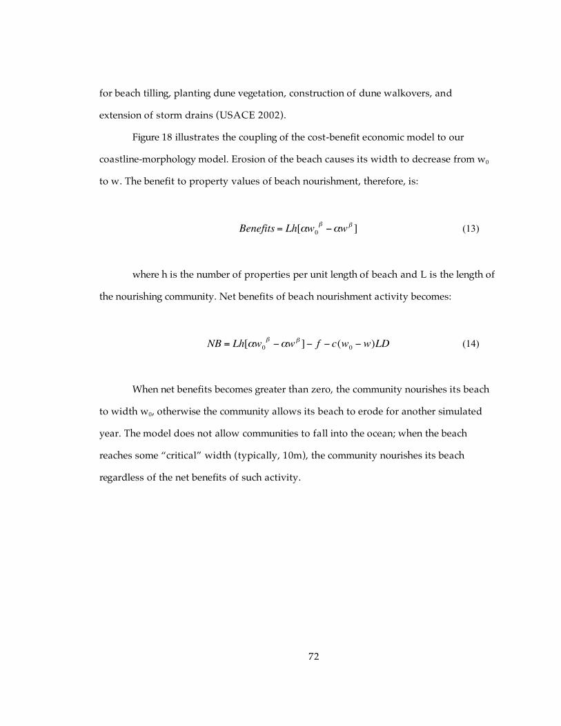
72
for beach tilling, planting dune vegetation, construction of dune walkovers, and
extension of storm drains (USACE 2002).
Figure 18 illustrates the coupling of the cost-benefit economic model to our
coastline-morphology model. Erosion of the beach causes its width to decrease from w0
to w. The benefit to property values of beach nourishment, therefore, is:
!
Benefits = Lh["w0
#$"w#
] (13)
where h is the number of properties per unit length of beach and L is the length of
the nourishing community. Net benefits of beach nourishment activity becomes:
!
NB = Lh["w0
#$"w#
]$ f $ c(w0$ w)LD (14)
When net benefits becomes greater than zero, the community nourishes its beach
to width w0, otherwise the community allows its beach to erode for another simulated
year. The model does not allow communities to fall into the ocean; when the beach
reaches some “critical” width (typically, 10m), the community nourishes its beach
regardless of the net benefits of such activity.

73
Figure 18: Coupling a numerical and economic model of beach nourishment in plan view. A community (dark band) of alongshore length, L, consisting of h properties per kilometer and initial beach width, w0, nourishes its beach when a cost-benefit analysis is favorable,
perhaps when its beach width falls to w. The entire coastline retreats uniformly at a rate r m/yr.
4.3.4 Model Experiments
In our primary set of model experiments, we conduct a series of three individual,
200-year model runs (Figure 19), where we co-locate two nourishing communities on an
initially straight coastline subjected to a uniform erosion rate of 1 m/yr. The two
communities differ in their base property value (‘α’) and the initial width of the beach
(‘w0’). We designate the first community as “poor” (α = $200,000, w0= 100 m) and the
second community as “rich” (α = $400,000, w0= 200 m). We refer to “poor” and “rich”
communities only as relative terms—we do not intend to model specific demographics or
the complex nature of socio-economic interactions between rich and poor communities.
Rather, we are simply considering scenarios where we co-locate two beach communities
that, according to a cost-benefit analysis, can nourish their beach to different degrees. In
our model experiments, the “rich” community, because its higher base property value
offsets beach nourishment’s fixed costs sooner, can nourish its beach more frequently.
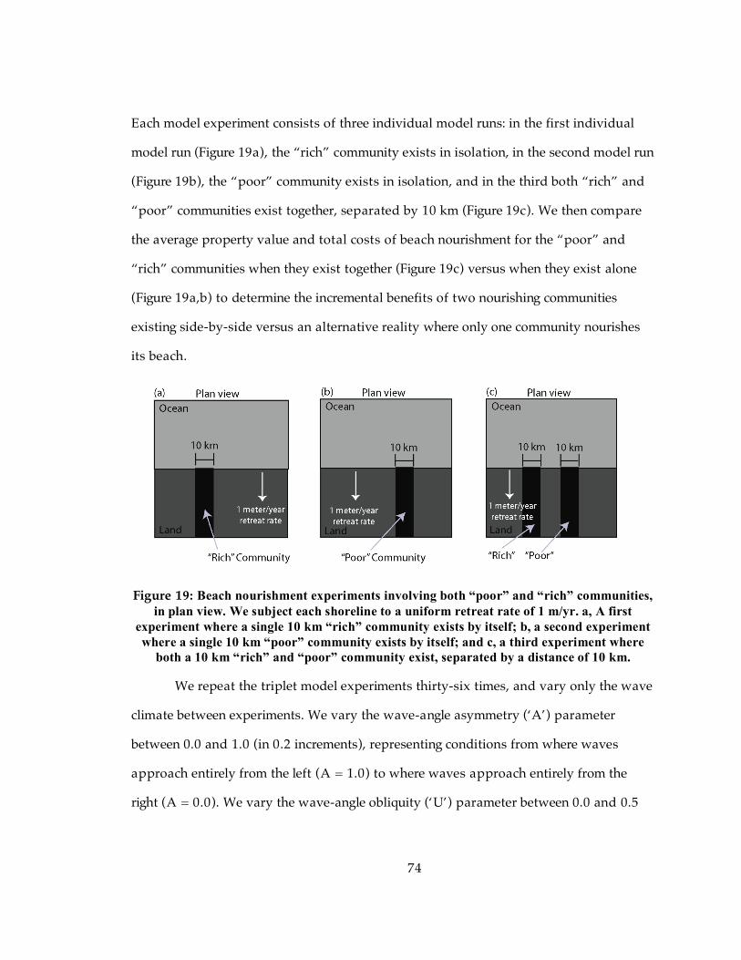
74
Each model experiment consists of three individual model runs: in the first individual
model run (Figure 19a), the “rich” community exists in isolation, in the second model run
(Figure 19b), the “poor” community exists in isolation, and in the third both “rich” and
“poor” communities exist together, separated by 10 km (Figure 19c). We then compare
the average property value and total costs of beach nourishment for the “poor” and
“rich” communities when they exist together (Figure 19c) versus when they exist alone
(Figure 19a,b) to determine the incremental benefits of two nourishing communities
existing side-by-side versus an alternative reality where only one community nourishes
its beach.
Figure 19: Beach nourishment experiments involving both “poor” and “rich” communities, in plan view. We subject each shoreline to a uniform retreat rate of 1 m/yr. a, A first
experiment where a single 10 km “rich” community exists by itself; b, a second experiment where a single 10 km “poor” community exists by itself; and c, a third experiment where
both a 10 km “rich” and “poor” community exist, separated by a distance of 10 km.
We repeat the triplet model experiments thirty-six times, and vary only the wave
climate between experiments. We vary the wave-angle asymmetry (‘A’) parameter
between 0.0 and 1.0 (in 0.2 increments), representing conditions from where waves
approach entirely from the left (A = 1.0) to where waves approach entirely from the
right (A = 0.0). We vary the wave-angle obliquity (‘U’) parameter between 0.0 and 0.5

75
(in 0.1 increments), representing conditions from where the wave climate is neutrally-
diffusive (U = 0.5) to where the wave climate is strongly-diffusive (U = 0.0).
Subsequent model runs test the sensitivity of the results (i.e. average property
value, total nourishment costs) as we vary two other model parameters—the distance
separating each community (5 – 50 km) and beach nourishment cost increases (0 –
100%).
4.4 Results
4.4.1 Varying Wave Climates
As the shoreline retreats during our 200-year model runs, we naturally expect the
nourished segments of shoreline to remain roughly at their initial cross-shore position,
while most other parts of the shoreline should erode 0.2 km after 200 years of 1 m/yr
erosion. (Since communities only nourish after favorable cost-benefit analyses, they may
erode behind their initial positions during the inter-nourishment years). Adjacent
segments of shoreline also benefit from a community’s beach nourishment, winding up
significantly seaward of the 0.2 km loss, evident from the plan-view plots of shoreline
position for two selected model runs, one with a single nourishing community (Figure
20a) and another with two nourishing communities (Figure 20b). Both of these model
runs feature a wave climate where waves approach entirely from the left (A = 1.0) and
entirely from low-angles (U = 0.0). Alongshore sediment transport is always directed
rightward, and smooths any plan-view perturbations to the shoreline, resulting in the
accretion in adjacent areas.

76
Figure 20: Shoreline position for one and two nourishing communities over 200 years, in plan view. In each, a highly-asymmetric (A = 1.0) and highly-diffusive (U = 0.0) wave climate was used, resulting in rightward-directed alongshore sediment transport. a, A
vertical scale-exaggerated plot of shoreline position when only the “rich” community exists. Adjacent sections of coastline on both sides benefit. b, A vertical scale-exaggerated plot of
the shoreline position when both the “rich” and “poor” community exist. Adjacent sections of coastline on both sides benefit; the section of coastline between the two communities
greatly benefits. c, A schematic illustration of why adjacent coastline segments benefit from beach nourishment. Updrift (to the left) of the beach nourishment project, an increase in shoreline angle decreases alongshore sediment transport (AST) leaving that area (dashed
rectangle), resulting in a convergence of AST and accretion of the shoreline. Magnitudes of AST are represented by varying-length arrows following the local shoreline contour.
Downdrift (to the right) of the beach nourishment project, an increase in shoreline angle increases AST entering the area, resulting in a convergence of AST and accretion of the
shoreline there too. d, A schematic illustrations of why both adjacent coastline segments and the coastline segment between the two communities benefits.
The model results presented in Figure 20 show how shorelines on either side of
the beach nourishment project (i.e. both ‘updrift’ and ‘downdrift’) accrete symmetrically
despite the prevailing rightward direction of alongshore sediment transport. Accretion in

77
the downdrift direction from beach nourishment results from the lateral diffusion of
nourishment sediment—the angle the local shoreline makes with the approaching wave
decreases as we move past the rightmost boundary of the nourishment area, and
alongshore sediment transport decreases (ref. Figure 16a for relative angles < 45o). The
result is a convergence of alongshore sediment transport and shoreline accretion in the
downdrift area adjacent to the nourishment project. (The relative angle the shoreline
makes with the approaching waves can be seen in Figure 20c,d by comparing the angle of
the wave crests with the angle of the arrows following the shoreline contour.) Adjacent
areas updrift of the beach nourishment project experience accretion and a convergence in
alongshore sediment transport too—the angle the local shoreline makes with the
approaching wave also decreases as we move toward the project area. (Wherever the
shoreline curvature is concave-seaward, low-angle waves will cause the shoreline to
accrete.) The updrift area accretes, therefore, not because of the lateral diffusion of
beach nourishment sediment, but rather because beach nourishment alters the local
shoreline angles. This phenomenon makes it appear as if beach nourishment sediment
spreads in the opposite direction of alongshore sediment transport; instead, rightward-
migrating sand is ‘trapped’ by the re-orientation of the local shoreline caused by the
beach nourishment project.
After each 200-year model experiment, we computed the average property value
and the total cost of beach nourishment activities. We plotted the total cost of beach
nourishment in Figure 21 for all thirty-six combinations of wave climate parameters for
the “poor” community when it exists alone (Figure 21a), for the “rich” community when
it exists alone (Figure 21b), and for the “poor” and “rich” communities when they exist
together (Figures 21d and 21e, respectively). Figure 21c sums the values in Figure 21a
and Figure 21b; Figure 21f sums the values in Figure 21d and Figure 21e. Note that we do
not discount the nourishment costs, so our model implicitly assumes that property

78
values and nourishment costs grow at the nominal discount rate. The average property
value for the “poor” and “rich” communities was roughly constant ($0.488 million and
$1.144 million, respectively), varying at most by 1% over all experiments.
Figure 21: Contour plot of total undiscounted costs of beach nourishment experiments from Figure 19, for thirty-six combinations of wave climate parameters, A and U. Wave climates range from highly-diffusive (U = 0.0) to neutrally-diffusive (U = 0.5) and range from waves approaching entirely from the right (A = 0.0) to waves approaching entirely from the left (A
= 1.0). a, Total nourishment costs for a “poor” community when it exists alone; b, total nourishment costs for a “rich” community when it exists alone; c, the sum of nourishment
costs from a, and b,; d, total nourishment costs for a “poor” community when it exists adjacent to a “rich” community; e, total nourishment costs for a “rich” community when it
exists adjacent to a “poor” community; f, the sum of nourishment costs from d, and e,.
When performing nourishment in isolation, the “rich” community nourished every
~5.0 years and the “poor” community nourished every ~8.6 years, averaged over the
entire model experiment. When the two communities exist together, nourishment
frequencies decreased: the “rich” community nourished every ~5.5 years and the “poor”
community nourished every ~9.8 years, averaged over the entire model experiment.

79
Nourishment frequencies increased as the wave-climate diffusivity (a measure of the
strength of the coastline-smoothing effect) increased, from ~8.7 years under neutrally-
diffusive wave climates (U = 0.5) to ~6.1 years under entirely-diffusive wave climates
(U = 0.0), averaged over all model experiments.
The “rich” community spent moderately more money on beach nourishment,
because its higher base property values afforded a more frequent favorable cost-benefit
outcome by overcoming the fixed costs sooner. Nourishment costs are sensitive to wave-
angle obliquity--costs double from neutrally-diffusive wave climates (U = 0.5) to highly
diffusive wave climates (U = 0.0). Nourishment costs are not sensitive to wave-angle
asymmetry (A), however.
Also, when the “poor” and “rich” communities exist together (as compared to
when they exist alone) they both spend less money on beach nourishment individually
(Figure 21a,b vs. Figure 21d,e) and in total (Figure 21c vs. Figure 21f), to achieve the
same average property value, suggesting that a synergy exists between two adjacent
nourishing communities. These synergist effects are most pronounced for highly-diffusive
wave climates. Under highly-diffusive wave climates (e.g. U = 0.0 – 0.1), the two
communities saved approximately 25% in nourishment costs when they exist side-by-
side versus when they existed alone. By existing together, the two nourishing
communities help mitigate the cost-doubling under highly-diffusive wave climates as
noted above.
When two communities nourish in tandem, their respective beaches retreat
landward more slowly than if they were alone. This is not necessarily because one
community’s sand spreads onto the beach of the second community, however. The
nature of alongshore diffusion suggests that the erosion in the central (perhaps
‘undeveloped’) area between the communities is mitigated either from sand from a
community’s ‘inner’ edge spreading towards the center, or by sand trapped by the beach

80
nourishment project (Figure 20d). The shoreline angle each community makes with this
central, undeveloped section decreases, as compared to the case of only one nourishing
community. As the shoreline angle decreases, so does alongshore sediment transport
(under a dominantly low-angle wave regime), which, in turn, slows the rate of diffusion
of the plan-view, beach nourishment shoreline perturbation. It is this mechanism by
which communities separated by distances of many tens of kilometers experience the
synergistic effects shown in Figure 21; shoreline-reorientation effects from beach
nourishment spread along the shoreline more quickly and to a greater overall distance
than the nourishment sand migrates itself.
The central, ‘undeveloped’ segment of coastline also inadvertently and greatly
benefits from beach nourishment—if no nourishment at all takes place, this stretch of
coastline would retreat 200 m (1 m/yr over 200 years), but instead only retreats (on
average) approximately 78 m (with only the “poor” community), 74 m (with only the
“rich” community), and 17 m (with two nourishment communities), over 200 years
under a highly-diffusive, symmetric wave climate (A = 0.5, U = 0.0).
4.4.2. Varying Distance Separating Communities
Figure 22 plots the total beach nourishment costs for the “rich” and “poor”
communities when they exist together under a symmetric, highly-diffusive wave climate
(A = 0.5, U = 0.0) and varying the distance separating the two. We compute the total
beach nourishment costs over the 200 year model run using a modified form of Equation
12: we multiply the fixed costs for a single nourishment episode by the total number of
episodes and sum the individual beach widths from each nourishment episode to
determine the variable costs. The two horizontal dashed lines in Figure 22 represent the
total nourishment costs when the two communities exist alone, $61.23 million for the
“poor” community and $63.64 million for the “rich” community. When the communities

81
are separated by 5 km, the total nourishment costs fall to $41.70 million for the “poor”
community (a decrease of ~32%) and $46.66 million for the “rich” community (a
decrease of ~27%). The two communities may see synergistic effects even if they are
separated by as much as 30 km (~4% reduction in costs), but the cost reductions fall to
< 1% beyond that.
Figure 22: Total undiscounted costs of beach nourishment for “poor” and “rich” communities when they exist together and separated by varying distances, ranging from 5
km to 50 km. The two horizontal dotted lines represent total costs of beach nourishment for each community in separate experiments when they exist alone, for comparison.
4.4.3 Increased Nourishment Costs
We also explored scenarios involving different levels of public (in particular,
federal) funding of beach nourishment activities. The Water Resources Development Act
of 1986 established the federal share of beach nourishment costs at 65% (provided the
project meets several requirements, one of which is a favorable cost-benefit analysis)
(Water Resources Development Act of 1986). The federal share of nourishment costs
declined to 50% with the act’s renewal in 1999 (Water Resources Development Act of
1999), and a further reduction to 35% has been proposed (U.S. House 2002, H 6473). In

82
these experiments, we assume any reduction of federal spending on beach nourishment
would impact only the “poor” community (assuming the “rich” community does not
accept federal matching funds today). Even though a loss of federal matching would
likely increase costs for both communities, we vary only the costs to the “poor”
community by some percentage increase, reflecting its increased dependency upon
federal support for beach nourishment and as an experimental simplification.
Figure 23 shows the results of one such experiment using a highly-diffusive wave
climate (A = 0.50, U = 0.0). Both the “poor” community (Figure 23a) and “rich”
community (Figure 23b) exist together, separated by 10 km. Like previous experiments,
we computed and plotted the total nourishment costs (Figure 23, solid line) and the
average property value (Figure 23, dashed line) over the 200-year simulation, for varying
levels of cost increases for the “poor” community, ranging between 0% and 100%. As the
costs to the “poor” community increases from 0% to 100%, its beach nourishment costs
decrease from $46.79 million to $24.80 million (i.e. by roughly 47%), reflecting its
diminished ability to nourish its beach through less frequent favorable cost-benefit
outcomes. Its average property value also falls from ~$0.488 million to ~$0.430 million,
a decrease of ~12%. The “rich” community is also affected by the decrease in
nourishment activity of the “poor” community: as the costs to the “poor” community
increases from 0% to 100%, the “rich” community’s beach nourishment costs increase
from $50.40 million to $58.62 million (i.e. by roughly 16%) while its average property
value remains virtually the same.

83
Figure 23: Total undiscounted costs of beach nourishment (solid line) and average property value (dotted line) for “poor” and “rich” communities when they exist together, as the
federal share of nourishment costs decreases. Cost share borne by the “rich” community is fixed so that federal share reductions affect the “poor” community relative to the “rich”
community. Cost increases for the “poor” community range from 0% (same cost for “poor” and “rich”) to 100% (costs double for “poor” versus “rich”).
4.5 Discussion and Conclusion
Our experiments with a coupled morpho-economic model of beach nourishment
show how two adjacent communities, when nourishing their beaches in tandem,
mutually benefit one another by stabilizing the angle each community makes with its
adjacent shoreline and reducing the effects of alongshore diffusion of sediment.
Surrounded by two nourishing communities, the central ‘undeveloped’ segment of
coastline benefits dramatically without spending any money on beach nourishment. The
fact that the effects were uniform over the entire range of wave-angle asymmetries
suggests that the diffusive nature of the wave climate was far more important than the
net direction of alongshore sediment transport. In terms of our two communities, the
“rich” community does not unfairly benefit if it happens to be “downdrift” of a “poor”
community (and visa versa)—in fact, any notion of “updrift” or “downdrift” in the
context of a diffusive wave climate seems meaningless. Two adjacent nourishing

84
communities approximate a single, long beach nourishment project to some degree; it is
commonly believed that longer beach nourishment projects “perform” better (i.e. last
longer) than shorter projects (Dean 2002).
Total cost of beach nourishment was highly sensitive to the rate of alongshore
diffusion however, and increases in costs under highly-diffusive wave climates was
partially offset by the synergistic effects of two adjacent nourishing communities. This
suggests that in order for models to correctly predict the short-term performance of
beach nourishment projects, estimates of wave climates are needed. However, small
fluctuations about a long-term wave climate can appreciably affect shoreline diffusivity
(Valvo, Murray, and Ashton, 2006), which will decrease the efficacy of short-term
performance predictions.
In the case where the “poor” community’s ability to nourish decreases (perhaps
as a result of a reduction in federal funding), the adverse effects are mitigated to a
degree by the ability of the “rich” community to continue its beach nourishment activities
unimpeded. The “rich” community, whose higher base property values allow it to absorb
the decreased benefits it receives from the “poor” community, increases its investment in
beach nourishment to maintain its average property values at previous levels, while
allowing the “poor” community to become somewhat of a free rider.
Our numerical model of coastline change includes a number of simplifications of
coastal processes. For example, we choose a single, average value for the empirical
coefficient, K, in Equation 10—this parameter is typically calibrated for each site
(Komar and Inman 1970). Also, we assume the shoreline is perfectly straight and ignore
gradients in alongshore sediment transport that may result from subtle, existing
undulations in the shoreline (Ashton, Murray, and Arnoult 2003; Lazarus and Murray
2007). We also assume the shoreline erodes at a uniform rate for the entire beach—highly
variable and heterogeneous rates of shoreline migration locally, however, may result from

85
wholesale shifts in shoreline position occurring on large-scales (Slott et al. 2006) or from
accelerated rates of sea-level rise (IPCC 2007; Murray et al. 2007). Barrier-island
beaches, which are common on the US Atlantic and Gulf coasts and are frequent sites of
beach nourishment (Trembanis and Pilkey 1998; Valverde, Trembanis, and Pilkey 1999),
are often interrupted by inlets, whose ebb tidal deltas can, at least temporarily,
sequester sand that is transported alongshore and interfere with the synergy of two
adjacent communities we have explored here.
Our economic model of beach nourishment also includes a number of
simplifications. We ignore recreational benefits for non-property owners. Benefits to
property values are simply represented by a constant-elasticity function, where we
assume a homogenous base value (α) for all properties within a community. By not
discounting, our model implicitly assumes that costs and benefits grow at the discount
rate. We also ignore the damage done to biologic communities as economic costs, nor do
we explicitly consider how both fixed and variable costs of beach nourishment could
increase over time as suitable-quality beach nourishment sand becomes scarce. If
included in the model, this latter simplification may introduce additional feedbacks; as
communities deplete the nearest and therefore cheapest deposits of usable sand, they
might impose increased costs upon one another, reducing their frequency of nourishment
and nourishment’s beneficial cross-community effects. Future work might also consider
whether communities can cooperate by coordinating the timing of their nourishments to
maximize beneficial cross-community effects.
We do not intend the experiments presented in this paper to represent
numerically accurate simulations for engineering-planning purposes. Rather, our intent
was to couple a numerical model of coastline behavior with an economic model of beach
nourishment to explore the main coupled behaviors of two adjacent nourishing
communities. Our results suggest that, because the actions of one community may affect

86
another tens of kilometers away, future management of the shoreline may benefit from
such considerations. Considering actions taken upon the entire shoreline, rather than
only at one specific site, is a way to address the spatial externalities of human
interventions in the coastal zone and could lead to more economically efficient
management decisions.

87
5. Beach nourishment as a dynamic capital accumulation problem
Sea levels are rising, and more humans are living in the coastal zone (IPCC 2007;
STICS 2006). These two trends point to an inevitable conflict between coastal
developments and an encroaching shoreline. As coastal erosion takes place, residential
and commercial properties as well as coastal infrastructure are threatened. Humans can,
and do, intervene in the coastal zone to defend against shoreline changes. To address
erosion, coastal managers and engineers can pursue beach nourishment1, build hard
structures like sea walls, or simply move or abandon coastal property (Komar 1998;
Parsons and Powell 2001).
Beach nourishment is the practice of building out a beach with sand that has
been dredged from another location (Dean 2002). It is a common beach management
strategy in the United States for sandy coastlines along the Atlantic coast and in the
Gulf of Mexico (Trembanis and Pilkey 1998; Valverde, Trembanis, and Pilkey 1999).
Although complete cost information is unavailable, at least $2.5 billion (2002 dollars)
was spent on nourishment projects between 1950 and 2002, and the frequency of
nourishment increased dramatically in recent years with federal appropriations of $787
million from 1995-2002 (NOAA 2006). As coastal properties increasingly are threatened
by shoreline changes, what will be the nature and frequency of these human interventions
in the coastal zone? We explore this question with a capital-theoretic model of a
representative community that decides how often to nourish its beach.
Our model produces both expected and surprising predictions. We find that
communities will nourish more often if: 1) the baseline property values are higher; 2)
unnourished beaches erode faster; 3) the hedonic price of beach width is higher; 4) fixed 1 Nourishment is also referred to as re-nourishment or replenishment to reflect the need for repeated applications of sand if this strategy is pursued.

88
costs of nourishment are higher; or 5) the discount rate is higher. However, a higher
variable cost of nourishment sand could result in increased or decreased frequency of
beach nourishment. Similarly, a higher decay rate of nourishment sand could lead to
higher or lower rates of nourishment. These latter results lead to new insights about
linked economic and geomorphological models. Signing the change in nourishment
frequency hinges on whether the rate of foregone interest (financial capital depreciation)
exceeds the rate of sand loss (natural capital depreciation).
In the next section, we review the economic literature on valuing beaches and
motivate our view of beach width as a dynamic capital stock that produces benefit
flows. The following section develops the model of beach nourishment and describes an
implicit function that characterizes a beach community’s optimal rotation length. We
then analyze comparative statics of the model. We prove two propositions analytically
and use six numerical propositions to derive the remaining results. The final section
discusses the implications of these propositions in the context of rising sea levels and
intensification of coastal development.
5.1 Background
Beaches provide economic value through storm protection and amenity flows,
and the economic literature has focused on quantifying these values. While hedonic
models reflect storm risks generally (Hallstrom and Smith 2005), some studies
specifically show that threats from coastal erosion are capitalized into housing values
(Kriesel, Randall, and Lichtkoppler 1993; Dorfman, Keeler, and Kriesel 1996). Amenity
flows can also be capitalized into housing prices; hedonic studies consistently find a
positive price for coastal properties being on the waterfront, in close proximity to water,
or having a view of the water (Brown and Pollakowski 1977; Parsons and Wu 1991;
Taylor and Smith 2000; Parsons and Powell 2001; Landry, Keeler, and Kriesel 2003). In
89
addition, there is empirical support that beach width has a positive hedonic price
(Millon, Gressel, and Mulkey 1984; Pompe and Rinehardt 1995; Landry, Keeler, and
Kriesel 2003), which could reflect a combination of amenity and storm protection values.
Nevertheless, not all amenity flows are capitalized directly into beachfront properties.
Recreation demand studies find positive values for beach trip days using revealed
preference (Bell and Leeworthy 1990; Bin et al. 2005; Landry and McConnell 2006) and
stated preference methods (Silberman, Gerlowski, and Williams 1992; Landry, Keeler,
and Kriesel 2003; Huang et al. 2004). Thus, beach communities have an incentive to
preserve beach quality and width to support local tourism.
Several economic studies conduct normative analyses of coastal management
strategies. Edwards and Gable (1991) compare amenity values from a hedonic model to
costs of periodic beach nourishment and find support for the efficiency of beach
nourishment. Yohe, Neumann, and Ameden (1995) formulate a dynamic model to ask
how long coastal communities should defend against sea-level rise with an application
to Charleston, South Carolina. The model incorporates continuous depreciation of
capital—both land values and structures—as a function of rising sea level, and costs of
protection are incurred in continuous time. Parsons and Powell (2001) compare the
benefits and costs of nourishing beaches versus beach retreat for Delaware and find that
nourishment provides net benefits over a 50-year horizon. Landry, Keeler, and Kriesel
(2003) combine property benefits from a hedonic model with stated preference data on
recreational use to estimate benefits of retreat and nourishment strategies on Tybee
Island, Georgia. With an application to Seabrook Island, South Carolina, Woglom (2003)
compares the costs of nourishment with the costs of allowing natural shoreline change
and moving structures. She finds that nourishment is a preferred strategy when the
interval between nourishments is long (> 10 years), but the preferred strategy reverses
when the interval between nourishments is short (< 5 years). This result leaves open the

90
question of whether nourishment will be a dominant strategy if communities choose the
nourishment interval optimally. Finally, Landry (2006) combines empirically-driven
benefit and cost estimates with the insights from Yohe, Neumann, and Ameden (1995)
to analyze optimal beach nourishment on Tybee Island using dynamic programming.
Consistent with real-world practices, Landry (2006) finds that the optimal nourishment
control is periodic.
Taken together, these normative analyses and valuation studies highlight factors
that will influence coastal management. However, they do not generate specific testable
hypotheses about coastal management decisions across communities and across time.
Our paper aims to fill this gap in the literature by providing a positive analysis of
nourishment decisions. We propose that choosing whether to nourish a beach and when
can be viewed as a dynamic capital accumulation problem. We draw on the Faustmann
(1849) and Hartman (1976) models in forest economics to cast nourishment as an
optimal rotation problem.
In order to explore the capital-theoretic nature of beach management, it is
essential to incorporate the geologic response of a shoreline to beach nourishment in a
more physically accurate way than previous treatments in the economic literature. In the
absence of nourishment, beaches erode for any of several reasons, including sea-level rise
(IPCC 2001; Bruun 1962), shifts in the shoreline position on large-scales caused by
wave-driven sediment transport (Ashton, Murray, and Arnoult 2001; Slott et al. 2006),
and coastal structures built by humans (Komar 1998). Although widely believed to
cause permanent beach erosion, the effects of storm landfalls on coastal areas are only
temporary, and calm seas restore the wide beaches very soon afterwards (Komar 1998).
Erosion rates can also differ greatly on beaches within the same region (Slott et al. 2006).
To build intuition about how individual communities make nourishment decisions,

91
however, we abstract away from the spatial particularities of erosion and assume that
the background rate of beach erosion is constant.
Beach nourishment places sand on an eroding section of beach, restoring it to
some width. Beach nourishment, therefore, creates an idealized rectangular ‘bump’ in the
plan-view (i.e. birds-eye view) shoreline trend (Figure 24a, darkened rectangle). Wave
action, assuming most waves approach the shoreline nearly straight-on, tends to spread
beach nourishment sediment laterally, thus smoothing the plan-view ‘bump’. This
process is known as alongshore sediment transport. The rate of this smoothing decays
exponentially over time, where the time until only half the original beach nourishment
sand volume remains is on the order of several years to one decade (Dean 2002).
Figure 24. Cross- and along-shore response of the coastline to beach nourishment. a, Beach nourishment creates an idealized rectangular plan-view ‘bump’ in the
shoreline (darkened rectangle). Wave action spreads beach nourishment sand laterally, smoothing the ‘bump’; b, Beach nourishment creates an idealized
triangular profile-view ‘wedge’, distributing the cross-shore equilibrium profile (here, idealized as linear). Wave action redistributes beach nourishment sand to restore
the profile its time-averaged equilibrium shape.
In the absence of beach nourishment, the cross-profile profile shape of the
nearshore seabed forms a time-averaged, concave up, equilibrium shape (Figure 24b,
idealized as linear), resulting from a balance between forces tending to cause onshore
sediment transport (from waves) and forces tending to cause offshore sediment
transport (chiefly gravity outside the zone of breaking waves). Beach nourishment sand
is typically placed only on the dry beach and the region immediately seaward where

92
waves break and run-up on the beach (the surf and swash zone, respectively). The
profile-view ‘wedge’ created by beach nourishment disturbs the cross-shore equilibrium
profile (Figure 24b, darkened triangle). Wave action and gravity, however, tend to
redistribute this sediment over the nearshore seabed to restore the equilibrium profile
(Figure 24b, dotted line) on the time-scale of years. Like the alongshore smoothing of
beach nourishment sand, the rate at which sand is redistributed in the cross-shore also
decays exponentially over time (Dean 2002). Taken together, the cross- and along-shore
nearshore response makes it appear as if nourished beaches erode faster than the
background erosion rate.
With potential future increases in erosion rates, coastal property values, and
scarcity of sand to nourish beaches, how often do we expect to see communities
nourishing their beaches? By choosing how often to build out beaches through
nourishment projects, coastal managers choose the depreciation rate of beach capital
because the net rate of erosion is effectively endogenous for nourished beaches. With this
critical feature in the model, we analyze a representative community that makes
nourishment decisions independently of other communities. Consequently, the testable
hypotheses from our comparative static results apply to nourishment frequencies across
communities of different types and within communities across time.
5.2 The Model
We explore beach nourishment as a dynamic capital accumulation problem. The
model presents a positive analysis of what we might expect to see if coastal managers
follow a dynamically optimal capital accumulation path. We follow the Hartman (1976)
approach to amenity flows from a standing stock of forest. In our case, benefits accrue
as a function of the stock of beach width. As in a forest rotation problem, this stock
changes continuously over time and is reinitialized each time a control is applied.
93
Cutting the forest returns the stock of timber volume to zero, whereas for beach
management, a nourishment implies returning the beach to some initial beach width. Our
model differs from the forestry literature in that there is no harvest benefit. All of the
benefits in our model are flows (amenity and storm protection), but the time-varying
variable cost, essentially negative benefits, provide an analogy to timber benefits in the
Hartman model. Assuming the costs of nourishment are incurred at time zero, net
benefits (NB) of a single nourishment event can be written as a function of the
nourishment interval T:
!
NB(T) = B(T)"C(T) (15)
where C(T) denotes the cost associated with the nourishment project, and B(T) is
the benefits function. As a positive model of beach nourishment, C(T) might only include
the engineering, planning, and construction costs of a project. However, to approach the
problem normatively, C(T) would also have to include potential non-market damages to
the benthic environment, sea birds, and risks to sea turtles (NRC 1995; Grain, Bolton,
and Bjorndal 1995). We note these critical normative dimensions of the beach
management problem but leave them as topics for future research.
As in the Faustmann-Hartman style forestry literature, the problem for
communities is to determine how often to nourish the beach. The choice is not a single T
but rather a sequence of T’s:
!
v(T1,T2,T3...T
n) = NB(T
1) + e
"#T1NB(T2) + e
"#T2NB(T3) + ...+ e
"#Tn"1NB(T
n), (16)

94
where v is total present value, and δ is the discount rate, which we assume is
strictly positive. Assuming that the instantaneous benefits function is time autonomous
and the erosion dynamics are stationary, we can write the value of an infinite
nourishment rotation as an infinite geometric series:
!
v(T) = e"#kT
NB(T) =NB(T)
1" e"#Tk= 0
$
% (17)
The community nourishing its beaches then chooses a T* to solve the following
maximization problem:
!
maxv(T) =B(T) "C(T)
1" e"#T
(18)
The first order condition is:
!
"v(T)
"T=B'(T) #C'(T)( ) 1# e#$T( ) #$e#$T B(T) #C(T)( )
(1# e#$T)2
set
=0. (19)
Optimal nourishment occurs where T* solves Equation 19. Two notes are in
order. First, by optimal we mean optimal from the point of view of the coastal manager
of a particular location. As discussed above, socially optimal would need to include
ecological costs of nourishment.2 In a positive sense, one could interpret Equation 19 to
represent narrowly the net benefits of nourishment that are capitalized into property
2 Socially optimal nourishment would also need to include spatial externalities of nourishment (both positive and negative) especially given the emerging evidence that shoreline perturbations can propagate over large spatial scales (Ashton, Murray, and Arnoult 2001)

95
values or values of the surrounding local community. Second, it is possible that not
nourishing at all is the optimal strategy. To ensure that T* is in fact optimal, one need
only check that v > 0 in Equation 18.
Multiplying through by
!
(1" e"#T), we see that the optimal nourishment interval
occurs where the difference between marginal benefits and marginal costs of a single
rotation is exactly offset by the interest payment lost on delaying all future rotations. So
far, the intuition exactly matches that of the classic Faustmann problem. To study the
model further, we next specify the beach erosion dynamics, the cost function, and the
benefits function.
Unlike previous economic literature, our beach erosion dynamics capture both a
background erosion rate and the exponentially-decaying rate due to beach nourishment.
In the absence of nourishment, the beach erodes at a constant rate of γ feet per year
(Figure 24a). Let x(t) represent the beach width at time, t, and assume beach
nourishment restores the beach to some initial width, x0, reflecting some realities in the
coastal zone, namely fixed locations of beachfront houses, utility pipelines and
conduits, and transportation infrastructure. We combine the exponentially-decaying,
accelerated erosion rate from the separate cross- and along-shore responses into a single
term. We, therefore, express the beach width, x(t) as:
!
x(t) = (1"µ)x0
+ µe"#t x0" $t, (20)
where
!
0 " µ "1 is the fraction of the initial beach width, x0, that erodes
exponentially at rate,
!
" # 0. The remainder of the beach width,
!
(1"µ) , erodes linearly at
a rate,
!
" # 0 . By inspection,
!
x(0) = x0 (Figure 24a).

96
Differentiating Equation 20 with respect to time yields the state equation for
beach width:
!
x
•
(t) = "µ#e"#t x0" $ . (21)
Figure 25 illustrates the beach width over a 150-year time horizon with a 10-year
rotation. Initial beach width is 100 feet, baseline erosion is two feet per year, 35% of the
beach decays exponentially due to the nourishment return to equilibrium profile effect,
and the nourishment decay rate is 0.10 (roughly half of the nourishment sand lost in 7
years).3 Notice that this figure appears much like a figure that depicts the standing
wood volume in a forest rotation problem. However, in the nourishment case, the figure
is inverted. This makes sense given that the stock of beach width decays, whereas the
stock of forest grows. A rotation resets the forest volume at zero but resets the beach
width at its maximum, x0.
3 On long timescales (greater than decades, but on the order of (1-µ)*x0/γ )), µ and θ would be functions of absolute time that the beach has been under nourishment because un-nourished beaches surrounding the community continue to erode at the baseline rate. The positions of these un-nourished beaches ultimately affects the alongshore sediment transport within the nourished region. We treat µ and θ as fixed parameters for analytical tractability and to develop some insights about the nourishment problem, but we acknowledge this caveat as a limitation of our model.

97
Figure 25. Beach width on a 10-year rotation.
By changing the rotation length, the manager effectively controls the average
beach width and thus the flow of amenities and storm protection. The associated use of
sand depends on the baseline erosion and the exponential decay of nourishment sand. If
the latter effect is zero, then the sand used is the same on average regardless of the
rotation length. The top panel of Figure 26 depicts this effect. The cumulative sand use
paths for a 10-year rotation and a 5-year rotation overtake each other throughout the
150-year horizon. These overlaps reflect only the discreteness of the rotations. The total
amount of sand that is lost from the system is independent of human decisions. In the
bottom panel in which nourishment sand decays exponentially, the two sand use paths
diverge. Here, the 5-year rotation uses more sand over time because more frequent
nourishments mean that the beach spends more time in the steeply sloped portion of the
state Equation 21. Also note that in both cases, the cumulative sand is higher in the

98
bottom panel compared to the top panel with baseline erosion only. Thus, human
interventions in the geomorphological system increase the amount of sand lost from the
nearshore environment, highlighting what some coastal scientists perceive as the
wastefulness of beach nourishment (Pilkey and Clayton 1987). By introducing benefits
of beach width, we can weigh these losses of nourishment sand against gains and
explore the circumstances under which, from the community’s perspective, it is optimal
to nourish the beache and circumstances in which allowing the shoreline to retreat
naturally is optimal.
Figure 26. Sand use patterns with and without nourishment decay
Because beach widths change continuously but hedonic models capture values of
standing capital stocks, it is necessary to convert stock values to flows. Let G(x(t))
capture the total value of that stock of beach width. We convert this to a flow benefit to

99
multiplying by the discount rate. Though only some benefits from beaches are
capitalized into home values on the beachfront, while others accrue to beach visitors and
to the broader local community, we assume that G(x(t)) encompasses total community
values of beach width. Thus,
!
B(T) = e"#T#G x(t)( )
0
T
$ dt, (22)
and we assume
!
G(0) = 0,"G
"x> 0,
" 2G
"x 2< 0 . The curvature assumption suggests
that as the beach gets wider, the marginal benefit of adding more beach width declines,
and there is some empirical support for this assumption (Pompe and Rinehart 1995).
Applying Liebniz’s Rule, we can find an expression for the marginal benefit of extending
the rotation:
!
B'(T) = e"#T#G x(t)( ) = e"#T#G (1"µ)x0
+ µe"$T x0" %T( ) (23)
Thus, the marginal benefit of extending a single rotation is decreasing.
Turning to the costs, there are fixed and variable components of nourishment
project costs (Dean 2002). The fixed costs are associated with capital equipment
needed for dredging and spreading sand as well as the costs of planning the project,
obtaining permits, and preparing environmental impact statements. Variable costs are a
function of the amount of nourishment sand required. This amount, in turn, is
proportional to the width of beach build-out. Since the shoreline is pinned to x0 each
time nourishment occurs, the amount of sand is proportional to cumulative erosion. We
can thus write the cost function as:

100
!
C(T) = c + "(x0# x(T)), (24)
where c is the fixed cost and φ is the variable cost of beach sand and includes the
engineering conversion from beach width to sand volume. We assume
!
c " 0 and
!
" # 0 .
Substituting for x(T) and simplifying, the cost can be expressed as:
!
C(T) = c + "(µx0(1# e#$T ) + %T), (25)
and the corresponding marginal cost of delaying a rotation is:
!
C'(T) = "# + "µ$x0e%$T. (26)
By inspection of (26), the marginal cost of delaying is decreasing. Some
discussion of the geomorphology is in order here. The cost of additional sand is
constant, but the additional sand required is decreasing over time. The reason is that the
total erosion rate decreases and approaches the baseline rate as the beach returns to
equilibrium profile (in both profile- and plan-view senses).
5.3 Comparative Statics of Beach Nourishment Rotations
We cannot analytically sign most of the comparative statics from the model
described by Equations 15 – 26. The inability to sign derivatives analytically stems from
two countervailing forces in the first order condition (19). The optimal rotation length
(T*) balances the difference between marginal benefits and marginal costs of a single
rotation with the interest lost on delaying all future rotations. While this property

101
characterizes the original Faustmann formula as well, the simple form of the benefits
function combined with the assumption of only fixed costs in Faustmann leads to
cancellations and signable comparative statics.
For the cost parameters, however, it is possible to sign comparative statics by
assuming that the second order condition holds at the maximum. Because the fixed cost
c is neither in the benefits function nor the marginal cost function, the comparative static
result is relatively simple.
Proposition 1: The optimal rotation length increases if the fixed cost of
nourishment increases.
Proof:
!
dT*
dc= "
#e"#T*
(1" e"#T*
)2
$ 2v(T*)
$T 2
%
&
' ' ' '
(
)
* * * *
. The numerator is positive, and the denominator is
negative by the Second Order Condition. Hence,
!
dT*
dc> 0.
In the next proposition, we explore the importance of the variable cost of
nourishment on the optimal rotation length T*. Here the sign will neither be strictly
positive nor negative, but we can sign the parts of the comparative static and determine
the geomorpohological and economic drivers.
Proposition 2: The optimal rotation length can increase or decrease if the
variable cost of nourishment increases. The sign depends on whether the
nourishment sand decay rate is higher than the discount rate, the fraction of beach
width that decays exponentially, and the baseline erosion rate γ .

102
Proof: From Proposition 1, we know that
!
signdT
*
d"
# $ %
& ' (
= sign) 2v(T*)
)")T
# $ %
& ' (
. Define
!
" = (1# e#$T*
)2 % 2v(T*)
%&%T
' ( )
* + , , such that
!
signdT
*
d"
# $ %
& ' (
= sign ){ } . We can then write Γ as the
sum of two terms that have known signs:
!
" = (# $%)µx0e$(# +% )T * + (%e$%T
*
$#e$#T *)µx0
A
1 2 4 4 4 4 4 4 4 3 4 4 4 4 4 4 4 + &(%e$%T
*
T* + e$%T
*
$1)
B
1 2 4 4 4 3 4 4 4 . We will show
that the sign{A} depends only on whether
!
" > # . First, by inspection, we see that when
!
" = # , the A term is zero. Factoring out
!
µx0, A > 0 if
!
(" #$)e#(" +$ )T *
+ ($e#$T*
#"e#"T*
) > 0 . We now use second-order Taylor approximations
to study to the sign of this expression, noting that
!
e"#T
$1"#T +# 2T 2
2. Thus,
!
A " #$ + $ 2T* #$ 3
2(T
*)2
+ % #% 2T* +% 3
2(T
*)2
+
$ #$ 2T* #$%T* +$ 3
2(T
*)2
+$% 2
2(T
*)2
+ $ 2%(T*)2 #
% + %$ + % 2T* #$ 2%
2(T
*)2#% 3
2(T
*)2#$% 2(T*)2
#%$
2(T
*)2($ #%)
. Thus,
!
sign{A} = sign{" #$}.
To determine the
!
sign{B}, we note that at
!
T*
= 0, B = 0 .
!
"B
"T* T*
= 0= #($% 2e$%T *) < 0 .
Hence, B is strictly non-positive. Putting together the pieces, whenever
!
" < # , both terms
are negative, and increasing the variable cost of nourishment increases nourishment
frequency. When
!
" > # , increasing variable cost of nourishment will increase nourishment
frequency if this difference is small, baseline erosion is high, or the share of beach width
that erodes exponentially (µ) is small.

103
One explanation for the result in Proposition 2 is that the variable cost influences
the relative importance of fixed costs of nourishment in determining T*. Specifically,
when variable cost increases, the relative importance of fixed cost decreases. This
reduces the incentive to delay nourishment. Consider for simplicity that there were only
baseline erosion. Then the total variable cost of nourishment (undiscounted) would be
the same whether nourishment intervals were high or low because the beach is always
returned to x0. In this simplified setting, total undiscounted fixed costs increase as T*
decreases, whereas total undiscounted variable costs do not change with T*. If there
were no fixed costs, we would simply nourish continuously and always maintain the
beach at x0 for maximum benefits. When we introduce exponential decay of nourishment
sand, more sand is lost quickly, and thus the variable costs of nourishing frequently are
substantially higher.
The discount rate and exponential decay of nourishment sand play important
roles in Proposition 2. In essence, the manager endogenizes the depreciation rate of
beach capital. Depreciation here is a mixture of exponential decay of nourishment sand
and linear sand loss from baseline erosion. How often nourishment takes place
determines the net rate of depreciation. Consider first the effect of discounting in
isolation. When the discount rate is high, the weight placed on the marginal net benefits
in the short run is high relative to the weight placed on the discounted stream of future
rotations. An increase in the variable cost of sand increases the marginal cost of a
rotation that must be offset by increasing the marginal benefits. Since marginal benefits
are decreasing in T, T* must decrease. When the discount rate is low, the weight on all
future rotations is high. This, in turn, is based on the difference between total benefits
and total costs of a rotation. With a low discount rate, total benefits of a rotation must
increase to compensate for an increase in the total cost of a rotation due to the variable
cost increase. This requires increasing T*.

104
Now consider the exponential decay of sand together with the discount rate. An
increase in variable cost of nourishment will increase the implicit undiscounted cost of
maintaining the capital stock. When sand decays rapidly, marginal cost of a rotation is
high but decreasing in T. So, one can lower the marginal cost by increasing T*. If the
discount rate is relatively low, we saw above that there is also an incentive to increase
T*. When sand decays slowly, marginal cost of a rotation is low and declining more
slowly in T. This dampens the incentive to increase T*, while a high discount rate
provides an incentive to decrease T*.
The remaining comparative static results are problematic because they involve
integrals that do not have closed-form expressions. To see this, substitute Equations 20,
22, 23, 35, and 36 into Equation 19:
!
"v
"T=e#$T$G((1#µ)x
0+ µe#%T x
0# &T) = ['& + 'µ%x
0e#%T]( )
(1# e#$T )#
$e#$T e#$t$G((1#µ)x
0+ µe#%t x
0# &t)dt #
0
T
( c + ' µx0(1# e#%T ) + &T( )[ ]
)
* +
,
- .
(1# e#$T )2
set
=0.
(27)
Note that the parameters µ, x0, θ, γ, and δ all enter in both first line and the
second line, the latter being subtracted from the former. Moreover, these parameters are
all in the integrand of the integral that is being subtracted. By Liebniz’s Rule, the integral
will appear in all comparative statics for these parameters. We thus resort to numerical
simulations to explore the model further. To this end, we introduce a two-parameter
functional form for benefits:

105
!
B(T) = e"#t#$[x(t)% ]dt
0
T
& . (28)
Equation 28 conforms to our assumptions about the benefits function above
(strictly positive first derivative and negative second derivative). The parameter α can
be interpreted as a base value of the beachfront property, while the parameter β controls
the hedonic price of beach width, conditional on having a beachfront property. As
before, δ converts the capital value into a flow. A particular advantage of this functional
form is that static hedonic pricing models actually estimate the beach width parameter.
For example, Pompe and Rinehart (1995) find β =0.2632 in a constant-elasticity hedonic
model.
In the following simulations, we use the same numerical values for parameters
that generated Figure 25. For each set of simulations, we fix all but two parameters and
vary the others together. The base parameters are: β = 0.25, α = 200, δ = 0.06, c = 10,
and φ = 1. These parameters are illustrative and used to generate testable hypotheses;
they do not represent any particular community. For each combination of parameters,
we numerically solve for T* in two different ways. First, we minimize (-v) in Equation
18 using Matlab’s constrained minimization procedure (FMINCON) to obtain
!
ˆ T . We use
FMINCON to constrain
!
ˆ T to fall between 0 and Tmax, where Tmax is defined implicitly
as:
!
x(Tmax) = (1"µ)x
0+ µe"#T
max
x0" $Tmax = 0. (29)

106
We nest a numerical quadrature (Matlab’s QUAD function) within the objective
function to evaluate the integral in Equation 28. We then evaluate Equation 18 at
!
ˆ T and
compare to the value of abandoning the property, which is zero by construction:
!
T*
=ˆ T if v( ˆ T ) > 0
" else.
# $ %
(30)
Second, we solve the first order condition in Equation 19 directly to obtain
!
ˆ ˆ T
using Matlab’s FSOLVE procedure. Again we use numerical quadrature to evaluate
Equation 28. We compute T* as in Equation 30, substituting
!
ˆ ˆ T for
!
ˆ T . Finally, we check
that the two numerical solutions for T* are close. Specifically, we verify that the absolute
value of the difference is less than 0.001.
Before exploring new comparative static results, Figure 27 illustrates Proposition
2 by showing that increasing the variable cost of nourishment will increase T* when
baseline erosion is low but will decrease T* when baseline erosion is high. Figure 27 uses
a contour plot in which the contour labels represent different values of T*. Following
along the horizontal axis, T* increases for low values of γ but increases for high values of
γ. This raises the possibility that beach nourishment as a coastal management strategy
will accelerate in response to climate change driven sea-level rise even if the scarcity of
nourishment sand drives up the variable cost. We next present six numerical
propositions that are shown to hold with accompanying contour plots for the optimal
nourishment rotation length.
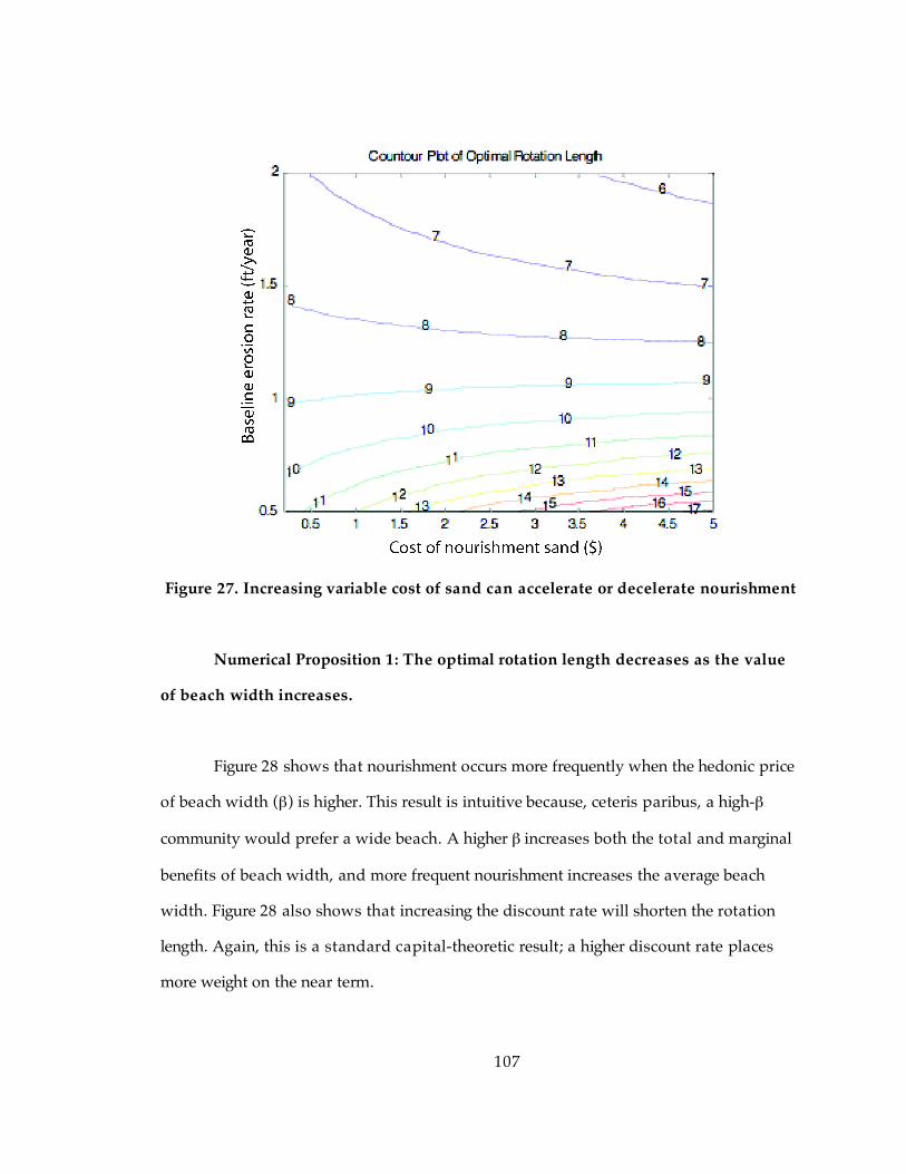
107
Figure 27. Increasing variable cost of sand can accelerate or decelerate nourishment
Numerical Proposition 1: The optimal rotation length decreases as the value
of beach width increases.
Figure 28 shows that nourishment occurs more frequently when the hedonic price
of beach width (β) is higher. This result is intuitive because, ceteris paribus, a high-β
community would prefer a wide beach. A higher β increases both the total and marginal
benefits of beach width, and more frequent nourishment increases the average beach
width. Figure 28 also shows that increasing the discount rate will shorten the rotation
length. Again, this is a standard capital-theoretic result; a higher discount rate places
more weight on the near term.

108
Figure 28. A higher value of beach width increases the frequency of nourishment
Numerical Proposition 2: The optimal rotation length decreases as the base
property value increases.
Figure 29 shows the intuitive result that communities will nourish more frequently
when the base property value (α) is higher. Again, increasing the discount rate will
shorten the rotation length. As population pressure in the coastal zone drives up coastal
property values, holding other features of the problem constant, our model predicts that
more beach nourishment will occur.

109
Figure 29. A higher base property value increases the frequency of nourishment
Numerical Proposition 3: The optimal rotation length decreases as the
baseline erosion rate increases.
Figure 30 illustrates this proposition. When the beach erodes faster, communities
must nourish more often to keep up.
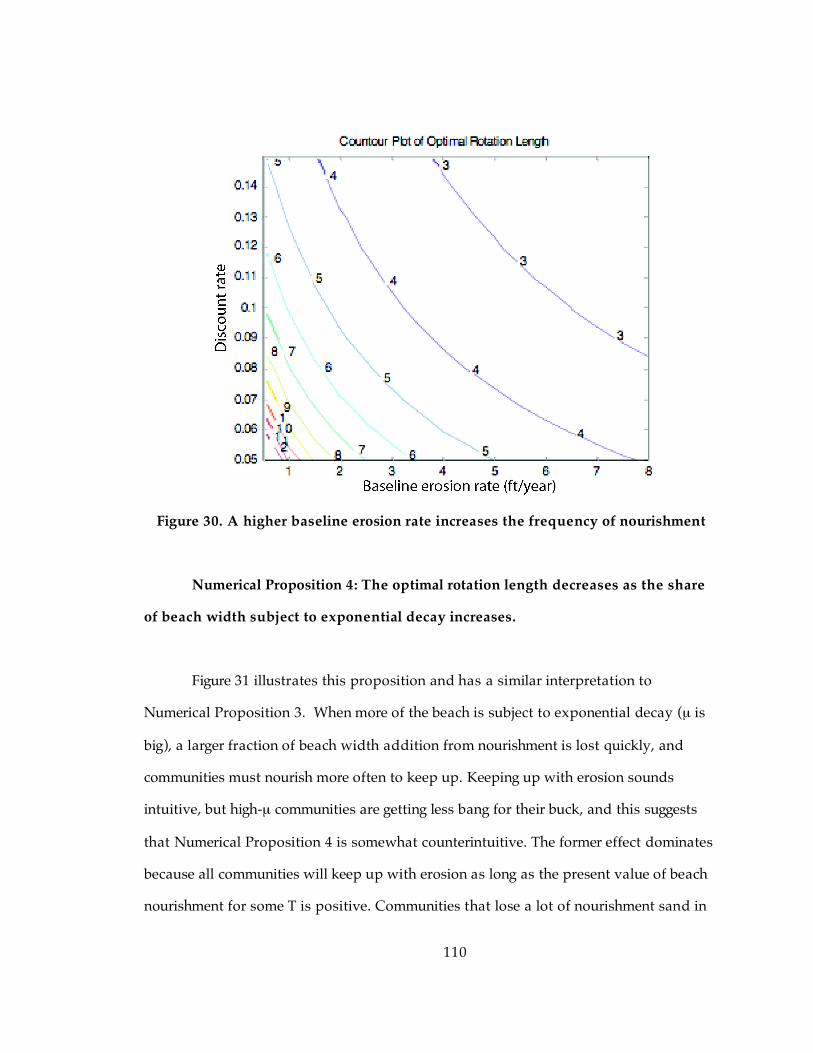
110
Figure 30. A higher baseline erosion rate increases the frequency of nourishment
Numerical Proposition 4: The optimal rotation length decreases as the share
of beach width subject to exponential decay increases.
Figure 31 illustrates this proposition and has a similar interpretation to
Numerical Proposition 3. When more of the beach is subject to exponential decay (µ is
big), a larger fraction of beach width addition from nourishment is lost quickly, and
communities must nourish more often to keep up. Keeping up with erosion sounds
intuitive, but high-µ communities are getting less bang for their buck, and this suggests
that Numerical Proposition 4 is somewhat counterintuitive. The former effect dominates
because all communities will keep up with erosion as long as the present value of beach
nourishment for some T is positive. Communities that lose a lot of nourishment sand in

111
the adjustment to equilibrium profile essentially become addicted to nourishment as a
beach stabilization strategy. In Figure 31, the present value of nourishment exceeds the
present value of abandoning the beach for all parameter value combinations, even
though the total present value of the optimal program—the solution to Equation 18,
v(T*)—is lower for high-µ communities than for low-µ communities. This is no different
than suggesting that two otherwise identical properties with different depreciation rates
will be priced differently in the market.
Figure 31. Frequency of nourishment increases with a higher share of beach width subject to exponential decay
Numerical Proposition 5: The optimal rotation length increases (decreases) as
the exponential decay rate of nourishment sand increases if the decay rate is higher
(lower) than the discount rate.

112
Figure 32 illustrates this proposition. The thick solid line is the 45-degree line
along which
!
" = # . Recall that in the traditional Faustmann problem—and the
interpretation due to Samuelson (1976)—the second term in the first order condition is
the foregone interest payment by delaying land rent, where land rent is the discounted
present value of all future rotations. A higher discount rate means that the difference
between marginal costs and marginal benefits of a single rotation must be greater to
compensate. To the left of the 45-degree line in Figure 32, the discount rate is higher than
the decay rate of nourishment sand. In other words, the depreciation of financial capital
(foregone interest) dominates the depreciation of sand capital. To balance interest lost
on land rent with marginal net benefits, the rotation length must decrease. The opposite
is true to the right of the 45-degree line where depreciation of sand capital dominates.
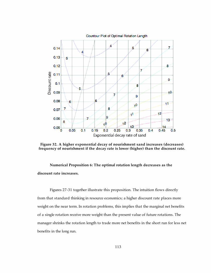
113
Figure 32. A higher exponential decay of nourishment sand increases (decreases) frequency of nourishment if the decay rate is lower (higher) than the discount rate.
Numerical Proposition 6: The optimal rotation length decreases as the
discount rate increases.
Figures 27-31 together illustrate this proposition. The intuition flows directly
from that standard thinking in resource economics; a higher discount rate places more
weight on the near term. In rotation problems, this implies that the marginal net benefits
of a single rotation receive more weight than the present value of future rotations. The
manager shrinks the rotation length to trade more net benefits in the short run for less net
benefits in the long run.

114
5.4 Discussion
Resource economics fundamentally deals with connections between natural
capital and financial capital. Optimal mineral extraction hinges on whether capital in
the bank grows faster than the value of capital in the ground. In fisheries and forestry,
optimal management entails balancing growth of the biological resource with growth of
the financial resource. When a managed beach is viewed as a renewable natural resource,
again we see this deep capital-theoretic connection. Optimal management from a beach
community’s perspective depends on the rates of decay of sand and financial capital. In
particular, the signs of two different comparative static results (Proposition 2 and
Numerical Proposition 5) hinge critically on whether
!
" < # . When nourishment sand
decays slower than the rate of foregone interest, an increase in variable cost or increased
nourishment sand decay could accelerate beach nourishment.
By focusing on a representative community, our model produces testable
hypotheses about real coastal communities in general. For empirical work, one would
need cross-community variation in erosion rates, base property values and values of
beach width (from hedonic studies), and records of nourishment activities. Such
empirical work is especially important for future research because actions of individual
communities could have consequences at the spatial scale of an entire coastline. That is,
small bumps in an otherwise uniform coastline can propagate over large spatial scales in
economically meaningful time scales (Ashton, Murray, and Arnoult 2001). If our positive
model describes real behavior, spatially heterogeneous property values and erosion rates
will lead to spatially heterogeneous nourishment interventions. Whether this process
would then lead to a more or less spatially uniform coastline than one that has not been
altered by humans is an open question.

115
A complementary approach to analyzing beach nourishment would be to use
numerical dynamic programming (Landry 2006). This approach allows for a more
general description of the state dynamics such that
!
˙ x (t) is a function of absolute time
and not just time since the last nourishment event. It also permits the choice of initial
beach width for each rotation. The drawbacks include increased computational burden
and the difficulty of generalizing comparative static or dynamic results. In our model, we
are able to obtain some analytical results before relying on numerical methods.
Nevertheless, with no previous literature on beach nourishment as a dynamic capital
accumulation problem and with increasing development pressure in the coastal zone, we
submit that our Faustmann-style rotation and numerical dynamic programming are both
worthwhile to pursue.
Although most of our model results conform to basic intuition, the possibility
that nourishment could increase in frequency as the variable costs increase is unsettling.
As sea level rises or storm patterns change in response to climate change, an increase in
the baseline erosion rate is not unlikely. At the same time, more people are living in the
coastal zone, and property values continue to rise. Nourishment sand that can be
recovered through dredging may eventually become scarce (Hoffman 1998), and one
would expect variable costs to increase. If communities respond by nourishing more
often, this effect could feed back on itself and further accelerate nourishment. Beaches
then become increasingly artificial, and the ecological costs of nourishment would grow
substantially. In the current policy regime, environmental impacts of nourishment are
cataloged but not counted as costs to weigh against nourishment benefits. In a future of
accelerated nourishment activity, policy-makers could begin to require these non-market
costs to be counted.
Our model does not address the funding mechanism for beach nourishment. We
implicitly assume that a dynamically optimal nourishment project—from the

116
community’s perspective— can be funded in some manner. Real projects receive funding
from federal, state, and local governments as well as private sources. Both the William J.
Clinton and George W. Bush administrations have supported reducing the federal share
of nourishment, though Congress passed the 2002 Water Appropriations Bill with $47.1
million more for beach nourishment than the $87.6 million that President Bush requested
(NOAA 2006). An important question for future research is how a change in the
availability of federal funds for nourishment will affect the prevalence and frequency of
nourishment. Conventional wisdom suggests that there would simply be less
nourishment, but our capital-theoretic model suggests that outcomes could be more
complicated. Whether a reduction in the federal share will increase or decrease
nourishment activity could depend on the allocation of federal funds across fixed and
variable costs.
117
References
Anderson, J., A. Rodriques, C. Fletcher, and D. Fitzgerald. 2001. Researchers focus attention on coastal response to climate change. Eos, Transactions American Geophysical Union 82, no. 44: 513.
Ashton, Andrew D. and A. B. Murray. 2006a. High-angle wave instability and emergent shoreline shapes: 1. Modeling of sand waves, flying spits, and capes. Journal of Geophysical Research 111 (F04011), doi:10/1029/2005JF000422.
----------. 2006b. High-angle wave instability and emergent shoreline shapes: 2. Wave climate analysis and comparisons to nature. Journal of Geophysical Research 111, F04012, doi:10.1029/2005JF000423.
Ashton, Andrew, A. Brad Murray, and Olivier Arnoult. 2001. Formation of coastline features by large-scale instabilities induced by high-angle waves. Nature 414 (15 November ), doi:10.1038/35104541: 296-300.
Ashton, Andrew, A. Brad Murray, and G. B. Ruessink. 2003. Initial tests of a possible explanation for alongshore sandwaves on the Dutch Coast. 3rd IAHR Symposium on River, Coastal and Estuarine Morphodynamics. International Association of Hydraulics Researchers. ISBN: 90-805649-6-6. Barcelona, Spain: 320-330
Ashton, Andrew, Jeffrey H. List, A. Brad Murray, and Amy S. Farris. 2003. Links between erosional hotspots and alongshore sediment transport. Proceedings of the International Conference on Coastal Sediments 2003. CD-ROM. World Scientific Publishing Corp. and East Meets West Productions. Corpus Christi, Texas, USA. ISBN 981-238-422-7.
Bell, F. W. and V. R. Leeworthy. 1990. Recreational demand by tourists for saltwater beach days. Journal of Environmental Economics and Management 18:189-205.
Brown, G. M. Jr. and H. O. Pollakowski. 1977. Economic valuation of shoreline. The Review of Economics and Statistics. 59: 272-278.
Brown, Katrina, Roger Few, Emma L. Tompkins, Mikis Tsimplis, and Tarja Sortti. 2005. Responding to climate change: inclusive and integrated coastal analysis. Tyndall Centre for Climate Change Research. Tyndall Centre project T2.42. Technical Report 24 (April).
Bruun, Per. 1962. Coastal erosion and the development of beach profiles, Journal of Waterways and Harbors Division 88: 117-130.
------------. 1983. Review of conditions for uses of the Bruun Rule of erosion. Coastal Engineering 7: 77-89.

118
Cowell, P, J., P. S. Roy, and R. A. Jones. 1995. Simulation of large-scale coastal change using a morphological behavior model. Marine Geology 126: 45-61.
Davidson-Arnott, R. G. D. and D. R. J. Langham. 2000. The effects of softening on nearshore erosion of a cohesive shoreline. Marine Geology 166: 145-162.
Dean, Robert G. 1988. Realistic economic benefits from beach nourishment. Proceedings of the 21st International Conference on Coastal Engineering. ASCE. Malaga, Spain: 1558-1572.
----------. 2002. Beach Nourishment: Theory and Practice. Hackensack: World Scientific.
Dean, Robert G. and Chul-Hee Yoo. 1992. Beach-nourishment performance predictions. Journal of Waterway, Port, Coastal and Ocean Engineering 118, no. 6 (November/December): 567-586.
Dean, Robert G. and E. M. Maurmeyer. 1983. Models for beach profile response. In: “Handbook of Coastal Processes and Erosion”, ed. Paul D. Komar and J. Moore. CRC Press. Boca Raton: 151-165.
Dickson, Mark E., Mike J. A. Walkden, and Jim W. Hall. 2007. Systemic impacts of climate change on an eroding coastal region over the twenty-first century. Climate Change 84, no. 2 (September), doi:10.1007/s10584-006-9200-9: 141-166.
Donahue, Kerry Anne, and Robert G. Dean. 1999. Sand size and fill geometry effects on longshore transport at a nourished beach. Coastal Sediments '99: Annual Symposium on Coastal Engineering and Science of Coastal Sediment Processes. CD-ROM. World Scientific. Hackensack, NJ.
Donnelly, Jeffrey P. and Jonathan D. Woodruff. 2007. Intense hurricane activity over the past 5,000 years controlled by El Niño and the West African monsoon. Nature 447 (24 May), doi:10.1038/nature05834: 465-468.
Dorfman, J. H., A. G. Keeler, and W. Kriesel. 1996. Valuing risk-reducing interventions with hedonic models: The case of erosion protection. Journal of Agricultural and Resource Economics 21, no. 1: 109-119.
Edwards, S. F. and F. J. Gable. 1991. Estimating the value of beach recreation from property values: An exploration with comparisons to nourishment costs. Ocean & Shoreline Management 15: 37-55.
Emanuel, Kerry. A. 1987. The dependence of hurricane intensity on climate. Nature 326 (08 April), doi:10.1038/326483a0: 483-485.
----------. 2005. Increasing destructiveness of tropical cyclones over the past 30 years, Nature 436 (4 August), doi:10.1038/nature03906: 686-688.
Falqués, A. and D. Calvete. 2005. Large-scale dynamics of sandy coastlines: diffusivity and instability, Journal of Geophysical Research 110 (C03007), doi:10.1029/2004JC002587.

119
Faustmann, M. 1849. Berechnung des Wertes welchen Waldboden sowie noch nich haubare Holzbestände für die Waldwirtschaft besitzen. Allgemeine Forst- und Jagd-Zeitung 15. Translated into English by W. Linnard and reprinted in Journal of Forest Economics 1: 7-44 (1995).
Geng, Quanzhen and Masato Sugi. 2003. Possible change of extratropical cyclone activity due to enhanced greenhouse gases and sulfate aerosols – study with a high resolution AGCM. Journal of Climate 16: 2262-2274.
Gornitz, Vivien. 1991. Global coastal hazards from future sea-level rise. Global and Planetary Change 89, no 3, doi:10.1016/0921-8181(91)90118-G: 379-398.
Grain, D. A., A. B. Bolton, and K. A. Bjorndal. 1995. Effects of beach renourishment on sea turtles: review and research inititiatives. Restoration Ecology 3: 95-104.
Haff, Peter K. 2007. The landscape Reynolds number and other dimensionless measures of Earth surface processes. Geomorphology 91 (3-4): 178-185, doi:10.1016/j.geomorph.2007.04.010.
Hallstrom, D. G. and V. K. Smith. 2005. Market responses to hurricanes. Journal of Environmental Economics and Management 50, no. 3: 541-561.
Hanson, Hans and N. C. Kraus. 1989. GENESIS: Generalized Model for Simulating Shoreline Change, Report 1: Technical Reference. Vicksburg: U.S. Army Engineering Waterways Experiment Station, Coastal Engineering Research Center.
Hartman, R. 1976. The harvesting decision when the standing forest has value. Economic Inquiry 14: 52-58.
Hoffman, C. W. 1998. Preliminary Assessment of Potential Sand Resource Areas Offshore of Nags Head, Kitty Hawk, and Kill Devil Hills, North Carolina. Report of the U.S. Minerals Management Service, State of North Carolina, Sand Resources Task Force.
Hooke, Roger LeB. 1994. On the efficacy of humans as geomorphic agents. GSA Today 4, no. 9: 217, 224-225.
Hooke, Roger LeB. 2000. On the history of humans as geomorphic agents. Geology 28, no:9: 843-846.
Houston, James R. 2002. The economic value of beaches – A 2002 update. Shore and Beach 70, no 1: 9-12.
Huang, J-C, G. R. Parsons, P. J. Poor, and M. Q. Zhao. 2004. Combining Conjoint Design and Travel Cost Model: Economic Analysis of Multi-Attribute Beach Erosion Control Programs. Working Paper. University of New Hampshire.
Intergovernmental Panel on Climate Change. 2007. Climate Change 2007: Impact, Adaptation, and Vulnerability—Contribution of Working Group II to the Fourth Assessment Report of the Intergovernmental Panel on Climate Change.

120
James, L. A. and W. A. Marcus. 2006. The human role in changing fluvial systems: Retrospect, inventory and prospect. Geomorphology 76: 152-171.
Komar, Paul D. 1971. The mechanics of sand transport on beaches. Journal of Geophysical Research 76, no 3 (January 20): 713-721.
Komar, Paul D. 1998. Beach Processes and Sedimentation. Upper Saddle River, New Jersey: Prentice Hall.
Komar, Paul D. and Douglas L. Inman. 1970. Longshore sand transport on beaches. Journal of Geophysical Research 75, no. 30 (October 20): 5914-5927.
Kriesel, Warren, Alan Randall, and Frank Lichtkoppler. 1993. Estimating the benefits of shore erosion protection in Ohio’s Lake Erie housing market. Water Resources Research 29, no. 4 (April), doi:10.1029/92WR02539: 795-802.
Lambert, Steven J. 1995. The effect of enhanced greenhouse warming on winter cyclone frequency and strengths. Journal of Climate 8 (May): 1447-1452.
Landry, Craig E. 2006. Optimal management of coastal erosion on developed barrier island beaches. Working Paper. Department of Economics, East Carolina University.
Landry, Craig E. 2007. Dynamic characteristics in hedonic property models. Working Paper. East Carolina University, Department of Economics.
Landry, Craig E., Andrew G. Keeler, and Warren Kriesel. 2003. An economic evaluation of beach erosion management alternatives. Marine Resource Economics 18: 105-127.
Landsea, Christopher. W. 2005. Hurricanes and global warming. Nature 438 (22/29 December), doi:10.1038/nature04477: E11-E12.
Larson, Magnus, and Nicholas C. Kraus. 1991. Mathematical modeling of the fate of beach fill. Coastal Engineering 16, no. 1: 83-114.
Larson, Magnus, Nicholas C. Kraus, and Mark R. Byrnes. 1990. SBEACH: numerical model for simulating storm-induced beach change; Report 2, Numerical formulation and model tests. Vicksburg: U. S. Army Engineering Waterways Experiment Station, Coastal Engineering Research Center.
Lazarus, Eli D., and A. Brad Murray. 2007. Process signatures in regional patterns of shoreline change on annual to decadal time scales. Geophysical Research Letters 34, no. 19 (L19402), doi:10.1029/2007GL031047.
Le Mehaute, Bernard and Mills Soldate. 1979. Mathematical modeling of shoreline evolution. in Proceedings of the 16th Coastal Engineering Conference. 1163-1179. New York: American Society of Civil Engineers.
List, Jeffrey H. and Amy S. Farris. 1999. Large-scale shoreline response to storms and fair weather, in Drause, N. C., and McLougal, W. G. Coastal Sediments ’99: Annual Symposium on Coastal Engineering and Science of Coastal Sediment Processes. CD-ROM. World Scientific. Hackensack, NJ.

121
McNamara, D. and B. Werner. Coupled barrier island-resort model: 1. Emergent instabilities induced by strong human-landscape interactions. In press at Journal of Geophysical Research – Earth Surface.
McNamara, D. and B. Werner. Coupled barrier island-resort model: 2. Tests and predictions along Ocean City and Assateague Island National Seashore, Maryland. In press at Journal of Geophysical Research – Earth Surface.
McNinch, Jesse E. 2004. Geologic control in the nearshore: shore-oblique sandbars and shoreline erosional hotspots, Mid-Atlantic Bight, USA. Marine Geology 211, issues 1-2 (30 September): 121-141.
McNinch, Jesse E. and John T. Wells. 1999. Sedimentary processes and depositional history of a cape-associated shoal, Cape Lookout, North Carolina. Marine Geology 158: 233-252.
McNinch, Jesse E. and Richard A. Leuttich, Jr. 2000. Physical processes around a cuspate foreland headland: implications to the evolution and long-term maintenance of a cape-associated shoal. Continental Shelf Research 20, no. 17 (15 December): 2367-2389.
Milon, W. J., Gressel, J., and David Mulkey. 1984. Hedonic amenity valuation and functional form specification. Land Economics 60, no. 4: 378-387.
Miselis, Jennifer L. and Jesse E. McNinch. 2006. Calculating shoreline erosion potential using nearshore stratigraphy and sediment volume: Outer Banks, North Carolina. Journal of Geophysical Research 111 (F02019), doi:10.1029/2005JF000389.
Murray, A. Brad and Andrew Ashton. 2003. Sandy-coastline evolution as an example of pattern formation involving emergent structures and interactions. Proceedings of the International Conference on Coastal Sediments 2003. CD-ROM. World Scientific Publishing Corp. and East Meets West Productions. Corpus Christi, Texas, USA. ISBN 981-238-422-7.
Murray, A. Brad and Andrew Ashton. 2004. Extending a 1-line modeling approach to explore emergent coastline behaviors. Proceedings of the 29th International Conference on Coastal Engineering. ASCE. Lisbon, Portugal. 2035-2047.
Murray, A. Brad, Lisa Valvo, Jordan Slott, Andrew Ashton, and Thomas Crowley. 2007. Variable shoreline responses to sea-level rise and climate change. In: “Coastal Sediments 2007: 6th International Symposium on Coastal Engineering and Science of Coastal Sediment Processes” ed. Nicholas C. Kraus and Julie Dean Rosati. ASCE. (15 May). New Orleans, LA.
National Oceanic and Atmospheric Administration (NOAA). 2006. Coastal Services Center, Beach Nourishment: A Guide for Local Government Officials. http://www.csc.noaa.gov/beachnourishment/html/human/socio/geodist.htm and http://www.csc.noaa.gov/beachnourishment/html/human/socio/change.htm, (accessed November 26, 2006).

122
National Research Council (NRC). 1995. Beach Nourishment and Protection, Washington DC: National Academy Press.
Parsons, George R. and Michael Powell. 2001. Measuring the cost of beach retreat. Coastal Management 29: 91-103.
Parsons, George R. and Ynagru Wu. 1991. The opportunity cost of coastal land-use controls: an empirical analysis. Land Economics, 67, no. 3: 308-316.
Peldnard-Considere, R. 1956. Essai de theorie de l’evolution des formes de rivage en plages de sable et de galets. 4th Journees de l’Hydraulique, Les Energies de al Mer. Question III. Rapport No. I: 289-298.
Pielke, Jr. Roger. A. 2005. Are there trends in hurricane destruction? Nature 438 (22/29 December), doi:10.1038/nature04426: E11.
Pilkey, O. H. and T. D. Clayton. 1987. Beach replenishment: the national solution?. Coastal Zone ’87. ASCE. Seattle, WA.
Pilkey, Orrin H. Jr., and Howard L. Wright III. 1988. Seawalls versus beaches. In: “The Effects of Seawalls on the Beach” ed. Krause, Nicholas C. and Orrin H. Pilkey, Jr. Special Issue, Journal of Coastal Research 4: 41-64.
Pilkey, Orrin H., William J. Neal, Stanley R. Riggs, Craig A. Webb, David M. Bush, Deborah F. Pilkey, Jane Bullock, and Brian A. Cowan. 1998. The North Carolina shore and its barrier islands: restless ribbons of sand. Durham: Duke University Press.
Pompe, Jeffrey J. and James R. Rinehart. 1994. Estimating the effect of wider beaches on coastal housing prices. Ocean & Coastal Management 22: 141-152.
Pompe, Jeffrey J. and James R. Rinehart. 1995. The value of beach nourishment to property owners: storm damage reduction benefits. Review of Regional Studies 25, no. 3: 271-285.
Reolvink, J. A. and G. K. F. M. Van Banning. 1994. Design and development of Delft3D and application to coastal morphodynamics. Proc. of Hydroinformations ’94 conference, Delft.
Samuelson, P.A. 1976. Economics of forestry in an evolving society. Economic Inquiry 14: 466-492.
Silberman, J., D. Gerlowski, and N. Williams. 1992. Estimating existence values for users and nonusers of New Jersey beaches. Land Economics 68: 225-236.
Slott, Jordan M., A. Brad Murray, Andrew D. Ashton, and Thomas J. Crowley. 2006. Coastline responses to changing storm patterns. Geophysical Research Letters 33 (L18404), doi:10.1029/2006GL027445.
123
Spatial Trends in Coastal Socioeconomics (STICS). Coastal Zone Country Facts: Draft. http://marineeconomics.noaa.gov/socioeconomics/CZCounties/ cz_pop_housing/cz_county_mainpage.html (accessed 21 February 2007).
Syvitski, J. P. M., C. J. Vörösmarty, A. J. Kettner, and P. Green. 2005. Impact of humans on the flux of terrestrial sediment to the global coastal ocean. Science 308: 376-380, doi:10.1126/science.1109454.
Taylor, L.O. and V.K. Smith. 2000. Environmental amenities as a source of market power. Land Economics 76, no. 4:550-568.
Titus, James T., Richard A. Park, Stephen P. Leatherman, J. Richard Weggel, Michael S. Greene, Paul W. Mausel, Scott Brown, Gary Gaunt, Manjit Trehan, and Gary Yohe. 1991. Greenhouse effect and sea level rise: The cost of holding back the sea. Coastal Management 19: 171-204.
Trembanis, Arthur. C. and Orrin H. Pilkey. 1998. Summary of beach nourishment along the U.S. East Gulf of Mexico shoreline. Journal of Coastal Research 14, no. 2: 407-417.
U.S Army Corps of Engineers. 2002. Final feasibility report and environmental impact statement on hurricane protection and beach erosion control: Dare Country beaches, Volume 1. Wilmington District, South Atlantic Division, Dare County, NC.
U.S. Climate Change Science Program. 2001. The potential consequences of climate variability and change on coastal areas and marine resources. http://www.usgcrp.gov/usgcrp/nacc/coasts/default.htm (accessed February 14, 2008).
U.S. Congress. House. 2002. Water Resources Development Act of 2002. HR 5428. 107th Cong., 2nd sess., Congressional Record 148, daily ed. (September 23): H 6473.
Valverde, Hugo. R., Arthur C. Trembanis, and Orrin H. Pilkey. 1999. Summary of beach nourishment episodes on the U.S. East coast barrier islands. Journal of Coastal Research 15, no 4 (Fall): 1100-1118.
Valvo, Lisa M., A. Brad Murray, and Andrew Ashton. 2006. How does underlying geology affect coastline change? An initial model investigation. Journal of Geophysical Research 111 (F02025), 10.1029/2005JF000340.
Water Resources Development Act of 1986. Public Law 99-662. 99th Cong., 2d sess. November 17.
Water Resources Development Act of 1999. Public Law 106-53. 106th Cong., 1st sess. August 17.
Webster, P. J., G. J. Holland, J. A. Curry, and H.-R. Chang. 2005. Changes in tropical cyclone number, duration, and intensity in a warming environment. Science 309 (16 September): 1844-1846.

124
Werner, B. and D. McNamara. 2007. Dynamics of coupled human landscape systems. Geomorphology 91: 393-407.
Witham, Ross. 1989. Beach preservation and sea turtle nesting. In: Proceedings Beach Preservation Technology ’89: Strategies and Alternatives in Erosion Control. Tampa, Florida, 22-24 February: 143-146.
Woglom, Emily. 2003. The dynamics of shoreline management: an approach using renewable resource economics. Unpublished Masters Project, Nicholas School of the Environment and Earth Sciences, Duke University.
Work, Paul. A. and W. Erick Rogers. 1998. Laboratory study of beach nourishment behavior. Journal of Waterway, Port, Coastal, and Ocean Engineering 124, no. 5 (September/October): 229-237.
Yohe, G., J. Neumann, and H. Ameden. 1995. Assessing the economic costs of greenhouse-induced sea level rise: methods and application in support of a national survey. Journal of Environmental Economics and Management 29: S78-S97.
Zhang, Keqi, Bruce C. Douglas, and Stephen P. Leatherman. 2000. Twentieth-century storm activity along the U. S. East Coast, Journal of Climate 13, no. 10: 1748-1761.
----------. 2004. Global warming and coastal erosion. Climate Change 64, no. 1-2 (May), doi:10.1023/B:CLIM. 0000024690.32682.48: 41-58.
125
Biography
Jordan Matthew Slott was born in New York, NY, USA on June 14, 1973. He
received a Bachelor of Science in Computer Science and Engineering and a Masters of
Engineering in Electrical Engineering and Computer Science in June 1996 from the
Massachusetts Institute of Technology, Cambridge, MA, USA. He is a member of the Eta
Kappa Nu Electrical Engineering Honor Society and the Sigma Xi Scientific Research
Society. Jordan was awarded the James B. Duke Fellowship in 2004 from Duke
University. Jordan’s list of publications includes:
Slott, Jordan M., A. Brad Murray, Andrew D. Ashton, and Thomas J. Crowley. 2006. Coastline responses to changing storm patterns. Geophysical Research Letters 33 (L18404), doi:10.1029/2006GL027445.
Slott, Jordan M. Martin D. Smith, and A. Brad Murray. 2008. Synergies between
adjacent beach-nourishment communities in a Morpho-economic coupled coastline model. In Press at Coastal Management Journal.
Murray, A. Brad, Lisa Valvo, Jordan Slott, Andrew Ashton, and Thomas Crowley.
2007. Variable shoreline responses to sea-level rise and climate change. In: “Coastal Sediments 2007: 6th International Symposium on Coastal Engineering and Science of Coastal Sediment Processes” ed. Nicholas C. Kraus and Julie Dean Rosati. ASCE. (15 May). New Orleans, LA.