numerical simulation of liquid sloshing in a partially ﬁlled...

Numerical simulation of liquid sloshing in a partially filled containerwith inclusion of compressibility effects

Y. G. Chena� and W. G. Priceb�

School of Engineering Sciences, Ship Science, University of Southampton,Southampton SO17 1BJ, United Kingdom

�Received 8 July 2009; accepted 14 October 2009; published online 19 November 2009�

A numerical scheme of study is developed to model compressible two-fluid flows simulating liquidsloshing in a partially filled tank. For a two-fluid system separated by an interface as in the case ofsloshing, not only a Mach-uniform scheme is required but also an effective way to eliminateunphysical numerical oscillations near the interface. By introducing a preconditioner, the governingequations expressed in terms of primitive variables are solved for both fluids �i.e., water, air, gas,etc.� in a unified manner. In order to keep the interface sharp and to eliminate unphysical numericaloscillations in unsteady fluid flows, the nonconservative implicit split coefficient matrix method ismodified to construct a flux-difference splitting scheme in the dual-time formulation. The proposednumerical model is evaluated by comparisons between numerical results and measured data forsloshing in an 80% filled rectangular tank excited at resonance frequency. Through similarcomparisons, the investigation is further extended by examining sloshing flows excited by forcedsway motions in two different rectangular tanks with 20% and 83% filling ratios. These examplesdemonstrate that the proposed method is suitable to capture induced free surface waves and toevaluate sloshing pressure loads acting on the tank walls and ceiling. © 2009 American Institute ofPhysics. �doi:10.1063/1.3264835�

I. INTRODUCTION

The effect of dispersed bubbles or entrapped air in atwo-fluid sloshing flow is important when the excited surfacewave impacts on the sides or roof of a container.1 When awave breaks or is near to breaking as it hits a wall, air oftenbecomes trapped. The presence of air as a trapped bubble ordispersed air, or most likely a combination of both, has acushioning effect and local pressures are then influenced bythe compressibility of the air.2–4 Therefore, investigations ofcompressibility effects of gas and liquid in violent sloshingmotions provide improved insights and understanding of thecomplicated hydrodynamic phenomena occurring in high-speed impacts on tank walls, air bubble entrapment, breakingwaves, and so on.

To compute compressible multifluid flows arising in liq-uid sloshing in a partially filled moving tank, there are twomajor issues that need resolving. The first requires the devel-opment of a unified method to solve conditions varying fromweakly compressible flows to high-speed flows. The standardmethods adopted to solve compressible flows based on thehyperbolic conservation laws are neither numerically robustnor efficient in the case of low Mach number or weak com-pressibility �the incompressible limit�.5–7 For many algo-rithms preconditioning techniques are a necessity in order toobtain a converged solution at low speeds.7–11 Another issueis that for any standard conservative, shock-capturing

scheme to compute multifluid systems, pressure oscillationsexist intrinsically near the interface surface.12,13 In a com-pressible two-fluid flow computation, pressures �densities�are used for further computations, such as the computation ofdensities �pressure� from their equations of state, which giverise to numerically based oscillations near the interface andfinally cause deterioration of the whole flow field at subse-quent times. Such oscillations are present in first-order com-putations and do not decrease with decreasing the mesh sizein any interface capturing method other than a trackingmethod.14 The interfacial correction method based on an ex-act Riemann solver proposed by Cocchi et al.,15 Davis,16 andIgra,17 locally nonconservative fixes suggested by Abgrall18

and the ghost fluid method introduced by Fedkiw et al.19 arethe best known approaches to overcome the described diffi-culties.

In this study, a preconditioner is introduced to solve mul-tifluid flows in a unified manner. The present approach com-bines the preconditioning technique with an implicit splitcoefficient matrix method �SCMM� scheme to ensure thegeneration of a numerical method applicable to both incom-pressible and compressible flow regimes and devoid of nu-merically induced pressure oscillations near the interface.This requires the application of a dual-time preconditioningtechnique11 to the two-fluid flows. A characteristic-basedprimitive-variable flux-difference splitting method related tothe SCMM scheme20 is employed to reduce interface diffu-sion and eliminate numerical spurious oscillations with thelevel set approach adopted to capture the free surfacecharacteristic.21

a�Author to whom correspondence should be addressed. Telephone: �448059 6524. Fax: �44 8059 3299. Electronic mail: [email protected].

b�Electronic mail: [email protected].

PHYSICS OF FLUIDS 21, 112105 �2009�

1070-6631/2009/21�11�/112105/16/$25.00 © 2009 American Institute of Physics21, 112105-1

Downloaded 22 Dec 2009 to 152.78.32.146. Redistribution subject to AIP license or copyright; see http://pof.aip.org/pof/copyright.jsp

http://dx.doi.org/10.1063/1.3264835

http://dx.doi.org/10.1063/1.3264835

http://dx.doi.org/10.1063/1.3264835

II. THEORETICAL FORMULATION

A. Three-dimensional governing equations

The fluid motion in liquid and gas phases are both as-sumed to be compressible. This two-fluid system is assumedimmiscible and adiabatic, and fluid density � is only a func-tion of pressure p, e.g., �=��p�. The basic equations describ-ing the two-fluid system are expressed in Cartesian coordi-nates as

��

�t+

��uj��xj

= 0, �1�

��ui��t

+��ijp�

�xj+

��uiuj��xj

−�

�xj�2�

Resij� = −

�gi

Fn2 − �f i.

�2�

A conventional Cartesian tensor notation is adopted inthese two equations. The spatial coordinates xi �i=1,2 ,3�,velocity components ui, and projection components of thegravitational acceleration in the axis directions gi, respec-tively, have been nondimensionalized for each specific prob-lem in terms of a characteristic length L, a characteristicvelocity U0, and gravitational acceleration g. The fluid den-sity � and viscosity � are nondimensionalized by their re-spective water reference values �w and �w at a prescribedstate; the time t and the pressure p variables are nondimen-sionalized by L /U0 and �wU0

2, respectively. The Reynoldsnumber, Re, Froude number, Fn, and strain rate tensor sij aredefined by

Re = LU0/�w, Fn = U0/�Lg ,

�3�

sij =1

2� �ui

�xj+

�uj

�xi� .

With the exception of the gravitational force, the exter-nal forces include the translational and rotational inertiaforces, and f i takes the following form:

f i = ai + �ijkd� j

dtxk + �ijk�klm� j�lxm + 2�ijk� juk, �4�

where ai represents the translational acceleration componentsand �i represents the rotational angular velocity components.Here �ijk denotes the Levi-Civita symbol with repeating sub-scripts indicating summation. The effect of surface tension isneglected in this mathematical model.

To simulate fluid sloshing problems encountered in thefield of ship hydrodynamics, the gas and liquid are both as-sumed adiabatic and their thermodynamic behavior is de-scribed by an equation of state. For example, the Tait equa-tion of state14 is employed for water and the ideal gasequation of state for air is used with different parameter val-ues. They have the following unified form:

p + B

p0 + B= � �

�0��

, �5�

where p0 and �0 are the reference pressure and density val-ues, respectively. For example, for water, the constants B and

� are given by Bw=296.310+6 and �w=7.415, and for airby Ba=0 and �a=1.4. In terms of Eq. �5�, the speed of soundfor each fluid phase is calculated from the following equa-tion:

c =��p

��=��B + p�

�.

B. Free surface capturing method

The free surface is defined as the zero level set of a levelset function initialized as a signed distance function fromthe interface. In air, is set to a positive value and in waterto a negative value as defined by

��x1,x2,x3;t� � 0 in air,

�x1,x2,x3;t� = 0 on surface,

�x1,x2,x3;t� � 0 in water. �6�

Differentiating =0 with respect to time t, a transportequation is derived to describe the free surface motion in theform

�

�t+ ui

�

�xi= 0, �7�

where ui is the local fluid velocity and, at any time, movingthe interface is equivalent to updating by solving Eq. �7�.

Due to the sharp change in properties of fluids at theinterface, we introduce a region of finite thickness overwhich a smooth but rapid change in density and viscosityoccurs across the interface.

First, we define a smoothed Heaviside function H��x�satisfying

H��x� = � 1 if x � � ,

0 if x � − � ,

0.5�x + ��/� + 0.5 sin� x/��/ otherwise,�8�

where � is half the finite thickness of the interface in whichthe density and viscosity change.22

Using the above function, we can define the correspond-ing smoothed viscosity function � as

�� = �1 − H�� +�a

�wH�� . �9�

The density is updated by means of the equation of state. Thetwo nondimensional densities �1= �p / �p0+Bw�+1�1/�w and�2=�a /�w��p / p0�+1�1/�a are evaluated from Eq. �5� using thepressure value at a grid point and the correspondingsmoothed density function � is defined as

�� = �1�1 − H�� + �2H�� , �10�

where the constant Bw and reference pressure p0 are nondi-mensional quantities. The gauge pressure �i.e., the referencepressure subtracted from the absolute pressure� is used inorder to reduce the effect of round-off errors at low speedfluid flows.

112105-2 Y. G. Chen and W. G. Price Phys. Fluids 21, 112105 �2009�


Even if we initialize as a signed distance from a wavefront, the level set function no longer remains a distancefunction at later times. For numerical reasons, the level setfunction is reinitialized so that satisfies �=1. An itera-tive procedure is used at each time step22 by solving thefollowing Hamilton–Jacobi equation:

�

�t= sgn�0��1 − �� ,

�11��x1,x2,x3;t� = 0�x1,x2,x3� ,

where sgn denotes the sign function. Given a level set func-tion, 0, at time t, the previous equation has the property thatthe steady state solution has the same sign and same zerolevel set as 0, and converges to �=1. Therefore, it is adistance function to the wave front. For numerical reasons,22

this sign function is approximated by

S��0� =0

�02 + �2

.

During the reinitialization exercise a numerical proce-dure developed by Sussman et al.23 was introduced to pre-serve the fluid volume in each cell to improve the accuracyof solution of Eq. �11�. In the numerical experiments de-scribed in Sec. IV, this improved level set method23 wasadopted and it produced a significant improvement to theaccuracy of capturing free surface waves.

C. Preconditioning dual-time technique

In solving the compressible equations for low Machnumber, the acoustic eigenvalues are much higher than theconvective ones. For the sake of stability the time step incre-ment must be chosen inversely proportional to the highesteigenvalue of the system to satisfy the Courant–Friedrichs–Lewy condition.24 This implies that other waves convected atfluid speed do not change very much over a time step andthousands of time steps may be required for them to reach asteady state value. Hence, the standard methods for com-pressible flows based on the hyperbolic conservation lawsare neither numerically robust nor efficient in the case of lowMach number or weak compressibility.

In this study, primitive variables, rather than conserva-tive variables, are employed to evolve time-dependentReynolds-Averaged Navier–Stokes equations. The precondi-tioning technique developed for compressible single phaseflows by changing the eigenvalues of the system7,11 is ex-tended to compressible two-fluid flow problems associatedwith liquid sloshing in partially filled containers. An impor-tant feature of the proposed method is that the compressiblegas and liquid equations are unified to a single system, e.g.,a single phase flow, and in each time step both phases areupdated simultaneously. The interface is only treated as avariation in fluid properties.

In terms of generalized coordinates, Eqs. �1� and �2�with the addition of a preconditioned pseudotime derivativecan be rewritten in a vector form as given by

��

�q

��+

�Q

�t+

�Fj

�� j+

�Fj�

�� j= S , �12�

where vectors q, Q, Fj, Fj�, and S are expressed as

q = J−1�p,u,v,w�T, Q = J−1��,��u,��v,��w�T,

Fj = J−1��Uj

��u1Uj +�� j

�x1p

��u2Uj +�� j

�x2p

��u3Uj +�� j

�x3p� ,

Fj� = J−1 ��

Re

�� j

�xm�0,

��k

�xm

�u

��k+

��k

�x

�um

��k,��k

�xm

�v��k

+��k

�y

�um

��k,��k

�xm

�w

��k+

��k

�z

�um

��k�T

,

S = J−1��0, f1 + g1/Fn2, f2 + g2/Fn2, f3 + g3/Fn2�T.

Here J=�� ,� ,�� /��x ,y ,z� is the Jacobian of the transforma-tion and the contravariant velocity component Uj is definedas

Uj =�� j

�xmum.

To optimize the performance of the pseudoiteration, thepseudotime term is written in terms of the primitive vari-ables. The preconditioning step consists of the replacementof matrix �� by a matrix defined by

�� = �1/Vr

2 0 0 0

u/Vr2 �� 0 0

v/Vr2 0 �� 0

w/Vr2 0 0 ��

� .

Here, Vr is the reference velocity which is chosen to ensurethat the system is well conditioned at low speed and to ac-celerate convergence. In practice, this parameter is generallydefined as some functional combination of the free streamand the local convective velocities.7,11

III. NUMERICAL METHOD

The implementation of the preconditioned dual-time al-gorithm is now discussed adopting two different discretiza-tion strategies. The conservative Roe’s flux-difference split-ting method25 is presented to solve the compressible singlephase fluid flow, whereas the nonconservative SCMM or ahybrid combining both schemes of presentation is used forthe compressible two-fluid flow.

For the sake of simplicity in Sec. III A, only the convec-tive flux derivative in one direction is presented, and theviscous and source terms in Eq. �12� are omitted. For ex-ample, we denote by F the convective flux F1 in the�-direction.

112105-3 Numerical simulation of liquid sloshing Phys. Fluids 21, 112105 �2009�


A. Preconditioned Roe’s flux-difference formulations

First let us consider Roe’s approximate Riemannscheme,25 which is given by

Fj+1/2 = 12 �F�Qj+1/2

L � + F�Qj+1/2R � − A�Qj+1/2

L ,Qj+1/2R �

�Qj+1/2R − Qj+1/2

L �� . �13�

Roe’s method provides an exact solution to an approximateRiemann problem by evaluating the Jacobian matrix A of theconvective flux vector F as Roe-averaged variables depen-dent on left and right states Qj+1/2

L and Qj+1/2R at the interface

�=� j+1/2. In this expression, A=T�T−1, where T is the ma-trix whose columns are the right eigenvectors of A, T−1 is thematrix whose rows are the left eigenvectors of A, and � isa diagonal matrix whose elements are the absolute values ofthe eigenvalues of A.

By implicitly discretizing Eq. �12� with a first-order fi-nite difference scheme for the pseudotime and a second-order backward difference approximation for the physicaltime terms, we have

��

qm+1,n+1 − qm,n+1

��+

1.5Qm+1,n+1 − 2Qn + 0.5Qn−1

�t

+ ��Fm+1,n+1 = 0. �14�

Here, the superscript n denotes the nth physical time level,the superscript m the level of the subiteration, and �� repre-sents a spatial difference. After linearizing terms at the �m+1�th time level and involving some simple algebraic ma-nipulation, the above equation becomes

�� + M3��

2�t+ Aq��q + ��F

m,n+1 = rm,n+1, �15�

where �� represents the pseudotime difference, and Aq

=�F /�q, M =�Q /�q, and

rm,n+1 = −1.5Qm,n+1 − 2Qn + 0.5Qn−1

�t.

Let us define �d=��+M�3�� /2�t� as the nonconserva-tive variable preconditioning matrix. Multiplying both sidesof Eq. �15� by the inverse �d

−1, we derive the result

�I + aq��q + aq��q = �d−1r , �16�

where it is easily verified that the preconditioned flux Jaco-bian matrix and the Roe numerical flux expression in termsof primitive variables are, respectively, given by

aq = �d−1Aq,

�17�Fj+1/2 = 1

2 �FL + FR� − 12 �daq�q .

Here the tilde over each term means that they are evaluatedusing the Roe-averaged variables.

Furthermore, the transformation of Eq. �16� into conser-vative variables gives

�I + a��Q + a��Q = M�d−1r . �18�

It now follows that the system matrix for the vector Q isgiven by

a = MaqM−1 = M�d−1AqM−1 = M�d

−1A

and the corresponding numerical flux at a cell interface,analogous to Eq. �17�, is defined as

Fj+1/2 = 12 �FL + FR� − 1

2 �dM−1a�Q , �19�

where the matrix �dM−1 is defined as the conservative vari-able preconditioning matrix.

Since Eqs. �16� and �18� with the corresponding Roe’snumerical fluxes in Eqs. �17� and �19� are equivalent, the twomethods described here are conservative but do not satisfythe discrete Rankine–Hugoniot jump conditions to ensure ex-act recognition of isolated discontinuities such as a shockwave.

B. Preconditioned SCMM formulation

The basic idea behind the nonconservative SCMMscheme26 is to split the Jacobian coefficient matrix into twosubmatrices, each associated with the positive or negativeeigenvalues of the Jacobian. Hence, a one-sided finite differ-ence scheme can be applied to each split flux difference.

The multiplication of both sides of Eq. �16� by �d andimplementing the similarity transform for the Jacobian ma-trix aq=T�T−1 leads to

��d + ��dT�T−1��q + �dT�T−1��q = r . �20�

Here the diagonal matrix � consists of the eigenvalues of aq

and T is the matrix of its right eigenvectors.The implementation of positive and negative decompo-

sition of the Jacobian matrix and by defining the positive andnegative nonconservative flux differences as

��F+ = �dT�+T−1��q = �daq

+��q = aq+��q ,

��F− = �dT�−T−1��q = �daq

−��q = aq−��q

allow Eq. �20� to be expressed in the form

��d + ��a+�� + ��a−��q = r − ��F+ − ��F

−, �21�

where the plus �minus� eigenvalue matrices are given by

�� = 12 �� .

The first-order upwind difference approximation to thepositive and negative flux differences at a node j is

��F+ + ��F

− aq+�qj−1/2��qj − qj−1� + aq

−�qj+1/2��qj+1 − qj� ,

�22�

where qj+1/2 is the arithmetic average of the primitive vari-ables qj and qj+1.

Higher order spatial discretizations were derived byLombard et al.26 For example, the second-order upwind andthird order upwind-biased methods are defined, respectively,by



32 aq

+�qj−1/2��q − 12 aq

+�qj−3/2��q + 32 aq

−�qj+1/2��q

− 12 aq

−�qj+3/2��q �23�

and

13 aq

+�qj+1/2��q + 56 aq

+�qj−1/2��q − 16 aq

+�qj−3/2��q

+ 13 aq

−�qj−1/2��q + 56 aq

−�qj+1/2��q − 16 aq

−�qj+3/2��q .

�24�

The SCMM scheme based on the primitive variables asdescribed, although it eliminates numerical spurious oscilla-tions near the interface, is nonconservative. This implies thatthis numerical scheme of study can only be applied to lowMach number flows, transonic flow, or to a problem involv-ing the simultaneous presence of both.

C. Eigensystem and numerical convective fluxes

The nonconservative variable preconditioning matrix �d

in Eqs. �16� and �20� has the form

�d = �� +3��

2�tM = �

b1 0 0 0

ub1 b2 0 0

vb1 0 b2 0

wb1 0 0 b2

� , �25�

where b1= �1 /Vr2�+ �1.5�� /�t��1 /c2� and b2=��1

+ �1.5�� /�t��.The preconditioned inviscid flux Jacobian matrix aq in

Eqs. �16� and �20� is expressed as

aq = �d−1Aq = �

U1/�c2b1� ��

��

�x/b1 ��

��

�y/b1 ��

��

�z/b1

��

�x/b2 ��U1/b2 0 0

��

�y/b2 0 ��U1/b2 0

��

�z/b2 0 0 ��U1/b2

��26�

and its eigenvalues are given by

�1 = �2 = ��U1/b2,

�27�

�3,4 =��U1

2� 1

b2+

1

��c2b1� ��U1

2b2�2

+��

b1b2

��

�xj

��

�xj+ � U1

2c2b1�2

−��U1�2

2c2b1b2�

��U1

2� 1

b2+

1

��c2b1� � � .

The eigenvectors associated with the four eigenvalues used in Eq. �20� are expressed as

T = �0 0

�3 − ��U1/b2

2�

�4 − ��U1/b2

2�

�x

��

�x

��

1

2�b2

��

�x

1

2�b2

��

�x

�y

��

�y

��

1

2�b2

��

�y

1

2�b2

��

�y

�z

��

�z

��

1

2�b2

��

�z

1

2�b2

��

�z

� .

The inverse of the matrix T is of the form

T−1 =1

T�0

��

2�b22� �y

��

��

�z−

�z

��

��

�y� ��

2�b22� �z

��

��

�x−

�x

��

��

�z� ��

2�b22� �x

��

��

�y−

�y

��

��

�x�

0��

2�b22� �z

��

��

�y−

�y

��

��

�z� ��

2�b22� �x

��

��

�z−

�z

��

��

�x� ��

2�b22� �y

��

��

�x−

�x

��

��

�y�

Tb2

��

−�4 − ��U1/b2

2�

��

�x−

�4 − ��U1/b2

2�

��

�y−

�4 − ��U1/b2

2�

��

�z

−Tb2

��

�3 − ��U1/b2

2�

��

�x

�3 − ��U1/b2

2�

��

�y

�3 − ��U1/b2

2�

��

�z

� ,



where T= �� /2�b22�� /�xj�� /�xj��0.

The numerical flux �F1� j+1/2,k,l in the �-direction for thethree dimensional case is given by Eqs. �22� and �23�, or Eq.�24� in terms of different spatial accuracies. The numericalfluxes in the other two directions can be calculated similarlyin terms of the directional split method.24

It is noticed that after adding a preconditionedpseudotime derivative term �the first term� to the originalsystem in Eq. �12� and moving the difference approximationof the physical time derivative term to the hand right side asa source term in Eq. �15�, the time derivative preconditionedsystem of equations constructed here is now hyperbolic inpseudotime �. The physical time coordinate is used to trackthe physical variation of the flow, whereas the pseudotimecoordinate is used to march this system to a steady state ateach physical time step. It is seen that Eq. �21� is expressedin an incremental form based on the flow variable differencebetween iterations �q=qn+1,m+1−qn+1,m. Therefore, providedthe solution converges in pseudotime �i.e., �q→0 as m→��, the left-hand side term goes to zero and the computedsolution satisfies the original governing equations. In thisstudy, the preconditioning methods are constructed to accel-erate the convergence to a steady state and to produce a“better” artificial viscosity contribution �i.e., numerical dissi-pation terms� to stabilize the numerical scheme of the studyand to improve accuracy through the upwind algorithms ofRoe’s approximate Riemann scheme and SCMM scheme.This is achieved by introducing the preconditioning matrix inEq. �15� to make the speeds of all the waves ��1, �2, �3, and�4� in Eq. �27� closer to one another with appropriate defi-nitions of Vr and ��.

IV. NUMERICAL CALCULATIONS

To validate the mathematical model and numericalscheme of this study, it is necessary to confirm the applica-tion of the low Mach preconditioning dual-time stepping ap-proach for general fluid flows in which compressibility ef-fects range from weak to strong �e.g., 0�Ma�0.7� beforetackling two-phase compressible fluid sloshing problems. Todevelop confidence in the proposed model, we briefly exam-ine subsonic and transonic compressible flows around a cir-cular cylinder at free stream Mach numbers �Ma=0.001, 0.2,and 0.7� and assess the characteristics of these flows throughcomparison with published results.

A. Subsonic and transonic flowspast a circular cylinder

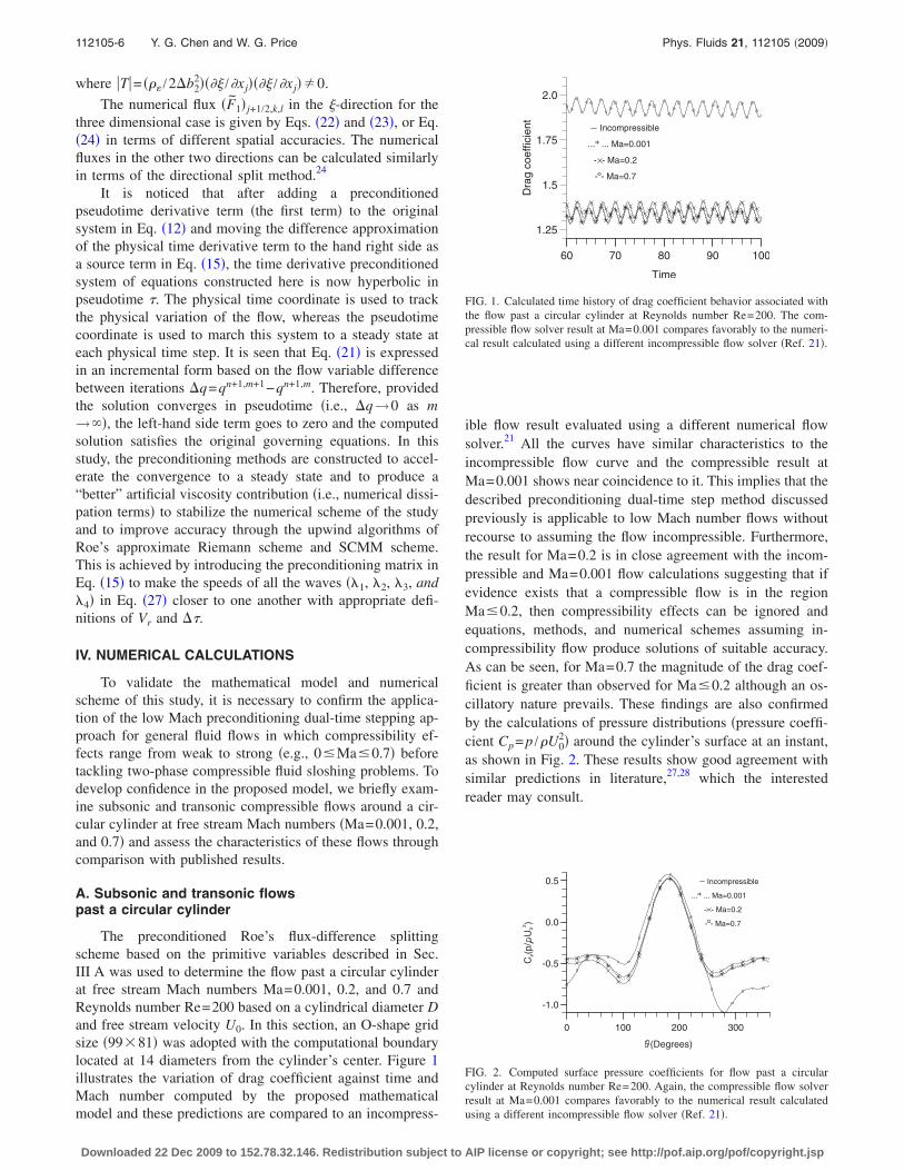
The preconditioned Roe’s flux-difference splittingscheme based on the primitive variables described in Sec.III A was used to determine the flow past a circular cylinderat free stream Mach numbers Ma=0.001, 0.2, and 0.7 andReynolds number Re=200 based on a cylindrical diameter Dand free stream velocity U0. In this section, an O-shape gridsize �9981� was adopted with the computational boundarylocated at 14 diameters from the cylinder’s center. Figure 1illustrates the variation of drag coefficient against time andMach number computed by the proposed mathematicalmodel and these predictions are compared to an incompress-

ible flow result evaluated using a different numerical flowsolver.21 All the curves have similar characteristics to theincompressible flow curve and the compressible result atMa=0.001 shows near coincidence to it. This implies that thedescribed preconditioning dual-time step method discussedpreviously is applicable to low Mach number flows withoutrecourse to assuming the flow incompressible. Furthermore,the result for Ma=0.2 is in close agreement with the incom-pressible and Ma=0.001 flow calculations suggesting that ifevidence exists that a compressible flow is in the regionMa�0.2, then compressibility effects can be ignored andequations, methods, and numerical schemes assuming in-compressibility flow produce solutions of suitable accuracy.As can be seen, for Ma=0.7 the magnitude of the drag coef-ficient is greater than observed for Ma�0.2 although an os-cillatory nature prevails. These findings are also confirmedby the calculations of pressure distributions �pressure coeffi-cient Cp= p /�U0

2� around the cylinder’s surface at an instant,as shown in Fig. 2. These results show good agreement withsimilar predictions in literature,27,28 which the interestedreader may consult.

60 70 80 90 100

Time

1.25

1.5

1.75

2.0

Dra

gco

effic

ient Incompressible

... ... Ma=0.001

- - Ma=0.2

- - Ma=0.7

FIG. 1. Calculated time history of drag coefficient behavior associated withthe flow past a circular cylinder at Reynolds number Re=200. The com-pressible flow solver result at Ma=0.001 compares favorably to the numeri-cal result calculated using a different incompressible flow solver �Ref. 21�.

0 100 200 300

(Degrees)

-1.0

-0.5

0.0

0.5

Cp(

p/U

02 )

Incompressible

... ... Ma=0.001

- - Ma=0.2

- - Ma=0.7

FIG. 2. Computed surface pressure coefficients for flow past a circularcylinder at Reynolds number Re=200. Again, the compressible flow solverresult at Ma=0.001 compares favorably to the numerical result calculatedusing a different incompressible flow solver �Ref. 21�.



B. Validation for liquid sloshing in a moving tank

To make sure that the proposed numerical method devel-oped converges satisfactorily and to illustrate that it providesan acceptable accuracy to simulate impact pressures inducedby sloshing, this section contains selected numerical ex-amples of sloshing in an 80% filled tank subject to harmonictranslational motions. The numerical results derived by theSCMM approach described in Sec. III B are compared toexperimental data. It is noted that the mathematical modeland numerical scheme of study are not restricted to a singlemotion excitation but allow combinations of motions �trans-lations and rotations� in all degrees of freedom as well asirregular excitation inputs.

1. Experimental data

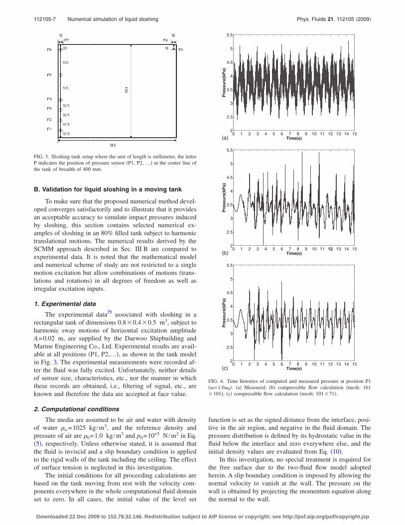
The experimental data29 associated with sloshing in arectangular tank of dimensions 0.80.40.5 m3, subject toharmonic sway motions of horizontal excitation amplitudeA=0.02 m, are supplied by the Daewoo Shipbuilding andMarine Engineering Co., Ltd. Experimental results are avail-able at all positions �P1, P2,…�, as shown in the tank modelin Fig. 3. The experimental measurements were recorded af-ter the fluid was fully excited. Unfortunately, neither detailsof sensor size, characteristics, etc., nor the manner in whichthese records are obtained, i.e., filtering of signal, etc., areknown and therefore the data are accepted at face value.

2. Computational conditions

The media are assumed to be air and water with densityof water �w=1025 kg /m3, and the reference density andpressure of air are �0=1.0 kg /m3 and p0=10+5 N /m2 in Eq.�5�, respectively. Unless otherwise stated, it is assumed thatthe fluid is inviscid and a slip boundary condition is appliedto the rigid walls of the tank including the ceiling. The effectof surface tension is neglected in this investigation.

The initial conditions for all proceeding calculations arebased on the tank moving from rest with the velocity com-ponents everywhere in the whole computational fluid domainset to zero. In all cases, the initial value of the level set

function is set as the signed distance from the interface, posi-tive in the air region, and negative in the fluid domain. Thepressure distribution is defined by its hydrostatic value in thefluid below the interface and zero everywhere else, and theinitial density values are evaluated from Eq. �10�.

In this investigation, no special treatment is required forthe free surface due to the two-fluid flow model adoptedherein. A slip boundary condition is imposed by allowing thenormal velocity to vanish at the wall. The pressure on thewall is obtained by projecting the momentum equation alongthe normal to the wall.

0 1 2 3 4 5 6 7 8 9 10 11 12 13 14 152

2.5

3

3.5

4

4.5

5

5.5

Time(s)

Pre

ssu

re(k

Pa)

(a)

0 1 2 3 4 5 6 7 8 9 10 11 12 13 14 152

2.5

3

3.5

4

4.5

5

5.5

Time(s)

Pre

ssu

re(k

Pa)

(c)

0 1 2 3 4 5 6 7 8 9 10 11 1212 13 14 152

2.5

3

3.5

4

4.5

5

5.5

Time(s)

Pre

ssu

re(k

Pa)

(b)

FIG. 4. Time histories of computed and measured pressure at position P1��=1.0�0�. �a� Measured; �b� compressible flow calculation �mesh: 161101�; �c� compressible flow calculation �mesh: 10171�.

FIG. 3. Sloshing tank setup where the unit of length is millimeter, the letterP indicates the position of pressure sensor �P1, P2, …� at the center line ofthe tank of breadth of 400 mm.



Numerical experiments revealed that the convergence ofthe presented numerical scheme of study is not very sensitiveto the value of the pseudotime step increment �� when of theorder of �510−5�− �110−3� for two-fluid flow computa-tions. For this reason, the value of ��=210−4 was assumedfor all test cases.

3. Resonance frequency excitation

The frequency of excitation considered in this section isset to �=1.0�0=0.945 Hz �where �0 is the natural fre-quency of the rectangular tank� at resonance. Numerical cal-culations were performed using a 161101 uniform mesh

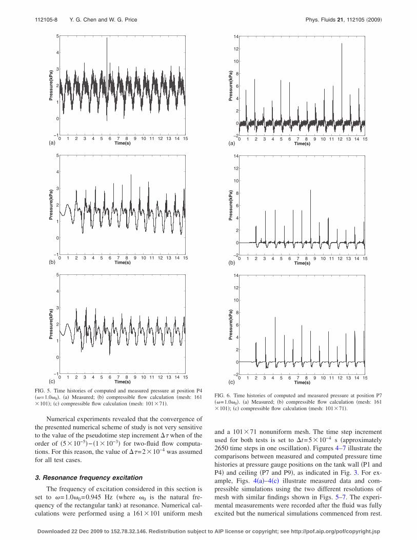
and a 10171 nonuniform mesh. The time step incrementused for both tests is set to �t=510−4 s �approximately2650 time steps in one oscillation�. Figures 4–7 illustrate thecomparisons between measured and computed pressure timehistories at pressure gauge positions on the tank wall �P1 andP4� and ceiling �P7 and P9�, as indicated in Fig. 3. For ex-ample, Figs. 4�a�–4�c� illustrate measured data and com-pressible simulations using the two different resolutions ofmesh with similar findings shown in Figs. 5–7. The experi-mental measurements were recorded after the fluid was fullyexcited but the numerical simulations commenced from rest.

0 1 2 3 4 5 6 7 8 9 10 11 12 13 14 15−1

0

1

2

3

4

5

Time(s)

Pre

ssu

re(k

Pa)

(a)

0 1 2 3 4 5 6 7 8 9 10 11 12 13 14 15−1

0

1

2

3

4

5

Time(s)

Pre

ssu

re(k

Pa)

(b)

0 1 2 3 4 5 6 7 8 9 10 11 12 13 14 15−1

0

1

2

3

4

5

Time(s)

Pre

ssu

re(k

Pa)

(c)


0 1 2 3 4 5 6 7 8 9 10 11 12 13 14 15−2

0

2

4

6

8

10

12

14

Time(s)

Pre

ssu

re(k

Pa)

(a)

0 1 2 3 4 5 6 7 8 9 10 11 12 13 14 15−2

0

2

4

6

8

10

12

14

Time(s)

Pre

ssu

re(k

Pa)

(b)

0 1 2 3 4 5 6 7 8 9 10 11 12 13 14 15−2

0

2

4

6

8

10

12

14

Time(s)

Pre

ssu

re(k

Pa)

(c)




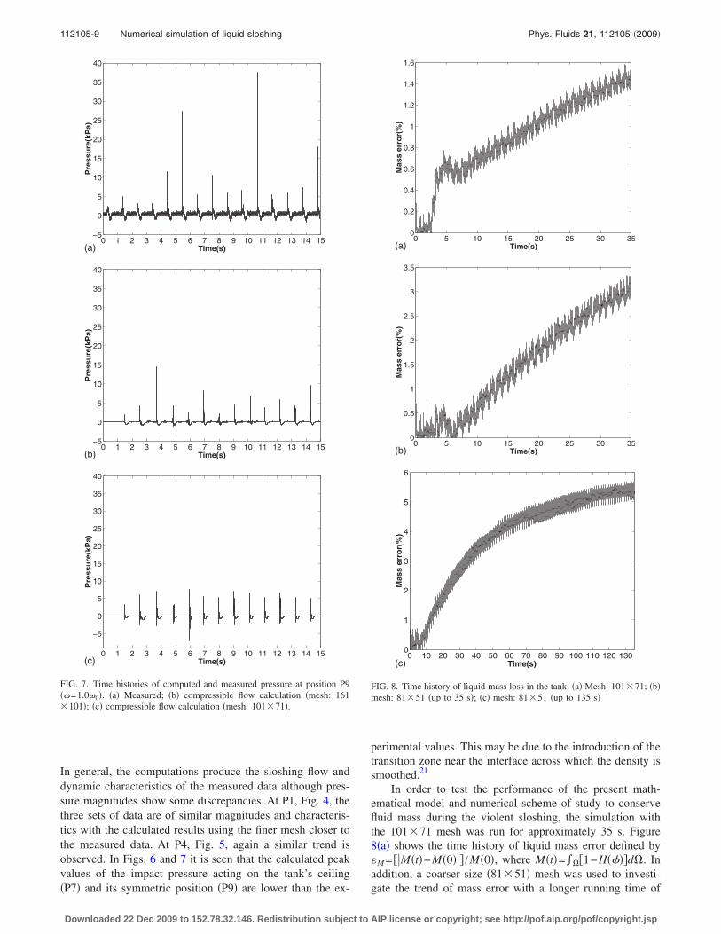
In general, the computations produce the sloshing flow anddynamic characteristics of the measured data although pres-sure magnitudes show some discrepancies. At P1, Fig. 4, thethree sets of data are of similar magnitudes and characteris-tics with the calculated results using the finer mesh closer tothe measured data. At P4, Fig. 5, again a similar trend isobserved. In Figs. 6 and 7 it is seen that the calculated peakvalues of the impact pressure acting on the tank’s ceiling�P7� and its symmetric position �P9� are lower than the ex-

perimental values. This may be due to the introduction of thetransition zone near the interface across which the density issmoothed.21

In order to test the performance of the present math-ematical model and numerical scheme of study to conservefluid mass during the violent sloshing, the simulation withthe 10171 mesh was run for approximately 35 s. Figure8�a� shows the time history of liquid mass error defined by�M = �M�t�−M�0�� /M�0�, where M�t�=��1−H��d�. Inaddition, a coarser size �8151� mesh was used to investi-gate the trend of mass error with a longer running time of

0 1 2 3 4 5 6 7 8 9 10 11 12 13 14 15−5

0

5

10

15

20

25

30

35

40

Time(s)

Pre

ssu

re(k

Pa)

(a)

0 1 2 3 4 5 6 7 8 9 10 11 12 13 14 15−5

0

5

10

15

20

25

30

35

40

Time(s)

Pre

ssu

re(k

Pa)

(b)

0 1 2 3 4 5 6 7 8 9 10 11 12 13 14 15

−5

0

5

10

15

20

25

30

35

40

Time(s)

Pre

ssu

re(k

Pa)

(c)


0 5 10 15 20 25 30 350

0.2

0.4

0.6

0.8

1

1.2

1.4

1.6

Time(s)

Mas

ser

ror(

%)

(a)

0 5 10 15 20 25 30 350

0.5

1

1.5

2

2.5

3

3.5

Time(s)

Mas

ser

ror(

%)

(b)

0 10 20 30 40 50 60 70 80 90 100 110 120 1300

1

2

3

4

5

6

Time(s)

Mas

ser

ror(

%)

(c)

FIG. 8. Time history of liquid mass loss in the tank. �a� Mesh: 10171; �b�mesh: 8151 �up to 35 s�; �c� mesh: 8151 �up to 135 s�



135 s, as shown in Fig. 8�b� �35 s� and Fig. 8�c� �135 s�. It isnoted that the mass error in Fig. 8�c� does not increase lin-early against time, and the growth rate of mass error de-creases with time. The finer mesh results are of the order ofa half smaller, providing evidence that the finer the mesh thesmaller the mass error, but the computational effort greatlyincreases.

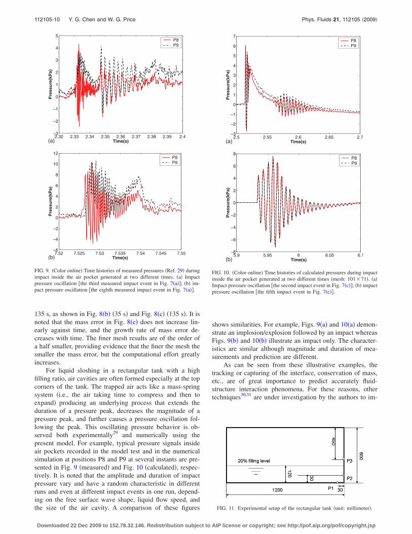
For liquid sloshing in a rectangular tank with a highfilling ratio, air cavities are often formed especially at the topcorners of the tank. The trapped air acts like a mass-springsystem �i.e., the air taking time to compress and then toexpand� producing an underlying process that extends theduration of a pressure peak, decreases the magnitude of apressure peak, and further causes a pressure oscillation fol-lowing the peak. This oscillating pressure behavior is ob-served both experimentally29 and numerically using thepresent model. For example, typical pressure signals insideair pockets recorded in the model test and in the numericalsimulation at positions P8 and P9 at several instants are pre-sented in Fig. 9 �measured� and Fig. 10 �calculated�, respec-tively. It is noted that the amplitude and duration of impactpressure vary and have a random characteristic in differentruns and even at different impact events in one run, depend-ing on the free surface wave shape, liquid flow speed, andthe size of the air cavity. A comparison of these figures

shows similarities. For example, Figs. 9�a� and 10�a� demon-strate an implosion/explosion followed by an impact whereasFigs. 9�b� and 10�b� illustrate an impact only. The character-istics are similar although magnitude and duration of mea-surements and prediction are different.

As can be seen from these illustrative examples, thetracking or capturing of the interface, conservation of mass,etc., are of great importance to predict accurately fluid-structure interaction phenomena. For these reasons, othertechniques30,31 are under investigation by the authors to im-

FIG. 11. Experimental setup of the rectangular tank �unit: millimeter�.

2.32 2.33 2.34 2.35 2.36 2.37 2.38 2.39 2.4−3

−2

−1

0

1

2

3

4

5

Time(s)

Pre

ssu

re(k

Pa)

P8P9

(a)

7.52 7.525 7.53 7.535 7.54 7.545 7.55−6

−4

−2

0

2

4

6

8

10

12

Time(s)

Pre

ssu

re(k

Pa)

P8P9

(b)

FIG. 9. �Color online� Time histories of measured pressures �Ref. 29� duringimpact inside the air pocket generated at two different times. �a� Impactpressure oscillation �the third measured impact event in Fig. 7�a��; �b� im-pact pressure oscillation �the eighth measured impact event in Fig. 7�a��.

2.5 2.55 2.6 2.65 2.7−3

−2

−1

0

1

2

3

4

5

6

7

Time(s)

Pre

ssu

re(k

Pa)

P8P9

(a)

5.9 5.95 6 6.05 6.1−8

−6

−4

−2

0

2

4

6

8

Time(s)

Pre

ssu

re(k

Pa)

P8P9

(b)

FIG. 10. �Color online� Time histories of calculated pressures during impactinside the air pocket generated at two different times �mesh: 10171�. �a�Impact pressure oscillation �the second impact event in Fig. 7�c��; �b� impactpressure oscillation �the fifth impact event in Fig. 7�c��.



prove the proposed numerical scheme of the study that hasshown versatility in evaluating a wide of range of sloshingphenomena.

C. Sloshing induced impact against a vertical wall

The damage to tank walls by waves inside a tank has notbeen fully explained in fluid mechanical terms. High-speedphotography reveals that the plume of water begins its up-ward motion from the water line with great acceleration. Thisrapidly rising motion of the free surface forming a jet wasdescribed by Peregrine32 as flip through. In this section we

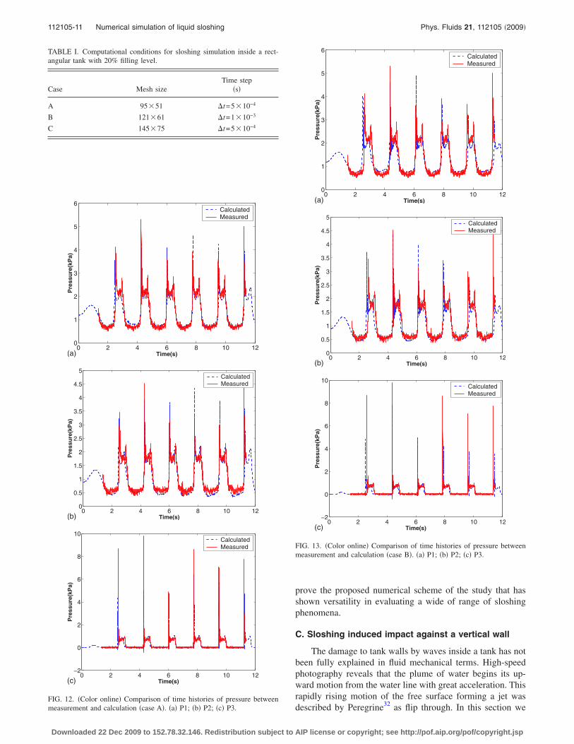
TABLE I. Computational conditions for sloshing simulation inside a rect-angular tank with 20% filling level.

Case Mesh sizeTime step

�s�

A 9551 �t=510−4

B 12161 �t=110−3

C 14575 �t=510−4

0 2 4 6 8 10 120

1

2

3

4

5

6

Time(s)

Pre

ssu

re(k

Pa)

CalculatedMeasured

(a)

0 2 4 6 8 10 120

0.5

1

1.5

2

2.5

3

3.5

4

4.5

5

Time(s)

Pre

ssu

re(k

Pa)

CalculatedMeasured

(b)

0 2 4 6 8 10 12−2

0

2

4

6

8

10

Time(s)

Pre

ssu

re(k

Pa)

CalculatedMeasured

(c)

FIG. 12. �Color online� Comparison of time histories of pressure betweenmeasurement and calculation �case A�. �a� P1; �b� P2; �c� P3.

0 2 4 6 8 10 120

1

2

3

4

5

6

Time(s)

Pre

ssu

re(k

Pa)

CalculatedMeasured

(a)

0 2 4 6 8 10 120

0.5

1

1.5

2

2.5

3

3.5

4

4.5

5

Time(s)

Pre

ssu

re(k

Pa)

CalculatedMeasured

(b)

0 2 4 6 8 10 12−2

0

2

4

6

8

10

Time(s)

Pre

ssu

re(k

Pa)

CalculatedMeasured

(c)

FIG. 13. �Color online� Comparison of time histories of pressure betweenmeasurement and calculation �case B�. �a� P1; �b� P2; �c� P3.



carried out numerical simulation of water sloshing in a rect-angular tank at a low filling level of 20%. The experimentaldata provided by Hinatsu et al.33 are compared to calculateddata derived by the discussed mathematical model herein.The experimental setup is sketched in Fig. 11. The tank issubject to an oscillating sway motion of the form A sin��t�.Here, the amplitude of forced motion is A=60 mm and theexcited frequency is set to �=1.74 s at resonance. In orderto demonstrate the efficiency of the developed method tosimulate the complex impact phenomena, three test cases

were performed to analyze the first impact event. Thecomputational conditions for these three cases are listed inTable I.

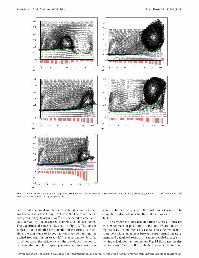
The comparisons of calculated time histories of pressurewith experiment at positions P1, P2, and P3 are shown inFig. 12 �case A� and Fig. 13 �case B�. These figures demon-strate very close agreement between experimental measure-ments and calculated results. In a more detailed analysis in-volving calculations at fixed times, Fig. 14 illustrates the firstimpact event for case B in which a wave is excited and

−0.6 −0.4 −0.2 0 0.2 0.4 0.6−0.1

0

0.1

0.2

0.3

0.4

0.5

0.6

(a)

−0.6 −0.4 −0.2 0 0.2 0.4 0.6−0.1

0

0.1

0.2

0.3

0.4

0.5

0.6

(b)

−0.6 −0.4 −0.2 0 0.2 0.4 0.6 0.8−0.2

−0.1

0

0.1

0.2

0.3

0.4

0.5

0.6

(c)

−0.6 −0.4 −0.2 0 0.2 0.4 0.6−0.1

0

0.1

0.2

0.3

0.4

0.5

0.6

0.7

0.8

(d)

−0.6 −0.4 −0.2 0 0.2 0.4 0.6−0.1

0

0.1

0.2

0.3

0.4

0.5

0.6

(e)

FIG. 14. �Color online� Wave motion snapshots during the first impact event at five different instants of time �case B�. �a� Time=2.21 s; �b� time=2.50 s; �c�time=2.52 s; �d� time=2.60 s; �e� time=2.85 s.



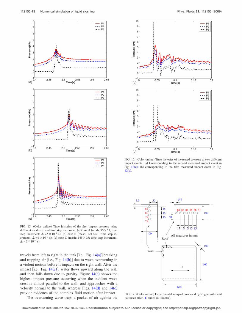
travels from left to right in the tank �i.e., Fig. 14�a�� breakingand trapping air �i.e., Fig. 14�b�� due to wave overturning ina violent motion before it impacts on the right wall. After theimpact �i.e., Fig. 14�c��, water flows upward along the walland then falls down due to gravity. Figure 14�c� shows thehighest impact pressure occurring when the incident wavecrest is almost parallel to the wall, and approaches with avelocity normal to the wall, whereas Figs. 14�d� and 14�e�provide evidence of the complex fluid motion after impact.

The overturning wave traps a pocket of air against the

2.4 2.45 2.5 2.55 2.6 2.65−1

0

1

2

3

4

5

6

7

8

Time(s)

Pre

ssu

re(k

Pa)

P1P2P3

(a)

2.4 2.45 2.5 2.55 2.6 2.65−1

0

1

2

3

4

5

6

7

8

Time(s)

Pre

ssu

re(k

Pa)

P1P2P3

(b)

2.4 2.45 2.5 2.55 2.6 2.65−1

0

1

2

3

4

5

6

7

8

Time(s)

Pre

ssu

re(k

Pa)

P1P2P3

(c)

FIG. 15. �Color online� Time histories of the first impact pressure usingdifferent mesh size and time step increment. �a� Case A �mesh: 9551; timestep increment: �t=510−4 s�; �b� case B �mesh: 12161; time step in-crement: �t=110−3 s�; �c� case C �mesh: 14575; time step increment:�t=510−4 s�.

0 0.05 0.1 0.15 0.2−1

0

1

2

3

4

5

6

7

8

9

10

Time(s)

Pre

ssu

re(k

Pa)

P1P2P3

(a)

0 0.05 0.1 0.15 0.2−1

0

1

2

3

4

5

6

7

8

9

10

Time(s)

Pre

ssu

re(k

Pa)

P1P2P3

(b)

FIG. 16. �Color online� Time histories of measured pressure at two differentimpact events. �a� Corresponding to the second measured impact event inFig. 12�c�; �b� corresponding to the fifth measured impact event in Fig.12�c�.

� � � �

��

50

All measures in mm

T1

Wall

Roof

3.3 50 5.8

100

100

600

600

100

15

15

15

15 15 15 15 15

81

80

79

78

82 83 84 85 86 87

FIG. 17. �Color online� Experimental setup of tank used by Rognebakke andFaltinsen �Ref. 1� �unit: millimeter�.



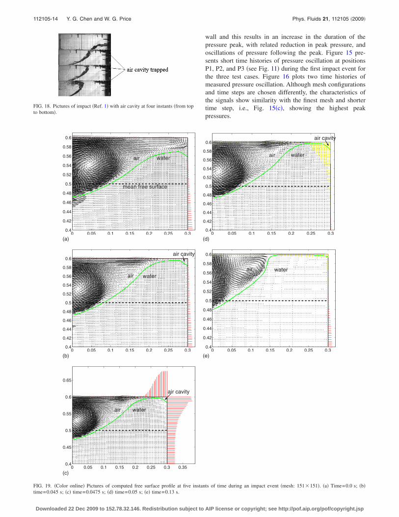
wall and this results in an increase in the duration of thepressure peak, with related reduction in peak pressure, andoscillations of pressure following the peak. Figure 15 pre-sents short time histories of pressure oscillation at positionsP1, P2, and P3 �see Fig. 11� during the first impact event forthe three test cases. Figure 16 plots two time histories ofmeasured pressure oscillation. Although mesh configurationsand time steps are chosen differently, the characteristics ofthe signals show similarity with the finest mesh and shortertime step, i.e., Fig. 15�c�, showing the highest peakpressures.

FIG. 18. Pictures of impact �Ref. 1� with air cavity at four instants �from topto bottom�.

0 0.05 0.1 0.15 0.2 0.25 0.30.4

0.42

0.44

0.46

0.48

0.5

0.52

0.54

0.56

0.58

0.6

air water

mean free surface

(a)

0 0.05 0.1 0.15 0.2 0.25 0.30.4

0.42

0.44

0.46

0.48

0.5

0.52

0.54

0.56

0.58

0.6

air water

air cavity

(b)

0 0.05 0.1 0.15 0.2 0.25 0.3 0.350.4

0.45

0.5

0.55

0.6

0.65

air water

air cavity

(c)

0 0.05 0.1 0.15 0.2 0.25 0.30.4

0.42

0.44

0.46

0.48

0.5

0.52

0.54

0.56

0.58

0.6

air water

air cavity

(d)

0 0.05 0.1 0.15 0.2 0.25 0.30.4

0.42

0.44

0.46

0.48

0.5

0.52

0.54

0.56

0.58

0.6

air water

(e)

FIG. 19. �Color online� Pictures of computed free surface profile at five instants of time during an impact event �mesh: 151151�. �a� Time=0.0 s; �b�time=0.045 s; �c� time=0.0475 s; �d� time=0.05 s; �e� time=0.13 s.



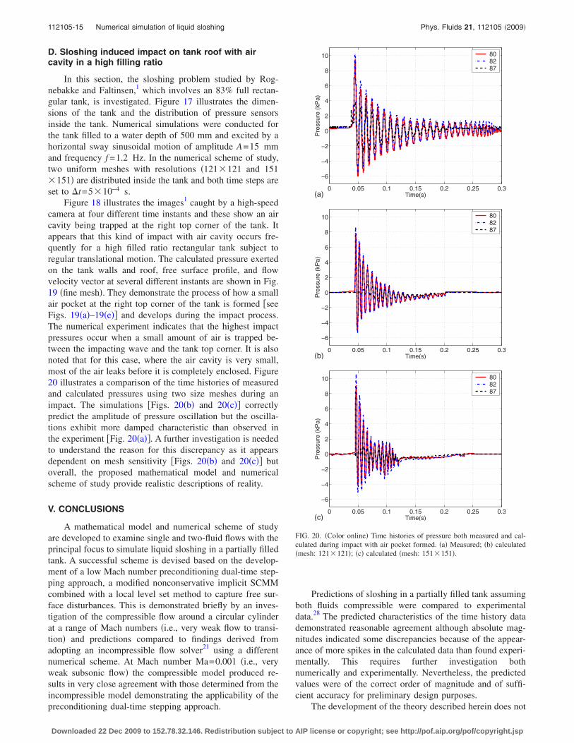
D. Sloshing induced impact on tank roof with aircavity in a high filling ratio

In this section, the sloshing problem studied by Rog-nebakke and Faltinsen,1 which involves an 83% full rectan-gular tank, is investigated. Figure 17 illustrates the dimen-sions of the tank and the distribution of pressure sensorsinside the tank. Numerical simulations were conducted forthe tank filled to a water depth of 500 mm and excited by ahorizontal sway sinusoidal motion of amplitude A=15 mmand frequency f =1.2 Hz. In the numerical scheme of study,two uniform meshes with resolutions �121121 and 151151� are distributed inside the tank and both time steps areset to �t=510−4 s.

Figure 18 illustrates the images1 caught by a high-speedcamera at four different time instants and these show an aircavity being trapped at the right top corner of the tank. Itappears that this kind of impact with air cavity occurs fre-quently for a high filled ratio rectangular tank subject toregular translational motion. The calculated pressure exertedon the tank walls and roof, free surface profile, and flowvelocity vector at several different instants are shown in Fig.19 �fine mesh�. They demonstrate the process of how a smallair pocket at the right top corner of the tank is formed �seeFigs. 19�a�–19�e�� and develops during the impact process.The numerical experiment indicates that the highest impactpressures occur when a small amount of air is trapped be-tween the impacting wave and the tank top corner. It is alsonoted that for this case, where the air cavity is very small,most of the air leaks before it is completely enclosed. Figure20 illustrates a comparison of the time histories of measuredand calculated pressures using two size meshes during animpact. The simulations �Figs. 20�b� and 20�c�� correctlypredict the amplitude of pressure oscillation but the oscilla-tions exhibit more damped characteristic than observed inthe experiment �Fig. 20�a��. A further investigation is neededto understand the reason for this discrepancy as it appearsdependent on mesh sensitivity �Figs. 20�b� and 20�c�� butoverall, the proposed mathematical model and numericalscheme of study provide realistic descriptions of reality.

V. CONCLUSIONS

A mathematical model and numerical scheme of studyare developed to examine single and two-fluid flows with theprincipal focus to simulate liquid sloshing in a partially filledtank. A successful scheme is devised based on the develop-ment of a low Mach number preconditioning dual-time step-ping approach, a modified nonconservative implicit SCMMcombined with a local level set method to capture free sur-face disturbances. This is demonstrated briefly by an inves-tigation of the compressible flow around a circular cylinderat a range of Mach numbers �i.e., very weak flow to transi-tion� and predictions compared to findings derived fromadopting an incompressible flow solver21 using a differentnumerical scheme. At Mach number Ma=0.001 �i.e., veryweak subsonic flow� the compressible model produced re-sults in very close agreement with those determined from theincompressible model demonstrating the applicability of thepreconditioning dual-time stepping approach.

Predictions of sloshing in a partially filled tank assumingboth fluids compressible were compared to experimentaldata.28 The predicted characteristics of the time history datademonstrated reasonable agreement although absolute mag-nitudes indicated some discrepancies because of the appear-ance of more spikes in the calculated data than found experi-mentally. This requires further investigation bothnumerically and experimentally. Nevertheless, the predictedvalues were of the correct order of magnitude and of suffi-cient accuracy for preliminary design purposes.

The development of the theory described herein does not

0 0.05 0.1 0.15 0.2 0.25 0.3

−6

−4

−2

0

2

4

6

8

10

Time(s)

Pre

ssur

e(k

Pa)

808287

(a)

0 0.05 0.1 0.15 0.2 0.25 0.3

−6

−4

−2

0

2

4

6

8

10

Time(s)

Pre

ssur

e(k

Pa)

808287

(b)

0 0.05 0.1 0.15 0.2 0.25 0.3

−6

−4

−2

0

2

4

6

8

10

Time(s)

Pre

ssur

e(k

Pa)

808287

(c)

FIG. 20. �Color online� Time histories of pressure both measured and cal-culated during impact with air pocket formed. �a� Measured; �b� calculated�mesh: 121121�; �c� calculated �mesh: 151151�.



necessitate an a priori assumption of incompressibility sinceit has been shown to adequately replicate this condition fromthe standpoint of compressibility. Furthermore, if and whenstrong compressibility effects occur in the sloshing problem�i.e., entrapped air arising in violent motions�, it is able totake them into account and hence the developed dynamicmathematical model describes such physical phenomena andtheir influences with greater accuracy. This is demonstratedin comparisons of experimental observations1,29,33 and nu-merical predictions.

ACKNOWLEDGMENTS

Y. G. Chen is grateful for the funding of this investiga-tion from Lloyd’s Register University Technology Centre,School of Engineering Sciences. The authors would like toexpress their gratitude to Dr. D. H. Kang and Dr. Y. B. Lee ofthe Daewoo Shipbuilding and Marine Engineering Co., LTD,South Korea in providing the experimental data for the firsttest case,29 Dr. M. Hinatsu of the National Maritime Re-search Institute of Japan for the second test case,33 and Dr. O.Rognebakke for providing the tank geometry and experimen-tal details for the last test case.1 The authors are also gratefulto the referees for their valuable comments and constructivesuggestions which have significantly enhanced the manu-script.

1O. Rognebakke, J. R. Hoff, J. Allers, K. Berget, B. O. Berge, and R. Zhao,“Experimental approaches for determining sloshing loads in LNG tanks,”Transactions – Society of Naval Architects and Marine Engineers�SNAME�, Houston, 2005.

2D. H. Peregrine and L. Thais, “The effect of entrained air in violent waterwave impacts,” J. Fluid Mech. 325, 377 �1996�.

3D. J. Wood, D. H. Peregrine, and T. Bruce, “Wave impact on a wall usingpressure-impulse theory. I: Trapped air,” J. Waterway, Port, Coastal,Ocean Eng. 126, 182 �2000�.

4C. Lugni, M. Brocchini, and O. M. Faltinsen, “Wave impact loads: Therole of the flip-through,” Phys. Fluids 18, 122101 �2006�.

5H. Bijl and P. Wesseling, “A unified method for computing incompressibleand compressible flows in boundary-fitted coordinates,” J. Comput. Phys.141, 153 �1998�.

6H. Guillard and C. Viozat, “On the behaviour of upwind schemes in thelow Mach number limit,” Comput. Fluids 28, 63 �1999�.

7S. Venkateswaran, J. W. Lindau, R. F. Kunz, and C. L. Merkle, “Compu-tation of multiphase mixture flows with compressibility effects,” J. Com-put. Phys. 180, 54 �2002�.

8B. Koren and B. van Leer, “Analysis of preconditioning and multigrid forEuler flows with low-subsonic regions,” Adv. Comput. Math. 4, 127�1995�.

9E. Turkel, “Preconditioning techniques in computational fluid dynamics,”Annu. Rev. Fluid Mech. 31, 385 �1999�.

10W. R. Briley, L. K. Taylor, and D. L. Whitfield, “High-resolution viscousflow simulations at arbitrary Mach number,” J. Comput. Phys. 184, 79�2003�.

11S. A. Pandya, S. Venkateswaran, and T. H. Pulliam, “Implementation of

preconditioned dual-time procedures in OVERFLOW,” AIAA Paper No.2003-0072, 2003.

12S. Karni, “Multicomponent flow calculations by a consistent primitivealgorithm,” J. Comput. Phys. 112, 31 �1994�.

13S. Karni, “Hybrid multifluid algorithms,” SIAM J. Sci. Comput. �USA�17, 1019 �1996�.

14B. Koren, M. R. Lewis, E. H. van Brummelen, and B. van Leer,“Riemann-problem and level set approaches for homentropic two-fluidflow computations,” J. Comput. Phys. 181, 654 �2002�.

15J. P. Cocchi, R. Saurel, and J. C. Loraud, “Treatment of interface problemswith Godunov-type schemes,” J. Comput. Phys. 137, 265 �1997�.

16S. F. Davis, “An interface tracking method for hyperbolic systems of con-servation laws,” Appl. Numer. Math. 10, 447 �1992�.

17D. Igra and K. Takayama, “A high resolution upwind scheme for multi-component flows,” Int. J. Numer. Methods Fluids 38, 985 �2002�.

18R. Abgrall, “How to prevent pressure oscillations in multicomponent flowcalculations: A quasi conservative approach,” J. Comput. Phys. 125, 150�1996�.

19R. P. Fedkiw, T. Aslam, B. Merriman, and S. Osher, “A non-oscillatoryEulerian approach to interfaces in multimaterial flows �the ghost fluidmethod�,” J. Comput. Phys. 152, 457 �1999�.

20S. R. Chakravarthy, D. A. Anderson and M. D. Salas, “The split coeffi-cient matrix method for hyperbolic systems of gas dynamic equations,”AIAA Paper No. 80-0268, 1980.

21Y. G. Chen, K. Djidjeli, and W. G. Price, “Numerical simulation of liquidsloshing phenomena in partially filled containers,” Comput. Fluids 38,830 �2009�.

22M. Sussman, P. Smareka, and S. Osher, “A level set approach for comput-ing solutions to incompressible two-phase flows,” J. Comput. Phys. 114,146 �1994�.

23M. Sussman, E. Fatemi, P. Smereka, and S. Osher, “An improved level setmethod for incompressible two-phase flows,” Comput. Fluids 27, 663�1998�.

24E. F. Toro, Riemann Solvers and Numerical Methods for Fluid Dynamics:A Practical Introduction, 2nd ed. �Springer-Verlag, Berlin, 1999�.

25P. L. Roe, “Approximate Riemann solvers, parameter vectors and differ-ence schemes,” J. Comput. Phys. 43, 357 �1981�.

26C. K. Lombard, J. Bardina, E. Venkatapathy and J. Oliger, “Multi-dimensional formulation of CSSM: An upwind flux difference eigenvectorsplit method for the compressible Navier–Stokes equations,” AIAA PaperNo. 83-1895, 1983.

27P. A. Berthelsen and O. M. Faltinsen, “A local directional ghost cell ap-proach for incompressible viscous flow problems with irregular bound-aries,” J. Comput. Phys. 227, 4354 �2008�.

28R. Ghias, H. Mittal, and H. Dong, “A sharp interface immersed boundarymethod for compressible viscous flows,” J. Comput. Phys. 225, 528�2007�.

29D. H. Kang and Y. B. Lee, “Summary report of sloshing model test forrectangular model,” Daewoo Shipbuilding and Marine Engineering Co.,Ltd., Seoul, Report No. 001, 2005.

30T. Bonometti and J. Magnaudet, “Transition from spherical cap to toroidalbubbles,” Phys. Fluids 18, 052102 �2006�.

31K. M. T. Kleefsman, G. Fekken, A. E. P. Veldman, B. Iwanowski, and B.Buchner, “A volume-of-fluid based simulation method for wave impactproblems,” J. Comput. Phys. 206, 363 �2005�.

32D. H. Peregrine, “Water-wall impact on walls,” Annu. Rev. Fluid Mech.35, 23 �2003�.

33M. Hinatsu, Y. Tsukada, R. Fukasawa, and Y. Tanaka, “Two-phase flowsfor joint research,” Proceedings of the SRI-TUHH Mini Workshop on Nu-merical Simulation of Two-Phase Flows, edited by M. Hinatsu �NationalMaritime Research Institute Japan, Tokyo, 2001�.



http://dx.doi.org/10.1017/S0022112096008166

http://dx.doi.org/10.1061/(ASCE)0733-950X(2000)126:4(182)

http://dx.doi.org/10.1061/(ASCE)0733-950X(2000)126:4(182)

http://dx.doi.org/10.1063/1.2399077

http://dx.doi.org/10.1006/jcph.1998.5914

http://dx.doi.org/10.1016/S0045-7930(98)00017-6



http://dx.doi.org/10.1007/BF02123476

http://dx.doi.org/10.1146/annurev.fluid.31.1.385

http://dx.doi.org/10.1016/S0021-9991(02)00018-9


http://dx.doi.org/10.1137/S106482759528003X



http://dx.doi.org/10.1016/S0168-9274(06)80001-2

http://dx.doi.org/10.1002/fld.251



http://dx.doi.org/10.1016/j.compfluid.2008.09.003


http://dx.doi.org/10.1016/S0045-7930(97)00053-4

http://dx.doi.org/10.1016/0021-9991(81)90128-5

http://dx.doi.org/10.1016/j.jcp.2007.12.022


http://dx.doi.org/10.1063/1.2196451


http://dx.doi.org/10.1146/annurev.fluid.35.101101.161153

numerical simulation of liquid sloshing in a partially ﬁlled...

Documents