Scho

olof

Mat

hem

atic

sU

nive

rsit

yof

Nai

robi

ISSN: 2410-1397

Master Project in Applied Mathematics

Numerical Solution for Hydromagnetic Steady Flow ofLiquid Between Two Parallel Plates Under Applied PressureGradient When Upper Plate Is Moving With ConstantVelocity Under the In�uence of Inclined Magnetic Field

Research Report in Mathematics, Number 33, 2019

DAVID KARANJA KAGAI June 2019

Submi�ed to the School of Mathematics in partial fulfilment for a degree in Master of Science in Applied Mathematics

Master Project in Applied Mathematics University of NairobiJune 2019

Numerical Solution for Hydromagnetic Steady Flow ofLiquid Between Two Parallel Plates Under AppliedPressure Gradient When Upper Plate Is Moving WithConstant Velocity Under the In�uence of InclinedMagnetic FieldResearch Report in Mathematics, Number 33, 2019

DAVID KARANJA KAGAI

School of MathematicsCollege of Biological and Physical sciencesChiromo, o� Riverside Drive30197-00100 Nairobi, Kenya

Master ThesisSubmi�ed to the School of Mathematics in partial fulfilment for a degree in Master of Science in Applied Mathematics

Submi�ed to: The Graduate School, University of Nairobi, Kenya

ii

Abstract

The current paper explores the steady laminar �ow of viscous in compressible �uid between

two parallel in�nite plates when a pressure gradient which is constant is imposed on the

system and the top plate is also stimulating with continual velocity and lower plate is held

stationery under the in�uence of magnetic �eld.

The guiding partial di�erential equation is changed into ordinary di�erential equation

and the solved numerically using central di�erence method and analytically using laplace

transformation method done by Singh,2014.

The e�ect of the arising important parameter on �ow characteristics has been discussed

through tables A comparative study has been taken into account between existing results

and present work and it has been found to be in excellent harmony

The numerical expression for �uid velocity at a di�erent inclination has been shown on

the table and graph which shows that the increase of inclination of magnetic �eld there is

a decrease in velocity pro�le.

Master Thesis in Mathematics at the University of Nairobi, Kenya.ISSN 2410-1397: Research Report in Mathematics©David K Kagai, 2019DISTRIBUTOR: School of Mathematics, University of Nairobi, Kenya

iv

Declaration and Approval

I the undersigned declare that this dissertation is my original work and to the best of my

knowledge, it has not been submitted in support of an award of a degree in any other

university or institution of learning.

Signature Date

DAVID KARANJA KAGAI

Reg No. I56/8572/2017

In my capacity as a supervisor of the candidate’s dissertation, I certify that this dissertation

has my approval for submission.

Signature Date

Prof C.B.Singh

School of Mathematics,

University of Nairobi,

Box 30197, 00100 Nairobi, Kenya.

E-mail: cbsingh47@yahoo.com

vii

Dedication

This project is dedicated to my parents: Julius Kagai and Grace Mukami And lastly to my

entire family

viii

Contents

Abstract ................................................................................................................................ ii

Declaration and Approval..................................................................................................... iv

Dedication .......................................................................................................................... vii

Acknowledgments ............................................................................................................... ix

1 Introduction ................................................................................................................... 1

1.1 Recent research .................................................................................................................. 2

2 Chapter 2 ....................................................................................................................... 4

2.1 Preliminaries ...................................................................................................................... 42.2 Definition ........................................................................................................................... 4

2.2.1 Properties of fluid ....................................................................................................... 42.2.2 Types of force acting on a moving fluid ........................................................................... 52.2.3 Classification of fluid flow phenomena ........................................................................... 6

2.3 DIMENSION ANALYSIS ...................................................................................................... 72.4 NON DIMENSIONAL NUMBERS IN FLUID DYNAMICS...................................................... 92.5 Numerical Method ........................................................................................................... 13

2.5.1 Single step ............................................................................................................... 142.5.2 Multiple step ........................................................................................................... 14

2.6 Boundary-value problem(B.V.P) ......................................................................................... 152.6.1 Second Order B.v.p ................................................................................................... 15

2.7 EQUATION OF CONTINUITY IN CARTESIAN COORDINATES .......................................... 192.8 EQUATION OF MOTION .................................................................................................. 23

3 Defining the problem.................................................................................................... 27

3.1 THE GOVERNING EQUATION.......................................................................................... 273.1.1 NON DIMENSIONLIZING .......................................................................................... 30

4 DISCUSSION OF RESULTS AND APPLICATIONS ........................................................... 50

Bibliography....................................................................................................................... 51

ix

Acknowledgments

To start with, I thank the almighty God for taking me this far,conferring me with strength,ability and opportunity to undertake this research study ,Without His blessing i wouldn’thave achieved this .

Toward my journey of this degree i met a pillar of support in my guide Prof C.B.Singh,whogave endless guidance and encouragement throughout the entire course of this work andfor ensuring i stay in line without deviating from heart of my research . Without hisadvice this research would not have succeeded and i shall forever be grateful to him forhis backing.

I acknowledge my sincere recognition to the University of Nairobi through the School ofMathematics for the opportunity awarded to me to pursue this studies,without which, Icould not have made to this far.

I take pleasure in recognizing the University of Nairobi lectures ;Dr.Charles Nyandwi ,Prof.Ogana ,Prof Pokhariyal Ganesh ,Dr were for taking me through this course on variouscourse unit

I have great pleasure in endorsing my obligation to my classmates at university ofNairobi;Collins Kiragu ,Sheila Kariaga,Pre�y Cynthia Nyarara ,Lewis Kivuva,Flora Mwikali,Julius Ngugi, Felix Murithi and Eric Ombasa in making sure that the fire kept burning andbeing available anytime i needed motivation and propelling me on this research . Theirgroundwork and dependable ideas have made great contribution in the entire thesis.

To my family members,I take this chance to express the deep gratitude from the bo�om ofmy heart to my beloved parents,grandparents and my sibling for their love and continuoussupport both spiritually and materially

David Karanja Kagai

Nairobi, 2019.

x

1

1 Introduction

The outline of the thesis is as follows:Magneto hydrodynamics (MHD) is a very long word for a very old principle ,the sameprinciple that derive all of of our electric motors and electric generators .E�ectively whena charge particle moves it is asssociated with electric field and by convention we use theright hand rule which state that "to find the direction of the magnetic force on a positivemoving charge,the thumb of the fingers in the direction of b and the force F is directedperpendicular to the right hand palm". magnetic field can induce current in a movingconductive fluid such as plasma,ionized gases liquid metal.

Magneto hydrodynamics (MHD) is as a result of interaction of two branches namelyelectromagnetic theory and fluid dynamic. Assuming that steady flow condition has beena�ained,consider an electrically conducting fluid having a velocity vector V , at right angleto this we apply a magnetic field B .As a result of interaction of the two fields,electricallyfield denoted by E is induced at right angle to both V and B this electrically field is givenby E = V × B.if we assume that the fluid is isotropic we can denote its electrical conductivity by thescalar quantity σ . By Ohms law,the density of the current J induced in the conductingfluid is given by J=α E , i.e., for stationary condition. Simultaneously occurring with theinduced current is the induced electromotive force F=J × B Sin α ,

where α is an angle of inclination of magnetic field with the horizontal.

2

"A familiar model which is normally studied in this thesis consists of an infinitely longchannel of constant cross - section with a uniform static magnetic field applied transverseto the axis of the channel. The walls of channel are either insulators, conductors or acombination of insulators and conductors depending on the intended application. Forexample, in the MHD generator and pump, the channel cross-section is normally circularwith conducting walls"(Singh, 1993).

1.1 Recent research

Serclif (1956) has studied the steady motion of electrically conducting fluid in pipes undertransverse magnetic field.

Drake (1965) has considered the flow in a channel due to periodic pressure gradient andsolved by the method of separation of variables.

Singh and Ram(1977) considered the laminar flow of an electrically conducting fluidthrough a channel in the presence of a transverse magnetic field under the influence ofa periodic pressure gradient and solved it by Laplace transform. Ram et al. (1984) haveconsidered Hall e�ects on heat and mass transfer flow through porous medium.

Simonura (1991) considered magnetohydrodynamic turbulent channel flow under a uni-form transverse magnetic field.

Kazuyuki (1992) discussed inertia e�ects in two dimensional MHD channel flow.

Pop and Watanabe (1995) considered the Hall e�ects on boundary layer flow over a con-tinuous moving flat plate.

Ram(1995)discussed e�ects of Hall and ion slip currents on free convective heat generatingflow in a rotating fluid.

Singh(1998)considered unsteady magnetohydrodynamic flow of liquid through a channelunder variable pressure gradient and solved it by method of Laplace transform.

Singh (2000)considered unsteady flow of liquid through a channel with pressure gradientchanging exponentially under the influence of inclined magnetic field and solved it by

3

method of Laplace transform.

Singh(2014) has considered Hydro-magnetic Steady Flow of Liquid Between Two ParallelInfinite Plates Under Applied Pressure Gradient when Upper Plate is Moving with ConstantVelocity Under the Influence of Inclined Magnetic Field and solved it Laplace transformmethod.

4

2 Chapter 2

2.1 Preliminaries

In this section, we will discuss properties of fluid,classification of fluid flow phenom-ena,dimensional analysis.

2.2 Definition

Fluid :A fluid can be defined as any substance that deform continuously when subjectedto a shear stress

2.2.1 Properties of fluid

viscosity

This is a property of fluid by ideal of which a fluid will o�er resistance to shear stress

Newtonian law of viscosity

This is just a fluid property by virtue of which a fluid o�er resistance.

Non-Newtonian �uid

This are type of fluid that fails to follow newtonians viscosity law(i.e the fluid do not o�erany resistance )*viscocity will change subjected to force either on more liquid or solid.

Pressure

This is the Normal force exerted by a fluid per unit area

5

Density

This is the quantity of ma�er contained in a unit volume of a substance

Speci�c Weight

It is weight per unit volume

Speci�c gravity

This is the ratio of its weight to that of an equal volume of water at a specific temperatureusually at 4◦C

2.2.2 Types of force acting on a moving fluid

Inertia force

Inertia force is equal to the mass and acceleration of the moving fluid

Fi =ρAV 2

Elastic force

Elastic force can be defined as the product of elastic stress and area of the flow

Fe= KA =Area x Elastic stress

Viscous force

Viscous force can be said to be equal to the shear stress as a result of viscosity and surfacearea of the fluid flow.

6

Fv =τdudy A = µ

Ud A

Pressure force

This is as a result of product of pressure intensity and flow area Fp = pA

Gravity force

Product of acceleration and gravitation force is said to be the gravity forceFg=ρALg

Surface tension force

Surface tension is the product of of surface tension and the length of the surface of theflowing fluidFs=σd

2.2.3 Classification of fluid flow phenomena

Steady and unsteady �ow

"Steady flow can be defined as A flow whose flow state expressed by velocity, pressure,density, etc., at any position, does not vary with time,while unsteady flow is a flow whoseflow state does vary or change with time is called an unsteady flow"(Nakayama,1998).

Lamina �ow and turbulent �ow

This can be described as which the flow follows a smooth path and also the path do notinterfere with other, we refer this flow as lamina flow(particle flow along well definedstream line) while the flow which the flow is irregular is referred to as the turbulent flow

7

Uniform �ow and Non uniform �ow

Uniform flow can be defined as the flow in which velocity at any point does not changewith respect to space while Non uniform flow is the flow which velocity changes at anygiven time with respect to time

Compressible Flows and In-compressible

Compressible flow is the flow which density vary at some point (density is not constant)incompressible flow the density is said to be constant at any point

Rotational �ow and irrotational �ow

Rotational flow is defined as flow in which fluid particle rotate on their own axis whileflowing along a streamline

Irrotational flow is defined as flow in which fluid particle do not rotate on their own axiswhile flowing along a streamline or a path

2.3 DIMENSION ANALYSIS

Buckingham pi Theorem

Non-dimensional parameters are as a result of dimensional analysis for the experimentaldata of unknow flow problem.This non -dimensional parameter are re�ered to as pi termsand may be be grouped and expressed in functional forms this was illustrated by EdgarBuckingham (1867-1940)

Buckingham pi theorem, states that if an equation involving k variables is dimensionallyhomogeneous, then it can be reduced to a relationship among (k -r ) independent dimen-sionless products, where r is the minimum number of reference dimensions required todescribe the variable. For a physical system, involving k variables, the functional relationof variables can be wri�en mathematically as, y = f (X1 , X2,X3 .........., Xk )

π1 =ϕ(π2,π2,πk−r)

8

How to determine pi terms

Step 1

Write down all the variables involved in the problem defined and ensure they are allindependent in nature to minimize variables needed to describe the structure

Step 2 Each variables should be expressed in terms of the basic dimension (M,L,TORF,L,T )

Step 3

"Apply the buckingham pi theorem which claims that the number of pi terms is equal to(k-r),where k is number of variables and r is the number of reference dimension requiredto describe the variables" (Watanabe, 1995)

Step 4 Select the variables which can be joined to lead to pi terms (ie duplicating variablesequals the number of reference dimension)

Step 5 "The pi terms are formed by multiplying one of the non-repeating variables bythe product of the repeating variables each raised to an exponent that will make thecombination dimensionless.Usually denoted as xi,xa

1,xbi ,xc

3 the exponents ab c , and aredetermined so that the combination is dimensionless"(Watanabe, 1995).

step 6 For the remaining non -repeating variables ,repeat step 5

step 7

Substitute the common dimension (M,L,T ) of the terms which are not constant into thepi terms to ensure that all the pi terms are dimensionless

9

2.4 NON DIMENSIONAL NUMBERS IN FLUID DYNAMICS

DYNAMICALLY SIMILAR Two system are claimed to be dynamically similar when theseveral force acting on corresponding fluid element have the same ratio to one another inboth system ,so that the path followed by the corresponding elements in the two systemwill be geometrically similar

GEOMETRICALLY SIMILAR Two system are dynamically similar when the ratio of corre-sponding length in the two system is constant so that one is scale model of the other

Let L be the characteristic length in the system under consideration ,for example thediameter of a pipe ,and t a typical time ,then the mass of an element is proportion to ρ l3

and its acceleartion to Lt2 ,so that

inertial force α mass x acceleration

inertial force αρl3 x lt2

inertial force αρl2 x ( lt )

2

since vαlt

inertial force αρl2v2

REYNOLDS NUMBER,Re

Reynolds number is defined as the ratio of inertia force to that of the viscous force.Thisnumber is used for indication of whether a fluid flow through a body is turbulentThus for viscous resistance the requirement for dynamically similarity in the two systemis equality of Reynolds number

10

PROOF

If the motion is controlled by viscous resistance ,the flow in the two system will be dy-namically similar if both the ratio inertia force and the viscous force are similar

Viscous force α viscous shear stress x area

Viscous force α µ x velocity gradient x l2

but velocity gradient αvl

Viscous force α µvl x l2

Viscous force α µ v x l2

inertia f orceviscous f orce α

ρvl2

µvl αρvlµ

FROUDE NUMBER,Fr

This dimensionless number is used for indication of the e�ect or the gravity influence ona fluid two system are dynamically similar for wave resistance if the froude number is thesame for both system

proof

For wave resistance the resisting force is due to gravity

Gravity force = masss x gravitational acceleration

Gravity force α ρl3 x g

inertia f orcegravity f orce α

ρl2v2

ρl3g

11

inertia f orcegravity f orce α

v√lg

which is froude number

MACH NUMBER,Ma

For elastic compression of a fluid the elastic force is dependent on the bulk module k ofthe fluidThe Bulk modulus can be defined as the elastic properties of a liquid or solid when underpressure on both surfaceThe compressibility e�ects dynamical similarity is a�ained when the mach number is thesame in both system

proof

Elastic force α K l2

Thus

inertiasur f acetension f orce α

ρv2l2

kl2

This is the mach number

WEBER NUMBER ,We

This is a dimensionless number that is used for analyzing the fluid flow in case an interfacetakes place between two di�erent fluids. Weber number is used as the ratio betweenboth the inertia force and the surface tension,and is used to indicate whether the sur-face tension is dominant for surface tension e�ect if T is the surface tension per unit length ,

12

surface tension force αTl

Andinertia f orce

sur f acetension αρv2l2

T l

HARTMANN NUMBER ,Ha

This is a dimension less number that is used to indicate the ratio between the magneticviscosity and the ordinary viscosity in the flow (This is the ratio of magnetic force to theviscous force)

Its ussually denoted as

Ha= BL√

σ

µ

B is the magnetic field

L is the characteristic length scale

σ is the electrical conductivity

µ is the dynamic viscosity

Hartman number is usually encountered in fluid flow through a magnetic fields

13

2.5 Numerical Method

Central Di�erence Method

To develop a scheme for solving an equation such as

dydt

= f (t,y);y(t0) = y0

For this equation to be solved numerically, we will have to make some assumption thati) The solution existii)The solution is unique

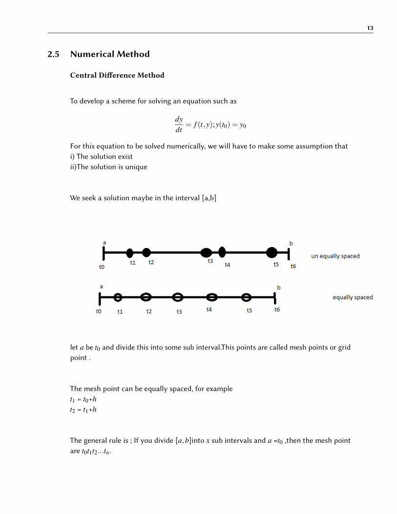
We seek a solution maybe in the interval [a,b]

let a be t0 and divide this into some sub interval.This points are called mesh points or gridpoint .

The mesh point can be equally spaced, for examplet1 = t0+ht2 = t1+h

The general rule is ; If you divide [a,b]into x sub intervals and a =t0 ,then the mesh pointare t0t1t2...tn.

14

Suppose we evaluate this equation at tn

(dydt

)tn = f (tn,yn)

Approximate this and express derivatives in terms of t , tn , tn−1 . This will help to get y(tn), y(tn−1)............

2.5.1 Single step

Single step :This involves using a one step backward or expressing the value at its imme-diate points.

2.5.2 Multiple step

Multiple step It involves expressing the value at its immediate multiple points Lets considera typical mesh points tn

Approximating the derivative at tn, we consider a function

y(t +h) = y(t)+hy′(t)

1!+

h2y′′(t)2!

+h3y′′′(t)

3!..

y(t−h) = y(t)− hy′(t)1!

+h2y′′(t)

2!− h3y′′′(t)

3!...

15

There are di�erents way of approximating

i)Forward di�erence approximation

y′(t) =y(t +h)− y(t)

h− h

2!y′′(t)− h2

3!y′′′(t)

ii)Backward Di�erence Approximation.

y′(t) =y(t)− y(t−h)

h+

h2!

y′′(t)− h2

3!y′′′(t)+ ...

And use

y′(t) =y(tn)− y(tn−1)

h

iii)Central di�erence approximation

Subtracting the first equation from the second equation we get

y′(t) =y(t +h)− y(t−h)

2h+

h2

3!

y′(t) =y(t +h)− y(t−h)

2h+0h2

Note :Numerical equation reduces a di�erential equation to a di�erence equation.

2.6 Boundary-value problem(B.V.P)

This are the values of the di�erential equation solved subject to specified condition at twoor more points.

2.6.1 Second Order B.v.p

1)Boundary condition of first kind y(a) = γ1 , y(b) = γ2

16

2)Boundary condition of the second kind y′(a) = γ1 , y′(b) = γ2

3)Boundary condition of the 3rd kind α1(a)+α2(b)

Steps for solving a BVP

Given an equation

y′′(x)+q1(x)y′(x)+q0y(x) = r(x)

Which is solved in subject

to y(a) = γ1 , y(b) = γ2

Divide [a,b] into N equal sub intervals each of width h

Using central di�erence

yn+1−2yn + yn−1

h2 +q1n

(yn+1− yn−1

2h

)+q0nyn = γn

Multiply bot side by h2.

yn+1−2yn + yn−1 +hq1n

(yn+1− yn−1

2

)+h2q0nyn = h2

γn

Arranging the terms together

(1− 12

hq1h)yn−1 +(h2q01−2)yn +(1+hq1n

2)yn+1 = h2rn

17

Appling the boundary conditions and substituting accordingly we have n=1

(h2q01−2)y1 +(1+12

hq11)y2

n=2(1− 1

2hq1,2)y1 +(h2q02−2)y2 +(1+

12

hq1,2)y30 = h2r2

n=3(1− 1

2hq1,3)y1 +(h2q0,3−2)y3 +(1+

12

hq1,3)y40 = h2r3

n=N-2

0+(1− 12

hq1,N−2)yN−3 +(h2q0N−2−2)yN−2 +(1+12

hq1,N−2)yN−1 = h2rN−2

n=N-1

0+(1− 12

hq1,N−1)yN−2 +(h2q0,N−1−2)yN−1 = h2rN−1− (1+12

hq1,N−1γ2

let

bi=(h2q0,1−2) ;i=2 ,3.....N-1

ci=1+12

hq1i.;i=1,2....N-1

di=h2r1-(1-12

hq11)γ1 ;i=2,3...

ai=1− 12

hq1i ;i=2,3....

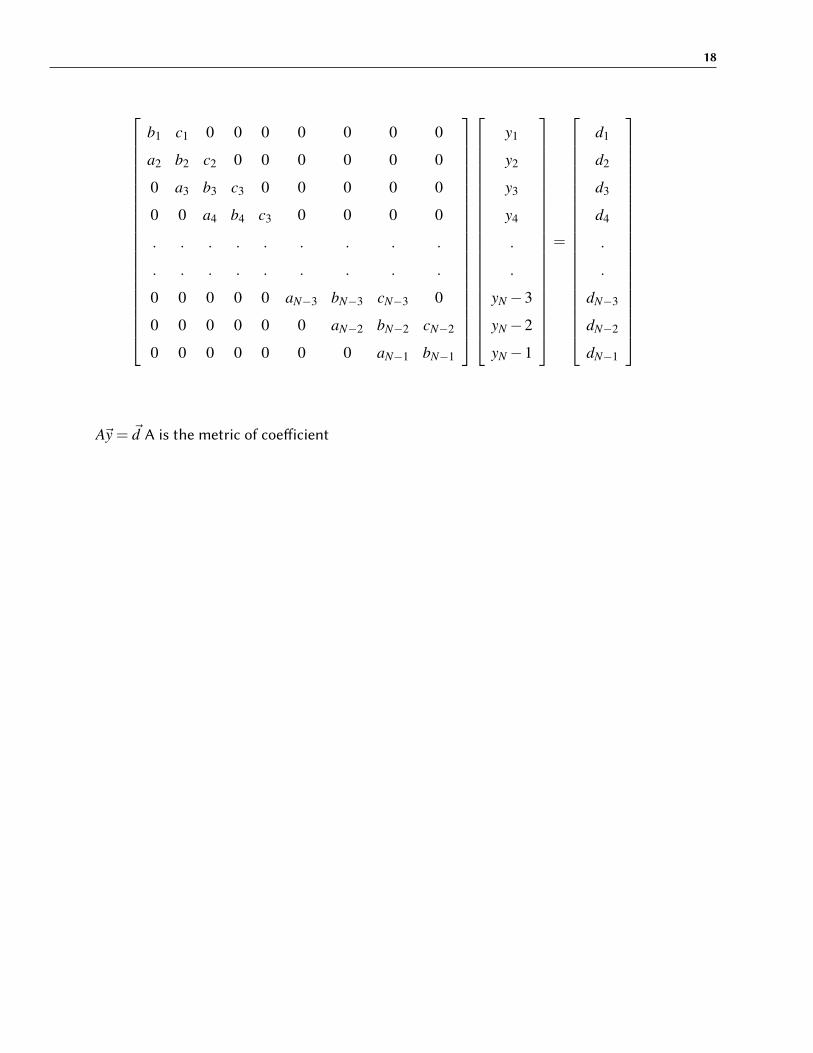
18

b1 c1 0 0 0 0 0 0 0

a2 b2 c2 0 0 0 0 0 0

0 a3 b3 c3 0 0 0 0 0

0 0 a4 b4 c3 0 0 0 0

. . . . . . . . .

. . . . . . . . .

0 0 0 0 0 aN−3 bN−3 cN−3 0

0 0 0 0 0 0 aN−2 bN−2 cN−2

0 0 0 0 0 0 0 aN−1 bN−1

y1

y2

y3

y4

.

.

yN−3

yN−2

yN−1

=

d1

d2

d3

d4

.

.

dN−3

dN−2

dN−1

A~y = ~d A is the metric of coe�icient

19

2.7 EQUATION OF CONTINUITY IN CARTESIAN COORDINATES

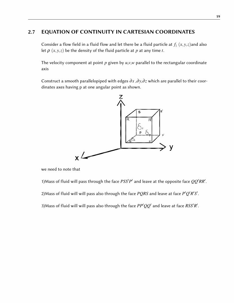
Consider a flow field in a fluid flow and let there be a fluid particle at fz (x,y,z)and alsolet ρ (x,y,z) be the density of the fluid particle at p at any time t .

The velocity component at point p given by u,v,w parallel to the rectangular coordinateaxis

Construct a smooth parallelopiped with edges ∂x ,∂y,∂ z which are parallel to their coor-dinates axes having p at one angular point as shown.

we need to note that

1)Mass of fluid will pass through the face PSS′P′ and leave at the opposite face QQ′RR′.

2)Mass of fluid will will pass also through the face PQRS and leave at face P′Q′R′S′.

3)Mass of fluid will will pass also through the face PP′QQ′ and leave at face RSS′R′.

20

The whole amount of mass of fluid which passes in through the face pssp′

Total mass in =(ρ ∂y ∂ z)

= f (x,y,z)dxdz

Mass of fluid which passes out via the opposite face QRR′Q′

Total mass out =f(x+δx,y,z) per unit time

=f(x,y,z)+ δx ∂ f∂x (x,y,z)

Expanding this using Taylor series expansion The increase of mass of fluid per unit timethrough the face is

=f(x,y,z)-[f(x,y,z)+ δx ∂ f∂x (x,y,z)]

=-δx ∂ f∂x (x,y,z)]

=- ∂

∂x (ρu) ∂x ∂y ∂ z

Similarly the total increase in mass through the face PQRS and P’Q’R’S’

=– ∂

∂x (ρV) ∂x ∂y ∂ z

The amount of mass per unit time with element from the flow via the face PP’QQ’ andRSS’R’ Will be given by

21

=- ∂

∂x (ρw) ∂x ∂y ∂ z

Applying the law of conservation of mass which state

"The rate of increase of the mass of fluid within an element must be equal to therate of mass through into the element"

∂

∂ tρ∂x∂y∂ z =−

(∂

∂x(ρu)+

∂

∂x(ρv)

∂

∂x(ρw)

)∂x∂y∂ z

=∂

∂ tρ =−

(∂

∂x(ρu)+

∂

∂x(ρv)

∂

∂x(ρw)

)

=∂

∂ tρ +

(∂

∂x(ρu)+

∂

∂x(ρv)

∂

∂x(ρw)

)= 0

Which is equation of continuity in Cartesian coordinates system which may be given as

∂

∂ t ρ +ρ∂u∂x +ρ

∂v∂y+ρ

∂w∂ z + u ∂

∂xρ+v ∂

∂yρ+w ∂

∂ zρ=0

=

(∂

∂ t+u

∂

∂xv

∂

∂y+w

∂

∂ z

)ρ +ρ

(∂u∂x

+∂v∂y

+∂w∂ z

)

Then by the definition of of material derivative given by

DDx

=

(∂

∂ t+u

∂

∂xv

∂

∂y+w

∂

∂ z

)

=DDx

ρ +ρ

(∂u∂x

+∂v∂y

+∂w∂ z

)

Taking the fluid to be in compressible the density must be constant (ie ρ =constant)Then the above equation reduces to

∂u∂x

+∂v∂y

+∂w∂ z

22

which refers to the equation of continuity for an incompressible fluid in cartesian

Dealing with two dimensional we have

∂u∂x + ∂v

∂y =0

23

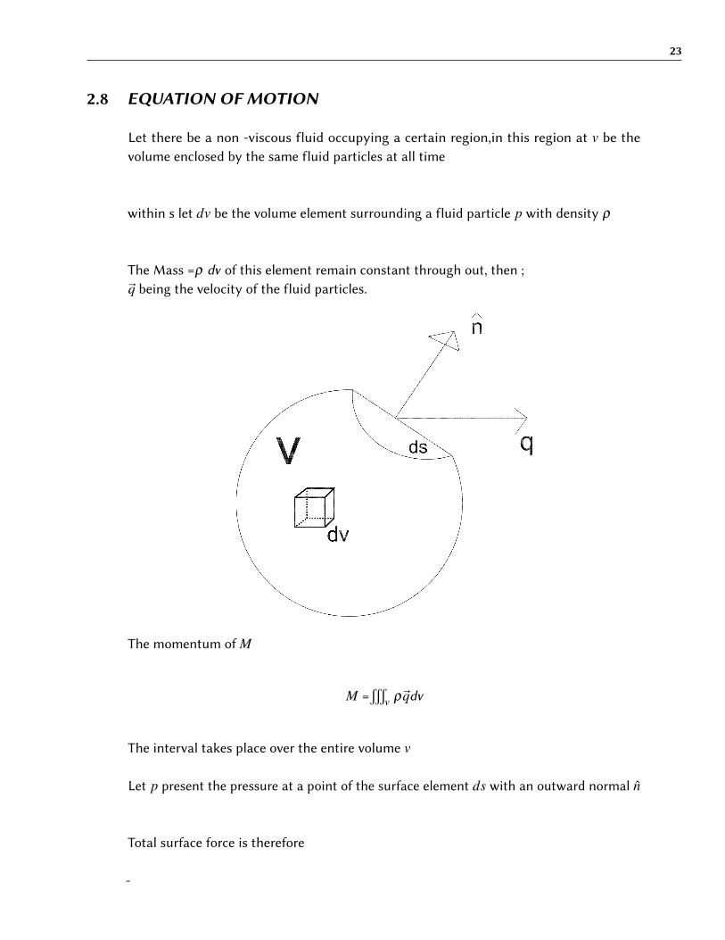
2.8 EQUATION OF MOTION

Let there be a non -viscous fluid occupying a certain region,in this region at v be thevolume enclosed by the same fluid particles at all time

within s let dv be the volume element surrounding a fluid particle p with density ρ

The Mass =ρ dv of this element remain constant through out, then ;~q being the velocity of the fluid particles.

The momentum of M

M =t

v ρ~qdv

The interval takes place over the entire volume v

Let p present the pressure at a point of the surface element ds with an outward normal n

Total surface force is therefore

-

24

ss pn ds = -

tv ∇pdv by Gauss formular

~F represents the external force per unit mass acting on the fluid so that the total forceacting on the fluid within surface s at any time t is

tv~Fρdv

The total force acting on volume v is

tv~Fρdv-

tv ∇pdv

According to the newton second law ,"the rate of change of linear momentum is equal tothe total acting on the mass fluid "

DmDt =

tv [ρ

~F−∇p]dv

=t

vDqDt ρ dv +

tv ~q

DDt (ρdv

=t

v[ρ~F−∇ρ]dv

tv

DqDt ρdv=

tv[ρ

~F−∇ρ]dv

Note DDt (ρdv)=0

since ρdv is constant

The volume V is taken as an arbitrary volume of the fluid in the area considered

DqDt =~F-X ∇p

ρ

25

which is the euler equation

But DqDt =∂~q

∂ t +(q ·∇)~q

Therefore the euler equation is expressed as

∂~q∂ t +(q ·∇)~q=~F - 1

ρ∇p

Applying the vector identity

∇(~A ·~B)=(~B·)~A)+(~A ·∇)~B+~B× (∇×~A)+~A× (∇×~B)

From this we can show that euler equation can be wri�en in the form

∂~q∂ t + ∇

~q2

2 -~q× curl~q=~F- 1rho∇p

∇[~q ·~q]=(~q ·∇)~q)+(~q ·∇)~q)+~q× (∇×~q)+~q× (∇×~q)

such that

∇(q2)=2(~q ·∇)~q) +2~q× (∇×~q)

(~q∇)~q =∇(~q2

2 - q×(∇×~q)

using this we have

∂q∂ t +∇q2

2 -~q × curl~q= F- 1ρ

∇p

Corollary if~q= ui+v j+wk

26

~F=xi+y j+zki

Then the equation of motion takes the form

DDt [ui+ v j+wk]=(xi+ y j+ zk)- 1

ρ(i∂ p

∂x + j ∂ p∂y +k ∂ p

∂ z )

equating the coe�icient of (i , j,k)

DuDt = X- 1

ρ

∂ p∂x

DvDt = Y- 1

ρ

∂ p∂y

DwDt = Z- 1

ρ

∂ p∂ z

This is called the Eulers equation of motion in cartesian plane

27

3 Defining the problem

3.1 THE GOVERNING EQUATION

The equation of continuity is given by

(∂u∂x

+∂v∂y

+∂w∂ z

)= 0 (1)

u,v are the components of velocity of the fluid in the x,y directionThe equation of motion

∂u∂ t

+u∂u∂x

+ v∂u∂y

+w∂u∂ z

=− 1ρ

∂ p∂x

+ v[∂ 2u∂x2 +

∂ 2u∂y2 +

∂ 2u∂ z2 ]+

fx

ρ(2)

∂v∂ t

+u∂v∂x

+ v∂u∂y

+w∂v∂ z

=− 1ρ

∂ p∂y

+ v[∂ 2v∂x2 +

∂ 2v∂y2 +

∂ 2v∂ z2 ]+

fy

ρ(3)

∂w∂ t

+u∂w∂x

+ v∂w∂y

+w∂w∂ z

=− 1ρ

∂ p∂ z

+ v[∂ 2w∂x2 +

∂ 2w∂y2 +

∂ 2w∂ z2 ]+

fz

ρ(4)

The components of ~J × ~B sin α are FX ,FY and Fz in the x,y,z direction simultaneously

Taking in consideration of a two dimensional flow thus equation (1) reduces

∂u∂x

+∂v∂y

= 0 (5)

Since the plate are of infinite length we deduce that the flow is through the x-axis and itdepends on y.

∂u∂x

= 0 (6)

28

Also taking the assumption that the flow is of a steady flow , the flow variable do notdepend on time thus equation (3)and (4) can be expressed as

0 =− 1ρ

∂ p∂x

+ v(

∂ 2u∂x2 +

∂ 2u∂y2

)+

fx

ρ(7)

0 =− 1ρ

∂ p∂y

+ v(

∂ 2v∂x2 +

∂ 2v∂y2

)+

fy

ρ(8)

Using equation (5) and (6) and also pu�ing in mind that there is no flow in the y -directionequation (7) and equation (8) may now be wri�en as

0 =− 1ρ

∂ p∂x

+ v(

∂ 2u∂x2

)+

fx

ρ(9)

0 =− 1ρ

∂ p∂y

+fy

ρ(10)

Since there is no component of body force in the y-direction fy= fz=0 as v=w=0and fx =~J × ~B sin α . Equation (9) and (10) can be wri�en as

0 =− 1ρ

∂ p∂x

+ v(

∂ 2u∂x2

)+

~J×~Bρ

sinα (11)

0 =− 1ρ

∂ p∂y

(12)

29

Equation (12) shows that pressure is not dependent on y

We also know that

~J = σ~E

~E = ~U×~BSinα

~U represents the fluid velocity through the x-axis in the direction of fluid flow

~J × ~B sin α=σ[(~U×~B sin α)×~B sin α]

=σ[(~U .~B sin α).~B sin α− (~B sin α.~B sin α)~U ]

Having ~U and ~B sin α to be perpendicular vectors we have

~U ·~B sin α=0

This will yield to

~J× ~B Sin α=-σ B2 ~U sin2α

Also

~JX~Bρ

Sinα =−σB2~Uρ

(13)

30

Thus equation(13) reduces equation of motion (11) to

0 =− 1ρ

∂ p∂x

+ v(

∂ 2u∂x2

)+

σB2~Uρ

sin2α (14)

3.1.1 NON DIMENSIONLIZING

Singh (1993) introduced the following non dimension quantitiesy′= y

a , x′= xa , p′= pa2

ρv2 , u′=uav

using the above quantities we have

∂u∂y = ∂u

∂u′∂u′∂y′

∂y′∂y

∂u∂y

=va2

∂u′

∂y′(15)

∂ 2u∂y2 =

va3

∂ 2u′

∂y′2(16)

∂ p∂x

=ρv2

a3∂ p′

∂x′(17)

∂ p∂y

=∂ p∂ p′

∂ p′

∂y′∂y′

∂y(18)

Substituting this value in equation(12) and equation(14)

∂ p′

∂y′= 0 (19)

and

31

− 1ρ

ρv2

a∂ p′

∂x+ v

va3

∂u′

∂y′2− σb2

ρ

va

u′sin2α = 0 (20)

Dropping the primes

va3

[−∂ p

∂x+

∂ 2u∂y2 −

σB2

ρ

a2

vu′sin2

α

]= 0 (21)

Equation 26 above can be expressed as

− ∂ p∂x

+∂ 2u∂y2 − (ha)2usin2

α = 0 (22)

where (ha)2=σB2

ρ

a2

v

ha= Ba√

σ

µsin α

where(ha)2=σB2

ρ

a2

v

thus

ha= Ba√

σ

u sinα

µ =ρv

ha Is known as the Hartman number which is directly propotional to the magnetic field BAnd for simplicity we can denote Hartman number ha with M

Di�erentiating equation (22) we have

32

∂ 2 p∂x2 = 0 (23)

This can also be wri�en as

d2 pdx2 = 0 (24)

since p does not depend on y

Clearlyd pdx

=−p (25)

p is just a constant

From this we can take ordinary derivative of the equation of motion instead of partialderivatives

d2udy2 −M2usin2

α =−p (26)

Which is our problem to solve using a numerical method

The above equation can be wri�en as

u′′−M2sin2αu =−p (27)

Applying the central di�erence approximationwe have the following equation

un+1−2un +un−1

h2 −M2sin2αun =−p (28)

multiply both side by h2

33

un+1−2un +un−1−h2M2sin2αun =−ph2 (29)

Taking α= 90, sin2α=1

un+1−2un +un−1−h2M2un =−ph2 (30)

writing the terms together

un+1− (2+h2M2)un +un−1 =−ph2 (31)

Take n to be no of of step and h to be the step size ie(n=10 and h=0.2)

which is solved under the boundary condition

u=0 when y=-1u=U when y =+1

un+1− (2+1

25M2)un +un−1 =−

125

p (32)

Taking the first case M=1

un+1− (5125

)un +un−1 =−1

25p (33)

taking n=1

u2− (5125

)u1 +u0 =−1

25p

34

u2− (5125

)u1 =−1

25p (34)

n=2

u3−5125

u2 +u1 =−1

25p (35)

n=3

u4−5125

u3 +u2 =−1

25p

u4−5125

u3 +u2 =−1

25p (36)

n=4

u5−5125

u4 +u3 =−1

25p (37)

n=5

u6−5125

u5 +u4 =−1

25p (38)

n=6

u7−5125

u6 +u5 =−1

25p (39)

n=7

u8−5125

u7 +u6 =−1

25p (40)

n=8

u9−5125

u8 +u7 =−1

25p (41)

35

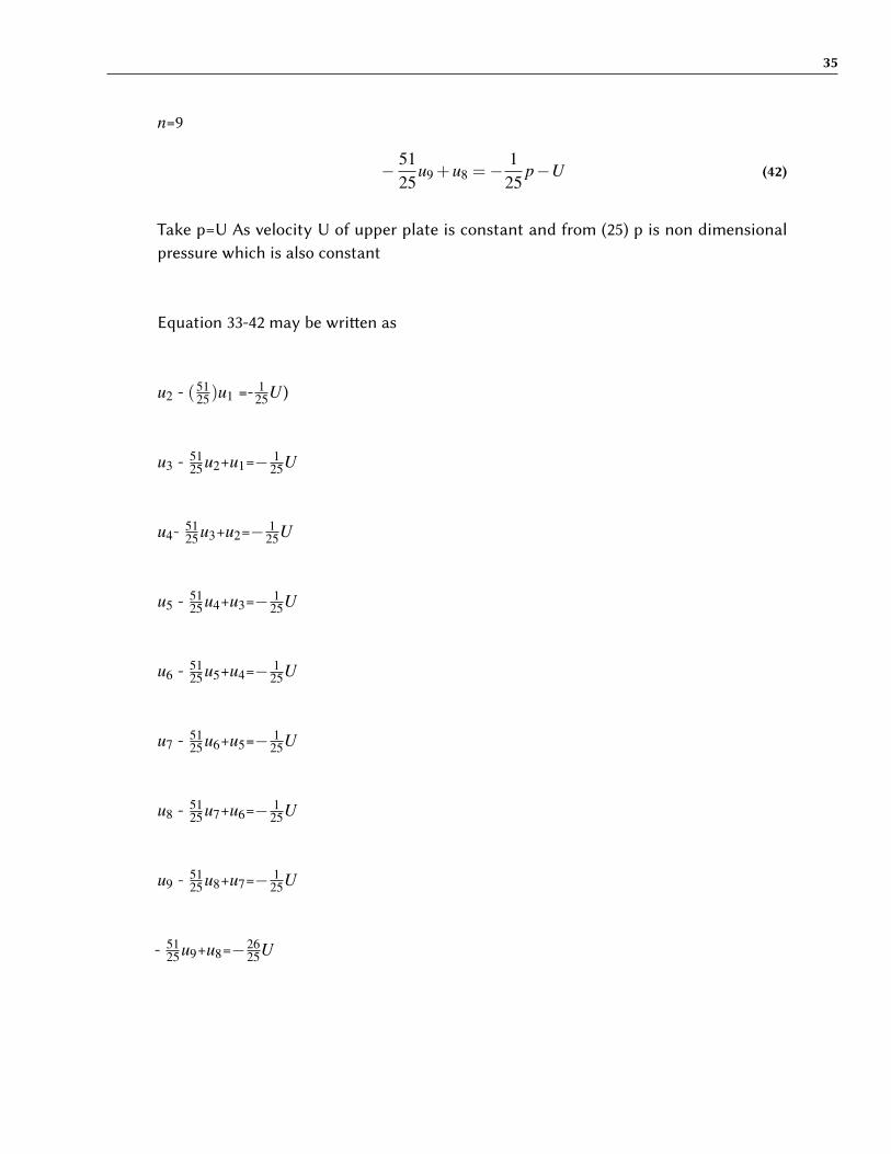
n=9

− 5125

u9 +u8 =−1

25p−U (42)

Take p=U As velocity U of upper plate is constant and from (25) p is non dimensionalpressure which is also constant

Equation 33-42 may be wri�en as

u2 - (5125)u1 =- 1

25U )

u3 - 5125u2+u1=− 1

25U

u4- 5125u3+u2=− 1

25U

u5 - 5125u4+u3=− 1

25U

u6 - 5125u5+u4=− 1

25U

u7 - 5125u6+u5=− 1

25U

u8 - 5125u7+u6=− 1

25U

u9 - 5125u8+u7=− 1

25U

- 5125u9+u8=−26

25U

36

Which can be wri�en in matrix form as

−5125 1 0 0 0 0 0 0 0

1 −5125 1 0 0 0 0 0 0

0 1 −5125 1 0 0 0 0 0

0 0 1 −5125 1 0 0 0 0

0 0 0 1 −5125 1 0 0 0

0 0 0 0 1 −5125 1 0 0

0 0 0 0 0 1 −5125 1 0

0 0 0 0 0 0 1 −5125 1

0 0 0 0 0 0 0 1 −5125

u1

u2

u3

u4

u5

u6

u7

u8

u9

=

− 125U

− 125U

− 125U

− 125U

− 125U

− 125U

− 125U

− 125U

−2625U

Using row reduction formula the above matrix can be reduced to

1 0 0 0 0 0 0 0 0

0 1 0 0 0 0 0 0 0

0 0 1 0 0 0 0 0 0

0 0 0 1 0 0 0 0 0

0 0 0 0 1 0 0 0 0

0 0 0 0 0 1 0 0 0

0 0 0 0 0 0 1 0 0

0 0 0 0 0 0 0 1 0

0 0 0 0 0 0 0 0 1

u1

u2

u3

u4

u5

u6

u7

u8

u9

=

0.1886U

0.3446U

0.4745U

0.5834U

0.6756U

0.7548U

0.8242U

0.8866U

0.9444U

u1U = 0.1886 ; u2

U = 0.3446 ; u3U = 0.4745

u4U = 0.5834 ; u5

U = 0.6756 ; u6U = 0.7548

u7U = 0.8242 ; u8

U = 0.8866 ; u9U = 0.9444

37

CASE 2 M=1;Taking α=60sin2(60)=3

4

un+1−2un +un−1 - h2M2sin2αun=-ph2

un+1−2un +un−1 - 3100un=-p 1

25

un+1-203100un+un−1 =- 1

25 p

P=U

n=1 : u2 - (203100)u1 =- 1

25U )

n=2 : u1 - 203100u2+u3=− 1

25U

n=3 : u2- 203100u3+u4=− 1

25U

n=4 : u3 - 203100u4+u5=− 1

25U

n=5 : u4 - 203100u5+u6=− 1

25U

n=6 : u5 - 203100u6+u7=− 1

25U

n=7 :u6 - 203100u7+u8=− 1

25U

n=8 : u7 - 203100u8+u9=− 1

25U

n=9 : u8- 203100u9=−26

25U

Which can be wri�en as

38

−203100 1 0 0 0 0 0 0 0

1 −203100 1 0 0 0 0 0 0

0 1 −203100 1 0 0 0 0 0

0 0 1 −203100 1 0 0 0 0

0 0 0 1 −203100 1 0 0 0

0 0 0 0 1 −203100 1 0 0

0 0 0 0 0 1 −203100 1 0

0 0 0 0 0 0 1 −203100 1

0 0 0 0 0 0 0 1 −203100

u1

u2

u3

u4

u5

u6

u7

u8

u9

=

− 125U

− 125U

− 125U

− 125U

− 125U

− 125U

− 125U

− 125U

−2625U

Using row reduction formula the above matrix can be reduced to

1 0 0 0 0 0 0 0 0

0 1 0 0 0 0 0 0 0

0 0 1 0 0 0 0 0 0

0 0 0 1 0 0 0 0 0

0 0 0 0 1 0 0 0 0

0 0 0 0 0 1 0 0 0

0 0 0 0 0 0 1 0 0

0 0 0 0 0 0 0 1 0

0 0 0 0 0 0 0 0 1

u1

u2

u3

u4

u5

u6

u7

u8

u9

=

0.2056U

0.3774U

0.5206U

0.6393U

0.7372U

0.8173U

0.8818U

0.9328U

0.9718U

U just a constant

u1U =0.2056 ;; u2

U =0.3774 ; u3U =0.5206

u4U =0.6393 ; u5

U =0.7372 ; u6U =0.8173

39

u7U =0.8818; u8

U =0.9328; u9U =0.9718

CASE 3 Taking α=45sin2(45)=1

2

un+1−2un +un−1 - h2M2sin2αun=-ph2

un+1−2un +un−1 - 150un=-p 1

25

un+1-10150 un+un−1 =- 1

25 p

P=U

n=1 : u2 - (10150 )u1 =- 1

25U )

n=2 : u1 - 10150 u2+u3=− 1

25U

n=3 :u2 - 10150 u3+u4=− 1

25U

n=4 : u3 - 10150 u4+u5=− 1

25U

n=5 : u4 - 10150 u5+u6=− 1

25U

n=6 :u5 - 10150 u6+u7=− 1

25U

n=7 : u6 - 10150 u7+u8=− 1

25U

n=8 : u7 - 10150 u8+u9=− 1

25U

n=9 : u8- 10150 u9=−26

25U

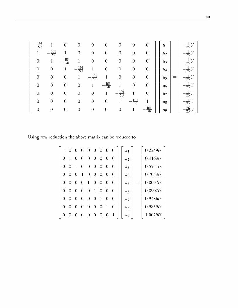
which can be writen as

40

−10150 1 0 0 0 0 0 0 0

1 −10150 1 0 0 0 0 0 0

0 1 −10150 1 0 0 0 0 0

0 0 1 −10150 1 0 0 0 0

0 0 0 1 −10150 1 0 0 0

0 0 0 0 1 −10150 1 0 0

0 0 0 0 0 1 −10150 1 0

0 0 0 0 0 0 1 −10150 1

0 0 0 0 0 0 0 1 −10150

u1

u2

u3

u4

u5

u6

u7

u8

u9

=

− 125U

− 125U

− 125U

− 125U

− 125U

− 125U

− 125U

− 125U

−2625U

Using row reduction the above matrix can be reduced to

1 0 0 0 0 0 0 0 0

0 1 0 0 0 0 0 0 0

0 0 1 0 0 0 0 0 0

0 0 0 1 0 0 0 0 0

0 0 0 0 1 0 0 0 0

0 0 0 0 0 1 0 0 0

0 0 0 0 0 0 1 0 0

0 0 0 0 0 0 0 1 0

0 0 0 0 0 0 0 0 1

u1

u2

u3

u4

u5

u6

u7

u8

u9

=

0.2259U

0.4163U

0.5751U

0.7053U

0.8097U

0.8902U

0.9486U

0.9859U

1.0029U

41

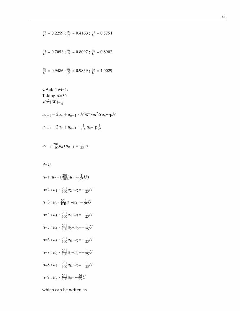
u1U = 0.2259 ; u2

U = 0.4163 ; u3U = 0.5751

u4U = 0.7053 ; u5

U = 0.8097 ; u6U = 0.8902

u7U = 0.9486 ; u8

U = 0.9859 ; u9U = 1.0029

CASE 4 M=1;Taking α=30sin2(30)=1

4

un+1−2un +un−1 - h2M2sin2αun=-ph2

un+1−2un +un−1 - 1100un=-p 1

25

un+1-201100un+un−1 =- 1

25 p

P=U

n=1 :u2 - (201100)u1 =- 1

25U )

n=2 : u1 - 201100u2+u2=− 1

25U

n=3 : u2- 201100u3+u4=− 1

25U

n=4 : u3 - 201100u4+u5=− 1

25U

n=5 : u4 - 201100u5+u6=− 1

25U

n=6 : u5 - 201100u6+u7=− 1

25U

n=7 : u6 - 201100u7+u8=− 1

25U

n=8 : u7 - 201100u8+u9=− 1

25U

n=9 : u8 - 201100u9=−26

25U

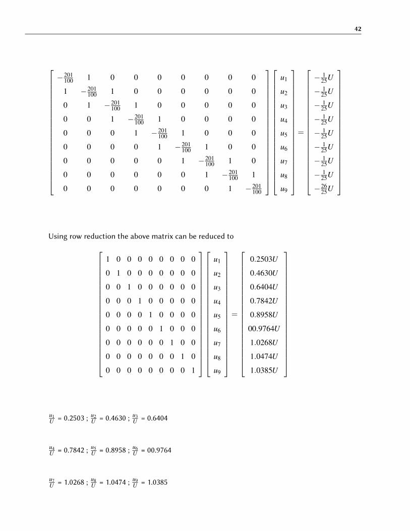
which can be writen as

42

−201100 1 0 0 0 0 0 0 0

1 −201100 1 0 0 0 0 0 0

0 1 −201100 1 0 0 0 0 0

0 0 1 −201100 1 0 0 0 0

0 0 0 1 −201100 1 0 0 0

0 0 0 0 1 −201100 1 0 0

0 0 0 0 0 1 −201100 1 0

0 0 0 0 0 0 1 −201100 1

0 0 0 0 0 0 0 1 −201100

u1

u2

u3

u4

u5

u6

u7

u8

u9

=

− 125U

− 125U

− 125U

− 125U

− 125U

− 125U

− 125U

− 125U

−2625U

Using row reduction the above matrix can be reduced to

1 0 0 0 0 0 0 0 0

0 1 0 0 0 0 0 0 0

0 0 1 0 0 0 0 0 0

0 0 0 1 0 0 0 0 0

0 0 0 0 1 0 0 0 0

0 0 0 0 0 1 0 0 0

0 0 0 0 0 0 1 0 0

0 0 0 0 0 0 0 1 0

0 0 0 0 0 0 0 0 1

u1

u2

u3

u4

u5

u6

u7

u8

u9

=

0.2503U

0.4630U

0.6404U

0.7842U

0.8958U

00.9764U

1.0268U

1.0474U

1.0385U

u1U = 0.2503 ; u2

U = 0.4630 ; u3U = 0.6404

u4U = 0.7842 ; u5

U = 0.8958 ; u6U = 00.9764

u7U = 1.0268 ; u8

U = 1.0474 ; u9U = 1.0385

43

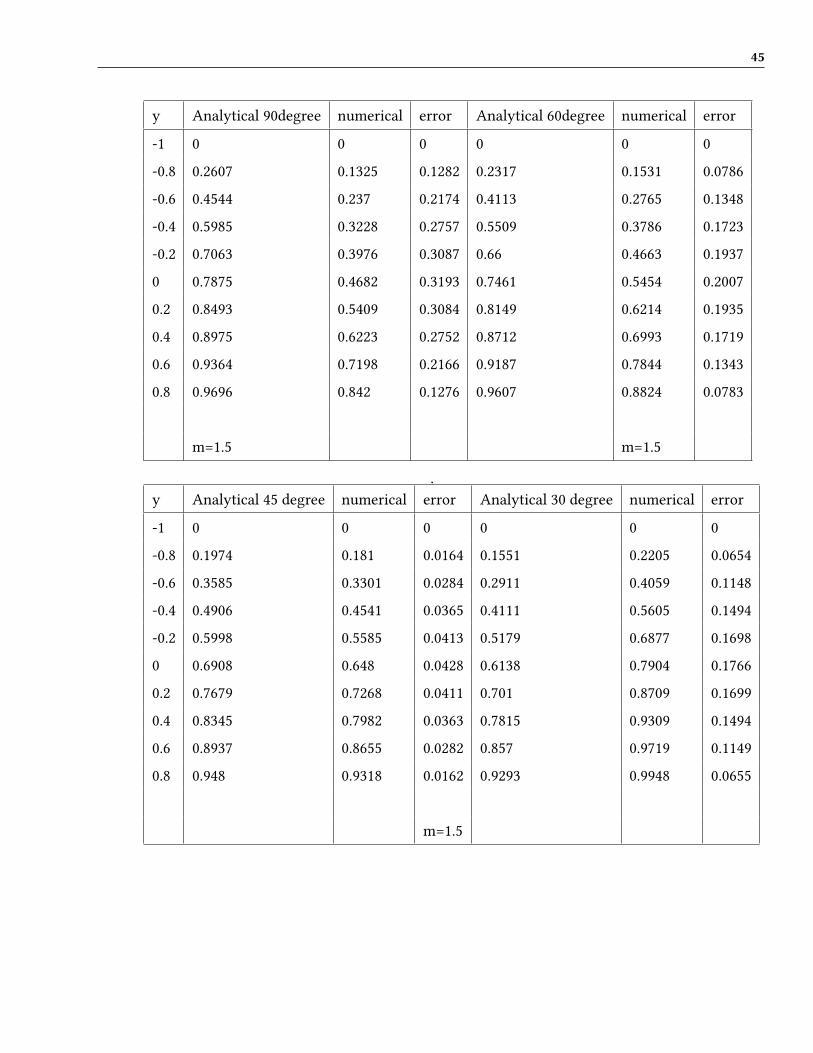
Using the above formula to calculate m=1.5 m= 2 ,the following tables will be obtained

m=1.5

44

Y excact numerical error analytical numerical error

-1 0 0 0 0 0 0

-0.8 0.1888 0.1886 0.001059322 0.1703 0.2056 0.0353

-0.6 0.345 0.3446 0.00115942 0.3156 0.3774 0.0618

-0.4 0.4749 0.4745 0.000842283 0.4404 0.5206 0.0802

-0.2 0.5838 0.5834 0.000685166 0.5483 0.6393 0.091

0 0.676 0.6756 0.000591716 0.6426 0.7372 0.0946

0.2 0.7551 0.7548 0.000397298 0.7262 0.8173 0.0911

0.4 0.8245 0.8242 0.000363857 0.8015 0.8818 0.0803

0.6 0.8867 0.8866 0.000112778 0.8709 0.9328 0.0619

0.8 0.9445 0.9444 0.000105876 0.9364 0.9718 0.0354

1 1 1 0 1 1 0

α=90 α=60

.

Y analyrical numerical error analytical numerical error

-1 0 0 0 0 0 0

-0.8 0.1497 0.2259 0.0762 0.1265 0.2503 0.1238

-0.6 0.2824 0.4163 0.1339 0.2443 0.463 0.2187

-0.4 0.4007 0.5751 0.1744 0.3545 0.6404 0.2859

-0.2 0.507 0.7053 0.1983 0.4583 0.7842 0.3259

0 0.6034 0.8097 0.2063 0.5566 0.8958 0.3392

0.2 0.6918 0.8902 0.1984 0.6505 0.9764 0.3259

0.4 0.7741 0.9486 0.1745 0.7409 1.0268 0.2859

0.6 0.8519 0.9859 0.134 0.8287 1.0474 0.2187

0.8 0.9267 1.0029 0.0762 0.9148 1.0385 0.1237

1 1 1 0 1 1 0

α=45 α=30

45

y Analytical 90degree numerical error Analytical 60degree numerical error

-1 0 0 0 0 0 0

-0.8 0.2607 0.1325 0.1282 0.2317 0.1531 0.0786

-0.6 0.4544 0.237 0.2174 0.4113 0.2765 0.1348

-0.4 0.5985 0.3228 0.2757 0.5509 0.3786 0.1723

-0.2 0.7063 0.3976 0.3087 0.66 0.4663 0.1937

0 0.7875 0.4682 0.3193 0.7461 0.5454 0.2007

0.2 0.8493 0.5409 0.3084 0.8149 0.6214 0.1935

0.4 0.8975 0.6223 0.2752 0.8712 0.6993 0.1719

0.6 0.9364 0.7198 0.2166 0.9187 0.7844 0.1343

0.8 0.9696 0.842 0.1276 0.9607 0.8824 0.0783

m=1.5 m=1.5

.

y Analytical 45 degree numerical error Analytical 30 degree numerical error

-1 0 0 0 0 0 0

-0.8 0.1974 0.181 0.0164 0.1551 0.2205 0.0654

-0.6 0.3585 0.3301 0.0284 0.2911 0.4059 0.1148

-0.4 0.4906 0.4541 0.0365 0.4111 0.5605 0.1494

-0.2 0.5998 0.5585 0.0413 0.5179 0.6877 0.1698

0 0.6908 0.648 0.0428 0.6138 0.7904 0.1766

0.2 0.7679 0.7268 0.0411 0.701 0.8709 0.1699

0.4 0.8345 0.7982 0.0363 0.7815 0.9309 0.1494

0.6 0.8937 0.8655 0.0282 0.857 0.9719 0.1149

0.8 0.948 0.9318 0.0162 0.9293 0.9948 0.0655

m=1.5

46

y ANALYTIC 90DEGREE Numerical error ANALYTIC 60DEGREE Numerical error

-1 0 0 0 0 0 0

-0.8 0.33 0.0936 0.2364 0.2935 0.1124 0.1999

-0.6 0.5513 0.1621 0.3892 0.5013 0.1982 0.3392

-0.4 0.6998 0.2166 0.4832 0.6487 0.2679 0.4321

-0.2 0.7997 0.2657 0.534 0.7535 0.3296 0.4878

0 0.8671 0.3173 0.5498 0.8284 0.391 0.5111

0.2 0.913 0.3797 0.5333 0.8826 0.4592 0.5029

0.4 0.9447 0.4628 0.4819 0.9225 0.5426 0.4597

0.6 0.9675 0.58 0.3875 0.953 0.6511 0.373

0.8 0.9849 0.75 0.2349 0.9779 0.7977 0.2279

1 1 1 0 1 1 0

.

y ANALYTIC 45DEGREE Numerical error ANALYTIC 30DEGREE Numerical error

-1 0 0 0 0 0 0

-0.8 0.2484 0.1409 0.1075 0.1888 0.1886 0.0002

-0.6 0.4362 0.2532 0.183 0.345 0.3446 0.0004

-0.4 0.5786 0.3457 0.2329 0.4749 0.4745 0.0004

-0.2 0.6871 0.4258 0.2613 0.5838 0.5834 0.0004

0 0.7705 0.5 0.2705 0.676 0.6756 0.0004

0.2 0.8353 0.5742 0.2611 0.7551 0.7548 0.0003

0.4 0.8868 0.6543 0.2325 0.8245 0.8242 0.0003

0.6 0.9293 0.7468 0.1825 0.8867 0.8866 1E-04

0.8 0.966 0.8591 0.1069 0.9445 0.9444 1E-04

1 1 1 1 1 0

m=2

47

48

49

50

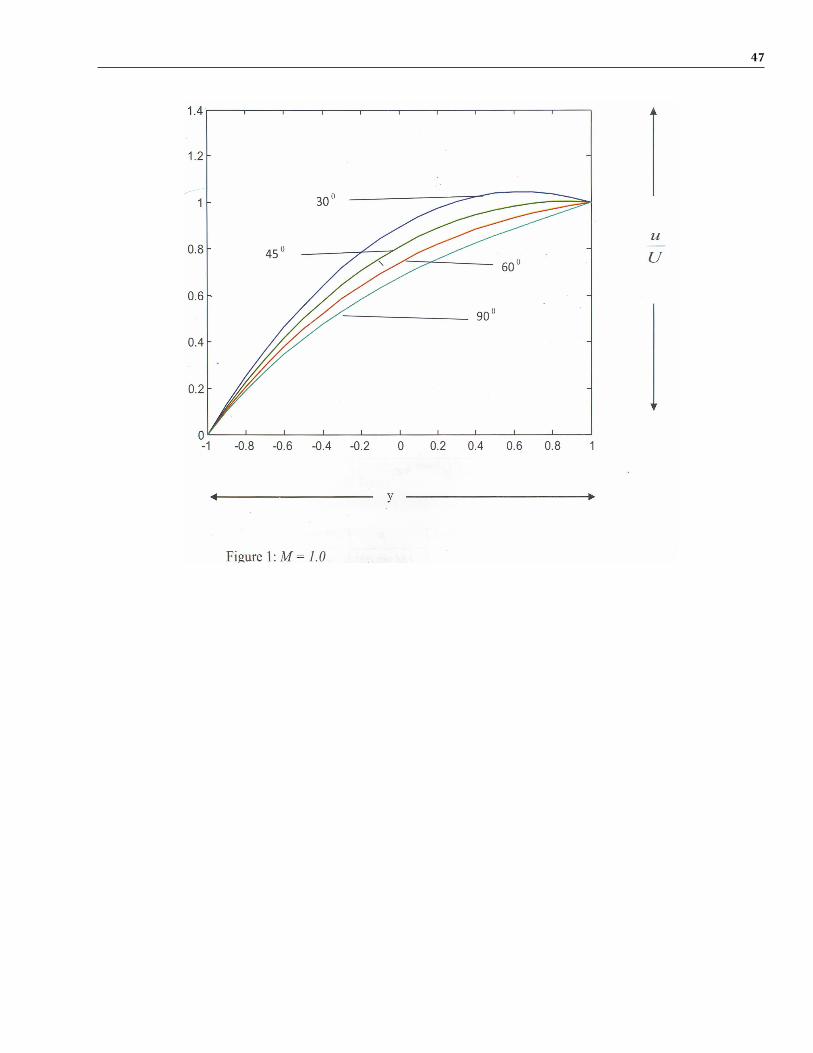
4 DISCUSSION OF RESULTS ANDAPPLICATIONS

The problem has been solved by the central di�erence method with 10 equal mesh pointand step size of 0.2 An analytic expression for the velocity of fluid particle has beenobtained. It is clear from equation (34) that if we take applied pressure gradient P =0 then we get problem of Singh (2007) as a particular case of present problem. table 1to 6 are calculated at the inclinations of 30 degree,45 degree,60 degree and 90 degree. It is clear from the tables that velocity decreases as the strength of magnetic field isincreased. Also evident is the fact that with the increase of inclination of magnetic field,there is a decrease in the velocity profile. Again velocity profiles at 90 degree gives usthe steady hydro magnetic flow of viscous in compressible fluid under applied pressuregradient and when upper plate is also moving with constant velocity under the influenceof transverse magnetic field as a particular case of present problem. It is evident from(34) that when U = 0 then the problem of magneto hydrodynamic steady flow of liquidbetween parallel plates Singh (1993) can be obtained as a particular case of this problem.The results obtained here can be applied to the designs and operations of MHD generator,MHD pump, electromagnetic flow meter, and to crude oil

51

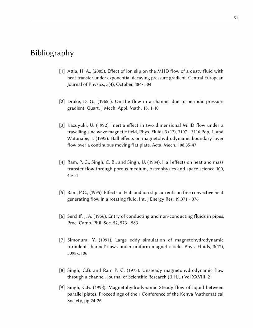
Bibliography

[1] A�ia, H. A., (2005). E�ect of ion slip on the MHD flow of a dusty fluid withheat transfer under exponential decaying pressure gradient. Central EuropeanJournal of Physics, 3(4), October, 484- 504

[2] Drake, D. G., (1965 ). On the flow in a channel due to periodic pressuregradient. �art. J Mech. Appl. Math. 18, 1-10

[3] Kazuyuki, U. (1992). Inertia e�ect in two dimensional MHD flow under atravelling sine wave magnetic field, Phys. Fluids 3 (12), 3107 - 3116 Pop, 1. andWatanabe, T. (1995). Hall e�ects on magnetohydrodynamic boundary layerflow over a continuous moving flat plate. Acta. Mech. 108,35-47

[4] Ram, P. C., Singh, C. B., and Singh, U. (1984). Hall e�ects on heat and masstransfer flow through porous medium, Astrophysics and space science 100,45-51

[5] Ram, P.C., (1995). E�ects of Hall and ion slip currents on free convective heatgenerating flow in a rotating fluid. Int. J Energy Res. 19,371 - 376

[6] Sercli�, J. A. (1956). Entry of conducting and non-conducting fluids in pipes.Proc. Camb. Phil. Soc. 52, 573 - 583

[7] Simonura, Y. (1991). Large eddy simulation of magnetohydrodynamicturbulent channel"flows under uniform magnetic field. Phys. Fluids, 3(12),3098-3106

[8] Singh, C.B. and Ram P. C. (1978). Unsteady magnetohydrodynamic flowthrough a channel. Journal of Scientific Research (B.H.U) Vol XXVIII, 2

[9] Singh, C.B. (1993). Magnetohydrodynamic Steady flow of liquid betweenparallel plates. Proceedings of the r Conference of the Kenya MathematicalSociety, pp 24-26

52

[10] Singh, CB. (1998). Unsteady magneto hydrodynamic flow of liquid through achannel under variable pressure gradient. K.JS Series A, 11(1), 69 - 78

[11] Singh, CB. (2000). Unsteady flow of liquid through a channel with pressuregradient changing exponentially under the influence of inclined magneticfield, International Journal of BioChemiPhysic, 1037 - 40

[12] Singh, C. B. (2007). Hydromagnetic steady flow of viscous incompressible fluidbetween two parallel infinite plates under the influence of inclined magneticfield, KJ.S. Series A, 12(1)