numerical solution of non–linear conservation laws · 2.2. scalar conservation laws 5 (2.5) as...

EÖTVÖS LORÁND UNIVERSITY

MASTER’S THESIS

Numerical Solution of Non–LinearConservation Laws

Author:Nor El Houda SERIDI

Supervisor:Dr. Ferenc IZSÁK

Applied mathematics (MSc)

Department of Applied Analysis and Computational Mathematics

Institute of MathematicsFaculty of Science

June, 2017

http://www.elte.hu/en

http://www.cs.elte.hu/~izsakf

http://www.cs.elte.hu/?lang=en

http://science.elte.hu/

iii

Eötvös Loránd University

AbstractFaculty of Science

Institute of Mathematics

Applied mathematics (MSc)

Numerical Solution of Non–Linear Conservation Laws

by Nor El Houda SERIDI

Conservation laws, which are conservative systems of hyperbolic differentialequations result from continuum mechanics (e.g. the equations of shallowwater waves, fluid dynamics, magneto-fluid dynamics and certain elasticityproblems).In this work, we will start with a general introduction and show how theyarise from the basic principles of physics. We will discuss the non-uniquenessof the solution in general, and later we will show how the entropy conditioncan deal with this problem. We will study an other interesting fact, whichis the non-smoothness of the solution, that makes the numerical treatmenthard.Besides these two difficulties, we will find a special difficulty when we willconstruct the numerical schemes, which is the physical structure of the origi-nal problem namely the conservation, that leads us to define the conservativeschemes in order to preserve this property.We will discuss the Lax–Wendroof and Godunov schemes and their prop-erties, turning to the high order nonlinear schemes MUSCL, which will beobtained by applying a non-oscillatory first order accurate scheme to an ap-propriately modified flux function. We will study van Leer’s scheme andwe want to make it more accurate by avoiding oscillations. For this we willuse TVD schemes, which are free of oscillation and define the slope limiters.We will state most popular second order limiters: van Leer, minmod and su-perbee limiters. We end this work with some numerical experiments whichdemonstrate the performance of these schemes.

http://www.elte.hu/en

http://science.elte.hu/

http://www.cs.elte.hu/?lang=en

v

AcknowledgementsI would like to thank all people helped in this work directly or indirectly.

One of these people is my advisor Mr. Ferenc Iszak who directly con-tributed in this work by his wise advices, remarks and feedback. He alwayscares about this work and gives it from his time. He was kind and helpful.I thank him not as a tradition I thank him because really he merits it.

I acknowledge my parents who provide me with love, care and the infi-nite support.

vii

Contents

Abstract iii

Acknowledgements v

1 Introduction 1

2 Preliminaries to Conservation Laws 32.1 Conservation laws . . . . . . . . . . . . . . . . . . . . . . . . . 3

2.1.1 Integral and differential form . . . . . . . . . . . . . . . 42.2 Scalar conservation laws . . . . . . . . . . . . . . . . . . . . . . 5

2.2.1 The linear advection equation . . . . . . . . . . . . . . . 52.2.2 Burgers’s equation . . . . . . . . . . . . . . . . . . . . . 6

2.3 Classical solution of conservation laws . . . . . . . . . . . . . 62.3.1 Classical solution . . . . . . . . . . . . . . . . . . . . . . 62.3.2 Weak solution . . . . . . . . . . . . . . . . . . . . . . . . 72.3.3 Riemann problem and Rankine–Hugoniot jump condi-

tion . . . . . . . . . . . . . . . . . . . . . . . . . . . . . . 82.4 Manipulating conservation laws . . . . . . . . . . . . . . . . . 10

3 Numerical Methods for Conservation Laws 113.1 Finite difference method . . . . . . . . . . . . . . . . . . . . . . 123.2 Conservative schemes . . . . . . . . . . . . . . . . . . . . . . . 13

3.2.1 Lax–Wendroff’s method . . . . . . . . . . . . . . . . . . 153.2.2 Godunov’s method . . . . . . . . . . . . . . . . . . . . . 16

4 Higher order and TVD methods 194.1 MUSCL- higher order methods . . . . . . . . . . . . . . . . . . 19

4.1.1 Van Leer’s method for advection and Burger’s equa-tions . . . . . . . . . . . . . . . . . . . . . . . . . . . . . 22Van Leer’s method for advection equation . . . . . . . 22

Van Leer method for Burgers’s equation . . . . . . . . . 234.1.2 Slope Limiter . . . . . . . . . . . . . . . . . . . . . . . . 24

Van Leer’s limiter . . . . . . . . . . . . . . . . . . . . . . 25Minmod limiter . . . . . . . . . . . . . . . . . . . . . . . 25Superbee limiter . . . . . . . . . . . . . . . . . . . . . . 25

5 Numerical Result 27

General Conclusion 33

1

Chapter 1

Introduction

Flow is a phenomena that occurs in many natural and technical environ-ment, in physics, fluid dynamics is a sub-discipline of fluid mechanics thatdescribes the flow of fluids (liquids and gases). Flows are everywhere evenin the our body where flow-dependent transport processes that supply ourbody with the oxygen.Fluid flows in the atmosphere are used to determine whether certain regionscan be used for agriculture, if they are sufficiently supplied with rain. Othernegative effects on our natural environment are the devastations that hur-ricanes and cyclones can cause. This makes it clear that humans not onlydepend on fluid flows in the positive sense, but also have to learn to livewith the effects of such fluid flows that can destroy the entire environment.The above paragraph clearly shows that without fluid flows, life as we knowit will not be possible on earth, our natural and technical world would bedifferent and might not even exist at all.

In physics, several principles state that certain physical properties (mea-surable quantities) do not change in the course of time within an isolatedphysical system.In classical physics, laws of this type govern energy, momentum, angularmomentum, mass and electric charge.In particle physics, other conservation laws are applied to properties of sub-atomic particles that are invariant during interactions.An important function of conservation laws is that they make possible topredict the macroscopic behavior of a system without having to consider themicroscopic details of the course of physical processes or chemical reactions.To analyze and solve problems that involve fluid flows, we need to use andstudy the conservation laws which can be formulated mathematically byintegral or differential equations. The main difficulties faced when solv-ing these problems are the non-uniqueness of the solution which makes ithard to distinguish the physical solution from non-physical onces, the lakeof smoothness of solution which is not required physically and the type ofdomain ( convex or concave).

3

Chapter 2

Preliminaries to Conservation Laws

2.1 Conservation laws

In mathematics, conservation laws are written as a time-dependent hyper-bolic system of partial differential equations, which is usually non-linear in-sert this in one space dimension the equations take the form

∂

∂tu(t, x) +

∂

∂xf(u(t, x)) = 0. (2.1)

Here u : R×R→ Rm is anm-dimensional vector function of conserved quan-tities and f : Rm → Rm is called the flux function.The main assumption underlying the equation (2.1) is that knowing the valueof u(t, x) at a given point and time allows us to determine the rate of flow orflux of each state variable j.The equation (2.1) must be augmented by some initial conditions and alsopossibly boundary conditions on a bounded spatial domain.In two space dimensions a system of conservation laws takes the form

∂

∂tu(t, x, y) +

∂

∂xf(u(t, x, y)) +

∂

∂yg(u(t, x, y)) = 0. (2.2)

Here the flux function is given with the pair (f, g), where f, g : Rm → Rm.There are several reasons for studying this particular class of equations ontheir own in some depth:

• Many practical problems in science and engineering involve conservedquantities and lead to PDEs of this class.

• There are special difficulties associated with solving these systems (e.g.shock formation) that are not seen elsewhere and must be dealt withcarefully in developing numerical methods.

• Although few exact solutions are known, a great deal is known aboutthe mathematical structure of these equations and their solution.

We want to exploit this theory to develop special methods that overcomesome of the above and the numerical difficulties encountered with a morenaive approach.

4 Chapter 2. Preliminaries to Conservation Laws

2.1.1 Integral and differential form

Conservation laws are formulated originally in an integral form. After somedifferential operations, we can arrive to the differential form.

To see how the conservation laws arise from physical principles let usstate the following physical example of conservation mass in a one-dimensionalgas dynamics problem [2].We assume that we have tube where its walls are impermeable and the den-sity ρ and velocity v of the gas are constants across each cross section of thetube.Let x represent the distance along the tube, we can define the mass of gas inthe section [x1, x2] by the following equation:

mass in [x1, x2]at time t =

∫ x2

x1

ρ(t, x) dx. (2.3)

Then the rate of flux of gas past the point x at time t is given by:

mass flux at (t, x) = ρ(t, x)v(t, x).

The rate of change of mass in [x1, x2] is given by the difference in fluxes at x1

and x2d

dt

∫ x2

x1

ρ(t, x) dx = ρ(t, x1)v(t, x1)− ρ(t, x2)v(t, x2), (2.4)

which gives the integral form of conservation laws.In order to derive the differential form of the conservation laws, we assumethat ρ(t, x) and v(t, x) are differentiable functions and integrate the equation(2.4) with respect to time between t1 and t2∫ x2

x1

ρ(t2, x) dx =

∫ x2

x1

ρ(t1, x) dx+

∫ t2

t1

ρ(t, x1)v(t, x1) dt−∫ t2

t1

ρ(t, x2)v(t, x2) dt.

Using the following equations

ρ(t2, x)− ρ(t1, x) =

∫ t2

t1

d

dtρ(t, x) dt,

ρ(t, x2)v(t, x2)− ρ(t, x1)v(t, x1) =

∫ x2

x1

d

dxρ(t, x)v(t, x) dx,

we find ∫ t2

t1

∫ x2

x1

d

dtρ(t, x) +

d

dxρ(t, x)v(t, x) dx dt = 0.

Since this must hold for any section [x1, x2] and any time interval [t1, t2], weobtain

ρt + (ρv)x = 0. (2.5)

In order to solve this equation the velocity, v(t, x) is assumed to be given orknown as a function of the density ρ(t, x), then we can write the equation

2.2. Scalar conservation laws 5

(2.5) as followsρt + f(ρ)x = 0, (2.6)

which gives the differential form of conservation laws.

2.2 Scalar conservation laws

The study of linear conservation laws is important for understanding thebehavior of a numerical scheme, but it is also very important to consider thatthe introduction of the nonlinearity changes dramatically the nature of theproblem because it induces a loss of the uniqueness of the weak solution.

2.2.1 The linear advection equation

In this subsection, we mainly follow the exposition in [2].Let us consider the following Cauchy problem for the linear advection equa-tion on the domain x ∈ (−∞,∞), t ∈ R+

ut + (a(x)u)x = 0.

u(t, x) = u0(x).(2.7)

Here a(x) is a smooth function representing the velocity.Let us assume that a is a constant and u0 is a given function.The exact solution for this problem is:

u(t, x) = u0(x− at).

As time evolves, the initial data simply propagates unchanged to the right ifthe velocity a > 0 or to the left if a < 0 .The solution u(t, x) is constant along each ray x− at = x0, which are knownas the characteristics of the equation.The characteristics are curves t → (t, x(t)) which satisfy the ordinary differ-ential equation {

x′(t) = a,

x(0) = x0.

If we differentiate u(t, x) along one of these curves to find the rate of changeof u along the characteristics, we find that

d

dtu(t, x(t)) =

∂

∂xu(t, x(t)) +

∂

∂tu(t, x(t))x′(t)

= ut + aux

= 0,

confirming that u is constant along these characteristics.If the initial data u0 is non differentiable then u is not a classical solution forthe PDE any more, however this function u does satisfy the integral form.One can suggest to approximate the non smooth initial data u0 to a sequence


of smooth functions, but unfortunately this does not work for nonlinear prob-lems.

2.2.2 Burgers’s equation

The most famous case is Burgers’s equation, in which the flux f(u) = 12u2,

then the problem can be written as

ut + uux = 0. (2.8)

We can construct the solution of this problem with a smooth initial conditionby the following characteristics

x′(t) = u(t, x(t)),

where u is constant along each characteristic, such that the slope x′(t) is con-stant. So the characteristics are straight lines determined by the initial data.If u(t, ·) is smooth then the characteristics do not cross and we can solve theequation x = ξ + u(0, ξ)t for ξ and then u(t, x) = (ξ, 0).This is true for small t but for large t the equation x = ξ + u(0, ξ)t may havemore solutions. This happens when the characteristics cross each other andthe PDE does not have any more classical solution and the weak solution (wehope to determined) becomes discontinuous, (for more details, see [1], and[2]).For some initial condition the function can become multivalued in one point,which is impossible to happen in the physics.

2.3 Classical solution of conservation laws

Before turning to the numerical approximation of the solution, we have tosee whether the problem is well posed or not (existence and uniqueness).We start with the classical solution.

2.3.1 Classical solution

Consider the following Cauchy problem of conservation laws{ut + f(u, t)x = 0 x ∈ R, t > 0,

u(0, x) = u0 x ∈ R, t = 0.(2.9)

If u0(x) is increasing, (decreasing) and f(u) is convex, ( concave), the classicalsolution of this problem (2.9) well defined for all t > 0.However, in the general case, classical solutions fail to exist for all t > 0even if u0 is very smooth. This happens when infx u

′0(x) f ′′(u0(x)) < 0, then

2.3. Classical solution of conservation laws 7

classical solutions exist only for t in [0, T ∗] where

T ∗ =1

infx u′0(x)f ′′(u0(x)).

At the time t = T ∗ the characteristics first cross which lead the function u(x, t)to have an infinite slope and forms a shock [2].

Proof. Since along characteristics u(x(t), t) is equal to u0(x0), we can writex(t) = x0 + tf ′(u0(x0)). We can calculate the first time when two differentcharacteristics arrive at same point (x, t).In this case there are two points x0 and x0 such that

x = x0 + tf ′(u0(x0)) = x0 + tf ′(u0(x0)),

which implies that

t =x0 − x0

f ′(u0(x0))− f ′(u0(x0))

=1

f ′(u0(x0))−f ′(u0(x0))x0−x0

=1

u′0(ξ)f ′′(u0(ξ)),

where ξ lies between x0 and x0. Obviously, this expression for t makes sensewhen 1

u′0(ξ)f ′′(u0(ξ))is negative. Thus, the blow up occurs if u′0(ξ)f ′′(u0(ξ)) is

somewhere negative at T ∗ and the solution forms a shock wave.

Since the classical solution may not exist for large t, let us consider theweak solution.

2.3.2 Weak solution

To define a generalized solution which does not require differentiability is togo back to the integral form, and assume that u(t, x) is a generalized solutionif it satisfies the following equation for all x1, x2, t1, t2∫ t2

t1

∫ x2

x1

d

dtu(t, x) +

d

dxf(u(t, x)) dx dt = 0.

In our case we will use a continuously differentiable test function with com-pacted support φ ∈ C1

0(R×R), we multiply our PDE by this test function andintegrate once with respect to the space and once with respect to the time∫ +∞

0

∫ +∞

−∞φut + φfx(u) = 0.

Using integration by part,∫ +∞

0

∫ +∞

−∞φtu+ φxf(u) =

∫ +∞

−∞φ(0, x)u(0, x). (2.10)


Definition 1. The measurable and bounded function u(t, x) called a weaksolution of the conservation laws if it satisfies the equation (2.10) for all func-tions φ ∈ C1

0(R× R+).

Rewrite the integral form of conservation laws which is the original equa-tion we want to solve,∫ x2

x1

u(t2, x) dx =

∫ x2

x1

u(t1, x) dx+

∫ t2

t1

f(t, x1) dt−∫ t2

t1

f(t, x2) dt. (2.11)

We give the difference between the original integral and the integral of weaksolution in the following table,

Integral Domain check thatOriginal (2.11) arbitrary rectangle Holds for all x1, x2, t1, t2Weak solution (2.10) fixed domain Holds for all φ ∈ C1

0(R× R+)

Mathematically the two integral forms are equivalent and we should rightlyexpect a more direct connection between the two that does not involve thedifferential equation [2]. This can be achieved by considering special testfunctions φ(x, t) with the property that

φ(t, x) =

{1 for (t, x) ∈ [t1, t2]× [x1, x2]

0 for (t, x) /∈ [t1 − ε, t2 + ε]× [x1 − ε, x2 + ε],(2.12)

with φ smooth in the intermediate strip of width ε. Then φx = φt = 0 exceptin this strip and so the integral (2.10) reduces to an integral over this strip.Unfortunately, it turns out that the weak solutions are often not unique andwe can not distinguish between the physical solution and non-physical solu-tion [2].

2.3.3 Riemann problem and Rankine–Hugoniot jump condi-tion

The conservation law together with piecewise constant data having a singlediscontinuity is known as Riemann problem, (see [1] and [2]).Consider Burgers’s equation with piecewise constant initial data

ut + uux = 0 ; u(0, x) =

{ul x < 0

ur x > 0.(2.13)

We can distinct two cases.

2.3. Classical solution of conservation laws 9

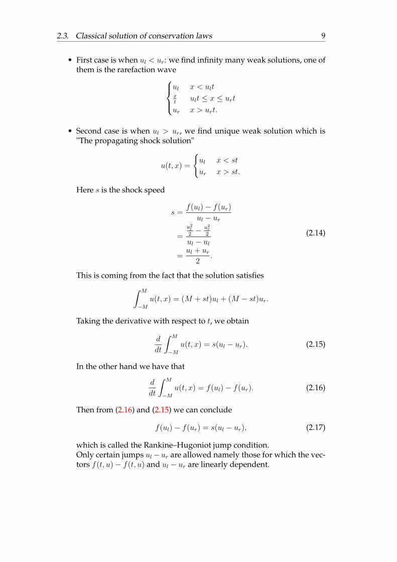
• First case is when ul < ur: we find infinity many weak solutions, one ofthem is the rarefaction wave

ul x < ultxt

ult ≤ x ≤ urt

ur x > urt.

• Second case is when ul > ur, we find unique weak solution which is"The propagating shock solution"

u(t, x) =

{ul x < st

ur x > st.

Here s is the shock speed

s =f(ul)− f(ur)

ul − ur

=

u2l2− u2r

2

ul − ul=ul + ur

2.

(2.14)

This is coming from the fact that the solution satisfies∫ M

−Mu(t, x) = (M + st)ul + (M − st)ur.

Taking the derivative with respect to t, we obtain

d

dt

∫ M

−Mu(t, x) = s(ul − ur). (2.15)

In the other hand we have that

d

dt

∫ M

−Mu(t, x) = f(ul)− f(ur). (2.16)

Then from (2.16) and (2.15) we can conclude

f(ul)− f(ur) = s(ul − ur), (2.17)

which is called the Rankine–Hugoniot jump condition.Only certain jumps ul− ur are allowed namely those for which the vec-tors f(t, u)− f(t, u) and ul − ur are linearly dependent.


2.4 Manipulating conservation laws

One danger to observe in dealing with conservation laws is that transformingthe differential form into what appears to be an equivalent differential equa-tion may not give an equivalent equation in the context of weak solutions[2].

Example 2.4.1. If we multiply Burgers’s equation

ut +

(1

2u2

)x

= 0 (2.18)

by 2u, we obtain an equivalent equation 2uut + 2u2ux = 0 which can be rewrittenas

(u2)t +

(2

3u3

)x

= 0. (2.19)

This is again a conservation law for u2 rather than u itself, with flux functionf(u2) = 2

3(u2)

32 . The differential equations (2.18) and (2.19) have precisely the

same smooth solutions, However, they have different weak solutions, as we can seeby considering the Riemann problem with ul > ur. The unique weak solution ofBurgers’s equation is a shock traveling at speed

s1 =2

3

(u3r − u3

l

u2r + u2

l

)(2.20)

whereas the unique weak solution to manipulated Burgers’s equation is a shock trav-eling at speed

s2 =1

2(ul + ur), (2.21)

and so s1 6= s2 when ul 6= ur, and the two equations have different weak solutions.

This example clearly shows that to manipulate a conservation laws prob-lem the smoothness is required to have equivalent week solution and do notcontradict with the fact that they have same smooth solution but differentweek solution.

11

Chapter 3

Numerical Methods forConservation Laws

The previous chapter gave an overlook about the structure of conservationlaws and its classical solution, and the difficulties which we faced when wewant to solve this kind of problems. This leads us to think on the numericalsolution.Solving such a problem numerically means that, we find approximation toits solution at a finite number of points of the intervals [0, T ] and [xl, xr], sayat the grid points of the following uniform discretization

{0 = t0 < t1 < · · · < tM = T | δ = ∆t = tn+1 − tn}, ∀n = 1, M − 1

{xl = x0 < x1 < · · · < xN = xr | h = ∆x = xj+1 − xj} ∀ j = 1, N − 1.

Denote by unj ≈ u(tn, xj) the approximation of the function u at the point(tn, xj).

The numerical methods have their own difficulties as well, where can giveeither a catastrophic result or work with rate of accuracy at most one.In this chapter we will stat different numerical methods, and explain in de-tails the physical reason of their results, and improve these methods in orderto get more accurate method, which preserve the physical structure of ourproblem.Some features we would like such a method to possess are:

• At least second order accuracy on smooth solutions, and also in smoothregions of a solution even when discontinuities are present elsewhere.

• Sharp resolution of discontinuities without excessive smearing.

• The absence of spurious oscillations in the computed solution.

• An appropriate form of consistency with the weak form of the conser-vation law, required if we hope to converge to weak solutions.

• Nonlinear stability bounds that, together with consistency, allow us toprove convergence as the grid is refined.

12 Chapter 3. Numerical Methods for Conservation Laws

3.1 Finite difference method

The finite difference methods, are a well known methods for solving numer-ically a partial differential equations. In the following, we will discuss anexample to show that the finite difference methods can be useless for conser-vation laws.

Example 3.1.1. Consider Burgers equation with the following initial condition

∂tu(t, x) + u(t, x)∂xu(t, x) = 0

u(0, x) =

{1 if x < 0

0 if x > 0.

(3.1)

We want to approximate this problem using the backward finite difference scheme forthis using the finite differences

∂tu ≈un+1k − unk

δ,

∂xu ≈unk − unk−1

h.

(3.2)

We obtainun+1k − unk

δ+ unk

unk − unk−1

h= 0. (3.3)

Which can be rearranged to get the scheme

un+1k = unk −

δ

hunk(unk − unk−1

).

Compute this scheme with the above initial condition

u1k = u0

k −δ

hu0k

(u0k − u0

k−1

)= 0.

If u0k = 1⇒ u0

k−1 = 1⇒ δhu0k

(u0k − u0

k−1

)= 0.

If u0k = 1⇒ δ

hu0k

(u0k − u0

k−1

)= 0.

So for this initial condition our scheme for the first iteration will be u1k = u0

k whichis not correct.

Remark 1. We can find the exact solution of this problem (3.1) using Riemannproblem.

The above example clearly shows that the finite difference methods canbreak down for conservation, which is not surprising result due to its physi-cal structure and properties which are the conservation and the discontinuityof the solution. Where this method do not preserve these properties.

3.2. Conservative schemes 13

3.2 Conservative schemes

The previous section gave us the main fault we have to avoid when we areconstructing a method for solving conservation laws. So, we have to con-struct schemes which preserve the structure of conservation in order to guar-anty that the solution will not be catastrophic, and later we will work on therate of convergence.

We have the integral form of conservation laws

d

dt

∫ x2

x1

u(t, x) dx = f(t, x1)− f(t, x2). (3.4)

Let us introduce the computational cells; the jth cell is Ij = [xj− 12, xj+ 1

2],

FIGURE 3.1: Computational cell on the grid [4],

and we think on unj as a representing cell averages

unj ≈1

∆x

∫ xj+1

2

xj− 1

2

u(tn, x) dx. (3.5)

Taking its derive with respect to t between (tn, tn+1)

d

dt

∫ xj+1

2

xj− 1

2

u(t, x) dx ≈ ∆x

(un+1j − unj

∆t

). (3.6)

On the other hand by applying the integral form on the Ij cell

d

dt

∫ xj+1

2

xj− 1

2

u(t, x) dx = −[f(u(t, xj+ 1

2))− f(u(t, xj− 1

2))]. (3.7)

From the equations (3.6) (3.5) we find the following scheme

un+1j = unj −

∆t

∆x

[fnj+ 1

2− fn

j− 12

].


Since this scheme is derived from the integral form of conservation laws, itpreserves the conservation property , (see [5] and [4]).

Definition 2. A scheme to solve conservation laws is called conservativescheme if and only if it can be written as

un+1j = unj −

∆t

∆x

[fj+ 1

2− fj− 1

2

]. (3.8)

with the flux function

fj+ 12

= f(uj−l, ujl+1, ..., uj..., uj+r),

which approximates the flux f on the interface of the Ij and the Ij+1 cells andsatisfies the following properties:

• Lipschitz condition which is sufficient for consistency, i.e. there is aconstant L such that

|f(uj−l+1, uj+r, ..., uj−l)− f(u)| ≤ L max−k+1≤i≤k

|uj+i − u|.

• It reduces to the original flux f for the case of constant flow,

f(u, u, ..., u) = f(u).

The main advantage of conservative and consistent schemes, is when theyconverge to solutions whose shocks or discontinuities satisfy automaticallythe jump conditions, that is, the discontinuities always travel at the correctvelocity. This important result, which is not true for non conservative or nonconsistent schemes.

Theorem 1. Lax–Wendroff theoremAssume that the conserved scheme (3.8) is consistent with the conservationlaw and that it generates a sequence that converge to a function u∗ as the gridsizes ∆x, ∆t attend to zero. Then u∗ is a weak solution of the conservationlaw.


3.2.1 Lax–Wendroff’s method

We want to use natural ideas to construct a conservative schemes. Considerthe differential form of conservation laws

ut = −f(u)x ≈ −f(unj+1)− f(unj−1)

∆x. (3.9)

This implies that

utt = −f(u)xt = −(f(u)t)x = −(f(u)t)x = −(f ′(u)ut)x

= (f ′(u)f(u)x)x ≈

(f ′(un

j+ 12

)f(unj+ 1

2

)− f ′(unj− 1

2

)f(unj− 1

2

)

∆x

).

(3.10)

We use

f(uj+ 12) ≈ f(uj+1)− f(uj)

∆x, f(uj− 1

2) ≈ f(uj)− f(uj−1)

∆x

Write the Taylor expansion at the point (n, j) with respect to the time variable

un+1j = unj + ∆t∂tu

nj +

∆t2

2∂ttu

nj .

We substitute the derivatives ut and utt by their approximation written in theequations (3.9) and (3.10), we obtain Lax–Wendroff scheme [5],

un+1j = unj −

∆t

2∆x

(f(unj+1)− f(unj−1)

)+

1

2

(∆t

∆x

)2 [f ′(un

j+ 12)(f(unj+1)− f(unj )

)− f ′(un

j− 12)(f(unj )− f(unj−1)

)].

Here unj+ 1

2

=unj +unj+1

2.

This scheme is a conservative scheme with the following flux f

fj+ 12

=1

2

[f(uj) + f(uj+1)− ∆t

∆xf ′(uj+ 1

2) (f(uj+1)− f(uj))

].

Theorem 2. Lax–Wendroff scheme is second order consistent with the origi-nal equation.


3.2.2 Godunov’s method

Godunov constructed a numerical way to calculate the flux, which is a modi-fication to the upwind flux, guarantees that the solution satisfies the entropycondition [4]. In this method, the solution is considered as piecewise con-stant over each cell at a fixed time, the evolution of the solution to the nexttime step results from the wave interactions originating, at the boundariesbetween adjacent cells. The cell interfaces separate two different states at theleft and at the right side, and the resulting local interaction can be exactly re-solved since the initial conditions at time t = n∆t correspond to the Riemannproblem. In order to define completely the interaction between adjacent cells,the time interval over which the waves are allowed to propagate should belimited by the condition that adjacent Riemann problems do not interfere.This leads to a form of CFL condition [3].

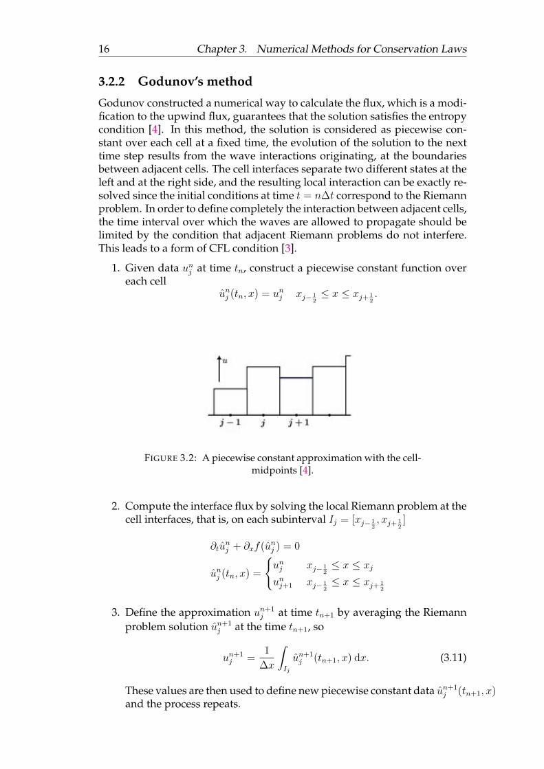
1. Given data unj at time tn, construct a piecewise constant function overeach cell

unj (tn, x) = unj xj− 12≤ x ≤ xj+ 1

2.

FIGURE 3.2: A piecewise constant approximation with the cell-midpoints [4].

2. Compute the interface flux by solving the local Riemann problem at thecell interfaces, that is, on each subinterval Ij = [xj− 1

2, xj+ 1

2]

∂tunj + ∂xf(unj ) = 0

unj (tn, x) =

{unj xj− 1

2≤ x ≤ xj

unj+1 xj− 12≤ x ≤ xj+ 1

2

3. Define the approximation un+1j at time tn+1 by averaging the Riemann

problem solution un+1j at the time tn+1, so

un+1j =

1

∆x

∫Ij

un+1j (tn+1, x) dx. (3.11)

These values are then used to define new piecewise constant data un+1j (tn+1, x)

and the process repeats.


Is conservative scheme with the flux

fj+ 12

=

{minuj≤u≤uj+1

f(uj) uj < uj+1,

maxuj≤u≤uj+1f(uj) uj ≥ uj+1,

(3.12)

which is called the Godunov scheme, (see [5]). Note that this is equal withthe first-order upwind scheme for linear advection equations.

Theorem 3. Godunov scheme is first order consistent with the original prob-lem.

Advantage of Godunov scheme

• Gives the exact solution for the Riemann problem and is valid for anyscaler conservation laws with convex or concave flux.

• Gives the correct flux corresponding to the weak solution satisfying en-tropy condition. More in general, provided we assume the CFL condi-tion.

• Can deal the discontinuity without oscillation.

Remark 2. The solution is exact for short times; in fact its valid until thewaves generated from the solution of Riemann problem start interacting withthe waves generated by the neighboring interfaces, which is due to the par-ticular form of the solution of Riemann problem. i.e. although the generalsolution of the equations is a function of x and t, the solution to the Riemannproblem can be expressed as a function of a single variable namely x/t. Thisproperty is known as similarity [5].

The CFL condition

In order to have stability when using explicit numerical schemes, we are re-quired to apply the necessary condition known as the Courant–Friedrichs–Lewy condition. It is often referred to as the CFL which is:∣∣∣∣∂f∂u ∆t

∆x

∣∣∣∣ ≤ 1

19

Chapter 4

Higher order and TVD methods

The main difficulty in the construction of any high-order method is the reso-lution of two contradictory requirements namely high-order of accuracy andabsence of spurious oscillations.The high-order linear schemes, which are schemes with second or higher or-der spatial accuracy in smooth parts of the solution and also around shocksand discontinuities (see [6] and [3]), produce unphysical oscillations, on theother hand, the class of monotone methods do not produce unphysical oscil-lations. However, monotone methods are at most first order accurate and aretherefore of limited use.One way of resolving the contradiction between linear schemes of high-orderof accuracy and absence of spurious oscillations is by constructing non-linearmethods.

In the following we will state a natural idea to build a non-linear schemein order to have the high order accuracy and avoid oscillation.

4.1 MUSCL- higher order methods

We follow in this section the presentation of in [3] and [6].Godunov gave the basic idea of the one-order conservative schemes whichdeal the oscillations, to achieve higher order of accuracy, van Leer introducedthe idea of modifying the first step of Godunov’s method.This approach has become known as the Monotone Upstream-centered Schemefor Conservation Laws " MUSCL" or Variable Extrapolation approach. TheMUSCL approach allows the construction of very high order methods, fullydiscrete, semi–discrete and also implicit methods.Back to the Godunov’s method which depends on three steps:

• Construct constant data over each cell.

• Solve Riemann problem with this data.

• Take the solution as the cell average.

The first step can be modified without influencing the physical input. VanLeer’s method is based on modifying Godunov scheme in the following way.

20 Chapter 4. Higher order and TVD methods

Steps of van Leer’s methodVan Leer’s method is a second-order slope limiter method which is based onthe concept of non linear discretizations leads to a non linear scheme evenwhen applied to linear equation under the form of limiters, which controlsthe gradient of the computed solution.There are three main steps in the van Leer’s scheme:

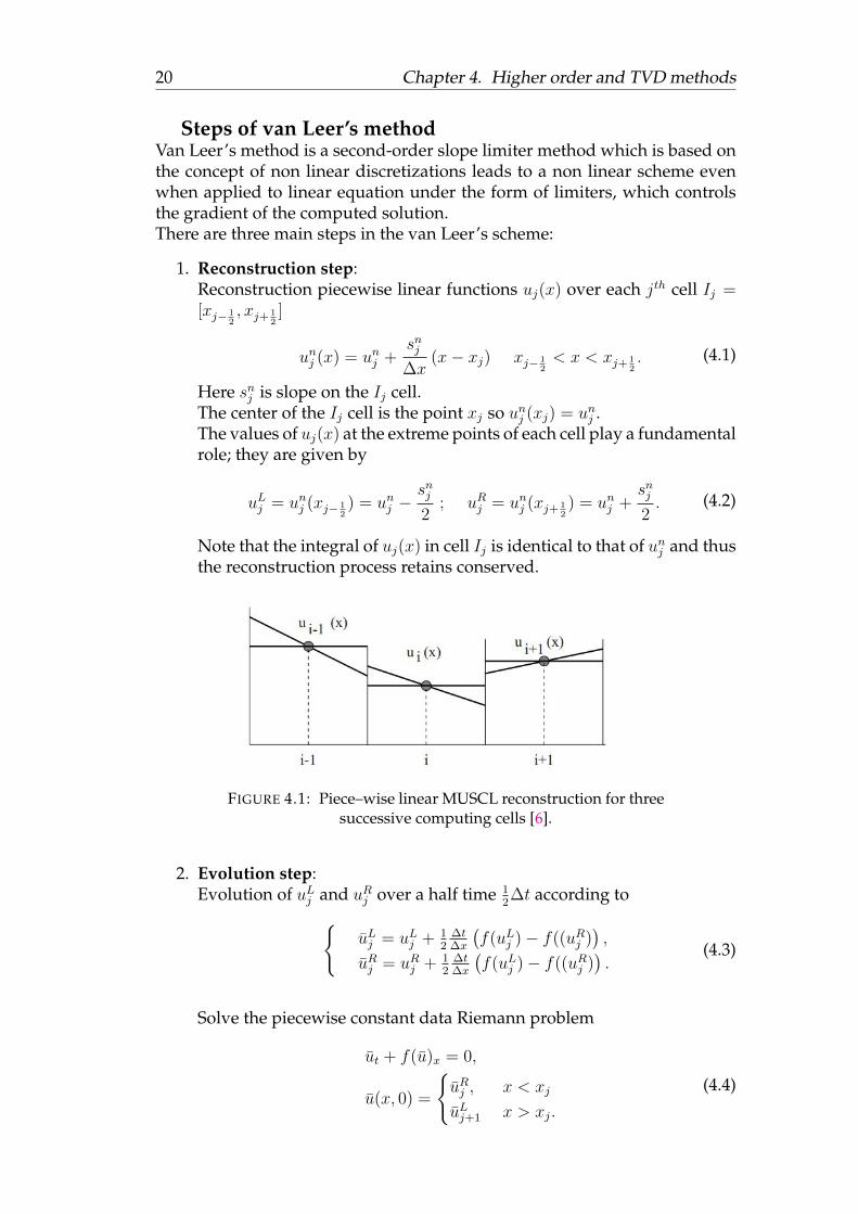
1. Reconstruction step:Reconstruction piecewise linear functions uj(x) over each jth cell Ij =[xj− 1

2, xj+ 1

2]

unj (x) = unj +snj∆x

(x− xj) xj− 12< x < xj+ 1

2. (4.1)

Here snj is slope on the Ij cell.The center of the Ij cell is the point xj so unj (xj) = unj .The values of uj(x) at the extreme points of each cell play a fundamentalrole; they are given by

uLj = unj (xj− 12) = unj −

snj2

; uRj = unj (xj+ 12) = unj +

snj2. (4.2)

Note that the integral of uj(x) in cell Ij is identical to that of unj and thusthe reconstruction process retains conserved.

FIGURE 4.1: Piece–wise linear MUSCL reconstruction for threesuccessive computing cells [6].

2. Evolution step:Evolution of uLj and uRj over a half time 1

2∆t according to{

uLj = uLj + 12

∆t∆x

(f(uLj )− f((uRj )

),

uRj = uRj + 12

∆t∆x

(f(uLj )− f((uRj )

).

(4.3)

Solve the piecewise constant data Riemann problem

ut + f(u)x = 0,

u(x, 0) =

{uRj , x < xj

uLj+1 x > xj.

(4.4)

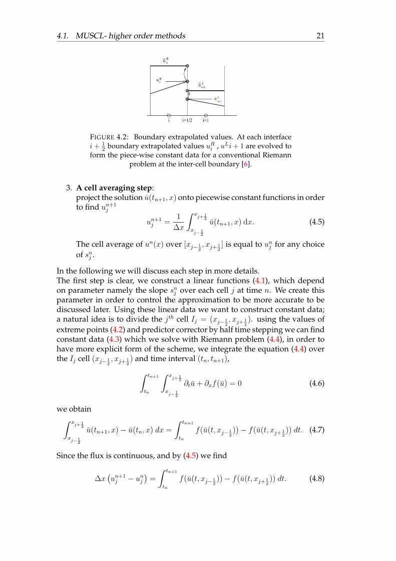
4.1. MUSCL- higher order methods 21

FIGURE 4.2: Boundary extrapolated values. At each interfacei + 1

2 boundary extrapolated values uRi , uLi + 1 are evolved toform the piece-wise constant data for a conventional Riemann

problem at the inter-cell boundary [6].

3. A cell averaging step:project the solution u(tn+1, x) onto piecewise constant functions in orderto find un+1

j

un+1j =

1

∆x

∫ xj+1

2

xj− 1

2

u(tn+1, x) dx. (4.5)

The cell average of un(x) over [xj− 12, xj+ 1

2] is equal to unj for any choice

of snj .

In the following we will discuss each step in more details.The first step is clear, we construct a linear functions (4.1), which dependon parameter namely the slope snj over each cell j at time n. We create thisparameter in order to control the approximation to be more accurate to bediscussed later. Using these linear data we want to construct constant data;a natural idea is to divide the jth cell Ij = (xj− 1

2, xj+ 1

2). using the values of

extreme points (4.2) and predictor corrector by half time stepping we can findconstant data (4.3) which we solve with Riemann problem (4.4), in order tohave more explicit form of the scheme, we integrate the equation (4.4) overthe Ij cell (xj− 1

2, xj+ 1

2) and time interval (tn, tn+1),∫ tn+1

tn

∫ xj+1

2

xj− 1

2

∂tu+ ∂xf(u) = 0 (4.6)

we obtain∫ xj+1

2

xj− 1

2

u(tn+1, x)− u(tn, x) dx =

∫ tn+1

tn

f(u(t, xj− 12))− f(u(t, xj+ 1

2)) dt. (4.7)

Since the flux is continuous, and by (4.5) we find

∆x(un+1j − unj

)=

∫ tn+1

tn

f(u(t, xj− 12))− f(u(t, xj+ 1

2)) dt. (4.8)


The idea here is to approximate the flux, we assume that the numerical fluxis

fnj− 1

2=

1

∆t

∫ tn+1

tn

f(u(t, xj+ 12)) dt. (4.9)

The equation (4.8) becomes

un+1j = unj +

∆t

∆x

[fnj+ 1

2− fn

j− 12

]. (4.10)

Using the midpoint rule, we find

1

∆t

∫ tn+1

tn

f(u(t, xj− 12)) = f(u(tn +

∆t

2, xj+ 1

2)) +O(∆t2). (4.11)

To approximate the numerical flux f we have to approximate f(u(tn+∆t2, xj+ 1

2))

in each cell.Then, we solve the Riemann problem at the point xj+ 1

2with piecewise con-

stant initial data.After solving Riemann problem we have to find the proper slope for eachcell. For better understanding the way of calculating the slope we will studythis method for advection equation.

4.1.1 Van Leer’s method for advection and Burger’s equa-tions

Van Leer’s method for advection equation

Let us consider the following advection equation

ut + cux = 0, c > 0. (4.12)

with nonlinear initial condition and boundary condition.Step I: Gives the boundary extrapolated values (4.2).Step II: we need the fluxes f(uLj ) and f(uRj ). As for the linear advection equa-tion f(u) = cu, then we have

f(uLj ) = c

(unj −

snj2

); f(uRj ) = c

(unj +

snj2

)(4.13)

Then

f(uLj )− f(uRj ) = c

(unj −

snj2− unj −

snj2

)= −csnj (4.14)

Substitute of these into the equation (4.3) gives the evolved boundary extrap-olated values in Ij cell, [6]

uLj = unj −1

2(1 +R) snj

uRj = unj +1

2(1−R) snj

(4.15)


We solve the conventional Riemann problem at the interface j + 12

with data(uRj , u

Lj ) the solution of which is

un+1j+ 1

2

=

{uRj = unj + 1

2(1−R) snj x < c∆t,

uLj+1 = unj+1 − 12

(1 +R) snj+1 x > c∆t(4.16)

Remark 3. We can check easily that by choosing the slope to be sj = uj+1−ujthen van Leer’s method is identical to Lax-Wendroff method.

The above remark affirms that the choice of the slope sj play a main rolefor avoiding the oscillation.

Van Leer method for Burgers’s equation

We solve numerically the following Burgers’s equation with non-linear initialcondition

∂tu(t, x) + u(t, x)∂xu(t, x) = 0 (4.17)

From the equation (4.3) we find{uLj = uLj + 1

4∆t∆x

((uLj )2 − ((uRj )2

),

uRj = uRj + 14

∆t∆x

((uLj )2 − ((uRj )2

). uLj = unj −

snj2

+ 14

∆t∆x

((unj −

snj2

)2 − (unj +snj2

)2),

uRj = unj +snj2

+ 14

∆t∆x

((unj −

snj2

)2 − (unj +snj2

)2).{

uLj = unj −snj2

+ 12

∆t∆x

(snj u

nj

),

uRj = unj +snj2

+ 12

∆t∆x

(snj u

nj

).{

uLj =(1 + ∆t

2∆xsnj)unj −

snj2,

uRj =(1 + ∆t

2∆xsnj)unj +

snj2.

We solve Riemann problem with the following condition{uLj+1 =

(1 + ∆t

2∆xsnj+1

)unj+1 −

snj+1

2,

uRj =(1 + ∆t

2∆xsnj)unj +

snj2,

and take the solution as cell average.


Among the schemes which are free of numerical oscillations is the To-tal Variation Diminishing TVD scheme which is free of oscillation wheneverstability is assured.

Definition 3. A numerical method to solve hyperbolic conservation laws iscalled total variation diminishing if

TV (un+1) ≤ TV (un).

In other words,∞∑−∞

|un+1j+1 − un+1

j | ≤∞∑−∞

|unj+1 − unj |.

we want to choose the slope snj in such way that the scheme becomes aTVD scheme.

Theorem 4. Suppose uj is generated by a numerical method in conservationform with a Lipschitz continuous numerical flux, consistent with some scalarconservation law. If the method is TV -stable, i.e., TV (un) =

∑∞−∞ |unj+1 − unj |

is uniformly bounded for all the approximations at different time; ∀n, j withj < j0, nj ≤ T , then the method is convergent, where T is the final time, (forproof see [2]).

4.1.2 Slope Limiter

We define the slope with the following function

snj = (unj+1 − unj )φnj . (4.18)

Here φnj = φ(rnj ) is a function of rnj which represents the ratio of consecutivegradients

rnj =unj − unj−1

unj+1 − unj, (4.19)

while φ is limiter function defined to obtain a TVD method.We set the following conditions which are sufficient to obtain TVD scheme,

φ(r) = 0 r ≤ 0,

0 ≤ φ(r) ≤ 2r.

To obtain second order accuracy, additional conditions are to be imposed, forexample,

φ(1) = 1.

Remark 4. We can observe thatIf φj = φj−1 = 1 ⇒ Lax–Wendroff (not TVD).If φj = φj−1 = 0 ⇒ Upwind (TVD).

Various limiter functions have been defined in the literature. Actually, weconsider three limiter functions [3] :


Van Leer’s limiter

φ(r) =|r|+ r

1 + |r|. (4.20)

In this case we might write the slope as follows

snj = (unj+1 − unj )|rnj |+ rnj1 + |rnj |

= (unj+1 − unj )|u

nj −unj−1

unj+1−unj|+ unj −unj−1

unj+1−unj

1 + |unj −unj−1

unj+1−unj|

• First case : unj−1 < unj < unj+1 or unj−1 > unj > unj+1

snj = 2(unj+1 − unj )(unj − unj−1)

unj+1 − unj−1

. (4.21)

• Second case : unj−1 < unj and unj > unj+1 or unj−1 > unj and unj < unj+1

Snj = 0. (4.22)

Minmod limiter

Minmod limiter that represents the lowest boundary of the second-orderTVD region:

φ(r) =

{min(r, 1) r > 0

0 r ≤ 0.(4.23)

It is a particular case of the minmod function, defined as the function thatselects the number with the smallest modulus from a series of numbers whenthey all have the same sign, and zero otherwise. For two arguments:

minmod (x, y) =

x |x| < |y|, xy > 0,

y |x| > |y|, xy > 0,

0 xy < 0.

(4.24)

Superbee limiter

The superbee limiter, that represents the upper limit of the second-order TVDregion and has been introduced by Roe:

φ(r) = max[0,min(2r, 1),min(r, 2)]. (4.25)

These three limiters produce second order scheme when the solution is smooth,and reduce to upwind at the discontinuity.


FIGURE 4.3: Popular choices for limiter function [4].

Remark 5. These three limiters possess the following property

φ(r)

r= φ(

1

r).

This property ensures that the top corner of a discontinuity is related sym-metrically to a bottom corner [4].

27

Chapter 5

Numerical Result

In this chapter we will see some results of different numerical methods forconservation laws, using Matlab.

Example 5.0.1. Consider the Burgers equation with discontinuous initial conditionand boundary condition,

ut + (u2

2)x = 0 x ∈ (−1, 2), t ∈ (0, 2)

u(t,−1) = 1 t ∈ (0, 2)

u(t, 2) = 0 t ∈ (0, 2)

u(0, x) =

{1 if − 1 ≤ x < 0 ,

0 if 0 ≤ x ≤ 2.

The following numerical result clearly shows that the Lax–Wendroff’s method oscil-lates at the discontinuity, where Godunov’s method does not oscillate.

Error =0.0358 Error=0.1069

Lax–Wendroff and Godunov’s methods for ∆x = 0.1, ∆t = 0.04and t = 2.

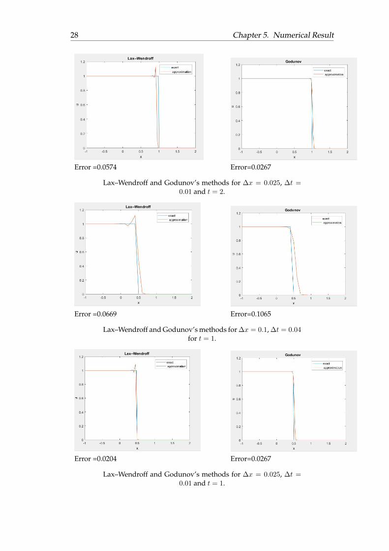
28 Chapter 5. Numerical Result

Error =0.0574 Error=0.0267

Lax–Wendroff and Godunov’s methods for ∆x = 0.025, ∆t =0.01 and t = 2.

Error =0.0669 Error=0.1065

Lax–Wendroff and Godunov’s methods for ∆x = 0.1, ∆t = 0.04for t = 1.

Error =0.0204 Error=0.0267

Lax–Wendroff and Godunov’s methods for ∆x = 0.025, ∆t =0.01 and t = 1.

Chapter 5. Numerical Result 29

Example 5.0.2. Shock wavesWe consider Burgers equation with the following initial condition

ut + (u2

2)x = 0 x ∈ (−1, 2), t ∈ (0, T )

u(t,−1) = 1 t ∈ (0, T )

u(t, 2) = 0 t ∈ (0, T )

u(0, x) =

1 x ≤ 0

1− x 0 ≤ x ≤ 1

0 x ≥ 1

The exact solution for this problem is:

u(t, x) =

1 x ≤ t1−x1−t t ≤ x ≤ 1

0 x ≥ 1

t < 1,

{1 x < s(t)

0 x > s(t).t≥ 1

Here s is the speed s(t) = 1+t2

.The following numerical result clearly shows that the Lax–Wendroff’s method is sec-ond order of accuracy on the smooth solutions, where Godunov’s method is first orderof accuracy.

Error =0.0128 Error=0.0317

Lax–Wendroff and Godunov’s methods for ∆x = 0.1, ∆t = 0.05and t = 0.5.


Error =0.0056 Error=0.0162

Lax–Wendroff and Godunov’s methods for ∆x = 0.05, ∆t =0.025 and t = 0.5.

Error= 0.0027 Error=0.0083

Lax–Wendroff and Godunov’s methods for ∆x = 0.025, ∆t =0.0125 and t = 0.5.

Chapter 5. Numerical Result 31

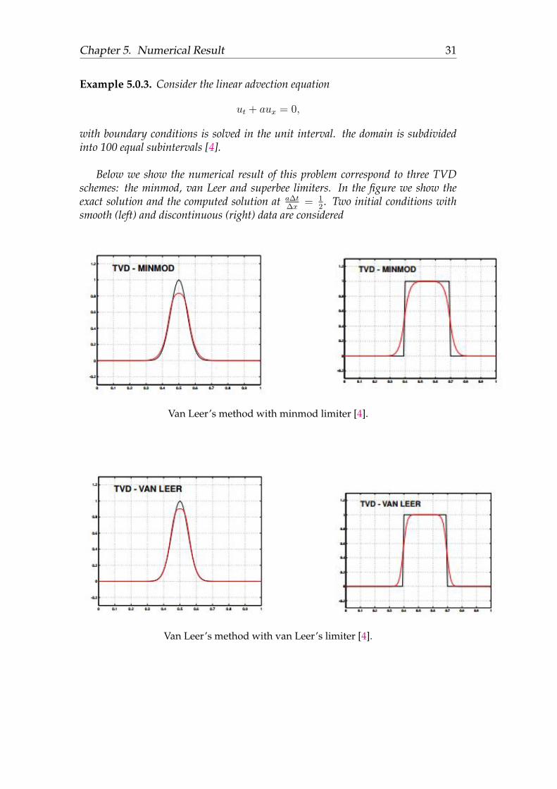
Example 5.0.3. Consider the linear advection equation

ut + aux = 0,

with boundary conditions is solved in the unit interval. the domain is subdividedinto 100 equal subintervals [4].

Below we show the numerical result of this problem correspond to three TVDschemes: the minmod, van Leer and superbee limiters. In the figure we show theexact solution and the computed solution at a∆t

∆x= 1

2. Two initial conditions with

smooth (left) and discontinuous (right) data are considered

Van Leer’s method with minmod limiter [4].

Van Leer’s method with van Leer’s limiter [4].


Van Leer’s method with superbee limiter [4].

33

General Conclusion

conclusion:

In this work, we have studied and simulated the solution of conservationlaws, with three schemes with continuous and discontinuous initial condi-tions. The results show that the Lax–Wendroff’s scheme oscillates at the dis-continuity (not TVD scheme), even if it is second order accurate, differentlythan Godunov scheme which is first order of accuracy but a TVD scheme.The third scheme was van Leer’s scheme, where we have found that thisscheme depends on the choice of the slope. For this, We defined slope func-tions, and stated three popular slope limiters: minmod, van Leer and super-bee, which make the scheme to be TVD and second order of accuracy.

Recommendations for future research:

Through this research experience with the topic of conservation laws, wehave encountered some points that we found interesting and worth more in-vestigation. We ambition to extend our work to if time allows.It would be interesting to study the multi-dimensional extension of the pre-sented methods and the extension to systems. Practically, the computationalefficiency is the most important question. If the slope limiters increase thecomputational costs and the complexity of the computation, would it not bebetter to try an implicit method?.Also, it would be interesting to see how the slope limiters effect the qualita-tive properties of the numerical solution, for example their positivity.

35

Bibliography

[1] Lawrence C. Evans. Partial differential equations, volume 19 of GraduateStudies in Mathematics. American Mathematical Society, Providence, RI,1998. ISBN 0-8218-0772-2.

[2] Randall J. LeVeque. Numerical methods for conservation laws. Lectures inMathematics ETH Zürich. Birkhäuser Verlag, Basel, second edition, 1992.ISBN 3-7643-2723-5. doi: 10.1007/978-3-0348-8629-1. URL http://dx.doi.org/10.1007/978-3-0348-8629-1.

[3] A. Mazzia. Numerical Methods for the solution of Hyperbolic ConservationLaws. Science Applicate, via Belzoni, Italy, 2010.

[4] MIT Massachusetts Institute of Technology. Numerical Schemes forone-dimensional Conservation Laws, Lecture notes 12. 2003. URL https://ocw.mit.edu/courses/aeronautics-and-astronautics/16-920j-numerical-methods-for-partial-differential-equations-sma-5212-spring-2003/lecture-notes/lec12_notes.pdf.

[5] Chi-Wang Shu. Numerical Methods for Hyperbolic Conservation Laws. 2006.

[6] Eleuterio F. Toro. Riemann solvers and numerical methods for fluid dynam-ics. Springer-Verlag, Berlin, third edition, 2009. ISBN 978-3-540-25202-3.doi: 10.1007/b79761. URL http://dx.doi.org/10.1007/b79761.A practical introduction.

http://dx.doi.org/10.1007/978-3-0348-8629-1

http://dx.doi.org/10.1007/978-3-0348-8629-1

https://ocw.mit.edu/courses/aeronautics-and-astronautics/16-920j-numerical-methods-for-partial-differential-equations-sma-5212-spring-2003/lecture-notes/lec12_notes.pdf




http://dx.doi.org/10.1007/b79761

numerical solution of non–linear conservation laws · 2.2. scalar conservation laws 5 (2.5) as...

Documents