7

NASA TECHNICAL NOTE NASA TN D-7865

NUMERICAL SOLUTION OF THE HYPERSONIC

VISCOUS-SHOCK-LAYER EQUATIONS FOR LAMINAR,

TRANSITIONAL, AND TURBULENT FLOWS

OF A PERFECT GAS OVER BLUNT

AXIALLY SYMMETRIC BODIES

E. C. Anderson and James N. Moss

Langley Research Center

Hampton, Va. 23665

MAR 1 71975

Rp' ' i i f i r»i<?*I

NATIONAL A E R O N A U T I C S AND SPACE ADMINISTRATION • WASHINGTON, D. C. • FEBRUARY 1975

https://ntrs.nasa.gov/search.jsp?R=19750008700 2018-08-26T13:01:59+00:00Z

1. Report No.

NASA TN D-78654. Title and Subtitle

NUMERICAL SOLUTION OF 'SHOCK- LAYER EQUATIONSAND TURBULENT FLOWS OlAXIALLY SYMMETRIC BODI

7. Author(s)

E. C. Anderson and James N.

2. Government Accession No.

FHE HYPERSONIC VISCOUS-FOR LAMINAR, TRANSITIONAL.F A PERFECT GAS OVER BLUNTES

Moss

9. Performing Organization Name and Address

NASA Langley Research CenterHampton, Va. 23665

12. Sponsoring Agency Name and Address

National Aeronautics and Space AdministrationWashington, D.C. 20546

3.

5.

6.

8.

10.

11.

13.

14.

Recipient's Catalog No.

Report DateFebruary 1975

Performing Organization Code

Performing Organization Report No.

L-9763Work Unit No.

502-27-03-03Contract or Grant No.

Type of Report and Period Covered

Technical NoteSponsoring Agency Code

15. Supplementary Notes

E . G . Anderson is a research associate with Old Dominion University Research Foundation,• Norfolk, Virginia.

16. Abstract

The viscous-shock-layer equations applicable to hypersonic laminar, transitional, andturbulent flows of a perfect gas over two-dimensional plane or axially symmetric blunt bodiesare presented. The equations are solved by means of an implicit finite-difference scheme,and the results are compared with a turbulent-boundary-layer analysis. The agreementbetween the two solution procedures is satisfactory for the region of flow where streamlineswallowing effects are negligible. For the downstream regions, where streamline swallowingeffects are present, the expected differences in the two solution procedures are evident.

17. Key Words (Suggested by Author(s))

Shock layer, viscousPerfect-gas flowLaminarTurbulent

19. Security Classif. (of this report)

Unclassified

18. Distribution Statement

Unclassified — Unlimited

Subject Category 34Fluid Mechanics and Heat Transfer

20. Security Classif. (of this page)

Unclassified21. No. of Pages

3522. Price*

$3.75

For sale by the National Technical Information Service, Springfield, Virginia 22151

NUMERICAL SOLUTION OF THE HYPERSONIC

VISCOUS-SHOCK-LAYER EQUATIONS FOR LAMINAR, TRANSITIONAL,

AND TURBULENT FLOWS OF A PERFECT GAS OVER

BLUNT AXIALLY SYMMETRIC BODIES

E. C. Anderson* and James N. MossLangley Research Center

SUMMARY

The viscous-shock-layer equations for hypersonic laminar, transitional, and turbu-lent flows of a perfect gas over two-dimensional plane or axially symmetric blunt bodiesare developed and presented. The resulting equations are transformed to a shock-bodyoriented coordinate system and solved by an implicit finite-difference scheme. The eddyviscosity is approximated by a two-layer model which has been used extensively inturbulent-boundary-layer analyses. Methods for defining the boundary-layer-thicknessparameters (required in the eddy-viscosity model) which are consistent with boundary-layer theory are presented.

Numerical solutions of the equations of motion for turbulent viscous shock layersare compared with those of a turbulent-boundary-layer analysis which is not correctedfor the entropy variation of the inviscid flow outside the boundary layer. The two solu-tion procedures are in good agreement in the region of flow where the effects of stream-line swallowing by the boundary layer are negligible. For the downstream regions, wherestreamline swallowing effects are present, the expected differences in the two solutionprocedures are evident. However, to establish the accuracy of the downstream solutions,comparisons with a boundary-layer analysis which accounts for the effects of streamlineswallowing are necessary.

INTRODUCTION

The nose blunting required to reduce the surface heat-transfer rates to an accept-able level in the stagnation region of a hypersonic vehicle results in strong entropy gra-dients through the boundary layer in the downstream region. In the stagnation region,the vorticity interaction between the boundary layer and the external inviscid flow must

Research associate, Old Dominion University Research Foundation, Norfolk,Virginia.

be considered in the analysis if the Reynolds number is sufficiently low. Mayne andAdams (ref. 1) present detailed comparisons of a number of boundary-layer analyses withthe viscous-shock-layer analysis developed by Davis (ref. 2). The results presented byMayne and Adams show that the viscous-shock-layer analysis correctly accounts forviscous-inviscid vorticity interaction, streamline swallowing, and viscous-induced pres-sure effects. Although the viscous-shock-layer analysis was found to be the more accu-rate solution technique, Mayne and Adams demonstrate that a conventional boundary-layeranalysis corrected for streamline swallowing is sufficiently accurate and is computation-ally more efficient than the viscous-shock-layer analysis. The comparisons presentedby Mayne and Adams are restricted to laminar flows of a perfect gas.

As a result of the increased boundary-layer thickness in turbulent flows, the effectsof viscous-induced pressure and the strong entropy gradients produced by the bow shockare more pronounced. For turbulent flows, the solution of the viscous-shock-layer equa-tions should provide a substantially more accurate result than would be obtained with aboundary-layer analysis corrected for streamline swallowing without additional correc-tions to include interaction of the boundary layer with the external inviscid flow.

For flow conditions in which heat transfer from the shock layer by radiation mustbe considered, the formulation of the viscous-shock-layer equations provides an impor-tant simplification. The presence of the radiative heat flux term in both the inviscid andviscous governing equations necessitates an iterative solution procedure of both sets ofequations to achieve the required coupling. Since the necessary coupling of the inviscid-and viscous-flow equations is contained within the viscous-shock-layer equations, thesolution of this set of governing equations should be more accurate and computationallymore efficient than an iterative solution technique which uses a boundary-layer-typeanalysis. However, applications of the viscous-shock-layer equations to turbulent flowshave not been reported. An independent investigation of the viscous-shock-layer equa-tions for turbulent flow has been developed by Eaton and Larson (ref. 3) concurrently withthe present study. The results presented by Eaton and Larson are restricted to the thin-shock-layer assumption and to pointed bodies, as a result of their definition for the loca-tion of the boundary-layer edge. The present study considers the complete viscous-shock-layer equations for turbulent flow and presents definitions for the boundary-layer thicknessand incompressible boundary-layer displacement thickness which are consistent withboundary-layer theory. Both the present study and that of reference 3 are applicable to aperfect gas. Either analysis can, with minor modifications, be applied to equilibriumflows.

It is noted that the boundary-layer-thickness parameters are introduced into thesolution by the two-layer eddy-viscosity model used in the present study and would beunnecessary if an invariant-turbulence model were available. The eddy viscosity isapproximated by use of the formulation proposed by Cebeci (ref. 4).

Numerical solutions of the viscous-shock-layer equations for turbulent flow arecompared with solutions from the boundary-layer analysis developed by Anderson andLewis (ref. 5). The two solution procedures show acceptable agreement over the portionof the body where the effects of streamline swallowing by the boundary layer are negligi-ble, and the expected differences are obtained in the region far downstream of the nose.The boundary -layer analysis does not account for streamline swallowing.

SYMBOLS

A+ damping factor (eqs. (23) and (24))

aQ quantity defined by equation (A9e)

aj quantity defined by equation (AlOf)

&2 quantity defined by equation (AlOg)

Cf skin-friction coefficient

Cp • specific heat at constant pressure

u2

H defined quantity, h + —u

V2Ht total enthalpy, H +

LA

* f * Nh specific enthalpy,

j flow index: 0 for plane flow; 1 for axisymmetric flow

k thermal conductivity

k~, eddy thermal conductivity

H mixing length (eq. (21))

M Mach number

Npr Prandtl number, /j.*cp/k

Npr T turbulent Prandtl number, c^/iit/kit,JL j. y j. ' n x / A

Nfje Reynolds number, P^U^r* m^

* / *n coordinate measured normal to body, n/r

n+ normal coordinate (eq. (22))

P+ pressure-gradient parameter (eq. (25))

p pressure, py p

q* wall heat-transfer rate

* / *r radius measured from axis of symmetry to point on body surface, r /r

r* nose radius

s coordinate measured along body surface, s*/rn

s0 s at beginning of transition

s transition damping factor (eq. (35))

T temperature, T*/T*ef

T* f temperature. (\J*} /c*vpf " \ oo/ / n ooX Cl. \ ^^/ / c )

U^ free-stream velocity

u velocity component tangent-to body surface, u y U ^

u friction velocity (eq. (27))

v velocity component normal to body surface, v^/U^

v+ scaled mean velocity component (eq. (26)), VW/UT

x transition length scale

a shock angle defined in figure 1

a -i jO^^IA ^ \ coefficients in equation (A8)

/3 angle defined in figure 1

y ratio of specific heats

y. normal intermittency factor (eq. (30))

y. t streamwise transition intermittency factor (eq. (34))

6 boundary-layer thickness

<5k incompressible displacement thickness (eq. (29))

e+ normalized eddy viscosity (eq. (4)),

et eddy viscosity, inner law (eq. (20))

€Q eddy viscosity, outer law (eq. (28))

TJ transformed n-coordinate, n/ns

6 body angle defined in figure 1

K body curvature

p. molecular viscosity, p.*/p

p.rj, eddy viscosity (eq. (1))

£ coordinate measured along body surface, | - s

P density of mixture, PyP*

Reynolds number parameter,

1/2M*^)

*U* r*J u I

<p quantity defined by equation (lla)

X vorticity Reynolds number (eq. (33))

X vorticity Reynolds number at beginning of transition

\l> quantity defined by equation (AlOe)

Superscripts:

j .0 for plane flow; 1 for axisymmetric flow

time-averaged quantity

* dimensional quantity

' total differential or fluctuating component

" shock-oriented velocity component (see fig. 1)

Subscripts:

e boundary-layer edge

s shock

w wall

00 free stream

Abbreviations:

BL boundary layer

VSL viscous shock layer

ANALYSIS

Governing Equations

The equations of motion for turbulent viscous shock layers are derived by methods

analogous to those presented by Dorrance (ref. 6) for the turbulent-boundary-layer equa-tions. The resulting equations for the shock-body coordinate system shown in figure 1

are presented in nondimensional form. For turbulent flow, time-averaged quantities are

implied by the nomenclature, and the laminar-flow equations are obtained by neglecting

the turbulent eddy viscosity and eddy thermal conductivity.

The eddy viscosity is expressed in time-averaged fluctuating components as

(1)

and the eddy thermal conductivity is

From the definition of the static turbulent Prandtl number

(3)Krp

and the definition

e+ = ̂ 1 (4)

the governing equations for the flow in laminar or turbulent viscous shock layers can be

expressed as

Continuity:

•^- (r + n cos 9)ipu\ + •%- (1 + n/c)(r + n cos 0 ) ipv \= 0 (5)9s 9n

s-momentum:

3u UVK1 + n/c 3s 3n 1 + n/c 1 + n/c 3s

3p ( j + £+) 3u _ jjwc8n| 8n 1 + n/cl

2« j cos Q+1 + n/c r + n cos

uu/ci

n-momentum:

(6)

p _JL_ »v + v »Z - _Sf£_ + 8E-\1 + n/c 3s 3n 1 + n/c/ 3n (V)

Energy:

\1 + n/c 3s

o3p PU^VK

v — + -3n 1 + n« 3n NPr Npr T/ 3n

; '

r + n cos 0/ Np r l Npr -

State:(8)

. (9)

In these equations, the molecular viscosity as given by Sutherland's law is

n =T +C

(10)

where

Npr

e+Nc ^Pr /^-^- (NPr T -NPr,T V Pr'T

u 8u Mu K3n 1 + n/c

(Ha)

C = - - - (lib)

and

C* = 110.33 K (lie)

The governing equations have a hyperbolic-parabolic nature (ref. 2), the hyperbolicnature arising from the normal-momentum equation. If the thin- shock-layer approxima-tion is made, the normal-momentum equation becomes

When equation (7) is replaced by equation (12), the resulting set of equations is parabolic.Consequently, the equations can be solved by using numerical methods similar to thoseused in solving boundary-layer problems. Equation (12) is used for an initial iteration;then for the final flow-field solution, equation (12) is replaced by equation (7), so that thethin-shock-layer approximation is removed.

Boundary Conditions

Conditions at the body surface.- The no-slip boundary conditions are used in thisstudy. The surface conditions for 77 = 0 are

u = v = 0 (13)

and for this study the temperature and enthalpy at the wall are specified as

Tw = Hw = Constant (14)

Conditions at the shock.- The conditions imposed at the shock are calculated byusing the RankLne-Hugoniot relations. The nondimensional shock relations are as follows:

Mass:

p v" = -sin a (15)S 5

u" = cos a (16)

Momentum:

Ps=^^ + s in 2 *l -J - (17)y M2 V Ps/

Energy:

r o ~ r 2 9sin'2 a + 212yM00

2 sin2 a - (y - 1) || (y -± £L_ (18)

Z 4 o(y " l)(y + 1) M^ sin'2 a

State:

(19)

A transformation is applied to the previous nondimensional viscous-shock-layer

equations and boundary conditions to simplify the numerical computations. The transfor-

mation relations and the transformed equations and boundary conditions are given in theappendix.

Eddy -Viscosity Approximations

A two -layer eddy -viscosity model consisting of an inner law based upon Prandtl's

mixing-length concept and the Clauser-Klebanoff expression (based on refs. 7 and 8) for

the outer law is used in the present investigation. This model, introduced by Cebeci(ref. 4), assumes that the inner law is applicable for the flow from the wall outward to the

location where the eddy viscosity given by the inner law is equal to that of the outer law.The outer law is then assumed applicable for the remainder of the viscous layer. It is

noted that the eddy viscosity degenerates to approximately zero in the inviscid portion ofthe shock layer. The degeneracy is expressed in terms of the normal intermittency fac-

tor given by Klebanoff (ref. 7). The expressions used in the present investigation are

given in the following sections.

Inner-eddy-viscosity approximation.- Prandtl's mixing-length concept is stated in

nondimensional variables as

a2.

"2 9u3n

(20)

10

The mixing length SL is evaluated by using Van Driest's proposal (ref. 9) stated as

4 = (21)

where

-,1/2

'w(22)

Here, kj is the Von Karman constant, which is assumed to have a value of 0.4, and A+

is a damping factor.

Cebeci (ref. 4) suggests that for flows with a pressure gradient, the damping factorbe expressed as

A+ = 26(1 - 11.8P+)'1/2

and for flows with both a pressure gradient and mass injection,

1/2

(23)

A+ = 26 / -v

exp(11.8v+) (24)

where

p+ = -(

P2uT3

(25)

(26)

and

P \anw

1/2

(27)

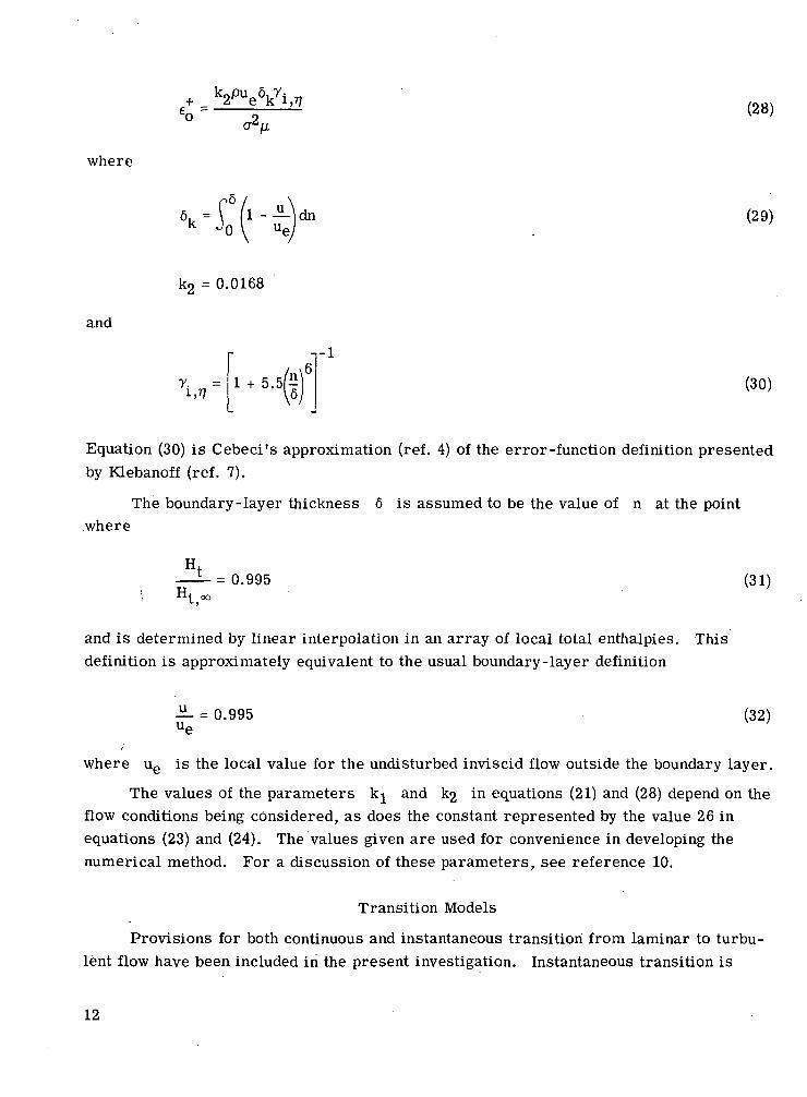
Outer-eddy-viscosity approximation.- For the outer region of the viscous layer theeddy viscosity is approximated by the Clauser-Klebanoff expression

11

where

(28)

p6 / \

= MJ - ~)J udn (29)

and

k2 = 0.0168

5.5/S

-1

(30)

Equation (30) is Cebeci's approximation (ref. 4) of the error-function definition presentedby Klebanoff (ref. 7).

The boundary-layer thickness 6 is assumed to be the value of n at the point.where

H^= 0.995 (31)

and is determined by linear interpolation in an array of local total enthalpies. Thisdefinition is approximately equivalent to the usual boundary-layer definition

u-ii- = 0.995 (32)

where ue is the local value for the undisturbed inviscid flow outside the boundary layer.

The values of the parameters kj and k2 in equations (21) and (28) depend on theflow conditions being considered, as does the constant represented by the value 26 inequations (23) and (24). The values given are used for convenience in developing thenumerical method. For a discussion of these parameters, see reference 10.

Transition Models

Provisions for both continuous and instantaneous transition from laminar to turbu-lent flow have been included in the present investigation. Instantaneous transition is

12

initiated when the local Reynolds number or momentum-thickness Reynolds numberexceeds a preselected value. Continuous transition is effected by defining a streamwisetransition intermittency factor y. ,. which modifies the composite eddy viscosity e+

1 ;S

over an interval x. The factor y. ,. is initially set to zero and is evaluated when the

vorticity Reynolds number (proposed by Rouse, ref. 11, as the stability index)

n o ou /o o \X - — w«*/

exceeds a critical value Xp- For the evaluation of y. ,., the relation1>5

Vj t = 1 - exp(-0.412s) (34)

was used, where

s = 4^"So) (35)

This model was developed by Dhawan and Narasimha (ref. 12) on the basis of the experi-mental data presented by Owen (ref. 13). Approximate values of xc and x are

2000 = xc = 400°

and •

x =2

The values of Xn and x are strongly influenced by the body shape and flow conditionsL-

being considered and are more appropriately defined by comparison with experimentaldata. A discussion of these parameters is given by Harris (ref. 10).

Method of Solution

The procedure for solving the viscous-shock-layer equations is presented herein.First, the finite-difference expressions used to transform the differential equations toalgebraic equations are presented. Then the solution procedure is discussed.

Finite-difference expressions.- The derivatives are converted to finite-differenceform by using Taylor's series expansions. A variable grid spacing (fig. 2) is used in theTj-direction so that the grid spacing can be made small in the region of large gradients.

13

Three-point differences are used in the rj-direction, and two-point, fully implicit differ-ences are used in the ^-direction. Truncation terms of order A£m (first-order accu-racy) and either A?] An, or ATJ - AT? _.. (second-order accuracy) are neglected. A

typical finite-difference expansion of the standard differential equation (see eq. (A8))

gives

Wn-1 + BnWm,n + CnWm>n+1 = Dn (36)

The coefficients A, B, C, and D are used to represent the coefficients after thefinite-difference expansion of equation (A8). The subscript n denotes the grid pointsalong a line normal to the body surface, whereas the subscript m denotes the grid sta-

tions along the body surface. Equation (36) along with the boundary conditions constitutesa system of the tridiagonal form, for which efficient computational procedures are avail-able. (See ref. 14.)

Overall solution procedure.- For specified free-stream conditions and body geom-etry, a stagnation-streamline solution is obtained. With the stagnation-streamline solu-tion providing the initial conditions, the conditions at the shock providing the outer bound-ary conditions, and the conditions at the wall taken as the inner boundary conditions, thenumerical solution is marched downstream to the desired body location £. The firstsolution pass provides only an approximate flow-field solution, because the followingassumptions are used in the first solution pass:

(a) The thin-shock-layer form of the n-momentum equation (eq. (A12b)) is used.

(b) The stagnation-streamline solution is independent of downstream influence(approximation of local similarity where T\% s - 0).

(c) The term dns/d£ is equated to zero at each body station.

(d) The shock angle a is assumed to be the same as the body angle 9.

These assumptions are then removed by making one or more additional solutionpasses. For the current study, a total of two solution passes are used since the twopasses resulted in a converged flow-field solution. For the second solution pass, thethin-shock-layer form of the normal-momentum equation (eq. (A12b)) is replaced by equa-

tion (A12a). The v component of velocity that is used in equation (A12a) is the valuefrom the previous solution pass. Also, once the first solution pass has been computed,the values of n^ s and dng/d£ are calculated and used in the second solution pass toremove approximations (b), (c), and (d). Hence, the viscous-shock-layer equations aresolved as parabolic equations, and yet retain effects which are elliptic and hyperbolic innature. This solution procedure is programed for the Control Data Corporation 6600 com-puter. The execution time is approximately 0.03 second per grid point for a convergedsolution. (This includes all local iterations and solution passes.)

14

Shock solution.- The shock solution procedure at any location is identical for thefirst and subsequent solution passes. However, the shock angle a is defined differentlyfor the first and subsequent solution passes and is set equal to the local body angle 6 forthe first solution pass. For subsequent solution passes, the shock angle is defined as

1a = 6 + tan'1 - - — (37)1 + /ois

Solution procedure at station m.- The viscous-shock-layer equations are solved atany body station m (see fig. 2) in the order shown in figure 3. The governing equationsare uncoupled and the dependent variables are solved one at a time, also in the ordershown in figure 3. First, the shock conditions are calculated to establish the outer bound-ary conditions. Then the converged profiles at station m - 1 are used as the initialguess for the profiles at station m. The solution is then iterated locally until conver-gence is achieved. For the stagnation streamline (m = 1), guess values for the profilesare used to start the solution.

The first-order equations are numerically integrated by means of the trapezoidrule. Each of the second-order partial differential equations is individually integratednumerically by using the tridiagonal formalism (eq. (36)). The global -continuity equa-tion is used to obtain both the shock standoff distance and the v components of velocity.By integrating equation (All) between the limits of TJ = 0 and 77 = 1 at station m, animplicit equation for ns is obtained. For the v component of velocity at TJ, equa-tion (All) is integrated with respect to TJ between the limits of 0 to TJ. The pressure pis determined at station m by integrating the normal- momentum equations (A12) withrespect to TJ between the limits of 1 to TJ. The equation of state is used to determinethe density.

DISCUSSION AND RESULTS

Comparisons are made between the present viscous-shock-layer analysis andturbulent-boundary-layer solutions obtained with the computer program described in ref-erence 15. For the data presented, fully developed turbulent flow without mass injectionhas been assumed. However, provisions have been included for the analysis of continuousor instantaneous transition and for mass injection at the surface.

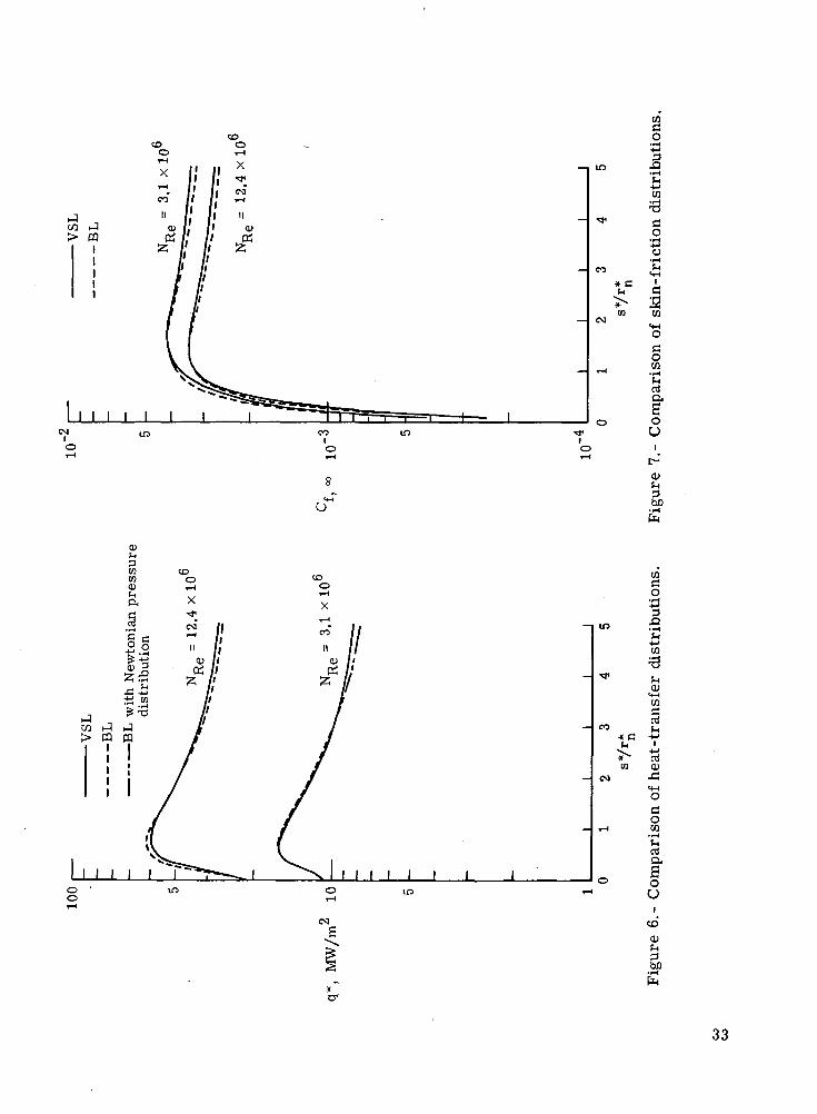
Results are presented for a Mach 19 flow about a 45° (total angle) hyperboloid witha nose radius of 0.3048 meter for free-stream Reynolds numbers of 3.1 x 10^ and12.4 x 10". The wall temperature is taken to be one-tenth of the stagnation temperature,and the free-stream temperature is 256 K. The Prandtl number and the turbulent Prandtlnumber are assumed to be 0.72 and 0.90, respectively.

15

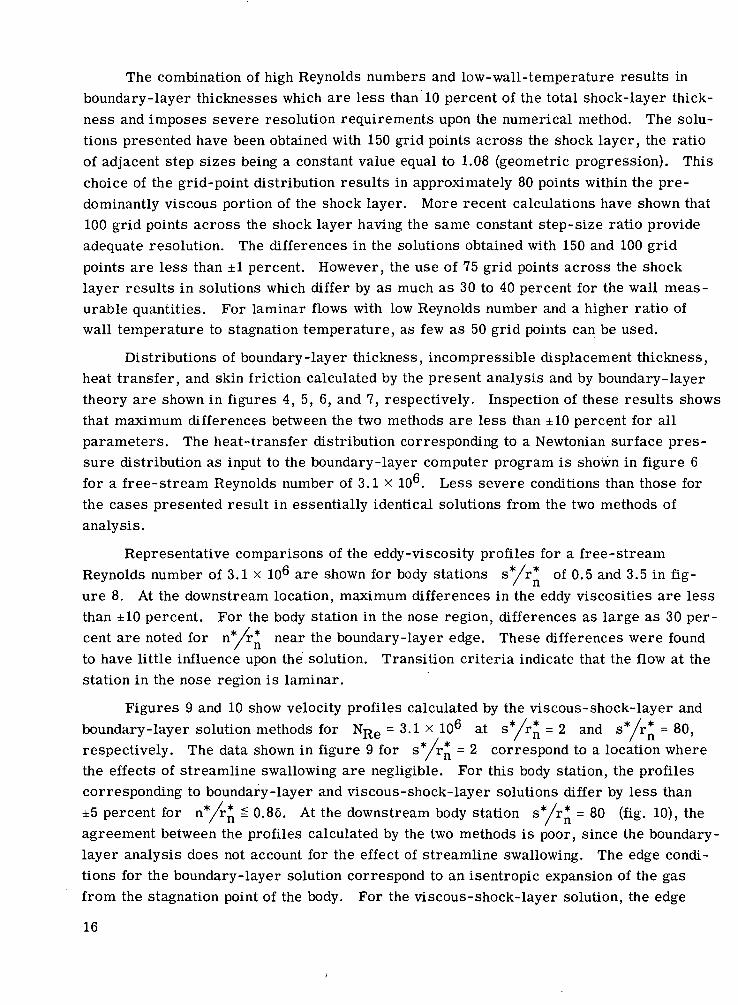
The combination of high Reynolds numbers and low-wall-temperature results inboundary-layer thicknesses which are less than 10 percent of the total shock-layer thick-ness and imposes severe resolution requirements upon the numerical method. The solu-tions presented have been obtained with 150 grid points across the shock layer, the ratioof adjacent step sizes being a constant value equal to 1.08 (geometric progression). Thischoice of the grid-point distribution results in approximately 80 points within the pre-dominantly viscous portion of the shock layer. More recent calculations have shown that100 grid points across the shock layer having the same constant step-size ratio provideadequate resolution. The differences in the solutions obtained with 150 and 100 gridpoints are less than ±1 percent. However, the use of 75 grid points across the shocklayer results in solutions which differ by as much as 30 to 40 percent for the wall meas-urable quantities. For laminar flows with low Reynolds number and a higher ratio ofwall temperature to stagnation temperature, as few as 50 grid points can be used.

Distributions of boundary-layer thickness, incompressible displacement thickness,heat transfer, and skin friction calculated by the present analysis and by boundary-layertheory are shown in figures 4, 5, 6, and 7, respectively. Inspection of these results showsthat maximum differences between the two methods are less than ±10 percent for allparameters. The heat-transfer distribution corresponding to a Newtonian surface pres-sure distribution as input to the boundary-layer computer program is shown in figure 6for a free-stream Reynolds number of 3.1 x 10^. Less severe conditions than those forthe cases presented result in essentially identical solutions from the two methods ofanalysis.

Representative comparisons of the eddy-viscosity profiles for a free-streamReynolds number of 3.1 x 106 are shown for body stations sVr* of 0.5 and 3.5 in fig-ure 8. At the downstream location, maximum differences in the eddy viscosities are lessthan ±10 percent. For the body station in the nose region, differences as large as 30 per-

* / *cent are noted for n /r near the boundary-layer edge. These differences were foundto have little influence upon the solution. Transition criteria indicate that the flow at thestation in the nose region is laminar.

Figures 9 and 10 show velocity profiles calculated by the viscous-shock-layer andboundary-layer solution methods for NRe = 3.1 x 106 at s*/r* = 2 and s*/!•* = 80,respectively. The data shown in figure 9 for s*/r* = 2 correspond to a location wherethe effects of streamline swallowing are negligible. For this body station, the profilescorresponding to boundary-layer and viscous-shock-layer solutions differ by less than±5 percent for n*/r* ^ 0.86. At the downstream body station s*/r* = 80 (fig. 10), theagreement between the profiles calculated by the two methods is poor, since the boundary-layer analysis does not account for the effect of streamline swallowing. The edge condi-tions for the boundary-layer solution correspond to an isentropic expansion of the gasfrom the stagnation point of the body. For the viscous-shock-layer solution, the edge

16

conditions correspond to the flow which crosses the weaker portions of the bow shock,where the entropy jump across the shock is much less than at the stagnation streamline.For the 45° (total angle) hyperboloid considered, the asymptotic limit approaches thesolution for an equivalent cone. For the body station s/'r* = 80, the conditions at theedge of the boundary layer as calculated with the viscous-shock-layer analysis differfrom the cone solution by less than 1 percent. The surface pressure corresponding tothe viscous-shock-layer solution at this station is approximately 15 percent higher thanthe corresponding inviscid cone solution. However, as previously mentioned, in the outerinviscid region the solution is approximately the same as the asymptotic cone solution.The increase in pressure through the predominantly viscous layer was also noted byMayne and Adams (ref. 1) for laminar flow. For laminar flows, the viscous-shock-layersolution used in the present analysis is the same as that used in reference 1. Results forlaminar flows are not presented.

Heat-transfer distributions corresponding to the viscous-shock-layer and boundary-layer solutions for Np^e = 3.1 x 10^ are shown in figure 11. The two solutions show theexpected differences, and the viscous-shock-layer analysis appears to account correctlyfor streamline swallowing. However, the boundary-layer analysis used in the presentstudy does not account for streamline swallowing, and the accuracy of the viscous-shock-layer analysis must be assessed by comparison with an appropriately modified boundary-layer analysis.

For the solution of the turbulent-viscous-shock-layer equations, the use ofKlebanoff's intermittency factor (ref. 7) is essential, whereas in boundary-layer solutions,the intermittency factor may be assumed unity without significantly influencing the resultsobtained. (See ref. 16.) For the viscous-shock-layer equations, the use of a unit inter-mittency factor results in an increase in heat transfer and skin friction of 30 to 50 percentfor s*/r* > 2. This difference in behavior of the viscous-shock-layer and boundary-layer solutions is the result of the nonvanishing tangential velocity gradients in thenormal-coordinate direction. (See fig. 9.) For the boundary-layer equations, the bound-ary conditions imposed ensure that the gradients in the normal-coordinate directionapproach zero at the boundary-layer edge.

CONCLUSIONS

Equations describing the turbulent viscous shock layers over blunt axially symmet-ric bodies of analytic shape are presented for hypersonic flow of a perfect gas. A two-layer eddy-viscosity model consisting of an inner law based upon Prandtl's mixing-lengthconcept and the Clauser-Klebanoff expression for the outer law is used in the presentstudy. Methods for defining the boundary-layer thickness and incompressible boundary-layer displacement thickness which are consistent with boundary-layer theory are pre-

17

sented. An implicit finite-difference technique for solving the equations is given. Com-parisons of the present results with previously reported boundary-layer solutions aremade for a Mach 19 flow over a 45° hyperboloid. The free-stream Reynolds numbersare 3.1 x 10^ and 12.4 x 10^, whereas the wall temperature is one-tenth of the stagnationtemperature.

Results of the study lead to the following conclusions:

1. The present results are in good agreement with classical boundary-layer resultsin regions where the effects of streamline swallowing are negligible. However, for thedownstream locations, where streamline swallowing effects are present, expected differ-ences between the present results and the classical boundary-layer results are evident.

2. For the solution of the turbulent-viscous-shock-layer equations, the use ofKlebanoff's normal intermittency factor is essential. This is in marked contrast withturbulent-boundary-layer solutions, where the normal intermittency factor may beassumed unity without significantly influencing the results.

3. For the flow conditions considered, a boundary-layer thickness (required in theeddy-viscosity model) based on a total-enthalpy ratio provides good agreement withboundary-layer results.

Langley Research Center,National Aeronautics and Space Administration,

Hampton, Va., January 21, 1975.

18

APPENDIX

TRANSFORMED VISCOUS-SHOCK-LAYER EQUATIONS

This appendix presents the transformed viscous-shock-layer equations and boundaryconditions. First, the relations defining the transformed variables and coordinates aregiven. Next, the general equations and boundary conditions are given. Then, the specialform of the equations for the stagnation streamline are developed along with the stagna-tion shock relations.

Transformation Relations

To simplify the numerical computations, a transformation is applied to the viscous-shock-layer equations. This transformation is accomplished by normalizing most of thevariables by their local shock values. When the normal coordinate is normalized withrespect to the local shock standoff distance, a constant number of finite-difference gridpoints between the body and shock are used. This procedure eliminates the need forinterpolation to determine shock shape and the addition of grid points in the normal direc-tion as the computation moves downstream.

The transformed variables are

n

= s

u =u

V -

p =P̂S

-p-^-— TT =-i-

H = J L

Ms

ao =

ai =

a0 =

(Al)

a2,s

where bars over the quantities denote normalization with respect to the shock value. Thetransformations relating the differential quantities are

— = JL § JL8s nc 877

(A2)

19

APPENDIX - Continued

where

dn-

= __ (A4)9n ns 877

and

,29' x u - (A5)9 9 9

9nz ngz 8ryz

The transformations used to express the shock-oriented velocities u" and v" interms of the body-oriented coordinate system (fig. 1) are

us = Ug' sin (a + $) + v£ cos (a + /3) (A6)

and

vq = -u" cos (a + |3) + v" sin (ex + /3) .(A7)° o S

Transformed Equations

After the governing equations are written in transformed variables and coordinates,the second-order partial differential equations are written in the following form:

The quantity W represents u in the s-momentum equation and H in the energy equa-tion. The coefficients a^ to a^ are written as follows:

s-momentum, W = u:

a - 1 850 , ns* L ^ \ [ Jns cos e |

nsPsusns puy nsPsvs pv

1 a0 877 1 + n^K ^ a0)Sa0/ + r + nsr? cos 9 +

CT2a0)S(l + ns77/c) a0 a2a0)S a0

(A9a)

20

APPENDIX - Continued

8ao ns K I K i cos e877 r + n7] cos

upao

n pvao

(A9b)

Qfo = --

PS ns »»?(A9c)

Psusns

where

(A9d)

an = (A9e)

Energy, W = H:

9a! 1 = ~— + ns'-^ +

K ^ j COS 8

3.1 8^] \ 1 + ns7j«; r + ns?7 cos ol,sal

1 +- vspv (AlOa)

H(AlOb)

Q!Q =

al,salHs

cos

1 + ns7]K r + ns7j cos(AlOc)

(AlOd)

21

APPENDIX - Continued

where

2*1 +'rjnaK

a (AlOe)

e+Na1 =s

Pr (AlOf)

1 2" N Pr- 1 , (AlOg)

The preceding energy equation is for the thin-shock-layer approximation. When equa-tion (7). is used for the n-momentum equation, the following term must be added toequation (AlOc):

nsvsv

(AlOh)

The remaining equations are written as follows:

Global continuity:

9 i— ns(r +.n srj cos 0)J/

n-momentum:

cos - 0

(All)

PU*T) / us n£

pu'" +Ps

usnsvs= 0 (A12a)

22

APPENDIX - Continued

which, if the thin-shock-layer approximation is made, becomes

_f_ " /"111

877 p (1 + ns7iK)O

(A12b)

State:

— P = PT (A13)

Equations (A8) to (A13) along with the appropriate boundary conditions are the gov-erning relations used to describe the viscous shock layer for a perfect gas.

Boundary Conditions

Conditions at the body surface.- The surface boundary conditions in terms of trans-formed variables are

u - v = 0 (A14)

Tw = Hw = Constant (A15)

Conditions at the shock. - The shock conditions are determined by solving equa-tions (15) to (19). The transformed shock conditions become

u = T = H=v = p = p = j i I = a Q = ai = a2 = l (A16)

at 77 = 1.

Stagnation-Streamline Equations

When downstream numerical solutions are required, it is necessary to have anaccurate solution for the flow along the stagnation streamline. A truncated series, whichhas the same form as that used by Kao in reference 17, is used to develop the stagnation-streamline equations. The flow is assumed to be laminar along the stagnation streamline.The flow variables are expanded about the axis of symmetry with respect to the nondimen-sional distance | along the body as follows:

+ . . . (A17a)

23

APPENDIX - Continued

. . . (A17b)

= VI(TJ) + . . . (A17c)

. • • (A17d)

. . . • (A17e)

. . . (A17f)

The shock standoff distance is written as

Furthermore, | is small and the curvature K is approximately 1 in the stagnationregion. Consequently, the geometric relations (see fig. 1), including terms of order £,can be written as

/3 * £ (A19)

and

(A20)

Therefore,

sin (a + /3) * 1 (A21)

and

2n2 |cos (a + 0) * —^— (A22)

1 + nl,s

24

APPENDIX - Continued

The shock relations (eqs. (15) to (19)) in terms of expanded variables become

1'l.s

- 1) + 2

+ 1)(A23)

us = (A24)

PS =

and

i,s/

(A25)

(A26)

An examination of these equations shows that the equations for us and p con-tain n9 . This term cannot be determined from the stagnation solutions, since it is a

6,isfunction of the downstream flow. Consequently, a value must be assumed for n^ g. Inthis study, it is assumed to be zero to start the solution, but this assumption is thenremoved by iterating on the solution with the previous shock standoff distances used todefine ^ §• ^ne effect of the downstream shock shape on the stagnation-point solutionis elliptic rather than parabolic.

Along the stagnation streamline, the second-order differential equations are writtenas

(A27)d,The coefficients are defined as

s-momentum, W = u:

= "1 SP1 SV1 Si,s i,s i,s (A28a)

L,S

25

APPENDIX - Continued

l,s^77

"1;S . pl.snl.su]

-2Pl.snl.s

L,s

(A28b)

(A28c)

Energy (enthalpy), W = H:

Npr>1

Q!o = 0

(A29b)

(A29c)

The preceding energy equation is for the thin-shock-layer approximation. When equa-tion (7) is used for the n-momentum equation, the following term must be added to equa-tion (A29c):

nl,svl,sPl,s(NPr,l)s NPr,

Mi dr?

The remaining equations are written as follows:

Global continuity:

d J+1, = -(j + 1)11, (1 + n, 77)^1 _u, p.u. (A30)i,t>\ J.,a l J.,o i,o J. J.

26

APPENDIX - Concluded

n- momentum:

! (A31a)

dry

When the thin- shock-layer approximation is made, the n-momentum equation becomes

5l = 0 (A31b)d?]

The iL term that appears in equation (A28c) can be expressed as

dP2 _ pl.sul.snl,s ^Iai2 2pl,sul,sn2,svl,s *W ^1^2^1,5^,5-- ^1" + V

dr? PI)S l + ̂ ?n1)S p1>s l + r?n1;Sdr? p2 ^ dn

(A31c)

For the thin-shock-layer approximation, this term is

2 - - 2dp9 PT u* n, p^u ,_2= l,s l,s l,s - 1_1 - (A31d)

dr? p l jg l

These equations along with the equation of state constitute the nonlinear ordinary differ-ential equations that are solved along the stagnation streamline.

27

REFERENCES

1. Mayne, A. W., Jr.; and Adams, J. C., Jr.: Streamline Swallowing by Laminar Bound-ary Layers in Hypersonic Flow. AEDC-TR-71-32, U.S. Air Force, Mar. 1971.(Available from DDC as AD 719 749.)

2. Davis, R. T.: Numerical Solution of the Hypersonic Viscous Shock-Layer Equations.AIAA J., vol. 8, no. 5, May 1970, pp. 843-851.

3. Eaton, R. R.; and Larson, D. E.: Laminar and Turbulent Viscous Shock Layer Flowin the Symmetry Planes of Bodies at Angle of Attack. AIAA Paper No. 74-599,June 1974.

4. Cebeci, Tuncer: Behavior of Turbulent Flow Near a Porous Wall With PressureGradient. AIAA J., vol. 8, no. 12, Dec. 1970, pp. 2152-2156.

5. Anderson, E. C.; and Lewis, C. H.: Laminar or Turbulent Boundary-Layer Flows ofPerfect Gases or Reacting Gas Mixtures in Chemical Equilibrium. NASA CR-1893,1971.

6. Dorrance, William H.: Viscous Hypersonic Flow. McGraw-Hill Book Co., Inc.,c.1962.

7. Klebanoff, P. S.: Characteristics of Turbulence in a Boundary Layer With ZeroPressure Gradient. NACA Rep. 1247, 1955. (Supersedes NACA TN 3178.)

8. Clauser, Francis H.: The Turbulent Boundary Layer. Vol. IV of Advances in AppliedMechanics, H. L. Dryden and Th. von Karman, eds., Academic Press, Inc., 1956,pp. 1-51.

9. Van Driest, E. R.: On Turbulent Flow Near a Wall. J. Aeronaut. Sci., vol. 23, no. 11,Nov. 1956, pp. 1007-1011, 1036.

10. Harris, Julius E.: Numerical Solutions of the Equations for Compressible Laminar,Transitional, and Turbulent Boundary Layers and Comparisons With ExperimentalData. NASA TR R-368, 1971.

11. Rouse, Hunter: A General Stability Index for Flow Near Plane Boundaries. J.Aeronaut. Sci., vol. 12, no. 4, Oct. 1945, pp. 423-431.

12. Dhawan, S.; and Narasimha, R.: Some Properties of Boundary Layer Flow During theTransition From Laminar to Turbulent Motion. J. Fluid Mech., vol. 3, pt. 4, Jan.1958, pp. 418-436.

13. Owen, F. K.: Transition Experiments on a Flat Plate at Subsonic and SupersonicSpeeds. AIAA J., vol. 8, no. 3, Mar. 1970, pp. 518-523.

14. Conte, S. D.: Elementary Numerical Analysis. McGraw-Hill Book Co., Inc., c.1965.

28

15. Miner, E. W.; Anderson, E. C.; and Lewis, Clark H.: A Computer Program for Two-Dimensional and Axisymmetric Nonreacting Perfect Gas and Equilibrium Chemi-cally Reacting Laminar, Transitional, and/or Turbulent Boundary Layer Flows.VPI-E-71-8, May 1971. (Available as NASA CR-132601.)

16. Lewis, Clark H.; Miner, E. W.; and Anderson, E. C.: Effects of Strong Axial Pres-sure Gradients on Turbulent Boundary-Layer Flows. Turbulent Shear Flows,AGARD-CP-93, Jan. 1972, pp. 21-1 - 21-14.

17. Kao, Hsiao C.: Hypersonic Viscous Flow Near the Stagnation Streamline of a BluntBody: I. A Test of Local Similarity. AIAA J., vol. 2, no. 11, Nov. 1964,pp. 1892-1897,

29

00

SHOCK

1/K*

30

Shock solution at station m

Initial guess for all profile quantities

1Solve equations (A8) and (A10) for H

Solve equation (A13) for p

Solve equations (A8) and (A9) for u

Solve equations (All) for n and vs

Solve equations (A12) for p

Solve equation (A13) for p

No

Transport properties

Advance to stationm + 1

Figure 3.- Flow chart for solution sequence of viscous-shock-layer equations.

31

If-l

1 a§ s•° 2*-• -2o "Cs «O -Hco -3

8o

0)!H

COCOo>

*c'«

32

CO iJ> CQ

(M

O

* c

co

o

4O>

CO;-.PCOCO<utnD,

S

'« r;

-2.2I-B^5J3£S 2•̂ "̂?T3

J ijCQ CQ

1

1

1

CD0i-H

X

"*.ci*— t

IIcuts

^

If

/

/

f|

;/';/

coo

*C

I I I I Ioo

CO

o

1.pHS-i

-4->

CO

aoo'CIcCO

floCO

'fnrtQ.aoo

c-o>

bD

CO

o

^-t_JCO

CO

o>

oCO-nrta.So

ICO

OJ

bJ)

33

> m

* dSH

X

* 8

COcu

O

O.

>>-M*rHCOOOCO

"g

CO

§CO

aSO

co01S-i

3,

34

1.0 .-

U

BL

I I1.0 2.0

-X VSL

Shock location

3.0 4.0

Figure 10.- Comparison of tangential velocity profiles at syr* = 80. NRg = 3.1 x

q*, MW/m

VSL

BL

J I I J I0 20 40 60 80 100 120 140

s*/r*

Figure 11.- Comparison of heat-transfer distributions. NRe = 3.1 x 106.

NASA-Langley, 1975 L-9763 35

NATIONAL AERONAUTICS AND SPACE ADMINISTRATION

WASHINGTON. D.C. 2O546

OFFICIAL BUSINESS

PENALTY FOR PRIVATE USE $3OO SPECIAL FOURTH-CLASS RATEBOOK

POSTAGE AND FEES PAID

NATIONAL AERONAUTICS AND

SPACE ADMINISTRATION

451

2PHILCO FORD COBP

TciS5SoBIClTIOIS OPERATIONSTECHNICAL INFO SERVICES

JAMBOREE & FORD BOADSBEACH CA 92663

POSTMASTER : If Undeliverable (Section 158Postal Manual) Do Not Return

"The aeronautical and space activities of the United States shall beconducted so as to contribute . . . to the expansion of human knowl-edge of phenomena in the atmosphere and space. The Administrationshall provide for the widest practicable and appropriate disseminationof information concerning its activities and the results thereof."

—NATIONAL AERONAUTICS AND SPACE ACT OF 1958

NASA SCIENTIFIC AND TECHNICAL PUBLICATIONSTECHNICAL REPORTS: Scientific andtechnical infotmation considered important,complete, and a lasting contribution to existingknowledge.

TECHNICAL NOTES: Information less broadin scope but nevertheless of importance as acontribution to existing knowledge.

TECHNICAL MEMORANDUMS:Information receiving limited distributionbecause of preliminary data, security classifica-tion, or other reasons. Also includes conferenceproceedings with either limited or unlimiteddistribution.

CONTRACTOR REPORTS: Scientific andtechnical information generated under a NASAcontract or grant and considered an importantcontribution to existing knowledge.

TECHNICAL TRANSLATIONS: Informationpublished in a foreign language consideredto merit NASA distribution in English.

SPECIAL PUBLICATIONS: Informationderived from or of value to NASA activities.Publications include final reports of majorprojects, monographs, data compilations,handbooks, sourcebooks, and specialbibliographies.

TECHNOLOGY UTILIZATIONPUBLICATIONS: Information on technologyused by NASA that may be of particularinterest in commercial and other non-aerospaceapplications. Publications include Tech Briefs,Technology Utilization Reports andTechnology Surveys.

Details on the availability of these publications may be obtained from:

SCIENTIFIC AND TECHNICAL INFORMATION OFFICE

N A T I O N A L A E R O N A U T I C S A N D S P A C E A D M I N I S T R A T I O N

Washington, D.C. 20546