numerical treatment of coupled nonlinear hyperbolic … · 3 numerical treatment of coupled...
TRANSCRIPT
NUMERICAL TREATMENT OF COUPLED NONLINEAR HYPERBOLICKLEIN-GORDON EQUATIONS
E.H. DOHA1,a, A.H. BHRAWY2,3,b, D. BALEANU4,5,6,c, M.A. ABDELKAWY3,d
1Department of Mathematics, Faculty of Science, Cairo University, Giza, Egypt,E-maila: [email protected]
2Department of Mathematics, Faculty of Science, King Abdulaziz University,Jeddah 21589, Saudi Arabia,
E-mailb: [email protected] of Mathematics, Faculty of Science, Beni-Suef University,
Beni-Suef 62511, Egypt,E-maild: [email protected]
4Department of Chemical and Materials Engineering, Faculty of Engineering,King Abdulaziz University, Jeddah 21589, Saudi Arabia
5Department of Mathematics and Computer Sciences, Cankaya University,Eskisehir Yolu 29.km, 06810 Ankara, Turkey
6Institute of Space Sciences, P.O. BOX, MG-23, RO 077125, Magurele-Bucharest, Romania,E-mailc: [email protected]
Received October 10, 2013
A semi-analytical solution based on a Jacobi-Gauss-Lobatto collocation (J-GL-C) method is proposed and developed for the numerical solution of the spatial vari-able for two nonlinear coupled Klein-Gordon (KG) partial differential equations. Thegeneral Jacobi-Gauss-Lobatto points are used as collocation nodes in this approach.The main characteristic behind the J-GL-C approach is that it reduces such problemsto solve a system of ordinary differential equations (SODEs) in time. This system issolved by diagonally-implicit Runge-Kutta-Nystrom scheme. Numerical results showthat the proposed algorithm is efficient, accurate, and compare favorably with the ana-lytical solutions.
Key words: Nonlinear coupled hyperbolic Klein-Gordon equations; Nonli-near phenomena; Jacobi collocation method; Jacobi-Gauss-Lobattoquadrature.
PACS: 02.30.Gp, 02.30.Hq, 02.30.Jr, 02.30.Mv, 02.60.-x.
1. INTRODUCTION
Spectral collocation method is very easy to implement and adaptable to variousproblems, including variable coefficients and nonlinear differential equations [1–3],integral equations [4, 5], integro-differential equations [6, 7], fractional orders diffe-rential equations [8, 9] function approximation and variational problems [10]. Theone-dimensional linear or nonlinear KG equation is given in the form:
utt+αuxx+G(u) =H(x,t), (1)
RJP 59(Nos. 3–4), 247–264 (2014) (c) 2014-2014Rom. Journ. Phys., Vol. 59, Nos. 3–4, P. 247–264, Bucharest, 2014

248 E.H. Doha et al. 2
where u(x,t) and G(u) represent the wave displacement at position x and time t,and the nonlinear force, respectively. The KG equation appears in many types ofnonlinearities, and it has a wide range of applications in many scientific fields suchas solid state physics, propagation of fluxons in Josephson junctions [11] betweentwo superconductors, motion of rigid pendula attached to a stretched wire, nonlinearoptics and optical solitons [12–15], condensed matter physics [16], interaction ofsolitons in a collisionless plasma and the recurrence of initial states, and quantumfield theory [17].
Porsezian and Alagesan [18] used Painleve analysis to establish the integrabil-ity properties of coupled KG equations. Alagesan et al. [19] introduced the trav-eling wave solution and the bilinear form of coupled nonlinear KG equations andthey discussed the integrability of two-coupled nonlinear KG equations. Moreover,Yusufoglu and Bekir [20] obtained the soliton solutions of coupled KG equationsusing tanh method. Some new exact solutions for nonlinear KG equations have beenobtained by Wazwaz in Ref. [21] and some solutions of the Boussinesq and the KGequations have been obtained in Ref. [22]. There are also numerous results on study-ing the solitary and periodic wave solutions for several types of KG equations (see,for instance [23–28]).
There are a lot of studies on the approximate and analytical solutions of initial-boundary problems of partial differential equations [29–33]. In [34], Deeba andKhuri applied the decomposition method for solving the nonlinear KG equation.Yusufoglu [35] presented and developed the variational iteration technique for solv-ing such equation. Application of differential transform scheme was extended forboth linear and nonlinear KG equation in Ref. [36]. Recently, Iqbal et al. [37] in-vestigated the homotopy asymptotic technique for the optimal solution of nonlinearKG equations. In the direction of numerical solutions, a spline collocation schemehas been proposed by Khuri and Sayfy [38] for solving the generalized nonlinear KGequation. In [39], finite difference scheme is applied to numerically solve KG equa-tion. The pseudo-spectral methods are also used in [40] and [41] for approximatingthe solution of KG equations. Moreover in [42] the authors proposed the colloca-tion method based on expanding the solution in terms of thin plate splines and radialbasis functions for solving the nonlinear KG equation. A cubic B-spline collocationscheme has been investigated by Rashidinia et al. in [43] to numerically solve thenonlinear KG equation.
In this paper, we propose the J-GL-C method for the numerical solution oftwo coupled nonlinear KG equations based on Jacobi polynomials. The Jacobi poly-nomials are the eigenfunctions of the singular Sturm-Liouville problem. Moreover,the Jacobi polynomials which depend on two general parameters θ and ϑ satisfythe orthogonality condition on the unit interval with respect to the weight function(1−x)θ(1+x)ϑ. There are several particular cases of Jacobi polynomials such as
RJP 59(Nos. 3–4), 247–264 (2014) (c) 2014-2014
3 Numerical treatment of coupled nonlinear hyperbolic Klein-Gordon equations 249
Legendre, Chebyshev and Gegenbauer polynomials [44–46]. It would be very usefulto carry out a systematic study on J-GL-C method with general indexes (θ,ϑ >−1).The coupled nonlinear KG types equation will be collocated only for the space vari-able at the nodes of the Jacobi-Gauss-Lobatto interpolation which depends upon thetwo general parameters (θ,ϑ >−1); these equations together with the boundary con-ditions constitute SODEs in time. This system can be solved by diagonally-implicitRunge-Kutta-Nystrom (DIRKN) method.
The organization of the paper is as follows: we present some properties ofJacobi polynomials in the next section. Section 3 is devoted to developing the nu-merical algorithm of the Jacobi collocation method for solving the coupled nonlinearKG types equations. Two test problems are presented in Section 4 to demonstrate theaccuracy of our method. We present some conclusions in the last section.
2. JACOBI POLYNOMIALS
We collect in this section some basic knowledge of Jacobi polynomials that aremost relevant to spectral approximations [47]. Jacobi polynomials include Legendreand Chebyshev polynomials as two special cases, so it is worthwhile to work withgeneral Jacobi polynomials. A basic property of the Jacobi polynomials is that theyare the eigenfunctions to a singular Sturm-Liouville problem:
(1−x2)ϕ′′(x)+ [ϑ−θ+(θ+ϑ+2)x]ϕ
′(x)+n(n+θ+ϑ+1)ϕ(x) = 0. (2)
The following recurrence relation generate the Jacobi polynomials:
J(θ,ϑ)k+1 (x) = (a
(θ,ϑ)k x− b
(θ,ϑ)k )J
(θ,ϑ)k (x)− c
(θ,ϑ)k J
(θ,ϑ)k−1 (x), k ≥ 1,
J(θ,ϑ)0 (x) = 1, J
(θ,ϑ)1 (x) =
1
2(θ+ϑ+2)x+
1
2(θ−ϑ),
where
a(θ,ϑ)k =
(2k+θ+ϑ+1)(2k+θ+ϑ+2)
2(k+1)(k+θ+ϑ+1),
a(θ,ϑ)k =
(ϑ2−θ2)(2k+θ+ϑ+1)
2(k+1)(k+θ+ϑ+1)(2k+θ+ϑ),
c(θ,ϑ)k =
(k+θ)(k+ϑ)(2k+θ+ϑ+2)
(k+1)(k+θ+ϑ+1)(2k+θ+ϑ).
The Jacobi polynomials are satisfying the following identities
J(θ,ϑ)k (−x) = (−1)kJ
(θ,ϑ)k (x), J
(θ,ϑ)k (−1) =
(−1)kΓ(k+ϑ+1)
k!Γ(ϑ+1). (3)
RJP 59(Nos. 3–4), 247–264 (2014) (c) 2014-2014
250 E.H. Doha et al. 4
Moreover, the q derivative of Jacobi polynomials of degree k (J (θ,ϑ)k (x), can be ob-
tained from:
D(q)J(θ,ϑ)k (x) =
Γ(j+θ+ϑ+ q+1)
2qΓ(j+θ+ϑ+1)J(θ+q,ϑ+q)k−q (x). (4)
Let w(θ,ϑ)(x) = (1−x)θ(1+x)ϑ, then we define the weighted space L2w(θ,ϑ) as usual.
The inner product and the norm of L2w(θ,ϑ) with respect to the weight function are
defined as follows:
(u,v)w(θ,ϑ) =
1∫−1
u(x)v(x)w(θ,ϑ)(x)dx, ∥u∥w(θ,ϑ) = (u,u)12
w(θ,ϑ) . (5)
The set of Jacobi polynomials forms a complete L2w(θ,ϑ)-orthogonal system, and
∥J (θ,ϑ)k ∥w(θ,ϑ) = hk =
2θ+ϑ+1Γ(k+θ+1)Γ(k+ϑ+1)
(2k+θ+ϑ+1)Γ(k+1)Γ(k+θ+ϑ+1). (6)
3. JACOBI SPECTRAL COLLOCATION METHOD
The main objective of this section is to develop the J-GL-C method to numeri-cally solve the coupled nonlinear KG types equations in the following form:
D2t u(y,t) =D2
yu(y,t)−u(y,t)+2u3(y,t)+2u(y,t)v(y,t),
Dtv(y, t)+4u(y,t)Dtu(y,t) =Dyv(y,t), (y, t) ∈ [A,B]× [0,T ](7)
with the initial-boundary conditions
u(A,t) = g1(t), u(B,t) = g2(t), v(A,t) = g3(t), t ∈ [0,T ],
u(y,0) = f1(y), v(y,0) = f2(y), Dtu(y,0) = f3(y), y ∈ [A,B].(8)
Now, suppose the change of variables x= 2B−Ay+
A+BA−B , w(x,t)=u(y,t), z(x,t)=
v(y,t), which will be used to transform problem (7)-(8) into another one in the classi-cal interval, [−1,1], for the space variable, to directly implement collocation methodbased on Jacobi family defined on [−1,1],
D2tw(x,t) = (
2
B−A)2D2
xw(x,t)−w(x,t)+2w3(x,t)+2w(x,t)z(x,t),
Dtz(x,t)+4w(x,t)Dtw(x,t) = (2
B−A)Dxz(x,t), (x,t) ∈ [−1,1]× [0,T ],
(9)
with the initial-boundary conditions
w(A,t) = g4(t), w(B,t) = g5(t), z(A,t) = g6(t), t ∈ [0,T ],
w(x,0) = f4(x), z(x,0) = f5(x), Dtw(x,0) = f6(x), x ∈ [−1,1].(10)
RJP 59(Nos. 3–4), 247–264 (2014) (c) 2014-2014
5 Numerical treatment of coupled nonlinear hyperbolic Klein-Gordon equations 251
The collocation nodes are the set of points where the spatial variable valuesare approximated in a specified domain. The Jacobi collocation points are the rootsof the Jacobi polynomials in which the distribution of these nodes can be tuned bythe Jacobi parameters, θ and ϑ. This choice of collocation points gives accurateapproximations for the spatial variable in the pseudo-spectral methods.
The aim of this work is to demonstrate the advantage of using the Jacobi col-location method for approximating the spatial variable values for the nonlinear KGequation, in a specified domain, [−1,1]. Now, we outline the main step of the J-GL-C method for solving coupled nonlinear KG types equation. Let us expand thedependent variable in a Jacobi series,
w(x,t) =
N∑j=0
aj(t)J(θ,ϑ)j (x), z(x,t) =
N∑j=0
bj(t)J(θ,ϑ)j (x), (11)
and in virtue of (5)-(6), we deduce that
aj(t) =1
hj
1∫−1
w(x,t)w(θ,ϑ)(x)J(θ,ϑ)j (x)dx,
bj(t) =1
hj
1∫−1
z(x,t)w(θ,ϑ)(x)J(θ,ϑ)j (x)dx.
(12)
To evaluate the previous integrals accurately, we present the Jacobi-Gauss-Lobattoquadrature. For any ϕ ∈ S2N+1[−1,1],
1∫−1
w(θ,ϑ)(x)ϕ(x)dx=N∑j=0
ϖ(θ,ϑ)N,j ϕ(x
(θ,ϑ)N,j ), (13)
where SN [−1,1] is the set of polynomials of degree less than or equal to N , x(θ,ϑ)N,j
(0 ≤ j ≤N ) and ϖ(θ,ϑ)N,j (0 ≤ j ≤N ) are the nodes and the corresponding Christof-
fel numbers of the Jacobi-Gauss-Lobatto quadrature formula on the interval [−1,1],respectively. In accordance to (5) the coefficients aj(t) in terms of the solution at thecollocation points can be approximated by
aj(t) =1
hj
N∑i=0
J(θ,ϑ)j (x
(θ,ϑ)N,i )ϖ
(θ,ϑ)N,i w(x
(α,β)N,i , t),
bj(t) =1
hj
N∑i=0
J(θ,ϑ)j (x
(θ,ϑ)N,i )ϖ
(θ,ϑ)N,i z(x
(α,β)N,i , t).
(14)
RJP 59(Nos. 3–4), 247–264 (2014) (c) 2014-2014
252 E.H. Doha et al. 6
Therefore, (11) can be rewritten as
w(x,t) =
N∑i=0
( N∑j=0
1
hjJ(θ,ϑ)j (x
(θ,ϑ)N,i )J
(θ,ϑ)j (x)ϖ
(θ,ϑ)N,i
)w(x
(θ,ϑ)N,i , t),
z(x,t) =N∑i=0
( N∑j=0
1
hjJ(θ,ϑ)j (x
(θ,ϑ)N,i )J
(θ,ϑ)j (x)ϖ
(θ,ϑ)N,i
)z(x
(θ,ϑ)N,i , t).
(15)
Furthermore, if we differentiate (15) once, and evaluate it at all J-GL-C points, itis easy to compute the first spatial partial derivative in terms of the values at thesescollocation points as
Dxw(x(θ,ϑ)N,n , t) =
N∑i=0
Aniw(x(θ,ϑ)N,i , t),
Dxz(x(θ,ϑ)N,n , t) =
N∑i=0
Bniz(x(θ,ϑ)N,i , t), n= 0,1, · · · ,N,
(16)
where
Ani =
N∑j=0
j+θ+ϑ+1
2hjJ(θ,ϑ)j (x
(θ,ϑ)N,i )J
(θ+1,ϑ+1)j−1 (x
(θ,ϑ)N,n )ϖ
(θ,ϑ)N,i ,
Bni =N∑j=0
j+θ+ϑ+1
2hjJ(θ,ϑ)j (x
(θ,ϑ)N,i )J
(θ+1,ϑ+1)j−1 (x
(θ,ϑ)N,n )ϖ
(θ,ϑ)N,i ,
(17)
Similar steps can be applied to the second spatial partial derivative to get
D2xw(x
(θ,ϑ)N,n , t) =
N∑i=0
Dniw(x(θ,ϑ)N,i , t),
D2xz(x
(θ,ϑ)N,n , t) =
N∑i=0
Eniz(x(θ,ϑ)N,i , t),n= 0,1, · · · ,N,
(18)
where
Dni=
N∑j=0
(j+θ+ϑ+2)(j+θ+ϑ+1)
4hjJ(θ,ϑ)j (x
(θ,ϑ)N,i )J
(θ+2,ϑ+2)j−2 (x
(θ,ϑ)N,n )ϖ
(θ,ϑ)N,i ,
Eni=N∑j=0
(j+θ+ϑ+2)(j+θ+ϑ+1)
4hjJ(θ,ϑ)j (x
(θ,ϑ)N,i )J
(θ+2,ϑ+2)j−2 (x
(θ,ϑ)N,n )ϖ
(θ,ϑ)N,i .
(19)
In the proposed J-GL-C method the residual of (7) is set to zero at N −1 of Jacobi-Gauss-Lobatto points, moreover, the boundary conditions (8) will be enforced at the
RJP 59(Nos. 3–4), 247–264 (2014) (c) 2014-2014
7 Numerical treatment of coupled nonlinear hyperbolic Klein-Gordon equations 253
two collocation points −1 and 1. Therefore, adopting (7)-(10), enable one to write(9)-(10) in the form:
wn(t) =−δ1(2
B−A)2
N∑i=0
Dniwi(t)−wn(t)+2(wn(t))3+2wn(t)zn(t),
zn(t)+4wn(t)wn(t) = (2
B−A)2
N∑i=0
Bnizi(t),
(20)
where
wk(t) =w(x(θ,ϑ)N,k , t), zk(t) = z(x
(θ,ϑ)N,k , t), k = 1, · · · ,N −1, n= 1, · · · ,N −1.
This provides a (2N − 2) system of second order ordinary differential equations inthe expansion coefficients aj(t), bj(t), where w0, wN , z0 are known from the bound-ary conditions. This mean that problem (20) is transformed to the following SODEs
wn(t) = (2
B−A)2
N∑i=0
Eniwi(t)−wn(t)+2(wn(t))3+2wn(t)zn(t),
zn(t)+4wn(t)wn(t) = (2
B−A)
N∑i=0
Bnizi(t),
(21)
subject to the initial values
wn(0)= f4(x(θ,ϑ)N,n ); zn(0)= f5(x
(θ,ϑ)N,n ); wn(0)= f6(x
(θ,ϑ)N,n ); n=1, · · · ,N−1. (22)
Finally, (21)-(22) can be rewritten into a matrix form of 2N −2 ordinary differentialequations with their vectors of initial values:
W(t) = F(t,w(t),z(t)),
Z(t)+4W(t)W(t) = G(t,z(t)),
W(0) = f4, Z(0) = f5, W(0) = f6,
(23)
whereW(t) = [w1(t), w2(t), . . . , wN−1(t)]
T ,
W(t) = [w1(t), w2(t), . . . , wN−1(t)]T ,
Z(t) = [z1(t), z2(t), . . . , zN−1(t)]T ,
f4 = [f4(x(θ,ϑ)N,1 ),f4(x
(θ,ϑ)N,2 ), . . . ,f4(x
(θ,ϑ)N,N−1)]
T ,
f5 = [f5(x(θ,ϑ)N,1 ),f5(x
(θ,ϑ)N,2 ), . . . ,f5(x
(θ,ϑ)N,N−1)]
T ,
f6 = [f6(x(θ,ϑ)N,1 ),f6(x
(θ,ϑ)N,2 ), . . . ,f6(x
(θ,ϑ)N,N−1)]
T ,
F(t,w(t),z(t)) = [F1(t,w(t),z(t)),F1(t,w(t),z(t)), . . . ,FN−1(t,w(t),z(t))]
RJP 59(Nos. 3–4), 247–264 (2014) (c) 2014-2014

254 E.H. Doha et al. 8
andG(t,z(t)) = [G1(t,z(t)),G1(t,z(t)), . . . ,GN−1(t,z(t))],
where
Fn(t,w(t),z(t))=(2
B−A)2
N∑i=0
Eniwi(t)−wn(t)+2(wn(t))3+2wn(t)zn(t),
Gn(t,z(t)) = (2
B−A)2
N∑i=0
Bnizi(t).
(24)
The SODEs (23) can be solved by using the DIRKN method. This method is one ofthe suitable methods for solving SODEs of second order. The DIRKN methods haveexcellent stability properties, which allow to reduce computational costs.
Note: As stated in the previous two subsections, the presented algorithm canalso solve the coupled nonlinear KG equations in the form
D2t u(y, t) =D2
yu(y,t)−u(y,t)+v(y, t),
D2t v(y,t) =D2
yv(y, t)+u(y,t)−v(y,t), (y,t) ∈ [A,B]× [0,T ](25)
with the initial-boundary conditions
u(A,t) = g1(t), u(B,t) = g2(t), v(A,t) = g3(t),
u(y,0) = f1(y), v(y,0) = f2(y), Dtu(y,0) = f3(y)
v(B,t) = g4(t), Dtv(y,0) = f4(y), (y,t) ∈ [A,B]× [0,T ].
(26)
These coupled nonlinear KG equations (25) describe the long-wave dynamics of twocoupled one-dimensional periodic chains of particles [20].
4. TEST PROBLEMS
Two examples are presented in this section to demonstrate the applicability ofthe proposed method and its performance. Comparison of the results obtained byvarious choices of Jacobi parameters θ and ϑ reveal that the present method is veryeffective and convenient for all choices of θ and ϑ. We consider the following twoexamples.
4.1. TEST PROBLEM 1
First, we tested the nonlinear KG equations coupled with a scalar field v,
D2t u(y,t) =D2
yu(y, t)−u(y,t)+2u3(y,t)+2u(y,t)v(y,t),
Dtv(y,t)+4u(y,t)Dtu(y,t) =Dyv(y,t), (y,t) ∈ [A,B]× [0,T ](27)
RJP 59(Nos. 3–4), 247–264 (2014) (c) 2014-2014
9 Numerical treatment of coupled nonlinear hyperbolic Klein-Gordon equations 255
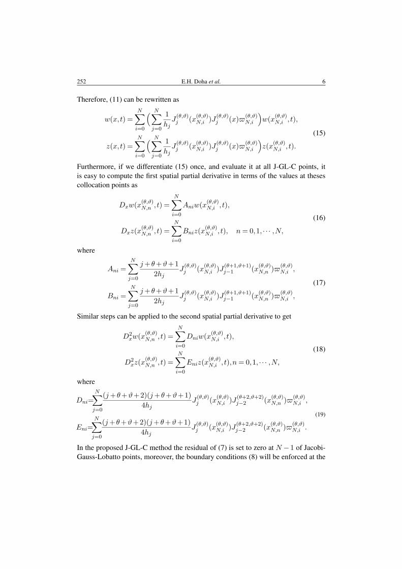
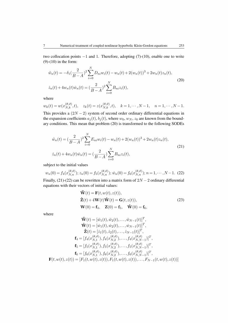
Fig. 1 – The approximate solution u(x,t) for problem (27) where θ= ϑ=0 and N =20 in the interval[−π,π].
-3 -2 -1 0 1 2 30.0
0.2
0.4
0.6
0.8
1.0
x
Exacte
and
approxim
ate
solu
tions
u�
Hx,0.9L
uHx,0.9L
u�
Hx,0.5L
uHx,0.5L
u�
Hx,0.1L
uHx,0.1L
0.70 0.75 0.80 0.85 0.900.80
0.82
0.84
0.86
0.88
x
Exacte
and
approxim
ate
solu
tions
u�
Hx,0.9L
uHx,0.9L
u�
Hx,0.5L
uHx,0.5L
u�
Hx,0.1L
uHx,0.1L
a b
Fig. 2 – The approximate solution u(x,t) and the exact solution u(x,t) for t = 0.1, 0.5, and 0.9 forproblem (27) where θ = ϑ= 0 and N = 24 in the interval [−π,π].
RJP 59(Nos. 3–4), 247–264 (2014) (c) 2014-2014
256 E.H. Doha et al. 10
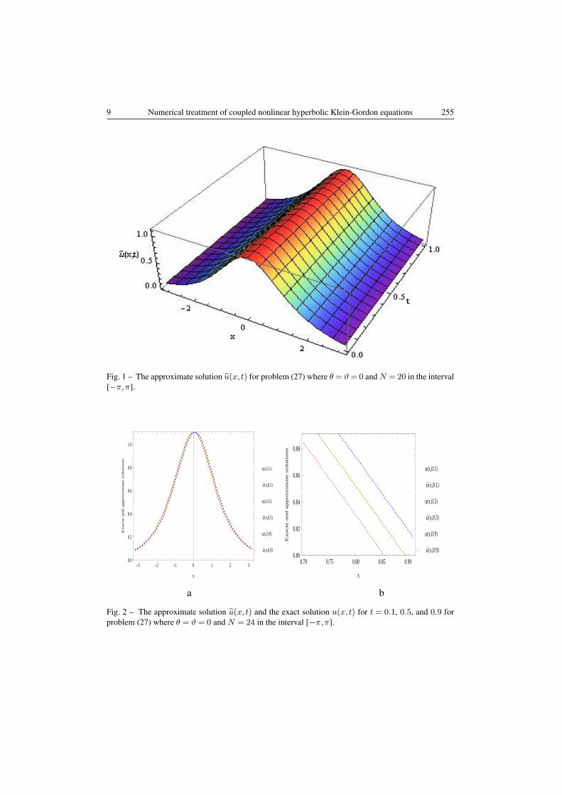
Fig. 3 – The approximate solution v(x,t) for problem (27) where θ= ϑ=0 and N = 20 in the interval[−π,π].
-3 -2 -1 0 1 2 3
-0.20
-0.15
-0.10
-0.05
0.00
x
Exacte
and
approxim
ate
solu
tions
v�
Hx,0.9L
vHx,0.9L
v�
Hx,0.5L
vHx,0.5L
v�
Hx,0.1L
vHx,0.1L
0.50 0.55 0.60 0.65 0.70
-0.19
-0.18
-0.17
-0.16
-0.15
x
Ex
acte
an
dap
pro
xim
ate
so
luti
on
s
v�
Hx,0.9L
vHx,0.9L
v�
Hx,0.5L
vHx,0.5L
v�
Hx,0.1L
vHx,0.1L
a b
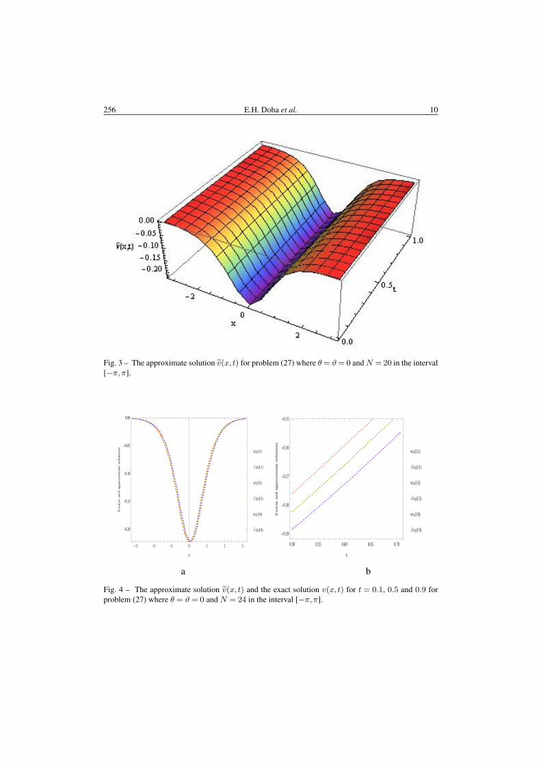
Fig. 4 – The approximate solution v(x,t) and the exact solution v(x,t) for t = 0.1, 0.5 and 0.9 forproblem (27) where θ = ϑ= 0 and N = 24 in the interval [−π,π].
RJP 59(Nos. 3–4), 247–264 (2014) (c) 2014-2014
11 Numerical treatment of coupled nonlinear hyperbolic Klein-Gordon equations 257
-3 -2 -1 0 1 2 30.0
0.2
0.4
0.6
0.8
1.0
x
Ex
acte
and
app
rox
imat
eso
luti
on
s
u�
Hx,0.9L
uHx,0.9L
u�
Hx,0.5L
uHx,0.5L
u�
Hx,0.1L
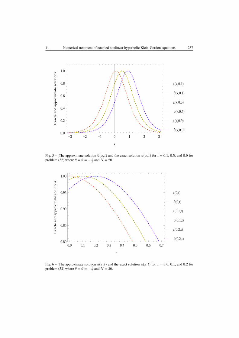
uHx,0.1L
Fig. 5 – The approximate solution u(x,t) and the exact solution u(x,t) for t = 0.1, 0.5, and 0.9 forproblem (32) where θ = ϑ=− 1
2 and N = 20.
0.0 0.1 0.2 0.3 0.4 0.5 0.6 0.70.80
0.85
0.90
0.95
1.00
t
Ex
acte
and
app
rox
imat
eso
luti
on
s
u�
H0.2,tL
uH0.2,tL
u�
H0.1,tL
uH0.1,tL
u�
H0,tL
uH0,tL
Fig. 6 – The approximate solution u(x,t) and the exact solution u(x,t) for x = 0.0, 0.1, and 0.2 forproblem (32) where θ = ϑ=− 1
2 and N = 20.
RJP 59(Nos. 3–4), 247–264 (2014) (c) 2014-2014
258 E.H. Doha et al. 12
-3 -2 -1 0 1 2 30.0
0.2
0.4
0.6
0.8
1.0
x
Ex
acte
and
app
rox
imat
eso
luti
on
s
v�
Hx,0.9L
vHx,0.9L
v�
Hx,0.5L
vHx,0.5L
v�
Hx,0.1L
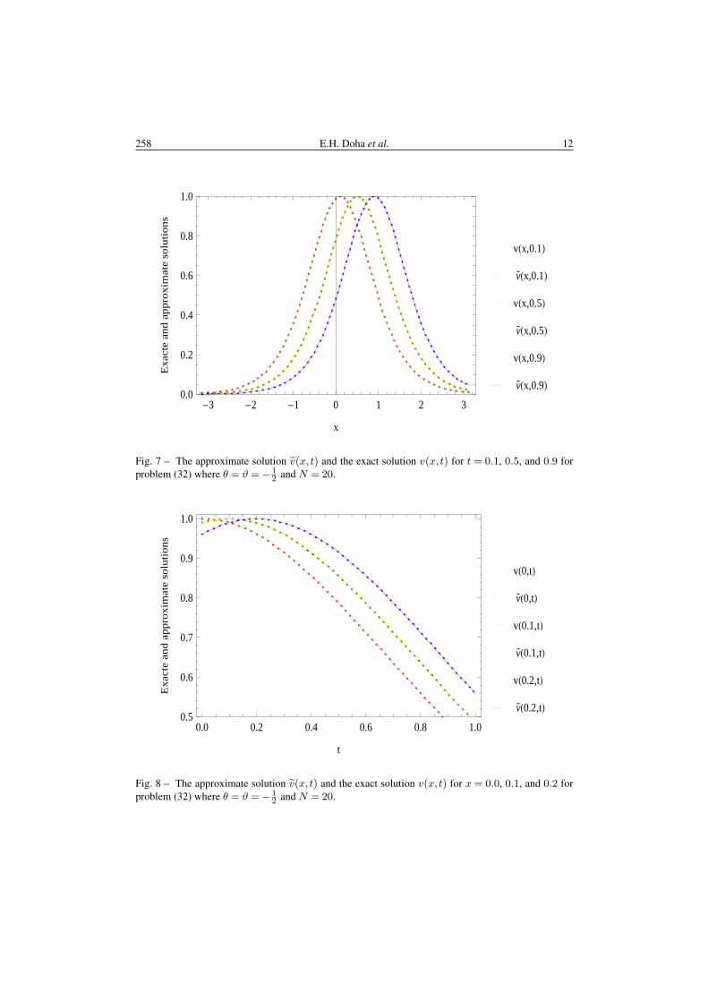
vHx,0.1L
Fig. 7 – The approximate solution v(x,t) and the exact solution v(x,t) for t = 0.1, 0.5, and 0.9 forproblem (32) where θ = ϑ=− 1
2 and N = 20.
0.0 0.2 0.4 0.6 0.8 1.00.5
0.6
0.7
0.8
0.9
1.0
t
Ex
acte
and
app
rox
imat
eso
luti
on
s
v�
H0.2,tL
vH0.2,tL
v�
H0.1,tL
vH0.1,tL
v�
H0,tL
vH0,tL
Fig. 8 – The approximate solution v(x,t) and the exact solution v(x,t) for x = 0.0, 0.1, and 0.2 forproblem (32) where θ = ϑ=− 1
2 and N = 20.
RJP 59(Nos. 3–4), 247–264 (2014) (c) 2014-2014
13 Numerical treatment of coupled nonlinear hyperbolic Klein-Gordon equations 259
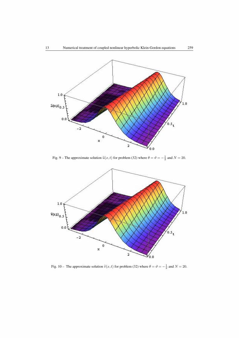
Fig. 9 – The approximate solution u(x,t) for problem (32) where θ = ϑ=− 12 and N = 20.
Fig. 10 – The approximate solution v(x,t) for problem (32) where θ = ϑ=− 12 and N = 20.
RJP 59(Nos. 3–4), 247–264 (2014) (c) 2014-2014
260 E.H. Doha et al. 14
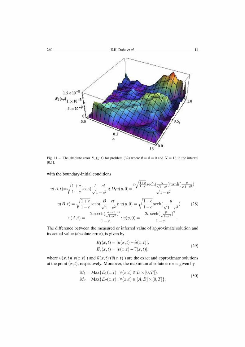
Fig. 11 – The absolute error E1(y,t) for problem (32) where θ = ϑ = 0 and N = 16 in the interval[0,1].
with the boundary-initial conditions
u(A,t)=
√1+ c
1− csech(
A− ct√1− c2
);Dtu(y,0)=c√
1+c1−c sech(
y√1−c2
)tanh( y√1−c2
)√1− c2
u(B,t) =
√1+ c
1− csech(
B− ct√1− c2
); u(y,0) =
√1+ c
1− csech(
y√1− c2
) (28)
v(A,t) =−2c sech( a−ct√
1−c2)2
1− c; v(y,0) =−
2c sech( y√1−c2
)2
1− c.
The difference between the measured or inferred value of approximate solution andits actual value (absolute error), is given by
E1(x,t) = |u(x,t)− u(x,t)|,E2(x,t) = |v(x,t)− v(x,t)|,
(29)
where u(x,t)( v(x,t) ) and u(x,t) (v(x,t) ) are the exact and approximate solutionsat the point (x,t), respectively. Moreover, the maximum absolute error is given by
M1 = Max{E1(x,t) : ∀(x,t) ∈D× [0,T ]},M2 = Max{E2(x,t) : ∀(x,t) ∈ [A,B]× [0,T ]}.
(30)
RJP 59(Nos. 3–4), 247–264 (2014) (c) 2014-2014
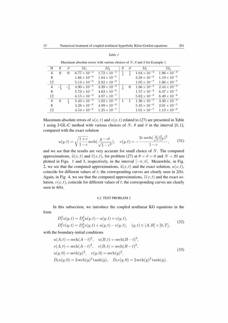
15 Numerical treatment of coupled nonlinear hyperbolic Klein-Gordon equations 261
Table 1
Maximum absolute errors with various choices of N , θ and ϑ for Example 1.
N θ ϑ M1 M2 θ ϑ M1 M2
4 0 0 6.77×10⁻⁴ 1.72×10⁻³ 12
12 1.04×10⁻³ 1.96×10⁻³
8 1.66×10⁻⁶ 1.04×10⁻⁵ 3.28×10⁻⁶ 1.19×10⁻⁵
12 5.14×10⁻⁹ 2.82×10⁻⁸ 1.05×10⁻⁷ 1.66×10⁻⁷
4 - 12 - 12 4.90×10⁻⁴ 3.39×10⁻³ 12 0 1.66×10⁻³ 2.44×10⁻³
8 5.73×10⁻⁷ 4.63×10⁻⁶ 1.57×10⁻⁶ 6.47×10⁻⁵
12 4.15×10⁻⁹ 4.87×10⁻⁷ 5.62×10⁻⁸ 6.49×10⁻⁸
4 0 12 5.43×10⁻⁴ 1.02×10⁻³ 1 1 1.36×10⁻³ 3.30×10⁻³
8 4.28×10⁻⁶ 4.89×10⁻⁶ 5.45×10⁻⁶ 2.01×10⁻⁵
12 4.54×10⁻⁸ 1.25×10⁻⁷ 1.01×10⁻⁷ 1.13×10⁻⁶
Maximum absolute errors of u(x,t) and v(x,t) related to (27) are presented in Table1 using J-GL-C method with various choices of N , θ and ϑ in the interval [0,1],compared with the exact solution
u(y,t) =
√1+ c
1− csech(
y− ct√1− c2
), v(y,t) =−2c sech( y−ct√
1−c2)2
1− c, (31)
and we see that the results are very accurate for small choice of N . The computedapproximations, u(x,t) and v(x,t), for problem (27) at θ = ϑ = 0 and N = 20 areplotted in Figs. 1 and 3, respectively, in the interval [−π,π]. Meanwhile, in Fig.2, we see that the computed approximations, u(x,t) and the exact solution, u(x,t),coincide for different values of t; the corresponding curves are clearly seen in 2(b).Again, in Fig. 4, we see that the computed approximations, v(x,t) and the exact so-lution, v(x,t), coincide for different values of t; the corresponding curves are clearlyseen in 4(b).
4.2. TEST PROBLEM 2
In this subsection, we introduce the coupled nonlinear KG equations in theform
D2t u(y,t) =D2
yu(y, t)−u(y,t)+v(y,t),
D2t v(y,t) =D2
yv(y,t)+u(y,t)−v(y,t), (y,t) ∈ [A,B]× [0,T ],(32)
with the boundary-initial conditions
u(A,t) = sech(A− t)2, u(B,t) = sech(B− t)2,
v(A,t) = sech(A− t)2, v(B,t) = sech(B− t)2,
u(y,0) = sech(y)2, v(y,0) = sech(y)2,
Dtu(y,0) = 2sech(y)2 tanh(y), Dtv(y,0) = 2sech(y)2 tanh(y).
(33)
RJP 59(Nos. 3–4), 247–264 (2014) (c) 2014-2014
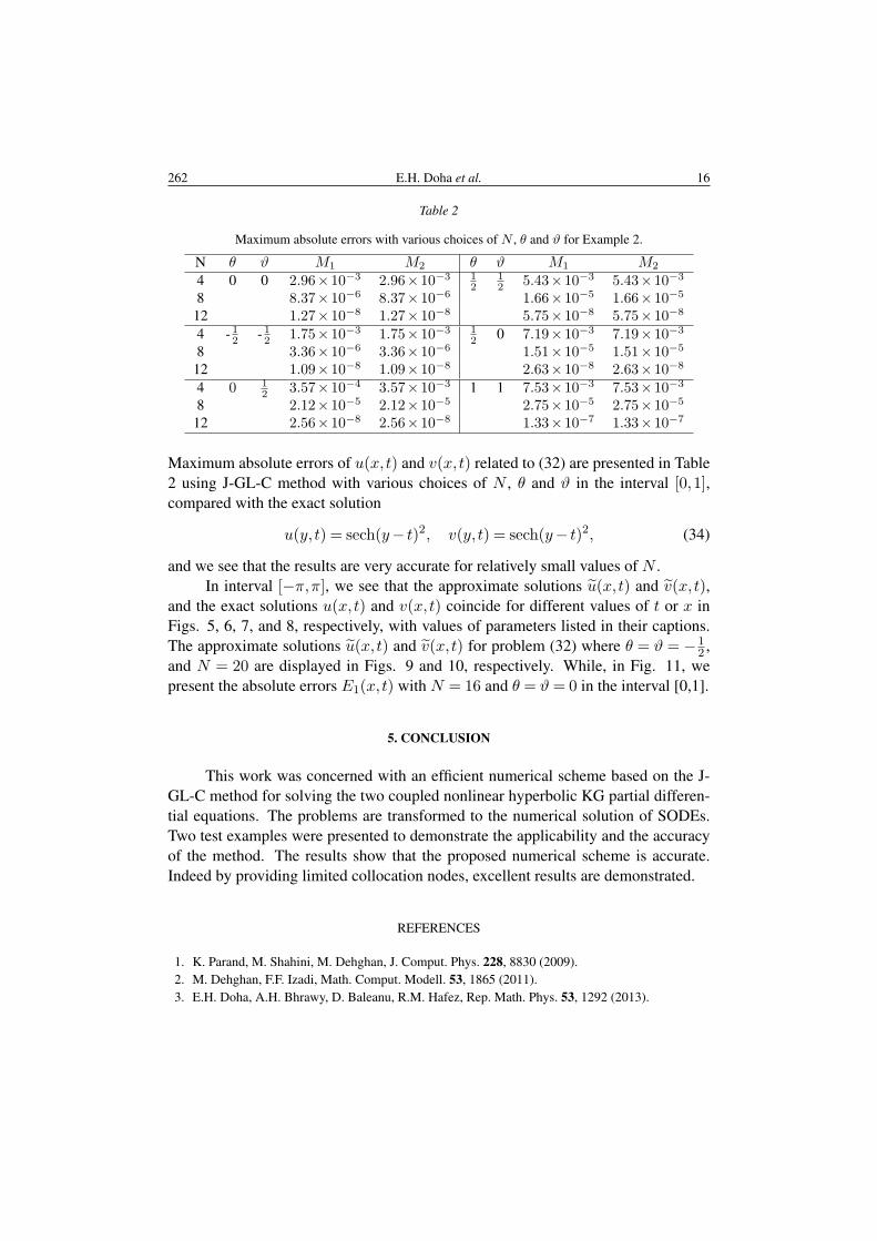
262 E.H. Doha et al. 16
Table 2
Maximum absolute errors with various choices of N , θ and ϑ for Example 2.
N θ ϑ M1 M2 θ ϑ M1 M2
4 0 0 2.96×10⁻³ 2.96×10⁻³ 12
12 5.43×10⁻³ 5.43×10⁻³
8 8.37×10⁻⁶ 8.37×10⁻⁶ 1.66×10⁻⁵ 1.66×10⁻⁵
12 1.27×10⁻⁸ 1.27×10⁻⁸ 5.75×10⁻⁸ 5.75×10⁻⁸
4 - 12 - 12 1.75×10⁻³ 1.75×10⁻³ 12 0 7.19×10⁻³ 7.19×10⁻³
8 3.36×10⁻⁶ 3.36×10⁻⁶ 1.51×10⁻⁵ 1.51×10⁻⁵
12 1.09×10⁻⁸ 1.09×10⁻⁸ 2.63×10⁻⁸ 2.63×10⁻⁸
4 0 12 3.57×10⁻⁴ 3.57×10⁻³ 1 1 7.53×10⁻³ 7.53×10⁻³
8 2.12×10⁻⁵ 2.12×10⁻⁵ 2.75×10⁻⁵ 2.75×10⁻⁵
12 2.56×10⁻⁸ 2.56×10⁻⁸ 1.33×10⁻⁷ 1.33×10⁻⁷
Maximum absolute errors of u(x,t) and v(x,t) related to (32) are presented in Table2 using J-GL-C method with various choices of N , θ and ϑ in the interval [0,1],compared with the exact solution
u(y,t) = sech(y− t)2, v(y,t) = sech(y− t)2, (34)
and we see that the results are very accurate for relatively small values of N .In interval [−π,π], we see that the approximate solutions u(x,t) and v(x,t),
and the exact solutions u(x,t) and v(x,t) coincide for different values of t or x inFigs. 5, 6, 7, and 8, respectively, with values of parameters listed in their captions.The approximate solutions u(x,t) and v(x,t) for problem (32) where θ = ϑ = −1
2 ,and N = 20 are displayed in Figs. 9 and 10, respectively. While, in Fig. 11, wepresent the absolute errors E1(x,t) with N = 16 and θ = ϑ= 0 in the interval [0,1].
5. CONCLUSION
This work was concerned with an efficient numerical scheme based on the J-GL-C method for solving the two coupled nonlinear hyperbolic KG partial differen-tial equations. The problems are transformed to the numerical solution of SODEs.Two test examples were presented to demonstrate the applicability and the accuracyof the method. The results show that the proposed numerical scheme is accurate.Indeed by providing limited collocation nodes, excellent results are demonstrated.
REFERENCES
1. K. Parand, M. Shahini, M. Dehghan, J. Comput. Phys. 228, 8830 (2009).2. M. Dehghan, F.F. Izadi, Math. Comput. Modell. 53, 1865 (2011).3. E.H. Doha, A.H. Bhrawy, D. Baleanu, R.M. Hafez, Rep. Math. Phys. 53, 1292 (2013).
RJP 59(Nos. 3–4), 247–264 (2014) (c) 2014-2014
17 Numerical treatment of coupled nonlinear hyperbolic Klein-Gordon equations 263
4. Y. Ordokhani, M. Razzaghi, Appl. Math. Lett. 21, 4 (2008).5. K. Zhang, J. Li, H. Song, Appl. Math. Comput. 218, 10848 (2012).6. Y. Jiang, J. Ma, J. Comput. Appl. Math. 244, 115 (2013).7. S. Yuzbasi, M. Sezer, B. Kemanci, Appl. Math. Mod. 37, 2086 (2013).8. A.H. Bhrawy, M.M. Tharwat, A. Yildirim, Appl. Math. Mod. 37, 4245 (2013).9. D. Baleanu, A.H. Bhrawy, T.M. Taha, Abstr. Appl. Anal., 2013, Article ID 546502 (2013)
10. C. Canuto, M.Y. Hussaini, A. Quarteroni, T.A. Zang, Spectral Methods: Fundamentals in SingleDomains (Springer-Verlag, New York, 2006).
11. J.K. Perring, T.H. Skyrme, Nuclear Phys. 31, 550 (1962).12. B.A. Malomed et al., J. Opt. B: Quantum Semiclassical Opt. 7, R53 (2005);
Y.V. Kartashov et al., Opt. Lett. 31, 2329 (2006);D. Mihalache et al., Opt. Commun. 137, 113 (1997);D. Mihalache, F. Lederer, D. Mazilu, L.-C. Crasovan, Opt. Eng. 35, 1616 (1996);Y.V. Kartashov, B.A. Malomed, L. Torner, Rev. Mod. Phys. 83, 247 (2011).
13. D. Mihalache, Rom. J. Phys. 57, 352 (2012);G. Ebadi et al., Proc. Romanian Acad. A 13, 215 (2012);A.G. Johnpillai, A. Yildirim, A. Biswas, Rom. J. Phys. 57, 545 (2012);A. Jafarian et al., Rom. Rep. Phys. 65, 76 (2013).
14. H. Leblond, D. Mihalache, Phys. Reports 523, 61 (2013);Y.J. He, D. Mihalache, Rom. Rep. Phys. 64, 1243 (2012);Guangye Yang et al., Rom. Rep. Phys. 65, 391 (2013);G. Ebadi et al., Rom. J. Phys. 58, 3 (2013).
15. Changming Huang, Chunyan Li, Haidong Liu, Liangwei Dong, Proc. Romanian Acad. A 13, 329(2012);Li Chen, Rujiang Li, Na Yang, Da Chen, Lu Li, Proc. Romanian Acad. A 13, 46 (2012);H. Triki et al., Proc. Romanian Acad. A 13, 103 (2012).
16. P.J. Caudrey, I.C. Eilbeck, J.D. Gibbon, Nuovo Cimento 25, 497 (1975).17. A.D. Polyanin, V.E. Zaitsev, Handbook of Nonlinear Partial Differential Equations (Chapman &
Hall/CRC, Boca Raton, 2004)18. K. Porsezian, T. Alagesan, Phys. Lett. A 198, 378 (1995).19. T. Alagesan, Y. Chung, K. Nakkeeran, Chaos, Solitons and Fractals 21, 879 (2004).20. E. Yusufoglu, A. Bekir, Math. Comput. Modell. 48, 1694 (2008).21. A.-M. Wazwaz, Chaos, Solitons and Fractals 28, 1005 (2006).22. A.-M. Wazwaz, Commun. Nonlinear Sci. 13, 889 (2008).23. Q. Shi, Q. Xiao, X. Liu, Appl. Math. Comput. 218, 9922 (2012).24. K. Khan, M.A. Akbar, J. Associat. Arab Univer. Basic Appl. Sci., in press (2013).25. M. Russo, R.A. Van Gorder, S. Roy Choudhury, Commun. Nonlinear Sci. 18, 1623 (2013).26. Z-Y. Zhang, J. Zhong, S.S. Dou, J. Liu, D. Peng, T. Gao, Rom. J. Phys. 58, 749 (2013).27. Z-Y. Zhang, J. Zhong, S.S. Dou, J. Liu, D. Peng, T. Gao, Rom. J. Phys. 58, 766 (2013).28. G. Murariu, A. Ene, Rom. J. Phys. 53, 651 (2008).29. E.H. Doha, A.H. Bhrawy, Comput. Math. Appl. 64, 558 (2012).30. E.H. Doha, A.H. Bhrawy, R.M. Hafez, M.A. Abdelkawy, Appl. Math. Inf. Sci. 8, 1 (2014).31. A.H. Bhrawy, L.M. Assas, M.A. Alghamdi, Bound. Value Probl. 2013, 87 (2013)32. A.H. Bhrawy, L.M. Assas, M.A. Alghamdi, Abstr. Appl. Anal., 2013, Article ID 741278 (2013).33. X.J. Yang, D. Baleanu, W.P. Zhong, Proc. Romanian. Acad. A 14, 127 (2013);
A.K. Golmankhaneh, N.A. Porghoveh, D. Baleanu, Rom. Rep. Phys. 65, 350 (2013);
RJP 59(Nos. 3–4), 247–264 (2014) (c) 2014-2014
264 E.H. Doha et al. 18
D. Rostamy, M. Alipour, H. Jafari, D. Baleanu, Rom. Rep. Phys. 65, 334 (2013).34. E.Y. Deeba, S.A. Khuri, J. Comp. Phys. 124, 442 (1996).35. E. Yusufoglu, Appl. Math. Lett. 21, 669 (2008).36. A.S.V. Ravi Kanth, K. Aruna, Comput. Phys. Commun. 180, 708 (2009).37. S. Iqbal, M. Idrees, A.M. Siddiqui, A.R. Ansari, Appl. Math. Comput. 216, 2898 (2010).38. S.A. Khuri, A. Sayfy, Appl. Math. Comput. 216, 1047 (2010).39. M.A.M. Lynch, Appl. Numer. Math. 31, 173 (1999).40. X. Li, B. Y. Guo, L. Vazquez, Math. Appl. Comput. 15, 19 (1996).41. X. Li, B.Y. Guo, J. Comp. Math. 15, 105 (1997).42. M. Dehghan, A. Shokri, J. Comput. Appl. Math. 230, 400 (2009).43. J. Rashidinia, M. Ghasemi, R. Jalilian, J. Comput. Appl. Math. 233, 1866 (2010).44. A.H. Bhrawy, Appl. Math. Comput. 222, 255 (2013)45. E.H. Doha, A.H. Bhrawy, R.M. Hafez, Math. Comput. Modell. 53, 1820 (2011).46. E.H. Doha, A.H. Bhrawy, R.M. Hafez, Abstr. Appl. Anal., 2011, Article ID 947230 (2011).47. G. Szego, Orthogonal Polynomials (Colloquium Publications XXIII, American Mathematical So-
ciety, ISBN 978-0-8218-1023-1, MR 0372517, 1939).
RJP 59(Nos. 3–4), 247–264 (2014) (c) 2014-2014