observational and numerical modeling methods for...

Available online at www.sciencedirect.com

Progress in Oceanography 76 (2008) 399–442

Progress inOceanography

www.elsevier.com/locate/pocean

Review

Observational and numerical modeling methods forquantifying coastal ocean turbulence and mixing

Hans Burchard a,*, Peter D. Craig b, Johannes R. Gemmrich c, Hans van Haren d,Pierre-Philippe Mathieu e, H.E. Markus Meier f, W. Alex M. Nimmo Smith g,

Hartmut Prandke h, Tom P. Rippeth i, Eric D. Skyllingstad j, William D. Smyth j,David J.S. Welsh k,1, Hemantha W. Wijesekera j

a Department for Physical Oceanography and Instrumentation, Leibniz Institute for Baltic Sea Research Warnemunde, Seestraße 15,

D-18119 Rostock-Warnemunde, Germanyb CSIRO Marine and Atmospheric Research, G.P.O. Box 1538, Hobart, Tas. 7001, Australia

c University of Victoria, Physics and Astronomy, P.O. Box 3055, Victoria, BC, Canada V8W 3P6d Royal Netherlands Institute for Sea Research, P.O. Box 59, NL-1790 AB Den Burg, Texel, The Netherlands

e European Space Agency, ESA/ESRIN, Via Galileo Galilei, I-00044 Frascati, Italyf Swedish Meteorological and Hydrological Institute, SE-601 76 Norrkoping, Sweden

g University of Plymouth, School of Earth, Ocean and Environmental Sciences, Drake Circus, Plymouth PL4 8AA, United Kingdomh ISW Wassermesstechnik, Gartenweg 1, D-17213 Funfseen, Germany

i School of Ocean Sciences, Menai Bridge, College of Natural Sciences, Bangor University, Anglesey LL59 5AB, United Kingdomj Oregon State University, College of Ocean and Atmospheric Sciences, 104 COAS Administration Building, Corvallis, OR 97331-5503, USA

k Ohio State University, Department of Civil and Environmental Engineering and Geodetic Science, 470 Hitchcock Hall,

2070 Neil Avenue, Columbus, OH 43210, USA

Received 7 February 2007; accepted 28 September 2007Available online 26 January 2008

Abstract

In this review paper, state-of-the-art observational and numerical modeling methods for small scale turbulence and mix-ing with applications to coastal oceans are presented in one context. Unresolved dynamics and remaining problems of fieldobservations and numerical simulations are reviewed on the basis of the approach that modern process-oriented studiesshould be based on both observations and models. First of all, the basic dynamics of surface and bottom boundary layersas well as intermediate stratified regimes including the interaction of turbulence and internal waves are briefly discussed.Then, an overview is given on just established or recently emerging mechanical, acoustic and optical observational tech-niques. Microstructure shear probes although developed already in the 1970s have only recently become reliable commer-cial products. Specifically under surface waves turbulence measurements are difficult due to the necessary decomposition ofwaves and turbulence. The methods to apply Acoustic Doppler Current Profilers (ADCPs) for estimations of Reynoldsstresses, turbulence kinetic energy and dissipation rates are under further development. Finally, applications of well-estab-lished turbulence resolving particle image velocimetry (PIV) to the dynamics of the bottom boundary layer are presented.As counterpart to the field methods the state-of-the-art in numerical modeling in coastal seas is presented. This includes the

0079-6611/$ - see front matter � 2008 Elsevier Ltd. All rights reserved.

doi:10.1016/j.pocean.2007.09.005

* Corresponding author. Tel.: +49 381 5197 140; fax: +49 381 5197 114.E-mail address: [email protected] (H. Burchard).

1 Present address: Innovative Management and Technology Services, 2900 Presidential Drive, Suite 170, Fairborn, OH 45324, USA.

mailto:[email protected]

400 H. Burchard et al. / Progress in Oceanography 76 (2008) 399–442

application of the Large Eddy Simulation (LES) method to shallow water Langmuir Circulation (LC) and to stratified flowover a topographic obstacle. Furthermore, statistical turbulence closure methods as well as empirical turbulence parame-terizations and their applicability to coastal ocean turbulence and mixing are discussed. Specific problems related to thecombined wave–current bottom boundary layer are discussed. Finally, two coastal modeling sensitivity studies are pre-sented as applications, a two-dimensional study of upwelling and downwelling and a three-dimensional study for a mar-ginal sea scenario (Baltic Sea). It is concluded that the discussed methods need further refinements specifically to accountfor the complex dynamics associated with the presence of surface and internal waves.� 2008 Elsevier Ltd. All rights reserved.

Keywords: Coastal oceanography; Turbulent fluxes; Micro-structure measurements; Acoustic turbulence measurements; Turbulencemodeling; Shelf sea modeling

Contents

1. Introduction . . . . . . . . . . . . . . . . . . . . . . . . . . . . . . . . . . . . . . . . . . . . . . . . . . . . . . . . . . . . . . . . . . . . 4012. Turbulent regimes . . . . . . . . . . . . . . . . . . . . . . . . . . . . . . . . . . . . . . . . . . . . . . . . . . . . . . . . . . . . . . . . 401

2.1. Surface boundary layer . . . . . . . . . . . . . . . . . . . . . . . . . . . . . . . . . . . . . . . . . . . . . . . . . . . . . . . 4012.2. Bottom boundary layer . . . . . . . . . . . . . . . . . . . . . . . . . . . . . . . . . . . . . . . . . . . . . . . . . . . . . . . 403

2.2.1. Steady and tidal flow . . . . . . . . . . . . . . . . . . . . . . . . . . . . . . . . . . . . . . . . . . . . . . . . . . . 4032.2.2. Wave–current bottom boundary layer . . . . . . . . . . . . . . . . . . . . . . . . . . . . . . . . . . . . . . . 4042.2.3. Effects of sediment . . . . . . . . . . . . . . . . . . . . . . . . . . . . . . . . . . . . . . . . . . . . . . . . . . . . . 404

2.3. Internal waves and turbulence . . . . . . . . . . . . . . . . . . . . . . . . . . . . . . . . . . . . . . . . . . . . . . . . . . 405
3. Observation and data interpretation . . . . . . . . . . . . . . . . . . . . . . . . . . . . . . . . . . . . . . . . . . . . . . . . . . . 407
3.1. Micro-structure shear-probe observations. . . . . . . . . . . . . . . . . . . . . . . . . . . . . . . . . . . . . . . . . . . 408
3.1.1. Problems, limitations and measurement strategy . . . . . . . . . . . . . . . . . . . . . . . . . . . . . . . . 4083.1.2. Example of measurements . . . . . . . . . . . . . . . . . . . . . . . . . . . . . . . . . . . . . . . . . . . . . . . . 409
3.2. Observing turbulence beneath breaking waves . . . . . . . . . . . . . . . . . . . . . . . . . . . . . . . . . . . . . . . 4093.3. Near-bed high-resolution ADCP data . . . . . . . . . . . . . . . . . . . . . . . . . . . . . . . . . . . . . . . . . . . . . 411

3.3.1. The variance method . . . . . . . . . . . . . . . . . . . . . . . . . . . . . . . . . . . . . . . . . . . . . . . . . . . 412
3.4. Particle image velocimetry in the BBL . . . . . . . . . . . . . . . . . . . . . . . . . . . . . . . . . . . . . . . . . . . . . 415
3.4.1. Instrumentation . . . . . . . . . . . . . . . . . . . . . . . . . . . . . . . . . . . . . . . . . . . . . . . . . . . . . . 4153.4.2. Example data . . . . . . . . . . . . . . . . . . . . . . . . . . . . . . . . . . . . . . . . . . . . . . . . . . . . . . . . 4163.4.3. Estimating the Reynolds stress . . . . . . . . . . . . . . . . . . . . . . . . . . . . . . . . . . . . . . . . . . . . 416

4. Modeling . . . . . . . . . . . . . . . . . . . . . . . . . . . . . . . . . . . . . . . . . . . . . . . . . . . . . . . . . . . . . . . . . . . . . 417
4.1. Large eddy simulation . . . . . . . . . . . . . . . . . . . . . . . . . . . . . . . . . . . . . . . . . . . . . . . . . . . . . . . . 419
4.1.1. Coastal applications . . . . . . . . . . . . . . . . . . . . . . . . . . . . . . . . . . . . . . . . . . . . . . . . . . . . 420
4.2. Statistical turbulence closure models . . . . . . . . . . . . . . . . . . . . . . . . . . . . . . . . . . . . . . . . . . . . . . 422
4.2.1. Basic principles. . . . . . . . . . . . . . . . . . . . . . . . . . . . . . . . . . . . . . . . . . . . . . . . . . . . . . . . 4224.2.2. One- and two-equation models . . . . . . . . . . . . . . . . . . . . . . . . . . . . . . . . . . . . . . . . . . . . 4234.2.3. Unresolved processes . . . . . . . . . . . . . . . . . . . . . . . . . . . . . . . . . . . . . . . . . . . . . . . . . . . 4244.2.4. Example application . . . . . . . . . . . . . . . . . . . . . . . . . . . . . . . . . . . . . . . . . . . . . . . . . . . . 425

4.3. Empirical turbulence models. . . . . . . . . . . . . . . . . . . . . . . . . . . . . . . . . . . . . . . . . . . . . . . . . . . . 427
4.3.1. The K-profile parameterization . . . . . . . . . . . . . . . . . . . . . . . . . . . . . . . . . . . . . . . . . . . . 428
4.4. Modeling the wave–current bottom boundary layer . . . . . . . . . . . . . . . . . . . . . . . . . . . . . . . . . . . 429
4.4.1. The Grant and Madsen approach . . . . . . . . . . . . . . . . . . . . . . . . . . . . . . . . . . . . . . . . . . 4294.4.2. High-resolution modeling . . . . . . . . . . . . . . . . . . . . . . . . . . . . . . . . . . . . . . . . . . . . . . . . 430
4.5. Sensitivity of 2D and 3D model results to turbulence parameterizations . . . . . . . . . . . . . . . . . . . . . 430
4.5.1. A case study for the Baltic Sea . . . . . . . . . . . . . . . . . . . . . . . . . . . . . . . . . . . . . . . . . . . . 4304.5.2. Coastal upwelling and downwelling . . . . . . . . . . . . . . . . . . . . . . . . . . . . . . . . . . . . . . . . . 4334.5.3. Case study overview . . . . . . . . . . . . . . . . . . . . . . . . . . . . . . . . . . . . . . . . . . . . . . . . . . . . 435
5. Conclusions. . . . . . . . . . . . . . . . . . . . . . . . . . . . . . . . . . . . . . . . . . . . . . . . . . . . . . . . . . . . . . . . . . . . . 435Acknowledgements . . . . . . . . . . . . . . . . . . . . . . . . . . . . . . . . . . . . . . . . . . . . . . . . . . . . . . . . . . . . . . . 436References . . . . . . . . . . . . . . . . . . . . . . . . . . . . . . . . . . . . . . . . . . . . . . . . . . . . . . . . . . . . . . . . . . . . . . 436

H. Burchard et al. / Progress in Oceanography 76 (2008) 399–442 401

1. Introduction

Turbulence is an important mechanism for transporting heat, salt, momentum and suspended and dissolvedmatter in the coastal zone. The so-called turbulent fluxes of material occur as a result of correlated, small-scalefluctuations in current velocity and the transported quantity itself. Increasing turbulence usually leads toincreased turbulent fluxes as measured, for example, by the variance of the current velocity (a measure forthe turbulent kinetic energy (TKE)) and the variance of the transported quantity. The horizontal and verticalturbulent fluxes are typically of the same order of magnitude. Due to the small aspect ratio (the ratio of ver-tical to horizontal length scales) in natural waters, horizontal advective fluxes caused by the mean flow dom-inate horizontal turbulent fluxes. Horizontal dispersion that has the characteristics of horizontal mixing resultsfrom shear dispersion, the joint effect of vertical mixing and differential horizontal advection due to currentshear.

Turbulence is produced either by mean shear (loss of mean-flow kinetic energy) or by unstable stratifica-tion (loss of potential energy). An external source of turbulence is breaking surface waves which inject tur-bulence into the water column. In the coastal zone, mean shear is typically generated by winds or tides, butalso by surface waves (Stokes drift) and baroclinic flows, including nonlinear internal waves. Unstable strat-ification results from surface processes such as surface cooling, evaporation or freezing and also as a result ofdifferential advection. In the latter, vertically well-mixed waters become unstably stratified through currentshear in situations such as upwelling zones, tidal estuaries and coastal areas during flood. Destruction ofturbulence occurs by transformation into potential energy (during stable stratification) or viscous dissipationinto heat.

Because of their statistical character, turbulent fluxes are difficult to observe, and must usually be quantifiedby indirect strategies. Often, observers measure turbulent statistics such as the vorticity variance (proportionalto the dissipation rate of TKE), the Reynolds stress or the temperature variance. With the aid of simplifyingassumptions (for example, the concept of eddy viscosity), measured quantities become estimators for the ver-tical turbulent fluxes. Numerical models incorporate parameterizations for quantifying turbulent fluxes. Thequality of these parameterizations is tested by their ability to reproduce certain observable turbulent behavior.

It is the intention of this paper to give an overview of relevant processes, observational techniques andmodeling strategies. The first two sections generally introduce the dynamics of the surface mixed layer (Section2.1) and the bottom boundary layer (Section 2.2). The complex interaction between turbulence and internalwaves is then discussed in Section 2.3. The following sections cover observational techniques and their meth-ods of statistical data interpretation, in particular, micro-structure shear-probe profilers (Section 3.1), mea-surement under breaking surface waves (Section 3.2), near-bed Acoustic Doppler Current Profilers(ADCPs) (Section 3.3) and particle image velocimetry (PIV) (Section 3.4). In the modeling part, the methodof Large Eddy Simulation (LES) is introduced in Section 4.1, followed by statistical models (Section 4.2) andempirical models (Section 4.3). Specific attention is given to the modeling of the wave–current bottom bound-ary layer, which is of high relevance in the coastal ocean, and combines both statistical and empiricalapproaches (Section 4.4). The paper concludes with a comparative study of two- and three-dimensional modelresults obtained from several empirical and statistical turbulence models (Section 4.5).

The dynamics of the coastal ocean is determined by a number of non-dimensional parameters and scalinglaws, some of which are explicitly discussed here. A far more comprehensive overview is given in the textbookof Kantha and Clayson (2000) in the Appendix C.

For the notation of velocity vector components, we define (u, v, w) = (u1, u2, u3) which mostly denote theeastward, the northward and the upward components, respectively.

2. Turbulent regimes

2.1. Surface boundary layer

The ocean surface boundary layer is the part of the ocean that is directly exposed to the atmosphere,through which atmospheric properties are transmitted into the ocean interior. It is the layer of the ocean inwhich there are high light levels, and therefore the potential for high biological productivity. Near-surface


turbulence creates a mixed layer immediately below the surface, in which quantities such as temperature anddissolved and particulate material are relatively uniform in the vertical.

Because of surface waves, there are significant differences between the ocean’s surface mixed layer and theatmospheric boundary layer (ABL). The surface mixed layer is usually more complex than the ABL with tur-bulence often not clearly separable from other coherent structures.

On both sides of the air–sea interface, there are thin skin layers of a few millimeter thickness that are notturbulent, but controlled by molecular viscosity and diffusivity. Although the skin layer thickness on the waterside is commonly only of the order of 1 mm it provides a significant bottle neck for many air–sea exchangeprocesses. The skin sea surface temperature (SSST), which is typically about 0.3 K lower than the bulkSST, determines heat losses to the cooler atmosphere (by processes of latent and sensible heat flux andlong-wave radiation, e.g. Taylor, 2000). The isolating skin layer is disrupted by breaking surface waves. Atlow to moderate wind speeds this occurs mainly in form of micro-breaking, that is, the breaking of very shortwind waves without air entrainment, which plays an important role in air–sea gas exchange (Zappa et al.,2001). Larger breaking waves cause whitecapping, that injects air bubbles into the water (and water dropsand spray into the air), so that the air–sea gas exchange increases tremendously at the location of breakers(e.g. Thorpe et al., 2003a).

At moderate to high wind speed, momentum is transferred from wind to ocean currents via wave breaking.The dissipation of wave energy occurs mainly in breaking waves. Thus, wave breaking is a source of enhancedTKE levels in the near-surface layer and plays an important role in upper ocean processes. Vertical transportof heat, gases and particles in the near-surface zone depends on turbulent transport. Generally, increased tur-bulence levels relate to enhanced air–sea exchange processes. Comprehensive overviews of the role of wave-induced turbulence in upper-ocean dynamics and air–sea exchange processes are given in a number of reviewarticles (Thorpe, 1995; Melville, 1996; Duncan, 2001).

It is now accepted that energy dissipation rates (denoted by e) in the near-surface layer of a wind-drivenocean depart significantly from the classic wall-layer form, in terms of magnitude as well as depth dependence.There is general agreement that in a wind-driven sea the surface layer may be divided into three regimes. Wavebreaking directly injects TKE into the top layer down to a depth zb. In this injection layer, dissipation rates arehighest and most probably independent of depth. Below zb, the wave-induced turbulence diffuses downwardsand dissipates. In this region, the turbulence decay rate is faster than the traditional wall-layer dependencee / z�1, which results from the assumption of a constant stress and zero surface flux of TKE, see also Eq.(10). At a depth zt, sufficiently far from the air–sea interface, the contribution of waves becomes small com-pared with local shear production, and turbulence properties are well described by the wall-layer scaling.There is, as yet, no conclusive observational evidence for the vertical extension of the different regimes (zb, zt),nor the exact depth-dependence of the wave-induced turbulence. Suggestions for the latter include e / zn, withn in the range �4 to �2 (Terray et al., 1996; Drennan et al., 1996), and e / e�z (Anis and Moum, 1995). In theopen ocean, under strong wind forcing in the presence of swell, Greenan et al. (2001) found enhanced dissi-pation rates but depth-dependence consistent with wall-layer scaling. The depth zb of direct TKE injectiondetermines the total dissipation rate, which in fully developed sea has to match the energy input from the wind(Gemmrich et al., 1994). Furthermore, zb determines the surface mixing length z0, a crucial parameter in tur-bulence closure models. The problem of properly observing zb is related to the spatial reference frame for themeasurements (see Section 3.2).

Other effects of surface waves are increased near-surface Reynolds stresses and related increases in horizon-tal transport due to Stokes drift. When the Stokes drift interacts with the wind-driven currents and the surfacemixed layer is not too deep, Langmuir circulation (LC) is triggered, see Thorpe et al. (2003a) and Rascle et al.(2006). LC is visible as characteristic surface windrows that are caused by bubble clouds in horizontal, coun-ter-rotating cells aligned in the wind direction. Since Langmuir cells are similar in size to large eddies, a stronginteraction between turbulence and Langmuir cells may be observed by means of LES, leading to a phenom-enon described as Langmuir turbulence (McWilliams et al., 1997 and also Section 4.1).

The major scaling parameter for turbulence in a wind-driven surface mixed layer is the surface frictionvelocity us

* = (ss/q)1/2, with the surface stress ss and the density q. When positive buoyancy fluxes due to cool-ing and evaporation come into play, another parameter is of great importance, the so-called Deardorff velocityscale w* = (B0D)1/3, where B0 is the surface buoyancy flux and D is the mixed layer depth. When the ratio


P� ¼ us�=w� falls below values of 0.65, the structure of the surface mixed layer becomes convectively domi-nated, with the typical counter-gradient fluxes of buoyancy (see the LES results by Moeng and Sullivan(1994) and Heitmann and Backhaus (2005)). The relevant non-dimensional quantity that determines theimportance of buoyancy fluxes in establishing LC is the Hoenikker number H O ¼ B0=ðk � u2

s� � V SOÞ, with thewave number k and the Stokes velocity VSO, see Li and Garrett (1995), Skyllingstad and Denbo (1995) andLi et al. (2005) for details.

The lower boundary of the surface mixed layer is either the seabed (in case the water is sufficiently shallow)or a pycnocline established by vertical gradients of temperature and/or salinity. In case of a pycnocline, inter-nal waves may be generated by various processes such as shear instability, large turbulent eddies, surfacewaves, spatial and temporal atmospheric forcing inhomogeneities, currents interacting with bottom topogra-phy. These internal waves will interact with turbulence (see Section 2.3).

In the case that the seabed is the lower boundary of the surface layer, the water column is completely mixed.This happens typically in tidally dominated coastal areas when the pycnocline is eroded from below. Simpsonand Hunter (1974) suggest a non-dimensional parameter of the form ð�HB0=�u3

�Þ (with depth H, surface buoy-ancy flux B0 and r.m.s. bed friction velocity �u�) as an estimator for whether the water column is mixed or strat-ified (see Simpson et al., 1977). As a rough and easily measurable indication for tidal front locations, Simpsonand Hunter (1974) use the dimensional ratio H=�u3

s , where �us denotes the surface velocity amplitude. WhenH=�us3 is in the order of a critical value of about 50–100 s3/m2, depending on the surface momentum and buoy-ancy fluxes, a frontal zone is expected nearby. Tidally induced frontal zones are known for complex mecha-nisms of cross-frontal circulation (see Dong et al., 2004) and high biological productivity (see Richardsonet al., 1998).

In shallow coastal water, the influence of surface waves may penetrate right to the bed and create a wavebottom boundary layer that can interact with the mean tidal (pressure-gradient-driven) or stress-driven flow(see Section 4.4 and observational evidence in Section 3.4). In contrast to a stress-driven flow, in a pressure-gradient-driven flow, the Reynolds stress might have a maximum value at the bottom boundary (see observa-tions of such well-mixed flows in Section 3.3).

2.2. Bottom boundary layer

In coastal regions, turbulent mixing near the marine bed is influenced by the interaction of current andwind-wave boundary layers and related sediment transport. A bottom boundary layer spans the vertical dis-tance between the no-slip bottom boundary condition and outer, free-stream motion. The height of theboundary layer is related to the magnitude of the free-stream velocity, bottom roughness and the time avail-able for boundary layer development. A wave boundary layer is typically much thinner, but far more turbu-lent, than a current boundary layer. When the two boundary layers co-exist, they interact in a transient,nonlinear manner, though the effect of currents on the wave boundary layer is generally much less than theeffect of waves on the current boundary layer.

2.2.1. Steady and tidal flow

Classic near-bed flow follows the law of the wall, leading to a logarithmic velocity profile which is deter-mined by the bed shear stress and a roughness length. (The roughness length is formally defined as the distanceabove the bed of the position at which the extrapolation of the logarithmic profile has zero velocity.) Such atypical wall layer will occur in stationary, unstratified and irrotational flows over plain, solid beds.

Natural bottom boundaries usually deviate significantly from the idealized picture of a wall layer. Beds arenot plain, but have ripples and dunes of various length scales, which contribute to an additional so-called formdrag. Seen from the body of the flow, ripples and dunes act as roughness elements in such a way that multiplelogarithmic layers may be observed (Soulsby, 1983). In shallow coastal waters, the oscillatory effect of surfacewaves on the bottom boundary layer may also significantly increase the effective bed roughness as felt from thebulk of the flow (see Section 2.2.2). Moreover, the bed does usually not consist of a hard substrate but par-ticulate sediments which may be suspended into the water column when bed stress is present. Thus, bed formsmay be influenced by the flow, density stratification caused by the sediment itself may damp near-bed turbu-lence, and down-slope density currents may be generated (Section 2.2.3).


Slowly varying flow such as tidal flow exhibits some peculiarities. When the water column is acceleratedfrom a situation in which the near-bed velocity is zero (as after slack tide), shear stress propagates upwardsfrom the bed. Other turbulent properties such as shear production, TKE and dissipation rate also propagateupwards, all with a height dependent time lag behind the phase of the bed stress. This has been clearly dem-onstrated by means of analytical models (e.g. Prandle, 1982), while observational evidence of the phase lag ofdissipation has been provided, for example, by Simpson et al. (2000). Recent independent observations of tur-bulence production and dissipation rate by Rippeth et al. (2003) in a narrow strait allow the study of the pro-duction-dissipation phase lag, which is often ignored in modeling exercises for boundary layer flow. Theturbulent structure of tidal bottom boundary layers may also be strongly influenced by horizontal density gra-dients. Due to tidal straining, turbulence is enhanced when the flow is towards water of lower density, and viceversa, as in the observations of Rippeth et al. (2001) and the simulations of Simpson et al. (2002). A modelsimulation of this effect is presented in Section 4.2.4.

2.2.2. Wave–current bottom boundary layer

In shallow coastal waters, the orbital motion due to surface waves may create horizontal oscillatory cur-rents in the near-bed region. Linear wave theory predicts significant near-bed orbital motions for water depthsless than 0:16gT 2

w, with Tw denoting the wave period, and g denoting the gravitational acceleration (see Souza,2005). Due to the rapid oscillatory nature of wave-induced motion, a wave boundary layer is typically muchsmaller in height (a few centimeters) than a current boundary layer (meters to tens of meters). This leads tosteeper velocity gradients and more intense turbulence in the wave boundary layer. When wave and currentboundary layers co-exist, the overlying currents appear to perceive the wave boundary layer as an additionalbed roughness contribution, leading to increased bottom friction and modified mean current profiles (Kempand Simons, 1982, 1983). As a result, the mean bottom stress in a combined flow is greater than the sum ofbottom stresses found in independent wave and current boundary layers.

Fig. 9 (Section 3.4) provides an example of the effect of waves on the mean current profile. For strong tidalcurrents dominating the motion near the bed, a classic logarithmic profile would be expected, with a straight-line portion that extends close to the bed. In contrast to that Fig. 9 shows how the effect of relatively weaktidal motion has led to a typical wave–current boundary layer profile, consistent with the form postulatedby Grant and Madsen (1986). The straight-line portions end well above the bed and one can estimate theapparent bottom roughness by extending these lines to intercept the velocity axis.

In recent decades, various model approaches towards simulating the wave–current bottom boundary layershave been suggested. Among these, the empirical theory of Grant and Madsen (1986) and its extensions havereceived the greatest attention in the scientific community. An alternative statistical approach consistent withstatistical turbulence closure models (Section 4.2) has recently been suggested by Mellor (2002). For a discus-sion of these models, see Section 4.4.

2.2.3. Effects of sediment

Sediment has three main effects on the structure of the bottom boundary layer: (i) variable bed forms, (ii)turbulence damping and (iii) generation of down-slope turbidity currents (for an overview see Friedrichs,2005).

The bed forms (ripples and dunes) are generated by means of a complex interaction between near-bed cur-rents and the seabed. For short-term investigations the impact of currents on bed forms may be neglected, buton longer time scales, this interaction may cause morphological modifications of coastal areas.

When the bottom shear stress of the current exceeds a certain critical value (which depends on a number offactors, including the bed shape, and sediment composition and compaction), sediment is eroded and resus-pended into the water column. At high sediment concentrations, the density of the sediment-laden water maybe such that significant stratification is generated, damping vertical turbulent mixing. For fine sediments withsmall settling velocities, a well-mixed sediment-laden layer may be generated, with a sharp vertical density gra-dient (a so-called lutocline, see Noh and Fernando, 1991) separating it from the non-turbid waters. If the sed-iment concentrations are high enough, the velocity profiles may deviate significantly from the law of the wall(see Friedrichs et al., 2000). The presence of a wave boundary layer will also enhance sediment entrainment(Glenn and Grant, 1987). Modeling of these effects is an area of current research (e.g. Winterwerp, 2001).


Downslope turbidity currents are generated when sediment is resuspended in a sloping bottom layer. Forsufficiently steep slopes, these currents may be self-accelerating, increasing the resuspension rate with increas-ing speed which, in turn, increases the speed with increasing density and sediment layer height. For a recentoverview over sediment gravity currents, see Parsons et al. (2007).

2.3. Internal waves and turbulence

In sufficiently deep shelf seas, well-mixed surface and bottom boundary layers may be separated by stablevertical density stratification. This stratification may be permanent, for example near river outflows, but isusually intermittent, varying for example on a seasonal scale. Vertical stratification inhibits vertical turbulentexchange, but, it also supports internal waves. As a result, interior turbulent mixing can be generated by shearassociated with internal waves, or even by breaking internal waves. The relationship between internal wavesand turbulence is subtle: they can be difficult to separate in observation, and difficult to parameterize in mod-els. In modeling, both internal waves and turbulence tend to occur at subgrid scales, but it is through theirgeneration of turbulence that internal waves tend to have impact on larger-scale dynamics.

In theory, turbulence and (internal) waves are easily distinguishable physical processes. Three-dimensionalturbulence is inherently dissipative, that is, it causes mixing and net fluxes of heat, material and momentum.Freely propagating internal waves do not cause a net flux or transport of material, and they satisfy a disper-sion relation, that is, a potentially observable relationship between frequency and wavelength. However, inpractice, internal waves are not easily distinguished in oceanographic data because two-dimensional, quasi-geostrophic turbulence, in the form of small eddies, occurs at the same scales (Holloway, 1983; Muller,1984). Furthermore, net fluxes are extremely hard to measure directly. Turbulent fluxes may need to beinferred from additional information on, for example, environmental conditions like stratification and exter-nal (turbulence-generating) sources like wind stress.

Freely propagating internal gravity waves exist in the frequency (r) range f < r < N, N� f, where f is theeffective local inertial frequency, due to both the rotation of the earth and low-frequency vorticity (Mooers,1975; Kunze, 1985), and

Nðx; y; z; tÞ ¼ �gd ln q

dz

� �0:5

; ð1Þ

the buoyancy frequency, is a measure of the background stratification. Both f and N vary on space and timescales larger than those of internal waves. In the open ocean, at intermediate frequencies f � r�N, the ki-netic energy E(r) satisfies the classic Garrett–Munk spectrum,

EðrÞ / Nr�2; ð2Þ
(Garrett and Munk, 1972). However, for current measurements from a single-point mooring, a smooth spec-tral continuum of this form does not immediately signal the presence of internal waves, because it is barelydistinguishable from the spectrum for ‘‘fine structure contamination” (Phillips, 1971). Further, shelf seas donot show a spectral continuum like Eq. (2) but exhibit enhanced energy at frequencies like M4 � f, M2 + f,M4 + f, M6 + f, (van Haren et al., 1999), signifying internal wave-generation by nonlinear interaction betweentidal and wind-driven inertial motion (Fig. 1).
For current measurements, an independent method for distinguishing linear internal waves from turbulenteddies is to use rotational spectra (Gonella, 1972; van Haren, 2003). Linear internal waves exhibit circularpolarization near f, asymptoting smoothly to rectilinear motion near N.

As noted, internal waves generate turbulence in their own right. Observations by Mack and Hebert (1999)show that most mixing associated with internal waves is induced through shear instability. Current shear S isdefined by

Sðz; tÞ ¼ ouoz;ovoz

� �ð3Þ

and the competition between the stabilizing influence of stratification and the destabilizing effect of shear isexpressed in the mean gradient Richardson number,

1 1010

–4

10–2

100

102

σ (cpd)

M4–f

M2–f

2fM

2+f

M4+

f

M6+

f

M3

M4

3f M6

4f M8

M2

f (

10–4

m2

s–2/c

pd)

Fig. 1. Nearly unsmoothed (�3 degrees of freedom) kinetic energy spectrum for 8 days of baroclinic currents observed in strongsummertime stratification in the central North Sea. Barotropic (tidal) currents are subtracted from the original record. Some frequenciesare indicated (until M8). The sloping solid line corresponds with a fall-off rate of r�2, the dashed line indicates r�1.

Fig. 2.solid l


Riðx; y; z; tÞ ¼ N 2

jSj2; ð4Þ

Paradoxically, large static stabilization N is usually accompanied by large destabilizing vertical current shear.In the North Sea, a subtle balance was observed for moderately large N, with Ri close to constant and taking avalue in the range 0.5–1 (Fig. 2; van Haren et al., 1999). Thermocline values of Ri � 1 are also reported for theseasonally stratified Irish and Celtic Continental Shelf Seas (Rippeth, 2005; Rippeth et al., 2005).

A constant Ri of order 1 has also been confirmed in deep water, for example above the Bermuda slope(Eriksen, 1978) and in the abyssal ocean (Pinkel and Anderson, 1997), where values of S and N were twoorders of magnitude lower than those in the North Sea. Eriksen (1978) suggested that observations similarto those in Fig. 2 were indicative of a balance between support of internal waves by stratification and theirdestruction by shear. This balance is described as ‘‘saturated internal waves”. The same value was also sug-gested for such saturation by Munk (1981).

For small N and for largest N and jSj, Ri is observed to take a value of 0.25. For Ri < 0.25, linear analysissuggests that a transition to turbulence will occur (Miles, 1961; Howard, 1961). However, under a stronglynonlinear internal wave regime, a turbulent-transition value of Ri � 1 has been suggested (Abarbanel et al.,1984; see also Miles, 1990, for a review of Richardson numbers and stability).

In the open ocean, shear is predominantly induced via large-scale internal wave (baroclinic) flows. By con-trast, in stratified shelf seas, it is mostly a result of externally forced, barotropic, viscous flows (Maas and vanHaren, 1987). The two major sources are tidal shear generated via friction at the bottom, and inertial shear

0 2 4 6 8

x 10–3

0

2

4

6

8x 10

–3

Ri=1

Ri=0.25

N2 (

s–2)

|S|2 (s–2)

Ri-statistics observed at the depth of strong summertime stratification in the central North Sea. At this depth the rms slope (thinine) of the distribution equals 0.18, with axis intersect at 1.1 10�3 s�2.


generated by wind forcing at the surface. Large-scale shear distorts small-scale (higher frequency) internalwaves to the point of breaking, resulting in mixing. Several practical methods have been suggested to estimatesuch internal wave-induced mixing.

Gargett (1984) inferred from microstructure measurements that vertical turbulent diffusivity KH scales with N,

KH / N�1; ð5Þ
Thus, assuming that internal wave breaking dominates diapycnal exchange, Eq. (5) provides a simple way toestimate relative changes in mean turbulent diffusion. Given that N in shelf seas varies between 10�3 s�1 (inwinter under strong mixing conditions) and 10�1 s�1 (under summer stratification of 5 �C m�1), KH � 10�3–10�5 m2 s�1, as observed in the North Sea (van Haren et al., 1999). Even though interior diapycnal exchangerates are weak in summer, they are nevertheless O(100) times larger than molecular diffusion.
Instead of Eq. (5), under the saturated wave condition of Ri � 1 a more appropriate parameterization relat-ing internal waves and diapycnal exchange is suggested (e.g. Pinkel, 1981) as

KH / jSj�1: ð6Þ

Shear S in Eq. (6) has the advantage of being directly measurable using ADCPs, which may also be able toprovide simultaneous estimates of turbulent parameters (Section 3.3).

For accurate prediction both of water properties and of material in the water, parameterizations of diapyc-nal mixing due to internal waves need incorporation in numerical models. Until quite recently, internal wavesand their impact on diapycnal mixing were not or could not be modeled properly. Essentially, shelf-scalenumerical models used grid-spacing too coarse to resolve internal wave scales. On the other hand, specificnumerical internal wave studies generally used idealized, detailed models, mainly of internal tides (e.g. Xingand Davies, 1998; Gerkema, 2001). Such models provided important information on internal tide generationand propagation, but did not incorporate dissipation through wave breaking. Fortunately, renewed interest ininternal waves and its relevance for mixing and the large scale circulation in the ocean (Munk and Wunsch,1998), has led to a new generation of models that incorporate nonlinear internal waves (e.g. Hibiya et al., 1998;Xing and Davies, 2002; Furue, 2003) and internal wave parameterization in terms of energy fluxes (St. Laurentand Garrett, 2002). Using the canonical relation for the mechanical energy budget of turbulence (Osborn,1980), St. Laurent and Garrett (2002) parameterized turbulent diffusivity as

KH ¼CnEðx; yÞF ðzÞ

qN 2; ð7Þ

where C � 0.2 denotes a mixing efficiency, n � 0.3 dissipation efficiency, E(x, y) the time-averaged map of gen-erated internal tide energy flux and F(z) the function for the vertical structure of dissipation. Thus far, E and F

are provided from (separate) numerical models for tidal waves only, and observational input is still lacking asEq. (7) is more complex than Eqs. (5) and (6) for practical use of ocean measurements.

3. Observation and data interpretation

To measure turbulence, the relevant fluctuating physical properties must be recorded in a highly-resolved,four-dimensional domain (three space and one time dimension). Further, the measurements must be of suffi-cient intensity and duration to yield robust statistical properties such as the TKE or the turbulent energy dis-sipation into heat. In the ocean however, such observations are generally not possible and, particularly, do notusually cover more than two dimensions. Typical observations are as follows:

1. time-series at a fixed point (such as acoustic Doppler velocimeter measurements from a bottom mountedrig);

2. time-series from towed or freely sinking (or rising) or rig-mounted profilers;3. repeated profiles from acoustic profilers such as the ADCP; and4. repeated snapshots made by PIV in a two-dimensional plane.


Methods 1 and 2 cover a one-dimensional space (time, or space by interpretation as ‘‘frozen turbulence”),method 3 accommodates two dimensions (space and time) and method 4 a three-dimensional space (two-dimensional space and time). All methods have in common that they miss at least one spatial dimension.

Turbulence is highly intermittent, so that spatial or temporal under sampling is always an issue. Further-more, none of the methods above is able to cover the full range of spatial scales from the smallest dissipativeeddies (typically of the order of a centimeter) to the largest energy-containing eddies (typically of the order ofseveral meters). Thus, to quantify statistics of turbulence, additional assumptions have to be made. Theextrapolation to the four-dimensional space usually assumes local isotropy (that is, the turbulence has no pre-ferred direction), at least on the smallest scales. To overcome the problem of only covering a part of the tur-bulence spectrum, it is assumed that larger scales do not significantly contribute to the micro-structureturbulence (for observations of the dissipation of TKE into heat) and that the smaller scales do not contributeto the energy-containing scales (for observations of Reynolds stress and kinetic energy). Furthermore, Tay-lor’s frozen turbulence hypothesis is often invoked, using an instrument’s profiling speed to transformtime-series of turbulent fluctuations into vertical profiles. These assumptions are all only partly justified: tur-bulence observations never have the accuracy achievable for mean properties such as temperature or currents.

In the following sections, three different turbulence observation techniques are presented, beginning withthe mechanical profiling micro-structure shear probes (Section 3.1). Section 3.2 is dedicated to the specificproblems of observing turbulence beneath breaking surface waves. Then, a novel acoustic profiling methodis presented (Section 3.3), followed by optical PIV (Section 3.4). For all methods, the specific data analysisproblems are discussed.

3.1. Micro-structure shear-probe observations

A microstructure shear probe has a radially symmetric airfoil faced in the profiling direction. While theprobe is not sensitive to axial forces, the cross-stream (transverse) components of turbulent velocity producea lifting force at the airfoil. A piezoceramic beam, connected to the airfoil, senses the lift force. The output ofthe piezoceramic element is a voltage proportional to the instantaneous cross-stream component of the veloc-ity field. Lueck et al. (2002) provide an historical review of shear-probe construction and use, while Prandkeet al. (2000) give full details on the processing of probe data.

3.1.1. Problems, limitations and measurement strategy

Generally, the accuracy of shear measurements cannot be compared with that of standard oceanographicparameters (temperature, electrical conductivity). There are several sources of errors in shear measurementsand consequently, in the estimation of dissipation rates, including limitations in the mathematical assump-tions, determination of profiling velocity, errors in the calibration procedure, drift of the shear-probe sensitiv-ity, temperature and pressure effects and interference from profiler vibrations. Intercomparison of twomicrostructure profilers equipped with shear sensors, or comparison of dissipation rates based on shearmeasurements and temperature microstructure measurements have shown an overall accuracy of dissipationmeasurements within a factor of two (Moum et al., 1995; Kocsis et al., 1999). Recent improvements of thelong-term stability of shear sensors (Wolk et al., 2002), profiler constructions and data processing schemes(Prandke et al., 2000) promise even better accuracy.

The intensity of turbulence and turbulent mixing in the ocean is highly intermittent in amplitude, space andtime. The degree of intermittency can be estimated by the intermittency factor, defined as the variance of the(natural) logarithm of the dissipation rate. Analysis of various data sets from stratified stations have shown anapproximately lognormal distribution of the dissipation rate with an intermittency factor in the range 3–7(Baker and Gibson, 1987). With such large intermittency, determination of mean dissipation rates requiresa large number of statistically independent measurements. Consequently, turbulence measurements in theocean are mostly carried out in the form of time series (repeated measurements at a fixed station). Bakerand Gibson (1987) estimated a number of 2600 or 10 000 independent data samples to obtain a mean dissipa-tion rate with ±10% accuracy at the 95% confidence level in stratified water with an intermittency factor of 3or 7, respectively.


3.1.2. Example of measurements

Dissipation rate measurements have been carried out in October 1998 in the northern North Sea in theframework of the European Commission Marine Science and Technology Program project PROVESS. Thedissipation rate calculation is based on shear measurements from two microstructure profilers. The FLY pro-filer, operated by the University of Wales, Bangor, is equipped with Osborn/Oakey shear sensors (Osborn,1974; Oakey, 1977). The MSS profiler, operated by the Joint Research Center Space Applications Institute,is equipped with PNS shear sensors (Prandke, 1994). The measurements have been carried out simultaneouslyfrom two research vessels (Pelagia and Dana, approximately 1 nm apart) during a 20 h period. Sixty-five pro-files have been taken with the MSS and 72 profiles with the FLY over the depth range 10–100 m (Prandkeet al., 2000).

The temporal evolution of the dissipation rate obtained from the two profilers is shown in Fig. 3. It is obvi-ous that the overall structure of the measured dissipation rate field agrees between the profilers. The high dis-sipation rates above 10�7 W/kg in the top layer are caused by strong wind up to 15 m/s during most of themeasurements period. The increase of the dissipation rate below 90 m is caused by bottom friction. Differencesin the temporal evolution of the dissipation rates can be seen in the detail of the measurements. No profilerdiffers from the other in a systematic way and the observed differences can be assumed to be mainly due to theintermittency of the turbulence in the measurement region. The general scheme of the distribution of the dis-sipation rates from the microstructure profilers was validated by numerical models (Burchard et al., 2002).

3.2. Observing turbulence beneath breaking waves

According to Kolmogorov’s hypothesis, there exists an inertial subrange where the three-dimensionalvelocity wavenumber spectrum of a high Reynolds number flow has a universal form that depends only onthe energy dissipation. Assuming isotropic turbulence, Kolmogorov’s hypothesis may be extended to measure-ments along a single direction and the one-dimensional wavenumber spectrum E1(k) takes following form(Hinze, 1975):

Fig. 3campa

E1ðkÞ ¼ A18

55e2=3k�5=3; ð8Þ

where k is the wavenumber and A = 1.5 is a universal constant. This simple relationship between energydissipation and wavenumber spectra allows the estimation of e from velocity (rather than the velocity shear)

. Temporal evolution of the dissipation rates measured by MSS (left) and FLY (right) during the PROVESS measurementsign in October 1998 in the northern North Sea. The figure has been taken from Prandke et al. (2000).


measurements. With recent advances in sonar technology it is now possible to resolve instantaneous velocity pro-files at spatial (O(10�2 m)) and temporal (O(10�1 s)) scales suitable for turbulence measurements (Veron and Mel-ville, 1999; Gemmrich and Farmer, 2004). All previous turbulence studies are based on single point velocitymeasurements. These time series yield frequency spectra which have to be converted into the wavenumber domainvia Taylor’s frozen turbulence hypothesis. Measurements from a fixed mooring (Agrawal et al., 1992; Terray et al.,1996) rely on the extension of Taylor’s hypothesis for unsteady advection by the wave orbital motion (Lumley andTerray, 1983). Towed or vessel-mounted velocity measurements (Stewart and Grant, 1962; Drennan et al., 1996;Soloviev et al., 1999) minimize the additional uncertainties associated with unsteady advection.

Surface waves are a source of enhanced dissipation rates. They also create major difficulties for near-surfacevelocity measurements. Typical turbulent velocity fluctuations are O(10�2–10�1 m s�1), 10–100 times smallerthan the wave related velocities. The wave motion contains two to four orders of magnitude higher kineticenergy levels than the turbulent motion. Further, the nonlinear advection associated with the wave orbitalmotion modulates the turbulent flow observed at a fixed mooring and will certainly affect the dissipation rateestimates obtained from single point velocity records. A better separation between wave and turbulent flowscan be achieved in the wavenumber domain. The spatial scale of turbulence is generally much smaller thanthe spatial scale of velocity fluctuations associated with surface waves. Therefore, wave-induced velocity fluc-tuations are not a significant problem in profile measurements with sonars. Fast moving single point velocitymeters, e.g. bow measurements from a moving ship (Stewart and Grant, 1962; Soloviev et al., 1999) or mountedon submersibles (Osborn et al., 1992) also avoid the separation problems found in fixed-point measurements.

The oscillation of the sea surface poses a further challenge for observation and interpretation of near-sur-face turbulence. Mooring or tower-based observations (Kitaigorodskii et al., 1983; Agrawal et al., 1992) arelimited to observations below the troughs, and depth is referenced to the mean still water line. Surface follow-ing measurements from floats (Gemmrich and Farmer, 1999a, 2004) or ship based (Stewart and Grant, 1962;Drennan et al., 1996; Soloviev and Lukas, 2003) are, in principle, able to monitor the region above thetroughs, in which case depth is referenced to the instantaneous surface. For illustration, let us assume obser-vations at 1 m depth. In the Agrawal et al. (1992) tower based observations in Lake Ontario at significantwave height Hs = 0.5 m the equivalent surface referenced depth would be 0.75–1.25 m. At the other extreme,the Gemmrich and Farmer (1999a, 2004) float measurements in the open ocean at Hs = 3 m would berecorded as depth ranging from �0.5 m to +2.5 m in a fixed coordinate system. Considering the strong depthdependence of dissipation rates (discussed below), the choice of coordinate systems will determine the resul-tant dissipation rate profile.

Microstructure profilers (Soloviev et al., 1988; Anis and Moum, 1992, 1995) operated in a rising mode arecapable of observing turbulence up to the sea surface. Enhanced dissipation rate levels, assumed to be asso-ciated with wave breaking, are very intermittent, and unless the turnaround time of the profiler is short com-pared to the time between high dissipation events, these events are not resolved properly. At moderate to highwind speeds, typical intervals between breaking events are 20–100 s (Gemmrich and Farmer, 1999b) and aremuch shorter than the profiling repetition intervals.

Despite the observational challenges, quality turbulence data in the aquatic near-surface layer in the pres-ence of breaking waves are accumulating (Stewart and Grant, 1962; Kitaigorodskii et al., 1983; Soloviev et al.,1988; Agrawal et al., 1992; Osborn et al., 1992; Anis and Moum, 1992, 1995; Drennan et al., 1996; Gemmrichand Farmer, 1999b, 2004; Greenan et al., 2001; Soloviev and Lukas, 2003). The majority of these data setsindicate that there are significant differences in the wind-driven oceanic boundary layer (OBL) compared tothe ABL over land. Whereas turbulence properties in the ABL may be approximated by the constant stresslayer scaling (also called law of the all scaling), this is not true for the OBL.

Measurements by Kitaigorodskii et al. (1983) from a tower in Lake Ontario were among the first to revealsignificant dissipation rate enhancement in the near-surface layer. The reported three order of magnitudeenhancement seems anomalously high relative to more recent measurements. The general consensus points at

en ¼ e=ewall ffi Oð10Þ; ð9Þ
where e is averaged over several minutes, and
ewall ¼ u3�=ðjzÞ; ð10Þ


is the dissipation rate in the law of the wall scaling, with von Karman’s constant j � 0.4, z the distance fromthe surface, and u* the surface friction velocity. Recent observations by Gemmrich and Farmer (2004) revealthe specific contribution of wave breaking. The distribution of dissipation rate enhancement based on 1 s aver-ages consists of a broad distribution in the range �0.5 < log(en) < 1.5 and a narrow log-normal distributioncentered at log(en) � 2 (Fig. 4). The latter has been attributed to active breaking waves, whereas the lowerenhancement rates are associated with periods between breaking events. At longer averaging periods, e.g.1 min, the individual breaking events are no longer resolved, the maximum enhancement decreases tolog(en) 6 2 and the peak of the distribution shifts to log(en) � 1.

Gemmrich and Farmer (1999a) monitored the temperature fine structure in the upper 2 m. Based on thedirect measurement of vertical extension of temperature fluctuations they determined the surface mixinglength z0 = 0.2 m. This is in good agreement with the depth of direct air entrainment z � 0.2 m found in theirconductivity measurements. Soloviev and Lukas (2003) infer similar z0 values from fitting the Craig and Ban-ner (1994) model to dissipation rate data obtained with a bow-mounted microstructure sensor system. For themonth-long experiment, with significant wave heights ranging from 1 m to 2.5 m, the best fit was obtainedwith z0 = 0.1Hs. Much larger values were suggested by Terray et al. (1996) who were the first to argue thatthe surface mixing length should scale with the significant wave height. Matching model prediction to obser-vations, they required z0 = Hs.

It is interesting to note that Terray et al. (1996) based their finding mainly on fixed coordinate measure-ments, whereas Gemmrich and Farmer (1999a) and Soloviev and Lukas (2003) used surface-following mea-surements. Since more than half of the energy is dissipated above the mean water line (Stewart and Grant,1962), it is more appropriate to use a wave-following coordinate system for the analysis of near-surface tur-bulence measurements.

Near-surface turbulence observations seem to be consistently indicating a 1–2 order-of-magnitude dissipa-tion rate enhancement due to the effect of wave breaking. However, there is as yet no consensus on the depth-dependence and the mixing length. Further experimental evidence will be needed to resolve these two issues.The most promising observational approach might be the use of high-resolution acoustic Doppler profilers. Asdiscussed in the following section, these instruments are capable of providing profiles of turbulent parameters.There is also a need to better sample the region above the trough line, implying the use of wave-followingcoordinates.

3.3. Near-bed high-resolution ADCP data

In the past decade, ADCPs have become central to the study of both the biological and physical oceanog-raphy of shelf seas. The ADCP exploits the Doppler effect by transmitting sound at a fixed frequency and

–3 –2 –1 0 1 2 3 40

0.02

0.04

log(ε / (u*3 / κz))

P

u10

= 12–15 m/s

Hs = 2.5–3.5 m

Fig. 4. Distribution of normalized near-surface dissipation rates, at 1 Hz sampling, underneath waves. Data were obtained from surface-following vertical sonar measurements at 1–1.7 m depth from the free surface and significant wave heights between 2.5 m and 3.5 mGemmrich and Farmer (2004). P is here the normalized probability.


listening to echoes returning from sound scatterers in the water column. The along-beam velocity of the scat-terers (which are assumed to move with the water) is calculated from the Doppler shift of the echo. An ADCPnormally has four beams inclined at 20� or 30� to the vertical. The Cartesian velocity components (u, v, w) arethen calculated from the along-beam velocities.

More recently the availability of higher-frequency, broad-band ADCP has enabled the estimation of tur-bulence parameters. Gargett (1999) developed a method for estimating the rate of dissipation of TKE frommeasurements of larger-scale turbulent structures using an ADCP with one beam oriented in the vertical.

3.3.1. The variance method

The technique for estimating Reynolds stress is known as the variance method and relies upon the compar-ison of the velocity variances of opposing beams. The along-beam velocities (bi, i = 1, 4) are separated into amean, �bi, and a fluctuating quantity, b0i, as

b1 ¼ �bi þ b0i: ð11Þ
If beams 1 and 2 are assumed to be in the x–z plane, and the instrument is sitting flat on the seabed, the along-beam variances are given by Lu and Lueck (1999) and Stacey et al. (1999),
b021 ¼ u02 sin2 hþ 2u0w0 sin h cos hþ w02 cos2 h;

b022 ¼ u02 sin2 h� 2u0w0 sin h cos hþ w02 cos2 h;ð12Þ

where u0 and w0 are the fluctuations in the Cartesian velocity components and h is the inclination of the beamsto the vertical. Taking the difference of the variances yields the x- component of the Reynolds stress sx whilethe analogous relations for beams 3 and 4 yields sy,

sx

q¼ u0w0 ¼ b021 � b022

2 sin 2h; ð13Þ

sy

q¼ v0w0 ¼ b023 � b024

2 sin 2h:ð14Þ

Conversely, by taking the sums of the variances in Eq. (12), we have two quantities related to the TKE whichare independent of the covariances,

d2u ¼

1

2ðb021 þ b022 Þ ¼ u02 sin2 hþ w02 cos2 h;

d2v ¼

1

2ðb023 þ b024 Þ ¼ v02 sin2 hþ w02 cos2 h:

ð15Þ

In order to determine the total TKE, q2/2 from du and dv, it is necessary to have another independent estimateof one component, for example, w0 measured using a fifth ADCP beam. Alternatively, w0 can be estimated byassuming an anisotropy ratio, a = w02/(u02 + v02). However, this approach is not particularly satisfactory sincethe difference in a between fully anisotropic and fully isotropic turbulence results in a sixfold difference in thevalue of q2/2 for an ADCP with h = 20� (Lohrmann et al., 1990).

As Eqs. (13) and (14) are in the form of the difference of variance, the noise contribution will cancel out tothe first-order, provided the noise characteristics of all the beams are well matched. There is, however, a sam-pling error (Stacey, 1999; Stacey et al., 1999) which may be reduced by averaging over time or increasing thesize of the ‘‘bins”, the depth-interval over which the measurements are averaged (Rippeth et al., 2003).

In making the compromise between accuracy and resolution it is important to ensure that the spacial res-olution of the system is sufficient to resolve the eddy scales which are responsible for the eddy transfer. Simp-son et al. (2005) suggest that the vertical bin size should be set at less than 1.2 times the height above the bed,in order to capture the decreasing eddy scale as the bed is approached. Two further conditions should also besatisfied for the application of the variance method: stationarity and horizontal uniformity. The former setsthe limit of the averaging period, and for regions dominated by the semidiurnal tide is usually taken as 10or 20 min. Horizontal uniformity of the turbulence is required across the scale of the ADCP beam spread.


Problems also arise if the instrument alignment is not normal to the seabed, as the instrument tilt will biasthe stress estimate, although the bias is small provided the tilt angles <6� (e.g. Lu and Lueck, 1999; Rippethet al., 2003). A potentially bigger problem is the presence of surface waves, which significantly bias the stressestimates even for small (�2�) misalignments in the instrument mounting (Rippeth et al., 2003).

As an example application of the variance method, we shall consider recent observations taken in theMenai Strait, UK (Rippeth et al., 2002), using a 1.2 MHz ADCP mounted on the seabed in a mean waterdepth of 15 m. The Menai Strait is a 20 km long channel, 300–800 m wide, which connects the CaernarfonBay and Liverpool Bay areas of the Irish Sea. The strait is subject to strong tidal currents, of up to2.5 m s�1 at springs, which ensure that the water column is almost always well mixed in the vertical. Fresh-water input to the channel is small so that the along channel density gradients are generally weak.

The ADCP, working with a ping rate of 2 Hz, was set up to record ensemble averages of along beam veloc-ities over 2 s (i.e. 4 pings) and with a vertical bin size of 0.5 m. To account for the reduction in velocity var-iance from the 4-bin average, and for loss of stress due to eddies smaller than the bin size, a correction of 1.3was applied to the stress estimates. This correction is based on a short data set in which every ping wasrecorded and a bin size of 0.25 m used.

A sample of the along-channel stress profiles together with the corresponding current profiles is given inFig. 5. The stress generally decreases more or less linearly from maximum values near to the seabed. The

Fig. 5. Hourly (a) Reynolds stress (Pa) and (b) velocity profiles (m s�1) over a single tidal cycle during a deployment in the Menai Straitduring a springs tide, in numerical sequence.


largest stress magnitudes occur at times of highest flow speeds with considerable asymmetry between the ebband flood.

The stress estimates may be combined with the observed vertical shear to calculate the rate of production ofTKE using

Fig. 6.15.5 mwere m�0.8 m(2003)

P ¼ � sxouozþ sy

ovoz

� �: ð16Þ

Estimates of P made using the variance method have recently been compared to e profiles made using a FLYmicrostructure profiler (see Section 3.1) in a homogeneous water column (Rippeth et al., 2003). In the absenceof density stratification, dissipation should balance production except for a phase delay. The two parametersare found to track each other (Fig. 6) over the tidal cycle. The production estimates are higher than the dis-sipation estimates by a factor of 1.6, a result since attributed to inadequacy of the shear-probe response-func-tion at high frequencies (Macoun and Lueck, 2004). On the basis of these measurements Rippeth et al. (2003)suggest that the lower threshold for estimation of P, using this setup for the ADCP, is about 10�4 W m�3,several orders of magnitude above the lower limit of the FLY profiler. The introduction of an ADCP higherping rate has enabled an improvement in this figure of up to an order of magnitude (Williams and Simpson,2004).

More recently techniques have been developed for the estimation of e using off-the-shelf acoustic Dopplerprofilers. Wiles et al. (2006) adapt a structure function technique developed for radar meteorology, to measuree in the atmosphere to the marine environment. The structure function method uses the turbulent cascade the-ory of Kolmogorov to infer a spatial decorrelation trend of velocities that is proportional to the TKE dissi-pation rate. Lorke and Wuest (2005) use an inertial dissipation technique which uses a temporal spectralapproach, to estimate e in a low energy limnic environment.

A time series, covering two tidal cycles, of the rate of production (blue crosses) and dissipation (red dots) of TKE at heights of (a)ab, (b) 10.5 mab, (c) 6.5 mab and 3.5 mab. Breaks in the P times series are indicative of negative P estimates. These measurementsade at a site in Red Wharf Bay, to the east of Anglesey, UK. The water depth �25 m, with rectilinear tidal currents of amplitude/s. At the time of the measurements, in July 1988, the water column was well mixed. Full details are reported in Rippeth et al.

.


3.4. Particle image velocimetry in the BBL

Particle image velocimetry (PIV) is a technique capable of mapping two components of the instantaneousvelocity distribution within a section of a flow field (e.g. review by Adrian (1991)). PIV is achieved by seedingthe flow with microscopic tracer particles and illuminating a thin 2D plane with a laser sheet. Pulsing thelaser more than once, with a known interval between pulses, while recording an image of the 2D plane leavesmultiple traces of each particle on the image. A velocity distribution is then extracted from each image bymeasuring the mean displacement of particles within small sub-windows of the image using an autocorrela-tion routine.

Unlike other instruments used for measuring the velocity distribution in the ocean, PIV provides an instan-taneous two-dimensional velocity distribution over the entire sample area. A sequence of measurements pro-vides a time series of the spatial distribution, not just a time series of velocity at a single point. With such data,it is possible to obtain an overview of entire flow structures and compute the vorticity distribution, rates ofstrain, turbulent stresses, turbulent spectra, and spatial and temporal correlations all without assuming Tay-lor’s hypothesis. Many repeated measurements provide the turbulence statistics. Here, we show the applica-tion of a method to calculate the Reynolds stress in the presence of surface wave motions to the PIV data.

3.4.1. Instrumentation

A schematic of the submerged components of an oceanic PIV system is shown in Fig. 7. The system isdescribed fully in Nimmo Smith et al. (2002, 2004). It features two 35 35 cm2 sample areas, imaged usinghigh-resolution cameras, a mass data acquisition system and an extended-range profiling platform. Thelight source is a dual-head, dye laser that generates pairs of 2 ls duration pulses. The laser is locatedon the support ship, and the light is transmitted through optical fibres to two submerged probes, contain-ing the light-sheet forming optics that illuminate each of the sample areas. Images are acquired using twocameras, each capable of sampling at up to four frames per second. Naturally occurring particles are usedas tracers.

The submersible components of the PIV system are mounted on a stable seabed platform, which can berotated to align the sample areas with the mean flow direction, and extend vertically to sample the flow at dif-ferent elevations up to 9.75 m above the seabed.

Fig. 7. Schematic of the submersible components of the ocean PIV system. On deployment the system is lowered to the seabed, extendedto the desired sampling elevation and then rotated to align the sample areas to the mean current direction. The platform is shown fullyextended in the inset figure to the right (from Nimmo Smith et al., 2005).


3.4.2. Example data

Deployments of the ocean PIV system have been performed several times at a number of locations off theEast coast of the United States. Here, we show example data, collected near to the LEO-15 site off the coast ofNew Jersey in 15–21 m deep water, reported in full by Nimmo Smith et al. (2002, 2005). At this site, the sandyseabed is flat with some small bedforms. The area experiences near-bed tidal flows of up to 0.25 ms, and isexposed to the oceanic swell. Data were recorded at different elevations above the seabed for periods of 20or 30 min, sampling at 2 or 3.33 Hz.

Fig. 8 shows two example instantaneous velocity distributions sampled about 0.5 m above the seabed,recorded 1 s apart under moderate flow conditions. The average instantaneous mean velocity has been sub-tracted from each vector to highlight the turbulent structures in this flow. Large (10 cm diameter) vorticesare visible. These are advected by the combined action of the mean flow and oscillatory wave motion. Theypersist for periods in excess of 10 s, the time taken for them to be advected across both sample areas. In thisflow, the vortices appear either singly, or in intermittently occurring groups, interspersed by periods of morequiescent flow. At periods of slack water, there are no large vortical structures present. To examine the effectsthat these vortical structures have on the statistics of the flow, we can conditionally sample the time-series ofvelocity maps based on the map-mean vorticity magnitude.

Fig. 9 shows sample vertical distributions of the time-series mean horizontal velocities, U(z). For strongcurrents a logarithmic profile close to the seabed would be expected. However at LEO-15, even when the cur-rent is moderately strong and regardless of the phase of the wave motion, there is no evidence of a logarithmicprofile (see Section 2.2.2). This is consistent with laboratory tests (Jensen et al., 1989), and most probably indi-cates the presence of a thick wave boundary layer.

3.4.3. Estimating the Reynolds stress

To calculate the Reynolds shear stresses, we follow the procedures introduced by Trowbridge (1998), whichovercome problems introduced by instrument misalignment to any unsteady flow caused by surface waves.Briefly, the velocity is decomposed to ui ¼ �ui þ ~ui þ u0i, where �ui is the time average, ~ui is wave-induced motionand u0i is the turbulence contribution. We define the difference in instantaneous velocity at two points separatedby a distance, r, as Dui = ui(xi + ri) � ui(xi). Assuming horizontal homogeneity, decomposing ui, and assumingthat there is no correlation between ~ui and, u0i one obtains

Fig. 8.(shownactualby the

cov½Dui;Duj� ¼ 2½~ui~uj þ u0iu0j� � 2½~uiðxi þ riÞ~ujðxiÞ þ u0iðxi þ riÞu0jðxjÞ�: ð17Þ

–15 –10 –5 0 5 10 15

40

45

50

55

60

65

70

X (cm)

Z (

cm)

umap

= 11.9 cm/s, wmap

= –0.2 cm/s

a

–15 –10 –5 0 5 10 15X (cm)

umap

= 9.7 cm/s, wmap

= –0.3 cm/s

b 1 cm/s

Two example velocity vector maps of the same sample area, sampled 1 s apart. The instantaneous mean velocity of the sample areaat the top of each map) is subtracted from each vector to highlight the turbulence structure. The vertical coordinates represent the

distance from the seabed. Large (10 cm diameter) coherent vortices can be observed as they are advected through the sample volumecombined mean flow and oscillatory wave motion.

20 40 60 80

100

120

140160180200

2

4

6

8

10

12

14

16

18

20

Mea

n st

ream

wis

e ve

loci

ty, U

(cm

s–1

)

Height above bed, z (cm)

U(z)5/16/2000

Max UMin UAccel.Decel.

Fig. 9. Conditionally sampled vertical distributions of mean horizontal velocity at different phases of the surface-wave induced motion.The data shown is from three consecutive 30 min periods, one at each of the three elevations above the bed. The amplitude of theoscillatory wave motion is similar to the magnitude of the mean flow (from Nimmo Smith et al., 2002).


In flows with integral scale,l, much smaller than the wavelength of surface waves, k, as long as r� k,

cov½Dui;Duj� ¼ 2½u0iu0j� � 2½u0iðxi þ riÞu0iðxiÞ�: ð18Þ

The first term on the right-hand side is the Reynolds stress and the second term is the structure function,Rij(ri). Typically, Rij(ri) decreases with increasing r and diminishes to zero when r is larger than the integralscale. Thus, for r� k,

cov½Dui;Duj� ¼ 2½u0iu0j�; ð19Þ

i.e. the stress is equal to half the covariance of the velocity differences.In this manner, one can calculate cov[Du, Dw](r1), where r1 is the streamwise separation, using data

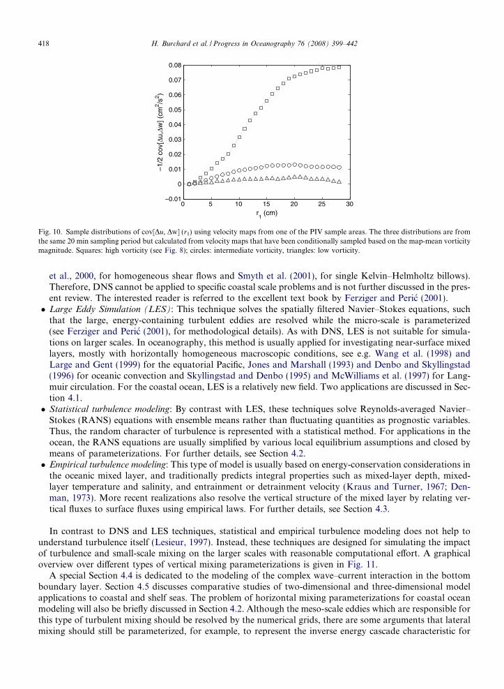
obtained in a vertical plane. Sample distributions of cov[Du, Dw](r1), calculated from velocity maps that havebeen conditionally sampled based on the map-mean vorticity magnitude, are presented in Fig. 10. The valuesof cov[Du, Dw] increase with r1, but converge to constant values as r1 becomes comparable to the integralscale. Performing the calculation across both sample areas would allow for larger integral scales. The condi-tion of r� k is also satisfied (k � 100 m). The conditional sampling clearly shows u0w0 that is substantiallylarger during periods of high vorticity, when the flow contains large vortical structures (Nimmo Smithet al., 2005). Using this approach, PIV data of a vertical plane can be used for obtaining the vertical distribu-tion of u0w0 (Luznik et al., 2007). In the future, stereo PIV could be used to provide the vertical distributions ofall three shear stress components, u0w0, u0v0 and u0w0.

4. Modeling

There are various strategies for modeling turbulence, each of them resolving a different interval of the spec-trum of the flow dynamics:

� Direct Numerical Simulation (DNS): Here, the Navier–Stokes equations which describe all scales of theflow from viscous to global are directly solved by means of discretization techniques. Since all scales inthe ocean are interacting, the viscous scale always needs to be resolved by this technique, and thus, com-putational restrictions limit the method to small scales at relatively low Reynolds numbers (see e.g. Shih

0 5 10 15 20 25 30–0.01

0

0.01

0.02

0.03

0.04

0.05

0.06

0.07

0.08

r1 (cm)

–1/2

cov

[Δu,

Δw] (

cm2 /s

2 )

Fig. 10. Sample distributions of cov[Du, Dw] (r1) using velocity maps from one of the PIV sample areas. The three distributions are fromthe same 20 min sampling period but calculated from velocity maps that have been conditionally sampled based on the map-mean vorticitymagnitude. Squares: high vorticity (see Fig. 8); circles: intermediate vorticity, triangles: low vorticity.


et al., 2000, for homogeneous shear flows and Smyth et al. (2001), for single Kelvin–Helmholtz billows).Therefore, DNS cannot be applied to specific coastal scale problems and is not further discussed in the pres-ent review. The interested reader is referred to the excellent text book by Ferziger and Peric (2001).� Large Eddy Simulation (LES): This technique solves the spatially filtered Navier–Stokes equations, such

that the large, energy-containing turbulent eddies are resolved while the micro-scale is parameterized(see Ferziger and Peric (2001), for methodological details). As with DNS, LES is not suitable for simula-tions on larger scales. In oceanography, this method is usually applied for investigating near-surface mixedlayers, mostly with horizontally homogeneous macroscopic conditions, see e.g. Wang et al. (1998) andLarge and Gent (1999) for the equatorial Pacific, Jones and Marshall (1993) and Denbo and Skyllingstad(1996) for oceanic convection and Skyllingstad and Denbo (1995) and McWilliams et al. (1997) for Lang-muir circulation. For the coastal ocean, LES is a relatively new field. Two applications are discussed in Sec-tion 4.1.� Statistical turbulence modeling: By contrast with LES, these techniques solve Reynolds-averaged Navier–

Stokes (RANS) equations with ensemble means rather than fluctuating quantities as prognostic variables.Thus, the random character of turbulence is represented with a statistical method. For applications in theocean, the RANS equations are usually simplified by various local equilibrium assumptions and closed bymeans of parameterizations. For further details, see Section 4.2.� Empirical turbulence modeling: This type of model is usually based on energy-conservation considerations in

the oceanic mixed layer, and traditionally predicts integral properties such as mixed-layer depth, mixed-layer temperature and salinity, and entrainment or detrainment velocity (Kraus and Turner, 1967; Den-man, 1973). More recent realizations also resolve the vertical structure of the mixed layer by relating ver-tical fluxes to surface fluxes using empirical laws. For further details, see Section 4.3.

In contrast to DNS and LES techniques, statistical and empirical turbulence modeling does not help tounderstand turbulence itself (Lesieur, 1997). Instead, these techniques are designed for simulating the impactof turbulence and small-scale mixing on the larger scales with reasonable computational effort. A graphicaloverview over different types of vertical mixing parameterizations is given in Fig. 11.

A special Section 4.4 is dedicated to the modeling of the complex wave–current interaction in the bottomboundary layer. Section 4.5 discusses comparative studies of two-dimensional and three-dimensional modelapplications to coastal and shelf seas. The problem of horizontal mixing parameterizations for coastal oceanmodeling will also be briefly discussed in Section 4.2. Although the meso-scale eddies which are responsible forthis type of turbulent mixing should be resolved by the numerical grids, there are some arguments that lateralmixing should still be parameterized, for example, to represent the inverse energy cascade characteristic for

Fig. 11. Diagram showing different types and classes of vertical mixing parameterizations. MY: Mellor–Yamada-type models, KPP: K-profile-parameterisation, TKE: Turbulent kinetic energy. This is an extension of a similar diagram designed by Haidvogel and Beckmann(1999).


geostrophic turbulence. In coastal modeling, it is common practice to use a lateral smoothing operator todamp numerical noise.

4.1. Large eddy simulation

Large-eddy simulation (LES) models move beyond approximate techniques by simulating the largest scalesof turbulence using a filtered version of the Navier–Stokes equation. Filtering results in an equation form sim-ilar to Reynolds averaging (see Section 4.2), but with a more complicated term representing scales of motionsmaller than the grid resolution, commonly referred to as subgrid turbulence.

A typical LES equation of motion for the ocean is

oui

ot¼ �uj

oui

oxj� o

oxjhu00i u00j i �

o~poxiþ 2ijkðuj þ us

jÞfk � di3gq0

q0

þ 2ijkusjnk; ð20Þ

where

~p ¼ pq0

þ 2

3q2 þ 1

2½jui þ us

i j2 � juij2�; nk ¼ 2kij

ouj

oxi

� �; ð21Þ

and hu00i u00j i represents the subgrid mixing parameterization. Here, ui are the filtered velocity components, xi arethe Cartesian distances, t is time, g is the acceleration due to gravity, us

j are the Stokes drift components rep-resenting surface waves, fk is the Coriolis term q0, is the perturbation density, q0 is the mean density, p is thepressure, q is the subgrid scale TKE, and 2ijk represents the anti-symmetric tensor. Major differences betweenthe LES momentum equation and the standard Navier–Stokes equations include the Stokes drift term, whichrepresents the effect of surface wave orbital motions on the mean currents, and forces LC, and the subgridterm, which accounts for unresolved turbulence. A wide range of subgrid scale parameterizations exist thatgive excellent results for neutral and convectively forced turbulence. Stable conditions are more problematicbecause the vertical scales of turbulence are reduced and may fall below the grid resolution. In recent years,


methods that use the original filtered velocity stress equation along with dynamic coefficients have led toimprovements for weakly stable turbulence (see Vremen et al., 1997). Nevertheless, very stable conditions thatcause intermittent turbulence remain an unsolved problem. Extensive reviews of LES models are given in Gal-perin and Orzag (1993) and Ferziger and Peric (2001).

Used properly, LES models provide a powerful tool for examining the formation of turbulence and othersmall-scale processes such as LC (for example, see Skyllingstad and Denbo, 1995 or McWilliams et al., 1997).However, LES incurs high computational costs because of grid-size requirements and time-step constraints forsmall scale disturbances. For example, a typical ocean surface boundary layer thickness is about 30 m. Resolv-ing the largest eddy scales, roughly the depth of the boundary layer, requires about 10 grid points, or a gridresolution of 3 m in both the vertical and horizontal directions. By contrast, even the highest resolution regio-nal coastal models tend to be limited to horizontal grid spacing of 0.5–1 km. Although computer power hasbeen steadily increasing, LES is still only useful for domain scales less than about 2 km.

4.1.1. Coastal applications

Applications of LES have largely concentrated on surface boundary layer processes with open ocean con-ditions. These studies have typically used open, radiative bottom boundary conditions to account for the deepocean. Most of the turbulent energy in these simulations comes from surface heat flux, winds and wave forc-ing. Heat flux generates turbulent motions via convection, whereas wind and waves generate turbulencethrough shear production and LC. Use of LES in coastal regions is more limited, even though the processesactive in the surface boundary layer in the open ocean are also important for coastal waters.

In addition to surface-layer mixing, the coastal ocean also contains a bottom boundary layer that is forcedby mean and tidal currents. For a flat, featureless coastal bottom, the lower boundary layer is controlledmostly by shear generated turbulence, much like a neutral ABL. Introduction of obstacles to the flow can leadto a more complicated flow structure, with internal waves and hydraulic jumps (see, for example, Farmer andArmi, 1999; Nash and Moum, 2001). There may also be interaction between the surface boundary layer andthe bottom boundary layer.

Almost all LES model applications use periodic lateral boundaries, to avoid the problem of definition ofturbulence fields outside the model domain. In the coastal environment, the periodicity assumption is prob-ably reasonable for small regions in which the forcing conditions are relatively uniform, and the coastal bot-tom slope is small. With the introduction of topography in the form of isolated obstacles, use of periodicboundaries is equivalent to assuming a series of obstacles.

Two scenarios are presented here, with and without topography and stratification, as examples of how LESmight be used in coastal regions. The first case represents a uniformly mixed, shallow coastal water columnwith both bottom roughness and surface forcing. The model is forced with a wind stress of 0.1 N m�2, anda surface wave field with 30 m wavelength and 1 m significant wave height (for estimating the Stokes driftus). A grid domain of 448 points in the horizontal directions and 40 points in the vertical direction is appliedwith a resolution of 0.5 m.

Cross-section plots (Fig. 12) for this case after 2 h show how coherent structures or LC, produced by thesurface wave–current interaction, dominate the flow. Near-surface horizontal scales of LC are typically smallrelative to the depth of the fluid, but increase rapidly with depth. In the middle of the water column, LC scalesare about 25–50 m, or 2–3 times the layer depth. Overall the flow is very turbulent with rapid exchange ofwater between the surface and bottom.

The introduction of topography and stratification will obviously complicate the dynamics (see, e.g. theobservations by Dewey et al., 2005). In the second example, we examine how a simple two-dimensional ridgeaffects the growth of turbulence in the bottom boundary layer. In this case, the motion is forced by a back-ground current increased from a state of rest over a one-hour period.

The response of stratified flow over an obstacle is determined by a number of non-dimensional parametersthat quantify the behavior of internal waves generated by the flow (Baines, 1995). Most important of theseparameters is probably the internal wave mode number,

K ¼ HNpU

; ð22Þ

Fig. 12. (a) Horizontal cross-section from 5 m depth and (b) vertical cross-section from x = 10 of vertical velocity (m s�1) after 2 h.


where H is the water depth, N is the buoyancy frequency, and U is the velocity across the obstacle. For a givenvelocity and stratification, the value of K tells us what the dominant wave mode will be. For example, whenK = 1.2, we would expect a single vertical wave component, whereas if K = 2.2, then two wave componentswould be forced above the obstacle.

Also important for determining the wave behavior is the scaled obstacle height, Nh/U, which measures theimportance of nonlinear effects. For flow with Nh/U > 0.85, nonlinear effects can cause wave overturning and tur-bulence production. Scaled obstacle width, Na/U, is also critical for determining if the flow will generate a train oflee waves (Na/U � 1–10) or a more hydraulic or hydrostatic flow behavior (Na/U � 10–100) with jump conditions.

Simulations of flow over obstacles in an LES model have only recently been undertaken (see, for example,Calhoun et al., 2001). Here, the LES model used in the flat bottom examples is modified by including topog-raphy through a finite volume approach (Adcroft et al., 1997). Using this technique, bottom obstacles are pro-duced by blocking out flow for all grid points below the bottom. For grid points intersected by the bottomterrain, a finite volume is used with mass balance adjusted to account for the smaller fluid volume passingthrough the grid cell. Advective terms in the equations are also modified by adjusting the flux along the sidesof the grid cell (for details see Skyllingstad and Wijesekera, 2004).

Two simulations with differing K demonstrate how the flow responds to bottom obstacles (Fig. 13). In thefirst case, a flow velocity of 0.32 m s�1 and K value of 1.12 generates a lee wave response with large modula-tions in the pycnocline layer. When the current is reduced to 0.16 m s�1, K increases to 2.24 and a mode twointernal wave system is produced. The bottom boundary layer displays more structure than a flat bottom case,with large variations in bottom boundary layer depth and turbulence intensity. Furthermore, the mode twostructure has altered the pycnocline significantly, generating regions of reduced stratification above theobstacle.

In summary, large-eddy simulation provides a valuable tool for examining basic flow processes that couldhave a large impact on turbulence generation and the coastal circulation. Most notable is the effect of bottom

Fig. 13. Vertical cross-sections of horizontal velocity with mean flow subtracted (shaded) and potential density (contours) for backgroundflow of (a) 0.32 m s�1 and (b) 0.16 m s�1 after 3 h.


topography, which can greatly enhance regions of mixing both on the ocean bottom and in the pycnoclineinterior depending on the internal mode characteristics of the flow and the scale of the obstacle. Simulationssuggest that smaller obstacles have less impact because they are engulfed by the bottom boundary layer andtend to generate dispersive non-hydrostatic waves. Larger obstacles generate a less dispersive internal wavefield, which can become unstable and generate regions of turbulence away from the bottom boundary layer.

Lateral boundaries will require further attention for coastal applications. Typical open boundary modelsset the inflow conditions to be uniform without prescribing perturbations, except for the outward propagationof internal waves. With a turbulent boundary layer, prescribing inflow conditions is very difficult because theflow has to have a balanced set of conditions describing the inflow of a range of eddy scales. One way to getaround this problem is to define a subdomain that is periodic, which then feeds in a balanced turbulent fieldthrough the downstream boundary (Mayor et al., 2002). In its present form, this method requires that internalwave energy be absorbed at the model top, which is unrealistic for many ocean situations. (The original Mayoret al. (2002) application was for atmospheric convection where internal waves are of secondary importance.)

4.2. Statistical turbulence closure models

4.2.1. Basic principles

Almost all macroscopic flow processes can be properly described by the Navier–Stokes equations which area statement of the conservation law for momentum in a viscous fluid on the rotating earth. These equationsare usually simplified by neglecting the direct effect of density differences on momentum (Boussinesq approx-imation), and assuming incompressibility of the flow (e.g. Sander, 1998). The Navier–Stokes equations,together with conservation laws for mass (the continuity equation), heat and salt, form a closed system of vis-cous equations for oceanic dynamics. The turbulent motions in the ocean are fully described by this system ofequations, which requires statistical treatment to extract the mean properties of the large-scale flow.

State variables (such as velocity, pressure and salinity) are decomposed into a fluctuating part and a meanpart. This is the so-called Reynolds decomposition, which needs to fulfil various laws to allow a meaningfulstatistical treatment of the equations. Most obviously, the averaging procedure must not affect averaged quan-tities. The only appropriate procedure is the ensemble average, which is theoretically obtained by averagingover an infinite number of macroscopically identical realizations of the same experiment (see Lesieur, 1997).


The Reynolds-averaged Navier–Stokes (RANS) equations are derived by formal substitution of the Rey-nolds decomposition into the viscous equations, and ensemble-averaging the result. The new set of equationsfor the averaged quantities is formally equivalent to the Navier–Stokes equations, but contains now severalnew, unknown, second moments such as the Reynolds stress u0iu

0j; the turbulent heat flux u0iT

0, and the tur-bulent salt flux u0is0 (where subscripts denote spatial directions). As in earlier sections, primes denote fluctu-ating and overbars averaged quantities. Further transport equations may be derived for these secondmoments, but third moments then appear in the equations. Repetition of this procedure, deriving transportequations for ever higher moments, leads to the Friedmann–Keller series (Keller and Friedmann, 1924). Theseries must be truncated at a certain level and the unknown terms closed by means of parameterizations.Second-moment closures retain the second-moment equations and find empirical expressions for the sec-ond-order pressure–strain correlators such as u0iojp0 and the third moments such as u0iu

0ju0k. For the pres-

sure–strain correlators a plethora of closures may be found in the literature (see e.g. Mellor and Yamada,1974; Launder et al., 1975; Kantha and Clayson, 1994; Canuto et al., 2001, 2002; Cheng et al., 2002; Umlaufand Burchard, 2005).

To reduce the number of transport equations, a drastic step is usually taken at this stage: local equilibriumis assumed for the second moments, which are then described by a linear system of equations. This also elim-inates the third moments. One price for this significant simplification is neglect of any non-local processes suchas counter-gradient fluxes which may occur in convective boundary layers. Furthermore, the effect of theearth’s rotation on turbulent motions is neglected, leading to some inaccuracies for deep oceanic convection.

The final step towards a practical turbulence closure model for geophysical flows is the application of theboundary layer assumption which neglects all horizontal mixing terms (see e.g. Burchard, 2002). The result ofthese closure assumptions is the well-known eddy viscosity principle,

u0w0 ¼ �KMoz�u; v0w0 ¼ �KMoz�v; ð23Þw0T 0 ¼ �KHozT ; w0s0 ¼ �KHozs; ð24Þ

with the eddy diffusivity and KM the eddy diffusivity KH which are calculated as follows:

KM ¼ SMk2

e2S2;

k2

e2N 2

� �k2

e; KH ¼ SH

k2

e2S2;

k2

e2N 2

� �k2

e; ð25Þ

where k is the TKE (not to be confused with the wave number k in Eq. (8)), e is the turbulent dissipation rateand S and N are the shear and buoyancy frequency, respectively. The non-dimensional stability functions SM

and SH are complex nonlinear functions of shear- and buoyancy-related non-dimensional parameters. Here,the eddy diffusivities for heat and salt are set to the same values. For a model with different eddy diffusivities,see Canuto et al. (2002). For a comparative study of various sets of stability functions, see Burchard and Bol-ding (2001) and Umlauf and Burchard (2005). Often, these stability functions are further simplified by a localequilibrium assumption, which allows them to be described as functions of the gradient Richardson numberonly (Galperin et al., 1988; Kantha and Clayson, 1994).

4.2.2. One- and two-equation models

It should be clearly noted here that so far nothing has been said about the calculation of the TKE, k and itsdissipation rate, e. It is an often repeated misunderstanding that particular calculation methods for k and e aredirectly related to particular second-moment closure models. As will be discussed below, it is most importantthat calculation methods for the stability functions and e have to be consistent. The turbulent quantities k ande are related through a turbulent length scale l by the well-known Taylor-scaling,

e ¼ cdk3=2

l; ð26Þ

where cd is an empirical parameter. Given an equation for k, it is in principle possible to use an equation forany non-linear combination of l, k and e to calculate e. Both the TKE equation and the length-scale relatedequation may be either full transport equations or algebraic relations. The latter, while simpler, generally leadto lower accuracy and numerical stability.


Transport equations for k and e can be derived by Reynolds averaging (e.g. Wilcox, 1998). For the TKEequation, closure assumptions have to be made only for the turbulent transport terms,

otk þ ozF ðkÞ ¼ KM S2 � KH N 2 � e; ð27Þ

where the advective transports have been neglected. Vertical turbulent fluxes are denoted by F. The terms onthe right-hand side denote shear production, buoyancy production and dissipation rate, respectively. The clo-sure for production and dissipation terms of the dissipation rate e is not straight-forward. Usually, these termsare based on a normalization of the right-hand side of the TKE equation, as in Rodi (1980). Other length-scalerelated equations follow this principle. There are presently two models with full transport equations of thisform used widely in oceanography: the Mellor and Yamada (1982) model has an equation for kl,

otðklÞ þ ozF ðklÞ ¼ l2

e1KM S2 � e3KH N 2 � 1þ e3

llz

� �2 !

e

" #; ð28Þ

while the k–e model calculates e directly,

oteþ ozF ðeÞþ ¼ celekðKM S2 � ce3KH N 2Þ � ce2

e2

k: ð29Þ

In Eqs. (28) and (29), F is the turbulent flux of kl and e, respectively, and e1, e2, e3, ce1, ce2 and ce3 are empiricalconstants.

Another length-scale related quantity is the turbulence frequency x = e/k used in the k–x model (Wilcox,1988), which has recently been extended for geophysical applications by Umlauf et al. (2003). There is also anew generic two-equation model by Umlauf and Burchard (2003), which uses a transport equation for thequantity kmln, where m and n are non-dimensional exponents.

All empirical parameters occurring in these models must be determined from standard flow situations suchas the logarithmic law of the wall for equilibrium turbulence, free decaying turbulence and homogeneous shearflows. Here, the generic two-equation model has the advantage that it contains two more empirical parame-ters, m and n, which allow more flexibility. The buoyancy-related terms in the length-scale equations can bedetermined from the steady-state Richardson number (which takes a value of about 0.25; see Shih et al., 2000)at which turbulence in homogeneous shear layers should be in equilibrium. Burchard and Baumert (1995) andBaumert and Peters (2001) have shown this for the k–e model and Burchard (2001a) for the kl model. In bothcases, the buoyancy-related parameter depends on the choice for the stability function (e.g. Burchard and Bol-ding, 2001).

In the so-called k models, the length-scale related transport equation is replaced by an algebraic relation-ship for the turbulent length scale (l) using Eq. (26) (e.g. Gaspar et al., 1990; Blanke and Delecluse, 1993;Meier, 2001). The physical complexity of the turbulence approach is not necessarily reduced by such an alge-braic relationship. If the left-hand side of Eq. (29), representing a memory of dissipation in time and the (con-troversial) vertical turbulent transport of dissipation, are neglected, the k–e model in its standard form isphysically equivalent to a k model with appropriately chosen length scales (Meier and Kauker, 2002).

4.2.3. Unresolved processes

As mentioned above, the boundary-layer assumption implies neglect of horizontal mixing processes. This isonly realistic when the horizontal eddy activity is properly resolved by the numerical model. For large-scalemodels, this is not the case, and a number of fairly simple subgridscale parameterizations for horizontal mix-ing have been suggested (e.g. the overview by Haidvogel and Beckmann, 1999).

In the case of coastal ocean models, the meso-scale activity is usually resolved. The size of meso-scale eddiesmay be approximated by the local internal Rossby radius. Fennel et al. (1991) observed Rossby radii between1.3 km and 7 km for the Baltic Sea. This means that typical shelf-sea models with resolutions of 3 km are onlyeddy permitting whereas local coastal models with typically 1 km or less horizontal resolution should be eddyresolving. However, increasing the resolution does not make the eddy closure problem go away but simply


shifts it towards smaller scales, and may even render it more complex as only some effects of geostrophiceddies should be parameterized, to prevent ‘‘double counting”.

Eddy closures are still required in regional and coastal models, not only to represent the unresolvedphysical effects of meso-scale eddies, but also to ensure the numerical stability of the model by preventingenstrophy to build-up at the grid-scale (Roberts and Marshall, 1998). The current practice in coastalmodeling is to employ a Laplacian parameterization based on a high-order scale-selective Laplacian oper-ator and a space/flow-dependent eddy coefficient (Smagorinsky, 1963; Leith, 1968; Semtner and Mintz,1977).

Several processes are not reproduced by the statistical turbulence models and vertical closure assumptionsdescribed in this section. Counter-gradient fluxes are excluded because of the neglect of the transport term inthe heat flux equation (e.g. the discussion by Zilitinkevich et al., 1999). It has been shown by Canuto et al.(1994) that statistical models closed on the level of the third moments can reproduce convective turbulence.Effects of breaking surface waves (see Section 3.2) may be parameterized by surface fluxes of TKE, contrastingwith a wall layer where a zero flux is prescribed (see Craig and Banner, 1994). The Mellor and Yamada (1982)model and the k–e model do not correctly reproduce the vertical structure of the flow in the wave-enhancedlayer below the free surface. Thus, some effort has been made to modify these models, for example, by Bur-chard (2001b) for the k–e model. By contrast with this, the k–x model behaves fairly well under breakingwaves and the generic two-equation model can be directly fitted to observed conditions (see Umlauf and Bur-chard, 2003). LC (see Section 4.1) is not reproduced by these statistical closure models, because of the hydro-static assumption and the neglect of surface wave effects. There are only a few attempts to empirically includethis process in such models, for example, by McWilliams et al. (1997), D’Alessio et al. (1998), Axell (2002),Kantha and Clayson (2004). Finally, the most critical process not reproduced by statistical turbulence modelsis the activity of internal waves and their interaction with turbulence (see Section 2.3). After the Reynoldsdecomposition, internal waves are in principle included in the RANS equations, but later partially excludedby the hydrostatic assumption and the model resolution. Thus far, the representation of internal wave mixingin ocean models has been relatively crude (e.g. Mellor, 1989; Large et al., 1994; Meier, 2001; Axell, 2002; St.Laurent and Garrett, 2002).

4.2.4. Example application

Many of the above-mentioned turbulence closure models have been implemented into the Public Domainwater column model General Ocean Turbulence Model (GOTM) which is published via the internet at http://www.gotm.net (Burchard et al., 1999). GOTM has been applied for simulating various oceanic and limnic sce-narios, one of them being the Liverpool Bay 1999 campaign reported and analyzed by Rippeth et al. (2001).The major process observed at this site was the strain-induced periodic stratification (SIPS), and the modelingchallenge was to see whether two-equation turbulence models are able to reproduce the convective mixinginvolved. For this purpose, Simpson et al. (2002) simulated the Liverpool Bay scenario with a k–e model cou-pled to the second moment closure by Canuto et al. (2002).

For the simulation, a barotropic tide, surface fluxes of heat and momentum, horizontal gradients of tem-perature and salinity (assumed to be constant in time and space) and initial conditions for temperature, salin-ity and momentum had to be prescribed from observations. The simulations showed a slight phase shift fortemperature, salinity and momentum compared with the observations, probably as a result of simplisticassumptions about the horizontal density gradients. Since the focus of the simulations was to evaluate the abil-ity of the model to reproduce turbulence dynamics, the simulated temperature and salinity were relaxed toobservations (Simpson et al., 2002). Fig. 14 shows the resulting temperature, salinity and momentum com-pared with observations. The good agreement between observed and simulated temperature and salinity issurely due to the relaxation, which can be regarded as correcting the advection of these quantities. The sim-ulated velocity components, also agree quite well with the observations.

Fig. 15 shows observed and simulated dissipation rate. Quantitatively and qualitatively, the agreement isquite good. In particular, the tidal asymmetry with strongly enhanced turbulence during flood and suppressedturbulence during ebb is clearly reproduced. This result, which has been obtained without any specific tuning,gives some credibility to statistical turbulence models and their applicability in complex coastal and estuarineflow situations.

http://www.gotm.net

http://www.gotm.net

-30

-25

-20

-15

-10

-5

0

186.8 187.0 187.2 187.4 187.6

-30

-25

-20

-15

-10

-5

0

186.8 187.0 187.2 187.4 187.6

-30

-25

-20

-15

-10

-5

0

186.8 187.0 187.2 187.4 187.6

14.0

14.5

15.0

15.5

16.0

-30

-25

-20

-15

-10

-5

0

186.8 187.0 187.2 187.4 187.6

-30

-25

-20

-15

-10

-5

0

186.8 187.0 187.2 187.4 187.6

-30

-25

-20

-15

-10

-5

0

186.8 187.0 187.2 187.4 187.6

14.0

14.5

15.0

15.5

16.0

-30

-25

-20

-15

-10

-5

0

186.8 187.0 187.2 187.4 187.6

-30

-25

-20

-15

-10

-5

0

186.8 187.0 187.2 187.4 187.6

-30

-25

-20

-15

-10

-5

0

186.8 187.0 187.2 187.4 187.6

32.6

32.8

33.0

33.2

33.4

33.6

-30

-25

-20

-15

-10

-5

0

186.8 187.0 187.2 187.4 187.6

-30

-25

-20

-15

-10

-5

0

186.8 187.0 187.2 187.4 187.6

-30

-25

-20

-15

-10

-5

0

186.8 187.0 187.2 187.4 187.6

32.6

32.8

33.0

33.2

33.4

33.6

-30

-25

-20

-15

-10

-5

0

186.8 187.0 187.2 187.4 187.6

-30

-25

-20

-15

-10

-5

0

186.8 187.0 187.2 187.4 187.6

-30

-25

-20

-15

-10

-5

0

186.8 187.0 187.2 187.4 187.6

-30

-25

-20

-15

-10

-5

0

186.8 187.0 187.2 187.4 187.6

-0.8-0.6-0.4-0.20.00.20.40.60.8

-30

-25

-20

-15

-10

-5

0

186.8 187.0 187.2 187.4 187.6

-30

-25

-20

-15

-10

-5

0

186.8 187.0 187.2 187.4 187.6

-30

-25

-20

-15

-10

-5

0

186.8 187.0 187.2 187.4 187.6

-30

-25

-20

-15

-10

-5

0

186.8 187.0 187.2 187.4 187.6

-0.8-0.6-0.4-0.20.00.20.40.60.8

-30

-25

-20

-15

-10

-5

0

186.8 187.0 187.2 187.4 187.6

-30

-25

-20

-15

-10

-5

0

186.8 187.0 187.2 187.4 187.6

-30

-25

-20

-15

-10

-5

0

186.8 187.0 187.2 187.4 187.6

-30

-25

-20

-15

-10

-5

0

186.8 187.0 187.2 187.4 187.6

-0.4

-0.2

0.0

0.2

0.4

-30

-25

-20

-15

-10

-5

0

186.8 187.0 187.2 187.4 187.6

-30

-25

-20

-15

-10

-5

0

186.8 187.0 187.2 187.4 187.6

-30

-25

-20

-15

-10

-5

0

186.8 187.0 187.2 187.4 187.6

-30

-25

-20

-15

-10

-5

0

186.8 187.0 187.2 187.4 187.6

-0.4

-0.2

0.0

0.2

0.4

Fig. 14. Strain-induced Periodic Stratification (SIPS) in Liverpool Bay. Temperature, T salinity s and velocity components �u and �v fromobservations by Rippeth et al. (2001) (left panels) and simulations with nudging to observed T and s (right panels) for two tidal cycles.Note the complete mixing at high water (after flood) and the significant stratification at low water (after ebb). The u-component of thevelocity is onshore, the v-velocity is offshore. It can be clearly seen in the u-velocity profiles how the ebb profiles are significantly shearedthroughout the water column (due to suppression of turbulence by stable stratification), and how the opposite (small shear in the upperparts of the water column) is seen during flood. This figure has been taken from Burchard (2002).


-30

-25

-20

-15

-10

-5

0

186.8 187.0 187.2 187.4 187.6

-30

-25

-20

-15

-10

-5

0

186.8 187.0 187.2 187.4 187.6

-30

-25

-20

-15

-10

-5

0

186.8 187.0 187.2 187.4 187.6

-8

-7

-6

-5

-4

-3

-30

-25

-20

-15

-10

-5

0

186.8 187.0 187.2 187.4 187.6

-30

-25

-20

-15

-10

-5

0

186.8 187.0 187.2 187.4 187.6

-30

-25

-20

-15

-10

-5

0

186.8 187.0 187.2 187.4 187.6

-8

-7

-6

-5

-4

-3

Fig. 15. Strain-induced Periodical Stratification (SIPS) in Liverpool Bay: turbulent dissipation rate in W kg�1 from observations byRippeth et al. (2001) (left panel) and simulations with nudging to observed temperature and salinity (right panel) for two tidal cycles. Forbetter interpretation, the �6.2 isoline is drawn as a bold line. It can be clearly seen that the high turbulence region (expressed as highdissipation rates) reaches up to the surface during flood and only to about midwater during ebb. This figure has been taken from Burchard(2002).


4.3. Empirical turbulence models

Like the statistical models described in Section 4.2, empirical models for coastal turbulence are based on theRANS equations simplified using the boundary layer approximation. However, the modeling of turbulentfluxes differs dramatically from the closure approach. Instead of approximating the fluxes systematically interms of a Friedman–Keller series, the turbulent formulae are based entirely on empirical knowledge of fluxesin geophysical boundary layers.

The main weakness of the empirical approach is that it is only as good as the observations used to modelthe fluxes. Even if the observations were perfectly accurate, the parameterizations are necessarily based ononly a limited number of particular cases. Thus, the empirical approach demands substantial faith in the gen-erality of geophysical boundary layer physics. (The same could be said of statistical approaches, but the prob-lem is more severe in empirical modeling as the latter, by definition, relies almost entirely on observationalevidence to justify the flux parameterizations.)

This weakness is offset by several advantages. First, the empirical approach facilitates the inclusion of phys-ical processes that are not captured naturally by a truncated Friedman–Keller series (e.g. the non-local fluxesdescribed below). A more practical advantage is that empirical turbulence parameterizations do not requirethe incorporation of additional prognostic variables such as TKE. This results in a substantial saving in bothcomputer memory and processing time.

The earliest empirical models treated the boundary layer as a slab (e.g. Kraus and Turner, 1967; Den-man, 1973), and that assumption is retained in some current models (e.g. Price et al., 1986). Here, we focuson a more recent model that, among other advances, allows boundary layers to assume a more realisticvertical structure. This is the non-local K-profile parameterization (KPP), introduced by Large et al.(1994). The KPP is also distinguished from other empirical models by the inclusion of non-local fluxes.These fluxes are driven by eddies on scales comparable to or larger than the vertical scale over whichthe background shear and stratification change. In the nocturnal surface boundary layer, for example,net surface cooling generates a mean density gradient that is unstable near the surface, nearly zero withinthe mixed layer, and strongly stable in the entrainment zone at the base of the mixed layer. Convectiveplumes carry property fluxes that depend on the net buoyancy change across the mixed layer, and there-fore have little relationship to the local gradient at any particular depth. Such fluxes can be strong even inthe mixed layer interior, where the background gradients are near zero. Parameterization of these fluxesusing the standard gradient-diffusion formalism (e.g. Eqs. (23) and (24) of Section 4.2) is clearlyinappropriate.


4.3.1. The K-profile parameterization

The KPP was described first and in greatest detail by Large et al. (1994). Since then, a number of studieshave led to refinements of the model: Large and Gent (1999), McWilliams and Sullivan (2001), Smyth et al.(2002) and Wijesekera et al. (2003). The reader may find details of the model in any of these publications; here,we will describe only its essential structure.

The KPP treats boundary and interior regions separately. Parameterizations are needed to effect this sep-aration as well as to approximate the fluxes within each region. For simplicity, we describe the parameteriza-tion of fluxes in a surface boundary layer and in the interior region beneath it. Application in coastal regionsdemands the additional consideration of bottom boundary layers, an extension that is straightforward in prin-ciple but more complicated in practice (Durski et al., 2002; Wijesekera et al., 2003).

The boundary layer and the underlying thermocline are separated by the surface z = �h(t). (The verticalcoordinate is positive upwards and zero at the ocean surface). The boundary-layer depth h(t) is defined asthe shallowest depth z at which the bulk Richardson number, Rb(z, t) (see Large et al., 1994), exceeds a spec-ified critical value Ric. The bulk Richardson number is computed in terms of differences in density and hor-izontal velocity between the given depth and the surface layer (defined most simply as the upper tenth of theboundary layer).

The vertical turbulent flux c0w0 of any fluctuating quantity c0 is expressed as the sum of a local and a non-local part, represented as

c0w0 ¼ c0w0L þ c0w0N : ð30Þ
The local component is given by the usual gradient parameterization,
c0w0L ¼ �KcoCoz; ð31Þ

where C(z, t) represents a mean field quantity whose fluctuating part is c0 and Kc(z, t) is the corresponding tur-bulent diffusivity. Parameterization of the diffusivity Kc is described next; non-local fluxes are discussedsubsequently.

Below the boundary layer (z < �h), fluxes are entirely local and are defined using simple parameterizationsof three classes of processes: internal-wave breaking, shear instability and double diffusion. Wave breaking isrepresented by a constant diffusivity that depends only on the quantity represented by c, i.e. momentum or ascalar concentration. The diffusivity due to shear instability is the same for all fields and is represented by asimple function of the local gradient Richardson number. Modifications to the original function of Large et al.(1994) have been described by Large and Gent (1999). Double diffusion is parameterized in terms of the ratio,Rq, of thermal to saline components of the density stratification.

Within the surface boundary layer (z > �h), the diffusivity Kc is parameterized as the product of the bound-ary layer depth, a turbulent velocity scale and a vertical shape function,

Kc ¼ hðtÞ � wcðz; tÞ � Gcðz; tÞ ð32Þ
The velocity scale is proportional to the friction velocity u* and is modified near the surface in accordance withsimilarity scaling. In recent studies (McWilliams and Sullivan, 2001; Smyth et al., 2002), the velocity scale hasbeen modified further to account for mixing by Langmuir cells. The shape function is a cubic function of depthwith coefficients chosen to ensure continuity of fluxes at both the surface and the base of the boundary layer.
The non-local flux of the property c is the flux due to eddies comparable in size to the scale on which thebackground gradient oC=oz varies. Non-local fluxes may be written in terms of local variables by making var-ious approximations to the flux budget (e.g. Deardorff, 1972; Therry and Lacarrere, 1983; Holtzag and Moeng,1991). In low-order models those fluxes must be parameterized in terms of resolved variables. The parameter-ization is contained within an effective ‘‘gradient”, �cc(z, t), that is added to the background gradient of c,

c0w0N ¼ Kccc: ð33Þ

The effective gradient is defined such that the product Kccc depends only on surface fluxes and the surface layerthickness. Large et al. (1994) established parameter values for non-local fluxes of heat and salt. Parameteriza-tion of non-local momentum fluxes has been undertaken more recently by Smyth et al. (2002).


The choice of turbulence closure scheme will depend on the application. For the wave-affected bottomboundary layer, discussed in Section 4.4, early theories were developed using an empirical scheme, but mostrecent studies are moving towards high-resolution statistical schemes. Two cases studies illustrating implemen-tations of the KPP are given in Section 4.5.

4.4. Modeling the wave–current bottom boundary layer

In the coastal ocean, the effects of surface waves may be felt right to the seabed. As already dis-cussed in Section 2.2, the turbulent structure of a wave-induced bottom boundary layer differs signif-icantly from the law of the wall. The presence of the wave-induced boundary layer modifies the thickerboundary layer due to the lower-frequency currents, and thus affects the currents right through thewater column.

There are two common modeling approaches to account for the boundary-layer interaction between high-frequency waves and the mean flow. The first, exemplified by Grant and Madsen (1986), considers the wavemotion as subgrid scale and parameterizes its impact on the mean current field. The second seeks to resolve thewaves’ space and time scales in the numerical model.

4.4.1. The Grant and Madsen approach

Numerous analytical models have been proposed for the structure and interaction of co-existing wave andcurrent boundary layers. The most commonly used models incorporate the influence of the wave boundarylayer in the turbulence parameters of the mean flow, particularly the eddy viscosity and roughness length.This is generally done using a multi-layered approach, where different characteristic turbulent and lengthscales are considered appropriate in different boundary regions. In their classic model, Grant and Madsen(1986) used an empirical, two-layer, time-invariant eddy viscosity, with a wave bottom boundary layerand an overlying wall layer. Both layers have logarithmic current profiles, but with different effective rough-ness lengths. The apparent roughness length for the upper layer is calculated from the requirement of con-tinuous current profiles. This leads to a discontinuity in the eddy viscosity at the top of the wave boundarylayer. The interdependency between the wave- and current-related parameters also requires an iterative solu-tion technique.

Some investigators have proposed less complex eddy viscosity based models that do not require iter-ative solution. Signell et al. (1990) assumed that currents have a negligible effect on the wave boundarylayer. You (1994) reported encouraging comparisons to data when neglecting the angle between wave andcurrent directions, and using a 3-layer eddy viscosity profile similar to Madsen and Wikramanayake(1991).

Most recently, Styles and Glenn (2000) extended the Grant–Madsen model to include water-column strat-ification due to suspended sediment, leading to reduced vertical mixing. The net result of significant strati-fication is an increase in apparent bottom roughness and reductions in bottom shear stress, currents andsediment concentrations. Calculations for typical inner shelf storm conditions showed that their stratificationcorrection ultimately reduced sediment transport rates by almost two orders of magnitude. The possiblerange in values of poorly established model parameters also had an order of magnitude impact on thesepredictions.

The verification of sediment stratification theory is unfortunately problematic. A number of the parametersare difficult to measure and accurate predictions rely heavily upon accurate estimations of physical bed rough-ness and near-bed reference concentration, neither of which is easily determined in its own right. Physical bedroughness is an uncertainty in all wave–current boundary-layer models. If it is calculated from bed shearstress, rather than held constant, one more level of iteration is necessary in the model solution scheme.

Welsh et al. (2001) outline the computational and physics difficulties that can result when bed roughness,wave–current boundary layer and sediment stratification parameterizations are combined to form a multiply-iterative solution scheme. In a related paper, Welsh et al. (2002) present results from Adriatic Sea simulationsusing coupled wave, hydrodynamic and sediment transport models. The effects of the bottom boundary layercouplings include 30% reductions in coastal currents and storm surge, and widespread onset of sediment sus-pension due to wave-dominated forcing in water depths less than 30 m.


4.4.2. High-resolution modeling

Modeling with high vertical resolution has the potential to represent both the wave and turbulence bottom-boundary layers. The advantages of such an approach over analytical boundary layer parameterizationsinclude

� the prediction of boundary layer evolution over a wave cycle and the associated phase lag relationships;� applicability across the continuum from wave-dominated to current-dominated conditions; and� no assumptions regarding steady-state conditions or local turbulence equilibrium.

The time steps and near-bed vertical grid resolutions used in the investigations cited above are on the orderof 0.1 s and 0.1 mm. These levels of resolution are at this time impracticably small for use in three-dimensionalbasin scale or even coastal scale simulations.

Early approaches, usually in 1 or 2 dimensions (e.g. Sheng, 1984; Hagatun and Eidsvik, 1986; Davies et al.,1988), tended to confirm the Grant and Madsen (1986) approach. Most recently, Davies and Villaret (2002)added bed ripple roughness calculations and a related vortex-shedding sub-model to the ‘‘flat bed” model of Liand Davies (1996). These modifications substantially improved agreement with field data for sediment trans-port, confirming the crucial importance of accurate bed roughness estimates. Transport predictions were alsomade using the relatively simple, analytical model of Bijker (1971), with ripple calculations again included.Overall, the TKE model predictions for mean concentration profiles and net longshore sediment transportrates were only slightly better than those of the ‘‘engineering” model. The ability of a numerical model toresolve complex, intra-wave cycle phenomena was again demonstrated through the prediction of cross-shoregrain-size sorting as a consequence of the greater turbulence intensity in the ‘‘wave plus current” half-cycle.

Mellor (2002) carried out one-dimensional simulations of pure wave and wave–current boundary layers,respectively, using TKE and turbulent length scale transport equations. The pure wave boundary layer resultsagreed well at all phases with laboratory data in terms of current profile, shear stress profile, TKE profile andbottom stress. On this basis, the results from the wave–current simulations were used to develop two alterna-tive parameterizations of wave effects for use in large-scale circulation models. The numerical simulations indi-cated that the key impact of waves was an increase in turbulence levels. An additional shear production termwas therefore derived for inclusion in the TKE transport equation. This approach also requires a minor mod-ification of the normal ‘‘law of the wall” boundary condition. For circulation models that do not include aTKE equation, an alternative parameterization for z0a was developed. It is noted, however, that the use ofa z0a approach will unavoidably result in poor mean current predictions very close to the bed (on the orderof a cm).

4.5. Sensitivity of 2D and 3D model results to turbulence parameterizations

In the following subsections, two case studies for coastal and shelf-sea applications are discussed as exam-ples of different turbulence implementations in hydrodynamic models. The first is an application of statisticalturbulence closure to the Baltic Sea, and the second a case of coastal upwelling and downwelling using statis-tical turbulence closures and the KPP-model.

4.5.1. A case study for the Baltic Sea

The Baltic Sea is a large estuary forced by freshwater surplus from river runoff and net precipitation. Thewater exchange with the world ocean is restricted by the narrows and sills of the Danish Straits. In the long-term, high-salinity water from the Kattegat enters the Baltic proper and low-salinity water leaves the estuarydue to the freshwater surplus. A permanent halocline, located deeper than the sills in the entrance area, sep-arates the homogeneous upper layer and the stratified deep water. The direct influence of wind-induced mixingand of convection generated by surface buoyancy fluxes is limited to the upper layer by the strongstratification.

Mixing plays a dominant role in determining both the depth of the seasonal thermocline and the verticalcirculation in the Baltic Sea on annual to decadal time scales, see the recent review by Reissmann et al. (inpress). The inflowing high-salinity water from the Kattegat is modified by mixing in the shallow entrance area


and by entrainment on its path into the Baltic proper, see the observational studies by Sellschopp et al. (2006),Arneborg et al. (2007) and Umlauf et al. (2007).

4.5.1.1. The seasonal cycle of the thermocline. In general, the seasonal thermocline is simulated correctly if mix-ing in the ocean is calculated utilizing one of the turbulence models described in Sections 4.2 and 4.3 (see alsoFig. 16).

In summer, thermocline depths are slightly underestimated. In autumn, the model results show a tendencyto overestimate temperature gradients within the thermocline. Especially during the severe winters 1984/1985,1985/1986 and 1986/1987, the formation of the so-called Baltic winter water with temperatures below the tem-perature of maximum density is underestimated. The performance of the k model with appropriately chosenlength scales and of the standard k–e model (Eqs. (27) and (29)) are almost identical.

4.5.1.2. Decadal variability of the permanent halocline. Fig. 17 shows the time evolution of a vertical salinityprofile in the eastern Gotland Basin (Gotland Deep) for the period 1902–1998. The hydrography at GotlandDeep is representative of the main basin of the Baltic Sea. Shown are three simulations utilizing either the stan-dard k–e model or the k model presented in Section 4.2. In the last experiment the surface wind speed has beenincreased by 30% because only daily sea level pressure and wind fields have been considered.

Results of the two turbulence parameterizations, the standard k–e model (Fig. 17b) and the k model(Fig. 17c), are quite different. The standard k–e model causes significantly underestimated salinity in the lower

a

b

c

Fig. 16. Isotherm depths (in �C) from May 1980 to December 1993 in the western Baltic Sea (Bornholm Deep): (a) observations, (b) k–emodel results Meier (2001), and (c) difference between data and model results.

Fig. 17. Isohaline depths (in psu) in the eastern Gotland Basin: (a) observations, (b) standard k–e model, (c) k model, and (d) k model with30% increased wind speed. Observations are not available for periods covering the world wars. The simulations using a Baltic Sea modelwith a horizontal grid distance of 6 nm are described by Meier and Kauker (2002).


layer, while the k model results in significant overestimates. In both simulations the halocline is much too shal-low, causing a model drift towards higher salinities, especially during the first two decades in all simulations.The agreement between the k model with increased wind speed (Fig. 17d) and observations (Fig. 17a) is sat-


isfactory. Minima of lower layer salinity during the 1920/1930s and during the 1980/1990s and the pro-nounced maximum during the 1950s are simulated correctly. The depth of the halocline and maximumlower-layer salinity during the 1950s are still underestimated, and the surface-layer salinity is somewhat toohigh.

The low vertical mixing in the model may follow from exclusion of unresolved processes such as LC andinternal waves. The modelled flux of energy from the wind into inertial motions may also be biased. The three-hour resolution may cause an underestimation of the energy flux by 20% (D’Asaro, 1985). As the energy fluxto inertial motions is proportional to the fourth power of the wind speed, only the tail of the distribution forhigh wind speeds is important for mixing. A few winter storms may provide all of the energy necessary to dee-pen the surface mixed layer as observed.

4.5.2. Coastal upwelling and downwellingWijesekera et al. (2003) examined the sensitivity of model-produced time-dependent upwelling and down-

welling circulation on the Oregon continental shelf to turbulent closure scheme employed with a two-dimen-sional approximation (variations across-shelf and in depth) using the Princeton Ocean Model (POM;Blumberg and Mellor, 1987). The level 2.5 Mellor–Yamada closure (Mellor and Yamada, 1982; Galperinet al., 1988; Kantha and Clayson, 1994), k–e closure (Rodi, 1987; Burchard et al., 1998), and KPP were usedto evaluate eddy fluxes in the circulation model. The model was forced by idealized, constant wind stress with

100

75

50

25

0

Dep

th (m

)

-0.6

-0.3

0v (m s—1)

26

MYK

26

k—εK

26

KPP

100

75

50

25

0

Dep

th (m

)

-0.0001

0

0.0001w (m s—1)

100

75

50

25

0

Dep

th (m

)

-1e-06

0

1e-06Π (s—1)

0 00 0

100

75

50

25

0

Dep

th (m

)

0

0.005

0.01

^KM (m2 s—1)

100

75

50

25

0

Dep

th (m

)

20 15 10 5 0Distance (km)

0

0.005

0.01^KH (m2 s—1)



Fig. 18. Model results for the upwelling case, illustrated by fields of alongshore velocity v (color contours and white lines) together withdensity rh (black contour lines), vertical velocity w (color contours) together with the stream function for the across-stream flow W (blackcontour lines), potential vorticity P, eddy viscosity KM and eddy diffusivity KH for the Mellor–Yamada (k–kl), k–e and KPP mixingschemes after at day 17. All variables are averaged over an inertial period. The contour intervals are Drh = 0.2 kg m�3; Dv = 0.1 m s�1,DW = 0.1 m2 s�1, where W = 0.4 m2 s�1 is marked with a heavy line. Both k–kl and k–e closures used parameters specified by Kantha andClayson (1994). (Adapted from Wijesekera et al., 2003.)


no surface buoyancy flux. The topography was chosen to approximate the Oregon continental shelf and slopeat latitude 45N. Here, we review results from two cases in which wind forcing was upwelling- and downwel-ling-favorable.

Upwelling case: All three closure schemes produced similar features in the mesoscale circulation includingupwelling near the coast and a southward coastal jet (Fig. 18). The across-shelf circulation pattern shown bythe stream function W illustrates offshore Ekman transport in the surface boundary layer, with onshore trans-port concentrated in the bottom boundary layer. Although the thickness of boundary layers is similar for allthree schemes, the structure within these layers depends upon the submodel.

Downwelling case: Again, all three models produce a similar mesoscale circulation over the shelf (Fig. 19),now including downwelling front, coastal jet and symmetric instabilities (e.g. Allen and Newberger, 1998) inthe bottom boundary layer. The velocity front is sharpest in the k–e model, with k–kl and KPP velocity frontscomparable. Although the velocities are in good agreement for all three schemes, there is a small offshore flowat the surface and onshore flow near the bottom for KPP, which can be seen in W field of Fig. 19. On the inner-part of the shelf, potential density is vertically uniform and surface boundary layer extends to the bottom. Forthe KPP scheme this implies that the mixing coefficients are determined for the full depth by the non-dimensional shape function Gx which results in greater mixing in the interior than in the k–kl and the k–eclosure.

100

75

50

25

0

Dep

th (

m)

00.20.40.60.8

v (m s–1)MYK k–εK KPP

100

75

50

25

0

Dep

th (

m)

-0.0002

0

0.0002w (m s–1)

100

75

50

25

0

Dep

th (

m)

-2e-06

0

2e-06Π (s–1)

0

00

0

00

0

00

100

75

50

25

0

Dep

th (

m)

0

0.02

0.04

^KM (m2 s–1)


100

75

50

25

0

Dep

th (

m)

0

0.02

0.04

^KH (m2 s–1)



Fig. 19. Model results for the downwelling case, illustrated by fields of alongshore velocity v (color contours and white lines) together withdensity rh (black contour lines), vertical velocity w (color contours) together with the stream function for the across-stream flow W (blackcontour lines), potential vorticity P, eddy viscosity KM and eddy diffusivity KH for the Mellor–Yamada (�k–kl), k–e and KPP mixingschemes after at day 17. All variables are averaged over an inertial period. The contour intervals are Drh = 0.2 kg m�3; Dv = 0.1 m s�1,DW = 0.1 m2 s�1, where W = 0 m2 s�1 is marked with a heavy line and W > 0 is dashed. Both k–kl and k–e closures were used parametersspecified by Kantha and Clayson (1994). (Adapted from Wijesekera et al. (2003).)


4.5.3. Case study overview

For the Baltic Sea studies, vertical diffusion of TKE seemed to play an important role, so that localschemes, like Richardson-number-dependent friction (Pacanowski and Philander, 1981), are probably not suf-ficient to parameterize the mixing. It is not possible from this study to decide if a k model with appropriatelychosen length scales or a k–e model approach is superior for the coupling with an circulation model. Moreimportant for the performance are the details of the turbulence model, such as the value of the parameterce3, the choice of the stability functions, and how vertical diffusion of dissipation in the ocean interior isincluded (see also the discussion by Burchard et al., 1998).

The study by Wijesekera et al. (2003) provides one of the few comparisons of the KPP model to statisticalturbulence closures for two- (or three-) dimensional models. In this case, there are no significant differencesbetween the results obtained with the different schemes, although details in structure of the boundary layersvaried. However, further comparisons over a broader range of initial conditions by Durski et al. (2002) foundmarked differences between solutions with the Mellor–Yamada level 2.5 closure and the K-profile parameter-ization in simulations of shallow stratified water. These differences were related to both the capability for TKEto diffuse in the Mellor–Yamada scheme and the arguably more appropriate relationship established betweenvertical mixing and gradient Richardson number of the KPP.

The two examples discussed in this section show that general recommendations on the use of a certain tur-bulence closure model within three-dimensional models cannot be given. For fairly simple situations such asthe dynamics of coastal upwelling and downwelling, differences between empirical and statistical closure mod-els and between various statistical closures are difficult to identify. For more complex situations such as thebalance between stratification and mixing in the Baltic Sea over long time scales and in different regions (nar-row straits versus Baltic proper), the results of three-dimensional models are sensitive to the choice of theembedded turbulence model. This sensitivity might be dependent on the circulation model itself (e.g. grid res-olution), because the simulated vertical velocity shear is the most important source of TKE below the turbu-lence-enhanced surface layer (Meier, 2001).

5. Conclusions

Recent years have seen considerable advances in our ability to understand and quantify turbulent fluxes incoastal seas. The development of new observational methods and modeling techniques has yielded deeperinsight into turbulent phenomena. LC is a case in point. Investigation of Langmuir dynamics has requiredinnovative instrumentation, such as autonomous underwater vehicles (Thorpe et al., 2003b) and surface-track-ing profiling instruments (Gemmrich and Farmer, 1999a), together with new modeling tools such as LES (Sec-tion 4.1 and the citations therein).

Surface and internal waves complicate the measurement and analysis of coastal ocean turbulent fluxes. Forthe interaction of breaking surface waves with near-surface turbulence, different observational techniques yielddifferent results and insights. Surface-tracking instruments resolve thinner near-surface layers than free-risingprofilers or instruments mounted on poles (Section 3.2). As long as consistent observational data sets are miss-ing, the development of mathematical models for the reproduction of near-surface processes will also bedelayed. For example, the model by Craig and Banner (1994) has not yet been significantly improved,although it has raised many questions concerning, for example, whether l scales as 0.4 or as 0.2 times the dis-tance from the surface (Umlauf and Burchard, 2003), the functional approximation of turbulent quantitiessuch as TKE and its dissipation rate, and the thickness of the unresolved layer. The impact of surface wavesin shallow water on the near-bed currents are understood in principle (Section 2.2), but the consequences formean transports of mass and suspended matter and the interaction with the sediment remain partially unre-solved. The Grant and Madsen (1986) model, which is conceptually difficult to couple with turbulence models,has survived for more than two decades until its recent challenge from Mellor (2002).

For the interaction between internal waves and turbulence, the situation is even worse. Internal waves arenot resolved in most models, and their parameterization seems to be complicated by their non-local character:they may be generated far away from the location where they break and produce turbulence. Shelf and coastalseas are more complicated because internal waves are not free, but are forced by tidal straining (Section 2.3).


Usually, modellers use simple ‘‘internal wave” parameterizations (Sections 4.2 and 4.3), the simplest being aprescription of constant background diffusivity.

In situ, two-dimensional PIV is one of the more innovative new tools for measuring turbulent processes(Section 3.4). It is the only method that resolves turbulent motions in more than one spatial dimension. Thiseliminates otherwise speculative assumptions on the anisotropy of turbulence. In situ three-dimensional par-ticle tracking velocimetry (3D-PTV) is under current development (Nimmo Smith, 2008) and allows the mea-surement of three-dimensional distributions of all velocity components within a small sample volume. Theapplicability of in situ particle velocimetry techniques in the coastal ocean is limited by the cost of the instru-mentation and its handling. It is thus important to note that more traditional methods such as freely rising orfalling profilers equipped with shear-probes (Section 3.1) and ADCPs (Section 3.3) have been improved andextended in recent years. Specifically, the application of the variance method to high-resolution ADCP dataallows automatic turbulence observations with moored equipment. Here, the cooperation of the instrumentmanufacturers with the researchers is an essential condition for advance of the methods. A fifth beam on com-mercial ADCPs would, for example, allow observation of TKE without the need for assumptions on turbu-lence anisotropy (Section 3.3).

Statistical turbulence modeling, which advanced rapidly in the 1970s (Section 4.2), has been stronglychallenged during the last decade by the empirical KPP model (Sections 4.3 and 4.5). Empirical modelscan be easily extended to reproduce non-local processes such as free convection. Representing the sameprocesses in statistical models requires retention of higher moments in the Friedman–Keller series, so thatthe models become computationally demanding. The capacity of statistical models to reproduce non-localphenomena has been impressively demonstrated by Canuto et al. (1994). A challenge now is formulationof computationally robust and economic statistical models to reproduce non-local features. The ultimateadvantage of such models over empirical models should be their higher degree of generality, since statis-tical models are based on first principles. Three-dimensional models with relatively complex statistical tur-bulence closure have proliferated in recent years with the growth of computational capability (Section 4.5).It should be noted in this context that the turbulent mixing terms in Ocean General Circulation Modelsare the only terms about which there is a debate. Apart from these terms the models all use similarequations.

Acknowledgements

This article has been written in the framework of the SCOR (Scientific Committee on Oceanic Research)Working Group 111 on Coupling of the Coastal Ocean, Coastal Atmosphere and Wind Waves and Swell.The authors are grateful to Chris Mooers (Miami University, USA) and Norden Huang (National CentralUniversity, Taiwan) for their scientific input within this framework. The authors are further indebted toRose-Marie Vasiljuk (CSIRO, Australia) for her re-editing this text several times. Significant support has alsobeen provided by the US National Science Foundation and the Office of Naval Research, the European Com-munity and the Natural Environment Research Council of the UK.

References

Abarbanel, H.D.I., Holm, D.D., Marsden, J.E., Ratiu, T., 1984. Richardson number criterion for the non linear stability of three-

dimensional stratified flow. Physics Review Letters 52, 2352–2355.

Adcroft, A., Hill, C., Marshall, J., 1997. Representation of topography by shaved cells in a height coordinate ocean model. Monthly

Weather Review 125, 2293–2315.

Adrian, R.J., 1991. Particle-imaging techniques for experimental fluid mechanics. Annual Review of Fluid Mechanics 23, 261–304.

Agrawal, Y.C., Terray, E.A., Donelan, M.A., Hwang, P.A., Williams III, A.J., Drennan, W.M., Kahma, K.K., Kitaigorodskii, S.A., 1992.

Enhanced dissipation of kinetic energy beneath surface waves. Nature 359, 219–220.

Allen, J.S., Newberger, P.A., 1998. On symmetric instabilities in oceanic bottom boundary layers. Journal of Physical Oceanography 28,

1131–1151.

Anis, A., Moum, J.N., 1992. The superadiabatic surface layer of the ocean during convection. Journal of Physical Oceanography 22, 1221–

1227.

Anis, A., Moum, J.N., 1995. Surface wave–turbulence interactions: scaling e(z) near the sea surface. Journal of Physical Oceanography 25,

2025–2045.


Arneborg, L., Fiekas, V., Umlauf, L., Burchard, H., 2007. Gravity current dynamics and entrainment – a process study based on

observations in the Arkona Sea. Journal of Physical Oceanography 37, 2094–2113.

Axell, L., 2002. Wind-driven internal waves and Langmuir circulations in a numerical ocean model of the southern Baltic Sea. Journal of

Geophysical Research 107 (C11), 3204. doi:10.1029/2001JC000922.

Baines, P.G., 1995. Topographic Effects in Stratified Flows. Cambridge University Press, Cambridge.

Baker, M.A., Gibson, C.H., 1987. Sampling turbulence in a stratified ocean: statistical consequences of strong intermittency. Journal of

Physical Oceanography 17, 1817–1837.

Baumert, H., Peters, H., 2001. Second-moment closures and length scales for weakly stratified turbulent shear flows. Journal of

Geophysical Research 105, 6453–6468.

Bijker, E.W., 1971. Longshore transport computations. Journal of Waterway, Port, Coastal, and Ocean Engineering 97, 687–701.

Blanke, B., Delecluse, P., 1993. Variability of the tropical Atlantic Ocean simulated by a general circulation model with two different

mixed layer physics. Journal of Physical Oceanography 23, 1363–1388.

Blumberg, A.F., Mellor, G.L., 1987. A description of a coastal ocean circulation model. In: Heaps, N.S. (Ed.), Three Dimensional Ocean

Models. American Geophysical Union, Washington, DC, pp. 1–16.

Burchard, H., 2001a. Note on the q2l equation by Mellor and Yamada [1982]. Journal of Physical Oceanography 31, 1377–1387.

Burchard, H., 2001b. Simulating the wave-enhanced layer under breaking surface waves with two-equation turbulence models. Journal of


Burchard, H., 2002. Applied Turbulence Modeling in Marine Waters. In: Lecture Notes in Earth Sciences, vol. 100. Springer, Berlin,

Heidelberg, New York.

Burchard, H., Baumert, H., 1995. On the performance of a mixed-layer model based on the k–e turbulence closure. Journal of Geophysical

Research 100, 8523–8540.

Burchard, H., Bolding, K., 2001. Comparative analysis of four second-moment turbulence closure models for the oceanic mixed layer.

Journal of Physical Oceanography 31, 1943–1968.

Burchard, H., Bolding, K., Rippeth, T.P., Stips, A., Simpson, J.H., Sundermann, J., 2002. Microstructure of turbulence in the northern

North Sea: a comparative study of observations and model simulations. Journal of Sea Research 47, 223–238.

Burchard, H., Bolding, K., Villarreal, M.R., 1999. GOTM – a general ocean turbulence model. Theory, Applications and Test Cases.

Technical Report, EUR 18745 EN, European Commission.

Burchard, H., Petersen, O., Rippeth, T.P., 1998. Comparing the performance of the Mellor–Yamada and k–e two-equation closure

models. Journal of Geophysical Research 103, 10543–10554.

Calhoun, R.J., Street, R.L., Koseff, J.R., 2001. Turbulent flow over a wavy surface: stratified case. Journal of Geophysical Research 106,

9295–9310.

Canuto, V.M., Howard, A., Cheng, Y., Dubovikov, M.S., 2001. Ocean turbulence. Part I: one-point closure model – momentum and heat

vertical diffusivities. Journal of Physical Oceanography 31, 1413–1426.

Canuto, V.M., Howard, A., Cheng, Y., Dubovikov, M.S., 2002. Ocean turbulence. Part II: vertical diffusivities of momentum, heat, salt,

mass, and passive scalars. Journal of Physical Oceanography 32, 240–264.

Canuto, V.M., Minotti, F., Ronchi, C., Ypma, M., Zeman, O., 1994. Second-order closure PBL model with new third-order moments:

comparison with LES data. Journal of Atmospheric Science 51, 1605–1618.

Cheng, Y., Canuto, V.M., Howard, A.M., 2002. An improved model for the turbulent PBL. Journal of Atmospheric Sciences 59, 1550–

1565.

Craig, P.D., Banner, M.L., 1994. Modeling wave-enhanced turbulence in the ocean surface layer. Journal of Physical Oceanography 24,

2546–2559.

D’Alessio, S.D.J., Abdella, K., McFarlane, N.A., 1998. A new second-order turbulence closure scheme for modeling the oceanic mixed

layer. Journal of Physical Oceanography 28, 1624–1641.

D’Asaro, E.A., 1985. The energy flux from the wind to near-inertial motions in the surface mixed layer. Journal of Physical Oceanography

15, 1043–1059.

Davies, A.G., Soulsby, R.L., King, H.L., 1988. A numerical model of the combined wave and current bottom boundary layer. Journal of


Davies, A.G., Villaret, C., 2002. Prediction of sand transport rates by waves and currents in the coastal zone. Continental-Shelf Research

22, 2725–2737.

Deardorff, J., 1972. Theoretical expression for the countergradient vertical heat flux. Journal of Geophysical Research 77, 5900–5904.

Denbo, D.W., Skyllingstad, E.D., 1996. An open ocean Large Eddy Simulation model with application to deep convection in the

Greenland Sea. Journal of Geophysical Research 11, 1095–1110.

Denman, K.L., 1973. A time-dependent model of the upper ocean. Journal of Physical Oceanography 3, 173–184.

Dewey, R., Richmond, D., Garrett, C., 2005. Stratified tidal flow over a bump. Journal of Physical Oceanography 35, 1927–1991.

Dong, C., Ou, H.-W., Chen, D., Visbeck, M., 2004. Tidally induced cross-frontal mean circulation: analytical study. Journal of Physical

Oceanography 34, 293–305.

Drennan, W.M., Donelan, M.A., Terray, E.A., Katsaros, K.B., 1996. Oceanic turbulence measurements in SWADE. Journal of Physical


Duncan, J.D., 2001. Spilling breakers. Annual Review of Fluid Mechanics 33, 517–547.

Durski, S.M., Glenn, S.M., Haidvogel, D.B., 2002. Vertical mixing schemes in the coastal ocean: comparison of the Level 2.5 Mellor–

Yamada scheme with an enhanced version of the K-profile parameterization. Journal of Geophysical Research 109, C01015.

doi:10.1029/2002JC001702, 2004.

http://dx.doi.org/10.1029/2001JC000922

http://dx.doi.org/10.1029/2002JC001702,2004


Eriksen, C.C., 1978. Measurements and models of fine structure, internal gravity waves, and wave breaking in the deep ocean. Journal of


Farmer, D.M., Armi, L., 1999. Stratified flow over topography: the role of small scale entrainment and mixing in flow reestablishment.

Proceedings of the Royal Society of London, Series A 455, 3221–3258.

Fennel, W., Seifert, T., Kayser, B., 1991. Rossby radii and phase speeds in the Baltic Sea. Continental-Shelf Research 11, 23–36.

Ferziger, J.H., Peric, M., 2001. Computational Methods for Fluid Mechanics. Springer, Berlin, Heidelberg, New York.

Friedrichs, C.T., 2005. Effects of sediment. In: Baumert, H., Simpson, J.H., Sundermann, J. (Eds.), Marine Turbulence: Theories, Models,

and Observations, Results of the CARTUM Project. Cambridge University Press, Boston, pp. 290–295.

Friedrichs, C.T., Wright, L.D., Kim, S.C., 2000. Bottom-boundary-layer processes associated with fine sediment accumulation in coastal

seas and bays. Continental-Shelf Research 20, 807–841.

Furue, R., 2003. Energy transfer within the small-scale oceanic internal wave spectrum. Journal of Physical Oceanography 33, 267–282.

Galperin, B., Kantha, L.H., Hassid, S., Rosati, A., 1988. A quasi-equilibrium turbulent energy model for geophysical flows. Journal of the

Atmospheric Sciences 45, 55–62.

Galperin, B., Orzag, S.A., 1993. Large Eddy Simulation of Complex Engineering and Geophysical Flows. Cambridge University Press,

Cambridge.

Gargett, A.E., 1984. Vertical eddy diffusivity in the ocean interior. Journal of Marine Research 42, 359–393.

Gargett, A.E., 1999. Velcro measurement of turbulent kinetic energy dissipation rate. Journal of Atmospheric and Oceanic Technology 16,

1973–1993.

Garrett, C.J.R., Munk, W.H., 1972. Space-time scales of internal waves. Geophysical Fluid Dynamics 3, 225–264.

Gaspar, P., Gregoris, Y., Lefevre, J.-M., 1990. A simple eddy kinetic energy model for simulations of the oceanic vertical mixing: tests at

station Papa and long-term upper ocean study site. Journal of Geophysical Research 95, 16,179–16,193.

Gemmrich, J.R., Farmer, D.M., 1999a. Near surface turbulence and thermal structure in a wind driven sea. Journal of Physical


Gemmrich, J.R., Farmer, D.M., 1999b. Observations of the scale and occurrence of breaking surface waves. Journal of Physical


Gemmrich, J.R., Farmer, D.M., 2004. Near-surface turbulence in the presence of breaking waves. Journal of Physical Oceanography 34,

1067–1086.

Gemmrich, J.R., Mudge, T.D., Polonichko, V.D., 1994. On the energy input from wind to surface waves. Journal of Physical


Gerkema, T., 2001. Internal and interfacial tides: beam scattering and local generation of solitary waves. Journal of Marine Research 59,

227–255.

Glenn, S.M., Grant, W.D., 1987. A suspended sediment correction for combined wave and current flows. Journal of Geophysical Research

97, 8244–8264.

Gonella, J., 1972. A rotary-component method for analyzing meteorological and oceanographic vector time series. Deep-Sea Research 19,

833–846.

Grant, W.D., Madsen, O.S., 1986. The continental shelf bottom boundary layer. Annual Review of Fluid Mechanics 18, 265–

305.

Greenan, B.J.W., Oakey, N.S., Dobson, F.W., 2001. Estimates of dissipation in the ocean mixed layer using a quasi-horizontal

microstructure profiler. Journal of Physical Oceanography 31, 992–1004.

Hagatun, K., Eidsvik, K.J., 1986. Oscillating turbulent boundary layers with suspended sediment. Journal of Geophysical Research 91,

13045–13055.

Haidvogel, D.B., Beckmann, A., 1999. Numerical Ocean Circulation Modelling. In: Series on Environmental Science and Management,

vol. 2. Imperial College Press, London.

Heitmann, S., Backhaus, J.O., 2005. Large-eddy simulation of convective shear flows. Deep-Sea Research II 52, 1156–1180.

Hibiya, T., Niwa, Y., Fujiwara, K., 1998. Numerical experiments of non-linear energy transfer within the oceanic internal wave spectrum.

Journal of Geophysical Research 103, 18715–18722.

Hinze, J.O., 1975. Turbulence, second ed. McGraw-Hill, New York.

Holloway, G., 1983. A conjecture relating oceanic internal waves and small-scale processes. Atmosphere–Oceans 21, 107–122.

Holtzag, A.A.M., Moeng, C.-H., 1991. Eddy diffusivity and counter gradient transport in the convective atmospheric boundary layer.

Journal of Atmospheric and Oceanic Technology 48, 1690–1698.

Howard, L.N., 1961. Note on a paper of John W. Miles. Journal of Fluid Mechanics 10, 509–512.

Jensen, B.L., Sumer, B.M., Fredsoe, J., 1989. Turbulent oscillatory boundary layers at high Reynolds numbers. Journal of Fluid

Mechanics 206, 265–297.

Jones, H., Marshall, J., 1993. Convection with rotation in a neutral ocean. Journal of Physical Oceanography 23, 1003–1039.

Kantha, L.H., Clayson, C.A., 1994. An improved mixed layer model for geophysical applications. Journal of Geophysical Research 99,

25235–25266.

Kantha, L.H., Clayson, C.A., 2000. Small Scale Processes in Geophysical Fluid Flows. In: International Geophysics Series, vol. 67.

Academic Press, p. 888.

Kantha, L.H., Clayson, C.A., 2004. On the effect of surface gravity waves on mixing in an oceanic mixed layer. Ocean Modelling 6, 101–

124.

Keller, L., Friedmann, A., 1924. Differentialgleichungen fur die turbulente Bewegung einer kompressiblen Flussigkeit. In: Proceedings of

the First International Congress on Applied Mechanics, Delft, pp. 395–405.


Kemp, P.H., Simons, R.R., 1982. The interaction between waves and currents. Waves propagating with current. Journal of Fluid

Mechanics 116, 227–250.

Kemp, P.H., Simons, R.R., 1983. The interaction between waves and currents. Waves propagating against current. Journal of Fluid

Mechanics 130, 73–89.

Kitaigorodskii, S.A., Donelan, M.A., Lumley, J.L., Terray, E.A., 1983. Wave-turbulence interactions in the upper ocean. Part II. Journal

of Physical Oceanography 13, 1988–1999.

Kocsis, O., Prandke, H., Stips, A., Simon, A., Wuest, A., 1999. Comparison of dissipation of turbulent kinetic energy determined from

shear and temperature microstructure. Journal of Marine Systems 21, 67–84.

Kraus, E.B., Turner, J.S., 1967. A one-dimensional model of the seasonal thermocline, II. The general theory and its consequences. Tellus

19, 98–105.

Kunze, E., 1985. Near-inertial wave propagation in geostrophic shear. Journal of Physical Oceanography 15, 544–565.

Large, W.G., Gent, P.R., 1999. Validation of vertical mixing in an equatorial ocean model using Large Eddy Simulations and

observations. Journal of Physical Oceanography 29, 449–464.

Large, W.G., McWilliams, J.C., Doney, S.C., 1994. Oceanic vertical mixing: a review and a model with a nonlocal boundary layer

parameterization. Reviews of Geophysics 32, 363–403.

Launder, B.E., Reece, G.J., Rodi, W., 1975. Progress in the development of a Reynolds-stress turbulence closure. Journal of Fluid

Mechanics 68, 537–566.

Leith, C.E., 1968. Diffusion approximation for two-dimensional turbulence. Physics of Fluids 10, 1409–1416.

Lesieur, M., 1997. Turbulence in Fluids, third ed. Kluwer Academic, Dordrecht.

Li, M.Z., Davies, A.G., 1996. Towards predicting sediment transport in combined wave–current flow. Journal of Waterway, Port, Coastal,

and Ocean Engineering 122, 157–164.

Li, M., Garrett, C., 1995. Is Langmuir circulation driven by surface waves or surface cooling? Journal of Physical Oceanography 25, 64–

76.

Li, M., Garrett, C., Skyllingstad, E., 2005. A regime diagram for classifying turbulent large eddies in the upper ocean. Deep-Sea Research I

52, 259–278.

Lohrmann, A., Hackett, B., Røed, L.P., 1990. High resolution measurements of turbulence, velocity and stress using a pulse-to-pulse

coherent sonar. Journal of Atmospheric and Oceanic Technology 7, 19–37.

Lorke, A., Wuest, A., 2005. Application of coherent ADCP for turbulence measurements in the bottom boundary layer. Journal of

Atmospheric and Oceanic Technology 22, 1821–1828.

Lu, Y., Lueck, R.G., 1999. Using a broadband ADCP in a tidal channel. Part II: turbulence. Journal of Atmospheric and Oceanic

Technology 16, 1568–1579.

Lueck, R.G., Wolk, F., Yamazaki, H., 2002. Oceanic velocity microstructure measurements in the 20th century. Journal of Oceanography

58, 153–174.

Lumley, J.L., Terray, E.A., 1983. Kinematics of turbulence convected by a random wave field. Journal of Physical Oceanography 13,

2000–2007.

Luznik, L., Gurka, R., Zhu, W., Nimmo Smith, W.A.M., Katz, J., Osborn, T.R., 2007. Distribution of energy spectra, Reynolds stresses,

turbulence production and dissipation in a tidally driven bottom boundary layer. Journal of Physical Oceanography 36, 1527–1550.

Maas, L.R.M., van Haren, J.J.M., 1987. Observations on the vertical structure of tidal and inertial currents in the central North Sea.

Journal of Marine Research 45, 293–318.

Mack, A.P., Hebert, D., 1999. Mixing structure of high-frequency internal waves in the upper eastern equatorial Pacific. Journal of


Macoun, P., Lueck, R., 2004. Modeling the spatial response function of the airfoil shear probe using different sized probes. Journal of

Atmospheric and Ocean Technology 21, 284–297.

Madsen, O.S., Wikramanayake, P.N., 1991. Simple models for turbulent wave–current bottom boundary layer flow. Contract Report

DRP-91-1, US Army Corps of Engineers, Coastal Engineering Research Center, Vicksburg, Mississippi.

Mayor, S.D., Spalart, P.R., Tripoli, G.J., 2002. Application of a perturbation recycling technique in a large-eddy simulation of a mesoscale

convective boundary layer. Journal of Atmospheric and Oceanic Technology 59, 2385–2395.

McWilliams, J.C., Sullivan, P., 2001. Vertical mixing by Langmuir circulations. Spill Science and Technology Bulletin 6, 225–237.

McWilliams, J.C., Sullivan, P.P., Moeng, C.-H., 1997. Langmuir turbulence in the ocean. Journal of Fluid Mechanics 334,

1–30.

Meier, H.E.M., 2001. On the parameterization of mixing in 3D Baltic Sea models. Journal of Geophysical Research 106, 30997–31016.

Meier, H.E.M., Kauker, F., 2002. Simulating Baltic sea climate for the period 1902–1998 with the Rossby Centre coupled ice-ocean model.

Reports in Oceanography, vol. 30. Swedish Meteorological and Hydrological Institute, Norrkoping, Sweden.

Mellor, G.L., 1989. Retrospect on oceanic boundary layer modeling and second moment closure. In: Muller, P., Henderson, D. (Eds.),

Parameterization of Small-scale Processes. Proceedings of the Aha Hulikoa Hawaiian Winter Workshop, Honolulu, University of

Hawaii at Manoa, pp. 251–271.

Mellor, G.L., 2002. Oscillatory bottom boundary layers. Journal of Physical Oceanography 32, 3075–3088.

Mellor, G.L., Yamada, T., 1974. A hierarchy of turbulence closure models for planetary boundary layers. Journal of Atmospheric Sciences

31, 1791–1806.

Mellor, G.L., Yamada, T., 1982. Development of a turbulence closure model for geophysical fluid problems. Reviews of Geophysics 20,

851–875.

Melville, W.K., 1996. The role of surface-wave breaking in air–sea interaction. Annual Review of Fluid Mechanics 26, 279–321.


Miles, J., 1990. Richardson’s number revisited. In: List, E.J., Jirka, G.H. (Eds.), Stratified flows, Proceedings of the Third International

Symposium on Stratified Flows, 3–5 February, 1987, Pasadena, California. American Society of Civil Engineers, pp.

1–7.

Miles, J.W., 1961. On the stability of heterogeneous shear flows. Journal of Fluid Mechanics 10, 496–508.

Moeng, C.-H., Sullivan, P.P., 1994. A comparison of shear and buoyancy-driven planetary boundary layer flow. Journal of Atmospheric

and Oceanic Technology 51, 999–1022.

Mooers, C.N.K., 1975. Several effects of a baroclinic current on the cross-stream propagation of inertial–internal waves. Geophysical

Fluid Dynamics 6, 245–275.

Moum, J.N., Gregg, M.C., Lien, R.C., Carr, M.E., 1995. Comparison of turbulence kinetic energy dissipation rates estimates from two

ocean microstructure profilers. Journal of Atmospheric and Oceanic Technology 12, 346–366.

Muller, P., 1984. Small scale vortical motions. In: Muller, P., Pujalet, R. (Eds.), Proceedings of the 2nd ‘Aha Huliko’ a Hawaiian Winter

Workshop. Hawaii Institute of Geophysics, Honolulu, Hawaii, pp. 249–262.

Munk, W., 1981. Internal waves and small-scale processes. In: Warren, B.A., Wunsch, C. (Eds.), Evolution of Physical Oceanography.

MIT Press, Cambridge, MA, pp. 264–291.

Munk, W., Wunsch, C., 1998. Abyssal recipes II: energetics of tidal and wind mixing. Deep-Sea Research I 45, 1977–2010.

Nash, J.D., Moum, J.N., 2001. Internal hydraulic flows on the continental shelf: high drag states over a small bank. Journal of


Nimmo Smith, W.A.M., 2008. A submersible three-dimensional particle tracking velocimetry system for flow visualization in the coastal

ocean. Limnology and Oceanography: Methods 6, 96–104.

Nimmo Smith, W.A.M., Atsavapranee, P., Katz, J., Osborn, T.R., 2002. PIV measurements in the bottom boundary layer of the coastal

ocean. Experiments in Fluids 33, 962–971.

Nimmo Smith, W.A.M., Katz, J., Osborn, T.R., 2005. On the structure of turbulence in the bottom boundary layer of the coastal ocean.

Journal of Physical Oceanography 35, 72–93.

Nimmo Smith, W.A.M., Osborn, T.R., Katz, J., 2004. PIV measurements in the bottom boundary layer of the coastal ocean. In: Gru, J.,

Liu, P.L.-F., Pedersen, G.K. (Eds.), PIV and Water Waves, Coastal and Ocean Engineering, vol. 9. World Scientific Publishers, pp. 51–

79.

Noh, Y., Fernando, H.J.S., 1991. Dispersion of suspended particles in turbulent flow. Physics of Fluids A 3, 1730–1740.

Oakey, N.S., 1977. An instrument to measure oceanic turbulence and microstructure. Bedford Institute of Oceanography, Report, Ser. B1-

R-77, Dartmouth, Nova Scotia, Canada.

Osborn, T., Farmer, D.M., Vagle, S., Thorpe, S.A., Cure, M., 1992. Measurements of bubble plumes and turbulence from a submarine.

Atmosphere–Oceans 30, 419–440.

Osborn, T.R., 1974. Vertical profiling of velocity microstructure. Journal of Physical Oceanography 4, 109–115.

Osborn, T.R., 1980. Estimates of the local rate of vertical diffusion from dissipation measurements. Journal of Physical Oceanography 10,

83–89.

Pacanowski, R.C., Philander, S.H.G., 1981. Parameterization of vertical mixing in numerical models of the tropical oceans. Journal of


Parsons, J.D., Friedrichs, C.T., Traykovski, P., Mohrig, P., Imran, D., Syvitski, J.P.M., Parker, G., Puig, P., Buttles, J., Garcıa, M.H.,

2007. The mechanics of marine sediment gravity flows. In: Nittrouer, C.A., Austin, J., Field, M., Steckler, M., Syvitski, J., Wiberg, P.

(Eds.), Continental Margin Sedimentation: From Sediment Transport to Sequence Stratigraphy, IAP Special Publication 37.

Blackwell, Oxford, UK, pp. 275–338.

Phillips, O.M., 1971. On spectra measured in an undulating layered medium. Journal of Physical Oceanography 1, 1–6.

Pinkel, R., 1981. Observations of the near-surface internal wave field. Journal of Physical Oceanography 11, 1248–1257.

Pinkel, R., Anderson, S., 1997. Shear, strain, and Richardson number variations in the thermocline. Part I: statistical description. Journal


Prandke, H., 1994. Tests and intercalibrations of an improved airfoil shear probe. Technical Report, April 1994. ME Meerestechnik-

Elektronik GmbH, Trappenkamp.

Prandke, H., Holtsch, K., Stips, A., 2000. MITEC technology development: the microstructure/turbulence measuring system MSS. EUR

19733 EN, European Commission, 2000.

Prandle, D., 1982. The vertical structure of tidal currents. Geophysical and Astrophysical Fluid Dynamics 22, 29–49.

Price, J., Weller, R., Pinkel, R., 1986. Diurnal cycling: observations and models of the upper ocean’s response to diurnal heating, cooling

and wind mixing. Journal of Geophysical Research 91, 8411–8427.

Rascle, N., Ardhuin, F., Terray, E.A., 2006. Drift and mixing under the ocean surface: a coherent one-dimensional description with

application to unstratified conditions. Journal of Geophysical Research 111, C03016. doi:10.1029/2005JC003004.

Reissmann, J., Burchard, H., Feistel, R., Hagen, E., Lass, H.U., Mohrholz, V., Nausch, G., Umlauf, L., Wieczorek, G., in press. State-of-

the-art review on vertical mixing in the Baltic Sea and consequences for eutrophication. Progress in Oceanography.

Richardson, K., Nielsen, T.G., Pedersen, F.B., Heilmann, H.P., Loekkegaard, B., Kaas, H., 1998. Spatial heterogeneity of the planktonic

food web in the North Sea. Marine Ecology Progress Series 168, 197–211.

Rippeth, T.P., 2005. Mixing in seasonally stratified shelf seas. Philosophical Transactions of the Royal Society 363, 2837–2854.

Rippeth, T.P., Palmer, M.R., Simpson, J.H., Fisher, N.R., Sharples, J., 2005. Thermocline mixing in summer stratified continental shelf

seas. Geophysical Research Letters 32, L05602.

Rippeth, T.P., Fisher, N.R., Simpson, J.H., 2001. The semi-diurnal cycle of turbulent dissipation in the presence of tidal straining. Journal


http://dx.doi.org/10.1029/2005JC003004


Rippeth, T.P., Simpson, J.H., Williams, E., Inall, M.E., 2003. Measurement of the rates of production and dissipation of turbulent kinetic

energy in an energetic tidal flow: Red Wharf Bay Revisited. Journal of Physical Oceanography 33, 1889–1901.

Rippeth, T.P., Williams, E., Simpson, J.H., 2002. Reynolds stress and turbulent energy production in a tidal channel. Journal of Physical


Roberts, M., Marshall, D., 1998. Do we require adiabatic dissipation schemes in eddy-resolving ocean models? Journal of Physical


Rodi, W., 1980. Turbulence Models and their Application in Hydraulics. International Association for Hydraulic Research, Delft, The

Netherlands.

Rodi, W., 1987. Examples of calculation methods for flow and mixing in stratified flows. Journal of Geophysical Research 92, 5305–5328.

Sander, J., 1998. Dynamic equations and turbulent closures in geophysics. Continuum Mechanics and Thermodynamics 10, 1–28.

Sellschopp, J., Arneborg, L., Knoll, M., Fiekas, V., Gerdes, F., Burchard, Hans, Lass, H.U., Mohrholz, V., Umlauf, L., 2006. Direct

observations of a medium-intensity inflow into the Baltic Sea. Continental-Shelf Research 26, 2393–2414.

Semtner, A.J., Mintz, Y.H., 1977. Numerical simulation of the Gulf Stream and mid-ocean eddies. Journal of Physical Oceanography 7,

208–230.

Sheng, Y.P., 1984. A turbulent transport model of coastal processes. In: Proceedings of the 19th Coastal Engineering Conference.

American Society of Civil Engineers, Houston, TX, pp. 2380–2396.

Shih, L.H., Koseff, J.R., Ferziger, J.H., Rehmann, C.R., 2000. Scaling and parameterization of stratified homogeneous turbulent shear

flow. Journal of Fluid Mechanics 412, 1–20.

Signell, R.P., Bardsley, R.C., Graber, H.C., Capotondi, A., 1990. Effect of wave–current interaction on wind-driven circulation in narrow,

shallow embayments. Journal of Geophysical Research 95, 9671–9678.

Simpson, J.H., Burchard, H., Fisher, N.R., Rippeth, T.P., 2002. Modeling the cycle of tidal dissipation in a region of tidal straining.

Continental-Shelf Research 22, 1615–1628.

Simpson, J.H., Hughes, D.G., Morris, N.C.G., 1977. The relation of seasonal stratification to tidal mixing on the continental shelf. A

Voyage of Discovery (Deacon 70th Birthday volume). Supplement to Deep-Sea Research, 327–340.

Simpson, J.H., Hunter, J.R., 1974. Fronts in the Irish Sea. Nature 250, 404–406.

Simpson, J.H., Rippeth, T.P., Campbell, A.R., 2000. The phase lag of turbulent dissipation in tidal flow. In: Yanagi, T. (Ed.), Interactions

between Estuaries, Coastal Seas and Shelf Seas. Terra Scientific Publishing, Tokyo, Japan, pp. 57–67.

Simpson, J.H., Rippeth, T.P., Williams, E., Betteridge, K.F.E., 2005. Acoustic Doppler techniques. In: Baumert, H., Simpson, J.H.,

Sundermann, J. (Eds.), Marine Turbulence: Theories, Models, and Observations, Results of the CARTUM Project. Cambridge

University Press, Boston, pp. 127–138.

Skyllingstad, E.D., Denbo, D.W., 1995. An ocean large-eddy simulation of Langmuir circulation in the surface mixed layer. Journal of


Skyllingstad, E.D., Wijesekera, H.W., 2004. Large-eddy simulation of flow over two-dimensional obstacles: high drag states and mixing.

Journal of Physical Oceanography 34 (1), 94–112.

Smagorinsky, J.S., 1963. General circulation experiments with the primitive equations. I: the basic experiment. Monthly Weather Review

91, 99–164.

Smyth, W.D., Moum, J.N., Caldwell, D.R., 2001. The efficiency of mixing in turbulent patches: inferences from direct simulations and

microstructure observations. Journal of Physical Oceanography 31, 1969–1992.

Smyth, W.D., Skyllingstad, E.D., Crawford, G.B., Wijesekera, H., 2002. Nonlocal fluxes and Stokes drift effects in the K-profile

parameterization. Ocean Dynamics 52, 104–115.

Soloviev, A., Lukas, R., 2003. Observation of wave-enhanced turbulence in the near-surface layer of the ocean during TOGA COARE.

Deep-Sea Research I 50, 371–395.

Soloviev, A., Lukas, R., Hacker, P., Schoeberlein, H., Baker, M., Arjannikov, A., 1999. A near-surface microstructure system used during

TOGA COARE: Part II. Journal of Atmospheric and Oceanic Technology 16, 1598–1618.

Soloviev, A., Vershinsky, N.V., Bezverchnii, V.A., 1988. Small-scale turbulence measurements in the surface layer of the ocean. Deep-Sea

Research 35, 1859–1874.

Soulsby, R.L., 1983. The bottom boundary layer of shelf seas. In: Johns, B. (Ed.), Physical Oceanography of Coastal and Shelf Seas.

Elsevier, Amsterdam, pp. 189–266.

Souza, A.J., 2005. Wave–current interaction. In: Baumert, H., Simpson, J.H., Sundermann, J. (Eds.), Marine Turbulence: Theories,

Models, and Observations, Results of the CARTUM Project. Cambridge University Press, Boston, pp. 288–290.

St. Laurent, L., Garrett, C., 2002. The role of internal tides in mixing the deep ocean. Journal of Physical Oceanography 32, 2882–2899.

Stacey, M.T., 1999. Observations of turbulence in a partially stratified estuary. Journal of Physical Oceanography 29, 1950–1970.

Stacey, M.T., Monismith, S.G., Burau, J.R., 1999. Measurements of Reynolds stress profiles in unstratified tidal flow. Journal of


Stewart, R.W., Grant, H.L., 1962. Determining the rate of dissipation of turbulent energy near the surface in the presence of waves.

Journal of Geophysical Research 67, 3176–3180.

Styles, R., Glenn, S.M., 2000. Modeling stratified wave and current bottom boundary layers on the continental shelf. Journal of


Taylor, P.K., 2000. Intercomparison and validation of ocean–atmosphere energy flux fields. Final Report of the Joint WCRP/SCOR

Working Group on Air-Sea Fluxes, WMO/TD-No. 1036, Geneva, Switzerland. <http://www.soc.soton.ac.uk/JRD/MET/WGASF/>.

Terray, E.A., Donelan, M.A., Agrawal, Y.C., Drennan, W.M., Kahma, K.K., Williams, A.J., Hwang, P.A., Kitaigorodskii, S.A., 1996.

Estimates of kinetic energy dissipation under breaking waves. Journal of Physical Oceanography 26, 792–807.

http://www.soc.soton.ac.uk/JRD/MET/WGASF/


Therry, G., Lacarrere, P., 1983. Improving the eddy kinetic energy model for planetary boundary layer description. Boundary Layer

Meteorology 25, 63–88.

Thorpe, S.A., 1995. Dynamical processes of transfer at the sea surface. Progress in Oceanography 35, 315–352.

Thorpe, S.A., Osborn, T.R., Farmer, D.M., Vagle, S., 2003a. Bubble clouds and Langmuir circulation: observations and models. Journal


Thorpe, S.A., Osborn, T.R., Jackson, J.F.E., Hall, A.J., Lueck, R.G., 2003b. Measurements of turbulence in the upper-ocean mixing layer

using Autosub. Journal of Physical Oceanography 33, 122–145.

Trowbridge, J.H., 1998. On a technique for measurement of turbulent shear stress in the presence of surface waves. Journal of

Atmospheric and Oceanic Technology 15, 290–298.

Umlauf, L., Arneborg, L., Burchard, H., Fiekas, V., Lass, H.-U., Mohrholz, V., Prandke, H., 2007. The transverse structure of turbulence

in a rotating gravity current. Geophysical Research Letters 34, L08601. doi:10.1029/2007GL029521.

Umlauf, L., Burchard, H., 2003. A generic length-scale equation for geophysical turbulence models. Journal of Marine Research 61, 235–

265.

Umlauf, L., Burchard, H., 2005. Second-order turbulence closure models for geophysical boundary layers. A review of recent work.

Continental-Shelf Research 25, 795–827.

Umlauf, L., Burchard, H., Hutter, K., 2003. The performance of an extended k–x turbulence model for geophysical flows. Ocean

Modeling 5, 195–218.

van Haren, H., 2003. On the polarization of oscillatory currents in the Bay of Biscay. Journal of Geophysical Research 108 (C9), 3290.

doi:10.1029/2002JC001736.

van Haren, H., Maas, L., Zimmerman, J.T.F., Ridderinkhof, H., Malschaert, H., 1999. Strong inertial currents and marginal internal

wave stability in the central North Sea. Geophysical Research Letters 26, 2993–2999.

Veron, F., Melville, W.K., 1999. Pulse-to-pulse coherent Doppler measurements of waves and turbulence. Journal of Atmospheric and

Oceanic Technology 16, 1580–1597.

Vremen, B., Geurts, B., Kuerten, H., 1997. Large-eddy simulation of the turbulent mixing layer. Journal of Fluid Mechanics 339, 357–390.

Wang, D., McWilliams, J.C., Large, W.G., 1998. Large-eddy simulation of the diurnal cycle of deep equatorial turbulence. Journal of


Welsh, D.J.S., Bedford, K.W., Guo, Y., Sadayappan, P., 2001. Enhancement, evaluation, and application of a coupled wave–current–

sediment model for nearshore and tributary plume predictions. Technical Report ERDC MSRC/PET TR/01-16, US Army Corps of

Engineers, Engineering Research and Development Center, Vicksburg, Mississippi.

Welsh, D.J.S., Bedford, K.W., Guo, Y., Sadayappan, P., 2002. A coupled wave, current, and sediment transport modeling system. In:

Edge, B.L., Hemsley, J.M. (Eds.), Proceedings of the WAVES 2001: The Fourth International Symposium held in San Francisco,

California on 2–6 September, 2001, p. 1880. American Society of Civil Engineers, pp. 1336–1345.

Wijesekera, H.W., Allen, J.S., Newberger, P.A., 2003. Modeling study of turbulent mixing over the continental shelf: comparison of

turbulent closure schemes. Journal of Geophysical Research 108 (C3), 3103. doi:10.1029/2001JC001234.

Wilcox, D.C., 1988. Reassessment of the scale-determining equation for advanced turbulence models. American Institute of Aeronautics

and Astronautics 26, 1299–1310.

Wilcox, D.C., 1998. Turbulence Modeling for CFD. DCW Industries, La Canada, CA.

Wiles, P.J., Rippeth, T.P., Simpson, J.H., Hendricks, P.J., 2006. A novel technique for measuring the rate of turbulent dissipation in the

marine environment. Geophysical Research Letters 33, L21608.

Williams, E., Simpson, J.H., 2004. Uncertainties in estimates of Reynolds stress and TKE production rate using the variance method.

Journal of Atmospheric and Oceanic Technology 21, 347–357.

Winterwerp, J.C., 2001. Stratification effects by cohesive and noncohesive sediment. Journal of Geophysical Research 106, 22559–22574.

Wolk, F., Yamazaki, H., Seuront, L., 2002. A new free-fall profiler for measuring bio-physical microstructure. Journal of Atmospheric

and Oceanic Technology 19, 780–793.

Xing, J., Davies, A.M., 1998. A three-dimensional model of internal tides on the Malin–Hebrides shelf and shelf edge. Journal of


Xing, J., Davies, A.M., 2002. Processes influencing the non-linear interaction between inertial oscillations, near inertial internal waves and

internal tides. Geophysical Research Letters 29 (5). doi:10.1029/2001GL014199.

You, Z.-J., 1994. A simple model for current velocity profiles in combined wave–current flows. Coastal Engineering 23, 289–304.

Zappa, C.J., Asher, W.E., Jessup, A.T., 2001. Microscale wave breaking and air–water gas transfer. Journal of Geophysical Research 106,

9385–9391.

Zilitinkevich, S.S., Gryanik, V.M., Lykossov, V.N., Mironov, D.V., 1999. Third-order transport due to internal waves and non-local

turbulence in the stably stratified surface layer. Journal of Atmospheric Sciences 56, 3463–3477.

http://dx.doi.org/10.1029/2007GL029521

http://dx.doi.org/10.1029/2002JC001736

http://dx.doi.org/10.1029/2001JC001234

http://dx.doi.org/10.1029/2001GL014199

observational and numerical modeling methods for...

Documents