occupation-specific matching efficiency - iabdoku.iab.de/discussionpapers/2016/dp1616.pdf · dialog...

IAB Discussion PaperArticles on labour market issues

16/2016

Katharina DenglerMichael StopsBasha Vicari

ISSN 2195-2663

Occupation-specific matching efficiency

Occupation-specific matching efficiency

Katharina Dengler (IAB)

Michael Stops (IAB)

Basha Vicari (IAB)

Mit der Reihe „IAB-Discussion Paper“ will das Forschungsinstitut der Bundesagentur für Arbeit den

Dialog mit der externen Wissenschaft intensivieren. Durch die rasche Verbreitung von Forschungs-

ergebnissen über das Internet soll noch vor Drucklegung Kritik angeregt und Qualität gesichert

werden.

The “IAB Discussion Paper” is published by the research institute of the German Federal Employ-

ment Agency in order to intensify the dialogue with the scientific community. The prompt publication

of the latest research results via the internet intends to stimulate criticism and to ensure research

quality at an early stage before printing.

IAB-Discussion Paper 16/2016 2

Contents

Contents . . . . . . . . . . . . . . . . . . . . . . . . . . . . . . . . . . . . . . . 3

Abstract . . . . . . . . . . . . . . . . . . . . . . . . . . . . . . . . . . . . . . . 4

Zusammenfassung . . . . . . . . . . . . . . . . . . . . . . . . . . . . . . . . . . 4

1 Introduction . . . . . . . . . . . . . . . . . . . . . . . . . . . . . . . . . . . . 6

2 Literature on occupational standardization and task diversity . . . . . . . . . . . 7

3 Data . . . . . . . . . . . . . . . . . . . . . . . . . . . . . . . . . . . . . . . 8

4 Empirical strategy and results . . . . . . . . . . . . . . . . . . . . . . . . . . . 11

5 Search costs and matching efficiency . . . . . . . . . . . . . . . . . . . . . . . 17

6 Conclusions . . . . . . . . . . . . . . . . . . . . . . . . . . . . . . . . . . . 20

A Appendix . . . . . . . . . . . . . . . . . . . . . . . . . . . . . . . . . . . . . 22

Bibliography . . . . . . . . . . . . . . . . . . . . . . . . . . . . . . . . . . . . . 27


Abstract

Based on rich administrative data from Germany, we address the differences in occupation

specific job-matching processes where an occupation consists of jobs that share extensive

commonalities in their required skills and tasks. These differences can be explained by

the degree of standardization (determined by the existence of certifications or legal reg-

ulations) in an occupation and the diversity of tasks in an occupation. We find that the

matching efficiency improves with higher degrees of standardization and lower task diver-

sity. We discuss the possible mechanisms of these empirical findings in a search theoretic

model: as the standardization of an occupation increases or the diversity of tasks de-

creases, search costs decrease and the optimal search intensity increases. However, the

model reveals that higher search intensities can have positive or negative effects on the

matching efficiency. We discuss the conditions under which the empirical results can be

predicted.

Zusammenfassung

Auf der Grundlage eines umfangreichen administrativen Datensatzes für den deutschen

Arbeitsmarkt untersuchen wir die Unterschiede in berufsspezifischen Matchingprozessen.

Ein Beruf besteht hierbei aus Jobs, die sich durch Gemeinsamkeiten in den erforderlichen

Kenntnissen und Tätigkeiten auszeichnen. Wir zeigen, dass diese Unterschiede durch be-

rufsspezifische Eigenschaften erklärt werden können. Zum einen spielt der Grad der Stan-

dardisierung eines Berufes eine Rolle, der durch das Vorhandensein von Ausbildungsvor-

schriften oder einer gesetzlichen Reglementierung bestimmt wird. Zum anderen kann ein

Einfluss der Diversität der Tätigkeiten, sog. Tasks, in einem Beruf nachgewiesen werden.

Unsere Ergebnisse zeigen, dass die Matchingeffizienz mit einem höheren Grad der Stan-

dardisierung und einer niedrigeren Diversität der Tasks steigt. Die möglichen Mechanis-

men, die unseren Befunden zugrundeliegen, diskutieren wir in einem suchtheoretischen

Modell: mit zunehmenden Grad der Standardisierung und abnehmender Diversität der

Tasks nehmen die Suchkosten ab und die optimale Suchintensität zu. Allerdings ergibt

sich aus dem Modell, dass eine höhere Suchintensität sowohl positive als auch negative

Auswirkungen auf die Matching-Effizienz haben kann. Daher diskutieren wir die Bedingun-

gen, unter denen die empirischen Ergebnisse vorhergesagt werden.

JEL classification: C23, J44, J64

Keywords: search costs, unemployment, vacancies, job matching model, occupa-

tional licensing and certifications, occupational tasks


Acknowledgements: We would like to thank Alexandra Fedorets, Hermann Gartner, Jef-

frey Grogger, Daniel Schnitzlein, Jeffrey Smith, Robert Wright, and various participants at

seminars of the Universities in Hanover, Nuremberg and Regensburg, at the Leibniz Sem-

inar of Berlin Network of Labour Market Researchers (BeNA), at the conference by ZEW

and the German Research Foundation (DFG) on "Occupations, Skills, and the Labour Mar-

ket", the annual meeting of the Scottish Economic Society as well as at the 6th Conference

of the European Survey Research Association (ESRA), Reykjavik, for helpful suggestions.

A special thank goes to Franziska Kugler for excellent research assistance.


1 Introduction

The efficiency of job matching processes determines crucially the extent of unemployment.

Thus, information about the efficiency and its determinants are important for labour market

policy decisions. At the beginning of search and matching processes, firms and workers

fix further aspects of their search behaviour along their expectations to be successful; one

of these aspects is the choice of occupation1 they plan to search in.

Studies showed already that the efficiency of matching processes in occupational labour

markets are quite different due to specific tightening on these markets and due to the dif-

ferent necessary efforts to find a job or a worker, respectively (compare, e.g., Fahr/Sunde,

2004; Stops/Mazzoni, 2010). However, not much is known about the determinants of the

latter differences. We argue that, beside other factors, the extent of labour market trans-

parency is one of these determinants and that occupation-specific properties might influ-

ence it. We consider two occupational properties: firstly, the degree of standardization of

an occupation, which depends on the existence or non-existence of legal regulations or

formal skill requirements to perform a job, and, secondly, the diversity of tasks in an oc-

cupation, which is based on the shares of different types of tasks that individuals have to

perform in these occupations.

We explain why an increase of the degree of an occupation’s standardization reduces the

information asymmetries between a firm and a worker. We define occupations as stan-

dardized when there is a particular corresponding professional qualification with curricula

and/or final examinations that are uniform under federal or state law or bound to legal and

administrative regulations. Such occupations serve as an orientation for actors in the labor

market by providing information about the skills of a potential applicant that would meet

the requirements of a job (Beck/Brater/Daheim, 1980). Thus, as standardized occupations

potentially reduce information asymmetries, the efforts that must be undertaken to obtain

further information about – and to find – these jobs that are worth applying for decrease.

Next, we map a second assumption on the task diversity of an occupation: as the diversity

of tasks increases, the information asymmetries between a firm and a worker increase.

If a job requires high task diversity, a firm must investigate more extensively whether an

applicant is the correct hire. Furthermore, applicants also must exert greater efforts to de-

termine whether a job is suitable.

However, it is hardly possible to observe individual search processes, and relevant analy-

ses in this field are based on macroeconomic matching functions that model the depen-

dency of the number of flows into employment on the number of job seekers and vacancies;

for an overview of the foregoing, compare the surveys of Petrongolo/Pissarides (2001);

Rogerson/Shimer/Wright (2005); Yashiv (2007). We estimate such matching functions,

which also consider matching productivities that differ in occupational labor markets and

are partly explained by occupation-specific properties. Accordingly, we derive the indica-

tors for both occupation-specific properties from the German BERUFENET, an adminis-

trative expert database that contains information that is quite similar to the US O*NET.

The estimations are based on a recent, detailed and high-frequency administrative panel

1 A part of the literature refers to "job titles" instead of the term "occupations". Both terms can be handled assynonyms and should be understood as jobs that share extensive commonalities in their required skills andtasks.


dataset for small regional areas and occupations. We find that matching efficiency in-

creases with the degree of standardization and decreases with the diversity of tasks.

To explain our results, we develop a search theoretic model that is based on the "bulletin

board" matching process model conceived by Hall (1979) and Pissarides (1979). To our

knowledge, we are the first to establish the assumption that the search costs are spe-

cific to the occupation where the search takes place. We enhance that model with two

components involving search costs that are driven by the degree of standardization of an

occupation (which leads to a positive impact on optimal search intensity in terms of the op-

timal number of applications) and the degree of diversity of tasks (which leads to a negative

impact on the optimal search intensity). Moreover, we show that both components influ-

ence the matching efficiency; the plausible reason for this result is that, ceteris paribus,

the matching efficiency is influenced by the optimal search intensity. The model reveals

that a higher search intensity can lead to either positive or negative effects on matching

efficiency: from the employer’s perspective, a higher search intensity leads to a higher

probability of recruiting the right worker(s), whereas from the employee’s perspective, the

job-finding rate decreases as the number of applications on the market increases. Thus,

the theoretically derived effects do not reveal a clear direction, and we instead focus on the

conditions under which the empirical results would be predicted.

The remainder of this paper is organized as follows. In section 2, we give an overview

of the literature on both occupational indicators. In section 3, we describe the data and

the construction of the indicators and provide descriptive statistics. Section 4 includes the

empirical strategy, estimation results and some robustness checks based on alternative

operationalizations of the indicators. In section 5 we discuss our theoretical framework

and the conditions that explain the empirical results. Finally, we summarize our findings in

section 6.

2 Literature on occupational standardization and task diversity

Regarding the indicators for the standardization of an occupation, our analysis refers to the

stream of literature related to occupational licensing. As Kleiner (2006: p.3) notes, this is

a topic that is already quite important as part of the European Economic Policy in the 18th

century and is discussed by Adam Smith’s "Wealth of Nations" (compare, e.g., with Smith,

1990: Book I, Chapter 10, Part II). Smith refers to the effects of occupational licensing on

competition in labor and goods markets, with the result that there are positive wage effects

for employers who offer apprenticeships and grant licenses and somewhat negative effects

for the apprentices on prices, which tend to be higher, and on occupational and regional

mobility, which will become more difficult. The persistence of the positive wage effects in

licensed occupations is demonstrated by Weeden (2002), among others, for the US labor

market and Bol/Weeden (2014) for the European market, while Damelang/Schulz/Vicari

(2015), among others, display empirical evidence of mobility hurdles for standardized or

licensed occupations. Kleiner (2006) also indicates that some of these issues that arise

due to licensing might be avoided by occupational certification.2 Our standardization in-

2 According to Kleiner (2006: p.7), "[...] Licensing is contrasted with certification because, with certification,any person can perform the relevant tasks, but the government or generally another nonprofit agency ad-


dicator is equivalent to either occupational licensing or certification, and we point to an-

other important effect: the contribution of licensing and certification to reducing information

asymmetries between labor supply and labor demand. We suggest that this is part of the

explanation for why people with a license are more likely to be employed, as has recently

been found by Gittleman/Klee/Kleiner (2015).

Regarding the indicator on task diversity, our analysis refers to the tasks within the task-

based approach (TBA) as developed and defined by Autor/Levy/Murnane (2003). Thus far,

tasks have been applied mainly to explain the rising wage inequality in many industrialized

countries by a change of tasks: machines substitute for routine tasks and complement

non-routine tasks. Therefore, the wages of high-skilled and low-skilled individuals increase

relative to the wages of medium-skilled individuals, who are more likely to perform routine

tasks (Autor/Katz/Kearney, 2008; Autor, 2013; Autor/Dorn, 2013). To measure task diver-

sity, we consider the composition of task types for each single occupation and use the

variance of this composition as an indicator of task diversity. Therefore, our paper is also

the first to measure task diversity and to test the effects of task diversity on the matching

efficiency in occupational labor markets.

3 Data

We employ a unique administrative panel dataset for 309 occupational groups in 402

NUTS3 regions with 138 observation periods measured from January 2000 to June 2011.

The occupational groups (3-digit level) are coded based on the German Classification of

Occupations 1988 (KldB 1988). All the data stem from the German Federal Employment

Agency.

We use monthly data regarding stocks, inflows, and outflows of unemployment and reg-

istered vacancies. To obtain unbiased matching parameter estimations, we adjust the

dataset by observations for occupations and NUTS3 regions, respectively, where vacan-

cies, unemployment or flows into employment are zero. This process leads to an unbal-

anced panel data structure with 2,365,080 observations. Table 1 shows some descriptive

statistics for the aggregated stocks and flows from the dataset.

Table 1: Descriptive statistics

Measure Monthly averages 1/2000-6/2011(in 1,000)

Unemployment outflows M 259Unemployment stock U 3,750Registered vacancies stock V 332

Source: Administrative data from the Statistics Department of the Federal Employment Agency 2000-2011.Note: Own calculations of average stocks and flows.

ministers an examination and certifies those who have passed, as well as identifies the level of skill andknowledge for certification.[...]"


To derive occupation-specific properties, we use data from BERUFENET, which is a free

online information portal provided by the German Federal Employment Agency for all oc-

cupations known in Germany that is used mainly for career guidance and job placement.3

Occupational titles are included in BERUFENET if there is a corresponding initial or further

vocational training or degree that is regulated legally or quasi-legally or if an occupational

activity is relevant for the labor market. This holds if the occupational title is used in collec-

tive agreements, if a certain number of employees are working in equivalent jobs or if gen-

erally binding further trainings are available for this occupation. In summary, BERUFENET

includes nearly all occupational titles used in Germany (Matthes/Burkert/Biersack, 2008).

Currently, BERUFENET describes approximately 3,900 single occupations,4 providing a

rich set of occupational information (such as information on the required qualifications and

requirements in an occupational activity, the equipment used, working conditions, potential

specializations or further training, and legal regulations). We use occupations at the 3-digit

level of KldB 1988 to provide both occupation-specific indicators for both standardization

and diversity of tasks.

For the first indicator, we use the operationalization of Vicari (2014): The information

on the standardization of the corresponding professional qualification is available from

BERUFENET under the attribute "Career Group" describing the "entry requirements [of

the occupation] in terms of a required qualification" (Bundesagentur für Arbeit, 2011). In

accordance with the Career Group, the professional qualification of each single occupation

is classified as either requiring a standardized certification or an unstandardized certifica-

tion. Additionally, the attribute "legal regulation", which is also available in BERUFENET, is

used to adjust the standardization of occupations. Legal regulations, such as occupational

licensing, control entry into an occupation by imposing minimum qualification requirements

(Kleiner, 2000; Weeden, 2002). To be able to practice the professional activity of a regu-

lated occupation and to use the specific job title associated with such occupation, proof is

required of a certified professional qualification that is governed by legal and administrative

regulations (Bundesagentur für Arbeit, 2015). This requirement applies to occupations in

which the professional activity must meet specific quality standards to protect the general

public interest, such as medical doctors, lawyers, teachers, etc. To compute the indicator,

Vicari (2014) combines information from the Career Group and legal regulation for the year

2012. We assume that the information from this year is also valid for the observation period

of our data. For our analysis, we employ the indicator aggregated to occupational orders at

the 3-digit level. For the aggregation, each single occupation at the 7-digit level is weighted

with the number of all employees at the 7-digit level divided by the number of employees

at the 3-digit level. This weighting is necessary to ensure that the indicators are driven

by more frequent single occupations within the occupational orders5. This standardization

indicator at the 3-digit level of the KldB 1988 displays an average degree of standardization

of 0.69 (see Table 2).

3 For more information, please visit the BERUFENET homepage:http://berufenet.arbeitsagentur.de/berufe/index.jsp.

4 The single occupations in BERUFENET are classified according to the new German Classification of Oc-cupations 2010 (KldB 2010) and are listed at the lowest possible differentiation level, i.e., the 8-digit level.For the single occupations of KldB 2010, there is an unambiguous conversion table for single occupationsof KldB 1988 at the 7-digit level.

5 See Vicari (2014) for more details on the assignment and calculation.


http://berufenet.arbeitsagentur.de/berufe/index.jsp.

Table 2: Summarizing statistics of the standardization indicator for each occupation i

Indicator Mean Std. Dev. Min MaxDegree of standardization Di 0.69 0.30 0 1

Source: Data from Vicari (2014) on the basis of BERUFENET.Note: Own calculations.

For the second indicator, we use the operationalization of Dengler/Matthes/Paulus (2014).

They follow the extension of the TBA made by Spitz-Oener (2006) for Germany by con-

sidering five task categories: analytical non-routine tasks, interactive non-routine tasks,

cognitive routine tasks, manual routine tasks and manual non-routine tasks. Based on

these five task categories, we can determine the task diversity of an occupation, which is

high if all five task types are required with similar shares and low if, for example, only one

task type is required.

The information on the five task types in each single occupation is available in the so-

called requirement matrix of the expert database BERUFENET, which assigns approxi-

mately 8,000 requirements to single occupations. Dengler/Matthes/Paulus (2014) assign

one of the five task types in an "independent three-coder approach" to each core require-

ment6 and calculate the composition of the five tasks types by dividing the requirements in

each single occupation at the 7-digit level in the respective task type by the total number

of requirements in the single occupation.7 We use this task composition, i.e., the share

of the five task types in each single occupation at the 7-digit level, for the year 2012. We

determine the indicator for the diversity of tasks by calculating the variance of the compo-

sition of the five task types in each single occupation at the 7-digit level and taking 1 minus

this variance. For aggregation of this measure on the 3-digit level, the same weighting

procedure is applied as used for the occupational standardization indicator: each single

occupation at the 7-digit level is weighted with the number of all employees at the 7-digit

level divided by the number of employees at the 3-digit level. This diversity of tasks indi-

cator ranges between 0.84 (low task diversity) and 0.99 (high task diversity). The indicator

tends to increase with the required number of task types. However, the indicator does not

always increase with the required number of task types, as we calculate the variance by

considering the composition of task types in each single occupation. For example, a single

occupation with positive shares in four task types may reveal lower task diversity if some

task types have very low shares compared with a single occupation with positive shares in

three task types.

Table 3 provides descriptive statistics for the average share of task types, as well as for

the indicator diversity of tasks in each occupation at the 3-digit level of the KldB 1988. The

most common task type involves manual non-routine tasks at 27 percent, whereas interac-

tive non-routine tasks show the lowest average share with 8 percent. The resulting average

diversity of tasks is 0.93.

6 In general, the requirement matrix contains requirement groups, additional requirements and core require-ments. The requirement groups specify tools that may be necessary to perform an activity (such as ITprogramming languages). Additional requirements include those that might be important to perform anoccupational activity but that are not mandatory. The authors only consider core requirements that aremandatory requirements to work in the various single occupations.

7 See Dengler/Matthes/Paulus (2014) for more details on the assignment and calculation.


Table 3: Summarizing statistics of the share and the diversity of tasks in each occupation i

Shares Mean Std. Dev. Min MaxAnalytical non-routine tasks 0.19 0.22 0 1Interactive non-routine tasks 0.08 0.15 0 1Cognitive routine tasks 0.24 0.22 0 1Manual non-routine tasks 0.27 0.30 0 1Manual routine tasks 0.22 0.27 0 1

Resulting indicator Mean Std. Dev. Min MaxDiversity of tasks Ei 0.93 0.033 0.84 0.99

Source: Data from Dengler/Matthes/Paulus (2014) on the basis of BERUFENET.Note: Own calculations, the diversity of tasks is based on the variance of shares of task types in each singleoccupation.

4 Empirical strategy and results

We modify the random matching function M = f (U,V), conceived by Pissarides (1979,

1985); Diamond (1982b,a); Mortensen (1982), as specified by a Cobb-Douglas form:

M = AUβU VβV , (1)

where A is the augmented matching productivity. The random matching approach gen-

erally assumes that workers and firms are randomly matched and stem from the pool of

existing unemployed workers and job vacancies.

Following the theoretical model, our analysis refers to an estimation of the parameter A of

the matching function, based on the grade of standardization Di and task complexity Ei in

an occupation i. Thus, the model is modified to

Mi = A(Di, Ei)UβUi VβV

i . (2)

We write A(Di, Ei) as

A(Di, Ei) = exp(δDi) exp(ωEi)C = exp(δDi + ωEi)C. (3)

This implies that if the standardization and the diversity of tasks are zero, augmented

productivity amounts to C because A(0, 0) = C. This constant is adjusted by the two

exponential functions that are driven by the standardization and the diversity of tasks.8 To

summarize, the parameters of interest are δ and ω. We use a logarithmic and augmented

version of equation (2) for the empirical analysis:

log Mi jt = c + δDi + ωEi + βU log Ui jt + βV log Vi jt + γGDPcyc,FS (i),year(t) + µ j + dt + εi jt. (4)

Hereby, log Mi jt denotes the logarithm of the flows from unemployment to employment for

occupation i, region j and observation period t. The variable c is the economy-wide fixed

portion of the augmented matching productivity. The variables log U and log V are the log-

8 Hereby, we assume that high values of standardization or diversity of tasks have a greater influence on theaugmented matching productivity than small values.


arithms of the unemployment and vacancy stocks, whereas βU and βV denote the matching

elasticities of unemployed and vacancies, respectively. The term GDPcyc,FS ( j),year(t) is the

cyclical component of the real gross domestic product for federal state FS in region j and

year t (computed with the Hodrick-Prescott filter Hodrick/Prescott, 1997). This variable is

used as a control for the economic situation. Furthermore, the regression equation con-

tains a regional fixed effects term µ j for each region j that can be interpreted as the local

area’s specific augmented productivity, as well as time fixed effects dt, and an error term ε

for each occupation i, region j and observation period t.Estimation results can be found in Table 4. This table presents model versions OLS 1a –

OLS 4. OLS 1a – OLS 1c correspond to baseline regression equations for a "pure" match-

ing function without the occupation-specific parameters. Model equation OLS 1a contains

only the constant and the logarithms of unemployment and vacancy stocks as explaining

variables. In addition, the equation for OLS 1b includes time and regional fixed effects,

and the equation for OLS 1c contains the cyclical component of the GDP. All further model

versions contain also control variables for the cyclical component of the GDP, the local

area effects and the time fixed effects. We computed Driscoll-Kraay standard errors that

account for general forms of spatial (and temporal dependence) in case of a relative large

time dimension and a quite larger number of cross-sectional units (Driscoll/Kraay, 1998).9

Table 4: Estimation results with log Mi jt as the dependent variable

(1) (2) (3) (4) (5) (6)OLS 1a OLS 1b OLS 1c OLS 2 OLS 3 OLS 4

βU 0.570*** 0.598*** 0.598*** 0.620*** 0.601*** 0.624***(0.007) (0.006) (0.006) (0.006) (0.006) (0.006)

βV 0.117*** 0.129*** 0.128*** 0.114*** 0.132*** 0.118***(0.006) (0.003) (0.003) (0.003) (0.003) (0.003)

δ (Standardization) 0.336*** 0.345***(0.020) (0.020)

ω (Task diversity) -1.098*** -1.319***(0.161) (0.157)

γ(GDPcyc,FS (i),year(t)) 1.173*** 1.294*** 1.169*** 1.292***(0.270) (0.277) (0.270) (0.277)

Constant -0.775*** -1.012*** -1.025*** -1.337*** -0.019 -0.137(0.028) (0.017) (0.018) (0.029) (0.142) (0.127)

Time/area fixed effects x x x x x

Observations 2,365,217 2,365,217 2,365,217 2,365,217 2,365,080 2,365,080Adj. R-squared 0.654 0.707 0.707 0.716 0.708 0.718

Source: Administrative data from the Statistics Department of the Federal Employment Agency 2000-2011.Note: Own calculations, Driscoll-Kraay standard errors are in parentheses.Significance levels: *** p<0.01, ** p<0.05, * p<0.1.

9 We use the procedure conceived by Hoechle (2007) with a default lag length of 4. We do this because,generally, one has to consider cross-sectional dependence in panel data sets like we utilized here. Theconsequence is that (ordinary or even cluster) robust standard errors would be underestimated. However, toget further indications whether cross-sectional dependence has to be considered, we calculated Pesaran’sCD statistic that can be used as a test for cross-sectional dependence in the residuals (Pesaran, 2004).The results reveal that the Null of strong cross-sectional dependence in the residuals cannot be rejected.Details about the computation, the specifications and results are provided on request.


The estimates for the matching elasticities of unemployed and vacancies are comparable

with the estimates from previous studies (compare with Burda/Wyplosz, 1994; Entorf, 1998;

Fahr/Sunde, 2004; Stops/Mazzoni, 2010; Klinger/Rothe, 2012; Stops, 2014). Thus, both

elasticities are significantly positive. The matching elasticities of unemployed are larger

than the matching elasticities of vacancies. Furthermore, the magnitude of the elasticities

does not differ much among all model versions. OLS 2 includes the indicator for standard-

ization, revealing a significantly positive effect on the number of matches. OLS 3 contains

the indicator for the diversity of tasks: the coefficient shows a significant and negative im-

pact on the number of matches. OLS 4 presents the results based on equations including

both indicators, and the results remain robust. Thus, we can conclude that the standard-

ization of an occupation i has a positive effect and the diversity of tasks in an occupation ihas a negative effect on the number of matches for the occupation i.To check the robustness of our results, we use alternative operationalizations of both occu-

pation-specific indicators. The indicator for standardization combines two components of

previous analyses, standardization of corresponding certifications and legal regulations for

entering into an occupation. Both components decrease information asymmetry by provid-

ing information on the knowledge and skills traded between job seekers and employers and

thus decrease search costs. However, the underlying mechanisms differ slightly. On the

one hand, standardized certifications are only implicitly required to practice an occupation,

as they allow the assessment and the comparison of skill bundles among workers. There-

fore, a job seeker with the requested certification will be preferred over one without this

certification. On the other hand, certifications are explicitly required in the case of occupa-

tions that are legally regulated and represent a closing mechanism, as a job seeker without

the requested certification is not allowed to perform the job. Therefore, it is reasonable to

check the robustness of the initial indicator by separately considering both components in

our regression equation. For the considered occupations, the average degree of standard-

ized certifications is 0.64, and the average degree of legal regulation is 0.1 (see upper rows

of Table 5).

Table 5: Summarizing statistics for the alternative indicators

Indicator Mean Std. Dev. Min MaxDegree of standardized certifications Di 0.636 0.32 0 1Degree of legal regulation Di 0.097 0.238 0 1Number of requirements Ei 7.37 3.256 2 20

Source: Data from Vicari (2014) and Dengler/Matthes/Paulus (2014) on the basis of BERUFENET.Note: Own calculations.

Furthermore, we consider the number of requirements that must be performed in an occu-

pation as an alternative for the diversity of tasks indicator by adding the number of require-

ments for each single occupation. Again, for aggregation at the 3-digit level, each single

occupation at the 7-digit level is weighted with the number of all employees at the 7-digit

level divided by the number of employees at the 3-digit level. On average, an occupation

consists of seven requirements that must be performed (see the bottom row of Table 5).


The additional estimation results are presented in Table 6. All regression equations include

control variables for the cyclical component of GDP, the local area effects and the time

fixed effects. Again, we find significant positive coefficients for the standardization indica-

tors and significant negative coefficients for the diversity of tasks indicators. The results

are robust through all model versions (with all conceivable combinations of our 5 indica-

tors, OLS 5 – OLS 20) and thus corroborate our previous findings. We further estimate a

matching function in that constant returns to scale are assumed. Constant returns to scale

(βU + βV = 1 with βU , βV > 0)10 are widely discussed in the literature (compare, e.g., with

Petrongolo/Pissarides, 2001). Dividing equation (1) by the unemployment stock, modifying

it for an occupational property specific matching productivity and taking the logarithm leads

to the estimation equation:

log MRi jt = c + δDi + ωEi + β log θi jt + γGDPcyc,FS (i),year(t) + µ j + dt + εi jt. (5)

Therefore, the matching function in its reduced form consists of the matching rate (number

of matches as the share of unemployment stocks) on the left side. This matching rate is

explained by the ratio of vacancies and unemployment and – as a result – the tightness

of the labor market θ on the right side (with coefficient β = βV ). The main results can be

found in Table 7; further results based on the modified occupation-specific indicators can

be found in Table 9 in the Appendix A. Again, we find a positive influence of the degree

of standardization and a negative influence of the diversity of tasks measures on matching

productivity.11

Though we computed standard errors that are robust to cross-sectional and temporal de-

pendence, our estimates remain highly significant. One reason for this is the enormous

variation in our data set. As a further robustness check, we now conduct the same anal-

yses at a higher aggregation level. We do this because one potential shortcoming of our

detailed data is that there could be measurement errors at the small local area level or

occupational level. In more aggregated data sets, these measurement errors could be

"compensated" for, notwithstanding that the prize are higher standard errors. Thus, we

aggregated the data sets by the occupations over the NUTS3 regions. In the following, we

present specifications without a control for the Gross Domestic Product because we could

only use a variable without regional variation and, therefore, this variable would be redun-

dant considering that we included time fixed effects.12 As expected, the estimates come

with higher standard errors but also higher coefficients of determination (see Table 8, all

further results can be found in the Appendix, Tables 10–12).13 Our results corroborate the

10 Although our results clearly reveal decreasing returns to scale, we perform this exercise as a further oppor-tunity to check the robustness of our results. Technically, we will examine whether the restriction of constantreturns to scale would affect the estimates for the coefficients of the occupation-specific properties.

11 We are aware that in this reduced specification, the magnitude of the coefficients for the diversity of tasksmeasure is approximately two times larger than in the unrestricted specification. Furthermore, the coefficientof determination is much smaller. Our explanation for these results is as follows: decreasing returns toscale, as we found in our unrestricted specification, are expected to reveal a biased estimation of one ormore coefficients in our reduced specification because the estimation equation must be complemented bylog Ui jt and its coefficient that is equal to βU+βV−1. Due to decreasing returns to scale imply βU+βV−1 < 0,omission of log Ui jt leads to a downward-biased estimation of one or more coefficients. This is what we seein the different versions of the reduced specifications.

12 We tested, however, specifications with the GDP variable. It’s coefficients are insignificant in all specifica-tions and the further results hardly changed. The authors provide this results upon request.

13 The results imply that the returns to scale of the matching efficiencies of unemployed and vacancies


Table 6: Further estimation results with log Mi jt as the dependent variable

(1)

(2)

(3)

(4)

(5)

(6)

(7)

(8)

(9)

(10)

(11)

(12)

(13)

(14)

(15)

(16)

OLS

5O

LS6

OLS

7O

LS8

OLS

9O

LS10

OLS

11O

LS12

OLS

13O

LS14

OLS

15O

LS16

OLS

17O

LS18

OLS

19O

LS20

βU

0.62

9***

0.63

0***

0.60

3***

0.60

8***

0.61

9***

0.61

4***

0.61

5***

0.61

9***

0.60

5***

0.62

0***

0.61

8***

0.61

2***

0.62

0***

0.62

8***

0.62

3***

0.63

0***

(0.0

06)

(0.0

06)

(0.0

06)

(0.0

05)

(0.0

05)

(0.0

06)

(0.0

06)

(0.0

06)

(0.0

06)

(0.0

06)

(0.0

06)

(0.0

06)

(0.0

06)

(0.0

06)

(0.0

06)

(0.0

06)

βV

0.11

3***

0.11

6***

0.12

7***

0.11

8***

0.11

4***

0.12

4***

0.12

7***

0.12

2***

0.13

1***

0.12

5***

0.11

7***

0.12

2***

0.12

0***

0.11

2***

0.11

8***

0.11

6***

(0.0

03)

(0.0

03)

(0.0

03)

(0.0

03)

(0.0

03)

(0.0

04)

(0.0

04)

(0.0

04)

(0.0

03)

(0.0

04)

(0.0

03)

(0.0

03)

(0.0

03)

(0.0

03)

(0.0

03)

(0.0

03)

δ(S

tand

ardi

zatio

n)0.

301*

**0.

313*

**(0

.019

)(0

.020

)δ

(Sta

ndar

d.ce

rtifi

cate

s)0.

250*

**0.

294*

**0.

213*

**0.

262*

**0.

228*

**0.

257*

**0.

308*

**0.

275*

**(0

.018

)(0

.019

)(0

.017

)(0

.019

)(0

.019

)(0

.018

)(0

.019

)(0

.019

)δ

(Leg

.re

gula

tion)

0.09

6***

0.21

0***

0.11

0***

0.09

8***

0.11

1***

0.20

6***

0.21

9***

0.21

4***

(0.0

21)

(0.0

20)

(0.0

22)

(0.0

21)

(0.0

22)

(0.0

20)

(0.0

20)

(0.0

20)

ω(T

ask

dive

rsity

)-1

.090

***

-0.7

57**

*-1

.110

***

-0.7

64**

*-1

.366

***

-1.1

09**

*-1

.442

***

-1.1

94**

*(0

.159

)(0

.156

)(0

.158

)(0

.154

)(0

.167

)(0

.172

)(0

.160

)(0

.165

)ω

(Num

ber

ofre

quire

men

ts)

-0.0

12**

*-0

.010

***

-0.0

18**

*-0

.017

***

-0.0

19**

*-0

.017

***

-0.0

13**

*-0

.011

***

-0.0

13**

*-0

.011

***

(0.0

00)

(0.0

00)

(0.0

01)

(0.0

01)

(0.0

01)

(0.0

01)

(0.0

00)

(0.0

01)

(0.0

00)

(0.0

01)

γ(G

DP

cyc,

FS

(i),y

ear(

t))

1.32

4***

1.31

7***

1.19

2***

1.23

3***

1.28

5***

1.23

5***

1.22

8***

1.25

8***

1.18

8***

1.25

1***

1.26

9***

1.23

1***

1.26

2***

1.31

9***

1.28

5***

1.31

3***

(0.2

77)

(0.2

77)

(0.2

70)

(0.2

76)

(0.2

76)

(0.2

72)

(0.2

72)

(0.2

71)

(0.2

70)

(0.2

71)

(0.2

76)

(0.2

76)

(0.2

76)

(0.2

77)

(0.2

77)

(0.2

77)

Con

stan

t-1

.239

***

-0.2

61**

-1.0

49**

*-1

.221

***

-1.3

09**

*-0

.928

***

-0.2

40*

-0.9

54**

*-0

.032

-0.2

60*

-1.1

22**

*0.

021

-0.1

28-1

.210

***

-0.0

01-0

.143

(0.0

27)

(0.1

28)

(0.0

18)

(0.0

25)

(0.0

26)

(0.0

16)

(0.1

37)

(0.0

16)

(0.1

44)

(0.1

39)

(0.0

24)

(0.1

36)

(0.1

39)

(0.0

24)

(0.1

34)

(0.1

37)

Tim

e/ar

eafix

edef

fect

sx

xx

xx

xx

xx

xx

xx

xx

x

Obs

erva

tions

2,36

5,00

22,

365,

002

2,36

5,21

72,

365,

217

2,36

5,21

72,

365,

002

2,36

5,00

22,

365,

002

2,36

5,08

02,

365,

002

2,36

5,00

22,

365,

080

2,36

5,00

22,

365,

002

2,36

5,08

02,

365,

002

Adj

.R

-squ

ared

0.71

80.

719

0.70

80.

713

0.71

60.

711

0.71

20.

712

0.70

90.

712

0.71

50.

715

0.71

60.

717

0.71

70.

718



Table 7: Estimation results with log MRi jt as the dependent variable

(1) (2) (3) (4) (5) (6)OLS 1a OLS 1b OLS 1c OLS 2 OLS 3 OLS 4

θ 0.321*** 0.302*** 0.301*** 0.279*** 0.300*** 0.277***(0.007) (0.005) (0.005) (0.005) (0.005) (0.005)


ω (Task diversity) -2.581*** -2.785***(0.146) (0.137)

γ(GDPcyc,FS (i),year(t)) 1.026*** 1.173*** 1.024*** 1.177***(0.299) (0.304) (0.299) (0.304)

Constant -1.639*** -1.746*** -1.757*** -2.102*** 0.648*** 0.481***(0.033) (0.010) (0.010) (0.026) (0.136) (0.120)

Time/area fixed effects x x x x x

Observations 2,365,217 2,365,217 2,365,217 2,365,217 2,365,080 2,365,080Adj. R-squared 0.291 0.431 0.431 0.452 0.440 0.462


previous findings regarding the direction and significance of the effects of the indicators.

Thus, we can finally conclude from our empirical analysis, throughout all model specifi-

cations and the two different aggregation levels, that the degree of standardization of an

occupation has a positive and the task diversity of an occupation has a negative impact on

the efficiency of job matching.

are nearly constant; therefore, as already discussed, there are smaller differences in the effect estimatesbetween the unrestricted (Table 8 and Table 10 in the Appendix) and the reduced specifications (Tables 11and 12 in the Appendix) for the aggregated data set.


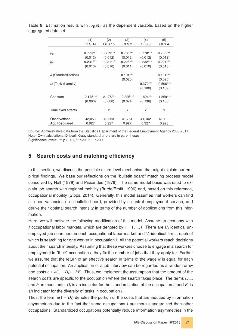
Table 8: Estimation results with log Mit as the dependent variable, based on the higheraggregated data set

(1) (2) (3) (4) (5)OLS 1a OLS 1b OLS 2 OLS 3 OLS 4

βU 0.779*** 0.779*** 0.785*** 0.778*** 0.785***(0.012) (0.012) (0.012) (0.012) (0.012)

βV 0.231*** 0.231*** 0.225*** 0.232*** 0.224***(0.010) (0.010) (0.011) (0.010) (0.010)


ω (Task diversity) -0.372*** -0.506***(0.108) (0.109)

Constant -2.175*** -2.175*** -2.325*** -1.824*** -1.850***(0.060) (0.060) (0.074) (0.136) (0.135)

Time fixed effects x x x x

Observations 42,053 42,053 41,761 41,102 41,102Adj. R-squared 0.927 0.927 0.927 0.927 0.928


5 Search costs and matching efficiency

In this section, we discuss the possible micro-level mechanism that might explain our em-

pirical findings. We base our reflections on the "bulletin board" matching process model

conceived by Hall (1979) and Pissarides (1979). The same model basis was used to ex-

plain job search with regional mobility (Burda/Profit, 1996) and, based on this reference,

occupational mobility (Stops, 2014). Generally, this model assumes that workers can find

all open vacancies on a bulletin board, provided by a central employment service, and

derive their optimal search intensity in terms of the number of applications from this infor-

mation.

Here, we will motivate the following modification of this model: Assume an economy with

I occupational labor markets, which are denoted by i = 1, ..., I. There are Ui identical un-

employed job searchers in each occupational labor market and Vi identical firms, each of

which is searching for one worker in occupation i. All the potential workers reach decisions

about their search intensity. Assuming that these workers choose to engage in a search for

employment in "their" occupation i, they fix the number of jobs that they apply for. Further

we assume that the return of an effective search in terms of the wage w is equal for each

potential occupation. An application or a job interview can be regarded as a random draw

and costs c + a(1 − Di) + bEi. Thus, we implement the assumption that the amount of the

search costs are specific to the occupation where the search takes place. The terms c, a,

and b are constants, Di is an indicator for the standardization of the occupation i, and Ei is

an indicator for the diversity of tasks in occupation i.Thus, the term a(1 − Di) denotes the portion of the costs that are induced by information

asymmetries due to the fact that some occupations i are more standardized than other

occupations. Standardized occupations potentially reduce information asymmetries in the


job search by providing reliable signals about the applicant’s knowledge and skills to meet

the requirements of a job that reduce both individual and firm search costs: The firm knows

whether the applicant is sufficiently qualified for the vacant position, and the applicant

has a clear picture of the requirements and other determinants of the job (Damelang/

Schulz/Vicari, 2015), which implies that as occupations become more standardized, the

amount of effort decreases, that must be made to obtain information about each vacancy

and to find out whether they are worth applying for.

The term bEi denotes the portion of the costs that are induced by information asymmetries

due to the diversity of tasks. If a job offer in occupation i requires a high diversity of tasks,

it is more laborious for a job searcher to explore whether he or she is the right person to

apply for the job. The same is true for a firm that must find out whether the applicant can

perform a lower or higher range of diverse tasks. Thus, we argue that a higher diversity of

tasks leads to higher search costs because of stronger information asymmetries.

The job searchers decide on their search intensities, which can be denoted by their opti-

mal number of job interviews N∗i in occupation i. The probability of obtaining a job after

an interview within occupation i is provided by pi for each occupation i = 1, ..., I. The

job searcher is assumed to maximize the utility of the job search, which is equal to the

difference between the revenue from the job search and the costs of this search:

maxNi{[1 − (1 − pi)Ni]

wr− Ni[c + a(1 − Di) + bEi]}. (6)

In the above equation, [1 − (1 − pi)Ni]w/r denotes the expected revenue to a job searcher

who is currently in occupation i from realizing Ni interviews in occupation i, given pi, the

probability of obtaining a job, and the assumption that a worker cannot hold more than one

job at a given time. We also assume that the expected income from unemployment is zero.

The first-order condition of the optimization problem in (6) is:

− (1 − pi)Ni ln(1 − pi)wr− [c + a(1 − Di) + bEi] = 0 (7)

with the solution:

N∗i =1

ln(1 − pi)ln [−

c + a(1 − Di) + bEiwr ln(1 − pi)

]. (8)

For small pi, we obtain the approximation:

N∗i =

1pi

ln[ (w/r)pic+a(1−Di)+bEi

] for wr pi ≥ [c + a(1 − Di) + bEi],

0 for wr pi < [c + a(1 − Di) + bEi].

(9)

Therefore, optimal job search intensity depends positively on the ratio of the gains to the

costs of a particular job search. A higher wage w has positive effects on job search in-

tensity, whereas higher search costs and higher interest rates have negative effects on

this intensity. The differentiation of the upper case on the right-hand side of equation (9)

with respect to each cost component, the standardization and the diversity of tasks in an

occupation, leads to the equivalent expressions:

∂N∗i∂Di=

1pi

ac+a(1−Di)+bEi

> 0 for wr pi ≥ [c + a(1 − Di) + bEi],

0 for wr pi < [c + a(1 − Di) + bEi].

(10)


∂N∗i∂Ei=

(−1pi

) bc+a(1−Di)+bEi

< 0 for wr pi ≥ [c + a(1 − Di) + bEi],

0 for wr pi < [c + a(1 − Di) + bEi].

(11)

Equations (10) and (11) imply that a higher standardization, Di, has positive effects on the

optimal search intensity, whereas a higher diversity of tasks, Ei, has negative effects on

the optimal search intensity, as long as the expected gain from a job search is larger than

or equal to the search costs. Thus, (w/r)pi ≥ [c + a(1 − Di) + bEi].In the next step of the analysis, the unconditional job-finding probabilities in any occupation

i will be derived from the optimal number of interviews, N∗i . We assume that there is

no information exchange between job searchers. Therefore, it is reasonable that certain

vacancies might attract many applicants whereas other vacancies do not. Furthermore,

we assume that the vacancies in a certain occupation i are all known by at least the job

searchers belonging to that occupation, which compares with the existence of a "bulletin

board" of potential jobs. By defining Ui ≡ Ni∗ui as the sum of applications by unemployed

job searchers in occupation i, we approximately derive the probability that a vacancy in

occupation i will not be considered by the job searchers:

N∗i∏k=1

(1 −1

Vi − k + 1)]ui ≈

N∗i∏k=1

exp(−ui

Vi) = exp (−

Ui

Vi). (12)

The job-finding probability, pi, will be equal to the ratio of the number of vacancies consid-

ered Vi[1− exp(−UiVi

)] to Ui, the number of applications that were submitted by unemployed

workers:

pi =Vi

Ui[1 − exp(−

Ui

Vi)]. (13)

Finally, a matching function that returns the number of flows from unemployment to em-

ployment in an occupation i can be formulated as follows:

Mi(ui, vi) = uiPi = ui[1 − (1 − pi)N∗i ]. (14)

In the equation above, Pi represents the probability that a job searcher in occupation i will

receive at least one job offer. This probability is equal to 1 minus the probability of receiving

no job offer from all the vacancies in occupation i.The matching function above relates exits from unemployment to employment in a certain

occupation to the labor market situation in every occupation. From an empirical perspec-

tive, a problem arises, namely, the optimal search intensity and the search costs cannot

be directly observed. To address this issue, this matching function could be formulated as

a quasi-reduced form that regards vacancies (as well as wages and interest rates, resp.)

as given quantities. This approach renders it possible to study the effects of variations in

portions of the search costs on the number of matches:

∂Mi

∂Di=∂Mi

∂N∗i

∂N∗i∂Di

(15)

=N∗i (1 − pi)−1ui(1 − pi)N∗i∂pi

∂N∗i

∂N∗i∂Di︸︷︷︸

<0

− ln(1 − pi)ui(1 − pi)N∗i∂N∗i∂Di︸︷︷︸

>0

,


∂Mi

∂Ei=∂Mi

∂N∗i

∂N∗i∂Ei

(16)

=N∗i (1 − pi)−1ui(1 − pi)N∗i∂pi

∂N∗i

∂N∗i∂Ei︸︷︷︸

>0

− ln(1 − pi)ui(1 − pi)N∗i∂N∗i∂Ei︸︷︷︸

<0

.

Each of the terms in the equations (15) and (16) reveal contrary effects. There is a positive

(or negative) effect of search intensity on the number of matches given that the job finding

probability would not change, see the last term in equation (15) (or equation (16), resp.) but

there is also an indirect effect because the search intensity influences also the job finding

probability, ∂pi∂N∗i

, in the first term:

∂pi

∂N∗i=

1N∗i

[exp−UiVi (1 +

Vi

Ui) −

Vi

Ui]. (17)

It can be shown that ∂pi∂N∗i

< 0 for all N∗i and UiVi

(with 0 ≤ UiVi≤ ui).

Because we found that∂N∗i∂Di

> 0, the sign of the last term in equation (15) is positive and due

to∂N∗i∂Ei

< 0, the sign of the last term in equation (16) is negative. Considering the conditions

above, the first term would be smaller than zero in equation (15) and larger than zero in

(16). This would imply that the signs of ∂Mi∂Di

and ∂Mi∂Ei

, respectively, depend on the relation

of the first and the last terms.

We can conclude from our model that occupation-specific properties, including the degree

of standardization and the degree of task diversity, might have an important impact on

the intensity with which a worker searches for jobs. However, the direction of the effects

for matching elasticity can be positive or negative. On the one hand, a higher search

intensity tends to lead directly to more matches because workers contact more firms; on

the other hand, a worker’s probability of finding a job decreases due to the intensified

competition among workers. However, our model delivers an explanation regarding the

mechanisms behind our empirical observations. In case the direct positive influence of the

search intensity on the number of matches overcompensates the eventual negative effect

on the job finding probability, our empirical results, ∂Mi∂Di

> 0 and ∂Mi∂Ei

< 0, are predicted by

the model.

6 Conclusions

We discuss implications of two well identifiable occupation-specific properties: the degree

of standardization and the diversity of tasks in an occupation. In particular, these indicators

might have an influence on job or workers search, respectively, and job matching. During

search, firms and workers spend resources such as money and time to provide informa-

tion about themselves and to collect information about one another. In economic terms,

they make efforts to reduce information asymmetries. Information asymmetries determine,

among other factors, the search costs and, given the returns of the search, the optimal

search intensity. Standard job and matching models assume constant search costs for the

entire economy. This assumption is affected by several empirical results that show that the

efficiency of matching firms and workers is quite different in different occupational labor


markets, which are defined as having jobs that share extensive commonalities in their re-

quired skills and tasks. To date, there is not much known about the determinants of these

differences. It is reasonable to assume that both occupation-specific properties might de-

termine information asymmetries and, therefore, the costs of search, as well as – finally –

the observed matching efficiency. We empirically validate the relationship between these

indicators and matching efficiency based on rich administrative data for the period from

2000 to 2011. We find that the degree of standardization exerts a positive influence on the

matching efficiency and that the diversity of tasks exerts a negative influence. The results

are robust to variations in the indicators. We discuss the search mechanisms behind these

findings in a search theoretic model: as the degree of standardization increases and the

task diversity of an occupation decreases, ceteris paribus, the search costs in these oc-

cupations decrease and the search intensity per observation period increases. Firstly, this

can lead to more matches per observation period because a higher number of applications

would lead to a higher probability that each firm is reached by applications and can recruit

a worker. Secondly, the probability that workers will find a job decreases, which would

produce a negative effect on the number of matches. However, we can show that our

empirical observations are predicted by the model under the condition that the first effect

overcompensates the second effect.

Finally, our results suggest that both occupational specific indicators contribute to the ex-

tent of labour market transparency. However, regarding policy decisions for regulations for

vocational training standards or market accesses, the positive implications on job matching

should obviously be weighed up against bureaucratic costs or potentially less flexibility.


A Appendix


Table 9: Further estimation results with log MRi jt as the dependent variable

(1)

(2)

(3)

(4)

(5)

(6)

(7)

(8)

(9)

(10)

(11)

(12)

(13)

(14)

(15)

(16)

OLS

5O

LS6

OLS

7O

LS8

OLS

9O

LS10

OLS

11O

LS12

OLS

13O

LS14

OLS

15O

LS16

OLS

17O

LS18

OLS

19O

LS20

θ0.

268*

**0.

269*

**0.

294*

**0.

291*

**0.

278*

**0.

283*

**0.

284*

**0.

275*

**0.

294*

**0.

276*

**0.

278*

**0.

289*

**0.

279*

**0.

266*

**0.

276*

**0.

266*

**(0

.005

)(0

.004

)(0

.004

)(0

.005

)(0

.004

)(0

.005

)(0

.005

)(0

.005

)(0

.004

)(0

.005

)(0

.005

)(0

.005

)(0

.005

)(0

.004

)(0

.004

)(0

.004

)

δ(S

tand

ardi

zatio

n)0.

329*

**0.

354*

**(0

.022

)(0

.022

)δ

(Sta

ndar

d.ce

rtifi

cate

s)0.

248*

**0.

319*

**0.

177*

**0.

273*

**0.

210*

**0.

247*

**0.

347*

**0.

284*

**(0

.022

)(0

.023

)(0

.020

)(0

.022

)(0

.021

)(0

.021

)(0

.023

)(0

.022

)δ

(Leg

.re

gula

tion)

0.22

0***

0.34

3***

0.23

4***

0.21

8***

0.23

1***

0.32

7***

0.35

1***

0.33

7***

(0.0

24)

(0.0

23)

(0.0

24)

(0.0

24)

(0.0

24)

(0.0

22)

(0.0

22)

(0.0

22)

ω(T

ask

dive

rsity

)-2

.342

***

-1.9

91**

*-2

.572

***

-1.9

70**

*-2

.853

***

-2.3

23**

*-2

.912

***

-2.4

09**

*(0

.135

)(0

.136

)(0

.146

)(0

.137

)(0

.152

)(0

.152

)(0

.144

)(0

.144

)ω

(Num

ber

ofre

quire

men

ts)

-0.0

23**

*-0

.018

***

-0.0

29**

*-0

.026

***

-0.0

30**

*-0

.026

***

-0.0

25**

*-0

.021

***

-0.0

24**

*-0

.019

***

(0.0

01)

(0.0

00)

(0.0

01)

(0.0

01)

(0.0

01)

(0.0

01)

(0.0

01)

(0.0

01)

(0.0

01)

(0.0

00)

γ(G

DP

cyc,

FS

(i),y

ear(

t))

1.23

3***

1.22

4***

1.07

3***

1.08

6***

1.17

6***

1.13

5***

1.12

1***

1.18

7***

1.07

0***

1.17

2***

1.16

2***

1.08

9***

1.15

1***

1.24

5***

1.18

1***

1.23

6***

(0.3

05)

(0.3

04)

(0.2

98)

(0.3

04)

(0.3

03)

(0.3

00)

(0.2

99)

(0.2

98)

(0.2

97)

(0.2

98)

(0.3

03)

(0.3

04)

(0.3

03)

(0.3

03)

(0.3

03)

(0.3

03)

Con

stan

t-1

.885

***

0.24

6**

-1.7

95**

*-1

.953

***

-2.0

67**

*-1

.553

***

0.28

0**

-1.5

89**

*0.

602*

**0.

224*

-1.7

21**

*0.

686*

**0.

386*

**-1

.839

***

0.62

3***

0.34

3***

(0.0

23)

(0.1

18)

(0.0

11)

(0.0

23)

(0.0

24)

(0.0

10)

(0.1

27)

(0.0

11)

(0.1

39)

(0.1

31)

(0.0

20)

(0.1

30)

(0.1

28)

(0.0

21)

(0.1

28)

(0.1

27)

Tim

e/ar

eafix

edef

fect

sx

xx

xx

xx

xx

xx

xx

xx

x

Obs

erva

tions

2,36

5,00

22,

365,

002

2,36

5,21

72,

365,

217

2,36

5,21

72,

365,

002

2,36

5,00

22,

365,

002

2,36

5,08

02,

365,

002

2,36

5,00

22,

365,

080

2,36

5,00

22,

365,

002

2,36

5,08

02,

365,

002

Adj

.R

-squ

ared

0.46

10.

468

0.43

50.

441

0.45

00.

448

0.45

30.

452

0.44

40.

458

0.45

20.

452

0.45

90.

461

0.46

20.

468



Table 10: Further estimation results with log Mit as the dependent variable, based on thehigher aggregated data set

(1)

(2)

(3)

(4)

(5)

(6)

(7)

(8)

(9)

(10)

(11)

(12)

(13)

(14)

(15)

(16)

OLS

5O

LS6

OLS

7O

LS8

OLS

9O

LS10

OLS

11O

LS12

OLS

13O

LS14

OLS

15O

LS16

OLS

17O

LS18

OLS

19O

LS20

βU

s0.

787*

**0.

786*

**0.

790*

**0.

779*

**0.

796*

**0.

779*

**0.

778*

**0.

792*

**0.

790*

**0.

792*

**0.

780*

**0.

779*

**0.

779*

**0.

799*

**0.

796*

**0.

797*

**(0

.013

)(0

.013

)(0

.012

)(0

.012

)(0

.013

)(0

.012

)(0

.012

)(0

.012

)(0

.012

)(0

.013

)(0

.012

)(0

.012

)(0

.012

)(0

.013

)(0

.013

)(0

.013

)β

Vs

0.22

3***

0.22

4***

0.22

2***

0.23

2***

0.21

5***

0.23

2***

0.23

3***

0.22

0***

0.22

1***

0.22

1***

0.23

0***

0.23

1***

0.23

1***

0.21

3***

0.21

4***

0.21

4***

(0.0

11)

(0.0

11)

(0.0

10)

(0.0

10)

(0.0

11)

(0.0

10)

(0.0

10)

(0.0

10)

(0.0

10)

(0.0

11)

(0.0

10)

(0.0

10)

(0.0

11)

(0.0

11)

(0.0

11)

(0.0

11)

δ(S

tand

ardi

zatio

n)0.

194*

**0.

197*

**(0

.020

)(0

.020

)δ

(Sta

ndar

d.ce

rtifi

cate

s)0.

065*

**0.

164*

**0.

066*

**0.

069*

**0.

069*

**0.

171*

**0.

169*

**0.

175*

**(0

.021

)(0

.021

)(0

.021

)(0

.021

)(0

.022

)(0

.021

)(0

.021

)(0

.021

)δ

(Leg

.re

gula

tion)

0.32

0***

0.39

4***

0.33

4***

0.31

7***

0.33

4***

0.41

3***

0.39

3***

0.41

4***

(0.0

24)

(0.0

24)

(0.0

24)

(0.0

24)

(0.0

24)

(0.0

24)

(0.0

23)

(0.0

24)

ω(T

ask

dive

rsity

)-0

.345

***

-0.2

07*

-0.3

66**

*-0

.157

-0.4

41**

*-0

.286

**-0

.534

***

-0.3

44**

*(0

.114

)(0

.113

)(0

.106

)(0

.112

)(0

.117

)(0

.124

)(0

.110

)(0

.117

)ω

(Num

ber

ofre

quire

men

ts)

-0.0

07**

*-0

.006

***

-0.0

07**

*-0

.006

***

-0.0

09**

*-0

.008

***

-0.0

07**

*-0

.006

***

-0.0

08**

*-0

.008

***

(0.0

01)

(0.0

01)

(0.0

01)

(0.0

01)

(0.0

01)

(0.0

01)

(0.0

01)

(0.0

01)

(0.0

01)

(0.0

01)

Con

stan

t-2

.275

***

-1.9

59**

*-2

.243

***

-2.2

21**

*-2

.368

***

-2.1

27**

*-1

.935

***

-2.1

87**

*-1

.897

***

-2.0

42**

*-2

.171

***

-1.8

06**

*-1

.909

***

-2.3

17**

*-1

.869

***

-2.0

02**

*(0

.075

)(0

.138

)(0

.064

)(0

.072

)(0

.077

)(0

.063

)(0

.139

)(0

.066

)(0

.139

)(0

.143

)(0

.073

)(0

.135

)(0

.139

)(0

.078

)(0

.137

)(0

.141

)

Tim

e/ar

eafix

edef

fect

sx

xx

xx

xx

xx

xx

xx

xx

x

Obs

erva

tions

40,9

6440

,964

41,7

6141

,761

41,7

6140

,964

40,9

6440

,964

41,1

0240

,964

40,9

6441

,102

40,9

6440

,964

41,1

0240

,964

Adj

.R

-squ

ared

0.92

80.

928

0.92

80.

927

0.92

90.

927

0.92

70.

929

0.92

80.

929

0.92

70.

927

0.92

70.

929

0.92

90.

929



Table 11: Estimation results with log MRit as the dependent variable, based on the higheraggregated data set

(1) (2) (3) (4) (5)OLS 1a OLS 1b OLS 2 OLS 3 OLS 4

θ 0.230*** 0.230*** 0.224*** 0.231*** 0.223***(0.010) (0.010) (0.011) (0.010) (0.011)


ω (Task diversity) -0.382*** -0.516***(0.108) (0.109)

Constant -2.103*** -2.103*** -2.251*** -1.740*** -1.774***(0.043) (0.043) (0.057) (0.123) (0.123)

Time fixed effects x x x x

Observations 42,053 42,053 41,761 41,102 41,102Adj. R-squared 0.201 0.201 0.212 0.202 0.212



Table 12: Further estimation results with log MRit as the dependent variable, based on thehigher aggregated data set

(1)

(2)

(3)

(4)

(5)

(6)

(7)

(8)

(9)

(10)

(11)

(12)

(13)

(14)

(15)

(16)

OLS

5O

LS6

OLS

7O

LS8

OLS

9O

LS10

OLS

11O

LS12

OLS

13O

LS14

OLS

15O

LS16

OLS

17O

LS18

OLS

19O

LS20

θ0.

222*

**0.

223*

**0.

221*

**0.

230*

**0.

213*

**0.

231*

**0.

232*

**0.

219*

**0.

220*

**0.

220*

**0.

229*

**0.

229*

**0.

230*

**0.

212*

**0.

213*

**0.

213*

**(0

.011

)(0

.011

)(0

.010

)(0

.010

)(0

.011

)(0

.010

)(0

.010

)(0

.010

)(0

.010

)(0

.011

)(0

.011

)(0

.010

)(0

.011

)(0

.011

)(0

.011

)(0

.011

)

δ(S

tand

ardi

zatio

n)0.

196*

**0.

199*

**(0

.020

)(0

.021

)δ

(Sta

ndar

d.ce

rtifi

cate

s)0.

068*

**0.

166*

**0.

068*

**0.

071*

**0.

072*

**0.

173*

**0.

170*

**0.

177*

**(0

.022

)(0

.021

)(0

.021

)(0

.022

)(0

.022

)(0

.021

)(0

.022

)(0

.022

)δ

(Leg

.re

gula

tion)

0.31

9***

0.39

3***

0.33

2***

0.31

5***

0.33

1***

0.41

2***

0.39

2***

0.41

3***

(0.0

24)

(0.0

24)

(0.0

24)

(0.0

24)

(0.0

24)

(0.0

24)

(0.0

23)

(0.0

23)

ω(T

ask

dive

rsity

)-0

.376

***

-0.2

40**

-0.3

78**

*-0

.193

*-0

.453

***

-0.3

20**

-0.5

47**

*-0

.380

***

(0.1

14)

(0.1

11)

(0.1

06)

(0.1

10)

(0.1

18)

(0.1

24)

(0.1

10)

(0.1

17)

ω(N

umbe

rof

requ

irem

ents

)-0

.006

***

-0.0

06**

*-0

.006

***

-0.0

06**

*-0

.008

***

-0.0

07**

*-0

.006

***

-0.0

05**

*-0

.008

***

-0.0

07**

*(0

.001

)(0

.001

)(0

.001

)(0

.001

)(0

.001

)(0

.001

)(0

.001

)(0

.001

)(0

.001

)(0

.001

)

Con

stan

t-2

.204

***

-1.8

62**

*-2

.155

***

-2.1

42**

*-2

.288

***

-2.0

47**

*-1

.828

***

-2.0

99**

*-1

.804

***

-1.9

22**

*-2

.097

***

-1.7

24**

*-1

.806

***

-2.2

37**

*-1

.783

***

-1.8

92**

*(0

.059

)(0

.123

)(0

.045

)(0

.054

)(0

.059

)(0

.045

)(0

.123

)(0

.047

)(0

.125

)(0

.126

)(0

.056

)(0

.123

)(0

.124

)(0

.060

)(0

.123

)(0

.125

)

Tim

efix

edef

fect

sx

xx

xx

xx

xx

xx

xx

xx

x

Obs

erva

tions

40,9

6440

,964

41,7

6141

,761

41,7

6140

,964

40,9

6440

,964

41,1

0240

,964

40,9

6441

,102

40,9

6440

,964

41,1

0240

,964

Adj

.R

-squ

ared

0.21

50.

215

0.22

00.

204

0.22

70.

205

0.20

50.

223

0.21

90.

224

0.20

60.

203

0.20

60.

232

0.22

70.

232



Bibliography

Autor, David H. (2013): The Task Approach to Labor Markets: An Overview. In: Journal for

Labour Market Research, Vol. 46, No. 3, p. 185–199.

Autor, David H.; Dorn, David (2013): The Growth of Low-Skill Service Jobs and the Polar-

ization of the US Labor Market. In: The American Economic Review, Vol. 103, No. 5, p.

1553–1597.

Autor, David H.; Katz, Lawrence F.; Kearney, Melissa S. (2008): Trends in U.S. Wage

Inequality: Revising the Revisionists. In: Review of Economics and Statistics, Vol. 90,

No. 2, p. 300–323.

Autor, David H.; Levy, Frank; Murnane, Richard J. (2003): The Skill Content of Recent

Technological Change: An Empirical Exploration. In: Quarterly Journal of Economics, Vol.

118, No. 4, p. 1279–1333.

Beck, Ulrich; Brater, Michael; Daheim, Hansjürgen (1980): Soziologie der Arbeit und

der Berufe: Grundlagen, Problemfelder, Forschungsergebnisse. Reinbek bei Hamburg:

Rowohlt.

Bol, Thijs; Weeden, Kim A. (2014): Occupational Closure and Wage Inequality in Germany

and the United Kingdom. In: European Sociological Review, Vol. 31, No. 3, p. 354–369.

Bundesagentur für Arbeit (2015): Reglementierte Berufe. Accessed at http:

//berufenet.arbeitsagentur.de/berufe/result/short/addfw.jsp?addRefId=

11597&addRefType=fachwort.

Bundesagentur für Arbeit (2011): Klassifikation der Berufe 2010 - Band 1: Systematischer

und alphabetischer Teil mit Erläuterungen. Padeborn: Bonifatius.

Burda, M.C.; Profit, S. (1996): Matching across space: Evidence on mobility in the Czech

Republic. In: Labour Economics, Vol. 3, p. 255–278.

Burda, Michael C.; Wyplosz, Charles A. (1994): Gross Worker and Job Flows in Europe.

In: European Economic Review, Vol. 38, No. 6, p. 1287–1315.

Damelang, Andreas; Schulz, Florian; Vicari, Basha (2015): Institutionelle Eigenschaften

von Berufen und ihr Einfluss auf berufliche Mobilität in Deutschland. In: Schmollers

Jahrbuch – Journal of Applied Science Studies, Vol. 135, No. 3, p. 1–28.

Dengler, Katharina; Matthes, Britta; Paulus, Wiebke (2014): Occupational Tasks in the

German Labour Market. An Alternative Measurement on the Basis of an Expert Database.

FDZ-Methodenbericht 12/2014, Institut für Arbeitsmarkt- und Berufsforschung, Nürnberg.

Diamond, Peter A. (1982a): Aggregate Demand Management in Search Equilibrium. In:

The Journal of Political Economy, Vol. 90, No. 5, p. 881–894.

Diamond, Peter A. (1982b): Wage Determination and Efficiency in Search Equilibrium. In:

The Review of Economic Studies, Vol. 49, No. 2, p. 217–227.


http://berufenet.arbeitsagentur.de/berufe/result/short/addfw.jsp?addRefId=11597&addRefType=fachwort



Driscoll, John; Kraay, Aart (1998): Consistent Covariance Matrix Estimation With Spatially

Dependent Panel Data. In: The Review of Economics and Statistics, Vol. 80, No. 4, p.

549–560.

Entorf, Horst (1998): Mismatch Explanations of European Unemployment: A Critical Eval-

uation. European and Transatlantic Studies, Berlin/Heidelberg: Springer.

Fahr, René; Sunde, Uwe (2004): Occupational Job Creation: Patterns and Implications. In:

Oxford Economic Papers, Vol. 56, No. 3, p. 407–435.

Gittleman, Maury; Klee, Mark A.; Kleiner, Morris M. (2015): Analyzing the Labor Market

Outcomes of Occupational Licensing. Working Paper 20961, National Bureau of Economic

Research, Cambridge, MA.

Hall, Robert E. (1979): A Theory of the Natural Unemployment Rate and the Duration of

Employment. In: Journal of Monetary Economics, Vol. 5, No. 2, p. 153–169.

Hodrick, R.J.; Prescott, E.C. (1997): Postwar US business cycles: An empirical investiga-

tion. In: Journal of Money, Credit and Banking, Vol. 29, p. 1–16.

Hoechle, Daniel (2007): Robust standard errors for panel regressions with cross-sectional

dependence. In: Stata Journal, Vol. 7, No. 3, p. 281–312.

Kleiner, Morris M. (2006): Licensing Occupations: Ensuring Quality or Restricting Compe-

tition? Kalamazoo, MI: W.E. Upjohn Institute for Employment Research.

Kleiner, Morris M. (2000): Occupational Licensing. In: Journal of Economic Perspectives,

Vol. 14, No. 4, p. 189–202.

Klinger, Sabine; Rothe, Thomas (2012): The Impact of Labour Market Reforms and Eco-

nomic Performance on the Matching of the Short-Term and the Long-Term Unemploymed.

In: Scottish Journal of Political Economy, Vol. 59, No. 1, p. 90–114.

Matthes, Britta; Burkert, Carola; Biersack, Wolfgang (2008): Berufssegmente: Eine em-

pirisch fundierte Neuabgrenzung vergleichbarer beruflicher Einheiten. Discussion Paper

2008/35, Institut für Arbeitsmarkt- und Berufsforschung, Nürnberg.

Mortensen, Dale T. (1982): Property Rights and Efficiency in Mating, Racing, and Related

Games. In: The American Economic Review, Vol. 72, No. 5, p. 968–979.

Pesaran, M. Hashem (2004): General diagnostic tests for cross section dependence in

panels. Working Paper Series / CESifo, Munich: CES.

Petrongolo, Barbara; Pissarides, Christopher A. (2001): Looking into the Black Box: A

Survey of the Matching Function. In: Journal of Economic Literature, Vol. 39, No. 2, p.

390–431.

Pissarides, Christopher A. (1985): Short-Run Equilibrium Dynamics of Unemployment,

Vacancies, and Real Wages. In: The American Economic Review, Vol. 75, No. 4, p. 676–

690.

Pissarides, Christopher A. (1979): Job Matchings with State Employment Agencies and

Random Search. In: The Economic Journal, Vol. 89, No. 4, p. 818–833.


Rogerson, Richard; Shimer, Robert; Wright, Randall (2005): Search-Theoretic Model of

the Labor Market: A Survey. In: Journal of Economic Literature, Vol. 43, No. 4, p. 959–988.

Smith, Adam (1990): Reichtum der Nationen. Paderborn: Voltmedia.

Spitz-Oener, Alexandra (2006): Technical Change, Job Tasks, and Rising Educational

Demands: Looking Outside the Wage Structure. In: Journal of Labor Economics, Vol. 24,

No. 2, p. 235–270.

Stops, Michael (2014): Job Matching Across Occupational Labour Markets. In: Oxford

Economic Papers, Vol. 66, No. 4, p. 940–958.

Stops, Michael; Mazzoni, Thomas (2010): Matchingprozesse auf beruflichen Teilar-

beitsmärkten: Job Matching on Occupational Labour Markets. In: Jahrbücher für Nation-

alökonomie und Statistik, Vol. 230, No. 3, p. 287–312.

Vicari, Basha (2014): Degree of Standardised Certification of Occupations. An Indicator

for Measuring Institutional Characteristics of Occupations. FDZ-Methodenbericht 04/2014,

Institut für Arbeitsmarkt- und Berufsforschung, Nürnberg.

Weeden, Kim A. (2002): Why Do Some Occupations Pay More than Others? Social Clo-

sure and Earnings Inequality in the United States. In: American Journal of Sociology, Vol.

108, No. 1, p. 55–101.

Yashiv, Eran (2007): Labor Search and Matching in Macroeconomics. In: European Eco-

nomic Review, Vol. 51, No. 8, p. 1859–1895.



Recently published

No. Author(s) Title Date 1/2016 Mendolicchio, C.

Pietra, T. Endowment redistribution and Pareto improve-ments in GEI economies

1/16

2/2016 Van den Berg, G. Hofmann, B. Uhlendorff, A.

The role of sickness in the evaluation of job search assistance and sanctions

1/16

3/2016 Bossler, M. Employment expectations and uncertainties ahead of the new German minimum wage

2/16

4/2016 Fuchs, J. Kubis, A. Schneider, L.

Replacement migration from a labour market perspective: Germany’s long-term potential labour force and immigration from non-EU mem-ber countries

2/16

5/2016 Garloff, A. Wapler, R..

Labour shortages and replacement demand in Germany: The (non)-consequences of demo-graphic change

2/16

6/2016 Garloff, A. Roth, D.

Regional age structure and young workers‘ wages

2/16

7/2016 Stockinger, B. Wolf, K.

The productivity effects of worker mobility between heterogeneous firms

2/16

8/2016 Bruckmeier, K. Wiemers, J.

Differences in welfare take-up between immi-grants and natives: A microsimulation study

3/16

9/2016 Möller, J. Lohnungleichheit - Gibt es eine Trendwende? 3/16 10/2016 Bossler, M.

Gerner, H.-D. Employment effects of the new German mini-mum wage: Evidence from establishment-level micro data

3/16

11/2016 Bossler, M. Grunau, P.

Asymmetric information in external versus inter-nal promotions

4/16

12/2016 Mendolicchio, C. Pietra, T.

A re-examination of constrained Pareto ineffi-ciency in economies with incomplete markets

4/16

13/2016 Hamann, S. Niebuhr, A. Peters, C.

Benefits of dense labour markets: Evidence from transitions to employment in Germany

4/16

14/2016 Bender, S. Bloom, N. Card, D. Van Reenen, J. Wolter, S.

Management practices, workforce selection, and productivity

5/16

15/2016 Bossler, M. Broszeit, S.

Do minimum wages increase job satisfaction? Micro data evidence from the new German min-imum wage

5/16

As per: 2016-05-10

For a full list, consult the IAB website http://www.iab.de/de/publikationen/discussionpaper.aspx

http://www.iab.de/183/section.aspx/Publikation/k160112301




http://www.iab.de/183/section.aspx/Publikation/K160216A02





http://www.iab.de/183/section.aspx/Publikation/k160311v01




http://www.iab.de/183/section.aspx/Publikation/k160502j02

http://www.iab.de/183/section.aspx/Publikation/k160504v02

http://www.iab.de/de/publikationen/discussionpaper.aspx

ImprintIAB-Discussion Paper 16/2016

13 May 2016

Editorial addressInstitute for Employment Research of the Federal Employment AgencyRegensburger Str. 104D-90478 Nuremberg

Editorial staffRicardo Martinez Moya, Jutta Palm-Nowak

Technical completionGertrud Steele

All rights reservedReproduction and distribution in any form, also in parts, requires the permission of IAB Nuremberg

Websitehttp://www.iab.de

Download of this Discussion Paperhttp://doku.iab.de/discussionpapers/2016/dp1616.pdf

ISSN 2195-2663 For further inquiries contact the author:

Michael StopsPhone +49.911.179 4591E-mail [email protected]

occupation-specific matching efficiency - iabdoku.iab.de/discussionpapers/2016/dp1616.pdf · dialog...

Documents