Oceanography | Vol. 25, No. 2140

Ocean Mixing by Kelvin-Helmholtz Instability

B y W I l l I a M D . S M y t H a N D J a M e S N . M O u M

S p e c I a l I S S u e O N I N t e r N a l WaV e S

aBStr ac t. Kelvin-Helmholtz (KH) instability, characterized by the distinctive finite-amplitude billows it generates, is an important mechanism in the development of turbulence in the stratified interior of the ocean. In particular, it is often assumed that the onset of turbulence in internal waves begins in this way. Clear recognition of the importance of KH instability to ocean mixing arises from recent observations of the phenomenon in a broad range of oceanic environments. KH instability is a critical link in the chain of events that leads from internal waves to mixing. After 150 years of research, identifying the prevalence of KH instability in the ocean and defining useful parameterizations that quantify its contribution to ocean mixing in numerical models remain first-order problems.

INtrODuc tIONA regime of strongly nonlinear fluid motions exists at scales smaller than can be resolved by global ocean models. They include a broad range of phenomena that exhaust at least some of their energy to turbulence. While these organized motions are generally well understood, there is as yet no deterministic theory for the resulting turbulence. In practice, we understand turbulence through the statistics of its density, velocity, and vor-ticity fluctuations. Turbulence stirs the ocean, stretching material surfaces and locally increasing gradients to the point

that they rapidly and irreversibly diffuse at molecular scales. This process is ulti-mately responsible for mixing the ocean.

The transition from organized flow to turbulence occurs through a sequence of instability processes, beginning with a primary instability. Different primary instabilities dominate under different cir-cumstances. For example, cooling of the sea surface generates cool (and therefore dense) fluid parcels that sink once buoy-ant forces exceed viscous forces. This is one form of convective instability. The resulting turbulence acts to homogenize the ocean’s surface layer, particularly

at night. Another form of convective instability (sometimes called “advec-tive” instability) occurs in gravity waves when the particle motion exceeds the wave speed, such as in a breaking surface wave. Some parts of the ocean are mixed by double-diffusive instabilities due to the combined effects of temperature and salinity on the density of seawater.

In the stratified interior, mixing is most often mediated by internal waves, whose energy comes from a combination of wind and tidal forcing. Internal wave shear (vertical gradient of horizontal velocity) counters the stabilizing effect of density stratification and can gener-ate primary instability of the Kelvin-Helmholtz (KH) type. The tendency for instability to grow despite the damping action of stable stratification is quantified using the gradient Richardson number (Ri, the ratio of the squared buoyancy frequency to the squared vertical shear of the horizontal flow). When shear is strong enough (or stratification weak enough) to bring Ri below a critical

Oceanography | Vol. 25, No. 2140

Oceanography | June 2012 141

B y W I l l I a M D . S M y t H a N D J a M e S N . M O u M value, instability is possible. The result is a growing wave train reminiscent of surface waves approaching a beach (e.g., atmospheric examples shown in Figures 1a,b, 2, 3, and 4). The maximum shear primarily determines the instabil-ity’s growth rate, while wavelength is typically an order of magnitude greater than the thickness of the sheared layer.

Visual evidence for KH instability frequently can be seen at the top of the atmospheric boundary layer in late after-noon and evening, where it appears as patches of banded clouds (occasionally seen in Web videos of flows near Marys Peak taken from the top of our building at Oregon State University and shared at http://marycam.coas.oregonstate.edu). Seen from the side, such clouds often take shapes similar to those of surface waves breaking on a beach. Figure 1 shows vivid examples from the atmo-sphere and from a low-level shear flow in the Canadian Arctic. Increasingly high-fidelity ocean measurements have led to

clear observations of the presence and structure of KH billows in the ocean.

In this article, we review the history and current status of research into KH instability with a focus on its role in the energy cascade from oceanic internal waves to small-scale turbulence.

SOMe HIStOryNamed in honor of the pioneering inves-tigators William Thomson (Lord Kelvin, 1824–1907) of Glasgow and Hermann von Helmholtz (1821–1894) of Berlin, “Kelvin-Helmholtz instability” referred originally to the instability of two adja-cent fluid layers in relative motion. Thomson (1871) used this instability as a model for the generation of ocean sur-face waves by wind, while von Helmholtz (1890) sought to explain the banded clouds discussed above. In real fluids, a transition layer of nonzero thickness—a shear layer—always separates the layers.

Disturbances between moving fluid layers were first documented via experiments in a tilting tube by Reynolds (1883)1. In these experiments, a long horizontal tube containing two fluid layers of different densities was tipped

slightly, so that the buoyancy differ-ence set the layers in motion relative to one another, resulting in the forma-tion of waves at the interface. Thorpe (1971; Figure 2) documented the large-amplitude, two-dimensional structure in which vorticity creates billows and inter-mingles the fluids from adjacent layers.

Theoretical studies of the homog-enous shear layer by Lord Rayleigh (1880) were extended to include the effects of stable density stratification by Taylor (1927, 1931), who also dem-onstrated stratification effects in the laboratory, and Goldstein (1931). The equation that describes the instability in the absence of viscosity and diffusion is called the Taylor-Goldstein equation in their honor (Thorpe, 1969). Miles (1961) and Howard (1961) showed the critical value of Ri to be ¼.

The occurrence of KH billows in the ocean was first revealed when scuba divers conducted dye-release experi-ments in the stratified thermocline of the Mediterranean Sea (Woods, 1968, shown here in Figure 3). Photographs of the resulting dye patterns revealed billow trains associated with internal

a b c

Figure 1. Kelvin-Helmholtz billows revealed by clouds. (a) Side view (from http://www-frd.fsl.noaa.gov/mab/scatcat; photo by Brooks Martner). (b) Kelvin-Helmholtz billows made visible by a fog layer on the shore of Nares Strait in the canadian arctic (courtesy of Scott McAuliffe, Oregon State University). (c) Ground view of billow clouds (http://www.weathervortex.com/sky-ribbons.htm), showing large-scale knot instabilities (Thorpe, 2002) and thin striations consistent with convection rolls (Klaassen and peltier, 1991).

1 They were part of a series of fluid experiments performed by reynolds on the transition to turbulence from which the Reynolds number was first defined.

William D. Smyth (smyth@coas.

oregonstate.edu) and James N. Moum are

professors in the College of Earth, Ocean

and Atmospheric Sciences, Oregon State

University, Corvallis, Oregon, USA.

Oceanography | June 2012 141

Oceanography | Vol. 25, No. 2142

gravity waves (IGWs) of much greater wavelength, as well as small-scale streaks suggestive of secondary instability (Figure 3b). The spatial and temporal scales of the billows compared favorably with predictions based on the theory of KH instability. The photos also showed the role of KH billows in IGW break-ing as, following the instability, the dye quickly mixed away.

Hazel (1972) constructed numerical solutions of the Taylor-Goldstein equa-tion for a number of idealized velocity and density profiles that have proven useful in modeling naturally occurring stratified shear flows. One of them was a shear layer in which velocity and den-sity varied continuously between two

homogeneous layers. All models of shear layers (both laboratory and theoretical) generate instability and vortex rollup if Ri is small enough. Today, this class of processes is referred to in general as “Kelvin-Helmholtz instability.”

The importance of KH instability has been documented observationally in a variety of oceanic regimes, for example, within strongly sheared estuarine flows (Geyer and Smith, 1987; Geyer et al., 2010) and at the edges of gravity currents (Wesson and Gregg, 1994). Van Haren and Gostiaux (2010; Figure 4) have observed a train of about 10 billows in a highly sheared zone associated with tidal flow at 560 m depth over Great Meteor Seamount.

KH INStaBIlIt y aND INterNal WaVe BreaKINGIn uniform stratification (a useful approximation for the main thermo-cline), shear instability is dominant in waves of near-inertial frequency, where motions are nearly parallel and primarily horizontal. This is true even when wave amplitude is large enough that isopycnals are overturned (Dunkerton 1997; Lelong and Dunkerton, 1998a,b). (However, instability differs from the standard KH model in that the mean flow structure is a sinusoid rather than a shear layer.) Higher-frequency waves are more likely to break via convective instability. Internal waves in the thermocline may also break via parametric subharmonic instability (e.g., Hibiya et al., 1998), or by a resonance with small-scale instability such as salt fingering (Stern, 1969).

Nonlinear interfacial waves, as may occur at the base of a surface mixed layer, break primarily via KH instabil-ity (e.g., Moum et al., 2003; Lamb and Farmer, 2011). Internal waves encoun-tering topography have been found to break via KH instability in the bound-ary layer and via convective instability in the interior (Venayagamoorthy and

ba

Figure 3. underwater snapshots made by divers from laboriously executed dye release experiments in the Mediterranean thermocline (Woods, 1968). (a) Side view of the rollup of a Kelvin-Helmholtz billow. (b) Shear instabilities viewed in the context of larger-scale waves.

Figure 2. tilting tank laboratory experiment in which a dense (here, dark) layer of fluid underlies a lighter fluid initially at rest. When the tank is tilted, buoyant forces accelerate the denser fluid down and the lighter fluid up the slope, thereby creating a velocity gradient across the interface and subse-quent billow formation (Thorpe, 1971).

Oceanography | June 2012 143

Fringer, 2012, in this issue). Many classes of ocean models impli-

citly assume mixing via shear instability by applying mixing in regimes of low Ri, for example, the one-dimensional mixed layer models of Mellor and Yamada (1982) and Price et al. (1986). The Gregg-Henyey-Polzin scaling of dis-sipation due to fine-scale internal wave interactions (Henyey et al., 1986; Gregg, 1989; Polzin et al., 1995) rests on a similar assumption. A direct connection between turbulence and low Ri in the North Atlantic thermocline has provided quantitative evidence for the prevalence of shear instability (Polzin, 1996).

MecHaNIcS OF tHe eNerGy caScaDeThe tendency of vorticity in a parallel shear layer to accumulate into evenly spaced maxima is the primary driver of KH instability. Given an initial wavelike perturbation, mass conservation requires accelerated horizontal flow above the crests and below the troughs (Figure 5a). The resulting current anomalies advect vorticity toward the center of the figure. The vorticity concentration induces vertical velocity perturbations that amplify the original wave (Figure 5b), resulting in positive feedback and expo-nential growth of the perturbation.2 The most-amplified wavelength depends on the details of the initial profiles, but typically ranges from 6 to 11 times the initial transition-layer thickness. Stable stratification tends to slow the growth of the billows, but also to accelerate break-ing once the billows reach sufficient amplitude to overturn. Internal waves in the ocean contain regions of strong

shear and stratification that are well described by this scenario, particularly in cases where two or more wave trains interfere constructively.

The downscale energy cascade from IGW to turbulence often begins with KH instability, but it does not end there. We can identify at least one further step, that being one of several secondary instabili-ties that grow on mature KH billows. The classic review article of Thorpe (1987) describes several such instabilities; today, several more are known. To compute these secondary instabilities, a two-dimensional KH billow is first simulated numerically. Further analysis then deter-mines which three-dimensional perturba-tion, if applied to the finite-amplitude billow, would grow most rapidly (e.g., Klaassen and Peltier 1985, 1991).

This perturbation is identified as a sec-ondary instability. In the example given in Figure 6, the secondary instability is represented by its vorticity field, which describes a series of counter-rotating convection cells in regions of the core where the density field is overturned. Similar motions have been seen in labo-ratory experiments (e.g., Thorpe 1985), in the ocean (Figure 3b), and in clouds (Figure 1c). Other examples include the secondary KH instability (Corcos and Sherman, 1976; Staquet, 1995; Smyth, 2003; Figure 7d), the “knot” instability that causes localized pairing (Thorpe 1985, 2002; Figure 1c), and the “stagna-tion point” instability of Mashayek and Peltier (2011). The latter may explain the form of KH billows observed in the Connecticut River estuary (Geyer et al.,

2 a more modern view of shear-driven instabilities is phrased in terms of resonances between vorticity and gravity waves (e.g., Baines and Mitsudera, 1994).

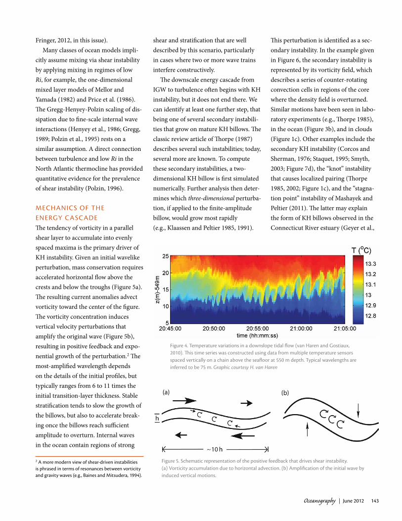
Figure 4. temperature variations in a downslope tidal flow (van Haren and Gostiaux, 2010). This time series was constructed using data from multiple temperature sensors spaced vertically on a chain above the seafloor at 550 m depth. typical wavelengths are inferred to be 75 m. Graphic courtesy H. van Haren

Figure 5. Schematic representation of the positive feedback that drives shear instability. (a) Vorticity accumulation due to horizontal advection. (b) amplification of the initial wave by induced vertical motions.

Oceanography | Vol. 25, No. 2144

2010) and on the Oregon continental shelf (Moum et al., 2003, shown in Figure 8). The question of which second-ary instabilities are most important for the development of turbulence in oce-anic billows remains unresolved. While complex, these secondary instabilities are not turbulent, so further transitions (i.e., tertiary instabilities and beyond) must be present. eVOlutION OF tHe INStaBIlIt y IN NuMerIcal SIMul atIONSWith recent increases in computational power, it has become feasible to study the energy cascade via direct simulation of the full three-dimensional dynam-ics. Through direct numerical simula-tions, we are uniquely able to examine in detail the full evolutionary cycle of flow instabilities. Simulations are limited by available computer memory and, therefore, cannot fully replicate the range of interactions that occur in geophysi-cal flows. However, with full resolution of the smallest scales, they reveal both the nonlinear evolution of the primary instability and the sequence of second-ary instabilities that leads to turbulence. Moreover, simulations furnish a quan-titative representation of the resulting turbulence and the mixing it causes.

The first numerical simulations of KH instability were restricted to two dimensions due to memory limitations (e.g., Patnaik et al., 1976; Klaassen and Peltier, 1985). These simulations con-firmed the primary instability but could not resolve the subsequent transition to three-dimensional motion. Three-dimensional simulations became pos-sible in the 1990s (Caulfield and Peltier, 1994; Scinocca, 1995) and have been used in numerous studies since then as

Figure 6. Secondary instability of a Kelvin-Helmholtz billow calculated using perturbation analysis. colors show the perturbation vorticity field. yellow indicates perturbations of the spanwise (y) vorticity that defines the primary instability. red and blue show opposite signs of the streamwise (x) vorticity.

Figure 7. Direct numerical simulations of the density field at successive time in the life cycle of a Kelvin-Helmholtz billow train. colors show density in the transition layer; upper and lower homo-geneous layers are rendered transparent. (a) The initial state is a two-layer flow, with a lower (dense) layer flowing to the left and an upper layer to the right. a small perturbation is applied. (b) two wavelengths of the primary Kelvin-Helmholtz instability. (c) Kelvin-Helmholtz billows are beginning to pair. Secondary instability is visible in a cutaway at upper right, taking the form of shear-aligned convection rolls. (d) Secondary shear instability forms on the braids. (e) The fully turbulent state. (f) turbulence decays to form sharp layers and random small-scale waves.

Oceanography | June 2012 145

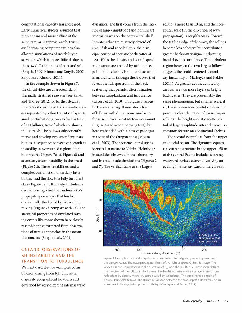
dynamics. The first comes from the inte-rior of large-amplitude (and nonlinear) internal waves on the continental shelf. In waters that are relatively devoid of small fish and zooplankton, the prin-cipal source of acoustic backscatter at 120 kHz is the density and sound speed microstructure created by turbulence, a point made clear by broadband acoustic measurements through these waves that reveal the full spectrum of the back-scattering that permits discrimination between zooplankton and turbulence (Lavery et al., 2010). In Figure 8, acous-tic backscattering illuminates a train of billows with dimensions similar to those seen over Great Meteor Seamount (Figure 4 and accompanying text), but here embedded within a wave propagat-ing toward the Oregon coast (Moum et al., 2003). The sequence of rollups is identical in nature to Kelvin–Helmholtz instabilities observed in the laboratory and in small-scale simulations (Figures 2 and 7). The vertical scale of the largest

rollup is more than 10 m, and the hori-zontal scale (in the direction of wave propagation) is roughly 50 m. Toward the trailing edge of the wave, the rollups become less coherent but contribute a greater backscatter signal, indicating breakdown to turbulence. The turbulent region between the two largest billows suggests the braid-centered second-ary instability of Mashayek and Peltier (2011). At greater depth, denoted by arrows, are two more layers of bright backscatter. They are presumably the same phenomenon, but smaller scale; if so, the echosounder resolution does not permit a clear depiction of these deeper rollups. The bright acoustic scattering tail of large-amplitude internal waves is a common feature on continental shelves.

The second example is from the upper equatorial ocean. The signature equato-rial current structure in the upper 150 m of the central Pacific includes a strong westward surface current overlying an equally intense eastward undercurrent.

Dep

th (m

)

20

40

Distance along ship track (m) –200 –100 0 100 200

Figure 8. example acoustical snapshot of a nonlinear internal gravity wave approaching the Oregon coast. The wave propagates from left to right at speed Cw in this image. The velocity in the upper layer is in the direction of Cw, and the resultant current shear defines the direction of the rollups in the billows. The bright acoustic scattering layers result from reflections by density microstructure caused by turbulence. The signal reveals a train of Kelvin-Helmholtz billows. The structure located between the two largest billows may be an example of the stagnation point instability (Mashayek and peltier, 2011).

computational capacity has increased. Early numerical studies assumed that momentum and mass diffuse at the same rate, as is approximately true in air. Increasing computer size has also allowed simulations of instability in seawater, which is more difficult due to the slow diffusion rates of heat and salt (Smyth, 1999; Kimura and Smyth, 2007; Smyth and Kimura, 2011).

In the example shown in Figure 7, the diffusivities are characteristic of thermally stratified seawater (see Smyth and Thorpe, 2012, for further details). Figure 7a shows the initial state—two lay-ers separated by a thin transition layer. A small perturbation grows to form a train of KH billows, two of which are shown in Figure 7b. The billows subsequently merge and develop two secondary insta-bilities in sequence: convective secondary instability in overturned regions of the billow cores (Figure 7c, cf. Figure 6) and secondary shear instability in the braids (Figure 7d). These instabilities, and a complex combination of tertiary insta-bilities, lead the flow to a fully turbulent state (Figure 7e). Ultimately, turbulence decays, leaving a field of random IGWs propagating on a layer that has been dramatically thickened by irreversible mixing (Figure 7f, compare with 7a). The statistical properties of simulated mix-ing events like those shown here closely resemble those extracted from observa-tions of turbulent patches in the ocean thermocline (Smyth et al., 2001).

OceaNIc OBSerVatIONS OF KH INStaBIlIt y aND tHe tr aNSItION tO turBuleNceWe next describe two examples of tur-bulence arising from KH billows in disparate geographical locations and governed by very different internal wave

Oceanography | Vol. 25, No. 2146

now used routinely in data analysis. Linear stability analysis provides com-pelling evidence that the oscillations found in strongly sheared equatorial currents are, in fact, a KH instability. Predicted wavelengths of computed instabilities (Sun et al., 1998; Figure 10a) agree with directly measured wave-lengths (Moum et al., 1992), and pre-dicted frequencies (Smyth et al., 2011; Figure 10b) also agree well with directly measured frequencies (Moum et al., 2011). These analyses show that the con-ditions for the growth of KH instability occur sporadically, which in turn sug-gests that random internal wave interac-tions add to the ambient shear to drive Ri to subcritical values, thereby generat-ing instability at random points in space and time. The similarity between the dominant frequency of the oscillations and N is consistent with this scenario, even though the frequency of individual KH events is independent of stratifica-tion (see Box 1).

The relationship between KH instabil-ity and small-scale turbulence is com-plex: the instability causes turbulence, and turbulence already present in the environment affects its growth. Liu et al. (2011) have recently extended the classi-cal method of stability analysis to include the effects of ambient turbulence. In strongly forced flows, such as exist in the upper equatorial ocean, this relationship can lead to a cycle in which shear is con-tinually reinforced, but new instabilities cannot grow until turbulence generated by previous instabilities decays.

As a result, current shear is large and, despite strong stratification, Ri is typi-cally near-critical in the mean.3 It has long been suspected that turbulence generated beneath the equatorial mixed layer (which does not generally extend as far as it does beneath mid-latitude mixed layers) is due to shear instabil-ity. Recent measurements from a verti-cal array of fast temperature sensors moored for extended periods in the upper equatorial ocean have confirmed the basic structure of KH instability in the small-scale fluctuations that appear on a daily cycle at frequencies near the local buoyancy frequency, N (Figure 9; Moum et al., 2011). The frequency and intermittency of the fluctuations can be seen in the Figure 9a spectrogram. The

phase of the oscillations varies vertically in a manner consistent with KH instabil-ity. Oscillations typically comprise O(10) wavelengths. Potential energy stored in these motions (Figure 9b) also varies on a daily basis and is correlated with the turbulent kinetic energy dissipation rate (Figure 9c), indicating that turbulent mixing at small scales coincides with KH billows (Figure 9d).

The interpretation of these fluctua-tions as KH billows has been tested via application to oceanic data of Rayleigh’s (1880) method of linear stability analy-sis. That method has been used in the interpretation of billows observed in the atmosphere (Busack and Brummer, 1988) and in the ocean (Mack and Hebert, 1997; Sun et al., 1998), and is

3 In the case of large-amplitude internal waves, the shear at a point in space is short-lived, and so also is near-critical Ri. The important issue of how long near-critical Ri must persist for instability to occur has been examined in laboratory and numerical experiments (Fructus et al., 2009; Inoue and Smyth, 2009; Barad and Fringer, 2010).

Figure 9. tempera-ture fluctuations observed in the sheared zone above the pacific equato-rial undercurrent. (a) temperature spectrogram (vari-ance preserving), (b) wave potential energy, NT

2 ζ 2, and (c) turbulence

f • Φ

T (K2 )

0.00

0.02

log 10

freq

uenc

y (H

z)N

T2ζ2 (m

2 s–2

)

–3

–4

10–6

10–10

ε χ (m

2 s–3

)

10–6

10–8

a

b

c

d

January 1, 2007 February 1, 2007

29 m

log 10

ε χ (m

2 s–3

)

log10NT2ζ2 (m2 s–2)

–4

–6

–8

τ ~ 102 s

τ ~ 103 s

τ ~ 104 s

–6 –4 –2

f • Φ

T (K2 )

0.00

0.02

log 10

freq

uenc

y (H

z)N

T2ζ2 (m

2 s–2

)

–3

–4

10–6

10–10

ε χ (m

2 s–3

)

10–6

10–8

a

b

c

d

January 1, 2007 February 1, 2007

29 m

log 10

ε χ (m

2 s–3

)

log10NT2ζ2 (m2 s–2)

–4

–6

–8

τ ~ 102 s

τ ~ 103 s

τ ~ 104 s

–6 –4 –2

f • Φ

T (K2 )

0.00

0.02

log 10

freq

uenc

y (H

z)N

T2ζ2 (m

2 s–2

)

–3

–4

10–6

10–10

ε χ (m

2 s–3

)

10–6

10–8

a

b

c

d

January 1, 2007 February 1, 2007

29 m

log 10

ε χ (m

2 s–3

)

log10NT2ζ2 (m2 s–2)

–4

–6

–8

τ ~ 102 s

τ ~ 103 s

τ ~ 104 s

–6 –4 –2

dissipation rate, εχ , for the period December 20, 2006–February 10, 2007, derived from a single fast thermistor deployed at 29 m on NOaa’s taO (tropical Ocean-atmosphere) mooring at 0°, 140°W. The relationship between the potential energy of the instabilities and the turbulence is established in the scatter plot (d). Blue points plotted represent the two-dimensional histogram; darker points occur more frequently.

Oceanography | June 2012 147

b

a0.12

0.10

0.08

0.06

0.04

0.02

0.00

40

30

20

10

0

0.020

0.015

0.010

0.005

0.000

29 m39 m49 m59 m

Gro

wth

rate

(x 1

0–2s–1

)

# un

stab

le m

odes

–8 –6 –4 –2 0 2 4 6l (x 10 –2 rad/m) 0

2

2

1

4

4

6

k (x 10–2 rad/m)

f • Φ

T (K2 )

log10|f| (Hz) –4.0 –3.8 –3.6 –3.4 –3.2 –3.0 –2.8 –2.6 –2.4 –2.2 –2.0

Figure 10. linear stability analyses of flow above the pacific equatorial undercurrent. (a) Growth rate versus zonal and meridional wavenumbers. colors represent mode families focused in different shear layers between the undercurrent core and the surface (Sun et al., 1998). Graphic cour-tesy C. Sun. (b) Histogram of absolute cyclic frequency for 155 unstable modes computed numerically from hourly averaged profiles of velocity and density (Smyth et al., 2011). curves show normalized, variance-preserving spectra of four observed temperature time series. Sensor depths are as shown in the legend.

BOx 1 | WHy KelVIN-HelMHOltz BIllOWS are Near-N

Umin Umax

Pc

c0 λ0

λ

Pλ

log10 | f | (Hz)

P log 10

|f|

–4.0 –3.5 –3.0 –2.5 –2.0

1.6

1.4

1.2

1.0

0.8

0.6

0.4

0.2

0.0

Figure B3. probability distribution function for the frequency: theoretical (blue) and based on linear stability analysis of mea-sured flows (gray).

Figure B1. probability distri-bution of phase velocity.

Figure B2. probability dis-tribution of wavelength.

Oscillations in the upper equatorial pacific, thought to arise from KH instability, show a striking tendency to have frequency close to N, the buoyancy frequency. This is not a property of individual KH billows, but may follow from the statistics of a random ensemble of instabilities due to sporadic shear amplification by interacting gravity waves.

consider a random ensemble of instabilities growing on small shear layers within a larger sheared zone. phase velocities lie approximately within the range of the mean current (Howard, 1961; Figure B1), Umin < c < Umax. The observer’s velocity is assumed to lie in the range of the mean flow, so that Umin < 0 and Umax > 0. Wavelengths lie between zero and about seven times the thickness of the largest shear layer (e.g., Hazel, 1972; Figure B2).

treating phase velocity and wavelength as independent random variables yields a probability distribution function for the frequency (Figure B3), shown in blue for representative values Umin = –1 ms–1, Umax = 1 ms–1, and λ0 = 700 m. For comparison, gray bars show the frequency distribution of instabilities computed via linear stability analysis of the observed velocity and density profiles. The theo-retical peak frequency, fpeak = max (|Umin|, Umax)/λ0, is consistent with that of computed instabilities for this regime, and also with observations (Figure 10).

Given that the maximum possible wavelength λ0 is about 2π times the thickness D of the sheared zone, the peak angular frequency ωpeak = 2π fpeak is within a factor two of the mean shear. (Since Umin < 0, the mean shear would be (Umax + |Umin |)/D, and the sum of two posi-tive numbers is, at most, twice the greater.) The mean flow is character-ized by richardson number of order unity, hence N and the shear are nearly equal, implying that ωpeak ~ N.

Oceanography | Vol. 25, No. 2148

QuaNtIF yING MIxING By KH INStaBIlIt yTo determine the net contribution of KH instability to global mixing, two critical challenges must be addressed. The first is to quantify the prevalence of KH instability in thermocline internal wave fields. Other forms of instabil-ity contribute to thermocline mixing. How much? One way this quantity is being measured is with long time series that include sufficient detail to diagnose KH instability in the sig-nal such as those made in the upper equatorial ocean by Moum et al. (2011; Figure 9). Can thermocline observations with the same fidelity be obtained that permit an evaluation of the prevalence of KH instability in thermocline internal wave fields? Glider measurements are promising in this respect (e.g., Thorpe 2012; Smyth and Thorpe 2012.)

The second challenge is to param-eterize KH-induced mixing (i.e., to approximate the rate of mixing in terms of other quantities that are more easily measured or modeled). For example, Kunze et al. (1990) used a simple analyti-cal model of a shear layer to estimate the mean flow kinetic energy released in an instability event and combined the result with an estimate of the turbulence production time to arrive at the kinetic energy dissipation rate. Future param-eterizations will incorporate more com-plete models of instability physics, and they will be calibrated using advanced laboratory techniques, comprehensive microstructure observations, and direct numerical simulations of increasing scale and realism.

acKNOWleDGeMeNtSOur work on KH instability has been funded by the National Science Foundation (1030772 and 1129419 to WDS, and 0728357 and 1059055 to JNM) and by the Office of Naval Research (N00014-09-1-0280, N000014-10-1-2098 to JNM). Helpful critiques of this article were provided by Steve Thorpe, Aurelie Moulin, Elizabeth McHugh and two anonymous referees.

reFereNceSBaines, P.G., and H. Mitsudera. 1994. On the

mechanism of shear flow instabilities. Journal of Fluid Mechanics 276:327–342, http://dx.doi.org/ 10.1017/S0022112094002582.

Barad, M.F., and O.B. Fringer. 2010. Simulations of shear instabilities in interfacial gravity waves. Journal of Fluid Mechanics 644:61–95, http://dx.doi.org/10.1017/S0022112009992035.

Busack, B., and B. Brummer. 1988. A case study of Kelvin-Helmholtz waves within an off-shore stable boundary layer: Observations and linear model. Boundary-Layer Meteorology 44:105–135, http://dx.doi.org/ 10.1007/BF00117295.

Caulfield, C.P., and W.R. Peltier. 1994. Three-dimensionalization of the stratified mixing layer. Physics of Fluids A 6(12):3,803–3,805, http://dx.doi.org/10.1063/1.868370.

Corcos, G., and F. Sherman. 1976. Vorticity concentration and the dynamics of unstable free shear layers. Journal of Fluid Mechanics 73: 241–264, http://dx.doi.org/ 10.1017/S0022112076001365.

Dunkerton, T. 1997. Shear instability of internal inertia-gravity waves. Journal of the Atmospheric Sciences 54:1,628–1,641, http://dx.doi.org/ 10.1175/1520-0469(1997)054<1628:SIOIIG> 2.0.CO;2.

Fructus, D., M. Carr, J. Grue, A. Jensen, and P.A. Davies. 2009. Shear-induced breaking of large internal solitary waves. Journal of Fluid Mechanics 620:1–29, http://dx.doi.org/10.1017/S0022112008004898.

Geyer, W.R., A. Lavery, M.E. Scully, and J.H. Trowbridge. 2010. Mixing by shear insta-bility at high Reynolds number. Geophysical Research Letters 37, L22607, http://dx.doi.org/ 10.1029/2010GL045272.

Geyer, W.R., and J.D. Smith. 1987. Shear insta-bility in a highly stratified estuary. Journal of Physical Oceanography 17:1,668–1,679, http://dx.doi.org/10.1175/1520-0485(1987) 017<1668:SIIAHS>2.0.CO;2.

Goldstein, S. 1931. On the stability of super-posed streams of fluids of different densi-ties. Proceedings of the Royal Society of London A 132:524–548, http://dx.doi.org/ 10.1098/rspa.1931.0116.

Gregg, M.C. 1989. Scaling turbulent dissipation in the thermocline. Journal of Geophysical Research 94:9,686–9,698, http://dx.doi.org/ 10.1029/JC094iC07p09686.

Hazel, P. 1972. Numerical studies of the stability of inviscid stratified shear flows. Journal of Fluid Mechanics 51:39–61, http://dx.doi.org/10.1017/S0022112072001065.

Henyey, F.S., J. Wright, and S.M. Flatté. 1986. Energy and action flow through the internal wave field: An eikonal approach. Journal of Geophysical Research 91(C7):8,487–8,495, http://dx.doi.org/10.1029/JC091iC07p08487.

Hibiya, T., Y. Niwa, and K. Fujiwara. 1998. Numerical experiments of nonlinear energy transfer within the oceanic inter-nal wave spectrum. Journal of Geophysical Research 103(C9):18,715–18,722, http://dx.doi.org/10.1029/98JC01362.

Howard, L.N. 1961. Note on a paper of John W. Miles. Journal of Fluid Mechanics 10:509–512, http://dx.doi.org/10.1017/S0022112061000317.

Inoue, R., and W.D. Smyth. 2009. Efficiency of mixing forced by unsteady shear flow. Journal of Physical Oceanography 39:1,150–1,166, http://dx.doi.org/10.1175/2008JPO3927.1.

Kimura, S., and W.D. Smyth. 2007. Direct numeri-cal simulation of salt sheets and turbulence in a double-diffusive shear layer. Geophysical Research Letters 34, L21610, http://dx.doi.org/ 10.1029/2007GL031935.

Klaassen, G.P., and W.R. Peltier. 1985. The evolu-tion of finite-amplitude Kelvin-Helmholtz billows in two spatial dimensions. Journal of the Atmospheric Sciences 42:1,321–1,339, http://dx.doi.org/10.1175/1520-0469(1985) 042<1321:EOFAKB>2.0.CO;2.

Klaassen, G.P., and W.R. Peltier. 1991. The influ-ence of stratification on secondary insta-bility in free shear layers. Journal of Fluid Mechanics 227:71–106, http://dx.doi.org/ 10.1017/S0022112091000046.

Kunze, E., A.J. Williams III, and M.G. Briscoe. 1990. Observations of shear and vertical stabil-ity from a neutrally buoyant float. Journal of Geophysical Research 95:18,127–18,142, http://dx.doi.org/10.1029/JC095iC10p18127.

Lamb, K.G., and D. Farmer. 2011. Instabilities in an internal solitary-like wave on the Oregon shelf. Journal of Physical Oceanography 41:67–87, http://dx.doi.org/10.1175/2010JPO4308.1.

Lavery, A.C., D. Chu, and J.N. Moum. 2010. Observations of broadband acoustic backscat-tering from nonlinear internal waves: Assessing the contribution from microstructure. IEEE Journal of Ocean Engineering 35:695–709, http://dx.doi.org/10.1109/JOE.2010.2047814.

Lelong, M.-P., and T.J. Dunkerton. 1998a. Inertia-gravity wave breaking in three dimensions. Part I: Convectively stable waves. Journal

Oceanography | June 2012 149

of the Atmospheric Sciences 55:2,473–2,488, http://dx.doi.org/10.1175/1520-0469(1998) 055<2473:IGWBIT>2.0.CO;2.

Lelong, M.-P., and T.J. Dunkerton. 1998b. Inertia-gravity wave breaking in three dimensions. Part II: Convectively unsta-ble waves. Journal of the Atmospheric Sciences 55:2,489-2,501, http://dx.doi.org/ 10.1175/1520-0469(1998)055<2489:IGWBIT>2.0.CO;2.

Liu, Z., S.A. Thorpe, and W.D. Smyth. 2011. Instability and hydraulics of turbulent stratified shear flows. Journal of Fluid Mechanics 695:235–256, http://dx.doi.org/ 10.1017/jfm.2012.13.

Mack, A., and D. Hebert. 1997. Internal gravity waves in the upper eastern equatorial Pacific: Observations and numerical solutions. Journal of Geophysical Research 102:21,081–21,100, http://dx.doi.org/10.1029/97JC01506.

Mashayek, A., and W.R. Peltier. 2011. Three-dimensionalization of the stratified mixing layer at high Reynolds number. Physics of Fluids 23, 111701, http://dx.doi.org/10.1063/1.3651269.

Mellor, G., and T. Yamada. 1982. Development of a turbulence closure model for geophysical appli-cations. Reviews of Geophysics 20(4):851–875, http://dx.doi.org/10.1029/RG020i004p00851.

Miles, J.W. 1961. On the stability of hetero-geneous shear flows. Journal of Fluid Mechanics 10:496–508, http://dx.doi.org/ 10.1017/S0022112061000305.

Moum, J.N., D.M. Farmer, W.D. Smyth, L. Armi, and S. Vagle. 2003. Structure and gen-eration of turbulence at interfaces strained by internal solitary waves propagating shoreward over the continental shelf. Journal of Physical Oceanography 33:2,093–2,122, http://dx.doi.org/10.1175/1520-0485(2003) 033<2093:SAGOTA>2.0.CO;2.

Moum, J.N., D. Hebert, C.A. Paulson, and D.R. Caldwell. 1992. Turbulence and inter-nal waves at the equator. Part 1: Statistics from towed thermistors and a micro-structure profiler. Journal of Physical Oceanography 22:1,330–1,345, http://dx.doi.org/10.1175/1520-0485(1992)022 <1330:TAIWAT>2.0.CO;2.

Moum, J.N., J.D. Nash, and W.D. Smyth. 2011. Narrowband oscillations in the upper equatorial ocean. Part I: Interpretation as shear instabilities. Journal of Physical Oceanography 41:397–411, http://dx.doi.org/ 10.1175/2010JPO4450.1.

Patnaik, P., F.S. Sherman, and G.M. Corcos. 1976. A numerical simulation of Kelvin-Helmholtz waves of finite amplitude. Journal of Fluid Mechanics 73:215–240, http://dx.doi.org/ 10.1017/S0022112076001353.

Polzin, K.L. 1996. Statistics of the Richardson num-ber: Mixing models and finestructure. Journal of Physical Oceanography 26:1,409–1,425, http://dx.doi.org/10.1175/1520-0485(1996)026 <1409:SOTRNM>2.0.CO;2.

Polzin, K.L., J.M. Toole, and R.W. Schmitt. 1995. Finescale parameterizations of tur-bulent dissipation. Journal of Physical Oceanography 25:306–328, http://dx.doi.org/ 10.1175/1520-0485(1995)025<0306:FPOTD>2.0.CO;2.

Price, J.F., R.A. Weller, and R. Pinkel. 1986. Diurnal cycling: Observations and models of the upper ocean response to diurnal heating, cool-ing and wind mixing. Journal of Geophysical Research 91(C7):8,411–8,427, http://dx.doi.org/ 10.1029/JC091iC07p08411.

Rayleigh, L. 1880. On the stability or instability of certain fluid motions. Proceedings of the London Mathematical Society 11:57–70, http://dx.doi.org/10.1112/plms/s1-11.1.57.

Reynolds, O. 1883. An experimental investigation of the circumstances which determine whether the motion of water shall be direct or sinuous, and of the law of resistance in parallel chan-nels. Philosophical Transactions of the Royal Society 174:935–982.

Scinocca, J.F. 1995. The mixing of mass and momentum by Kelvin-Helmholtz billows. Journal of the Atmospheric Sciences 52:2,509–2,530.

Smyth, W.D. 1999. Dissipation range geometry and scalar mixing in sheared, stratified turbulence. Journal of Fluid Mechanics 401:209–242.

Smyth, W.D. 2003. Secondary Kelvin-Helmholtz instability in weakly stratified shear flow. Journal of Fluid Mechanics 497:67–98, http://dx.doi.org/10.1017/S0022112003006591.

Smyth, W.D., and S. Kimura. 2011. Mixing in a moderately sheared salt fingering layer. Journal of Physical Oceanography 41:1,361–1,381, http://dx.doi.org/10.1175/2010JPO4611.1.

Smyth, W.D., J.N. Moum, and D.R. Caldwell. 2001. The efficiency of mixing in turbulent patches: Inferences from direct simulations and microstructure observations. Journal of Physical Oceanography 31:1,969–1,992, http://dx.doi.org/10.1175/1520-0485(2001)031 <1969:TEOMIT>2.0.CO;2.

Smyth, W.D., J.N. Moum, and J.D. Nash. 2011. Narrowband oscillations in the upper equatorial ocean. Part II: Properties of shear instabilities. Journal of Physical Oceanography 41:412–428, http://dx.doi.org/10.1175/2010JPO4451.1.

Smyth, W.D., and S.A. Thorpe. 2012. Glider measurements of overturning in a Kelvin-Helmholtz billow train. Journal of Marine Research 70:117–140.

Staquet, C. 1995. Two-dimensional secondary instabilities in a strongly stratified shear layer. Journal of Fluid Mechanics 296:73–126, http://dx.doi.org/10.1017/S0022112095002072.

Stern, M.E. 1969. Collective instability of salt fin-gers. Journal of Fluid Mechanics 35:209–218, http://dx.doi.org/10.1017/S0022112069001066.

Sun, C., W.D. Smyth, and J.N. Moum. 1998. Dynamic instability of stratified shear flow in the upper equatorial Pacific. Journal of Geophysical Research 103(C5):10,323–10,337, http://dx.doi.org/10.1029/98JC00191.

Taylor, G.I. 1927. An experiment on the stability of superposed streams of fluid. Proceedings of the Cambridge Philosophical Society 23:730–731, http://dx.doi.org/10.1017/S0305004100011245.

Taylor, G.I. 1931. Effect of variation in den-sity on the stability of superposed streams of fluid. Proceedings of the Royal Society of London 132:499–523, http://dx.doi.org/10.1098/rspa.1931.0115.

Thomson, W. (Lord Kelvin). 1871. Hydrokinetic solutions and observations. Philosophical Magazine 42:362–377.

Thorpe, S.A. 1969. Neutral eigensolutions of the stability equation for stratified shear flow. Journal of Fluid Mechanics 36:673–683, http://dx.doi.org/10.1017/S0022112069001923.

Thorpe, S.A. 1971. Experiments on the instabil-ity of stratified shear flows: Miscible fluids. Journal of Fluid Mechanics 46:299–319, http://dx.doi.org/10.1017/S0022112071000557.

Thorpe, S.A. 1985. Laboratory observations of secondary structures in Kelvin-Helmholtz billows and consequences for ocean mix-ing. Geophysical and Astrophysical Fluid Dynamics 34:175–199.

Thorpe, S.A. 1987. Transition phenomena and the development of turbulence in stratified fluids. Journal of Geophysical Research 92(C5):5,231–5,245, http://dx.doi.org/10.1029/JC092iC05p05231.

Thorpe, S.A. 2002. The axial coherence of Kelvin–Helmholtz billows. Quarterly Journal of the Royal Meteorological Society 128:1,529–1,542, http://dx.doi.org/10.1002/qj.200212858307.

Thorpe, S.A. 2012. Measuring overturns with glid-ers. Journal of Marine Research 70:93–117.

van Haren, H., and L. Gostiaux. 2010. A deep-ocean Kelvin‐Helmholtz billow train. Geophysical Research Letters 37, L03605, http://dx.doi.org/10.1029/2009GL041890.

Venayagamoorthy, S.K., and O.B. Fringer. 2012. Examining breaking internal waves on a shelf slope using numerical simula-tions. Oceanography 25(2):132–139, http://dx.doi.org/10.5670/oceanog.2012.48.

von Helmholtz, H. 1890. Die energie der wogen und des windes. Annalen der Physik 41:641–662, http://dx.doi.org/10.1002/andp.18902771202.

Wesson, J.C., and M.C. Gregg 1994. Mixing at Camarinal Sill in the Strait of Gibraltar. Journal of Geophysical Research 99(C5):9,847–9,878, http://dx.doi.org/10.1029/94JC00256.

Woods, J.D. 1968. Wave-induced shear instabil-ity in the summer thermocline. Journal of Fluid Mechanics 32:791–800, http://dx.doi.org/ 10.1017/S0022112068001035.