Odd-Parity Bipolar Spherical Harmonics

Laura G. Book1, Marc Kamionkowski12, and Tarun Souradeep3

1California Institute of Technology, Mail Code 350-17, Pasadena, CA 911252Johns Hopkins University, Department of Physics and Astronomy,Bloomberg 439, 3400 N. Charles St., Baltimore, MD 21218 and

3Inter-University Centre for Astronomy and Astrophysics, Pune 411007, India(Dated: November 21, 2011)

Bipolar spherical harmonics (BiPoSHs) provide a general formalism for quantifying departuresin the cosmic microwave background (CMB) from statistical isotropy (SI) and from Gaussianity.However, prior work has focused only on BiPoSHs with even parity. Here we show that thereis another set of BiPoSHs with odd parity, and we explore their cosmological applications. Wedescribe systematic artifacts in a CMB map that could be sought by measurement of these odd-parity BiPoSH modes. These BiPoSH modes may also be produced cosmologically through lensingby gravitational waves (GWs), among other sources. We derive expressions for the BiPoSH modesinduced by the weak lensing of both scalar and tensor perturbations. We then investigate thepossibility of detecting parity-breaking physics, such as chiral GWs, by cross-correlating oppositeparity BiPoSH modes with multipole moments of the CMB polarization. We find that the expectedsignal-to-noise of such a detection is modest.

I. INTRODUCTION

The detection of anisotropies in the cosmic microwave background (CMB) [1] has revolutionized the precision withwhich cosmological measurements can be made. Most of the information that has been obtained from the CMB sofar has come from its power spectrum, the two-point correlation function, under the assumptions of isotropy andhomogeneity. However, in recent years, attention has been paid to effects that go beyond the power spectrum, such asweak lensing [2], cosmic birefringence [3, 4], and departures from statistical isotropy (SI) [5–7] and from Gaussianity[8–10].

Bipolar spherical harmonics (BiPoSHs) [11–13] provide an elegant and general formalism for quantifying a numberof these physical effects. If the CMB map is Gaussian and statistically isotropic, then its statistics are specifiedentirely in terms of the power spectrum Cl, the expectation value of the squared magnitude of the spherical-harmoniccoefficients alm for the map, and there are no correlations between different alms. A wide variety of departures fromSI and Gaussianity induce correlations between different alms. The point of the BiPoSH formalism is to parametrizecorrelations between two different coefficients, alm and al′m′ , that represent two different “angular-momentum” states,in terms of total angular momenta L and M . Bipolar spherical harmonics have been used to search for non-standardcosmic topology [14], anisotropy in primordial power [7, 15], and model-independent departures from SI [13, 16–21].They have also been used to test for asymmetric beams [22] and/or other systematic artifacts in WMAP [23]. BiPoSHsfor polarization have been proposed to search for position-dependent rotation of the CMB polarization [24–26].

However, there is still more that can be done with bipolar spherical harmonics, and the purpose of this paper is toenumerate some of them. First and foremost, we point out here that almost all prior work on BiPoSHs has consideredonly BiPoSHs with even parity (Sec. II). There exists an entire other set of BiPoSHs that have the opposite parity,and these can provide probes of both cosmological effects and systematic artifacts that would remain elusive with theeven-parity BiPoSHs that have been considered so far. We show, for example, that lensing by gravitational waves(GWs) can excite odd-parity BiPoSHs, and we describe a pointing error that could also excite these modes. In theprocess, we also show how gravitational lensing, by both density perturbations as well as GWs, can be described interms of even- and odd-parity BiPoSHs (Sec. III). Finally, we discuss how odd-parity BiPoSHs could be used as probesof parity violation, and consider in particular the cross-correlation of opposite parity CMB lensing and polarizationcomponents (Sec. IV). We calculate the anticipated spectra and errors for such correlations, and determine that alarge signal-to-noise is not expected for these cross-correlations, given the current upper bounds on a GW background.

arX

iv:1

109.

2910

v2 [

astr

o-ph

.CO

] 1

8 N

ov 2

011

2

II. REVIEW OF BIPOLAR SPHERICAL HARMONICS

A. Statistically Isotropic and Gaussian Maps

A CMB temperature map T (n), as a function of position n on the sky, can be decomposed into spherical-harmoniccoefficients

alm =

∫d2n T (n)Y ∗lm(n).

If the map is statistically isotropic and Gaussian, then the statistics can be determined entirely in terms of the powerspectrum Cl, defined by

〈alma∗l′m′〉 = Cl δll′ δmm′ , (1)

where the angle brackets denote an average over all realizations, and δll′ and δmm′ are Kronecker deltas. Eq. (1)states that all of the alm are uncorrelated, and Gaussianity further dictates that the probability distribution functionfor any alm to take on a particular value is a Gaussian distribution with variance Cl.

The spatial temperature autocorrelation function is defined to be C(n, n′) ≡ 〈T (n)T (n′)〉. Most generally it is afunction of the two directions n and n′. However, if the map is statistically isotropic and Gaussian, then the spatialcorrelation function depends only on the angle θ, given by cos θ = n · n′, between the two directions. In this case,

C(n, n′) =∑l

(2l + 1)

4πClPl(n · n′),

where Pl(x) are the Legendre polynomials.

B. Departures from Gaussianity/SI

Departures from Gaussianity and/or SI will induce correlations between different alms. The most general correlationbetween any two alms can be written,

〈alma∗l′m′〉 = Clδll′δmm′ +∑

LM ;L>0

(−1)m′〈l m l′, −m′|LM〉ALMll′ , (2)

where Cl is the (isotropic) power spectrum, 〈l m l′m′|LM〉 are Clebsch-Gordan coefficients, and the ALMll′ are BiPoSHcoefficients. The spatial two-point correlation function is then

C(n, n′) =∑l

(2l + 1)

4πClPl(n · n′) +

∑ll′LM

ALMll′ Yl(n)⊗ Yl′(n′)LM , (3)

where

Yl(n)⊗ Yl′(n′)LM =∑mm′

〈l m l′m′|LM〉Ylm(n)Yl′m′(n′), (4)

are the bipolar spherical harmonics (BipoSHs). These BiPoSHs constitute a complete orthonormal basis for functionsof n and n′ in terms of total-angular-momentum states labeled by quantum numbers L and M composed of angular-momentum states with lm and l′m′; they are an alternative to the outer product of the l,m and l′,m′ bases.

C. Odd-Parity Bipolar Spherical Harmonics

It is instructive to decompose ALMll′ into its odd and even parity parts,

ALMll′ = A⊕LMll′

[1 + (−1)l+l′+L]

2+A

LMll′

[1− (−1)l+l′+L]

2, (5)

3

where A⊕LMll′ (A

LMll′ ) are zero for the sum l + l′ + L being odd (even). It follows from the symmetry C(n, n′) =

C(n′, n) that A⊕LMll′ (A

LMll′ ) are (anti) symmetric in l and l′. We also infer that

[A⊕

LMll′

]∗= (−1)MA⊕

L−Mll′ and[

ALMll′

]∗= (−1)M+1A

L−Mll′ . Thus, odd-parity BiPoSHs vanish for l = l′. Prior literature has considered physical

effects (e.g., nontrivial topologies [27], SI violation [13, 28]) that produce only A⊕LMll′ , the even-parity BiPoSHs, and

measurements have been carried out with WMAP data only for the A⊕LMll′ [16, 29]. In this paper, we consider also

the odd-parity BiPoSHs ALMll′ .

Estimators for the BiPoSH coefficients (both the ⊕ and modes) can be constructed from a map of the CMBtemperature field T (n), as follows:

ALMll′ =∑mm′

W−1l W−1

l′ amaplm a∗map

l′m′ (−1)m′〈l m l′, −m′|LM〉, (6)

and this estimator has a variance, under the null hypothesis (a SI Gaussian map),⟨ALMll′ AL

′M ′

ll′

∗⟩= δLL′ δMM ′

[δllδl′ l′ + (−1)l+l

′+Lδll′δll′]Cmapl Cmap

l′ W−2l W−2

l′ , (7)

where amaplm = Wl alm + anoise

lm and Cmapl = W 2

l Cl + Nl are the temperature spherical-harmonic coefficients andpower spectrum corrected for detector noise and finite resolution. The Gaussian detector window function, whichencapsulates the effects of finite detector resolution, is given by Wl ≡ exp

[−l2θ2

FWHM/(16 ln 2)], where θFWHM is the

full width at half maximum of the detector. The instrumental noise contribution to the temperature power spectrumis given by

Nl =4π(NET)2

tobs

√fsky

,

where fsky is the fraction of the sky observed, NET is the noise equivalent temperature of the detector, and tobs isthe length of time over which the CMB was observed by a particular survey. We notice that the variance in Eq. (7)vanishes for odd parity and l = l′ = l = l′, which is expected given that odd-parity BiPoSHs with l = l′ vanish.

The noise in any individual ALMll′ is large, and so a search for a statistically significant departure from zero in oneor a handful of ALMll′ s will probably not be too effective. It is better to consider specific models and/or parame-terizations for departures from SI/Gaussianity and then combine the ALMll′ s into a minimum-variance estimator forthe SI/Gaussianity-violating parameters of those models. For example, Ref. [11, 12] considered the bipolar powerspectrum κL ≡

∑ll′M |ALMll′ |2 as a parameterization for departures from SI. As another example, Ref. [15] combined

ALMll′ s with L = 2 and l′ = l, l ± 2 to derive minimum-variance estimators for the amplitude of an inflation-inducedprimordial-power quadrupole of the type considered in Ref. [30].

III. GRAVITATIONAL LENSING

A. Gradient and Curl-Type Deflections

Consider a statistically isotropic and homogeneous Gaussian temperature map Tg(n) on the sphere, where n is a

position on the sky. Now suppose that each point on the sky n has been deflected from an original direction n+ ~∆(n)

so that the observed temperature is T (n) = Tg(n + ~∆) ' Tg(n) + ~∆ · ~∇~θTg(n). This deflection might come aboutcosmologically through weak gravitational lensing or may arise as an instrumental/measurement artifact (for example,if there are pointing errors).

The most general deflection field ~∆ can be written in vector notation as

~∆ = ~∇~θ φ(n) + ~∇~θ × Ω(n), (8)

or in component notation, ∆i =(∇~θ)iφ(n) + εij

(∇~θ)j

Ω(n),1 in terms of two scalar functions φ(n) and Ω(n) on the

sphere, where ~∇~θ is the angular covariant derivative on the unit sphere. In other words, the most general vector field

1 Here, the Levi-Civita symbol on the unit sphere can be defined in terms of its three-dimensional equivalent as εij = −εijk rk. Thechoice of sign here can be understood as the choice to have the spherical polar coordinates (θ, φ) form a right-handed coordinate systemon the sky, since it will ensure that the basis vectors satisfy eθ × eφ = 1.

4

on a two-sphere can be written as the gradient of some scalar field φ(n) plus the curl of some other field Ω(n). Weakgravitational lensing by density perturbations gives rise, at linear order in the lensing potential, only to the gradientcomponent. A curl component can arise cosmologically from second-order terms in the deflection field or from lensingby GWs. Systematic measurement effects may conceivably give rise to both types of deflections.

We now show that the A⊕LMll′ and A

LMll′ BiPoSH coefficients are induced, respectively, by the gradient and curl

components of the deflection field. The change in the temperature moments induced by lensing is (at first order in φand Ω),

δalm =

∫d2n Y ∗lm(n)

[~∇~θ φ

]·[~∇~θ T (n)

]+[~∇~θ Ω(n)

]×[~∇~θ T (n)

]=

∑LM ;L>0

∑l′m′

al′m′

∫d2n Y ∗lm(n)

φLM

[~∇~θ YLM (n)

]·[~∇~θ Yl′m′(n)

]+ ΩLM

[~∇~θ YLM (n)

]×[~∇~θ Yl′m′(n)

],

where in the second line we have decomposed

φ(n) =

∞∑L=1

L∑M=−L

YLM (n) φLM , (9)

and similarly for Ω(n). We do not consider L = 0 modes of φ and Ω since they would not cause a deflection. In thenotation of Ref. [31],

~∇~θ Ylm =

√l(l + 1)

2[1Ylm m+ − −1Ylm m−] ,

where 1Ylm and −1Ylm are spin-weighted spherical harmonics, the null coordinates m± = (eθ∓ ieφ)/√

2, and the onlynon-trivial products of the null coordinates are m+ · m− = 1, and m+ × m− = i. Thus, it is obtained that(

~∇~θ YLM)·(~∇~θ Yl′m′

)= −

√L(L+ 1)l′(l′ + 1)

2[(1YLM ) (−1Yl′m′) + (−1YLM ) (1Yl′m′)] ,(

~∇~θ YLM)×(~∇~θ Yl′m′

)= −

i√L(L+ 1)l′(l′ + 1)

2[(1YLM ) (−1Yl′m′)− (−1YLM ) (1Yl′m′)] .

Using the triple integral [31] of spin-weighted spherical harmonics, the δalm for the gradient and curl terms areobtained as

δalm =∑

LM ;L>0

∑l′m′

(−1)M+m al′m′ GLll′√(2L+ 1)l(l + 1)

φLM[1 + (−1)l+l

′+L]

2− iΩLM

[1− (−1)l+l

′+L]

2

〈l m l′, −m′|LM〉,

where

GLll′ ≡√L(L+ 1)l(l + 1)l′(l′ + 1)(2l + 1)(2l′ + 1)

4π〈l 0 l′ 1|L1〉.

Up to linear order in the deflection coefficients φLM and ΩLM , the even- and odd-parity BiPoSH coefficients are then,

A⊕LMll′ =

φLM√2L+ 1

[ClG

Ll′l√

l′(l′ + 1)+

Cl′GLll′√

l(l + 1)

]= Q⊕Lll′ φLM , (10)

ALMll′ =

iΩLM√2L+ 1

[ClG

Ll′l√

l′(l′ + 1)− Cl′G

Lll′√

l(l + 1)

]= QLll′ ΩLM , (11)

where we have defined the quantities

Q⊕Lll′ =1√

2L+ 1

[ClG

Ll′l√

l′(l′ + 1)+

Cl′GLll′√

l(l + 1)

],

QLll′ =i√

2L+ 1

[ClG

Ll′l√

l′(l′ + 1)− Cl′G

Lll′√

l(l + 1)

].

5

Clearly, the gradient part contributes only to A⊕LMll′ and the curl part only to A

LMll′ . Further, it is explicit that the

gradient and curl parts of the deflection correspond, respectively, to the symmetric and antisymmetric (in ll′) partsof the total ALMll′ .

Suppose the ALMll′ s have been measured using the estimators in Eq. (6). If we then assume that lensing is thedominant source of BiPoSHs we can use Eqs. (7), (10), and (11) to construct maximum-likelihood estimators for thegradient and curl components of the deflection field,

φLM =

∑ll′ Q

⊕L∗ll′ A⊕LMll′

/ (W−2l W−2

l′ Cmapl Cmap

l′

)∑ll′

∣∣Q⊕Lll′ ∣∣2 / (W−2l W−2

l′ Cmapl Cmap

l′

) , (12)

ΩLM =

∑ll′ Q

L∗ll′ ALMll′

/ (W−2l W−2

l′ Cmapl Cmap

l′

)∑ll′

∣∣QLll′ ∣∣2 / (W−2l W−2

l′ Cmapl Cmap

l′

) . (13)

The variance of these estimators, under the null hypothesis of no lensing, is given by

〈φLM φL′M ′∗〉 ≡ δLL′ δMM ′

(σφL)2 ≡ 2 δLL′ δMM ′

[∑ll′

∣∣Q⊕Lll′ ∣∣2 / (W−2l W−2

l′ Cmapl Cmap

l′

)]−1

, (14)

〈ΩLM ΩL′M ′∗〉 ≡ δLL′ δMM ′

(σΩL

)2 ≡ 2 δLL′ δMM ′

[∑ll′

∣∣QLll′ ∣∣2 / (W−2l W−2

l′ Cmapl Cmap

l′

)]−1

, (15)

where the sums in Eqs. (12) and (14) only include pairs of l, l′ for which l + l′ + L is even, while those in Eqs. (13)and (15) only include pairs for which this quantity is odd.

B. Deflection Field from Metric Perturbations

Cosmic shear, weak gravitational lensing due to density perturbations or GWs along the line of sight to the CMB,will produce displacements like those in Eq. (8). Our goal here will be to calculate the displacement spherical-harmoniccoefficients φLM and ΩLM that arise from gravitational lensing due to density perturbations and GWs. There is a vastliterature on lensing by density perturbations and also specifically on lensing of the CMB by density perturbations[2]. Our density-perturbation results follow most closely those of Refs. [31, 32]. Lensing by GWs has been consideredin Ref. [33]. We follow primarily the approach of Refs. [34, 35], who calculated ΩLM due to GWs, but extend theirresults to include φLM from GWs, reproducing the results of Ref. [36]. We make use in this Section of relevant workon lensing and/or differential analysis on the celestial sphere in Refs. [31, 32, 37, 38].

We write the metric for the perturbed spacetime as

ds2 = a2(η)[−dη2 + (δij + hij) dx

idxj],

where hij is the metric perturbation in the synchronous gauge, and η is the conformal time. Now consider a photonthat we observe to come from the direction n on the sky. In the absence of perturbations, this photon travels along apath ~x(η) = (η0 − η) n as a function of conformal time η, where η0 is the conformal time today. Metric perturbationswill induce perturbations in this trajectory, which we can calculate by integrating the geodesic equation back overthe photon path to find the direction of propagation of the photon when it was emitted at a conformal time η. Tofirst order in the metric perturbation h, we find the original direction of propagation of the photon on the sky to be

n+ ~∆, where [39]

∆i(n) =Pimη0 − η

∫ η

η0

dη′[hmj nj −

1

2(η′ − η)nknl∂mhkl

][η′, (η0−η′)n]

. (16)

Here, we have ignored the observer terms hij(η0), and we have defined the projection tensor Pim = δim − ninm ontothe space perpendicular to the unit vector n. The subscript indicates that the quantities in the integral are evaluated

6

at time and space coordinates (η, ~x) = (η′, (η0 − η′)n); i.e. they are evaluated along the unperturbed path of thephoton. In our case, the source is the CMB, and η = ηlss is the conformal time at the surface of last scatter. However,the calculation could also be applied to the lensing of galaxies in which case the relevant conformal time would bethat corresponding to redshifts z ∼ 1.

The functions φ(n) and Ω(n) in the decomposition in Eq. (8) can be obtained from

∇2~θφ(n) = ~∇~θ · ~∆(n), ∇2

~θΩ(n) = −~∇~θ × ~∆(n), (17)

where as before ~∇~θ is the angular covariant derivative on the unit sphere. As Ref. [25] notes, the standard lensing

convergence is κ = −(1/2)∇2~θφ and the lensing rotation is ω = (1/2)∇2

~θΩ.

The gradient component is obtained from

∇2~θφ(n) =~∇~θ · ~∆ = − 1

η0 − η

∫ η0

η

dη′(η0 − η′)(δik − nink)

[−∂k

(hijn

j)

+1

2(η′ − η)∂i∂k(hlmnlnm)

][η′, (η0−η′)n]

+

∫ η0

η

dη′ [3ninjhij − hii + (η′ − η) (nj∂ihij − 2 ninj nk∂khij)][η′, (η0−η′)n]

, (18)

where we have used the fact that ~∇~θ, which acts on the unit vector n, behaves as ∇i~θ = (η0− η′)(δik − nink)∂k inside

the integral due to the dependence of ~x on n as defined in the integrand subscript.

Let us now consider the curl component. For this calculation we must use ∇2~θΩ = −~∇~θ × ~∆ and then note that, as

before, ∇i~θ = (η0 − η′)(δik − nink)∂k inside the integrand. Applying this to Eq. (16), we have [34]

∇2~θΩ(n) = −

∫ η0

η

dη′ (ninlεijk∂jhkl)[η′,n(η0−η′)]. (19)

C. Lensing by Density (Scalar Metric) Perturbations

Let us first consider scalar perturbations. In the conformal-Newtonian gauge in the absence of anisotropic stresses,the metric is given by

ds2 = a2(η)[−(1− 2Φ)dη2 + (1 + 2Φ)δijdx

idxj].

Noting that a conformal transformation preserves null geodesics, our calculations of the photon path will be unaffectedif we work in a synchronous metric obtained from the conformal-Newtonian form through multiplication by (1 + 2Φ).Assuming that Φ is small and keeping terms only to linear order, we find the conformally related metric,

ds2 = a2(η)[−dη2 + (1 + 4Φ)δijdx

idxj].

Using this metric perturbation hij = 4Φδij in Eq. (18) above, we find that the first, third, and fourth terms vanish,giving for the gradient-type lensing caused by scalar perturbations,

∇2~θφsca(n) = − 2

η0 − η

∫ η0

η

dη′(η′ − η)[

(δij − ninj) (η0 − η′)∂i∂jΦ− 2 ni ∂iΦ].

For small-scale fluctuations, the second term will be negligible compared with the first, so it can be dropped. We can

rewrite the spatial derivatives in terms of ~∇~θ to find

∇2~θφsca(n) = − 2

η0 − η

∫ η0

η

dη′η′ − ηη0 − η′

∇2~θ

Φ(η′, (η0 − η′)n

),

and we can remove the angular derivatives to obtain the usual expression for the projected potential

7

φsca(n) = −2

∫ η0

η

dη′η′ − η

(η0 − η)(η0 − η′)Φ(η′, (η0 − η′)n

).

We can once again decompose φ(n) in terms of its spherical-harmonic coefficients as in Eq. (9). We then find

φscaLM ≡

∫d2n Y ∗LM (n)φsca(n)

= −2

∫ η0

η

dη′η′ − η

(η0 − η)(η0 − η′)

∫d2n Y ∗LM (n) Φ

(η′, (η0 − η′)n

). (20)

Thus, lensing by density perturbations with a given projected potential is characterized by nonzero even bipolar

spherical harmonics A⊕LMll′ given by Eq. (10) with φLM given by φsca

LM above. Scalar perturbations cause no curl-type lensing, which we can see in several ways. For scalar perturbations, hij ∝ Φ δij , and so the left-hand side ofEq. (19) vanishes. Then, by taking a Laplacian of the mode expansion ΩLM =

∫d2nΩ(n)Y ∗LM (n), and noting that

the spherical harmonics are eigenfunctions of the Laplacian with eigenvalue L(L+ 1), we can write

ΩLM =1

L(L+ 1)

∫d2nY ∗LM (n)∇2

~θΩ(n). (21)

Thus, we find that all of the ΩscaLM , except possibly for the unphysical L = 0 mode, vanish. Equivalently, an argument

can be made that scalar perturbations have no preferred direction, and so could not generate curl-modes, which do

have a preferred direction. Thus, scalar modes produce no odd bipolar spherical harmonics ALMll′ .

We can go on to find the autocorrelation power spectrum of the φscaLM . Starting from Eq. (20), we use the fact that

the potential perturbations Φ(η,~k) today are related to their primordial values ΦP (~k) by

Φ(η,~k) =9

10ΦP (~k) T sca(k)

D1(η)

a(η),

where a(η) is the scale factor, T sca(k) is the scalar transfer function that describes the evolution of scalar modesthrough the epochs of horizon crossing and matter-radiation equality, and D1(η) is the growth function that capturesthe scale-independent evolution of scalar modes at later times [40]. The transfer function can be approximated usingthe fitting form of Ref. [41],

T sca(x ≡ k/keq) =ln(1 + 0.17x)

0.171x

[1 + 0.284x+ (1.18x)2 + (0.399x)3 + (0.490x)4

]−0.25,

where keq is the wavenumber of the mode that crossed the horizon at matter-radiation equality, defined as

keq ≡ aeq H(aeq) =√

2 H0 a−1/2eq . We can write the growth function, under the assumption of cosmological-

constant dark energy, as

D1(η) =5 Ωm

2

H(η)

H0

∫ a(η)

o

da′

(a′H(a′) /H0)3 .

We also write the autocorrelation of the primordial scalar fluctuations 〈ΦP (~k) Φ∗P (~k′)〉 = (2π)3 δ3(~k−~k′

)PΦ(k), where

the primordial power spectrum is given by

PΦ(k) =50π2

9 k3

(k

H0

)ns−1

∆2R

(Ωm

D1(a = 1)

)2

.

With these ingredients, and after using the partial-wave decomposition,

eik(η0−η′) cos θ =

∞∑L=0

iL(2L+ 1)jL (k(η0 − η′))PL(cos θ), (22)

8

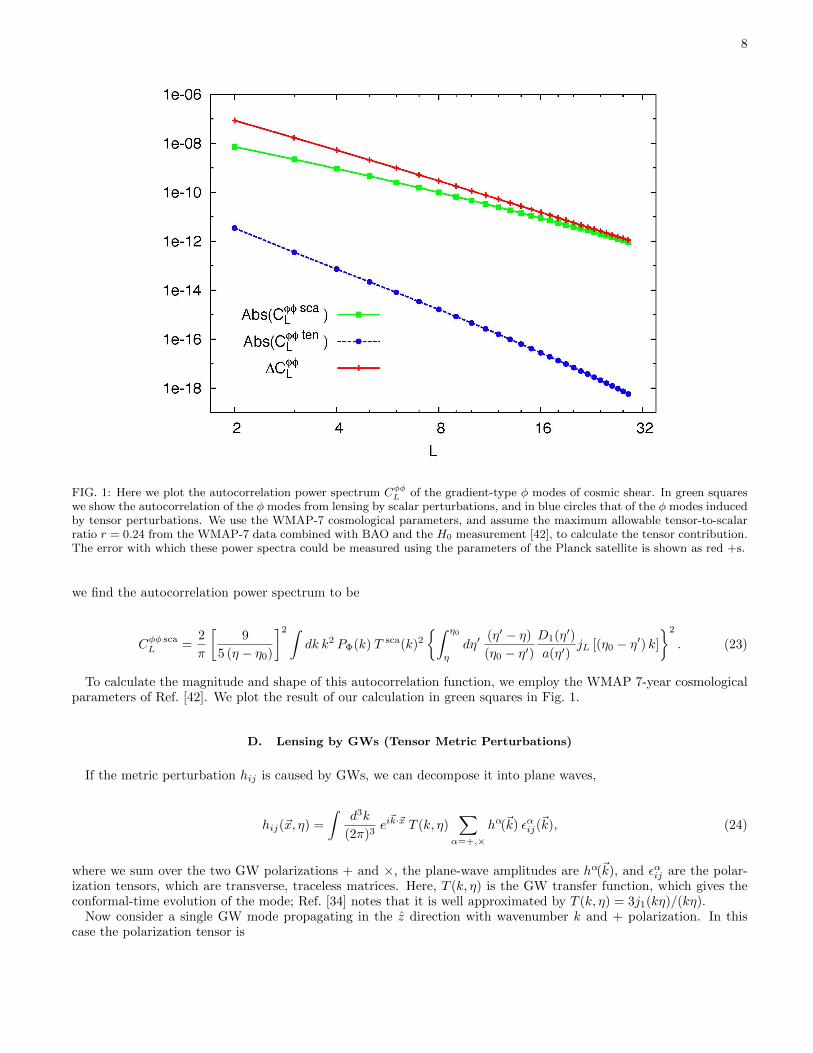
FIG. 1: Here we plot the autocorrelation power spectrum CφφL of the gradient-type φ modes of cosmic shear. In green squareswe show the autocorrelation of the φ modes from lensing by scalar perturbations, and in blue circles that of the φ modes inducedby tensor perturbations. We use the WMAP-7 cosmological parameters, and assume the maximum allowable tensor-to-scalarratio r = 0.24 from the WMAP-7 data combined with BAO and the H0 measurement [42], to calculate the tensor contribution.The error with which these power spectra could be measured using the parameters of the Planck satellite is shown as red +s.

we find the autocorrelation power spectrum to be

Cφφ scaL =

2

π

[9

5 (η − η0)

]2 ∫dk k2 PΦ(k) T sca(k)2

∫ η0

η

dη′(η′ − η)

(η0 − η′)D1(η′)

a(η′)jL [(η0 − η′) k]

2

. (23)

To calculate the magnitude and shape of this autocorrelation function, we employ the WMAP 7-year cosmologicalparameters of Ref. [42]. We plot the result of our calculation in green squares in Fig. 1.

D. Lensing by GWs (Tensor Metric Perturbations)

If the metric perturbation hij is caused by GWs, we can decompose it into plane waves,

hij(~x, η) =

∫d3k

(2π)3ei~k·~x T (k, η)

∑α=+,×

hα(~k) εαij(~k), (24)

where we sum over the two GW polarizations + and ×, the plane-wave amplitudes are hα(~k), and εαij are the polar-ization tensors, which are transverse, traceless matrices. Here, T (k, η) is the GW transfer function, which gives theconformal-time evolution of the mode; Ref. [34] notes that it is well approximated by T (k, η) = 3j1(kη)/(kη).

Now consider a single GW mode propagating in the z direction with wavenumber k and + polarization. In thiscase the polarization tensor is

9

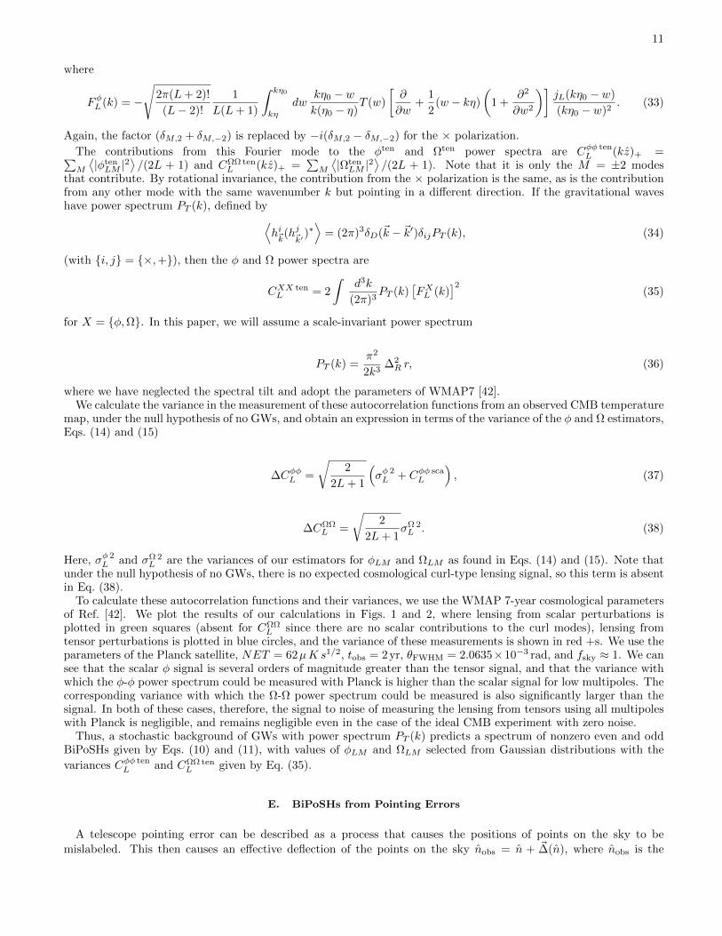
FIG. 2: Here we plot the autocorrelation power spectrum CΩΩL of the curl-type Ω modes of the weak lensing of the CMB

temperature field. These modes can only be induced by tensor perturbations. We show the signal in blue circles and the errorwith which they could be measured using the parameters of the Planck satellite as red +s.

ε+ij(kz) =

1 0 00 −1 00 0 0

.

The only non-zero metric-perturbation components are then hxx = −hyy = h+(~k) eikz T (k, η). The unit vectorn = (sin θ cosϕ, sin θ sinϕ, cos θ). The curl component of lensing of the CMB by tensor perturbations is then

∇2~θ

Ωten(n) = ikh+(~k) sin2 θ sin 2ϕ

∫ η0

η

dη′ T (k, η′)eik(η0−η′) cos θ. (25)

A GW with the × polarization is the same as that with the + polarization, but rotated by 45 to the right. TheΩten(n) pattern is therefore the same, but with sin 2ϕ replaced by − cos 2ϕ. We thus see that lensing by GWs will

give rise to nonvanishing ALMll′ .

The gradient component of cosmic shear due to tensor perturbations is a bit more complicated; it is

∇2~θφten(n) = − h

+(~k)

η0 − ηsin2 θ cos 2ϕ

∫ η0

η

dη′ T (k, η′)

3− 2ik(η′ − η) cos θ

+ (η0 − η′)[ik cos θ − k2

2(η′ − η) sin2 θ

]eik(η0−η′) cos θ. (26)

This can be further simplified by noting that

− ik cos θeik(η0−η′) cos θ =∂

∂η′eik(η0−η′) cos θ,

10

which then leads to

∇2~θφten(n) = − h

+(~k)

η0 − ηsin2 θ cos 2ϕ

∫ η0

η

dη′ T (k, η′)

3 + 2 (η′ − η)

∂

∂η′

− (η0 − η′)[∂

∂η′+

(η′ − η)

2

(k2 +

∂2

∂η′2

)]eik(η0−η′) cos θ.

(27)

For the × polarization, we replace cos 2ϕ by sin 2ϕ.Note that the expressions for ∇2

~θφten and ∇2

~θΩten differ only in two ways: (1) The curl mode has a sin 2ϕ

dependence on the azimuthal angle ϕ, while the scalar mode has a cos 2ϕ dependence (for the + polarization). (2)The η′ dependences of the two integrands differ.

We now find the spherical-harmonic coefficients φtenLM =

∫d2n φten(n)Y ∗LM (n) and Ωten

LM =∫d2nΩten(n)Y ∗LM (n).

Taking the angular derivatives of this decomposition of the curl component, we find the result Eq. (21). We also

expand these coefficients in terms of their polarization and ~k modes,

ΩtenLM =

∫d3k

(2π)3

∑α=+,×

ΩtenαLM (~k). (28)

If we consider just one mode, with α = + and ~k = kz, and use Eq. (25), its amplitude simplifies into an angular anda conformal time integral:

Ωten +LM (kz) = − ik h+(~k)

L(L+ 1)

∫ η0

η

dη′ T (k, η′)

∫d2n Y ∗LM (n) sin2θ sin(2φ) eik(η0−η′) cos θ.

The azimuthal integral is easily taken once the spherical harmonic is decomposed as

Y ∗LM (n) =

√2L+ 1

4π

(L−M)!

(L+M)!e−iMφ PLM (cos θ),

and yields the result that only M = ±2 modes remain. The polar integral can then be taken by using the partial-wavedecomposition Eq. (22) and by converting associated Legendre polynomials into regular Legendre polynomials andusing their orthogonality. The final result that we obtain for the spherical-harmonic coefficients of the curl mode is

Ωten +LM (kz) = iLh+(~k) (δM,2 − δM,−2)

√2L+ 1

2FΩL (k), (29)

where

FΩL (k) =

√2π(L+ 2)!

(L− 2)!

1

L(L+ 1)

∫ kη0

kη

dw T (w)jL(kη0 − w)

(kη0 − w)2(30)

is a transfer function for Ω. Note that in writing Eq. (30) we have assumed that T (k, η) = T (kη), and that for the ×polarization the sin 2ϕ dependence of Ω(n) is replaced by − cos 2ϕ, so that the factor (δM,2 − δM,−2) is replaced by−i(δM,2 + δM,−2).

Likewise, noting the similarities between Eqs. (25) and (27), and decomposing φtenLM into modes as in Eq. (28)

φtenLM =

∫d3k

(2π)3

∑α=+,×

φtenαLM (~k), (31)

the result for the amplitude of the gradient mode with α = + and ~k = kz is

φten +LM (kz) = iLh+(~k)(δM,2 + δM,−2)

√2L+ 1

2FφL (k), (32)

11

where

FφL (k) = −

√2π(L+ 2)!

(L− 2)!

1

L(L+ 1)

∫ kη0

kη

dwkη0 − wk(η0 − η)

T (w)

[∂

∂w+

1

2(w − kη)

(1 +

∂2

∂w2

)]jL(kη0 − w)

(kη0 − w)2. (33)

Again, the factor (δM,2 + δM,−2) is replaced by −i(δM,2 − δM,−2) for the × polarization.

The contributions from this Fourier mode to the φten and Ωten power spectra are Cφφ tenL (kz)+ =∑

M

⟨|φtenLM |2

⟩/(2L + 1) and CΩΩ ten

L (kz)+ =∑M

⟨|ΩtenLM |2

⟩/(2L + 1). Note that it is only the M = ±2 modes

that contribute. By rotational invariance, the contribution from the × polarization is the same, as is the contributionfrom any other mode with the same wavenumber k but pointing in a different direction. If the gravitational waveshave power spectrum PT (k), defined by⟨

hi~k(hj~k′)∗⟩

= (2π)3δD(~k − ~k′)δijPT (k), (34)

(with i, j = ×,+), then the φ and Ω power spectra are

CXX tenL = 2

∫d3k

(2π)3PT (k)

[FXL (k)

]2(35)

for X = φ,Ω. In this paper, we will assume a scale-invariant power spectrum

PT (k) =π2

2k3∆2R r, (36)

where we have neglected the spectral tilt and adopt the parameters of WMAP7 [42].We calculate the variance in the measurement of these autocorrelation functions from an observed CMB temperature

map, under the null hypothesis of no GWs, and obtain an expression in terms of the variance of the φ and Ω estimators,Eqs. (14) and (15)

∆CφφL =

√2

2L+ 1

(σφ 2L + Cφφ sca

L

), (37)

∆CΩΩL =

√2

2L+ 1σΩ 2L . (38)

Here, σφ 2L and σΩ 2

L are the variances of our estimators for φLM and ΩLM as found in Eqs. (14) and (15). Note thatunder the null hypothesis of no GWs, there is no expected cosmological curl-type lensing signal, so this term is absentin Eq. (38).

To calculate these autocorrelation functions and their variances, we use the WMAP 7-year cosmological parametersof Ref. [42]. We plot the results of our calculations in Figs. 1 and 2, where lensing from scalar perturbations isplotted in green squares (absent for CΩΩ

L since there are no scalar contributions to the curl modes), lensing fromtensor perturbations is plotted in blue circles, and the variance of these measurements is shown in red +s. We use theparameters of the Planck satellite, NET = 62µK s1/2, tobs = 2yr, θFWHM = 2.0635×10−3 rad, and fsky ≈ 1. We cansee that the scalar φ signal is several orders of magnitude greater than the tensor signal, and that the variance withwhich the φ-φ power spectrum could be measured with Planck is higher than the scalar signal for low multipoles. Thecorresponding variance with which the Ω-Ω power spectrum could be measured is also significantly larger than thesignal. In both of these cases, therefore, the signal to noise of measuring the lensing from tensors using all multipoleswith Planck is negligible, and remains negligible even in the case of the ideal CMB experiment with zero noise.

Thus, a stochastic background of GWs with power spectrum PT (k) predicts a spectrum of nonzero even and oddBiPoSHs given by Eqs. (10) and (11), with values of φLM and ΩLM selected from Gaussian distributions with the

variances Cφφ tenL and CΩΩ ten

L given by Eq. (35).

E. BiPoSHs from Pointing Errors

A telescope pointing error can be described as a process that causes the positions of points on the sky to be

mislabeled. This then causes an effective deflection of the points on the sky nobs = n + ~∆(n), where nobs is the

12

direction that the telescope believes it is pointed in and n is its actual pointing direction. As we saw in Sec. III A,

we can decompose this deflection field ~∆(n) into gradient and curl components, which source even- and odd-parityBiPoSHs, respectively. Thus, from Eq. (17) we can see that any pointing error that has a nonzero curl component~∇~θ × ~∆(n) will excite odd-parity BiPoSHs.

Imagine, for example, that a satellite such as Planck misestimates the rate with which it is precessing. Since it isthis precession that builds up observations of subsequent rings of the sky, such a misestimation would cause a shearingof each ring relative to its neighbors. This type of a deflection has a nonzero curl component, and thus would exciteodd-parity BiPoSHs. Measurement of these BiPoSHs, and in particular the odd-parity BiPoSHs, can therefore providea useful check for such pointing errors.

IV. BIPOSHS AS PROBES OF PARITY VIOLATION

A. Correlation of Opposite-Parity Lensing Components

Since the A⊕LMll′ and A

LMll′ have opposite parity for the same L and M , a cross-correlation between the two can arise

only if there is some parity-breaking in the physics responsible for producing the departures from SI/Gaussianity. Herewe mention, by way of example, chiral GWs as a mechanism to produce such a parity-violating correlation [43–45].

The contribution to the cross-correlation power spectrum from a single Fourier mode in the z direction with +

polarization is CφΩL (kz) =

∑m 〈φLM Ω∗LM 〉 /(2L+ 1) = 0; it vanishes as the contribution from M = 2 is canceled by

that from M = −2. And if this is true, then by rotational invariance it is true for any other linearly-polarized GW.

We thus conclude that a stochastic GW background predicts CφΩL = 0. In other words, there is no cross-correlation

between φ and Ω, and thus no cross-correlation between the even and odd BiPoSHs, A⊕LMll′ and A

LMll′ .

Following Ref. [44], however, consider a right-circularly polarized GW: hR = h+ +ih× (i.e., we sum a + polarizationwave with a × polarization wave out of phase by 90). The azimuthal-angle dependence for the wave is then e2iϕ,and ΩLM and φLM have contributions only from M = 2. There is thus a nonzero cross-correlation between φ and Ω.Similarly for a left-circularly polarized GW hL = h+ − ih×, the ϕ dependence is e−2iϕ, and only M = −2 modes areexcited. There is again a cross-correlation between φ and Ω, but this time with the opposite sign.

In the standard inflationary scenario, there are equal numbers of right- and left-circularly polarized GWs, and thecross-correlation between φ and Ω therefore vanishes. But if for some reason there is an asymmetry between thenumber of right- and left-circularly polarized GWs [43–46], a manifestation of parity breaking, then there may be a

parity-violating cross-correlation between φ and Ω, and thus between A⊕LMll′ and A

LMll′ .

The chirality of the GW background can be parametrized by an amplitude A which can take values between −1and 1, where A = +1 denotes that all of the GWs are right-circularly polarized, and A = −1 denotes that they areall left-circularly polarized. But we have seen that a right-handed GW contributes only to M = 2 modes, while aleft-handed one contributes only to M = −2. We can denote this by weighting M = 2 components by (A+ 1)/2 andM = −2 components by (A− 1)/2, so that our version of Eq. (29), for example, that is appropriate to the case of achiral GW background will be

Ωten +LM (kz) = iLh+(~k)

[(1 +A)

2δM,2 −

(1−A)

2δM,−2

]√2L+ 1

2FΩL (k), (39)

and similarly for Eq. (32). In this way a fully right circularly-polarized GW background will have only contributionsfrom M = 2, a fully left-circularly polarized background will have only contributions from M = −2, and if the amountof left and right-circularly polarized waves is equal, that is if the GW background is non-chiral, the contributions fromM = 2 and M = −2 cancel. The φ-Ω cross-correlation power spectrum is given by

CφΩL = A

∫d3k

(2π)3PT (k)FφL (k)FΩ

L (k). (40)

Refs. [34, 36, 47] have shown that the amplitude of the stochastic gravitational-wave background is probably toosmall, even with the most optimistic assumptions, to produce a detectable gravitational-lensing signal in the CMB.The example of a chiral gravitational-wave background as a possible source of a detectable parity-breaking BiPoSHcorrelation is principally of academic interest. Still, Ref. [35] has recently argued that weak lensing of the CMB by GWsmay be detectable in its cross-correlation with the CMB-polarization pattern induced by these GWs [37, 38, 48–50].We thus surmise that a chiral gravitational-wave background may still be able produce a detectable parity-breakingsignal in BiPoSHs in cross-correlation with the CMB polarization, an idea we explore in the next section.

13

B. Large-Angle CMB Polarization Spectra

We follow the work of Ref. [35], finding the multipole moments of the CMB E- and B-type polarization spectra forlarge angular scales by considering only those modes that are produced after reionization. The spherical-harmoniccoefficients of B-type polarization modes can be decomposed as

Blm =

∫d3k

(2π)3

∑α=+,×

Bαlm(~k), (41)

where Bαlm(~k) is the amplitude of polarization B modes multipole moment lm in the direction ~k. The general form ofthis amplitude is quite complicated, but we can simplify it if, as in Sec. III D, we consider only a single, +-polarizedGW traveling in the z direction with wavenumber k. In this case, the B-mode amplitude can be written

B+lm(kz) = il hα(~k) (δm,2 − δm,−2)

√2l + 1

2FBl (k), (42)

FBl (k) =1

2l + 1

√9π

2

∫ η0

ηre

dη τ(η) (l + 2)jl−1[k(η0 − η)]− (l − 1)jl+1[k(η0 − η)]∫ kη

kηlss

dx−3 j2(x)

x

j2(kη − x)

(kη − x)2,

(43)

where the hα(~k) are the amplitudes of GW modes as defined in Eq. (24), τ(η) is the scattering rateτ(η) = ne(η) σT a(η), with ne the electron density, σT the Thompson scattering cross-section, and a the scalefactor, and ηre and η0 are the conformal times at reionization and today, respectively. Since we are only interested insmall scales, we find the approximation ηlss = 0 is sufficient for our purposes, making the last integral significantlyfaster to evaluate. The result above agrees with the results of Ref. [35], whose method we followed in its derivation,up to a factor of i.

We find that the corresponding E-type polarization multipoles from tensor perturbations take the same form asBlm above, except for the opposite sign in front of δm,−2 and a different factor in the curly brackets in Eq. (43).From Ref. [49] we find this alternative form to be (2l + 1)/2

−jl(x) + j′′l (x) + 2jl(x)/x2 + 4j′l(x)/x

, where here

x = [k(η0 − η)], and derivatives are with respect to x. Employing spherical Bessel function identities, we can thenwrite the E-type polarization multipoles as

Elm =

∫d3k

(2π)3

∑α=+,×

Eαlm(~k), (44)

E+lm(kz) =il hα(~k) (δm,2 + δm,−2)

√2l + 1

2FEl (k), (45)

FEl (k) =1

2l + 1

√9π

2

∫ η0

ηre

dη τ(η)

(2l + 1)

[k(η0 − η)]2jl[k(η0 − η)]− (2l + 1)(3l2 + 3l − 4)

(2l − 1)(2l + 3)jl[k(η0 − η)]

+l(l + 3)

2(2l − 1)jl−2[k(η0 − η)] +

(l + 1)(l − 2)

2(2l + 3)jl+1[k(η0 − η)]

∫ kη

kηlss

dx−3 j2(x)

x

j2(kη − x)

(kη − x)2, (46)

where the terms are defined as they were above for the Blm amplitudes.

C. Parity-Violating Correlations from Chiral GWs

We now want to calculate the expected cross-correlation between CMB-polarization multipole coefficients and weak-lensing-induced BiPoSHs of opposite parity. Note that these cross-correlations are directly related to the parity-oddthree-point correlations discussed in Ref. [51]. As we mentioned above, if there is no parity-violating physics, thenin the cross-correlation of a parity-even and a parity-odd observable, M = 2 terms and M = −2 terms will canceleach other, giving a net zero cross-correlation. However, if for example the GW background is chiral, then parity isbroken and we can get a non-zero cross-correlation between opposite parity observables. As we saw in Sec. IV A, aright-handed GW contributes only to M = 2 modes, while a left-handed one contributes only to M = −2. If we carryout a similar procedure for Eqs. (42), and (45) as we did in Eq. (39), weighting M = 2 components by (A+ 1)/2 and

14

FIG. 3: Here we plot the cross-correlation CφBL between the gradient φ modes of the weak lensing of cosmic shear with thecurl-type B modes of the CMB polarization in blue circles, and the noise on this measurement due to cosmic variance andPlanck satellite instrumental noise in red +s. Since these quantities are of opposite parity, in the absence of parity-breakingphysics we expect this cross-correlation to vanish. However, if we assume for example that the entire allowable GW backgroundis right-circularly polarized, such a cross-correlation could occur. The cross-correlation is linearly proportional to the chiralityparameter A, defined such that A = 1 denotes a completely right-circularly polarized GW background, A = −1 denotescompletely left-circularly polarized, and A = 0 denotes an unpolarized background. Here we assume the maximum allowabletensor-to-scalar ratio r = 0.24, the limit from WMAP-7 data combined with BAO and the H0 measurement [42]. Cusps in theabsolute value of the correlation function correspond to sign changes of the correlation function.

M = −2 components by (A − 1)/2, we can calculate parity-violating correlations between polarization and lensingcomponents while accounting for the amplitude and handedness of a chiral GW background.

First considering the cross-correlation between B-modes of the CMB polarization and gradient-type modes of cosmicshear, we write

CφBL =1

2L+ 1

∑M

〈φLMB∗LM 〉.

As before, by rotational invariance we know that both + and × polarizations will contribute equally to CφBL , as will

modes with any wavenumber ~k whose magnitude k is the same. We can see that only φtenLM will contribute to this

correlation, and not φscaLM , as the scalar perturbation field is not correlated, on average, with the tensor perturbation

field. Then using Eqs. (31), (32), (34), (41) and (42), we can write this cross-correlation as

CφBL = A

∫d3k

(2π)3PT (k) FφL (k) FBL (k). (47)

Similarly, we can write the cross-correlation between E-type polarization modes and curl-type modes of cosmicshear, using Eqs. (28), (29), (34), (44), and (45), as

15

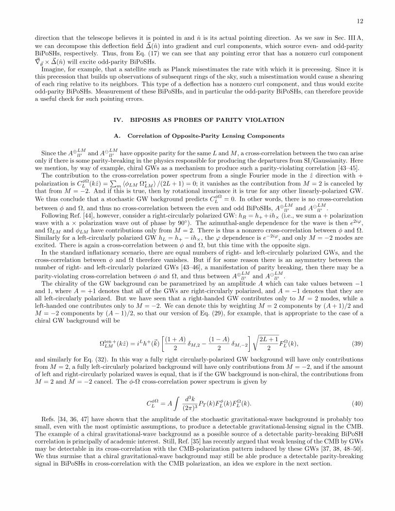
FIG. 4: Here we plot the cross-correlation CΩEL between the curl-type Ω modes of cosmic shear with the gradient-type E-

modes of the CMB polarization in blue circles, and the noise on this measurement due to cosmic variance and Planck satelliteinstrumental noise in red +s. As with the φ−B correlation, we assume a completely right-circularly polarized GW background,with the maximum currently permitted tensor-to-scalar ratio.

CΩEL = A

∫d3k

(2π)3PT (k) FΩ

L (k) FEL (k), (48)

where the GW power spectrum is given by

PT (k) =π2 r ∆2

R(k0)

2 k3.

We want to calculate the magnitude and shape of such correlations, to determine whether such a signal is observable.We use the WMAP 7-year cosmological parameters and assume the maximum allowable level of GWs from earlyuniverse physics, with a tensor-to-scalar ratio r = 0.24, the limit from the WMAP-7 data combined with BAO andthe H0 measurement [42]. We also assume that the GW background is entirely right-circularly polarized. As a firstestimate, we calculate the level of such correlations while making several assumptions. We use the approximate formof the GW transfer function T (k, η) ' 3j1(kη)/(kη), assume that reionization happened instantaneously so that theelectron density ne is equal to a step function, and neglect contributions to the polarization modes that came fromlast scattering. The two last assumptions affect mostly the higher-L multipoles, which in this cross-correlation aresuppressed since we see that φten

LM and ΩtenLM fall off very fast with L.

With these assumptions, we have calculated the correlation functions CφBL and CΩEL , and show them as the blue

circles in Figs. 3 and 4. Note that the absolute value of the correlation functions are plotted, and that the cusps in theprofiles result from sign changes. Note also that both correlation functions are linearly proportional to the chiralityparameter A, so that they would flip in sign if the GW background were left instead of right-circularly polarized. Weare only interested in low multipoles, since our assumptions break down for larger L, and such multipoles are stronglysuppressed in correlation with the weak-lensing modes.

16

D. Variance of φ-B and Ω-E Correlations

It is useful to know the variance with which we could measure such parity-violating cross-correlations. From Ref. [37]we see that the variance with which we could measure the cross-correlation CXYL of two distinct Gaussian randomvariables X and Y is given by

(∆CXYL

)2 ≡ ⟨(CXYL − CXYL)2⟩,

where CXYL = 1/(2L + 1)∑M XLMY

∗LM is the estimator for the cross-correlation, and CXYL is its theoretical value

under the null hypothesis. Ref. [37] then evaluates this variance, assuming distinct X and Y , to be

(∆CXYL

)2=

1

2L+ 1

[(CXYL

)2+ CXX map

L CY Y mapL

], (49)

where, as before, CXX mapL = W 2

LCL +NXXL , with WL the window function defined in Sec. II C, and NXX

L the noisein the measurement of CXXL .

In our case, the null hypothesis is that there is a GW background with the maximal tensor-to-scalar ratio, but itcontains equal numbers of right- and left-circularly polarized GWs, i.e., it is not chiral. In this case, the theoreticalvalue of parity-violating cross-correlations is zero, so that the first term in Eq. (49) vanishes. Then, assuming that

φLM and ΩLM are Gaussian random variables, a reasonable assumption since many uncorrelated noise processes arelikely to contribute to this measured value, we find for the variances,

(∆CφBL

)2

=1

2L+ 1CφφmapL CBBmap

L (50)(∆CΩE

L

)2

=1

2L+ 1CΩΩ mapL CEEmap

L . (51)

To calculate these errors, we know that the instrumental errors on the polarization power spectra are given by

NEEL = NBB

L =8π(NET)2

tobs

√fsky

.

We use the Planck-satellite parameters, as in Sec. III D. We also use the CMB anisotropy calculator CAMB to calculatethe temperature and polarization power spectra including effects at the surface of last scatter [52]. The resulting errorsare shown as red +s in Figs. 3 and 4. This noise, which combines instrumental and cosmic-variance sources, is atleast an order of magnitude above the corresponding maximum signal level at low multipoles, and drops less rapidlywith l so that the low multipoles yield the highest signal-to-noise.

E. Signal-to-Noise Ratio of Chiral GW Background Detection

We finally wish to calculate the achievable signal-to-noise of a measurement of the magnitude of such cross-correlations given our calculations of their shapes and variances. Such a measurement would tell us about thepresence or absence of a chiral GW background, or of parity violation in the processes that caused departures fromGaussianity/SI in general. We can phrase the aim of this calculation as finding the error with which we could measurethe chirality parameter A, which sets the amplitude of the cross-correlations relative to their maximum values in thecase of a completely circularly polarized GW background, as in Eqs. (47) and (48). Let us calculate this for the caseof the φ-B cross-correlation; the Ω-E case will be similar.

We define a new quantity CφBLmax, defined such that

CφBL = A CφBLmax.

17

If we assume that the instrumental noise on CφBL is Gaussian, so that CφBL ≡ W−2L CφBL is a random variable drawn

from a Gaussian probability distribution with variance(

∆CφBL

)2

and mean A CφBLmax, we can find the maximum-

likelihood estimator for A to be

A =

∑L C

φBL CφBLmax

(∆CφBL

)−2

∑L

(CφBLmax

)2 (∆CφBL

)−2 .

Then, assuming that the instrumental noise is uncorrelated between different multipoles, the variance of this estimatoris given by

⟨A2⟩

=

[∑L

(CφBLmax

)2 (∆CφBL

)−2]−1

.

The maximum signal-to-noise with which we can measure this amplitude is given by

(S

N

)φBmax

=Amax√⟨A2⟩ =

[∑L

(CφBLmax

)2 (∆CφBL

)−2]1/2

. (52)

The same method can be used to calculate the obtainable signal-to-noise from the Ω-E cross correlation, giving

(S

N

)ΩE

max

=

[∑L

(C ΩELmax

)2 (∆C ΩE

L

)−2

]1/2

. (53)

Using the values of the cross-correlations and their errors calculated above, we find that the obtainable signal-to-

noise from measurement of these cross-correlations is 0.002 for CΩEL and 0.01 for CφBL . These numbers are too small for

us to have any reasonable expectation of detection using the Planck satellite. Recalculating the above errors assumingan ideal CMB experiment, with no instrumental noise and infinite resolution, the values of the signal-to-noise onlychange by a factor of two, indicating that this method is not likely to be a promising way to detect a chiral GWbackground.

V. CONCLUSIONS

BiPoSHs are a formalism to describe correlations between two different spherical-harmonic coefficients of the CMBtemperature field, which can occur if the CMB temperature field is not exactly Gaussian or statistically isotropic.This paper introduces odd-parity BiPoSHs, a set of BiPoSHs that has not yet been studied, and details how they canbe estimated from knowledge of the CMB temperature fluctuations.

We calculate the even- and odd-parity BiPoSHs that are sourced by gradient- and curl-type deflections of the CMB,respectively, and from this we obtain estimators for these deflections in terms of the BiPoSH coefficients. We showthat lensing by scalar metric perturbations causes only gradient-type deflections, and thus only sources even-parityBiPoSHs. However, lensing by GWs produces both gradient- and curl-type deflections and thus sources both even- andodd-parity BiPoSHs. We calculate the expected power spectra of deflections due to scalar and tensor perturbationsand their errors, and conclude that a reasonable signal-to-noise measurement of the amplitude of the GW backgroundcannot be obtained from these autocorrelations even with the ideal CMB experiment, and thus from autocorrelationsof the BiPoSH coefficients.

Although lensing by GWs produces both even- and odd-parity BiPoSHs, their opposite parity implies that theycould not be correlated. However, in the presence of parity-violating physics, such as a chiral GW background, thisparity argument breaks down and we might expect a correlation. We consider such a cross-correlation, and encourageits measurement even though the likelihood of observing a cosmological signal is low.

A GW background also produces signals in the E- and B-type CMB polarization spectra, which are of even andodd parity, respectively. We consider the possibility that a chiral GW background would produce cross-correlations

18

between opposite-parity components of lensing and polarization, and calculate the expected magnitude and errors ofsuch cross-correlations. Although we find that the likelihood of observing a cosmological signal is low, we encouragethe measurement of these cross-correlations since such a detection would provide evidence of important systematicerrors or even new parity-breaking physics.

Here we have discussed BiPoSHs constructed from temperature multipole moments only, but the formalism canbe generalized to include the polarization as well. It may also be that inclusion of the polarization improves thesensitivity to these parity-breaking, and other, signals. We plan to pursue this analysis in future work.

Finally, we note that weak-lensing distortions of distant galaxies can also be decomposed into curl and gradientcomponents [32, 53]. Similar tests for parity violation can thus also be carried out with weak lensing of galaxies.

Acknowledgments

LGB thanks Esfandiar Alizadeh, Christopher Hirata and Fabian Schmidt for useful discussions, and acknowledgesthe support of the NSF Graduate Research Fellowship Program. MK thanks the support of the Miller Institute forBasic Research in Science and the hospitality of the Department of Physics at the University of California, Berkeley,where part of this work was completed. This work was supported at Caltech by DoE DE-FG03-92-ER40701, NASANNX10AD04G, and the Gordon and Betty Moore Foundation. TS acknowledges support from Swarnajayanti grant,DST, India and the visit to Caltech during which the work was carried out.

[1] G. F. Smoot et al., Astrophys. J. 396, L1 (1992).[2] A. Lewis and A. Challinor, Phys. Rept. 429, 1 (2006) [arXiv:astro-ph/0601594].[3] S. M. Carroll, G. B. Field and R. Jackiw, Phys. Rev. D 41, 1231 (1990).[4] R. R. Caldwell, V. Gluscevic and M. Kamionkowski, arXiv:1104.1634 [astro-ph.CO].[5] F. K. Hansen, A. J. Banday and K. M. Gorski, Mon. Not. Roy. Astron. Soc. 354, 641 (2004) [arXiv:astro-ph/0404206].[6] A. de Oliveira-Costa, M. Tegmark, M. Zaldarriaga and A. Hamilton, Phys. Rev. D 69, 063516 (2004) [arXiv:astro-

ph/0307282].[7] D. Hanson and A. Lewis, Phys. Rev. D 80, 063004 (2009) [arXiv:0908.0963 [astro-ph.CO]].[8] L. Verde, L. M. Wang, A. Heavens and M. Kamionkowski, Mon. Not. Roy. Astron. Soc. 313, L141 (2000) [arXiv:astro-

ph/9906301].[9] E. Komatsu and D. N. Spergel, Phys. Rev. D 63, 063002 (2001) [arXiv:astro-ph/0005036].

[10] M. Kunz, A. J. Banday, P. G. Castro, P. G. Ferreira and K. M. Gorski, arXiv:astro-ph/0111250.[11] A. Hajian and T. Souradeep, Astrophys.J. 597, L5,(2003) [arXiv:astro-ph/0308001][12] A. Hajian and T. Souradeep, arXiv:astro-ph/0501001.[13] N. Joshi, S. Jhingan, T. Souradeep and A. Hajian, Phys. Rev. D 81, 083012 (2010) [arXiv:0912.3217 [astro-ph.CO]].[14] A. Hajian and T. Souradeep, arXiv:astro-ph/0301590.[15] A. R. Pullen and M. Kamionkowski, Phys. Rev. D 76, 103529 (2007) [arXiv:0709.1144 [astro-ph]].[16] A. Hajian, T. Souradeep and N. J. Cornish, Astrophys. J. 618, L63 (2004) [arXiv:astro-ph/0406354].[17] T. Souradeep and A. Hajian, Pramana 62, 793 (2004) [arXiv:astro-ph/0308002].[18] T. Souradeep, A. Hajian and S. Basak, New Astron. Rev. 50, 889 (2006) [arXiv:astro-ph/0607577].[19] A. Hajian and T. Souradeep, Phys. Rev. D 74, 123521 (2006) [arXiv:astro-ph/0607153].[20] T. Ghosh, A. Hajian and T. Souradeep, Phys. Rev. D 75, 083007 (2007) [arXiv:astro-ph/0604279].[21] S. Basak, A. Hajian and T. Souradeep, Phys. Rev. D 74, 021301 (2006) [arXiv:astro-ph/0603406].[22] D. Hanson, A. Lewis and A. Challinor, Phys. Rev. D 81, 103003 (2010) [arXiv:1003.0198 [astro-ph.CO]].[23] C. L. Bennett et al., arXiv:1001.4758 [astro-ph.CO].[24] M. Kamionkowski, Phys. Rev. Lett. 102, 111302 (2009) [arXiv:0810.1286 [astro-ph]].[25] V. Gluscevic, M. Kamionkowski and A. Cooray, Phys. Rev. D 80, 023510 (2009) [arXiv:0905.1687 [astro-ph.CO]].[26] A. P. S. Yadav, R. Biswas, M. Su and M. Zaldarriaga, Phys. Rev. D 79, 123009 (2009) [arXiv:0902.4466 [astro-ph.CO]].[27] T. Souradeep, Indian J. Phys. 80, 1063 (2006) [arXiv:gr-qc/0609026].[28] M. Aich and T. Souradeep, Phys. Rev. D 81, 083008 (2010) [arXiv:1001.1723 [astro-ph.CO]].[29] T. Souradeep and A. Hajian, arXiv:astro-ph/0502248.[30] L. Ackerman, S. M. Carroll and M. B. Wise, Phys. Rev. D 75, 083502 (2007) [arXiv:astro-ph/0701357].[31] W. Hu, Pys. Rev. D 62, 043007 (2000) [arXiv:astro-ph/0001303].[32] A. Stebbins, arXiv:astro-ph/9609149.[33] N. Kaiser and A. H. Jaffe, Astrophys. J. 484, 545 (1997) [arXiv:astro-ph/9609043].[34] S. Dodelson, E. Rozo and A. Stebbins, Phys. Rev. Lett. 91, 021301 (2003) [arXiv:astro-ph/0301177].[35] S. Dodelson, Phys. Rev. D 82, 023522 (2010) [arXiv:1001.5012 [astro-ph.CO]].[36] C. Li and A. Cooray, Phys. Rev. D 74, 023521 (2006) [arXiv:astro-ph/0604179].

19

[37] M. Kamionkowski, A. Kosowsky and A. Stebbins, Phys. Rev. D 55, 7368 (1997) [arXiv:astro-ph/9611125].[38] M. Kamionkowski, A. Kosowsky and A. Stebbins, Phys. Rev. Lett. 78, 2058 (1997) [arXiv:astro-ph/9609132].[39] L. G. Book, E. E. Flanagan, Phys. Rev. D83, 024024 (2011). [arXiv:1009.4192 [astro-ph.CO]].[40] S. Dodelson, Amsterdam, Netherlands: Academic Pr. (2003) 440 p.[41] J. M. Bardeen, J. R. Bond, N. Kaiser, A. S. Szalay, Astrophys. J. 304, 15-61 (1986).[42] E. Komatsu et al. [ WMAP Collaboration ], Astrophys. J. Suppl. 192, 18 (2011). [arXiv:1001.4538 [astro-ph.CO]].[43] C. R. Contaldi, J. Magueijo and L. Smolin, Phys. Rev. Lett. 101, 141101 (2008) [arXiv:0806.3082 [astro-ph]].[44] A. Lue, L. M. Wang and M. Kamionkowski, Phys. Rev. Lett. 83, 1506 (1999) [arXiv:astro-ph/9812088].[45] T. Takahashi and J. Soda, Phys. Rev. Lett. 102, 231301 (2009) [arXiv:0904.0554 [hep-th]].[46] V. Gluscevic and M. Kamionkowski, Phys. Rev. D 81, 123529 (2010) [arXiv:1002.1308 [astro-ph.CO]].[47] A. Cooray, M. Kamionkowski and R. R. Caldwell, Phys. Rev. D 71, 123527 (2005) [arXiv:astro-ph/0503002].[48] P. Cabella and M. Kamionkowski, arXiv:astro-ph/0403392.[49] J. R. Pritchard and M. Kamionkowski, Annals Phys. 318, 2 (2005) [arXiv:astro-ph/0412581].[50] M. Zaldarriaga and U. Seljak, Phys. Rev. D 55, 1830 (1997) [arXiv:astro-ph/9609170]; U. Seljak and M. Zaldarriaga, Phys.

Rev. Lett. 78, 2054 (1997) [arXiv:astro-ph/9609169].[51] M. Kamionkowski and T. Souradeep, Phys. Rev. D 83, 027301 (2011) [arXiv:1010.4304 [astro-ph.CO]].[52] http://camb.info/

[53] M. Kamionkowski, A. Babul, C. M. Cress and A. Refregier, Mon. Not. Roy. Astron. Soc. 301, 1064 (1998) [arXiv:astro-ph/9712030].