1

OECD REGIONAL TYPOLOGY

June 2011

Directorate for Public Governance and Territorial Development

2

TABLE OF CONTENTS

OECD REGIONAL TYPOLOGY .................................................................................................................. 3

Methodology to classify regions into predominantly urban, intermediate or predominantly rural ............. 3 Extension to rural regions clos to a city and remote rural regions ............................................................... 5 Annex: Data inputs for the extension of the OECD regional typology ....................................................... 9

Accessibility Analysis ............................................................................................................................ 10 Distribution of the population ................................................................................................................ 10 Road Network ........................................................................................................................................ 11 Populated Centres ................................................................................................................................... 11 Additional factors ................................................................................................................................... 11 Service Areas.......................................................................................................................................... 12

Tables

Table 1. Local units of OECD countries ............................................................................................... 4 Table 2. Number of regions and percentage of population by typology based on 90 minutes of

driving time, Mexico .................................................................................................................................. 14

Figures

Figure 1. OECD Regional typology - North America ............................................................................ 6 Figure 2. OECD regional typology - Europe .......................................................................................... 7 Figure 3. OECD Regional typology - Asia ............................................................................................. 8 Figure 4. Elements for the accessibility analysis .................................................................................. 13 Figure 5. Service areas for 30-min, 60-min and 90-min time frames, North America ......................... 15

3

OECD REGIONAL TYPOLOGY

Methodology to classify regions into predominantly urban, intermediate or predominantly rural

Regions of OECD member countries have been classified into Predominantly Urban, Intermediate and

Predominantly Rural to take into account geographical differences among them. Comparing the socio-

economic performance of regions of the same type (whether urban or rural) across countries is useful in

detecting similar characteristics and development paths. This typology has been used by the OECD in its

analytical work (see, for example, the series OECD Regions at a Glance1), as well as in analysis carried

out by other institutions, such as National Statistical Offices and the European Commission.

The OECD regional typology is applied only to regions at Territorial Level 3 (TL3) and it is based on

criteria of population density and size of the urban centres located within a region.

The methodology is made of three main steps:

1. The first step of the methodology consists in classifying “local units” (administrative entities at a

geographical level lower than TL3) (Table 1) as rural if their population density is below 150

inhabitants per square kilometre (500 inhabitants for Japan and Korea, to account for the fact

that its national population density exceeds 300 inhabitants per square kilometre).2

2. The second step consists in aggregating this lower level (local units) into TL3 regions and

classifying the latter as “predominantly urban”, “intermediate” and “predominantly rural” using

the percentage of population living in rural local units (local units with a population density

below 150 inhabitants per square kilometre). TL3 regions are then classified as:

Predominantly Urban (PU), if the share of population living in rural local units is below

15%;

Intermediate (IN), if the share of population living in rural local units is between 15% and

50%;

Predominantly Rural (PR), if the share of population living in rural local units is higher

than 50%

3. Finally, a third step takes into acoount the size of the urban centres contained in the TL3 regions,

and adjusts the classification based on the following rules:

A region classified as predominantly rural by steps 1 and 2 becomes intermediate if it

contains an urban centre of more than 200 000 inhabitants (500 000 for Japan and Korea)

representing at least 25% of the regional population.

A region classified as intermediate by steps 1 and 2 becomes predominantly urban if it

contains an urban centre of more than 500 000 inhabitants (1 000 000 for Japan and Korea)

representing at least 25% of the regional population

1 . “OECD Regions at a Glance”; OECD Publishing 2007, 2009 and 2011 editions

www.oecd.org/regional/regionsataglance

2 . The population and area data for Local Units are for the census year 2000-2001.

4

Table 1. Local units of OECD countries

Country Local units Australia Statistical Local Areas (SLA) - ABS Austria Gemeinden (LAU2) Belgium Gemeenten/Communes (LAU2) Canada Census Consolidated Subdivision – Statistics Canada Czech Republic Obce (LAU2) Denmark Municipalities (before reform) Finland Kunnat/Kommuner (LAU2) France Communes (LAU2) Germany Verbandsgemeinden Greece Dimoi/Koinotites (LAU1) Hungary Települések (LAU2) Iceland Municipalities Ireland Electoral Districts (LAU2) Italy Comuni (LAU2) Japan Municipalities (as of 1999) Korea Counties Luxembourg Communes (LAU2) Mexico Municipios Netherlands Gemeenten (LAU2) New Zealand Area Units (Stat. New Zealand) Norway Municipalities Poland Gminy (LAU2) Portugal Freguesias (LAU2) Slovak Republic Obce (LAU2) Spain Municipios (LAU2) Sweden Kommuner (LAU2) Switzerland Municipalities Turkey Districts United Kingdom Wards (or parts thereof) (LAU2) United States Counties

Urban centres in the third criterion are defined by population density and size, not by functional

criteria such as commuting. For example, in the United States the third criterion considers the population

size of urban centres according to the definition of “Urban Areas” (UAs)3 and not according to the

definition of the Metropolitan Statistical Areas (MSAs).4 The choice of giving explicit weight to the

population density criterion is based on the assumption that functional urban areas might include in their

territories areas that are not densely populated.

A second issue arises when the urban centre is bigger than the local unit or when the urban centre is

not entirely contained by the local unit defined in the first step. This can create problems in the

identification of the urban centre itself, like in the cases of Finland and Turkey:

In Turkey the regions concerned were Izmir, Ankara, Konia and Kayseri. Konia was upgraded

from PR to IN, and the remaining four from IN to PU. In Ankara for instance, the population of

the city of Ankara is concentrated in a few neighbouring local units (districts): Etimesgut,

3. Urban areas in the United States are defined by the U.S. Census Bureau as contiguous census block groups

with a population density of at least 1,000 per square mile (about 400 per square km). Urban areas are

delineated without regard to political boundaries. Urban areas with a population of at least 50,000 serve as

the core of a metropolitan statistical area. Urban areas are among the most accurate measure of a city's true

size, due to the fact that they are all measured from the same criteria.

4. MSAs are delineated on the basis of a central urbanized area—a contiguous area of relatively high

population density. The counties containing the core urbanized area are known as the central counties of

the MSA. Additional surrounding counties (known as outlying counties) can be included in the MSA if

these counties have strong social and economic ties to the central counties as measured by commuting and

employment. Note that some areas within these outlying counties may actually be rural in nature.

5

Yenimahalle, Cankaya and Keçiören. None of these districts individually meets both the

population size criteria (higher than 500 000) or the concentration criteria (25% of the regional

population). Therefore, even if its urban centre altogether meets the additional criterion, Ankara

would not be upgraded to Predominantly Urban because its centre is split/hidden into four

different local units.

In Finland the region concerned was Pirkanmaa. The municipality containing Tampere had about

195 000 inhabitants in 2001. According to the additional criterion, the population size was not

enough to upgrade the region from PR to IN, although the percentage of population living in the

Tampere municipality reached the 44% of the total regional population. Like in the case of

Ankara the Tampere municipality did not contain the whole urban area of the city of Tampere

which is spread across other municipalities surrounding it.

In both cases the joint work between the OECD Secretariat and the WPTI Delegates has allowed for a

more accurate implementation of the criterion based on the size of urban centres. The OECD regional

Typology can be downloaded in different electronic formats from the OECD data warehouse OECD.Stat5.

Extension to rural regions clos to a city and remote rural regions

In 2009, the OECD Working Party on Territorial Indicators (WPTI) approved and adopted a

refinement of the OECD regional typology in order to include an accessibility criterion. Following the

discussion among delegates of the WPTI, it was agreed to complement the original definition (based on a

population density) with a criterion taking into account the driving time needed to reach a highly populated

centre, following the examples of some countries (Canada) as well as an application to European countries

carried out by the European Commission (DG Regio). This methology was applied to OECD regions in

Europe, North America and Japan.6

The resulting classification consists of five types of regions: Predominantly Urban (PU), Intermediate

Close to a city (INC), Intermediate Remote (INR), Predominantly Rural Close to a city (PRC) and

Predominantly Rural Remote (PRR). The Annex includes a description of the parameters used in the

extended typology. 7 The following maps show the OECD TL3 regional classification.

5 http://dotstat.oecd.org/wbos/Index.aspx on the left hand side select Regional Statistics > Small Regions >

Demographic Statistics > Variable > Regional Typology

6. The extension to the typology was applied to European countries, Canada, Mexico and United States in 2009 and to

Japan in 2011. It has not been yet applied to Korea, Australia, New Zealand and Chile.

7. Additional information on the extended typology, and the performance of remote rural regions, can be found in the

following OECD working paper: OECD Extended Regional Typology, the economic performance of

remote rural regions by Monica Brezzi, Lewis Dijkstra, and Vicente Ruiz. Downloadable from here.

6

Figure 1. OECD Regional typology - North America

7

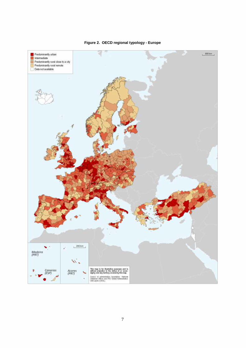
Figure 2. OECD regional typology - Europe

8

Figure 3. OECD Regional typology - Asia

9

Annex: Data inputs for the extension of the OECD regional typology

The accessibility analysis used to build the typology for North America was carried by the OECD

following the methodology proposed by the Directorate General for Regional Policy of the European

10

Commission. The details of this analysis are explained in the following paragraphs. For further information

on the methodology used to build the typology for Europe, please refer to Dijkstra and Poelman (2008)8.

In a first step, based on the share of population living in local rural areas within each region regions

are classified as Predominantly Urban (PU), Intermediate (IN) or Predominantly Rural (PR). An additional

criterion is based on the size of the urban centres contained in the TL3 regions. A region previously

classified as PR (IN), becomes IN (PU) if it contains an urban centre with at least 200 000 (500 000)

inhabitants representing 25% of the regional population. These three categories are known as the OECD

regional typology. In a second step, the OECD regional typology is extended by considering the driving

time of at least 50% of the regional population to the closest populated centre with more than 50 000

inhabitants. This only applies to the IN and PR categories, since by definition the PU regions include

highly populated localities. The result is a typology containing five categories: PU, INC, INR, PRC, and

PRR.

Accessibility Analysis

In order to identify a region as remote it is needed to perform an accessibility analysis. This type of

analysis quantifies the driving time needed for a certain percentage of the population of a region to reach a

populated centre. A region is considered to be remote if at least 50% of its population needs to drive 60

minutes or more to reach a populated centre with more than 50 000 inhabitants. Due to the lack of data,

Hawaii, Alaska and Puerto Rico have been excluded from the accessibility analysis applied to the United

States. The main inputs of the accessibility analysis are:

A map containing the distribution of the population

A road network

A map containing populated centres with at least 50 000 inhabitants

The analysis can be further refined by considering some additional factors that affect the driving

time. This implies the use of a Digital Elevation Model (DEM) and an Urban Areas map.

Distribution of the population

In order to count the number of people living within each TL3 region, it is necessary to know how the

population is distributed along the territory. This information is usually represented by a population density

map in a raster format. Since this type of map was not available for Mexico, it has been created using data

at the locality level from the 2005 census (INEGI). Rural localities were only available as a point feature

class, while urban localities were available as both point and polygon feature class. Hence, the population

density map was built using the rural localities as point feature class and the urban localities as polygon

feature class. To do so, it has been assumed that the rural localities were concentrated and uniformly

distributed around their coordinates. In the case of the United States, the population density map was

created using tract data from the 2000 Census, while for Canada this map was created using block data

from the 2006 census. Population density was then calculated by dividing the population in each tract and

block by its corresponding area.

8. Dijkstra, L. and H. Poelman (2008) “Remote Rural Regions: How the proximity to a city influences the

performances of rural regions” Regional Focus No 1.

http://ec.europa.eu/regional_policy/sources/docgener/focus/2009_01_metropolitan.pdf

11

For the three countries, the population density maps were rasterised. To do so, a first raster map of the

population density was created using a 100 m grid. From this map, a second map was created using a 1 km

grid. This technique reduces the bias caused by the interpolation carried out while assigning a value to the

grid’s cells. As a result, a map of the population density in raster format was obtained, where every cell

corresponds to the population by square kilometre. It is important to bear in mind that this is an

approximation of the real distribution of the population, which is based on the assumptions previously

mentioned.

Road Network

The road network is used to compute the driving time needed to reach urban centres. In the case of

Mexico, the road network provided by INEGI includes many types of roads classified according to their

number of lanes and structures. To simplify the composition of the network, and to deal with the absence

of some interconnections, three main types of roads were chosen: Paved Roads, Non-Paved Roads and

Paths. Despite this dataset being quite complete, there were certain issues that had to be overcome before

using it in the accessibility analysis. In the first place, not all the roads were connected to the network.

Moreover, some pieces of the network were completely isolated. In the second place, since the localities

are represented as a point feature class, they were not connected to the network. To tackle these problems,

the network was cleaned up by removing the isolated segments and a new set of segments to join the

network to the localities was created. In the case of the United States, the road network used for the

analysis comes from the National Transportation Atlas Database. For practical reasons, only national

highways were considered for the analysis. The national highways dataset is composed by 174 540

observations, including interstate, freeways, expressways, and other minor arterials. In the case of Canada,

the road network was obtained from Statistics Canada and it was classified in three types of segments:

highways, roads, and connecting streets.

Populated Centres

For Mexico, populated centres were obtained from the urban localities dataset provided by the INEGI

while for the United States and Canada, these data came from the 2000 Census Gazetteer files and the

North American Atlas, respectively. Once these datasets were filtered, there were 195 populated centres

with at least 50 000 inhabitants in Mexico, 662 in the United States and 52 in Canada.

Additional factors

The driving time to reach a populated centre can be influenced by several factors, in particular, the

driving speeds, the traffic around urban areas and the slope of the roads. To take into account these three

factors, a slope and a density index were computed for the three countries.

The slope index is a proxy for the influence of the terrain. The slope of terrain was calculated using a

digital elevation terrain model. The resulting slope values were reclassified in three intervals: 0% - 5%, 6%

- 11%, and more than 11%. For the first interval, the slope index takes a value equal to 1, while for the

second and third intervals it takes the values of 1.2 and 1.5, respectively.

The density index is a proxy for the congestion around urban areas. This variable assigns a value to

each road segment depending on the type of road it belongs to, and whether the segment is inside of an

urban polygon. In the case of Mexico, for every segment outside an urban polygon the density index takes

a value equal to 1; for segments within an urban polygon, the density index takes a value of 1.5 if the

segment belongs to a paved road, 1.8 if the segment belongs to a non-paved road, and 2 if the road belongs

to a path or if it belongs to one of the segments created to join the localities to the network. In the case of

the United States, two main types of roads have been identified from the national highways dataset:

12

Principal arterials and Minor arterials. Principal arterials include interstate highways, freeways and

expressways, while minor arterials include minor and major collectors as well as local roads. To simplify

the analysis, it was assumed that no traffic is found outside urban areas, while the traffic in urban areas has

a bigger effect on minor arterials than on the principal ones. A weight equal to 1 was given to all road

segments outside an urban area, while Principal and Minor arterials within an urban area respectively

received weights equal to 1.5 and 2. The same type of weighting was used for Canada, where the highways

received a value equal to 1.5, while the roads and connecting streets received a value equal to 2.

Since the speed limits in Mexico often change within the same type of road, choosing a value for

every type of road was not an easy task. Following the recommendations provided by the Ministry of

Communications and Transport to foreigners driving in Mexico, the following values for each type of road

were selected: 100 km/ h for the paved roads, 50 km / h for the non-paved roads and the segments joining

localities to the network, and 30 km / h for the paths. In the US, speed limits are defined by each State,

mainly depending on the land use. However, speed limits may change depending on the time of day and

the type of vehicle. For practical reasons, only day time limits for non-truck vehicles have been used,

taking into account whether a highway segment belongs to an urban or a rural area. In the case of Canada,

the speed limits are defined according to type and location of the road. Indeed, segments of highways

located in rural areas have a maximum speed limit of 100 km/h, while the rest of highway segments are

limited to 80 km/h. Connecting streets have a limit of 50 km/h.

Finally, the road network was intersected with the slope and urban polygons layers to create a road

network where every segment has a specific value assigned for the slope of the terrain and a value to

indicate if the segment belongs to an urban polygon. From this layer, the crossing time of every segment in

the network can be calculated as follows:

Service Areas

To carry on with the accessibility analysis, once the density population map and the road network

were ready, it was necessary to define the service areas surrounding every populated centre with at least

50 000 inhabitants. A service area is a region that encompasses all accessible roads. The size of a service

area depends on the time needed to access a certain point, in this case a populated centre. For instance, a

60-minute service area for a specific locality includes all the roads in the network that can be reached from

that locality within 60 minutes. In Figure 6, the service areas, the localities with more than 50 000

inhabitants and the road network are shown for the east-coast of the U.S. The service areas are represented

by the concentric rings around the localities. These service areas were calculated for different time frames:

30 minutes (yellow), 60 minutes (orange) and 90 minutes (red). In this map, the service areas are

represented by blue concentric polygons surrounding the cities (red points). Light blue polygons represent

a 30 minutes service area, while medium blue and dark blue represent respectively 60 and 90 minutes

service areas.

13

Figure 4. Elements for the accessibility analysis

Using the service areas a region can be classified as remote (or close to a city) by calculating the

percentage of people living within a specific time frame. For the current analysis it has been considered a

60-minute time frame, and a percentage of population of 50%. Hence, if less than 50% of the population

lives within the 60-minute service area, the region was considered to be remote.

The results obtained from this analysis depend on the parameters used to model the accessibility to the

localities, i.e. the crossing time, the size of the localities and the time frame. Initially, two sizes for the

localities had been considered: 50 000 and 100 000 inhabitants. However, based on the definition of a

locality, 50 000 was considered to be a more adequate size. Since cities are composed by localities, using a

bigger size may exclude localities within big cities or metropolitan areas.

Regarding the time frame used for the analysis, the three thresholds shown in Figure 6 were

considered. Since a 30-min drive is common in big countries like Mexico, the United States and Canada, it

was decided to focus on the other two time frames. It can be seen that the classification of regions is

significantly affected by the choice of the time frame. Table 2 shows that for a 60-minutes time frame in

Mexico, 63 regions are classified as remote, while for a 90-min time frame only 38 regions fall in the

category. The decrease in the number of regions is proportional to the decrease in the population for each

class. Using a time frame of 90 minutes reduces the percentage of people living in remote areas by almost

a half. Nevertheless, the distributions of the employment and population growth rate variables, for the 60-

min and 90-min time frames seem to be quite similar. Similarly, in the case of the United States, when

using a 90 minutes the percentage of inhabitants in remote areas is reduced by half, while the number of

regions classified as “Remote” is also significantly reduced, going from 32 to 19 regions. This is also the

case for Canada. For this reason, it was decided to only consider the results of a 60-min time frame.

14

Table 2. Number of regions and percentage of population by typology based on 90 minutes of driving time, Mexico

Close to a City Remote Totals

OECD Typology N. of regions Population N. of regions Population N. of regions Population

IN 33 98% 2 2% 35 100%

Canada PR 99 61% 124 39% 223 100%

PU 30 100% - 0% 30 100%

Total 162 88% 126 12% 288 100%

IN 29 98% 1 2% 30 100%

Mexico PR 107 85% 38 15% 145 100%

PU 34 100% - 0% 34 100%

Total 170 94% 39 6% 209 100%

IN 21 100% 0 0% 21 100%

U.S. PR 112 95% 19 5% 131 100%

PU 25 100% 0 0% 25 100%

Total 158 98% 19 2% 177 100%

15

Figure 5. Service areas for 30-min, 60-min and 90-min time frames, North America

16

NOTES

For Canada the following exceptions have been made when calculating the typology for 2006 Census Divisions:

CA1209 Halifax County (Pr=12, CD=9) has a rurality of 100 in 2001 and 2006 but is classified as "intermediate" (consistent with 1986 and 1996) (the 1996 rurality was 31.0)

CA2410 Rimouski-Neigette (Pr=24, CD=10) has a rurality of 100 in 2006 but is classifed as "intermediate" (consistent with 2001) (the 2001 rurality was 36.2).

CA2425 Lévis (Pr=24, CD=25) has a rurality of 0 in 2006 and is re-classifed as "predominantly urban) (in 2001, the components of the Lévis CD were Desjardins (coded as "intermediate" with a rurality of 21.1 and Les Chutes-de-la-Chaudière (coded as "intermediate" with a rurality of 17.5)

CA2429 Beauce-Sartigan (Pr=24, CD=29) has a rurality of 100 in 2006 byt is classified as "intermediate" to be consistent with 2001 (2001 rurality was 48.0).

CA2436 Shawinigan (Pr=24, CD=36) has a rurality of 100 in 2006 but is coded as "intermediate" to be consistent with 2001 (2001 rurality was 28.7)

CA2439 Arthabaska (Pr=24, CD=39) was "predominantly rural" in 1986 became "intermediate" in 1996 and 2001 (2001 rurality=35.7).

CA2443 Sherbrooke (Pr=24, CD=43) has a rurality of 0 in 2006 and is re-classifed as "predominantly urban" (in 2001, the rurality was 42.3 and it was classified as "intermediate").

CA2445 Memphrémagog (Pr=24, CD=45) was "predominantly rural" in 1986 and 1996 but became intermediate in 2001 (2001 rurality = 46.2).

CA2459 Lajemmerais has a rurality of 16.4 in 2006 but is coded as "predominantly urban" to be consistent with 2001 (2001 rurality was 10.5).

CA2493 Lac-Saint-Jean-Est (Pr=24, CD=93) was "predominantly rural" in 1986 and 1996 but became intermediate in 2001 (2001 rurality = 49.9; 1996 rurality = 50.1)

CA3519 York County (Pr=35, CD=19) was "intermediate" in 1986 and 1996 but became predominantly urban in 2001 (2001 rurality = 13.8; 1996 rurality = 15.7).

CA3524 Halton Regional Municipality (Pr=35, CD=24) was "intermediate" in 1986 and became "predominantly urban" in 1996 and 2001 (2001 rurality=8.4) in 1996

CA3525 Hamilton (formerly, Hamilton-Wentworth) (Pr=35, CD=25) had a rurality=19.5 in 1996 but was classified in 1996 as "predominantly urban" (consistent with 1986) (in 2001, the rurality=0.0 and thus it is "predominantly urban").

CA3529 Brant County (Pr=35, CD=29) has a rurality of 100 in 2001 and 2006 but is classified as "intermediate" (consistent with 1986 and 1996) (the 1996 rurality was 20.3)

CA3534 Elgin County (Pr=35, CD34) has rurality of 42.8 in 2006 and is reclassified as "intermediate" from "predominantly rural" (2001 rurality was 100)

CA3536 Chatham-Kent (Pr=35, CD=36) has a rurality = 100 in 2001 and 2006 but is classified as "intermediate" (consistent with 1986 and 1996) (the 1996 rurality was 43.9).

CA3539 Middlesex County (includes city of London, Ontario) (PR=35, CD=39) has a 2006 rurality = 16.6 and a 2001 rurality=16.5 but is classified as "predominantly urban" (consistent with 1986 and 1996).

CA3553 Greater Sudbury (Pr=35, CD=53) has a rurality of 100 in 2001 and 2006 but is classified as "intermediate" (consistent with 1986 and 1996) (the 1996 rurality was 43.9 percent)

CA4811 Alberta Census Division No. 11 (Pr=48, CD=11)(includes city of Edmonton) has a 2006 rurality =32.1 and a 2001 rurality=31.7 but is classified as "predominantly urban" (consistent with 1986 and 1996).

CA5917 Capital Regional District (Pr=59, CD=17) (includes the city of Victoria, B.C.) has a 2006 rurality = 24.2 and a 2001 rurality=23.0 but is classified as "predominantly urban" (consistent with 1986 and 1996).

CA5921 Nanaimo (Pr=59, CD=21) was "predominantly rural" in 1986 and 1996 but became "predominantly urban" in 2001 (2001 rurality = 11.4).

For Korea the typology has been updated with 2009 data on population and area. The classification has changed for the following regions:

KR013 In 2009 has a rurality of 7.8 and was therefore re-classified from “intermediate” to “Predominantly Urban” KR022 Although the rurality is of 17.8 the region was re-classified, applying the 3

rd criterion, from “intermediate” to

“Predominantly Urban”, as the regions contains an urban centre with a population over a 1 000 000 (Ulsan) KR052 Was re-classified from “Predominantly Rural” to “Intermediate” KR071 Was re-classified from “Intermediate” to “Predominantly Rural”

For France the typology has been revised. The classification has changed for 3 regions (FR511, FR612, FR623), which have been re-classified from “intermediate” to “Predominantly Urban” applying the 3

rd criterion as described in the methodology.